BR

ICS

NS

-01-2B

rookes&

Mislove

(eds.):M

FP

S’01

Prelim

inaryP

roceedings

BRICSBasic Research in Computer Science

Preliminary Proceedings of the 17th Annual Conference on

Mathematical Foundationsof Programming Semantics

MFPS ’01

Aarhus, Denmark, May 24–27, 2001

Stephen BrookesMichael Mislove(editors)

BRICS Notes Series NS-01-2

ISSN 0909-3206 May 2001

Copyright c© 2001, Stephen Brookes & Michael Mislove(editors).BRICS, Department of Computer ScienceUniversity of Aarhus. All rights reserved.

Reproduction of all or part of this workis permitted for educational or research useon condition that this copyright notice isincluded in any copy.

See back inner page for a list of recent BRICS Notes Series publications.Copies may be obtained by contacting:

BRICSDepartment of Computer ScienceUniversity of AarhusNy Munkegade, building 540DK–8000 Aarhus CDenmarkTelephone: +45 8942 3360Telefax: +45 8942 3255Internet: BRICS@brics.dk

BRICS publications are in general accessible through the World WideWeb and anonymous FTP through these URLs:

http://www.brics.dkftp://ftp.brics.dkThis document in subdirectory NS/01/2/

Electronic Notes in Theoretical Computer Science

Volume 45

Mathematical Foundations of Programming SemanticsSeventeenth Annual Conference

Aarhus UniversityAarhus, DenmarkMay 23 – 26, 2001

Guest Editors:S. Brookes M. Mislove

Preliminary ProceedingsFinal Proceedings will be available at

http://www.elsevier.nl/locate/entcs/volume45.html

ii

Table of ContentsForeword . . . . . . . . . . . . . . . . . . . . . . . . . . . . . . . . . . . . . . . . . . . . . . . . . . . . . . . . . . . . . . . . . . . . v

Dedication. . . . . . . . . . . . . . . . . . . . . . . . . . . . . . . . . . . . . . . . . . . . . . . . . . . . . . . . . . . . . . . . . .vii

A Relationship between Equilogical Spaces and Type Two Effectivity. . . . . . . . . . . .1Andrej Bauer

Transfer Principles for Reasoning About Concurrent Programs . . . . . . . . . . . . . . . . 23Stephen Brookes

Time Stamps for Fixed-Point Approximation . . . . . . . . . . . . . . . . . . . . . . . . . . . . . . . . . 43Daniel Damian

A New Approach to Quantitative Domain Theory . . . . . . . . . . . . . . . . . . . . . . . . . . . . .55Lei Fan

A Concurrent Graph Semantics For Mobile Ambients . . . . . . . . . . . . . . . . . . . . . . . . . 67Fabio Gadducci & Ugo Montanari

Regular-Language Semantics for a Call-by-Value Programming Language . . . . . . 85Dan R. Ghica

Typing Correspondence Assertions for Communication Protocols . . . . . . . . . . . . . . .99Andrew D. Gordon & Alan Jeffrey

Pseudo-commutative Monads . . . . . . . . . . . . . . . . . . . . . . . . . . . . . . . . . . . . . . . . . . . . . . 121Martin Hyland & John Power

Stably Compact Spaces and Closed Relations. . . . . . . . . . . . . . . . . . . . . . . . . . . . . . . .133Achim Jung, Mathias Kegelmann & M. Andrew Moshier

A Game Semantics of Idealized CSP . . . . . . . . . . . . . . . . . . . . . . . . . . . . . . . . . . . . . . . . 157J. Laird

Unique Fixed Points in Domain Theory . . . . . . . . . . . . . . . . . . . . . . . . . . . . . . . . . . . . . 177Keye Martin

A Generalisation of Stationary Distributions, and Probabilistic Program Algebra189

A. K. McIver

A Selective CPS Transformation . . . . . . . . . . . . . . . . . . . . . . . . . . . . . . . . . . . . . . . . . . . . 201Lasse R. Nielsen

iii

Semantics for Algebraic Operations . . . . . . . . . . . . . . . . . . . . . . . . . . . . . . . . . . . . . . . . . 223Gordon Plotkin & John Power

An Algebraic Foundation for Graph-based Diagrams in Computing . . . . . . . . . . . . 237John Power & Kostantinos Tourlas

Comparing Control Constructs by Double-barrelled CPS Transforms . . . . . . . . . . 249Hayo Thielecke

Distance and Measurement in Domain Theory . . . . . . . . . . . . . . . . . . . . . . . . . . . . . . .265Pawel Waszkiewicz

iv

ForewordThese are the preliminary proceedings of the Seventeenth Conference on the Math-ematical Foundations of Programming Semantics. The meeting consists of seveninvited talks, given by the following:

Olivier Danvy Joshua Guttman

BRICS MitreNeil Jones Kim Larsen

DIKU AalborgPrakash Panangaden Jan Rutten

McGill CWIGlynn Winskel

Cambridge

There also are three special sessions, whose topics are:

• A session honoring Neil Jones, organized by Olivier Danvy and David

Schmidt. This session begins with an invited address by Professor Danvy,and includes talks by Radhia Cousot, John Hannan, John Hughes,

David Schmidt and Peter Sestoft.

• A session on model checking organized by Gavin Lowe. This commenceswith an invited talk by Kim Larsen, and includes talks by Jose Deshar-

nais, Michael Huth, Henrik Jensen, Marta Kwiatkowska, andGavin Lowe,

• A session on security, organized by Catherine Meadows. This com-mences with an invited talk by Joshua Guttman, and includes talks by An-

drew Gordon and Alan Jeffrey, Gavin Lowe, Thomas Jensen,

Catherine Meadows, and Andre Scedrov.

The remainder of the program is made up of papers selected by the Program Com-mittee from those selected from the submission in response to the Call for Papers.The Program Committee was co-chaired by Stephen Brookes and Michael

Mislove, and included

Lars Birkedal Rance Cleaveland

ITU SUNY, Stony BrookMarcelo Fiore Matthew Hennessy

Cambridge SussexAlan Jeffrey Achim Jung

DePaul BirminghamGavin Lowe Catherine Meadows

Oxford NRLPeter O’Hearn Susan Older

Queen Mary & Westfield Syracuse

v

Dusco Pavlovic Uday Reddy

Kestrel BirminghamGiuseppe Rosolini Davide Sangiorgi

Genoa INRIAAndre Scedrov

Pennsylvania

This year’s meeting is being hosted by Aarhus University, with the local arrangementsbeing carried out by Professors Olivier Danvy and Andrzej Filinski. We are gratefulto these colleagues for their having so efficiently overseen the local arrangements.The Organizers also express their appreciation to Karen Kjær Møller, the chiefsecretary at BRICS for her help with the meeting.

The meeting is being supported by BRICS and by the U. S. Office of NavalResearch. We are grateful to both organizations for making the meeting possible,and we especially thank Dr. R. F. Wachter at ONR who has provided continuedsupport for the MFPS series.

Stephen Brookes Michael MisloveConference Co-chairs

vi

Dedication

The Organizers of the MFPS series dedicate these Proceedings to Neil Jones

for his continuing inspiration to researchers in theoretical computer science. Neilhas been a regular participant in the MFPS series, having been one of the invitedspeakers at the 1987 meeting, and having regularly participated in the series. MFPSappreciates the continued inspiration that his research results have provided, andthat his talks at MFPS have so clearly elucidated.

vii

MFPS 17 Preliminary Version

A Relationship between Equilogical Spacesand Type Two E�ectivity

Andrej Bauer 1

Institut Mittag-Le�er

The Royal Swedish Academy of Sciences

Abstract

In this paper I compare two well studied approaches to topological semantics|

the domain-theoretic approach, exempli�ed by the category of countably based

equilogical spaces, Equ, and Type Two E�ectivity, exempli�ed by the category of

Baire space representations, Rep(B ). These two categories are both locally cartesian

closed extensions of countably based T0-spaces. A natural question to ask is how

they are related.

First, we show that Rep(B ) is equivalent to a full core ective subcategory of Equ,

consisting of the so-called 0-equilogical spaces. This establishes a pair of adjoint

functors between Rep(B ) and Equ. The inclusion Rep(B ) ! Equ and its core ection

have many desirable properties, but they do not preserve exponentials in general.

This means that the cartesian closed structures of Rep(B ) and Equ are essentially

di�erent. However, in a second comparison we show that Rep(B ) and Equ do share a

common cartesian closed subcategory that contains all countably based T0-spaces.

Therefore, the domain-theoretic approach and TTE yield equivalent topological

semantics of computation for all higher-order types over countably based T0-spaces.

We consider several examples involving the natural numbers and the real numbers

to demonstrate how these comparisons make it possible to transfer results from one

setting to another.

1 Introduction

In this paper I compare two approaches to topological semantics|the domain-

theoretic approach, exempli�ed by the category of countably based equilogical

spaces [6,23], Equ, and Type Two E�ectivity (TTE) [27,26,25,14], exempli�ed

by the category of Baire space representations, Rep(B ). These frameworks

have been extensively studied, albeit by two somewhat separate research com-

munities. The present paper relates the two approaches and helps transfer

results between them.

1 E-mail: Andrej.Bauer@andrej.com, URL: http://andrej.com

This is a preliminary version. The �nal version will be published inElectronic Notes in Theoretical Computer Science

URL: www.elsevier.nl/locate/entcs

Bauer

Domain-theoretic models of computation arise from the idea that the re-

sult of a (possibly in�nite) computation is approximated by the �nite stages

of the computation. As the computation progresses, the �nite stages approx-

imate the �nal result ever so better. This leads to a formulation of partially

ordered spaces, called domains, in which every element is the supremum of the

distinguished \�nite" elements that are below it. We recommend [1] and [24]

for an introduction to domain theory.

The TTE framework arises from the study of (possibly in�nite) computa-

tions performed by Turing machines that read in�nite input tapes and write

results on in�nite output tapes. If we view input and output tapes as a se-

quences of natural numbers, then Turing machines correspond to computable

partial operators on the Baire space B = NN . We obtain a purely topological

model of computation by considering all continuous partial operators on B ,

not just the computable ones. We recommend [27] for an introduction to TTE.

The use of equilogical spaces as an exempli�cation of the domain-theoretic

approach to topological semantics needs an explanation. Already in the orig-

inal manuscript [23] Scott showed that equilogical spaces are equivalent to

partial equivalence relations (PERs) on algebraic lattices. He also proved

that the category of algebraic domains is a cartesian closed subcategory of

equilogical spaces, and it is not hard to see that the same holds for continu-

ous lattices. In [6,5] we showed that equilogical spaces are a generalization of

domain theory with totality [9,8,7,20,21]. The crucial observation needed for

those results is that equilogical spaces are equivalent to the category of dense

PERs on algebraic domains (a PER on a domain is said to be dense if its ex-

tension is a dense subset of the domain). The equivalence remains if we take

dense PERs on continuous domains instead. In this sense, it is fair to say that

equilogical spaces generalize several domain-theoretic frameworks and contain

a number of important categories of domains that have been studied, but of

course not all of them. In this paper we focus solely on the countably based

equilogical spaces, and call them simply \equilogical spaces".

As the ambient category of TTE we take the category of Baire space repre-

sentations, Rep(B ), which is de�ned in Section 3. Contemporary formulations

of TTE often use the Cantor space in place of the Baire space, but since we are

not concerned with computational complexity here, it does not matter which

one we use because they yield in equivalent categories. We call Baire space

representations just \representations".

Equilogical spaces and representations both form locally cartesian closed

extensions of the category of countably based T0-spaces, !Top0. Thus they

are both appealing models of computation on topological spaces. This is why

it is important from the programming semantics point of view to understand

precisely how they are related.

The general framework within which we carry out the comparison is realiz-

ability theory, since Equ and PER(B ) are just realizability models; the former

is equivalent to the PER model on the Scott-Plotkin graph model PN , whereas

2

Bauer

the latter is equivalent to the PER model on the Second Kleene Algebra B . We

can then use Longley's theory of applicative morphisms between partial com-

binatory algebras (PCAs) to compare the two PER models [17]. While this

may be the most general and elegant technique that could be used to compare

other semantic frameworks as well, it has a distinctly anti-topological avor.

But we can translate all the results from realizability back into the language

of topology, which is precisely what we do. This immediately gives us the �rst

result: a simple topological description of Rep(B ), without any mention of the

partial combinatory structure of the Second Kleene Algebra.

From the topological description of Rep(B ) so obtained, it is apparent

that Rep(B ) is equivalent to a full subcategory of Equ. This subcategory is

denoted by 0Equ and consists of all the 0-equilogical spaces, which are those

equilogical spaces whose underlying topological spaces are 0-dimensional. The

inclusion I : 0Equ ! Equ has a core ection D : Equ ! 0Equ. These two

functors have many desirable properties, but they do not preserve the function

spaces in general.

We compare Equ and Rep(B ) in another way, by demonstrating that they

share a common cartesian closed subcategory that contains all countably based

T0-spaces. This subcategory was discovered by Menni and Simpson [19,18] as

the category of !-projecting T0-quotients, and by Schr�oder [22] as the category

of sequential T0-spaces with admissible representations. We prove that these

two categories coincide. Therefore, the domain-theoretic approach and TTE

yield equivalent topological semantics of computation for all higher-order types

over countably based T0-spaces.

Finally, we discuss various consequences and the potential for transfer of

results between the two settings, in particular with respect to the natural

numbers, the real numbers, and their higher-order function spaces.

The paper is organized as follows. In Section 1 we review the basic def-

initions and facts about equilogical spaces and !-projecting quotients. In

Section 3 we review Baire space representations and admissible representa-

tions. Sections 4 and 5 contain the two comparisons of Equ and Rep(B ). In

Section 6 we obtain various transfer results between the two settings.

The material presented here is part of my Ph.D. dissertation [4], written

under the supervision of Dana Scott. The omitted proofs can be found in the

dissertation.

I gratefully acknowledge helpful discussions about this topic with Steven

Awodey, Lars Birkedal, Peter Lietz, Alex Simpson, Matthias Schr�oder, and

Dana Scott. Peter and I found the equivalence of 0-equilogical spaces and

Baire space representations together. I could have never proved the coinci-

dence of !-projecting quotients and admissible representations without talking

to Matthias and Alex. I also thank the knowledgeable anonymous referee for

helpful suggestions on how to better present the material.

3

Bauer

2 Equilogical Spaces and !-projecting Quotients

An equilogical space was de�ned by Scott [23,6] to be a T0-space with an

equivalence relation. Here we are only interested in countably based equilog-

ical spaces, which are countably based T0-spaces with equivalence relations.

We denote the category of countably based T0-spaces and continuous maps

by !Top0. We omit the quali�er \countably based" from now on, unless we

are explicitly dealing with spaces that are not countably based.

More precisely, an equilogical space is a pair X = (jXj;�X) where jXj 2

!Top0 and �X is an equivalence relation on the underlying set of jXj. The

associated quotient of an equilogical spaceX is the topological quotient kXk =

jXj=�X. The canonical quotient map jXj ! kXk is denoted by qX . Note

that kXk need not be T0 or countably based. A morphism f : X ! Y between

equilogical spaces X and Y is a continuous map f : kXk ! kY k that is tracked

by some (not necessarily unique) continuous map g : jXj ! jY j, which means

that the following diagram commutes:

jXjg //

qX

��

jY j

qY

��kXk

f// kY k

Any map g that appears in the top row of such a diagram is equivariant, or

extensional, meaning that, for all x; y 2 jXj, x �X y implies gx �Y gy. 2

The category of equilogical spaces and morphisms between them is denoted

by Equ.

An exponential of X and Y is an object E = Y X with a morphism e : E�

X ! Y , called the evaluation map, such that, for all Z and f : Z �X ! Y ,

there exists a unique map ef : Z ! E, called the transpose of f , such that the

following diagram commutes:

E �X

e

""EEEEE

EEEEE

EEEE

Z �X

ef � 1X

OO

f//Y

A weak exponential is de�ned in the same way but without the uniqueness

requirement for ef . A category is said to be cartesian closed when it has the

terminal object, �nite products, and all exponentials. It is locally cartesian

closed when every slice is cartesian closed.

2 We could de�ne morphisms between equilogical spaces to be equivalence classes of equiv-

ariant maps, which is the original de�nition from [23].

4

Bauer

The category Equ is equivalent to the PER model PER(PN) [4, Theo-

rem 4.1.3], which is a regular locally cartesian closed category. This equiva-

lence gives us a description of exponentials in Equ, though a very impractical

one. A somewhat better description can be obtained as follows. Suppose X

and Y are equilogical spaces, and (W; e) is a weak exponential of jXj and jY j

in !Top0. De�ne a relation �E on W by

f �E g () 8 x; y 2 jXj : (x �X y =) e(f; x) �Y e(g; y)) :

Let E = (jEj;�E) be the equilogical space whose underlying space is

jEj =�f 2 W

�� f �E f� W :

It is easy to check that E with the morphism induced by the evaluation map

e : jEj � jXj ! jY j is the exponential of X and Y [4, Proposition 4.1.7]. The

category !Top0 has weak exponentials, thus the following construction shows

that Equ has exponentials. It would be desirable to have a good theory of weak

exponentials of topological spaces, as that would give us better descriptions of

exponentials in Equ. In certain cases (weak) exponentials have good descrip-

tions. For example, if jXj is locally compact and Hausdor�, then the space of

continuous maps W = C(jXj; jY j) with the compact-open topology together

with the usual evaluation map is an exponential of jXj and jY j in !Top0.

Every countably based T0-space X can be viewed as an equilogical space

(X;=X) where =X is equality on X. This de�nes a full and faithful inclusion

functor I : !Top0 ! Equ. The inclusion preserves �nite limits, coproducts,

and all exponentials that already exist in !Top0. Preservation of exponentials

follows directly from the above description of exponentials in Equ.

There is the associated quotient functor Q : Equ ! Top that maps an

equilogical space X to the associated quotient QX = kXk and a morphism

f : X ! Y to the continuous map Qf = f : kXk ! kY k. Here Top is the

category of all topological spaces and continuous maps, because the associated

quotient need not be countably based or T0. Clearly, Q is a faithful functor,

and it is not hard too see that it is not full. Menni and Simpson [19,18]

showed that there is a largest subcategory C of Equ such that Q restricted

to C is full. They worked with equilogical spaces built from all countably

based topological spaces, as opposed to just T0-spaces, but their results hold

when we restrict them to T0-spaces. We are restricting to T0-spaces because

Schr�oder proved his results for T0-spaces. Below we summarize the relevant

�ndings from [19,18].

De�nition 2.1 A subset S � X of a topological space X is sequentially

open when every sequence with limit in S is eventually in S. A topological

space X is a sequential space when every sequentially open set V � X is open

in X. The category of sequential spaces and continuous maps between them

is denoted by Seq.

5

Bauer

Theorem 2.2 Sequential spaces form a cartesian closed category that con-

tains !Top0. The inclusion !Top0 ! Seq preserves �nite limits and all expo-

nentials that already exist in !Top0.

Proof. This is well known and follows from the fact that Seq is a re ective

subcategory of the cartesian-closed category Lim of limit spaces [15], and the

re ection preserves products. 2

De�nition 2.3 Let X 2 !Top0 and q : X ! Y be a continuous map. Then q

is said to be !-projecting when for every Z 2 !Top0 and every continuous

map f : Z ! Y there exists a lifting g : Z ! X such that f = q Æ g.

An equilogical space X is !-projecting when the canonical quotient map

qX : jXj ! kXk is !-projecting. The full subcategory of Equ on the !-

projecting equilogical spaces is denoted by EPQ0. Let PQ0 be the category of

those T0-spaces Y for which there exists an !-projecting map q : X ! Y .

The name PQ0 stands for \!-projecting quotient", and EPQ0 stands for

\equilogical !-projecting quotient".

Theorem 2.4 (Menni & Simpson [19]) The category PQ0 is a cartesian

closed subcategory of Seq, EPQ0 is a cartesian closed subcategory of Equ, and

the categories PQ0 and EPQ0 are equivalent via the restriction of the associated

quotient functor Q : EPQ0 ! PQ0.

Proof. See [19]. In fact, Menni and Simpson prove that PQ0 is the largest

common subcategory C of Equ and Top such that Q restricted to C is full. 2

3 Type Two E�ectivity

In this section we review the basic setup of Type Two E�ectivity. The Baire

space B = NN is the set of all in�nite sequences of natural numbers, equipped

with the product topology. Let N� be the set of all �nite sequences of natural

numbers. The length of a �nite sequence a is denoted by jaj. If a; b 2 N� we

write a v b when a is a pre�x of b. Similarly, we write a v � when a is a pre�x

of an in�nite sequence � 2 B . A countable topological base for B consists of

the basic open sets, for a 2 N� ,

a::B =�a::�

�� � 2 B=�� 2 B

�� a v �:

The expression a::� denotes the concatenation of the �nite sequence a 2 N�

with the in�nite sequence � 2 B . We write n::� instead of [n]::� for n 2 N and

� 2 B . The base�a::B

�� a 2 N�is a clopen countable base for the topology

of B , which means that B is a countably based 0-dimensional T0-space. Recall

that a space is 0-dimensional when its clopen subsets form a base for its

topology. A 0-dimensional T0-space is always Hausdor�.

In order to obtain a simple topological description of Baire space represen-

tations, we need to characterize subspaces of B and those partial continuous

6

Bauer

maps B * B that can be encoded as elements of B . This is accomplished by

the Embedding and Extension Theorems for B , which we prove next.

Theorem 3.1 (Embedding Theorem for B ) A topological space is a 0-

dimensional countably based T0-space if, and only if, it embeds into B .

Proof. Clearly, every subspace of B is a countably based 0-dimensional T0-

space. Suppose X is a countably based 0-dimensional T0-space with a count-

able base�Uk�� k 2 N

of clopen sets. De�ne the map e : X ! B by

ex = �n2N : (if x 2 Un then 1 else 0) :

It is easy to check that e is a topological embedding. 2

For topological spaces X and Y , a partial map f : X * Y is said to be

continuous when the restriction to its domain f : dom(f)! Y is a continuous

(total) map, where dom(f) is equipped with the subspace topology inherited

from X. There is no requirement that dom(f) be an open subset of X. We

consider partial continuous maps B * B and characterize those that can be

encoded as elements of B .

Given a �nite sequence of numbers a = [a0; : : : ; ak�1], let seq a be the

encoding of a as a natural number, for example

seq [a0; : : : ; ak�1] =

k�1Yi=0

pi1+ai ;

where pi is the i-th prime number. For � 2 B let �n = seq [�0; : : : ; �(n� 1)].

For �; � 2 B , de�ne � ? � by

� ? � = n () 9m2N :��(�m) = n + 1 ^ 8 k < m : �(�k) = 0

�:

If there is no m 2 N that satis�es the above condition, then �?� is unde�ned.

Thus, ? is a partial operation B � B * N . It is continuous because the value

of � ? � depends only on �nite pre�xes of � and �. The continuous function

application � j� : B � B ! N * N is de�ned by

(� j �)n = � ? (n::�) :

The Baire space B together with j is a partial combinatory algebra, where � j�

is considered to be unde�ned when � j � is not a total function, see [13] for

details. Every � 2 B represents a partial function �� : B * B de�ned by

��� = � j � :

We say that a partial map f : B * B is realized when there exists � 2 B such

that f = ��. Such an � is called a realizer for f . Because j is a continuous

operation, a realized map is always continuous, although not every partial

7

Bauer

continuous map is realized. Recall that a GÆ-set is a set that is equal to a

countable intersection of open sets.

Proposition 3.2 If U � B is a GÆ-set then the function u : B * B de�ned

by

u� =

(�n :N : 1 � 2 U ;

unde�ned otherwise

is realized.

Proof. The set U is a countable intersection of countable unions of basic

open sets, U =Ti2N

Sj2N ai;j::B . De�ne a sequence � 2 B for all i; j 2 N by

�(seq (i::ai;j)) = 2, and set �n = 0 for all other arguments n. Clearly, if ���

is total then its value is �n: 1, so we only need to verify that dom(��) = U .

If � 2 dom(��) then � ? (i::�) is de�ned for every i 2 N , therefore there

exists ci 2 N such that �(seq (i::[�0; : : : ; �(ci)])) = 2, which implies that

� 2 ai;ci. Hence � 2Ti2N ai;ci::B � U . Conversely, if � 2 U then for

every i 2 N there exists some ci 2 N such that � 2 ai;ci. For every i 2 N ,

�(seq (i::[�0; : : : ; �(ci)])) = 2, therefore (���)i = � ? (i::�) = 1. Hence � 2

dom(��). 2

Corollary 3.3 Suppose � 2 B and U � B is a GÆ-set. Then there exists

� 2 B such that �� = �� for all 2 dom(��) \ U and dom(��) = U \

dom(��).

Proof. By Proposition 3.2 there exists � 2 B such that for all � 2 B

��� =

(�n :N : 1 � 2 U ;

unde�ned otherwise :

It suÆces to show that the function f : B * B de�ned by

(f�)n = ((���)n) � ((���)n)

is realized. This is so because coordinate-wise multiplication of sequences is

realized, and so are pairing and composition. 2

Theorem 3.4 (Extension Theorem for B ) (a) Every partial continuous

map B * B can be extended to a realized one. (b) The realized partial maps

B * B are precisely those continuous partial maps whose domains are GÆ-sets.

Proof. (a) Suppose f : B * B is a partial continuous map. Consider the set

A � N�� N

2 de�ned by

A =�ha; i; ji 2 N

�� N

2��

a::B \ dom(f) 6= ; and 8�2 (a::B \ dom(f)) : ((f�)i = j):

8

Bauer

If ha; i; ji 2 A, ha0; i; j 0i 2 A and a v a0 then j = j 0 because there exists

� 2 a0::B \ dom(f) � a::B \ dom(f) such that j = (f�)i = j 0. We de�ne

a sequence � 2 B as follows. For every ha; i; ji 2 A let �(seq (i::a)) = j + 1,

and for all other arguments let �n = 0. Suppose that �(seq (i::a)) = j + 1

for some i; j 2 N and a 2 N� . Then for every pre�x a0 v a, �(seq (i::a0)) = 0

or �(seq (i::a0)) = j + 1. Thus, if ha; i; ji 2 A and a v � then � ? (i::�) = j.

We show that (���)i = (f�)i for all � 2 dom(f) and all i 2 N . Because f is

continuous, for all � 2 dom(f) and i 2 N there exists ha; i; ji 2 A such that

a v � and (f�)i = j. Now we get (���)i = (� j �)i = � ? (i::�) = j = (f�)i.

(b) First we show that �� is a continuous map whose domain is a GÆ-set.

It is continuous because the value of (���)n depends only on n and �nite

pre�xes of � and �. The domain of �� is the GÆ-set

dom(��) =�� 2 B

�� 8n2N : ((� j �)n de�ned)

=\n2N

�� 2 B

�� (� j �)n de�ned=\n2N

[m2N

�� 2 B

�� � ? (n::�) = m:

Each of the sets�� 2 B

�� � ? (n::�) = mis open because ? and :: are contin-

uous operations. Now let f : B * B be a partial continuous function whose

domain is a GÆ-set. By part (a) of this theorem there exists � 2 B such that

f� = ��� for all � 2 dom(f). By Corollary 3.3 there exists 2 B such that

dom(� ) = dom(f) and � � = ��� for every � 2 dom(f). 2

A Baire space representation, or simply a representation, is a partial sur-

jection ÆS : B * S, where S is a set. A representation ÆS : B * S of a set S

induces a quotient topology on S, de�ned by

U � S open () Æ�1S (U) open in dom(ÆS) :

We denote by kSk the topological space S with the quotient topology induced

by ÆS. A realized map f : (S; ÆS) ! (T; ÆT ) is a function f : S ! T such

that there exists a partial continuous map g : B * B which tracks f , meaning

that dom(f) � dom(g) and that, for every � 2 dom(f), f(ÆS�) = ÆT (g�). A

realized map f is always continuous as map f : kSk ! kTk. The category of

Baire space representations and realized maps is denoted by Rep(B ).

The category Rep(B ) is equivalent to the PER model PER(B ) where B is

equipped with the structure of the Second Kleene Algebra. The objects of

PER(B ) are partial equivalence relations on B . If A is a PER on B we denote

it by A when we think of it as an object and by =A when we think of it as a

binary relation. For A;B 2 PER(B ), we say that � 2 B realizes a morphism

[�] : A! B when, for all �; 2 B , if � =A , then � j � and � j are de�ned,

and � j� =B � j . Here � and �0 realize the same morphism, [�] = [�0], when,

for all �; 2 B , � =A implies � j� =B �0j . The equivalence of Rep(B ) and

9

Bauer

PER(B ) assigns to each representation ÆS : B * S the PER =S de�ned by

� =S � () ÆS(�) = ÆS(�) :

If f : (S; ÆS)! (T; ÆT ) is a realized map in Rep(B ), tracked by g : B * B , then

by Extension Theorem 3.4 there exists � 2 B such that �� is a continuous

extension of g. Under the equivalence Rep(B ) ' PER(B ), the morphism f

corresponds to the morphism [��]. The most relevant consequence of this

equivalence is that Rep(B ) is a regular locally cartesian closed category, since

every PER model on a PCA is such a category [4]. For example, the expo-

nential BA of PERs A;B 2 PER(B ) is de�ned by

� =BA �0() 8 �; 2 B : (� =A =) (� j �) # =B (�0 j ) #) :

Unfortunately, this description of exponentials in not very helpful in particular

cases, and it completely obscures the topological properties of exponentials.

In many important cases better descriptions are available, cf. Theorem 4.5.

In TTE we are typically interested in representations of topological spaces,

rather than arbitrary sets. For this reason it is important to represent a

topological space X with a representation (X; ÆX) which has a reasonable

relation to the topology of X. An obvious requirement is that the original

topology of X should coincide with the quotient topology of kXk. However,

as is well known by the school of TTE, this requirement is too weak because it

allows ill-behaved representations. A desirable condition on representations of

topological spaces is that all continuous maps between them be realized. Thus,

we are led to further restricting the allowable representations of topological

spaces as follows.

De�nition 3.5 An admissible representation of a topological space X is a

partial continuous quotient map Æ : B * X such that every partial continuous

map f : B * X can be factored through Æ. This means that there exists

g : B * B such that f� = Æ(g�) for all � 2 dom(f).

The main e�ect of this de�nition is that if ÆX : B * X and ÆY : B * Y are

admissible representations, then every continuous map f : X ! Y is realized,

and conversely, every realizer that respects ÆX and ÆY induces a continuous

map X ! Y .

The requirement that and admissible representation Æ : B * X be a quo-

tient map implies that X is a sequential space, since it is a quotient of the

sequential space dom(Æ). It is easy to show that any two admissible repre-

sentations are isomorphic in Rep(B ). An obvious question to ask is which

sequential spaces have admissible representations.

De�nition 3.6 Let AdmSeq be the full subcategory of Seq on those sequential

T0-spaces that have admissible representations. 3

3 It is believed that the T0 requirement is inessential for the results proved here, but that

10

Bauer

Schr�oder [22] has characterized AdmSeq as follows.

De�nition 3.7 [Schr�oder [22]] A pseudobase for a space X is a family B of

subsets of X such that whenever hxnin2N !O(X) x1 and x1 2 U 2 O(X)

then there exists B 2 B such that x1 2 B � U and hxnin2N is eventually

in B.

Theorem 3.8 (Schr�oder [22]) A sequential T0-space has an admissible rep-

resentation if, and only if, it has a countable pseudobase.

From Schr�oder's proof of Theorem 3.8 we get a speci�c admissible rep-

resentation Æ for a T0-space X with a countable pseudobase�Bk

�� k 2 N,

de�ned by

Æ(�) = x ()

8 k 2N : (x 2 B�k) ^ 8U 2O(X) : (x 2 U =) 9 k 2N : B�k � U) :

The above formula says that � is a Æ-representation of x when � enumerates

(indices of) a sequence of pseudobasic open neighborhoods of x that get arbi-

trarily small. In case X is a T0-space with a countable base�Uk�� k 2 N

, we

may use an equivalent but simpler admissible representation Æ0, de�ned by

Æ0(�) = x ()�U�k

�� k 2 N=�Un�� n 2 N ^ x 2 Un

:

The above formula says that � is a Æ0-representation of x when it enumerates

the basic open neighborhoods of x.

If X 2 AdmSeq then its admissible representation is determined up to iso-

morphism in Rep(B ). Therefore, AdmSeq is equivalent to the full subcategory

of Rep(B ) on the admissible representations, so that AdmSeq can be thought of

as a subcategory of Rep(B ). The following result by Schr�oder [22] tells us that

the inclusion of AdmSeq into Rep(B ) preserves the cartesian closed structure.

Theorem 3.9 (Schr�oder [22]) Let (X; ÆX) and (Y; ÆY ) be admissible repre-

sentations for sequential T0-spaces X and Y . Then the product (X; ÆX) �

(Y; ÆY ) formed in Rep(B ) is an admissible representation of the product X�Y

formed in Seq, and similarly the exponential (Y; ÆY )(X;ÆX ) formed in Rep(B ) is

an admissible representation for the exponential Y X formed in Seq.

4 Rep(B ) as a subcategory of Equ

In this section we describe Rep(B ) as a full subcategory of equilogical spaces.

We then study the properties of the inclusion Rep(B ) ! Equ.

De�nition 4.1 A 0-equilogical space is an equilogical space whose underlying

topological space is 0-dimensional. The category 0Equ is the full subcategory

of Equ on 0-equilogical spaces.

has not been checked yet.

11

Bauer

Thus 0Equ is formed just like Equ, where we use 0Dim instead of !Top0.

Theorem 4.2 The categories 0Equ, Rep(B ), and PER(B ) are equivalent.

Proof. We show that 0Equ and PER(B ) are equivalent, since we already know

that PER(B ) and Rep(B ) are equivalent. By Embedding Theorem 3.1 for B , a

countably based T0-space is 0-dimensional if, and only if, it embeds in B . Thus

every 0-equilogical space is isomorphic to one whose underlying topological

space is a subspace of B . This make it clear that equivalence relations on

0-dimensional countably based T0-spaces correspond to partial equivalence

relations on B . Morphisms work out, too, since by the Extension Theorem

for B 3.4 every partial continuous map on B can be extended to a realized

one. 2

The inclusion functor I : 0Equ! Equ has a right adjoint D : Equ! 0Equ,

which is de�ned as follows. For every countably based T0-space X there exists

an admissible representation ÆX : B * X. The subspace X0 = dom(Æ) � B

is a countably based 0-dimensional Hausdor� space. Now if X = (jXj;�X)

is an equilogical space, let DX = (X0;�DX) where a �DX b if, and only if,

ÆXa �X ÆXb. If f : X ! Y is a morphism in Equ, tracked by g : jXj ! jY j,

then Df is the morphism tracked by a continuous map h : X0 ! Y0 that tracks

g : X ! Y , as shown in the following commutative diagram:

X0h //

ÆX

��

Y0

ÆY

��X g

//Y

Such a map h exists because ÆX and ÆY were chosen to be admissible repre-

sentations. The main properties of the adjoints I a D are summarized in the

following theorem.

Theorem 4.3

(i) Functors I and D are a section and a retraction, i.e., D Æ I is naturally

equivalent to 10Equ.

(ii) I is full and faithful and preserves countable colimits and limits (which

are precisely all the limits and colimits that exist in Equ).

(iii) D is faithful and preserves countable limits and colimits (which are pre-

cisely all the limits and colimits that exist in 0Equ).

(iv) D is not full, but its restriction to EPQ0 is full.

Proof. (i) This follows by a general category-theoretic argument from the

fact that I is full and faithful, cf. the dual of [11, Proposition 3.4.1].

(ii) It is obvious that I is full and faithful since it is just the inclusion

functor of a full subcategory. It preserves colimits because it is a left adjoint,

12

Bauer

and it preserves limits because the inclusion 0Dim! !Top0 does.

(iii) It is obvious that D is faithful, and it preserves limits because it is

a right adjoint. That D preserves �nite colimits can be veri�ed explicitly,

and it also follows from [17, Proposition 2.5.11]. That D preserves countable

coproducts holds because a countable coproduct of admissible representations

is again an admissible representation.

(iv) If D were full then by [11, Proposition 3.4.3] it would follow that

the counit of the adjunction � : I ÆD ! 1Equ is a natural isomorphism, which

obviously is not the case. For example, �R is not a natural isomorphism, where

R are the real numbers equipped with the Euclidean topology, because every

morphism R ! I(DR) is constant, as it must be tracked by a continuous map

from R into the 0-dimensional Hausdor� space jI(DR)j. However, when D is

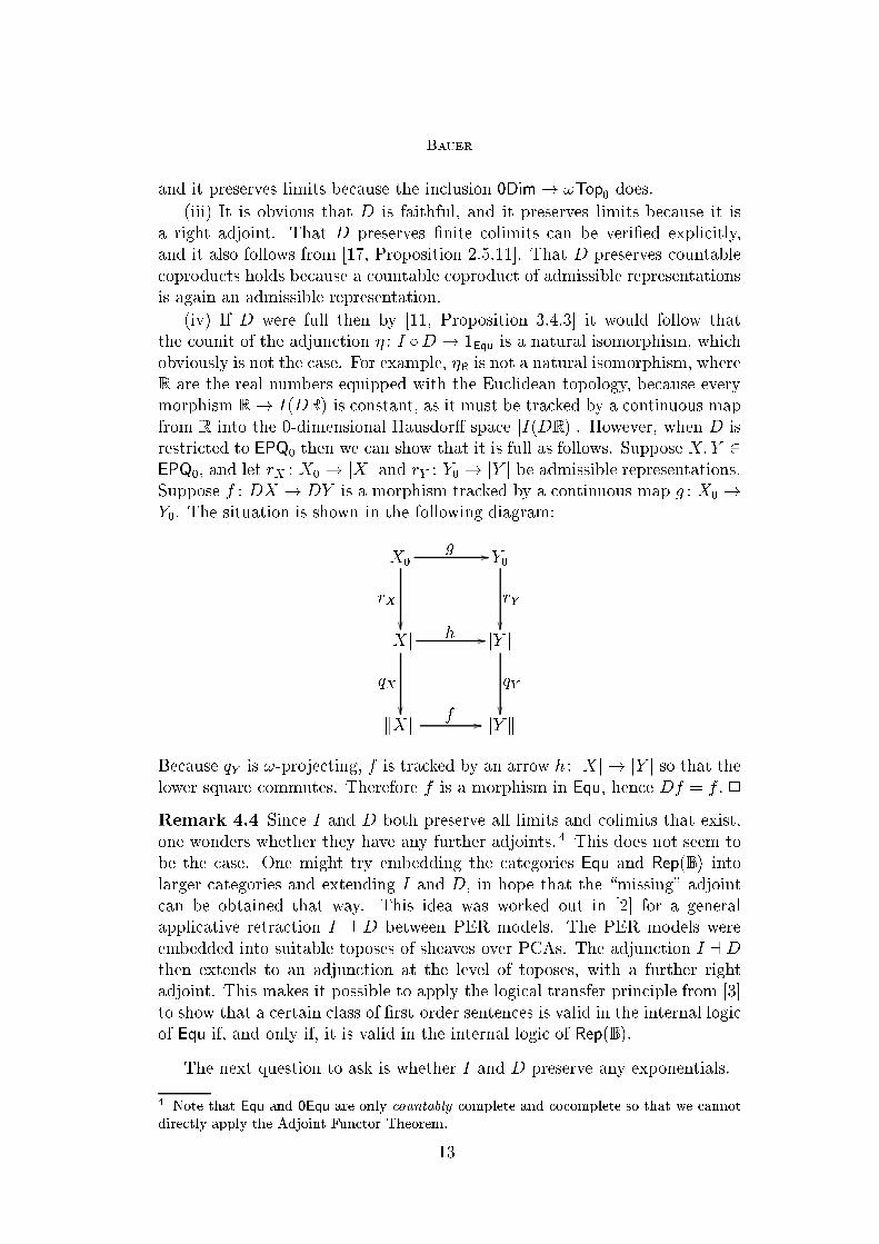
restricted to EPQ0 then we can show that it is full as follows. Suppose X; Y 2

EPQ0, and let rX : X0 ! jXj and rY : Y0 ! jY j be admissible representations.

Suppose f : DX ! DY is a morphism tracked by a continuous map g : X0 !

Y0. The situation is shown in the following diagram:

X0

g //

rX

��

Y0

rY

��jXj h //

qX

��

jY j

qY

��kXk

f // kY k

Because qY is !-projecting, f is tracked by an arrow h : jXj ! jY j so that the

lower square commutes. Therefore f is a morphism in Equ, hence Df = f . 2

Remark 4.4 Since I and D both preserve all limits and colimits that exist,

one wonders whether they have any further adjoints. 4 This does not seem to

be the case. One might try embedding the categories Equ and Rep(B ) into

larger categories and extending I and D, in hope that the \missing" adjoint

can be obtained that way. This idea was worked out in [2] for a general

applicative retraction I a D between PER models. The PER models were

embedded into suitable toposes of sheaves over PCAs. The adjunction I a D

then extends to an adjunction at the level of toposes, with a further right

adjoint. This makes it possible to apply the logical transfer principle from [3]

to show that a certain class of �rst-order sentences is valid in the internal logic

of Equ if, and only if, it is valid in the internal logic of Rep(B ).

The next question to ask is whether I and D preserve any exponentials.

4 Note that Equ and 0Equ are only countably complete and cocomplete so that we cannot

directly apply the Adjoint Functor Theorem.

13

Bauer

Theorem 4.5

(i) Functor D restricted to EPQ0 preserves exponentials.

(ii) If X; Y 2 0Equ and there exists in !Top0 a 0-dimensional weak exponen-

tial of jXj and jY j, then I preserves the exponential Y X .

(iii) Functor I preserves the natural numbers object N, the exponentials NN

and 2N, and the object Rc of Cauchy reals.

(iv) Functor I does not preserve exponentials in general. In particular, it does

not preserve NNN

.

Proof. (i) This follows from results obtained in Section 5, and so we postpone

the proof until then. It can be found on page 16.

(ii) If W 2 0Dim is a weak exponential of X and Y in !Top0, then it is

also a weak exponential of X and Y in 0Dim. Therefore, the construction of

Y X from W in Equ, as described in Section 2 coincides with the one in 0Equ.

(iii) The Baire space NN and the Cantor space 2N both satisfy the condition

from (ii). The real numbers object Rc is a regular quotient of N � 2N [4,

Proposition 5.5.3], and the left adjoint I preserves it because it preserves N ,

2N, products, and coequalizers.

(iv) Let X = NNN

in 0Equ, and let Y = NNN

in Equ. The space jXj is

a Hausdor� space. The space jY j is the subspace of the total elements of

the Scott domain DY = [N?!! N? ]. The equivalence relation on jY j is the

consistency relation of DY restricted to jY j. Suppose f : jY j ! jXj repre-

sented an isomorphism, and let g : jXj ! jY j represent its inverse. Because f

is monotone in the specialization order and jXj has a trivial specialization

order, a �Y b implies fx = fy. Therefore, g Æ f : jY j ! jY j is an equivariant

retraction. By [4, Proposition 4.1.8], Y is a topological object. By [4, Corol-

lary 4.1.9], this would mean that the topological quotient kY k is countably

based, but it is not, as is well known. Another way to see that Y cannot

be topological is to observe that Y is an exponential of the Baire space, but

the Baire space is not exponentiable in !Top0, and in particular NNN

is not a

topological object in Equ. 2

Remark 4.6 In [2] we used a logical transfer principle between Equ and

Rep(B ) to prove that I does not preserve RcRc either.

As already mentioned in the introduction, we could obtain the results of

this section by applying Longley's theory of applicative adjunctions between

applicative morphisms of partial combinatory algebras [17]. Lietz [16] used

this approach to compare the realizability toposes RT(PN) and RT(B ).

5 A Common Subcategory of Equ and Rep(B )

In Sections 2 and 3 we saw that sequential spaces contain cartesian closed

subcategories PQ0 and AdmSeq which are also cartesian closed subcategories

14

Bauer

of Equ and Rep(B ), respectively. In this section we prove that PQ0 and AdmSeq

are the same category.

Lemma 5.1 Suppose B =�Bi

�� i 2 Nis a countable pseudobase for a count-

ably based T0-space Y . Let X be a �rst-countable space and f : X ! Y a con-

tinuous map. For every x 2 X and every neighborhood V of fx there exists a

neighborhood U of x and i 2 N such that fx 2 f(U) � Bi � V .

Proof. Note that the elements of the pseudobase do not have to be open

sets, so this is not just a trivial consequence of continuity of f . We prove the

lemma by contradiction. Suppose there were x 2 X and a neighborhood V

of fx such that for every neighborhood U of x and for every i 2 N , if Bi � V

then f�(U) 6� Bi. Let U0 � U1 � � � � be a descending countable neighborhood

system for x. Let p : N ! N be a surjective map that attains each value

in�nitely often, that is for all k; j 2 N there exists i � k such that pi = j. For

every i 2 N , if Bpi � V then f�(Ui) 6� Bpi. Therefore, for every i 2 N there

exists xi 2 Ui such that if Bpi � V then fxi 62 Bpi. The sequence hxnin2Nconverges to x, hence hfxnin2N converges to fx. Because B is a pseudobase

there exists j 2 N such that Bj � V and hfxnin2N is eventually in Bj, say

from the k-th term onwards. There exists i � k such that pi = j. Now we get

fxi 2 Bpi � V , which is a contradiction. 2

Theorem 5.2 PQ0 and AdmSeq are the same category.

Proof. It was independently observed by Schr�oder that PQ0 is a full subcat-

egory of AdmSeq, which is the easier of the two inclusions. The proof goes

as follows. Suppose q : X ! Y is an !-projecting quotient map. We need

to show that Y is a sequential space with an admissible representation. It

is sequential because it is a quotient of a sequential space. There exists an

admissible representation ÆX : B * X. Let ÆY = q Æ ÆX . Suppose f : B * Y

is a continuous partial map. Because q is !-projecting f lifts though X, and

because ÆX is an admissible representation, it further lifts through B .

It remains to prove the converse, namely that if a sequential T0-space X

has an admissible representation then there exists an !-projecting quotient

q : Y ! X. Since X has an admissible representation it has a countable

pseudobase B =�Bi

�� i 2 N, by Theorem 3.8. The powerset PN ordered by

inclusion is an algebraic lattice. We equip it with the Scott topology, which

is generated by the subbasic open sets "n =�a 2 PN

�� n 2 a, n 2 N . Let

q : PN * X be a partial map de�ned by

qa = x ()

(8n2 a : x 2 Bn) ^ 8U 2O(X) : (x 2 U =) 9n2 a : Bn � U) :

The map q is well de�ned because qa = x and qa = y implies that x and y

share the same neighborhoods, so they are the same point of the T0-space X.

Furthermore, q is surjective because B is a pseudobase. To see that p is

15

Bauer

continuous, suppose pa = x and x 2 U 2 O(X). There exists n 2 N such that

x 2 Bn � U . If n 2 b 2 dom(p) then pb 2 Bn � U . Therefore, a 2 "n and

p�("n) � Bn � U , which means that p is continuous. Let Y = dom(p).

Let us show that q : Y ! X is !-projecting. Suppose f : Z ! X is a

continuous map and Z 2 !Top0. De�ne a map g : Z ! PN by

gz =�n 2 N

�� 9U 2O(Z) : (z 2 U ^ f�(U) � Bn):

The map g is continuous almost by de�nition. Indeed, if gz 2 "n then there

exists a neighborhood U of z such that f�(U) � Bn, but then g�(U) 2 "n. To

�nish the proof we need to show that fz = p(gz) for all z 2 Z. If n 2 gz then

fz 2 Bn because there exists U 2 O(Z) such that z 2 U and f�(U) � Bn.

If fz 2 V 2 O(X) then by Lemma 5.1 there exists U 2 O(Z) and n 2 N

such that z 2 U and f�(U) � Bn � U . Hence, n 2 gz. This proves that

fz = p(gz). 2

Remark 5.3 Matthias Schr�oder has showed recently that if a sequential T0-

space X arises as a topological quotient of a subspace of B , then X has an

admissible representation. This result implies Theorem 5.2, and also gives a

very nice characterization of EPQ0: it is precisely the category of all T0-spaces

that are topological quotients of countably based T0-spaces.

The relationships between the categories are summarized by the following

diagram:

Seq Equ ' PER(PN)

Da

��

!Top0 //PQ0 = AdmSeq

44iiiiiiiiiiiiiiiiiiiii

**UUUUUUUUUUUUUUUUUUUUU

OO

0Equ ' Rep(B ) ' PER(B )

I

OO

(1)

The unlabeled arrows are full and faithful inclusions, preserve countable limits,

and countable coproducts. The inclusion !Top0 ! PQ0 preserves all exponen-

tials that happen to exist in !Top0, and the other three unlabeled inclusions

preserve cartesian closed structure. The right-hand triangle involving the two

inclusions and the core ection D commutes up to natural isomorphism (and

the one involving the inclusion I does not).

We still owe the proof of Theorem 4.5(i), namely, thatD restricted to EPQ0

preserves exponentials. But this is now obvious, since the right-hand triangle

involving D commutes.

6 Transfer Results between Equ and Rep(B )

The correspondence (1) explains why domain-theoretic computational models

agree so well with computational models studied by TTE|as long as we

16

Bauer

only build spaces by taking products, coproducts, exponentials, and regular

subspaces, starting from countably based T0-spaces, we remain in PQ0, the

common cartesian closed core of equilogical spaces and TTE.

As a �rst example of a transfer result, we translate a characterization of

Kleene-Kreisel countable functionals [12] from Equ to Rep(B ). In [6] we proved

that the iterated exponentials N , NN , NNN

, : : : of the natural numbers object N

in Equ are precisely the Kleene-Kreisel countable functionals. Because N is

the natural numbers object in Rep(B ) as well, and it belongs to PQ0, the same

hierarchy appears in Rep(B ).

Proposition 6.1 In Rep(B ), the hierarchy of exponentials N, NN , NNN

, : : : ,

built from the natural numbers object N , corresponds to the Kleene-Kreisel

countable functionals.

As a second example, we consider transfer between the internal logics

of Equ and Rep(B ). Because Equ and Rep(B ) are equivalent to realizability

models PER(PN) and PER(B ), respectively, they admit a realizability inter-

pretation of �rst-order intuitionistic logic. This has been worked out in detail

in [4]. It is often advantageous to work in the internal logic, because it lets us

argue abstractly and conceptually about objects and morphisms. We never

have to mention explicitly the realizers of morphisms or the underlying topo-

logical spaces, which makes arguments more perspicuous. Every map that can

be de�ned in the internal logic is automatically realized (and computable, if

we work with the computable versions of the realizability models).

Suppose we want to use internal logic to construct a particular map f : X !

Y where X; Y 2 PQ0. For example, we might want to de�ne the de�nite in-

tegration operator I : R[0;1]! R,

If =

Z 1

0

f(x) dx :

It may happen that X and Y are much more amenable to the internal logic

of Rep(B ) than to the internal logic of Equ, or vice versa. In such a case we

can pick whichever internal logic is better and work in it, because if a map

f : X ! Y is de�nable in one internal logic, then it exists as a morphism in

both Equ and Rep(B ).

Let us see how this applies in the case of de�nite integration. The real num-

bers R are much better behaved in Rep(B ) than in Equ, because R can be char-

acterized in the internal logic of Rep(B ) as the Cauchy complete Archimedean

�eld, which gives us all the properties of R we could wish for. On the other

hand, in the internal logic of Equ, R does not seem to be characterizable at

all, and it does not even satisfy the Archimedean axiom

8 x2R : 9n2 N : x < n ;

because in Equ there is no continuous choice map c : R ! N that would

17

Bauer

satisfy x < cx for all x 2 R. 5 This makes it impractical to argue about R

in the internal logic of Equ. The situation with the space R[0;1] of continuous

real function on the unit interval is similar|it is much better behaved in

the internal logic of Rep(B ) than in the internal logic of Equ. In particular,

in Rep(B ) the statement \every map f : [0; 1] ! R is uniformly continuous"

is valid, whereas it is not valid in the internal logic of Equ. This makes it

clear that the internal logic of Rep(B ) is the better choice. Indeed, in the

internal logic of Rep(B ) de�nite integral may be de�ned in the usual way as

a limit of Riemann sums. The convergence of Riemann sums can then be

proved constructively because Rep(B ) \believes" that all maps from [0; 1] to

R are uniformly continuous. Once we have constructed the de�nite integral

operator I : R[0;1]! R in Rep(B ), we can transfer it to Equ via PQ0.

7 Conclusion

Let me conclude by commenting on the following comparison of domain theory

and TTE from Weihrauch's recently published book on computable analysis

[27, Section 9.8, p. 267]:

\The domain approach developed so far is consistent with TTE. Roughly speak-

ing, a domain (for the real numbers) contains approximate objects as well as

precise objects which are treated in separate sets in TTE. A computable do-

main function must map also all approximate objects reasonably. In many cases,

constructing a domain which corresponds to given representation still is a diÆ-

cult task. Concepts for handling multi-valued functions and for computational

complexity have not yet been developed for the domain approach. The elegant

handling of higher type functions in domain theory can be simulated in TTE by

means of function space representations [Æ ! Æ0] (De�nition 3.3.13). To date,

there seems to be no convincing reason to learn domain theory as a prerequisite

for computable analysis."

The present paper provides a precise mathematical comparison of TTE

and the domain approach, as exempli�ed by equilogical spaces. The corre-

spondence (1) gives us a clear picture about the relationships between the

domain approach and TTE. Overall, it supports the claim that these two ap-

proaches are consistent, at least as far as computability on PQ0 is concerned.

Indeed, domains are built from the approximate as well as the precise

objects, and I join Weihrauch in pointing out that it is a good idea to distin-

guish the precise objects from the approximate ones. In domain theory this is

most easily done by taking seriously domains with totality, or more generally

PERs on domains, which leads to the notion of equilogical spaces and domain

representations, which were studied by Blanck [10].

5 The Archimedean axiom is valid in Rep(B ) because there is a continuous choice map

jDRj ! N such that [a] < ca for all a 2 jDRj, where [a] the real number represented by the

realizer a. The point is that ca may depend on the realizer a.

18

Bauer

I hope that the adjoint functors I and D between Equ and Rep(B ) will ease

the task of constructing a domain which corresponds to a given representation.

Power-domains are the domain-theoretic models of non-deterministic com-

putation, and I believe they could be used to model multi-valued functions.

In this paper we did not consider the computational complexity or even

computability in Equ and Rep(B ). In [4] the inclusion Rep(B ) ! Equ and its

core ection are constructed for the computable versions of equilogical spaces

and TTE, from which we may conclude that computability in domain theory

is essentially the same as in TTE.

By Theorem 4.5, the higher type function spaces in equilogical spaces do

not generally agree with the corresponding function space representations in

TTE. However, the two approaches to higher types do agree on an impor-

tant class of spaces, namely the category PQ0, which contains all countably

based T0-spaces, therefore also all countably based continuous and algebraic

domains. Higher types seem not to catch a lot of interest in the TTE com-

munity. This may be because the descriptions of higher types in terms of

representations can get quite unwieldy and are hard to work with. The the-

ory of cartesian closed categories and the internal logic of Rep(B ) ought to

be helpful here, as they allows us to talk about the higher types abstractly,

without having to refer to their representations all the time. After all, higher

types cannot be ignored in computable analysis: real numbers are a quotient

of type 1, integration and di�erentiation operators have type 2, solving a dif-

ferential equation is a type 3 process, and still higher types are reached when

we study spaces of distributions and operators on Hilbert spaces.

Finally, is there a convincing reason to learn domain theory as a prereq-

uisite for computable analysis? By Theorem 4.2, Rep(B ) is a full subcategory

of Equ. This may suggest the view that the domain approach is more general

than TTE. At any rate, they are not competing approaches. They �t with

each other very well, and each has its advantages: domain theory handles

higher types more elegantly and is more general than TTE, whereas TTE

provides a more convenient internal logic and handles questions about com-

putational complexity better. So why not learn both, and a bit of category

theory, realizability, and constructive logic on top?

References

[1] Amadio, R. and P.-L. Curien, \Domains and Lambda-Calculi," Cambridge

Tracts in Theoretical Computer Science 46, Cambridge University Press, 1998.

[2] Awodey, S. and A. Bauer, Sheaf toposes for realizability (2000), available at

http://andrej.com/papers.

[3] Awodey, S., L. Birkedal and D. Scott, Local realizability toposes and a modal

logic for computability, in: L. Birkedal, J. van Oosten, G. Rosolini and D. Scott,

19

Bauer

editors, Tutorial Workshop on Realizability Semantics, FLoC'99, Trento, Italy,

1999, Electronic Notes in Theoretical Computer Science 23 (1999).

[4] Bauer, A., \The Realizability Approach to Computable Analysis and Topology,"

Ph.D. thesis, Carnegie Mellon University (2000), available as CMU technical

report CMU-CS-00-164 and at http://andrej.com/thesis.

[5] Bauer, A. and L. Birkedal, Continuous functionals of dependent types and

equilogical spaces, in: Computer Science Logic 2000, 2000, available at http:

//andrej.com/papers.

[6] Bauer, A., L. Birkedal and D. Scott, Equilogical spaces, Preprint submitted to

Elsevier (1998).

[7] Berger, U., Total sets and objects in domain theory, Annals of Pure and

Applied Logic 60 (1993), pp. 91{117, available at http://www.mathematik.

uni-muenchen.de/~berger/articles/apal/diss.dvi.Z.

[8] Berger, U., \Continuous Functionals of Dependent and Transitive Types,"

Habilitationsschrift, Ludwig-Maximilians-Universit�at M�unchen (1997).

[9] Berger, U., E�ectivity and density in domains: A survey, , 23 (2000).

[10] Blanck, J., \Computability on Topological Spaces by E�ective Domain

Representations," Ph.D. thesis, Department of Mathematics, Uppsala

University (1997).

[11] Borceux, F., \Handbook of Categorical Algebra I. Basic Category Theory,"

Encyclopedia of Mathematics and Its Applications 51, Cambridge University

Press, 1994.

[12] Kleene, S., Countable functionals, in: Constructivity in Mathematics, 1959, pp.

81{100.

[13] Kleene, S. and R. Vesley, \The Foundations of Intuitionistic Mathematics,

especially in relation to recursive functions," North-Holland Publishing

Company, 1965.

[14] Kreitz, C. and K. Weihrauch, Theory of representations, Theoretical Computer

Science 38 (1985), pp. 35{53.

[15] Kuratowski, C., \Topologie," Warszawa, 1952.

[16] Lietz, P., Comparing realizability over P! and K2 (1999), available at http:

//www.mathematik.tu-darmstadt.de/~lietz/comp.ps.gz.

[17] Longley, J., \Realizability Toposes and Language Semantics," Ph.D. thesis,

University of Edinburgh (1994).

[18] Menni, M. and A. Simpson, The largest topological subcategory of countably-

based equilogical spaces, in: Preliminary Proceedings of MFPS XV, 1999,

available at http://www.dcs.ed.ac.uk/home/als/Research/.

20

Bauer

[19] Menni, M. and A. Simpson, Topological and limit-space subcategories of

countably-based equilogical spaces (2000), submitted to Math. Struct. in Comp.

Science.

[20] Normann, D., Categories of domains with totality (1998), available at http:

//www.math.uio.no/~dnormann/.

[21] Normann, D., The continuous functionals of �nite types over the reals, Preprint

Series 19, University of Oslo (1998).

[22] Schr�oder, M., Admissible representations of limit spaces, in: J. Blanck,

V. Brattka, P. Hertling and K. Weihrauch, editors, Computability and

Complexity in Analysis, Informatik Berichte 272 (2000), pp. 369{388, cCA2000

Workshop, Swansea, Wales, September 17{19, 2000.

[23] Scott, D., A new category? (1996), unpublishedManuscript. Available at http:

//www.cs.cmu.edu/Groups/LTC/.

[24] Stoltenberg-Hansen, V., I. Lindstr�om and E. Gri�or, \Mathematical Theory of

Domains," Number 22 in Cambridge Tracts in Computer Science, Cambridge

University Press, 1994.

[25] Weihrauch, K., Type 2 recursion theory, Theoretical Computer Science 38

(1985), pp. 17{33.

[26] Weihrauch, K., \Computability," EATCS Monographs on Theoretical

Computer Science 9, Springer, Berlin, 1987.

[27] Weihrauch, K., \Computable Analysis," Springer-Verlag, 2000.

21

22

MFPS 17 Preliminary Version

Transfer Principles for Reasoning About

Concurrent Programs

Stephen Brookes

Department of Computer Science

Carnegie Mellon University

Pittsburgh, USA

Abstract

In previous work we have developed a transition trace semantic framework, suitable

for shared-memory parallel programs and asynchronously communicating processes,

and abstract enough to support compositional reasoning about safety and liveness

properties. We now use this framework to formalize and generalize some techniques

used in the literature to facilitate such reasoning. We identify a sequential-to-

parallel transfer theorem which, when applicable, allows us to replace a piece of a

parallel program with another code fragment which is sequentially equivalent, with

the guarantee that the safety and liveness properties of the overall program are

una�ected. Two code fragments are said to be sequentially equivalent if they satisfy

the same partial and total correctness properties. We also specify both coarse-

grained and �ne-grained version of trace semantics, assuming di�erent degrees of

atomicity, and we provide a coarse-to-�ne-grained transfer theorem which, when

applicable, allows replacement of a code fragment by another fragment which is

coarsely equivalent, with the guarantee that the safety and liveness properties of

the overall program are una�ected even if we assume �ne-grained atomicity. Both

of these results permit the use of a simpler, more abstract semantics, together with

a notion of semantic equivalence which is easier to establish, to facilitate reasoning

about the behavior of a parallel system which would normally require the use of a

more sophisticated semantic model.

1 Introduction

It is well known that syntax-directed reasoning about behavioral properties

of parallel programs tends to be complicated by the combinatorial explosion

1 This research is sponsored in part by the National Science Foundation (NSF) under GrantNo. CCR-9988551. The views and conclusions contained in this document are those of theauthor, and should not be interpreted as representing the oÆcial policies, either expressedor implied, of the NSF or the U.S. government.2 Email: brookes@cs.cmu.edu

This is a preliminary version. The �nal version will be published inElectronic Notes in Theoretical Computer Science

URL: www.elsevier.nl/locate/entcs

Brookes

inherent in keeping track of dynamic interactions between code fragments.

Simple proof methodologies based on state-transformation semantics, such as

Hoare-style logic, do not adapt easily to the parallel setting, because they

abstract away from interaction and only retain information about the initial

and �nal states observed in a computation. A more sophisticated semantic

model is required, in which an accurate account can be given of interaction.

Trace semantics provides a mathematical framework in which such rea-

soning may be carried out [2,3,4,5]. The trace set of a program describes all

possible patterns of interaction between the program and its \environment",

assuming fair execution [9]. One can de�ne both a coarse-grained trace se-

mantics, in which assignment and boolean expression evaluation are assumed

to be executed atomically, and a �ne-grained trace semantics, in which reads

and writes (to shared variables) are assumed to be atomic. Trace semantics

can be de�ned denotationally, and is fully abstract with respect to a notion of

program behavior which subsumes partial correctness, total correctness, safety

properties, and liveness properties [2].

To some extent program proofs may be facilitated by a number of laws of

program equivalence, validated by trace semantics, which allow us to deduce

properties of a program by analyzing instead a semantically equivalent pro-

gram with simpler structure. The use of a succinct and compact notation for

trace sets (based on extended regular expressions) can also help streamline

program analysis. Yet the problem remains that in general the trace set of a

program can be diÆcult to manipulate and hard to use to establish correct-

ness properties. Trace sets tend to be rather complex mathematical objects,

since a trace set describes all possible interactions between the program and

any potential environment. For the same reason, both the coarse- and the

�ne-grained trace semantics induce a rather discriminating notion of semantic

equivalence, and few laws of equivalence familiar from the sequential setting

also hold in all parallel contexts. It can therefore be diÆcult to establish

trace equivalence of programs merely by direct manipulation of the seman-

tic de�nitions, or by using trace-theoretic laws of program equivalence in a

syntax-directed manner.

In practice, parallel systems ought to be designed carefully to ensure that

the interactions between component processes are highly disciplined and con-

strained. Moreover, when analyzing the properties of code to be run in tightly

controlled contexts, we ought to be able to work within a simpler semantic

model (or, at least, within a reduced subset of the trace semantics) whose

simplicity re ects this discipline. Correspondingly, whenever we know that a

program fragment will be used in a limited form of context, we would like to

be able to employ forms of reasoning which take advantage of the limitations.

For example, we might know that a piece of code is going to be used

\sequentially" inside a parallel program (in a manner to be made precise

soon) and want to use Hoare-style reasoning about this code in establishing

safety and liveness properties of the whole program. It is not generally safe

24

Brookes

to do so, since laws of program equivalence that hold in the sequential setting

cease to be valid in parallel languages because of the potential for interference

between concurrently executing code. Yet local variables can only be accessed

by processes occurring within a syntactically prescribed scope, and cannot be

changed by any other processes running concurrently, so we ought to be able

to take advantage of this non-interference property to simplify reasoning about

code which only a�ects local variables. In particular, when local variables are

only ever used sequentially, in a context whose syntactic structure guarantees

that no more than one process ever gains concurrent access, we should be

able to employ Hoare-style reasoning familiar from the sequential setting. We

would like to know the extent to which this idea can be made precise, and

when this technique is applicable.

In a similar vein, it is usually regarded as realistic to assume �ne-grained

atomicity when trying to reason about program behavior, but more convenient

to make the less realistic but simplifying assumption of coarse granularity,

since this assumption may help to reduce the combinatorial explosion. We

would like to be able to identify conditions under which it is safe to do so.

A number of ad hoc techniques have been proposed along these lines in the

literature, usually without detailed consideration of semantic foundations [1].

Their common aim is to facilitate concurrent program analysis by allowing

replacement of a code fragment by another piece of code with \simpler" be-

havioral properties that permit an easier correctness proof.

In this paper we use the trace-theoretic framework to formalize and gener-

alize some of these techniques. By paying careful attention to the underlying

semantic framework we are able to recast these techniques in a more precise

manner and we can be more explicit about the (syntactic and semantic) as-

sumptions upon which their validity rests. Since these techniques allow us

to deduce program equivalence properties based on one semantic model by

means of reasoning carried out on top of a di�erent semantic model, we refer

to our results as transfer principles. We provide transfer principles speci�cally

designed to address the two example scenarios used for motivation above: a

sequential-to-parallel transfer principle allowing use of Hoare-style reasoning,

and a coarse-to-�ne transfer principle governing the use of coarse semantics

in �ne-grained proofs of correctness.

Our work can be seen as further progress towards a theory of context-

sensitive development of parallel programs, building on earlier work of Cli�

Jones [8] and spurred on by the recent Ph. D. thesis of J�uergen Dingel [7]. We

focus our attention initially on some methodological ideas presented in Greg

Andrews's book on concurrent programming [1]. Later we intend to explore

more fully the potential of our framework as a basis for further generalization

and to extend our results to cover some of the contextual re�nement ideas

introduced by Dingel.

In this preliminary version of the paper we omit explicit details of the

underlying trace semantics, which the reader can �nd in [2], and we omit

25

Brookes

most of the proofs, which require detailed use of the semantic de�nitions.

2 Syntax

2.1 The programming language

Our parallel programming language is described by the following abstract

grammar for commands c, in which b ranges over boolean-valued expressions,

e over integer-valued expressions, x over identi�ers, a over atomic commands

(�nite sequences of assignments), and d over declarations. The syntax for

expressions is conventional and is assumed to include the usual primitives for

arithmetic and boolean operations.

c ::= skip j x:=e j c1; c2 j if b then c1 else c2 j

while b do c j local d in c j

await b then a j c1kc2

d ::= x = e j d1; d2

a ::= skip j x:=e j a1; a2

A command of form await b then a is a conditional atomic action, and causes

the execution of a without interruption when executed in a state satisfying the

test expression b; when executed in a state in which b is false the command

idles. .

A sequential program is just a command containing no await and no par-

allel composition.

Assume given the standard de�nitions of free(e) and free(b), the set of

identi�ers occurring free in an expression. We will use the standard de�nitions

of free(c) and free(d) for the sets of identi�ers occurring free in a command

or a declaration, and dec(d), the set of identi�ers declared by d.

2.2 Parallel, atomic, and sequential contexts

A context is a command which may contain a syntactic \hole" (denoted [�])

suitable for insertion of another command. Formally, the set of (parallel)

contexts, ranged over by C, is described by the following abstract grammar,

in which c1; c2 again range over commands:

C ::= [�] j skip j x:=e j C; c2 j c1;C j

if b then C else c2 j if b then c1 else C j

while b do C j local d in C j

await b then a j

Ckc2 j c1kC

26

Brookes

Note that our abstract grammar for contexts only allows at most one hole to

appear in any particular context. It would be straightforward to adopt a more

general notion of multi-holed context, but the technical details would become

more involved and in any case there is no signi�cant loss of generality.

We also introduce the notion of an atomic context, i.e. a parallel context

whose hole occurs inside the body of an await command. We will use A to

range over atomic contexts.

A sequential context is a limited form of context in which the hole never

appears in parallel. We can characterize the set of sequential contexts, ranged

over by S, as follows:

S ::= [�] j skip j x:=e j S; c2 j c1;S j

if b then S else c2 j if b then c1 else S j

while b do S j local d in S j

await b then a j c1kc2

The important point in this de�nition is that c1kS is not a sequential context

even when S is sequential, but we do allow \harmless" uses of parallelism

inside sequential contexts, as for example in (c1kc2); [�]. The key feature is

that sequentiality of S ensures that when we �ll the hole with a command we

have the guarantee that the command will not be executed concurrently with

any of the rest of the code in S.

We write C[c] for the command obtained by inserting c into the hole of C.

We use similar notation A[a] for the result of inserting an atomic command

a into an atomic context A, and S[c] for the result of inserting a (parallel)

command c into a sequential context S.

It is easy to de�ne the set free(C) of identi�ers occurring free in a context

C, as usual by structural induction. Similarly we let free(S) and free(A)

be the sets of identi�ers occurring free in sequential context S and in atomic

context A.

Contexts may also have a binding e�ect, since the hole in a context may

occur inside the scope of one or more (nested) declarations, and free occur-

rences of identi�ers in a code fragment may become bound after insertion into

the hole. For example, the context

local y = 0 in ([�]ky:=z + 1)

binds y, but not z. On the other hand, the context

(local y = 0 in c1)k([�]; c2)

does not bind any identi�er, since the hole does not occur inside a subcommand

of local form.

To be precise about this possibility we make the following de�nition. We

also make use of analogous notions for sequential contexts and for atomic

27

Brookes

contexts, which may be de�ned in the obvious analogous way. Although we

will not prove this here, it follows from the de�nition that (except for the case

of a degenerate context with no hole) for all contexts C and commands c,

free(C[c]) = free(C) [ (free(c)� bound(C)).

De�nition 2.1 For a context C, let bound(C) be the set of identi�ers for

which there is a binding declaration enclosing the hole in C, de�ned as follows:

bound([�]) = ;

bound(x:=e) = ;

bound(C; c2) = bound(c1;C) = bound(C)

bound(if b then C else c2) = bound(if b then c1 else C) = bound(C)

bound(while b do C) = bound(C)

bound(await b then a) = ;

bound(Ckc2) = bound(c1kC) = bound(C)

bound(local d in C) = bound(C) [ dec(d)

3 Semantics

3.1 Operational semantics

We assume conventional coarse-grained and �ne-grained operational semantics

for expressions and commands [2]. In both cases command con�gurations have

the form hc; si, where c is a command and s is a state. A state s determines a

(�nite, partial) function from identi�ers to variables, and a \store" mapping

variables to their \current" integer values. A transition of form

hc; si ! hc0; s0i

represents the e�ect of c performing an atomic step enabled in state s, resulting

in a change of state to s0, with c0 remaining to be executed. A terminal

con�guration, in which all parallel component commands have terminated, is

represented by a (�nal) state s. In a �ne-grained semantics reads and writes to

variables are atomic, but assignments and boolean condition evaluations need

not be. In a coarse-grained semantics, assignments and boolean expressions

are atomic.

A computation of a command c is a �nite sequence of transitions, ending

in a terminal con�guration, or an in�nite sequence of transitions that is fair

to all parallel component commands of c. (We may also refer to a �ne-grained

computation or a coarse-grained computation, when we need to be precise

about which granularity assumption is relevant.) We write hc; si !�hc0; s0i

to indicate a �nite, possibly empty, sequence of transitions; and hc; si !! to

indicate the existence of a (weakly) fair in�nite computation starting from a

28

Brookes

given con�guration. An interactive computation is a �nite or in�nite sequence

of transitions in which the state may be changed between steps, representing

the e�ect of other commands executing in parallel. There is an analogous

notion of fairness for interactive computations. A computation is just an

interference-free interactive computation, that is, an interactive computation

in which no external changes occur.

3.2 State-transformation semantics and sequential equivalence

De�nition 3.1 The standard state-transformation semantics for programs,

denoted M, is characterized operationally by:

M(c) = f(s; s0) j hc; si !� s0g [ f(s;?) j hc; si !!g:

De�nition 3.2 Two programs c1 and c2 are sequentially equivalent, written

c1 �M c2, if and only if M(c1) =M(c2).

As is well known, sequential equivalence is a congruence with respect to

the sequential subset of our programming language. In fact, for all parallel

programs c1 and c2, and all sequential contexts S,

c1 �M c2 , S[c1] �M S[c2]:

However, the analogous property fails to hold for parallel contexts, because,

for example, we have:

x:=x+ 2 �M x:=x + 1; x:=x + 1

but

x:=x+ 2ky:=x 6�M (x:=x+ 1; x:=x+ 1)ky:=x:

3.3 Trace semantics

A transition trace of a program c is a �nite or in�nite sequence of steps,

each step being a pair of states that represents the e�ect of a �nite se-

quence of atomic actions performed by the program. A particular trace

(s0; s00)(s1; s

01) : : : (sn; s

0n) : : : of c represents a possible fair interactive compu-

tation of c in which the inter-step state changes (from s00to s1, and so on) are

assumed to be caused by processes executing concurrently to c. Traces are

\complete", representing an entire interactive computation, rather than \par-

tial" or \incomplete". A trace is interference-free if the state never changes

between successive steps along the trace, i.e. in the notation used above when

we have s0i= si+1 for all i. An interference-free trace represents a sequence of

snapshots of the state taken during an interference-free fair computation.

Again we obtain both a coarse-grained notion of trace, based on the coarse

interpretation of atomicity and the coarse-grained operational semantics, and

a �ne-grained notion of trace, based on the �ne interpretation of atomicity and

the �ne-grained operational semantics. Both coarse- and �ne-grained trace

29

Brookes

semantics interpret conditional atomic actions await b then a as atomic.

The coarse-grained trace semantics, which we will denote Tcoarse , also assumes

that assignments and boolean expression evaluations are atomic. The �ne-

grained semantics, denoted T�ne , assumes only that reads and writes to simple

variables are atomic. In the rest of this paper, when stating a result which

holds for both �ne- and coarse-grained semantics, we may use T to stand for

either version of the trace semantic function.

Trace semantics can be de�ned compositionally, and we note in particular

that the traces of c1kc2 are obtained by forming fair merges of a trace of c1with a trace of c2, and the traces of c1; c2 are obtained by concatenating a trace

of c1 with a trace of c2, closing up under stuttering and mumbling as required.

The traces of local x = e in c do not change the value of (the \global" version

of) x, and are obtained by projection from traces of c in which the value of

(the \local" version of) x is never altered between steps.

A parallel program denotes a trace set closed under two natural conditions

termed stuttering and mumbling, which correspond to our use of a step to rep-

resent �nite sequences of actions: idle or stuttering steps of form (s; s) may be

inserted into traces, and whenever two adjacent steps (s; s0)(s0; s00) share the

same intermediate state they can be combined to produce a mumbled trace

which instead contains the step (s; s00). The closure properties ensure that

trace semantics is fully abstract with respect to a notion of behavior which

assumes that we can observe the state during execution. As a result trace

semantics supports compositional reasoning about safety and liveness proper-

ties. Safety properties typically assert that no \bad" state ever occurs when a

process is executed, without interference, from an initial state satisfying some

pre-condition. A liveness property typically asserts that some \good" state

eventually occurs. When two processes have the same trace sets it follows

that they satisfy identical sets of safety and liveness properties, in all parallel

contexts.

3.4 Fine- and coarse-grained semantic equivalences

When using coarse-grained semantics one can safely use algebraic laws of

arithmetic to simplify reasoning about program behavior. For instance, in

coarse-grained trace semantics the assignments x:=x + x and x:=2 � x are

equivalent. This feature can be used to considerable advantage in program

analysis. However, coarse granularity is in general an unrealistic assumption

since implementations of parallel programming languages do not generally

guarantee that assignments are indeed executed indivisibly.

The �ne-grained trace semantics is closer in practice to conventional imple-

mentations, but less convenient in program analysis. When using �ne-grained

semantics one cannot assume with impunity that algebraic laws of expression

equivalence remain valid. For instance, the assignments x:=x+x and x:=2�x

are not equivalent in �ne-grained trace semantics; this re ects the fact that

30

Brookes

the former reads x twice, so that if x is changed during execution (say from

0 to 1), the value assigned may be 0; 1 or 2, whereas the latter assignment

(under the same circumstances) would assign either 0 or 2.

It should be clear from the above discussion, even without seeing all of

the semantic de�nitions, that despite the connotations suggested by our use

of \�ne" vs. \coarse", these two trace semantic variants induce incomparable

notions of semantic equivalence. Let us write

c1 �coarse c2 , Tcoarse(c1) = Tcoarse(c2)

c1 ��ne c2 , T�ne(c1) = T�ne(c2)

For instance, we have already seen a pair of programs which are equivalent in

coarse-grained semantics but not in �ne-grained:

x:=x+ x �coarse x:=2� x; x:=x + x 6��ne x:=2� x;

so that c1 �coarse c2 does not always imply c1 ��ne c2.

The converse implication also fails, as shown by the programs x:=x + x

and

local y = 0; z = 0 in (y:=x; z:=x; x:=y + z)

These are equivalent in �ne-grained but not in coarse-grained semantics.

Despite the incomparability of �ne-grained equivalence and coarse-grained

equivalence, for any particular program c the coarse-grained trace set will be

a subset of its �ne-grained traces:

Tcoarse(c) � T�ne(c);

so that it is reasonable to refer to the coarse-grained semantics as \simpler".

We also remark that the state-transformation semantics of a parallel pro-

gram is determined by its trace semantics, in fact by its interference-free traces,

since (s; s0) 2 M(c) if and only if (s; s0) 2 T�ne(c), and (s;?) 2 M(c) if and

only if there is an in�nite interference-free trace in T�ne(c) beginning from

state s. (Here we adopt the usual pun of viewing (s; s0) simultaneously as a

pair belonging to M(c) and as a trace of length 1 belonging to T (c). Such a

trace is trivially interference-free.)

Each trace equivalence is a congruence for the entire parallel language, so

that for all contexts C and parallel commands c1 and c2 we have:

c1 �coarse c2 , C[c1] �coarse C[c2]

c1 ��ne c2 , C[c1] ��ne C[c2]

Moreover, c1 ��ne c2 implies c1 �M c2, but the converse implication is not

generally valid.

4 Reads and writes of a command

To prepare the ground for our transfer principles, we �rst need to de�ne for

each parallel program c the multiset reads(c) of identi�er occurrences which

31

Brookes

appear free in non-atomic sub-expressions of c. It is vital here, as suggested

by the terminology, to keep track of how many references the program makes,

to each identi�er. We need only be concerned with non-atomic subphrases,

since these are the only ones whose execution may be a�ected by concurrent

activity.

We also need to refer to the analogous notions for expressions and for

declarations; since we have not provided a full grammar for expressions we

will give details only for a few key cases, which suÆce for understanding all

of the examples which follow and which convey the general ideas.

For precise mathematical purposes, we may think of a multiset as a set

of identi�ers equipped with a non-negative multiplicity count. In the empty

multiset every identi�er has multiplicity 0. When M1 and M2 are multisets,

we let M1 [+ M2 be the multiset union in which multiplicities are added, and

M1 [max M2 be the multiset union in which multiplicities are combined using

max. That is, an identi�er x which occurs n1 times in M1 and n2 times in M2

will occur n1 + n2 times in M1 [+ M2 and max(n1; n2) times in M1 [max M2.

We write fjxjg for the singleton multiset containing a single occurrence of

x. We also write fj jg for the empty multiset. The cardinality of a multiset M

is denoted jM j.

Each version of union is symmetric and associative:

M1 [+ M2 = M2 [+ M1

M1 [+ (M2 [+ M3) = (M1 [+ M2) [+ M3

M1 [max M2 =M2 [max M1

M1 [max (M2 [max M3) = (M1 [max M2) [max M3

In addition, [max is idempotent:

M [max M =M

Obviously [+ is not idempotent.

The empty multiset is a unit for both forms of union, since

M [+ fj jg = M [max fj jg = M:

Given a multiset M and a set X of identi�ers, we de�ne M �X to be the

multiset obtained fromM by removing all occurrences of identi�ers in X, and

we let M \ X be the multiset consisting of those members of M which are

also in X, with the same multiplicities as they have in M .

We are now ready to de�ne the read multiset of an expression. Again we

include only a few representative cases. Note that we will use the additive

form of multiset union for an expression of form e1 + e2 (and also, in general,

for expressions built with binary operators), because we want to count the

number of times an identi�er needs to be read during the evaluation of an

expression.

32

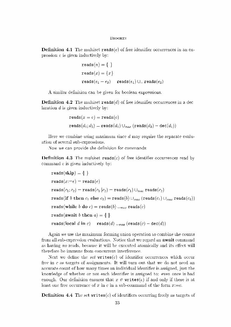
Brookes

De�nition 4.1 The multiset reads(e) of free identi�er occurrences in an ex-

pression e is given inductively by:

reads(n) = fj jg

reads(x) = fjxjg

reads(e1 + e2) = reads(e1) [+ reads(e2)

A similar de�nition can be given for boolean expressions.

De�nition 4.2 The multiset reads(d) of free identi�er occurrences in a dec-

laration d is given inductively by:

reads(x = e) = reads(e)

reads(d1; d2) = reads(d1) [max (reads(d2)� dec(d1))

Here we combine using maximum since d may require the separate evalu-

ation of several sub-expressions.

Now we can provide the de�nition for commands:

De�nition 4.3 The multiset reads(c) of free identi�er occurrences read by

command c is given inductively by:

reads(skip) = fj jg

reads(x:=e) = reads(e)

reads(c1; c2) = reads(c1kc2) = reads(c1) [max reads(c2)

reads(if b then c1 else c2) = reads(b) [max (reads(c1) [max reads(c2))

reads(while b do c) = reads(b) [max reads(c)

reads(await b then a) = fj jg

reads(local d in c) = reads(d) [max (reads(c)� dec(d))

Again we use the maximum-forming union operation to combine the counts

from all sub-expression evaluations. Notice that we regard an await command

as having no reads, because it will be executed atomically and its e�ect will

therefore be immune from concurrent interference.

Next we de�ne the set writes(c) of identi�er occurrences which occur

free in c as targets of assignments. It will turn out that we do not need an

accurate count of how many times an individual identi�er is assigned, just the

knowledge of whether or not each identi�er is assigned to: even once is bad

enough. Our de�nition ensures that x 2 writes(c) if and only if there is at

least one free occurrence of x in c in a sub-command of the form x:=e.

De�nition 4.4 The set writes(c) of identi�ers occurring freely as targets of

33

Brookes

assignment in c is given by:

writes(skip) = ;

writes(x:=e) = fxg

writes(c1; c2) = writes(c1kc2) = writes(c1) [ writes(c2)

writes(if b then c1 else c2) = writes(c1) [ writes(c2)

writes(while b do c) = writes(c)

writes(await b then a) = writes(a)

writes(local d in c) = writes(c)� dec(d)

5 Concurrent reads and writes of a context

Next we de�ne, for each parallel context C, the pair crw(C) = (R;W ), where

R is the set of identi�ers which occur free in evaluation contexts concurrent

to a hole of C, and W is the set of identi�ers occurring free in assigning con-

texts concurrent to a hole. As usual the de�nition is inductive. It suÆces to

work with sets here rather than multisets, since what matters for our present

purposes is whether or not the context may change an identi�er's value concur-

rently while whatever command occupies the hole is running, not how many

times the context may do this; even once is bad enough.

De�nition 5.1 The concurrent-reads-and-writes of a context C are given by:

crw([�]) = crw(skip) = crw(x:=e) = (;; ;)

crw(C; c2) = crw(c1;C) = crw(C)

crw(if b then c1 else C) = crw(if b then C else c2) = crw(C)

crw(while b do C) = crw(C)

crw(await b then a) = (;; ;)

crw(local d in C) = crw(C)

crw(ckC) = crw(Ckc) = (R [ reads(c);W [ writes(c));

where (R;W ) = crw(C)

Note that the clause for local d in C may include in the concurrent reads

and writes some of the identi�ers declared by d; when code is inserted into

the context occurrences of these identi�ers become bound, but we still need

to know if and how the code uses these identi�ers concurrently.

34

Brookes

6 Transfer principles

We now state some fundamental properties of trace semantics, which formalize

the sense in which the behavior of a parallel program depends only on the

values of its free identi�ers. We say that two states s and s0 agree on a set X

of identi�ers if they map each identi�er in this set to (variables which have) the

same integer value. These properties are analogues in the parallel setting of

\Agreement" properties familiar from the sequential setting. Their proofs are

straightforward structural inductions based on the trace semantic de�nitions.

Theorem 6.1 Let � be a trace of c and (s; s0) be a step of �. Then s agrees

with s0 on all identi�ers not in writes(c). 2

Theorem 6.2 Let (s0; s00)(s1; s

01) : : : (sn; s

0n) : : : be a trace of c. Then for every

sequence of states t0; t1; : : : ; tn; : : : such that for all i � 0, ti agrees with si on

X � reads(c), there is a trace

(t0; t0

0)(t1; t

0

1) : : : (tn; t

0

n) : : :

of c such that for all i � 0, t0iagrees with ti on X [ writes(c). 2

Having set up the relevant background de�nitions and this key agreement

lemma we can now present the transfer principles to which we have been

leading.

6.1 A transfer principle for atomic contexts

The �rst one is almost too obvious to include: it suÆces to use sequential

reasoning about any code used in a syntactically atomic context. This holds

in both coarse- and �ne-grained semantics, so we will use �T to stand for

either form of trace equivalence.

Theorem 6.3 If A is an atomic context and a1 �M a2, then A[a1] �T A[a2].

Proof. The traces of await b then a depend only on the \atomic" traces of

a, i.e. on the traces of a which represent uninterrupted complete executions;

and (s; s0) is an atomic trace of a i� (s; s0) 2 M(a). 2

6.2 A sequential transfer principle

The next transfer principle identi�es conditions under which sequential equiva-

lence of code fragments can safely be relied upon to establish trace equivalence

of parallel programs.

Theorem 6.4 If free(c1) [ free(c2) � bound(C), and (R;W ) = crw(C),

and

jreads(ci) \W j+ jwrites(ci) \ Rj = 0; i = 1; 2

then

c1 �M c2 ) C[c1] �T C[c2]: 2

35

Brookes

It is worth noting that the provisos built into this theorem are essential. If

we omit the local declaration around the context the result becomes invalid,

since the assumption that c1 and c2 are sequentially equivalent is not strong

enough to imply that c1 and c2 are trace equivalent. And if we try to use

the code fragments in a context with which it interacts non-trivially again the

result fails: when c1 and c2 are sequentially equivalent it does not follow that

local d in (ckc1) and local d in (ckc2) are trace equivalent for all c, even if

d declares all of the free identi�ers of c1 and c2. A speci�c counterexample is

obtained by considering the commands

c1 : x:=x + 1; x:=x + 1

c2 : x:=x

We have reads(ci) = fjxjg, writes(ci) = fxg. Let C be the context

local x = 0 in (([�]kx:=2); y:=x):

Then bound(C) = fxg and crw(C) = (;; fxg). Using the notation of the

theorem, we have

jreads(ci) \W j = 1; jwrites(ci) \Rj = 0

so that the assumption is violated. And it is easy to see that c1 �M c2, but

C[c1] �T y:=0 or y:=1 or y:=2

C[c2] �T y:=0 or y:=2

so that C[c1] 6�T C[c2].3

Another example shows that the other half of the assumption cannot be

relaxed. Consider

c1 : x:=1; while true do skip

c2 : x:=2; while true do skip

Let C be the context

local x = 0 in ([�]ky:=x):

Then bound(C) = fxg, free(ci) = writes(ci) = fxg, and reads(ci) = fj jg.

Moreover c1 �M c2, since M(ci) = f(s;?) j s 2 Sg (i = 1; 2). We have

jreads(ci) \W j = 0; jwrites(ci) \Rj = 1

so that the assumption is violated again. And we also have

C[c1] �T (y:=0 or y:=1);while true do skip

C[c2] �T (y:=0 or y:=2);while true do skip

3 Although our programming language did not include a non-deterministic choice operatorc1 or c2 it is convenient to use it as here, to specify a command that behaves like c1 or likec2; in terms of trace sets we have T (c1 or c2) = T (c1) [ T (c2), a similar equation holidingin coarse- and in �ne-grained versions.

36

Brookes

so that C[c1] 6�T C[c2].

The above theorem is always applicable in the special case where the con-

text is sequential. We therefore state the following:

Corollary 6.5 If S is a sequential context, and free(c1)[free(c2) � bound(S),

then

c1 �M c2 ) S[c1] �T S[c2]:

Proof. When S is sequential we can show, by induction on the structure of

S, that crw(S) = (;; ;). 2

To illustrate the bene�ts of these results, note that many simple laws

of sequential equivalence are well known, and tend to be taken for granted

when reasoning about sequential programs. Note in particular the following

instances of de Bakker's laws of (sequential) equivalence [6], which can be used

to simplify sequences of assignments:

x:=x �M skip

x:=e1; x:=e2 �M x:=[e1=x]e2

x1:=e1; x2:=e2 �M x2:=e2; x1:=e1;

if x1 62 free(e2) & x2 62 free(e1) & x1 6= x2

These laws fail to hold in the parallel setting, and become unsound when �M

is replaced by ��ne or �coarse . Our result shows the extent to which such laws

may safely be used when reasoning about the safety and liveness properties

of parallel programs, pointing out suÆcient conditions under which sequential

analysis of key code fragments is enough to ensure correctness of a parallel

program.

6.3 A coarse- to �ne-grained transfer principle

Finally, we now consider what requirements must be satis�ed in order to

safely employ coarse-grained trace-based reasoning in establishing �ne-grained

equivalences. This may be bene�cial, as remarked earlier, since for a given

code fragment the coarse-grained trace set forms a (usually proper) subset of

the �ne-grained trace set and may therefore permit a streamlined analysis.

This is especially important for code which may be executed concurrently,

since it may help minimize the combinatorial analysis. Indeed, Andrews [1]

supplies a series of examples of protocols in which a \�ne-grained" solution

to a parallel programming problem (such as mutual exclusion) is derived by

syntactic transformation from a \coarse-grained" solution whose correctness

is viewed as easier to establish. Common to all of these examples is the desire

to appeal to coarse-grained reasoning when trying to establish correctness in

the �ne-grained setting.

We begin with a so-called \at-most-once" property that Andrews uses

informally to facilitate the analysis and development of a collection of mutual

37

Brookes

exclusion protocol designs. The relevant de�nitions from Andrews, adapted

to our setting, are as follows:

� An expression b (or e) has the at-most-once property if it refers to at most

one identi�er that might be changed by another process while the expression

is being evaluated, and it refers to this identi�er at most once.

� An assignment x:=e has the at-most-once property if either e has the at-

most-once property and x is not read by another process, or if e does not

refer to any identi�er that may be changed by another process.

� A command c has the at-most-once property if every assignment and boolean

test occurring non-atomically in c has the at-most-once property.

An occurrence is atomic if it is inside a subcommand of form await b then a.

Andrews's methodology is based on the idea that if a command has the at-

most-once property then it suÆces to assume coarse-grained execution when

reasoning about its behavior, since there will be no discernible di�erence with

�ne-grained execution. However, the above characterization of an at-most-

once property is only informal and slightly imprecise, in particular in relying

on implicit analysis of the context in which code is to be executed. We will

couch our transfer principle in slightly more speci�c but general terms based

on a precise reformulation of this property, referring to the crw de�nition from

above.

Theorem 6.6 If free(c1) [ free(c2) � bound(C), and (R;W ) = crw(C),

and

either jreads(ci) \W j = 0

or jreads(ci) \W j = 1 & jwrites(ci) \ (R [W )j = 0; i = 1; 2

then

c1 �coarse c2 ) C[c1] ��ne C[c2]: 2

Thus our formal version of the at-most-once property can be read as requir-

ing that the command reads at most one occurrence of an identi�er written

concurrently by the context, and if it reads one then none of its writes a�ect

any identi�er which is either read or written concurrently by the context. Our

insistence in the above theorem that the code being analyzed (c1 and c2) only

a�ects local variables, i.e. identi�ers which become bound when the code is

inserted into the context, is re ected in Andrews's setting by an assumption

that all processes have local registers.

Again we show that the built-in provisos imposing locality and the at-

most-once property cannot be dropped.

Firstly, every program has the at-most-once property, trivially, for the

context [�]. But the assumption that c1 �coarse c2 is insuÆcient to ensure

that c1 ��ne c2. Thus the result becomes invalid if we omit the localization

around the context.

38

Brookes

To illustrate the need for the at-most-once assumption, let the programs

c1 and c2 be y:=x + x and y:=2 � x. These programs are clearly coarsely

equivalent. Let C be the context

local x = 0; y = 0 in (([�]kx:=1); z:=y):

Of course c1 refers twice to x, which is assigned to by the context concurrently;

c1 does not satisfy the at-most-once property for C. Moreover we can see that

local x = 0; y = 0 in ((y:=x + xkx:=1); z:=y) ��ne z:=0 or z:=1 or z:=2

local x = 0; y = 0 in ((y:=2� xkx:=1); z:=y) ��ne z:=0 or z:=2

so that C[c1] 6��ne C[c2].

Also note that the other way for the assumption to fail is when c1 (say)

both reads and writes to a concurrently accessed identi�er. For instance, let

c1 be x:=x and c2 be await true then x:=x. Let C be the context

local x = 0 in (([�]kx:=1); y:=x)

Then we have jreads(ci) \ W j = 1 and jwrites(ci) \ (R [ W )j > 0. And

c1 �coarse c2. But C[c1] ��ne y:=0 or y:=1, and C[c2] ��ne y:=1.

It is also worth remarking that the above principle cannot be strengthened

by replacing the assumption that c1 and c2 are coarsely equivalent with the

weaker assumption that c1 and c2 are sequentially equivalent. For example, let

c1 and c2 be

y:=1; while true do skip

and

y:=2; while true do skip:

Let C be the context local y = 0 in ([�]kz:=y). Then we have reads(ci) = ;,

writes(ci) = fyg, crw(C) = (fyg; fzg), bound(C) = fyg. Moreover, c1 �M c2holds, since M(ci) = f(s;?) j s 2 Sg, i = 1; 2. However,

C[c1] ��ne (z:=0 or z:=1)

and

C[c2] ��ne (z:=0 or z:=2);

so that C[c1] 6��ne C[c2].

The coarse- to �ne-grained transfer theorem given above generalizes some

more ad hoc arguments based on occurrence-counting in Andrews's book, re-

sulting in a single general principle in which the crucial underlying provisos are

made explicit. To make the connection with Andrews's examples more precise,

note the following special cases of our theorem, which appear in paraphrase

in Andrews:

� If b refers at most once to identi�ers written concurrently (by the context),

then await b then skip can be replaced by while :b do skip (throughout

39

Brookes

the program). This rule may be used to justify replacement of a conditional

atomic action with a (non-atomic) busy-wait loop.

� If x:=e has the at-most-once property (for the context) then the assignment

x:=e can be replaced by its atomic version await true then x:=e (through-

out the program). This rule may be used to simplify reasoning about the

potential for interaction between processes.

7 Conclusions and future work

We have identi�ed conditions under which it is safe to employ \sequential"

reasoning about code fragments while trying to establish \parallel" correct-

ness properties such as safety and liveness. We have also identi�ed conditions

governing the safe use of coarse-grained reasoning in proving �ne-grained prop-

erties.

These transfer principles can be seen as supplying a semantic foundation

for some of the ideas behind Andrews's protocol analysis, and a potential

basis for further generalization and the systematic development of techniques

to permit easier design and analysis of parallel programs. We plan to extend

our ideas and results to cover a wider variety of examples, including some

of the protocols discussed by Dingel. It would also be interesting to explore

the relationship between our approach and Dingels' notion of context-sensitive

approximation.

These results permit the use of a simpler, more abstract semantics, together

with a notion of semantic equivalence which is easier to establish, to facilitate

reasoning about the behavior of a parallel system. It would be interesting to

investigate the possible utility of transfer principles in improving the eÆciency

of model-checking for �nite-state concurrent systems.

8 Acknowledgements

The anonymous referees made a number of helpful suggestions. The author

would also like to thank his former Ph.D. student, J�urgen Dingel, whose thesis

research provides a stimulus for the work reported here.

References

[1] Andrews, G., Concurrent Programming: Principles and Practice. Benjamin/

Cummings (1991).

[2] Brookes, S., Full abstraction for a shared-variable parallel language. Information

and Computation 127(2), 145{163 (June 1996).

[3] Brookes, S., The essence of Parallel Algol. Proc. 11th IEEE Symposium on

Logic in Computer Science, IEEE Computer Society Press, 164{173 (1996). To

appear in Information and Computation.

40

Brookes

[4] Brookes, S., Idealized CSP: Combining Procedures with Communicating

Processes. Mathematical Foundations of Programming Semantics, 13th

Conference, March 1997. Electronic Notes in Theoretical Computer

Science 6, Elsevier Science (1997). URL: http://www.elsevier.nl/ locate/

entcs/volume6.html.

[5] Brookes, S., Communicating Parallel Processes. In: Millenium Perspectives in

Computer Science, Proceedings of the Oxford-Microsoft Symposium in honour

of Professor Sir Antony Hoare, edited by Jim Davies, Bill Roscoe, and Jim

Woodcock, Palgrave Publishers (2000).

[6] de Bakker, J., Axiom systems for simple assignment statements. In Symposium

on Semantics of Algorithmic Languages, edited by E. Engeler. Springer-Verlag

LNCS vol. 181, 1{22 (1971).

[7] Dingel, J., Systematic parallel programming. Ph. D. thesis, Carnegie Mellon

University, Department of Computer Science (May 2000).

[8] Jones, C. B., Tentative steps towards a development method for interfering

programs, ACM Transactions on Programming Languages and Systems,

5(4):576{619 (1983).

[9] Park, D., On the semantics of fair parallelism. In Abstract Software

Speci�cations, edited by D. Bj�rner, Springer-Verlag LNCS vol. 86, 504{526

(1979).

[10] Park, D., Concurrency and automata on in�nite sequences. Springer LNCS vol.

104 (1981).

41

42

MFPS 17 Preliminary Version

Time Stamps for Fixed-Point Approximation

Daniel Damian

BRICS 1

Department of Computer Science, University of Aarhus

Building 540, Ny Munkegade, DK-8000 Aarhus C, Denmark

E-mail: damian@brics.dk

Abstract

Time stamps were introduced in Shivers's PhD thesis for approximating the re-

sult of a control- ow analysis. We show them to be suitable for computing program

analyses where the space of results (e.g., control- ow graphs) is large. We formalize

time-stamping as a top-down, �xed-point approximation algorithm which main-

tains a single copy of intermediate results. We then prove the correctness of this

algorithm.

1 Introduction

1.1 Abstract interpretation and �xed-point computation

Abstract interpretation [6,10] is a framework for systematic derivation of pro-

gram analyses. In this framework, the standard semantics of a program is

approximated by an abstract semantics. The abstract semantics simulates

the standard semantics and is used to extract properties of the actual run-

time behavior of the program.

Abstract interpretation often yields program analyses speci�ed by a set of

recursive equations. Formally, the analysis is de�ned as the least �xed point

of a functional over a speci�c lattice. Analyzing a program then amounts to

computing such a least �xed point. The design and analysis of algorithms for

computing least �xed points has thus become a classic research topic.

This article presents a top-down algorithm that computes an approximate

solution for a speci�c class of program analyses. This class includes analyses

of programs with dynamic control- ow, namely programs whose control- ow

is determined by the run-time values of program variables. Such programs are

common, for instance, in higher-order and object-oriented languages.

1 Basic Research in Computer Science (www.brics.dk),

funded by the Danish National Research Foundation.

This is a preliminary version. The �nal version will be published inElectronic Notes in Theoretical Computer Science

URL: www.elsevier.nl/locate/entcs

Damian

The common problem of analyzing programs with dynamic control ow is

to compute a static approximation of the dynamic control ow graph. The

ow information is usually represented as a table mapping each program point

to the set of points that form possible outgoing edges from that point. The

analysis may compute ow information either as a separate phase, or as an in-

tegral component of the abstract interpretation. In any case, ow information

is itself computed as a least �xed point of a functional.

An algorithm for computing a solution is met with a diÆcult practical

constraint: due to the potential size of the control- ow graph embedded in

the result of the analysis, one cannot a�ord to maintain multiple intermedi-

ate results. The time-stamps based algorithm considered here only needs to

maintain a single intermediate analysis result throughout the computation.

1.2 The time-stamping technique

The time-stamping technique has been previously introduced in Shivers's PhD

thesis [19] on control- ow analysis for Scheme, based on ideas from Hudak

and Young's \memoized pending analysis" [20]. Using time stamps Shivers

implements a top-down algorithm which computes an approximation of the

original analysis but does not maintain multiple intermediate results. The

algorithm ensures termination by relying on the required monotonicity of the

abstract semantics and by using time stamps on abstract environments. It

obtains an approximation by using increasingly approximate environments on

the sequential analysis of program paths.

To our knowledge, Shivers's thesis contains the only description of the

time-stamping technique. The thesis provides a formal account of some of

the transformations performed on the abstract control- ow semantics in order

to obtain an eÆcient implementation (as, for instance, the \aggressive cuto�"

approach). The introduction of time stamps, however, remains only informally

described. In particular, his account of the time-stamps algorithm [19, Chap-

ter 6] relies on the property that the recursion sets computed by the modi�ed

algorithm are included in the recursion sets computed by the basic algorithm.

Such property relies on the monotonicity of the original semantics, and the

relationship with the algorithm modi�ed to use a single-threaded environment

remains unclear.

Our work:

We formalize the time-stamps based approximation algorithm as a generic

�xed-point approximation algorithm, and we prove its correctness.

1.3 Overview

The rest of the article is organized as follows: In Section 2 we describe the

time-stamps based approximation algorithm. In Section 2.1 we de�ne the class

of recursive equations on which the algorithm is applicable. In Section 2.2 we

44

Damian

describe the intuition behind the time stamps. We proceed in Section 3 to

formalize the time-stamps based algorithm (Section 3.1) and prove its correct-

ness (Section 3.2). In Section 3.3 we estimate the complexity of the algorithm.

In Section 4 we show how to extend the algorithm to a wider class of analyses.

In Section 5 we review related work and in Section 6 we conclude.

2 The time-stamps based approximation algorithm

2.1 A class of recursive equations

We consider a class of recursive equations which model abstract interpretations

that gather information about a program by simulating its execution. We can

abstract the program as a set of nodes in a graph. We consider that a given

program p induces a �nite set of program points Lab. Transitions from a

program point to another are described as directed edges in the graph. The

abstract semantics collects information as an element b� of a complete lattice

A (we assume that A has �nite height). Typically, such analysis information

is in the form of a cache which collects information of interest on program

points and variables.

In our setting, at a program point ` 2 Lab, with intermediate analysis

information b�, the result of the analysis is computed from some local analysis

information and from the union of results obtained by following all possible

outgoing paths. For instance, at a branching statement with an unknown

boolean condition, we analyze both branches and merge the results. In higher-

order languages, at a function call (e0 e1), we analyze as many outgoing paths

as the number of functions the expression e0 can evaluate to.

The choice of a speci�c outgoing path determines a speci�c update of the

analysis information. For instance, by choosing one of the functions that may

be called at an application point, one updates the information associated to

the formal parameter with the information associated to the actual parameter.

We consider therefore that local analysis information is de�ned as a mono-

tone function B : (Lab�A)! A, and that the analysis information associated

with an edge is given by a monotone function V : (Lab�Lab�A)! A. Such

functions V correspond, for instance, to Sagiv, Reps and Horowitz's environ-

ment transformers [17], but they can also model monotone frameworks [12,13].

In any case, we are modeling a form of collecting analyses [6,18], as we merge

the execution information to the already computed information when following

an edge.

To model dynamic control ow, we assume that, at a speci�c node ` and

in the presence of already computed analysis information b�, the set of possibleoutgoing edges is described by a monotone function R : (Lab�A)! P(Lab):

edges are formed from the current node ` and the elements of R(`; b�). A

generic analysis function F : (Lab � A)! A may therefore be de�ned by the

45

Damian

following recursive equation:

F (`; b�) = B(`; b�) tG

`02R(`;b�)

F (`0; b� t V (`; `0; b�)); (�)

If the functions B, R and V are monotone on b� (Lab is essentially a at

domain), it can be easily shown that Equation (�) has solutions. Given the

starting point of the program `0 and some initial (possibly empty) analysis

information b�0, we are interested in computing a value F (`0; b�0), where F is

the least solution of Equation (�).

It is usually more expensive to compute the entire function F as the least

solution of Equation (�). Naturally, we want to implement a program that

computes the value of F on a speci�c pair (`; b�). In order to compute the value

F (`; b�), one needs to control termination (repeating sequences of pairs (`; b�)might appear) and one also needs to save intermediate copies of the current

analysis information b� when the current node ` has multiple outgoing edges.

Memoization may be an easy solution for controlling termination. When

the space of analysis results is large, however, the cost of maintaining the mem-

oization table, coupled with the cost of saving intermediate results, leads to a

prohibitively expensive implementation. We can use Shivers's time-stamping

technique [19] to solve these two problems, as long as we are satis�ed with an

approximation of F (`0; b�0).

2.2 The intuition behind time stamps

We present a pseudo-code formulation of the algorithm in order to informally

describe the time-stamping technique. We will properly formalize the algo-

rithm and prove its correctness in Section 3. We assume that we can compute

the functions B, R and V which de�ne a instance of the analysis.

The pseudo-code of the time-stamps based approximation algorithm is

given in Figure 1. The time-stamps based algorithm uses a time counter t

(initialized with 0) and a table � which associates to each program point ` a

time stamp � [`], initialized with 0. We compute the result of the analysis into

a global variable b�, which is initialized with b�0. Otherwise said, we lift the b�parameter out of the F function.

The time counter t and the time-stamps table � (modeled as an array

of integers) are also global variables. The function U updates the global

analysis with fresh information: if new results are computed, the time counter

is incremented before they are added in the global analysis. The function

F implements the time-stamps based approximation. To compute the value

of F (`), we �rst compute the local information B(`0; b�) and add the result

into the global analysis. We then compute the set of outgoing nodes R(`0; b�).For each outgoing node `0 2 R(`0; b�), sequentially, we compute the execution

information V (`; `0; b�) along the edge (`; `0), we add its result to b� and we then

call F (`0). Because all the calls to F on the second or later branches are made

46

Damian

global b� : A; t : N; � : N array

fun U (b�1) = if b�1 6v b� then t := t + 1;b� := b� t b�1fun F (`) = if � [`] 6= t then

� [`] := t;

U (B(`; b�));foreach `0 in R(`; b�)

U (V (`; `0; b�));F (`0)

Fig. 1. Time-stamps based approximation algorithm

with a possibly larger b�, an approximation may occur.

Each time b� is increased by addition of new information, we increment the

time counter. Each time we call F on a program point `, we record the current

value of the time counter in the time-stamps table at `'s slot, i.e., � [`] := t.

We use the time-stamps table to control the termination. If the function F is

called on a point ` such that � [`] = t, then there has already been a call to

F on `, and the environment has not been updated since. Therefore, no fresh

information is going to be added to the environment by this call, and we can

simply return without performing any computation.

Such correctness argument is only informal, though. In his thesis, Shiv-

ers [19] makes a detailed description of the time-stamps technique in the con-

text of a control- ow analysis for Scheme. He proves that memoization (the

so-called \aggressive cuto�" method) preserves the results of the analysis. The

introduction of time-stamps and the approximation obtained by collecting re-

sults in a global variable remain only informally justi�ed. In the next section

we provide a formal description of the time-stamps based approximation al-

gorithm and we prove its correctness.

3 A formalization of the time-stamps based algorithm

3.1 State-passing recursive equations

We formalize the algorithm and the time-stamping technique as a new set

of recursive equations. The equations describe precisely the computational

steps of the algorithm. They are designed such that their solution can be

immediately related with the semantics of an implementation of the algorithm

from Figure 1 in a standard programming language. In the same time, they

de�ne an approximate solution of Equation (�) on the page before. We prove

that the solution of the new equations is indeed an approximation of the

original form.

The equations are modeling a state-passing computation. The global state

of the computation contains the analysis information b�, the time-stamps table

� and the time counter t. The time-stamps table is modeled by a function

47

Damian

F 0(`; (b�; �; t))= if �(`) = t then (b�; �; t)

else let

f`1; : : : ; `ng = R(`; b�)

(b�0; �0; t0) = U (B(`; b�); (b�; � [` 7! t]; t))

(b�1; �1; t1) = F 0(`1;U (V (`; `1; b�0); (b�0; �0; t0)))...

(b�n; �n; tn) = F 0(`n;U (V (`; `n; b�n�1); (b�n�1; �n�1; tn�1)))

in (b�n; �n; tn)

U (b�1; (b�; �; t))= if b�1 6v b� then (b� t b�1; �; t+ 1) else (b�; �; t)

Fig. 2. Time-stamps based approximation equation

� 2 Lab ! N:

(b�; �; t) 2 States = (A� (Lab ! N)�N)

Unlike in the standard denotational semantics, we consider N with the usual

ordering on natural numbers. Therefore States is an in�nite domain containing

in�nite ascending chains. To limit the height of ascending chains, we restrict

the space to re ect more precisely the set of possible states in the computation:

States = f(b�; �; t) 2 (A� (Lab ! N)�N)jt � h(b�) ^ 8` 2 Lab:�(`) � tg

Here the function h(b�) de�nes \the length of the longest chain of elements of

A below b�".Informally, the restriction accounts for the fact that we increment t each

time we add information into b�. Starting from b� = ? and t = 0, t is always

smaller than the longest ascending path from bottom to b� in A. The second

condition accounts for the fact that the time-stamps table records time stamps

smaller than or equal to the value of the time counter.

The recursive equations that de�ne the time-stamps approximation are

stated in Figure 2. They de�ne a function F 0 : (Lab � States) ! States that

models a state-passing computation. It is easy to show that U : (A�States)!

States is well-de�ned (on the restricted space of states). The existence of

solutions for the equations from Figure 2 can then be easily established, also

due to the monotonicity of B, V and R.

Note also that the order in which the elements of the set of outgoing nodes

R(`; b�) are processed remains unspeci�ed. This aspect does not a�ect our

further development, while leaving room for improving the evaluation strategy.

The main reason for the restriction on the states and for the non-standard

48

Damian

semantics is that we restrict the de�nition of the function to the strictly-

terminating instances. It is easy to show that F 0 terminates on any initial

program point and initial state. In fact, such initial con�guration determines

a trace of states which we use to show that the function F 0 computes a safe

approximation of the analysis.

3.2 Correctness

The correctness of the time-stamps based algorithm, i.e., the fact that it com-

putes an approximation of the function de�ned by Equation (�) on page 46,

is established by the following theorem.

Theorem 3.1 For any ` 2 Lab and b� 2 A:

F (`; b�) v �1(F0(`; (b�; �`:0; 1)))

The theorem is proven in two steps. First, we show that using time stamps

to control recursion does not change the result of the analysis. In this sense, we

consider an intermediate equation de�ning a function F 00 : (Lab�States)! A.

F 00(`; (b�; �; t))= if �(`) = t then ?

else B(`; b�) tG

`02R(`;b�)

F 00(`0;U (V (`; `0; b�); (b�; � [` 7! t]; t)))

We show that the function F 00 computes the same analysis as the function

de�ned by Equation (�).

Lemma 3.2 Let ` 2 Lab be a program point and (b�; �; t) 2 States. Let S =

f`0 2 Labj�(`0) = tg. Then we have:

F 00(`; (b�; �; t)) tG

`02S

F (`0; b�) = F (`; b�) tG

`02S

F (`0; b�)

Lemma 3.2 is proved using a well-founded induction on states: essentially,

F 00(`; (b�; �; t)) makes recursive calls on F 00 on states strictly above (b�; �; t). Asan instance of the Lemma 3.2 we obtain:

Corollary 3.3

8` 2 Lab; b� 2 A:F (`; b�) = F 00(`; (b�; �`:0; 1))

We show that the time-stamps algorithm computes an approximation of

the function F 00.

Lemma 3.4

8 (b�; �; t) 2 States; ` 2 Lab:F 00(`; (b�; �; t)) v �1(F0(`; (b�; �; t)))

The proof of Lemma 3.4 relates the recursion tree from the de�nition of

function F 00 and the trace of states in the computation of F 0. In essence, the

49

Damian

value of F 00(`; (b�; �; t)) is composed from the union of a tree of values of the

from B(`i; b�i). We show by induction on the depth of the tree that each of

these values is accumulated in the �nal result at some point on the trace of

states in the computation of F 0.

Combining the two lemmas we obtain the statement of Theorem 3.1.

Even if we have used non-standard ordering and domains when de�ning the

solutions of the equations in Figure 2, showing that the function F 0 agrees on

the starting con�guration with a standard semantic de�nition of the algorithm

in Figure 1 is trivial and is not part of the current presentation.

3.3 Complexity estimates

Let us assume that computing the function U takes m time units, and that

B, R and V can be computed in constant time (one time unit). The time-

counter can be incremented at most h(A) times, where the function h de�nes

the height (given by the longest ascending chain) of the lattice A. In the worst

case, between two increments, each edge in the graph may be explored, and for

each edge we might spend m time units in computing the U function. Thus,

computing F 0(`; (b�; �`:0; 1)) has a worst-case complexity of O(jLabj2 �m�h(A)).

Space-wise, it is immediate to see that at most two elements of A are in

memory at any given time: the global value b� and one temporary value created

at each call of B or V . The temporary value is not of a concern though: in

most usual cases, the size of the results of B or V is one order of magnitude

smaller than the size of b�.The worst-case space complexity is also driven by the exploration of edges.

It is immediate to see that each edge might put aside between two updates

of the global environment. Denoting with S(A) the size of an element in A,

the worst-case space complexity might be O(S(A) + jLabj2 � h(A)). It seems

apparent however that many of the edges put aside are redundant. We are

currently exploring possibilities of removing some of these redundancies.

4 An extension

The time-stamps method has originally been presented in the setting of ow

analysis of Scheme programs in continuation-passing style (CPS) [19]. Indeed,

the formulation of the equations facilitate the analysis of a computation that

\never returns". In their paper on CPS versus direct style in program anal-

ysis [16], Sabry and Felleisen also use a memoization technique to compute

the result of their constant propagation for a higher-order language in direct

style.

We can apply the time-stamps based technique to Sabry and Felleisen's

analysis in order to compute a more eÆciently an approximate solution. In

order to do so, we extend the applicability of time-stamps based algorithm to

functions which, after following a set of edges, return to the current point and

50

Damian

restart an analysis over a newer set of edges. We consider equations of the

following form:

F (`; b�) = let b�1 = B(`; b�) tF

`02R(`;b�) F (`0; b� t V (`; `0; b�))

in B0(`; b�1) tF

`02R0(`;b�1)F (`0; b�1 t V 0(`; `0; b�1))

Indeed, in order to model the analysis of a term like let x = V1 V2 inM , Sabry

and Felleisen's analysis explores all possible functions that can be called in the

header of the let, joins the results and, afterwards, analyzes the term M .

The algorithm is straightforwardly extended to account for the second

call with another iteration over R0(`; b�1). The proof of correctness extends

as well. It is remarkable that despite the more complicated formulation of

the equations, the complexity of the algorithm remains the same, due to the

bounds imposed by the time-stamps.

The bene�t of applying the time-stamps based algorithm to Sabry and

Felleisen's analysis is that it yields a more eÆcient algorithm than their pro-

posed memoization-based implementation (for the reasons outlined in Sec-

tion 2.1). The approximation obtained is still precise enough. In particular,

the time-stamps based analysis is able to distinguish returns. Consider for

instance the following example (also due to Sabry and Felleisen):

let f = �x:x

x1 = f 1

x2 = f 2

in x1

The time-stamps based analysis computes a solution in which x1 (and, there-

fore, the result of the entire expression) is bound to 1, and x2 is bound to >.

In contrast, a constraint-based data- ow analysis [13] is only able to compute

a solution in which both x1 and x2 are bound to >.

Formally, it is relatively easy to show that the time-stamps based con-

stant propagation is always computing a result at least as good as a standard

constraint-based data- ow analysis. The details are omitted from this article.

Note that the improvement in the quality over the constraint-based analysis

comes at a price in the worst-case time and space complexity.

5 Related work

A number of authors describe algorithms for computing least �xed points as

solutions to program analyses using chaotic iteration, which are also adapted

to compute approximation by using widenings or narrowings [6]. O'Keefe's

bottom-up algorithm [14] has inspired a signi�cant number of articles, where

the convergence speed is improved using re�ned strategies on choosing the

next iteration, or exploiting locality properties of the speci�cations [1,11,15].

51

Damian

Such algorithms have also been applied to languages with dynamic con-

trol ow. Chen, Harrison and Yi [4] developed advanced techniques such as

\waiting for all successors", \leading edge �rst", \suspend evaluation", which

improve the behavior of the bottom-up algorithm when applied to such lan-

guages. In a subsequent work [3], the authors use reachability information to

implement a technique called \context projection" which reduces the amount

of abstract information associated to each program point. In contrast, time

stamps approximate the solution, by maintaining only one global context com-

mon to all program points.

Other algorithms that address languages with dynamic ow have been de-

veloped in the context of strictness analysis. Clack and Peyton-Jones [5] have

introduced the frontier-based algorithm. The algorithm reduces space usage

by representing the solution only with a subset of relevant values. The tech-

nique has been developed for binary lattices. Hunt's PhD thesis [9] contains

a generalization to distributive lattices.

The top-down vs. bottom-up aspects of �xed-point algorithms for abstract

interpretation of logic programs have been investigated by Le Charlier and Van

Hentenryck. The two authors have developed a generic top-down algorithm

�xed-point algorithm [2], and have compared it with the alternative bottom-

up strategy. The evaluation strategy of their algorithm is similar to the time-

stamps based one in this article. In contrast, however, since their algorithm

precisely computes the least �xed point, it also maintains multiple values from

the lattice of results.

Fecht and Seidl [7] design the time-stamps solver \WRT" which combines

the bene�ts of both the top-down and bottom-up approaches. The algorithm

also uses time stamps, in a di�erent manner though: the time stamps are

used to interpret the algorithm's worklist as a priority queue. Our technique

uses time stamps simply to control the termination of the computation. In

a sequel paper [8], the authors derive a �xed-point algorithm for distributive

constraint systems and use it, for instance, to compute a ow graph expressed

as a set of constraints.

6 Conclusion

We have presented a polynomial-time algorithm for approximating the least

�xed point of a certain class of recursive equations. The algorithm uses time

stamps to control recursion and avoids duplication of analysis information

over program branches by reusing intermediate results. The time-stamping

technique has originally been introduced by Shivers in his PhD thesis [19]. To

the best of our knowledge, the idea has not been pursued. We have presented

a formalization of the technique and we have proven its correctness.

Several issues regarding the time-stamps based algorithm might be worth

further study. For instance, it is noticeable that the order in which the outgo-

ing edges are processed at a certain node might a�ect the result of the analysis.

52

Damian

Designing an improved strategy for selection of nodes is worth investigating.

Also, as we observed in Section 3.3, an edge might be processed several times

independently, each time with a larger analysis information. This suggests

that some of the processing might be redundant. We are currently investigat-

ing such a possible improvement of the algorithm, and its correctness proof.

7 Acknowledgments

I am grateful to Olivier Danvy, David Toman and Zhe Yang for comments

and discussion on this article. Thanks are also due to the anonymous referees

for their comments.

References

[1] Bourdoncle, F., EÆcient chaotic iteration strategies with widenings,

in: Proceedings of the International Conference on Formal Methods in

Programming and their Applications, Lecture Notes in Computer Science 735

(1993), pp. 128{141.

[2] Charlier, B. L. and P. V. Hentenryck, A universal top-down �xpoint algorithm,

Technical Report CS{92{25, Brown University, Providence, Rhode Island

(1992).

[3] Chen, L.-L. and W. L. Harrison, An eÆcient approach to computing �xpoints

for complex program analysis, in: Proceedings of the 8th ACM International

Conference on Supercomputing (1994), pp. 98{106.

[4] Chen, L.-L., W. L. Harrison and K. Yi, EÆcient computation of �xpoints that

arise in complex program analysis, Journal of Programming Languages 3 (1995),

pp. 31{68.

[5] Clack, C. and S. L. Peyton Jones, Strictness analysis|a practical approach,

in: J.-P. Jouannaud, editor, Conference on Functional Programming Languages

and Computer Architecture, Lecture Notes in Computer Science 201 (1985),

pp. 35{49.

[6] Cousot, P. and R. Cousot, Abstract interpretation: a uni�ed lattice model

for static analysis of programs by construction or approximation of �xpoints,

in: R. Sethi, editor, Proceedings of the Fourth Annual ACM Symposium on

Principles of Programming Languages (1977), pp. 238{252.

[7] Fecht, C. and H. Seidl, An even faster solver for general systems of equations,

in: R. Cousot and D. A. Schmidt, editors, Proceedings of 3rd Static Analysis

Symposium, Lecture Notes in Computer Science 1145 (1996), pp. 189{204.

[8] Fecht, C. and H. Seidl, Propagating di�erences: An eÆcient new �xpoint

algorithm for distributive constraint systems, in: C. Hankin, editor, Proceedings

of the 7th European Symposium on Programming, Lecture Notes in Computer

Science 1381 (1998), pp. 90{104.

53

Damian

[9] Hunt, S., \Abstract Interpretation of Functional Languages: From Theory to

Practice," Ph.D. thesis, Department of Computing, Imperial College of Science

Technology and Medicine, London, UK (1991).

[10] Jones, N. D. and F. Nielson, Abstract interpretation: A semantics-based tool

for program analysis, in: S. Abramsky, D. M. Gabbay and T. S. E. Maibaum,

editors, Semantic Modelling, The Handbook of Logic in Computer Science 4

(1995), pp. 527{636.

[11] J�rgensen, N., Finding �xpoints in �nite function spaces using neededness

analysis and chaotic iteration, in: B. L. Charlier, editor, Static Analysis, number

864 in Lecture Notes in Computer Science (1994), pp. 329{345.

[12] Kam, J. B. and J. D. Ullman, Monotone data ow analysis frameworks, Acta

Informatica 7 (1977), pp. 305{317.

[13] Nielson, F., H. R. Nielson and C. Hankin, \Principles of Program Analysis,"

Springer-Verlag, 1999.

[14] O'Keefe, R. A., Finite �xed-point problems, in: J.-L. Lassez, editor, Logic

Programming, Proceedings of the Fourth International Conference (1987), pp.

729{743.

[15] Rosendahl, M., Higher-order chaotic iteration sequences, in: M. Bruynooghe

and J. Penjam, editors, Proceedings of the 5th International Symposium on

Programming Language Implementation and Logic Programming, number 714

in Lecture Notes in Computer Science (1993), pp. 332{345.

[16] Sabry, A. and M. Felleisen, Is continuation-passing useful for data ow

analysis?, in: V. Sarkar, editor, Proceedings of the ACM SIGPLAN'94

Conference on Programming Languages Design and Implementation, SIGPLAN

Notices, Vol. 29, No 6 (1994), pp. 1{12.

[17] Sagiv, S., T. W. Reps and S. Horwitz, Precise interprocedural data ow analysis

with applications to constant propagation, Theoretical Computer Science 167

(1996), pp. 131{170.

[18] Schmidt, D. A., Natural-semantics-based abstract interpretation, in: A. Mycroft,

editor, Static Analysis, number 983 in Lecture Notes in Computer Science

(1995), pp. 1{18.

[19] Shivers, O., \Control-Flow Analysis of Higher-Order Languages," Ph.D.

thesis, School of Computer Science, Carnegie Mellon University, Pittsburgh,

Pennsylvania (1991), Technical Report CMU-CS-91-145.

[20] Young, J. and P. Hudak, Finding �xpoints on function spaces, Technical Report

YALEEU/DCS/RR-505, Yale University, New Haven, CT (1986).

54

MFPS 17 Preliminary Version

A New Approach toQuantitative Domain Theory

Lei Fan1;2

Department of Mathematics

Capital Normal University

Beijing 100037, P.R.China

Abstract

This paper introduces a new approach to the theory of -categories enriched by

a frame. The approach combines ideas from various areas such as generalized ul-

trametric domains, -categories, constructive analysis, and fuzzy mathematics. As

the basic framework, we use the Wagner's -category [18,19] with a frame instead

of a quantale with unit. The objects and morphisms in the category will be called

L-Fuzzy posets and L-Fuzzy monotone mappings, respectively. Moreover, we intro-

duce concepts of adjoints and a kind of convergence in an L-Fuzzy poset that makes

the theory \constructive" or \computable".

1 Introduction

Quantitative Domain Theory has attracted much attention [4], [15], [17], and

[18]. Amongst these developments, K.Wagner's theory of -categories is mostgeneral, and J.J.M.M.Rutten's theory of generalized ultrametric domains is

closest to the standard domain theory. So it is natural to think that some ofthe properties about the latter, especially those that closely connected with

the operational and topological properties of the unit interval [0,1], may not

be generalized to the theory of -categories without restricted conditions onthe valued quantale. Of course this is right in general, but it is not always

true as K.Wagner's work shows. In this paper we provide more examples tofurther support this observation.

In section 2, we review some materials essential for this paper. As the

basis we use Wagner's -category [18] with a frame instead of a commutative

quantale with unit. However, the method used in this paper applies to the

1This work is supported by China National Natural Science Foundations

2Email: fanlei63@hotmail.com

This is a preliminary version. The �nal version will be published inElectronic Notes in Theoretical Computer Science

URL: www.elsevier.nl/locate/entcs

Lei Fan

general case. The objects and morphisms in the category will be called L-

Fuzzy posets and L-Fuzzy monotone mappings respectively because we hope

to stress the fuzzy view that this paper takes. We then prove a representation

theorem which shows that every L-Fuzzy preordered set can be represented

by a family of preorders on that set properly glued together. In the end of the

section, we propose a theory of adjoint pairs on L-Fuzzy monotone mappings

which is a generalization of Rutten's theory of metric adjoint pairs. In section

3, we introduce a theory of convergence in L-Fuzzy posets. The theory is based

on a simple idea from constructive analysis, that is, replacing the arbitrary

� > 0 with a proper \computable" sequence such as f1=ng. So our work can

be seen as a constructive version of Wagner's theory of liminf convergence. In

the �nal section, we develop a theory for recursive domain equations in the

category of L-Fuzzy posets and L-Fuzzy adjoint pairs, following the methods

of J.J.M.M.Rutten [15].

2 LF -posets and LF -monotone mappings

First, we review some basic concepts from the theory of -categories in aslightly di�erent form, see [19] for details. Note that we use a frame insteadof a commutative quantale with unit.

In what follows, (L;�) will denote a �xed nontrivial frame (or completeHeyting algebra) with maximal element 1 and minimal element 0. For a; b 2 L,

the meet, union and implication in L will be denoted by a^ b, a_ b and a! b

respectively.

De�nition 2.1 Let X be a non-empty set, e : X �X �! L a mapping. e is

called an L-Fuzzy preorder on X if it satis�es the following conditions:

1. for all x 2 X; e(x; x) = 1;

2. for all x; y; z 2 X; e(x; z) ^ e(x; y) � e(y; z):The pair (X; e) or X is called an L-Fuzzy preordered set. If e satis�es

the additional condition

3. for all x; y 2 X; e(x; y) = e(y; x) = 1) x = y;

then it is called an L-Fuzzy partial order on X and (X; e) is called anL-Fuzzy partial ordered set (abbreviated as L-Fuzzy poset or LF-poset).

4. Let (X; eX) and (Y; eY ) be L-Fuzzy preordered sets, f : X �! Y amapping. f is called an L-Fuzzy monotone mapping if for all x; y 2 X,

eY (f(x); f(y)) � eX(x; y):

The category of LF -preordered sets (LF -posets) and LF -monotone map-

pings will be denoted by LF-Pre (LF-POS).

Remark 2.2 (1) If L = f0; 1g, then the category LF-Pre (LF-POS) can

be identi�ed with the category Pre (POS) of ordinary preordered sets

56

Lei Fan

(partially ordered sets) and monotone mappings.

(2) If L = [0; 1], then the category LF-Pre (LF-POS) can be identi�ed

with the category Gums (Qums) of Rutten's generalized ultrametric

spaces (quasi ultrametric spaces) and non-expansive mappings through

the relation de�ned below:

e(x; y) = 1� d(x; y); x; y 2 X:

Intuitively, e(x; y) is interpreted as the degree of x � y. This partially

justi�es the term L-Fuzzy. Of course, there are other reasons for that. See the

following Example 2.3(2),[10], [11], and [13] for more information.

Example 2.3 (1) Let (X;�) be a preordered set. For x; y 2 X, let

e�(x; y) = 1() x � y:

Then (X; e�) is an L-Fuzzy preordered set. Moreover, (X; e�) is an L-Fuzzy poset when � is a partial order on X.

(2) Let A : X �! L be an L-Fuzzy set on X. For x; y 2 X, let

eA(x; y) = A(x)! A(y):

Then (X; eA) is an L-Fuzzy preordered set. In particular, every frame Lcan be seen as an L-Fuzzy preordered set by letting X = L and A = idL.

Let (X; eX) and (Y; eY ) be L-Fuzzy preordered sets, and

Y X = [X ! Y ] = ff j f : X �! Y is L-monotoneg:

We can make Y X as an L-Fuzzy preordered set by de�ning

EY X (f; g) =^feY (f(x); g(x)) j x 2 Xg; f; g 2 Y X :

Moreover, we de�ne the noise between f and g as

Æhf; gi = EXX (idX ; g Æ f) ^ EY Y (f Æ g; idY ):

Let (X; e) be an L-Fuzzy preordered set and x; y 2 X, a 2 L. De�ne a

relation va on X as follows: x va y () e(x; y) � a. Then it is easy to checkthat va is a preorder on X for all a 2 L. In fact we have:

Theorem 2.4 (The decomposition theorem) Let (X; e) be an L-Fuzzy pre-

ordered set. Then

(1) If a � b, then vb�va.

(2) For all S � L, if a =WS, then va=

Tf�sj s 2 Sg.

(3) For all x; y 2 X, e(x; y) =Wfa 2 L j x va yg.

57

Lei Fan

Moreover, if f : X �! Y is a mapping between L-Fuzzy preordered sets, then

f is L-monotone if and only if for all a 2 L, f : (X;va) �! (Y;va) is

monotone, that is, x va y =) f(x) va f(y). 2

Theorem 2.5 (The representation theorem) Let X be a set and F = fRa j

a 2 Lg a family of preorders on X with the following properties:

(1) if a � b, then Rb � Ra;

(2) for all S � L, Ra =TfRs j s 2 Sg when a =

WS.

Then (X; eF) is an L-Fuzzy preordered set, where

eF (x; y) =_fa 2 L j (x; y) 2 Rag; x; y 2 X:

Moreover, suppose that X; Y are sets with F = fRa j a 2 Lg, G = fTa j

a 2 Lg satisfying properties (1) and (2) above, and f : X �! Y a mapping

such that for all a 2 L, f : (X;Ra) �! (Y; Ta) is monotone. Then f :(X; eF) �! (Y; eG) is an L-monotone mapping. 2

The proof of above Theorems are routine.

It is interesting to note that Theorem 2.4 and Theorem 2.5 can be rephrasedin the language of (pre-)sheaves as follows. Recall that a presheaf on L is acontravariant functor F : L �! Set from L (seen as a category) to the cate-

gory Set of sets and mappings. One obtains a C -presheaf if one replaces Setwith a more general category C with proper structures.

Let PO(X) denote the poset (so a category) of all preorders on set Xwith subset inclusion as the order. Then it is easy to see that condition (1)

in Theorem 2.5 is equivalent to saying that F = fRa j a 2 Lg is a PO(X)-presheaf on L and condition (2) is exactly the sheaf condition.

It is well know that the theory of adjoint pairs plays an essential role indomain theory. J.J.M.M.Rutten [15] and F.Alesi et al. [2] established a truly

quantitative version of the classical theory of adjoints. We will now set up a

theory of adjoints about LF - monotone mappings that is a generalization toRutten's.

For a; b; � 2 L, set a � b = (a ! b) ^ (b ! a) and a �� b , a � b � �. In

informal fuzzy logic terms, a � b is the \degree" of equivalence of propositions

a and b, whereas a �� b means that a and b are equivalent \up to degree �"

at least.

De�nition 2.6 Let (X; eX) and (Y; eY ) be LF -preordered sets, f : X �! Y

and g : Y �! X LF -monotone mappings and � 2 L. If for all x 2 X, y 2 Y ,

eY (f(x); y) �� eX(x; g(y));

then f; g is called an �-adjoint pair, and denoted by f a� g.

Theorem 2.7 Let (X; eX) and (Y; eY ) be LF -preordered sets, f : X �! Y

and g : Y �! X LF -monotone mappings and � 2 L. Then the following

58

Lei Fan

conditions are equivalent:

(1) f a� g;

(2) Æhf; gi �� 1;

(3) for all x 2 X, y 2 Y , � � �, f(x) �� y, x �� g(y);

(4) idX v� g Æ f , f Æ g v� idY . 2

The essential part of the proof is a simple result from frame theory as

below.

Lemma 2.8 Let L be a frame and a; b; � 2 L. The the following conditions

are equivalent:

(1) a �� b;

(2) a ^ � = b ^ �;

(3) a! � = b! �;

(4) for all � 2 L; � � �; � � a, � � b.

3 A Theory of Convergence in LF -posets

In this section, we introduce a theory of convergence in LF -posets. It is basedon a very simple and intuitive idea from constructive analysis, that is, we

replace arbitrary � > 0 with a computable sequence decreasing to 0 (such asf1=ng) for all practical purposes, see [3] for example. We generalize the ideato LF -posets. In fact, the resulting theory is a special case of Wagner's liminf

theory of convergence.

De�nition 3.1 Let � = (�n)n2! be an increasing sequence in L andWf�n j

n 2 !g = 1. Then � is called a testing sequence.

Example 3.2 (1) Let L = f0; 1g and for all n 2 !, �n = 1. Then � = (�n)

is a testing sequence in L. This corresponds to the classical theory based

on preordered sets.

(2) Let L = [0; 1] and for all n 2 !, �n = 1 � (1=n). Then � = (�n)

is a testing sequence in L. This corresponds to Rutten's generalizedultrametric theory.

(3) Let L = ! [ f!g and for all n 2 !, �n = n. Then � = (�n) is a testing

sequence in L. This corresponds to Monteiro's theory of sfe (sets withfamilies of equivalence), see [14] for the details.

De�nition 3.3 Let (X; e) be a non-empty LF -poset, (xn)n2! a sequence in

X.

(1) (xn) is said to be converging to x with respect to � (�-converges to x,

brie y) and denoted by x = �- limxn if there exists an x 2 X such that

59

Lei Fan

for every N 2 ! and a 2 X,

^

n�N

e(xn; a) ��N e(x; a):

(2) (xn) is called a (forward) Cauchy sequence with respect to � (�-Cauchy

sequence, brie y) if for every N 2 ! and m � n � N , e(xn; xm) � �N , or

equivalently, e(xn; xn+1) � �N for all n � N .

(3) (X; e) is called �-complete if every �-Cauchy sequence in X converges.

The category of �-complete LF -posets and LF -monotone mappings will

be denote by �-CPO.

Remark 3.4 An anonymous referee points out to the author that the con-

vergence w.r.t � is a special instance of the notion of weighted-(co)limit from

enriched category theory, see [5]. For the case of metric spaces see [16].

Example 3.5 Let L = f0; 1g, and � is the testing sequence in Example 3.2(1).Then a sequence (xn) in X has the limit x w.r.t � if and only if that x is the

least upper bound of the set fxn j n 2 !g. Moreover, (xn) is �-Cauchy if andonly if it is an increasing sequence in X. So we have:

Theorem 3.6 Let X be a poset seen as an LF -poset as in Example 2.3(1)

and � be the testing sequence de�ned in Example 3.2(1). Then X is �-complete

if and only if it is an !-dcpo. 2

Theorem 3.7 Let (X; e) be an LF -poset, (xn) a sequence in X and x 2 X.

Then x = �- limxn if and only if the following conditions hold:

(1)V

n�N e(xn; x) � �N ; N 2 !;

(2)V

n�N e(xn; a) � e(x; a); N 2 !; a 2 X. 2

Corollary 3.8 Let (xn) be a sequence in X and x 2 X. If x = �- limxn then:

(1) n � N; e(xn; x) � �N ; N 2 !;

(2) If x0 2 X such that the condition (1) holds then e(x; x0) = 1. 2

The conditions (1) and (2) in Corollary 3.8 can be interpreted in order-

theoretic terms as follows:

(1') for all N 2 !, n � N , xn v�N x,

(2') If x0 2 X such that the condition (1') holds, then x v�N x0.

In other words, x is the least upper bound of set fxn j n 2 !; n � Ng at thelevel �N for all N 2 !.

Theorem 3.9 Let L be a frame seen as an LF -poset as in Example 2.3(2)

and let � be a testing sequence in L. If (xn) is an �-Cauchy sequence in L,

then

�- limxn =_^

fxn j N 2 !; n � Ng:

In particular, L is �-complete as an LF -poset. 2

60

Lei Fan

De�nition 3.10 Let (X; eX), (Y; eY ) be LF -posets and f : (X; eX) �!

(Y; eY ) be an LF -monotone mapping.

(1) f is called �-continuous if for every convergent sequence (xn) in X,

(f(xn)) is a convergent sequence in Y , and

f(�- limxn) = �- limf(xn):

The set C(X; Y ) of all �-continuous mappings from X to Y is an LF -

poset too when it is seen as a subset of Y X = [X ! Y ].

(2) f is called �-approximate if for all x; y 2 X, N 2 !,

e(x; y) � �N =) e(f(x); f(y)) � �N+1:

The term \approximate" was coined by L.Monteiro in [14]. It is a con-structive form of contraction mapping in the theory of metric spaces.

Remark 3.11 It is well know that every contraction mapping is continuousin the standard metric space. But it is not true in the present case. In fact,

�-continuous and �-approximate mappings are incomparable.

Theorem 3.12 Suppose X; Y are LF -posets and Y is �-complete. Then

C(X; Y ) is also �-complete. 2

Theorem 3.13 (Fixed Point Theorem) Let (X; e) be an �-complete LF -

poset and f : X �! X an LF -monotone mapping.

(1) If f is �-continuous and there exists an x 2 X such that e(x; f(x)) = 1,

then f has a �xed point.

(2) If f is �-continuous and �-approximate and there exists an x 2 X such

that e(x; f(x)) � �0, then f has a �xed point. 2

The proof of Theorem 3.13 is similar to the corresponding result of gener-

alized ultrametric spaces, see Theorem 6.3 in [15].

4 Domain Equations in the category �-CPO

In this section, we develop a theory for solving domain equations in the cate-gory of �-complete LF -posets and LF -adjoint pairs following the methods of

J.M.Rutten [15]. Proofs of results in this section are similar to the cases ofgeneralized ultrametric spaces, see [6] for details.

As basic framework we use the category �-CPOP (P stand for pairs) of

�-complete LF -posets and �-continuous LF -adjoint pairs, that is, objects in �-

CPOP are �-complete LF -posets and morphisms in �-CPOP are pairs hf; gi :X �! Y , where f : X �! Y and g : Y �! X are �-continuous mappings.

The composition of morphisms is de�ned as usual: if hf; gi : X �! Y , hh; ki :

Y �! Z are morphisms in �-CPOP , then hf; gi Æ hh; ki = hh Æ f; g Æ ki.

61

Lei Fan

De�nition 4.1 (1) A sequence

X0

hf0;g0i�! X1

hf1;g1i�! � � �

in �-CPOP is called an �-Cauchy chain if for every N 2 ! and n � N ,

fn a�N gn, or equivalently, Æhfn; gni ��N 1.

(2) Let

X0

hf0;g0i�! X1

hf1;g1i�! � � �

be an �-Cauchy chain in �-CPOP . A cone of the chain is a sequence

fh�k; �ki : Xk ! Xg of morphisms in �-CPOP such that

h�k; �ki = h�k+1; �k+1i Æ hfk; gki

for every k 2 !.

(3) A cone fh�k; �ki : Xk ! Xg is a colimit if it is initial, that is, for

every other cone fh�0k; �0

ki : Xk ! X 0g, there exists an unique morphism

hf; gi : X �! X 0 such that

h�0k; �0

ki = h�k; �ki Æ hf; gi

for every k 2 !.

We will use the following conventions. For all k; l 2 !, k < l,

fkl = fl�1 Æ � � � fk+1 Æ fk; gkl = gk Æ gk+1 � � � gl1 :

Note that fk;k+1 = fk, gk;k+1 = gk.

Theorem 4.2 Let

X0

hf0;g0i�! X1

hf1;g1i�! � � �

be an �-Cauchy chain in �-CPOP and fh�k; �ki : Xk �! Xg a cone of the

chain. Then fh�k; �kig is a colimit if and only if the following conditions hold:

(1) �k Æ �k = �- liml>k(gkl Æ fkl) for every k 2 !.

(2) �- lim(�k Æ �k) = idX. 2

Theorem 4.3 Every �-Cauchy chain in �-CPOP has an unique colimit cone.2

De�nition 4.4 Suppose F : LF�POS �! LF�POS be a functor and

FXY : Y X�! F (Y )F (X)

denote the mapping f 7! F (f) for LF -posets X; Y .

(1) F is said to be local LF -monotone if FXY is LF -monotone for any LF -

posets X; Y .

(2) F is said to be local �-continuous if FXY is �-continuous for any LF -

posets X; Y .

62

Lei Fan

(3) F is said to be local �-approximate if FXY is �-approximate for any LF -

posets X; Y .

Every functor F : LF�POS �! LF�POS can be extended to a func-

tor F P : �-CPOP�! �-CPOP as follows: F P (X) = F (X) for every object

X in �-CPOP and F P (hf; gi) = hF (f); F (g)i for every morphism hf; gi in

�-CPOP . The functor F P : �-CPOP�! �-CPOP is said to be local LF-

monotone (local �-continuous, local �-approximate, respectively) if the corre-

sponding functor F is.

Theorem 4.5 Let F P : �-CPOP�! �-CPOP be the functor de�ned as

above. Then:

(1) If F is local LF -monotone, then

Æ(F P (hf; gi)) = ÆhF (f); F (g)i � Æhf; gi

for every morphism hf; gi in �-CPOP .

(2) If F is local �-approximate, then

Æhf; gi � �N =) ÆhF (f); F (g)i � �N+1

for every morphism Æhf; gi in �-CPOP and N 2 !. 2

As the case of generalized ultrametric spaces, we can now give a categorical

version of the Theorem 3.13.

Theorem 4.6 (The �xed point theroem, categorical version) Let F P : �-

CPOP�! �-CPOP be a functor.

(1) If F is local �-continuous and there exists an object X and a morphism

hf; gi : X �! F (X) of �-CPOP such that f a g. Then there exists an

object Y of �-CPOP satisfying that F (Y ) �= Y .

(2) If F is local �-continuous and �-approximate and there exists an object

X and a morphism hf; gi : X �! F (X) of �-CPOP such that f a�0 g.

Then there exists an object Y of �-CPOP satisfying that F (Y ) �= Y . 2

Acknowledgement

The author is grateful to Professors M. Mislove, G.-Q. Zhang, and referees

for their invaluable help to correct numerous errors, improve the presentationand make comments.

References

[1] Abramsky, S., A. Jung, Domain theory, in S.Abramsky, D.Gabbay, T.Maibaum,

editors, \Handbook of Logic in Computer Science", vol.3, pp.1-168, Oxford

University Press, 1995.

63

Lei Fan

[2] Alesi, F., P. Baldan, G. Belle and J.J.M.M. Rutten, Solutions of

functorial and non-functorial metric domain equations, Electronic Notes in

Theoretical Computer Science 1 (1995). URL: http://www.elsevier.nl/

locate/entcs/volume1.html.

[3] Bishop, E., D. Bridges, \Constructive Analysis", Springer-Verlag 1985.

[4] Bonsangue, M.M., F.van Breugel, J.J.M.M.Rutten, Generalized Ultrametric

spaces: completion, topology, and powerdomains via the Yoneda embedding,

Theoretical Computer Science 193 (1998), pp.1-51.

[5] Borceux, F., G. M. Kelly, A notion of limit for enriched categories, Bull. Austral.

Math. Soc. 12 (1975), pp.49-72.

[6] Fan, L., Some Questions in Domain Theory, Ph.D Thesis, Capital Normal

University 2001. (In Chinese)

[7] Flagg, B., R. Kopperman, Continuity Spaces: Reconciling Domains and Metric

Spaces, Theoretical Computer Science 177 (1997), pp.111-138.

[8] Flagg, B., R. Kopperman, Fixed points and re exive domain equations

in categories of continuity spaces, Electronic Notes in Theoretical

Computer Science 1 (1995). URL: http://www.elsevier.nl/locate/entcs/

volume1.html.

[9] Flagg, B., P. S�underhauf and K. Wagner. A Logical Approach to Quantitative

Domain Theory. Preprint Submitted to Elsevier, 1996.

[10] Grayson, R. J., Heyting-valued semantics, in G.Lotti et al., editors, Logic

Colloquium' 82, pp.181-208, Elservier Science 1983.

[11] H�ohle, U., Fuzzy sets and subobjects, in A. Jones et al., editors, \Fuzzy Sets

and Applications", pp.69-76, D.Reidel Publishing Company 1986.

[12] Lawvere, F. W., Metric Spaces, Generalized Logic and Closed Categories, Rend.

Sem. Mat. e. Fisico di Milano 43 (1973), pp.135-166.

[13] Lowen, R., Mathematics and Fuzziness, in A.Jones et al., editors, \Fuzzy Sets

and Applications", pp.3-38, D.Reidel Publishing Company 1986.

[14] Monteiro, L., Semantic domains based on sets with families

of equivalences, Electronic Notes in Theoretical Computer Science 11(1996).

URL: http://www.elsevier.nl/locate/entcs/volume11.html.

[15] Rutten, J.J.M.M., Elements of generalized ultrametric domain theory,

Theoreotical Computer Science, 170(1996), pp.349-381.

[16] Rutten, J.J.M.M., Weighted colimits and formal balls in generalized metric

spaces, Topology and its Applications 89 (1998), pp.179-202.

[17] Smyth, M. B., Quasi-Uniformities: Reconciling Domains with Metric Space,

Mathematical Foundations of Programming Language Semantics, Lecture Notes

in Computer Science, Springer-Verlag 1987.

64

Lei Fan

[18] Wagner, K., Solving Recursive Domain Equations With Enriched Categories,

Ph.D Thesis, Carnegie Mellon University 1994.

[19] Wagner, K., Liminf convergence in -categories, Theoretical Computer Science,

to appear.

[20] Zheng, Chongyou, L. Fan, H. B. Cui, \Frame and Continuous Lattices"(2nd

edition), Capital Normal University Press, Beijing 2000. (In Chinese)

65

66

MFPS 17 Preliminary Version

A Concurrent Graph SemanticsFor Mobile Ambients

Fabio Gadducci, Ugo Montanari 1

Dipartimento di Informatica, Universit�a di Pisa

Corso Italia 40, Pisa, Italy

Email: fgadducci,ugog@di.unipi.it

Abstract

We present an encoding for �nite processes of the mobile ambients calculus into

term graphs, proving its soundness and completeness with respect to the original,

interleaving operational semantics. With respect to most of the other approaches

for the graphical implementation of calculi with name mobility, our term graphs

are unstructured (that is, non hierarchical), thus avoiding any \encapsulation" of

processes. The implication is twofold. First of all, it allows for the reuse of standard

graph rewriting theory and tools for simulating the reduction semantics. More im-

portantly, it allows for the simultaneous execution of independent reductions, which

are nested inside ambients, thus o�ering a concurrent semantics for the calculus.

Key words: concurrent graph rewriting, graphical encoding of

process calculi, mobile ambients, reduction semantics.

1 Introduction

After the development of so-called optimal implementation of �-calculus, many

authors proposed graphical presentation for calculi with name mobility, in par-

ticular for the �-calculus [24]. These proposals usually introduce a syntactical

notation for graphs, then they map processes into graphs via that notation.

With a few exceptions [13,27], the resulting graphical structures are eminently

hierarchical (that is, roughly, each node/edge/label is itself a structured entity,

and possibly a graph), thus forcing the development of ad-hoc mechanisms for

graph rewriting, in order to simulate process reduction.

1 Research partly supported by the EC TMR Network General Theory of Graph Transfor-

mation Systems (getgrats); by the EC Esprit WG Applications of Graph Transformations

(appligraph); and by the Italian MURST Project Teoria della Concorrenza, Linguaggi di

Ordine Superiore e Strutture di Tipi (tosca).

This is a preliminary version. The �nal version will be published inElectronic Notes in Theoretical Computer Science

URL: www.elsevier.nl/locate/entcs

Gadducci and Montanari

In this paper we present instead a general proposal for mapping processes

of calculi with name mobility into unstructured, non-hierarchical graphs. As

the main example we chose mobile ambients [6], partly for its rising popularity

in the community, while still lacking an analysis of its concurrency features;

and partly because the complex name handling presented by its reduction

rules highlights the power of our framework.

In fact, we believe that the intuitive appeal of non-hierarchical graphs, and

the local nature of the associated rewriting mechanism, may help cast some

light on the distributed features of the calculus. To this end, our �rst step is to

prove the soundness and correctness of our encoding of processes into graphs,

in the sense that two processes are structurally equivalent if and only if the

corresponding graphs are isomorphic. Our second step is to prove that the

encoding is faithful with respect to the reduction semantics, in the sense that

standard graph rewriting techniques may now be used to simulate reduction

steps on processes by sequences of rewrites on their encodings.

One of the additional advantages of formulating the reduction semantics

of mobile ambients in terms of graph rewriting is the existence of a well-

developed concurrent semantics [1], which extends the concurrent semantics

of Petri nets and which allows to derive graph processes, event structures and

prime algebraic domains from graph transformation systems. A concurrent

semantics puts an upper limit to the amount of parallelism that is intrinsic

in the reductions, and moreover it allows to derive causality links between

reduction steps, which can be useful in better understanding the behaviour of

a process, e.g. with respect to security and non-interference.

The paper has the following structure: In Section 2 we recall the mobile

ambients calculus, and we discuss two alternative reduction semantics. In Sec-

tion 3 we introduce a set-theoretical presentation for (ranked term) graphs,

and we de�ne two operations on them, namely sequential and parallel compo-

sition [7,8]. These operations are used in Section 4 to formulate our encoding

for processes of the mobile ambient calculus, which is then proved to be sound

and complete with respect to structural congruence. Finally, in Section 5 we

recall the basic tools of graph rewriting, according to the dpo approach, and we

show how four simple graph rewriting rules allow for simulating the reduction

semantics of the mobile ambients calculus. We then argue how the informa-

tion on causal dependencies between rewriting steps o�ered by the concurrent

semantics of graph rewriting may be used for detecting interferences among

process reductions, according to the taxonomy proposed in [22]. We close the

paper with a few remarks, concerning the relevance of mapping processes into

unstructured graphs from the point of view of parallelism; the generality of

the approach, and its relationship with ongoing work on the graphical presen-

tation of algebraic formalisms; and �nally, the way to extend our results, in

order to handle recursive processes.

68

Gadducci and Montanari

P = Q for P;Q �-convertible;

P j Q = Q j P; P j (Q j R) = (P j Q) j R; P j 0 = P ;

(�n)(�m)P = (�m)(�n)P (�n)(P j Q) = P j (�n)Q for n 62 fn(P ):

(�n)m[P ] = m[(�n)P ] for n 6= m

Fig. 1. The set of axioms without deadlock detection

(�n)0 = 0

Fig. 2. The additional axiom for deadlock detection

2 Structural congruences for mobile ambients

This section shortly introduces the �nite, communication-free fragment of the

mobile ambients calculus, its structural equivalence and the associated reduc-

tion semantics. In addition, we describe two alternative structural equivalences

for the calculus, proving that the associated reduction semantics are in fact

\coincident", in a way to be made precise later on, to the original semantics.

2.1 The original calculus

De�nition 2.1 (processes) Let N be a set of atomic names, ranged over by

m;n; o; : : :. A process is a term generated by the following syntax

P ::= 0; n[P ]; M:P; (�n)P; P1 j P2

for the set of capabilities

M ::= in n; out n; open n:

We let P;Q;R; : : : range over the set Proc of processes.

We assume the standard de�nitions for the set of free names of a process P ,

denoted by fn(P ). Similarly for �-convertibility, with respect to the restriction

operators (�n). Using these de�nitions, the dynamic behaviour of a process P

is described as a relation over abstract processes, i.e., a relation obtained by

closing a set of basic rules under structural congruence.

De�nition 2.2 (reduction semantics) The reduction relation for pro-

cesses is the relation Rm � Proc�Proc, closed under the structural congruence�= induced by the set of axioms in Figure 1 and Figure 2, inductively generated

by the following set of axioms and inference rules

m[n[outm:P j Q] j R]! n[P j Q] j m[R]

n[inm:P j Q] j m[R]! m[n[P j Q] j R] open n:P j n[Q]! P j Q

P ! Q

(�n)P ! (�n)Q

P ! Q

P j R! Q j R

P ! Q

n[P ]! n[Q]

where P ! Q means that hP;Qi 2 Rm.

69

Gadducci and Montanari

(�n)M:P = M:(�n)P for n 62 fn(M)

Fig. 3. The additional axiom for capability oating

2.2 Two alternative structural congruences

An important novelty in calculi with name mobility is the use of structural

congruence for presenting the reduction semantics. This is intuitively appeal-

ing, since abstract processes allows for a simple representation (that is, modulo

a suitable equivalence) of the spatial distribution of a system. Many equiv-

alences, though, may be taken into account. Let us denote respectively as

P !d Q the reduction relation obtained by closing the inference rules pre-

sented in De�nition 2.2 with respect to the structural congruence, denoted by�=d, induced by the set of axioms in Figure 1; and by P !f Q the reduction

relation obtained by closing the inference rules presented in De�nition 2.2

with respect to the structural congruence, denoted by �=f , induced by the set

of axioms in Figure 1 and Figure 3.

The �rst equivalence �=d is �ner than �=, since it just forbids the identi-

�cation of the deadlocked processes 0 and (�n)0. Nevertheless, the mapping

from abstract processes according to �=d, into abstract processes according to�=, faithfully preserves the reduction semantics, as stated by next theorem.

Proposition 2.3 (deadlock and reductions) Let P;Q be processes. (1) If

P !d Q, then P ! Q. Vice versa, (2) if P ! Q, then there exists a process

R such that P !d R and Q �= R.

In other terms, the mapping does not add reductions. Sometimes, these

kinds of mapping are also called transition preserving morphisms [11], a spe-

cial form of the general notion of open map [18]. A similar property is satis�ed

by the mapping from abstract processes according to �=d, into abstract pro-

cesses according to �=f , adding the distributivity of restriction with respect to

capability (that is, letting the restrictions oat to the top of a term).

Proposition 2.4 (distributivity and reductions) Let P;Q be processes.

(1) If P !d Q, then P !f Q. Vice versa, (2) if P !f Q, then there exists a

process R such that P !d R and Q �=f R.

Our main theorem will present an alternative characterization of the rela-

tion !f by means of graph rewriting techniques.

3 Graphs and term graphs

We open the section recalling the de�nition of (ranked) term graphs: We refer

to [5,7] for a detailed introduction, as well as for a comparison with standard

de�nitions such as [3]. In particular, we assume in the following a chosen

signature (�; S), for � a set of operators, and S a set of sorts, such that the

arity of an operator in � is a pair (!s; !t), for !s; !t strings in S�.

70

Gadducci and Montanari

De�nition 3.1 (graphs) A labelled graph d (over (�; S)) is a �ve tuple

d = hN;E; l; s; ti, where N , E are the sets of nodes and edges; l is the pair of

labeling functions le : E ! �, ln : N ! S; s; t : E ! N� are the source and

target functions; and such that for each edge e 2 dom(l), the arity of le(e) is

(l�n(s(e)); l�n(t(e))), i.e., each edge preserves the arity of its label.

With an abuse of notation, in the de�nition above we let l�n denote the

extension of the function ln from nodes to strings of nodes. Moreover, we

denote the components of a graph d by Nd, Ed, ld, sd and td.

De�nition 3.2 (graph morphisms) Let d, d0 be graphs. A (graph) mor-

phism f : d ! d0 is a pair of functions fn : Nd ! Nd0, fe : Ed ! Ed0 that

preserves the labeling, source and target functions.

In order to inductively de�ne an encoding for processes, we need to de�ne

some operations over graphs. The �rst step is to equip them with suitable

\handles" for interacting with an environment, built out of other graphs.

De�nition 3.3 ((ranked) term graphs) Let dr; dv be graphs with no edges.

A (dr; dv)-ranked graph (a graph of rank (dr; dv)) is a triple g = hr; d; vi, for d

a graph and r : dr ! d, v : dv ! d the injective root and variable morphisms.

Let g, g0 be ranked graphs of the same rank. A ranked graph morphism

f : g ! g0 is a graph morphism fd : d! d0 between the underlying graphs that

preserves the root and variable morphisms.

Two graphs g = hr; d; vi and g0 = hr0; d0; v0i of the same rank are isomorphic

if there exists a ranked graph isomorphism � : g ! g0. A (dr; dv)-ranked term

graph G is an isomorphism class of (dr; dv)-ranked graphs.

With an abuse of notation, we sometimes refer to the nodes in the image

of the variable (root) morphism as variables (roots, respectively). Moreover,

we often use the same symbols of ranked graphs to denote term graphs, so

that e.g. Gdrdv

denotes a term graph of rank (dr; dv).

De�nition 3.4 (sequential and parallel composition) Let Gdidv, Hdr

dibe

term graphs. Their sequential composition is the term graph Gdidv;Hdr

diof rank

(dr; dv) obtained by �rst the disjoint union of the graphs underlying G and H,

and second the gluing of the roots of G with the corresponding variables of H.

Let Gdrdv, H

d0

r

d0

vbe term graphs, such that dv \ d

0v = ;. Their parallel compo-

sition is the term graph GdrdvH

d0

r

d0

vof rank (dr [ d

0r; dv [ d

0v) obtained by �rst

the disjoint union of the graphs underlying G and H, and second the gluing of

the roots of G with the corresponding roots of H. 2

2 Let Gdi

dv= hr; d; vi and Hdr

di= hr0; d0; v0i be term graphs. Then, G;H = hr00; d00; v00i, for

d00 the disjoint union of d and d0, modulo the equivalence on nodes induced by r(x) = v0(x)

for all x 2 Ndi , and r00 : dr ! d00, v00 : dv ! d00 the uniquely induced arrows. Let now

Gdr

dv= hr; d; vi and H

d0

r

d0

v= hr0; d0; v0i be term graphs. Then, GH = hr00; d00; v00i, for d00 the

disjoint union of d and d0, modulo the equivalence on nodes induced by r(x) = r0(x) for all

x 2 Ndr \Nd0

r, and r00 : dr [ d0

r ! d00; v00 : dv [ d0

v ! d00 the uniquely induced arrows.

71

Gadducci and Montanari

�

��

� 1oo

Æ // f

??

// Æ 2oo

� 3oo

1 // � 1oo

2 // Æ // g //

��

Æ 2oo

3 // � 3oo

�

��

� 1oo

Æ // f

==

//

// Æ // g //

Æ 2oo

� 3oo

Fig. 4. Two term graphs, and their sequential composition

Note that the two operations are de�ned on \concrete" graphs. Neverthe-

less, the result is clearly independent of the choice of the representative, and

it implies that both parallel and sequential composition are associative.

Example 3.5 (sequential composition) Let us consider the signature

(�e; Se), for Se = fs1; s2g and �e = ff : s1s2 ! s1s2s1; g : s2 ! s2s1g. Two

term graphs, built out of the signature (�e; Se), are shown in Figure 4. The

nodes in the domain of the root (variable) morphism are depicted as a vertical

sequence on the right (left, respectively); edges are represented by their label,

from where arrows pointing to the target nodes leave, and to where the arrows

from the source node arrive. The root and variable morphisms are represented

by dotted arrows, directed from right-to-left and left-to-right, respectively.

The term graph on the left has rank (f1; 2; 3g; ;), �ve nodes and one edge

(labelled by f); the term graph on the middle has rank (f1; 2; 3g; f1; 2; 3g),

four nodes and one edge (labelled by g). For graphical convenience, in the

underlying graph the nodes of sort s1 are denoted by �, those of sort s2 by Æ.

Sequential composition of term graphs is performed by matching the roots

of the �rst graph with the variables of the second one, as shown by the term

graph on the right: It has rank (f1; 2; 3)g; ;), six nodes and two edges, and it

is obtained by sequentially composing the other two.

A (term graph) expression is a term over the signature containing all ranked

term graphs as constants, and parallel and sequential composition as binary

operators. An expression is well-formed if all occurrences of both parallel

and sequential composition are de�ned for the rank of the argument sub-

expressions, according to De�nition 3.4; the rank of an expression is then

computed inductively from the rank of the term graphs appearing in it, and

its value is the term graph obtained by evaluating all operators in it.

4 Channels as wires: from processes to term graphs

The �rst step in our implementation is to encode processes into term graphs,

built out of a suitable signature (�m; Sm), and proving that the encoding

preserves structural convertibility. Then, standard graph rewriting techniques

are used for simulating the reduction mechanism.

The set of sorts Sm contains the elements sp and sa. The �rst symbol is

reminiscent of the word process, since the elements of sort sp can be considered

as processes reached by a transition. The second sort, sa, is reminiscent of

ambient , and the elements of this sort correspond to names of the calculus.

72

Gadducci and Montanari

e // � // op

// � eoo

Æ noo

e // � eoo

n // Æ

� eoo

Fig. 5. Term graphs opn (for op 2 famb; in; open; outg), �n and 0.

op // � eoo Æ noo n // Æ noo

Fig. 6. Term graphs op (for op 2 fgo; idleg), newn e idn.

The operators are fin : sp ! spsa; out : sp ! spsa; open : sp ! spsag [

famb : sp ! spsag [ fgo : �! sp; idle : �! spg. The elements of the �rst set

simulate the capabilities of the calculus; the amb operator simulates ambients.

Note that there is no operator for simulating name restriction; instead, the

operators go and idle are syntactical devices for detecting the status of those

nodes in the source of an edge labeled amb, thus avoiding to perform any

reduction below the outermost capability operator, as shown in Section 5.

The second step is the characterization of a class of graphs, such that all

processes can be encoded into an expression containing only those graphs as

constants, and parallel and sequential composition as binary operators. Thus,

let us consider a name e 62 N : Our choice is depicted in Figure 5 and Figure 6.

De�nition 4.1 (encoding for processes) Let P be a process, and let � be

a set of names, such that fn(P ) � �. The encoding JP Kgo� maps a process P

into a term graph, as de�ned below by structural induction,

JP Kgo� = JP K� go

J0K� = 0 (N

o2� newo)

Jn[P ]K� = (JP K� idle); (ambn (N

o2� ido))

JM:P K� = JP K�; (Mn (N

o2� ido)) for M capability with fn(M) = fng

J(�n)P K� = JPfm=ngKfmg[�; (�m (N

o2� ido)) for name m 62 �

JP j QK� = JP K� JQK�

where we assume the standard de�nition for name substitution.

Thus, the mapping pre�xes the term graph JP K� with the occurrence of a

\ready" tag, the go operator: It will denote an activating point for reduction.

The mapping is well-de�ned, in the sense that the result is independent of

the choice of the name m in the last rule; moreover, given a set of names �,

the encoding JP Kgo� of a process P is a term graph of rank (feg [ �; ;).

Example 4.2 (a graphical view of �rewalls) We present the implemen-

tation of a �rewall access, as proposed by Cardelli and Gordon [6]. First, some

graphical conventions. The encoding of a process P is a term graph G = JP Kfkg

73

Gadducci and Montanari

idle

��

go

���� ���� ��j[Q]jfkg //__

::

M P S U V X Z [ ] ` b k

� // open //

//

� // amb //

$$HHHH

H � eoo

Æ koo

Fig. 7. Term graph for Agent(Q) = k[open k:Q].

idle

go

���� ���� ��j[P ]jfkg //__

$$

S V Y Z [ \ \ \ [ Z Y V S

� // open //

��

� // amb //

!!

� eoo

idle

Æ

� // in //;;� // amb

NN

// Æ koo

� // in

>>

@A BC

OO

Fig. 8. Term graph for Firewall(P ) = (�w)(w[open k:P ] j k[in k:inw:0]).

go

� // in //

� // out //

� eoo

Æ Æ moo

Fig. 9. Term graph encoding for both (�n)outm:inn:0 and outm:(�n)in n:0.

of rank (fe; kg; ;): We represent it by circling the expression, from where two

dashed arrows leave, directed to the roots of G (hence, to the nodes of G pointed

by e and k, respectively). The term graph Jk[open k:Q]Kgofkg is shown in Figure 7.

The process (�w)(w[open k:P ] j k[in k:inw:0]), simulating a �rewall, is

instead implemented by the ranked term graph in Figure 8.

The mapping J�Kgo� is not surjective, because there are term graphs of rank

(feg [ �; ;) that are not the image of any process; nevertheless, our encoding

is sound and complete, as stated by the proposition below.

Proposition 4.3 Let P , Q be processes, and let � be a set of names, such

that fn(P ) [ fn(Q) � �. Then, P �=f Q if and only if JP Kgo� = JQKgo� .

Our encoding is thus sound and complete with respect to equivalence �=f .

It is easy to see e.g. that the processes (�n)outm:in n:0 and outm:(�n)in n:0,

for n 6= m, are mapped to the same term graph, represented in Figure 9.

5 Reductions as graph rewrites

We open the section recalling the basic tools of the double-pushout (dpo)

approach to graph rewriting, as presented in [9,10], and introducing a mild

generalization of its well-understood process semantics [1]. We then provide

a graph rewriting system Rm for modeling the reduction semantics of mobile

ambients. Finally, we discuss the concurrent features of the rewriting system

Rm, as captured by the process semantics, arguing that they enhance the anal-

ysis of the causal dependencies among the possible reductions performed by a

74

Gadducci and Montanari

dLp :

mL

��

(1)

dKr //loo

mK

��

(2)

dR

mR

��

dG dD r�//

l�oo dH

Fig. 10. A dpo direct derivation

mobile ambient process, with respect to the original interleaving semantics.

5.1 Tools of dpo graph rewriting

De�nition 5.1 (graph production and derivation) A graph production

p : � is composed of a production name p and of a span of graph morphisms

� = (dLl � dK

r�! dR). A graph transformation system (or gts) G is a set

of productions, all with di�erent names. Thus, when appropriate, we denote a

production p : � using only its name p.

A graph production p : (dLl � dK

r�! dR) is injective if l is injective. A

graph transformation system G is injective if all its productions are so.

A double-pushout diagram is like the diagram depicted in Figure 10, where

top and bottom are spans and (1) and (2) are pushout squares in the category

G�;S of graphs and graph morphisms (over the signature (�; S)). Given a

production p : (dLl � dK

r�! dR), a direct derivation from dG to dH via

production p and triple m = hmL; mK; mRi is denoted by dGp=m=) dH .

A derivation (of length n) � in a gts G is a �nite sequence of direct derivations

dG0

p1=m1

=) : : :pn=mn

=) dGnwhere p1; : : : ; pn are productions of G.

Operationally, the application of a production p to a graph dG consists of

three steps. First, the match mL : dL ! dG is chosen, providing an occurrence

of dL in dG. Then, all objects of G matched by dL� l(dK) are removed, leading

to the context graph dD. Finally, the objects of dR � r(dK) are added to dD,

obtaining the derived graph dH .

The role of the interface graph dK in a rule is to characterize the elements

of the graph to be rewritten that are read but not consumed by a direct deriva-

tion. Such a distinction is important when considering concurrent derivations,

possibly de�ned as an equivalence class of concrete derivations up-to so-called

shift equivalence [9], identifying (as for the analogous, better-known permu-

tation equivalence of �-calculus) those derivations which di�er only for the

scheduling of independent steps. Roughly, the equivalence states the inter-

changeability of two direct derivations d1 =) d2 =) d3 if they act either on

disjoint parts of d1, or on parts that are in the image of the interface graphs.

A more concrete, yet equivalent notion of abstract derivation for a gts is

obtained by means of the so-called process semantics. As for the similar notion

on Petri nets [15], a graph process represents a description for a derivation that

abstracts from the ordering of causally unrelated steps (as it is the case for shift

75

Gadducci and Montanari

dL1p1 :

mL1

��

dK1

l1oor1 //

mK1

��

dR1

mR1

��44

444

dLipi :

mLi

������

�dKi

lioori //

mKi

��

Ri

mRi

��11

111 dLnpn :

mLn

������

��dKn

lnoorn //

mKn

��

dRn

mRn

��dG0

..

dD1

l�

1oor�

1 //

&&

dG1

$$

::: dGi�1

��

dDi

l�

ioor�

i //

��

dGi

��

::: dGn�1

zz

dDn

l�

noor�

n //

xx

dGn

ppd�

Fig. 11. Colimit construction for derivation � = dG0

p1=m1

=) : : :pn=mn=) dGn

pa : a //�

ks�

+3 c //� pb : b AA �

ks�

+3 d @@ �

{� ������

�� �">>

>>>

>|� ��

����

�� �#>>

>>>

>

b @@a //�

ks b @@ �+3 b @@c //

�ks c //

�+3 d @@c //

�

Fig. 12. The derivation �ex = dG0

pa=ma=) dGa

pb=mb=) dGb

equivalence), and that o�ers at the same time a concrete representative for a

class of equivalent derivations. The de�nition below slightly generalizes [1].

De�nition 5.2 (graph processes) Let G be an injective gts, and let � be

a derivation dG0

p1=m1

=) : : :pn=mn

=) dGnof length n (upper part of Figure 11).

The (graph) process �(�) associated to the derivation � is the n + 1-tuple

htG0; hp1; �1i; : : : ; hpn; �nii: Each �i is a triple htLi; tKi

; tRii, and the graph mor-

phisms txi : dxi ! d�, for xi 2 fLi; Ki; Rig and i = 1; : : : ; n, are those uniquely

induced by the colimit construction shown in Figure 11.

Let �, �0 be two derivations of length n, both originating from graph dG0.

They are process equivalent if the associated graph processes are isomorphic,

i.e., if there exists a graph isomorphism � : d� ! d�0 and a bijective function

p : f1; : : : ; ng ! f1; : : : ; ng, such that productions pi and p0 p(i) coincide for

all i = 1; : : : ; n, and all the involved diagrams commute. 3

A graph process associated to a derivation � thus includes, by means of

the colimit construction and of the morphisms txi, the action of each single

production pi on the graph d�. >From the image of each dxi is then possible to

recover a suitable partial order among the direct derivations in �, which faith-

fully mirrors the causal relationship among them. For example, let (�ex; Sex)

be the one-sorted signature containing just four constants, namely fa; b; c; dg;

and let Gex be the gts containing two rules, roughly rewriting a into c and b

into d. The derivation �ex is represented in Figure 12, where, for the sake of

readability, graph morphisms are simply depicted as thick arrows.

3 Explicitly, � Æ tG0= t0

G0, and � Æ txi = t0x p(i)

for xi 2 fLi;Ki; Rig and i = 1; : : : ; n.

76

Gadducci and Montanari

a

##

// // pa // // c

{{�

b

;;

// // pb // // d

cc

Fig. 13. Compact representation for the process �(�ex)

go

!!go

--

�2 // open //

%%JJJJ �

3

�1 //

amb

99tttt//Æn

go

go

--

�2

�3

�1

Æn

go

// 1�2

3

Æn

Fig. 14. The rewriting rule for openn:P j n[Q] ! P j Q

go

�1 // out //

88

�2 //

amb//

�3 //

amb//

�4

Æn

Æm

go

�3 //

amb//

�4

�1

�2

Æm

Æn

go

�3 //

amb//

�4

�1

2//amb

<<zzzz

Æm

Æn

Fig. 15. The rewriting rule for m[n[outm:P j Q] j R] ! m[R] j n[P j Q]

The process �(�ex) can be described as in Figure 13, extending the graph

d�ex with two shaded boxes: They are labelled pa and pb, in order to make

explicit the mappings txi (hence, the action of the rules on the initial graph).

Thus, (the application of) the production pa consumes the a edge (it is in the

image of tLa, but not in the image of tKa

), and this is denoted by the dotted

arrow from a into pa; it then reads the only node (which is indeed in the image

of tKa), denoted by the dotted arrow with no head; and �nally, it creates the

c edge, denoted by the dotted arrow into c. Similarly, (the application of) the

production pb consumes the b edge, reads the node and creates the d edge.

We feel con�dent that our example underlines the connection between the

process semantics for graphs, and the standard process semantics for Petri

nets. This compact representation is further argued upon on Section 5.3.

5.2 A graph rewriting system for ambients

We �nally introduce in this section the graph rewriting system Rm. We �rst

discuss informally its set of productions, then stating more precisely how its

rewrites simulate the operational behaviour of processes.

The rule popen : (dLolo � dKo

ro�! dRo) for synchronizing an open edge

with a relevant ambient occurrence is presented in Figure 14: the graph on

the left-hand side (center, right-hand side) is dLo (dKo and dRo, respectively);

the action of the rule (that is, the span of graph morphisms) is intuitively

described by the node identi�ers. Both amb and open edges disappear after

77

Gadducci and Montanari

go

��

go

�3 //

amb//

�4

�1 //

in//

==�2 //

amb

==zzz

Æm

Æn

go

��

go

�3 //

amb//

�4

�1

�2

Æm

Æn

go

go

�1

2//amb

//

��

�3 //

amb//

��

�4

Æn

Æm

Fig. 16. The rewriting rule for m[P ] j n[inm:Q j R] ! m[n[Q j R] j P ]

idle

--

go

!!

�1 //

amb//

$$JJJJ �

2

Æn

go

!!

�1 //

amb//

%%KKKK �2

Æn

go

--

go

!!

�1 //

amb//

%%KKKK �2

Æn

Fig. 17. The rewriting rule for broadcasting

reduction, and all the connected nodes are coalesced. Notice that the reduction

cannot happen unless both the node shared in the synchronization and the

node under the amb pre�x are activated, i.e., are labelled by the go mark.

After reduction, also the node under the open pre�x becomes activated. The

occurrence of the nodes in the interface graph allows for applying the rule in

every possible context. Similarly, the occurrence of the go operators allows for

the simultaneous execution of other derivations using these \tags", since the

\read" politics for edges in the interface implies that e.g. more than one pair

of distinct resources may synchronize at the top level.

Let us consider now the rules pout and pin, for simulating the out and in

reductions of the calculus, presented in Figure 15 and Figure 16. As for the

popen rule, the action of the two productions is described by the node identi�ers.

It is relevant that the ambients linked with identi�er n are �rst consumed and

then re-created by the rules, as they do not belong to the interface graphs.

On the contrary, the ambients linked with identi�er m are just read, and

this implies that e.g. more than one reduction may act simultaneously on

that ambient: This fact will be further con�rmed when discussing the process

semantics for the gts Rm in Section 5.3.

Finally, let pbroad be the rule in Figure 17. It has no correspondence in the

reduction semantics, and its purpose is broadcasting the activation mark to a

tree of ambients, whenever its root becomes activated. An occurrence of the

go operator, denoting an activating point for the process reduction, permeates

into the external ambient, reaching the internal node labelled by identi�er 1.

Of course, the propagation cannot proceed when a capability pre�x is reached.

Let the expression dG =)�

b dH denote that dH is obtained by a �nite num-

ber of applications of the broadcasting rule pbroad to dG. We can �nally state

the main theorems of the paper, concerning the soundness and completeness

of our encoding with respect to the reduction semantics.

Theorem 5.3 (encoding preserves reductions) Let P , Q be processes,

78

Gadducci and Montanari

go

go

!!

go

!!�� ���� ��j[P ]j //__

�1 // amb //

$$IIII �

2 // amb //

$$JJJJ �

3

�� ���� ��j[Q]j //__

�4 // open

::uuuuu// Æn open //

::tttttÆm

�� ���� ��j[R]j //__

�5

44

)

go

++�� ���� ��j[P ]j //____ 1

5�2

3;4

�� ���� ��j[Q]j

33

f q

q

Æn

�� ���� ��j[R]j

66

l �

�

�

Æm

Fig. 18. Simultaneous application of nested, yet causally unrelated reductions

and let � be a set of names such that fn(P ) � �. If the reduction P !f Q

is entailed, then Rm entails a derivation fjP jg� =)�

b dG =) dH , such that

fjQjg� =)�

b dH.

Intuitively, process reduction is simulated by �rst applying a sequence of

broadcasting rules, thus enabling (by the propagation of the go operator) those

events whose activating point is nested inside one or more ambients, and then

simulating the actual reduction step. The mapping fjP jg� introduced in the

statement of the theorem denotes the graph (that is, a representative of the

equivalence class of isomorphic graphs) underlying the term graph JP Kgo� .

Theorem 5.4 (encoding does not add reductions) Let P be a process,

and let � be a set of names such that fn(P ) � �. If Rm entails a derivation

fjP jg� =)�

b dG =) dH, then there exists a process Q such that P !f Q is

entailed and fjQjg� =)�

b dH.

5.3 On causal dependency and simultaneous execution

We argued in the Introduction that the concurrent semantics of gts's may shed

some light in the understanding of process behaviour for mobile ambients.

It is in fact an obvious consideration that by our encoding we can equip

mobile ambients with a concurrent semantics, simply considering for each pro-

cess P of the calculus the classes of process equivalent derivations associated

to the graph fjP jgfn(P ). This is intuitively con�rmed by the analysis of a rather

simple process, namely, S = m[n[P ] j open n:Q] j openm:R. The process S

may obviously perform two reductions, opening either the ambient m, or the

ambient n: These reductions should be considered as independent, since they

act on nested, yet causally unrelated occurrences of an ambient. This inde-

pendence becomes explicit in the graph dS, obtained by applying twice the

broadcasting rule to fjSjgfm;ng, and depicted on the left-hand-side of Figure 18

(forgetting for the sake of clarity the subscripts and the dashed arrows leaving

from the graphs underlying [[P ]]fm;ng and [[Q]]fm;ng and directed to either m or

n). Production popen may now be applied twice, reducing either those edges

linked with the node n, or those linked with the node m, thus simulating the

reductions originating from S. These rewrites may be executed in any order,

resulting in two di�erent derivations, which are nevertheless process equiva-

lent. The resulting graph is depicted on the right-hand side of Figure 18.

79

Gadducci and Montanari

go

��

�� ���� ��j[P ]j //__

�1 // out //

@A BC OO

�2 // amb

��

<< Æn

�� ���� ��j[R]j //__

�3 // amb //

!!

�4

�� ���� ��j[Q]j //__

�5 // out //

88�6 // amb

OO

<< Æo

Æm

)

go

�� ���� ��j[P ]j //__

�1=2 // amb

��

<< Æn

�� ���� ��j[R]j //__

�3 // amb //

>>�4 Æ

m

�� ���� ��j[Q]j //__

�5=6 // amb

OO

<< Æo

Fig. 19. Simultaneous application of nested reductions sharing an ambient

Let us consider now a more complex example, and let T be the process

m[n[outm:P ] j o[outm:Q] j R], which can be reduced into n[P ] j m[R] j o[Q]

by applying twice the out reduction on ambient m, and depicted in Figure 19.

The two rules may be applied simultaneously, since the occurrence of the amb

operator, linked to the node with identi�er m, is shared. The process resulting

from the colimit construction of Figure 11, if represented as in Figure 13,

contains two events: The �rst one consumes the out edge linked with nodes 1,

2 and m, and the amb edge linked with nodes 2, 3 and n; reads the amb edge

linked with nodes 3, 4 and m (and all the related nodes); and creates the amb

edge linked with nodes 1 = 2, 4 and n. Symmetrically, the other consumes the

out edge linked with nodes 5, 6 and m, and the amb edge linked with nodes 6,

3 and o; reads the amb edge linked with nodes 3, 4 and m (and all the related

nodes); and creates the amb edge linked with nodes 5 = 6, 4 and o.

Let U be the process m[n[outm:P ] j open n:R]. This is listed by Levi and

Sangiorgi [22] as an example of grave interference, representing a situation

in the calculus that should be deprecated, and actually \should be regarded

as a programming error". The execution of the internal out reduction on the

ambient m destroys the possibility to perform the execution of the external

open reduction on the ambient n, and vice versa. This is con�rmed by the

analysis of the graph in the middle of Figure 20, obtained by applying twice

the broadcasting rule to fjU jg�. The two derivations originating from that

graph, and simulating the execution of the two reductions, are represented on

the right-hand-side (the internal out) and on the left-hand-side (the external

open). These derivations can not be extended with additional steps, in order

to become process equivalent. This situation is usually described by saying

that the two derivations denote a symmetric con ict of events.

More interestingly, let us consider an apparently similar instance of grave

interference, represented by the process V = m[n[outm:P ] j Q] j openm:R.

The external open reduction on ambient m destroys the possibility to perform

the internal out reduction on the same ambient, but the vice versa does not

hold . After the execution of the internal out reduction, an external open may

be performed, and the two applications of popen represent the same event .

Since the occurrence of the amb operator is only read by pout of Figure 15,

the same operator is available after the rewriting step. We are thus facing an

asymmetric con ict , lifting the notion from a recent extension of the event

80

Gadducci and Montanari

go

go

�� ���� ��j[P ]j // �1 // out //

@A BCOO

2�35

// amb //

�4

�� ���� ��j[R]j

AA

_ ` s�

�

Æn Æm

( go

go

go

�� ���� ��j[P ]j // �1 // out ////

@A BC OO

�2 // amb //

##

�3 // amb //

�4

�� ���� ��j[R]j //___ �5 // open //

??

Æn Æm

) go

go

�3 // amb //

�4

�� ���� ��j[R]j // �5 // open //

>>

Æn Æm

�� ���� ��j[P ]j // �1

2// amb

NN BC

OO

go

??

Fig. 20. Grave interference as symmetric con ict

�� ���� ��j[Q]j

##FF

go

���� ���� ��j[P ]j // �1 // out //

@A BC

OO

�2 // amb //

�3 // amb //

�4

Æn Æm

�� ���� ��j[R]j //___ �5 // open

AA

BB

)�� ���� ��j[Q]j

""DD

go

�3 // amb //

�4

�� ���� ��j[P ]j // �1

2// amb

;;

// Æn Æm

�� ���� ��j[R]j // �5 // open

AA

BB

)�� ���� ��j[Q]j

//

=<

O ^ _

go

3�4

5

�� ���� ��j[P ]j // �1

2// amb

>>

// Æn

�� ���� ��j[R]j ______

��

OO��

Æm

Fig. 21. Grave interference as asymmetric con ict

structures formalism [2]. The graph fjV jgfm;ng is represented on the left-hand

side of Figure 21; the graphs obtained by �rst the application of pout, and then

of popen, are represented on the center and on the right-hand side of the �gure.

6 Conclusions and Further Works

We presented an encoding for �nite, communication-free processes of the mo-

bile ambients calculus into term graphs, proving its soundness and complete-

ness with respect to the original, interleaving operational semantics.

With respect to most of the other approaches for the graphical implemen-

tation of calculi with name mobility (see e.g. Milner's �-nets [23], Parrow 's

interaction diagrams [26], Gardner's process frameworks [14], Hasegawa's shar-

ing graphs [16], Montanari and Pistore's presentation of �-calculus by dpo

rules [25] or K�onig spider calculus [21]; an exception are Yoshida's concur-

rent combinators [27]), we considered unstructured (that is, non hierarchical)

graphs, thus avoiding any \encapsulation" of processes. The implication is

twofold. First of all, it allows the reuse of standard graph rewriting theory

and tools for simulating the reduction semantics, such as e.g. the dpo formal-

ism and the hops programming system [20]. More importantly, it allows for

the simultaneous execution of independent reductions, which are nested inside

ambients, and possibly share some resource. While this feature is less relevant

for e.g. the �-calculus, where each process can be considered just a soup of

disjoint sequential agents (much in the spirit of Berry's and Boudol's cham

approach [4]), it is relevant in the present context, where ambients are nested,

and yet can be \permeated" by a reduction. A �rst, rough analysis is per-

81

Gadducci and Montanari

e // � //m�in // � eoo

x // Æ

== m�out

// � eoo

Æ noo

Fig. 22. Term graphs for input (x) and asynchronous output hni actions.

formed in Section 5.3, and we plan to extend our preliminary considerations

to a non-deterministic concurrent semantics for mobile ambients, much in the

spirit of the event structure semantics developed in [1].

Our encoding can be extended to recover the communication primitives, as

long as we restrict communication to name passing: The graphs for encoding

input and asynchronous output actions are depicted in Figure 22. In fact, we

feel con�dent that any calculus with name mobility may �nd a presentation

within our formalism, along the line of the encoding for mobile ambients. The

calculus should of course contain a parallel operator which is associative, com-

mutative and with an identity; moreover, its operational semantics should be

reduction-like (i.e., expressed by unlabelled transitions), and the rules should

never substitute a free name for another, so that name substitution can be

handled by node coalescing (with a mechanism reminiscent of name fusion).

It should be noted that any monoidal category with a suitable enrichment

(namely, where each object a is equipped with two monoidal transformations

a ! a � a and 1 ! a, making it a monoid) could be used as a sound model

for the encoding. The relevant thing is that, among this class of models, (a

suitable sub-category of) the category RG�;S of graphs as objects, and ranked

graphs as morphisms, is the initial one [5,7], so that Proposition 4.3 is just

a corollary of this general result. Our work is thus tightly linked with ongo-

ing research on the graphical presentations for categorical formalisms, as e.g.

on premonoidal [17] and traced monoidal [19] categories. More importantly,

also graph processes may be equipped with an algebraic structure [8,12], thus

providing a formalism for denoting also reductions in mobile ambients.

As for the �niteness conditions, it is a di�erent matter. In fact, it is a diÆ-

cult task to recover the behaviour of processes including a replication operator,

since replication is a global operation, involving the duplication of necessarily

unspeci�ed sub-processes, and it is hence hard to model via graph rewriting,

which is an eminently local process. Nevertheless, our framework allows for

the modeling of recursive processes, that is, de�ned using constant invocation,

so that a process is a family of judgments of the kind A = P . Thus, each pro-

cess is compiled into a di�erent graph transformation system, adding to the

four basic rewriting rules a new production pA for each constant A, intuitively

simulating the unfolding step fjAjg� ) fjP jg�, for a suitable �.

References

[1] P. Baldan, A. Corradini, H. Ehrig, M. L�owe, U. Montanari, and F. Rossi.

Concurrent semantics of algebraic graph transformation. In H. Ehrig, H.-

82

Gadducci and Montanari

J. Kreowski, U. Montanari, and G. Rozenberg, editors, Handbook of Graph

Grammars and Computing by Graph Transformation, volume 3, pages 107{187.

World Scienti�c, 1999.

[2] P. Baldan, A. Corradini, and U. Montanari. An event structure semantics

for P/T contextual nets: Asymmetric event structures. In M. Nivat, editor,

Foundations of Software Science and Computation Structures, Lect. Notes in

Comp. Science, pages 63{80. Springer Verlag, 1998. Revised version to appear

in Information and Computation.

[3] H.P. Barendregt, M.C.J.D. van Eekelen, J.R.W. Glauert, J.R. Kennaway, M.J.

Plasmeijer, and M.R. Sleep. Term graph reduction. In J.W. de Bakker,

A.J. Nijman, and P.C. Treleaven, editors, Parallel Architectures and Languages

Europe, volume 259 of Lect. Notes in Comp. Science, pages 141{158. Springer

Verlag, 1987.

[4] G. Berry and G. Boudol. The chemical abstract machine. Theoret. Comput.

Sci., 96:217{248, 1992.

[5] R. Bruni, F. Gadducci, and U. Montanari. Normal forms for algebras of

connections. Theoret. Comput. Sci., 2001. To appear. Available at http:

//www.di.unipi.it/~ugo/tiles.html.

[6] L. Cardelli and A. Gordon. Mobile ambients. In M. Nivat, editor, Foundations

of Software Science and Computation Structures, volume 1378 of Lect. Notes in

Comp. Science, pages 140{155. Springer Verlag, 1998.

[7] A. Corradini and F. Gadducci. An algebraic presentation of term graphs, via

gs-monoidal categories. Applied Categorical Structures, 7:299{331, 1999.

[8] A. Corradini and F. Gadducci. Rewriting on cyclic structures: Equivalence

between the operational and the categorical description. Informatique

Th�eorique et Applications/Theoretical Informatics and Applications, 33:467{

493, 1999.

[9] A. Corradini, U. Montanari, F. Rossi, H. Ehrig, R. Heckel, and M. L�owe.

Algebraic approaches to graph transformation I: Basic concepts and double

pushout approach. In G. Rozenberg, editor, Handbook of Graph Grammars

and Computing by Graph Transformation, volume 1. World Scienti�c, 1997.

[10] F. Drewes, A. Habel, and H.-J. Kreowski. Hyperedge replacement graph

grammars. In G. Rozenberg, editor, Handbook of Graph Grammars and

Computing by Graph Transformation, volume 1. World Scienti�c, 1997.

[11] G. Ferrari and U. Montanari. Towards the uni�cation of models for concurrency.

In A. Arnold, editor, Trees in Algebra and Programming, volume 431 of Lect.

Notes in Comp. Science, pages 162{176. Springer Verlag, 1990.

[12] F. Gadducci, R. Heckel, and M. Llabr�es. A bi-categorical axiomatisation of

concurrent graph rewriting. In M. Hofmann, D. Pavlovi�c, and G. Rosolini,

editors, Category Theory and Computer Science, volume 29 of Electronic Notes

in Theoretical Computer Science. Elsevier Sciences, 1999. Available at http:

//www.elsevier.nl/locate/entcs/volume29.html/.

83

Gadducci and Montanari

[13] F. Gadducci and U. Montanari. Comparing logics for rewriting: Rewriting logic,

action calculi and tile logic. Theoret. Comput. Sci., 2001. To appear. Available

at http://www.di.unipi.it/~ugo/tiles.html.

[14] Ph. Gardner. From process calculi to process frameworks. In C. Palamidessi,

editor, Concurrency Theory, volume 1877 of Lect. Notes in Comp. Science,

pages 69{88. Springer Verlag, 2000.

[15] U. Golz andW. Reisig. The non-sequential behaviour of Petri nets. Information

and Control, 57:125{147, 1983.

[16] M. Hasegawa. Models of Sharing Graphs. PhD thesis, University of Edinburgh,

Department of Computer Science, 1997.

[17] A. Je�rey. Premonoidal categories and a graphical view of programs. Technical

report, School of Cognitive and Computing Sciences, University of Sussex, 1997.

Available at http://www.cogs.susx.ac.uk/users/alanje/premon/.

[18] A. Joyal, M. Nielsen, and G. Winskel. Bisimulation from open maps.

Information and Computation, 127:164{185, 1996.

[19] A. Joyal, R.H. Street, and D. Verity. Traced monoidal categories. Mathematical

Proceedings of the Cambridge Philosophical Society, 119:425{446, 1996.

[20] W. Kahl. The term graph programming system HOPS. In R. Berghammer and

Y. Lakhnech, editors, Tool Support for System Speci�cation, Development and

Veri�cation, Advances in Computing Science, pages 136{149. Springer Verlag,

1999. Available at http://ist.unibw-muenchen.de/kahl/HOPS/.

[21] B. K�onig. Description and Veri�cation of Mobile Processes with Graph

Rewriting Techniques. PhD thesis, Technische Universit�at M�unchen, 1999.

[22] F. Levi and D. Sangiorgi. Controlling interference in ambients. In T. Reps,

editor, Principles of Programming Languages, pages 352{364. ACM Press, 2000.

[23] R. Milner. Pi-nets: A graphical formalism. In D. Sannella, editor, European

Symposium on Programming, volume 788 of Lect. Notes in Comp. Science, pages

26{42. Springer Verlag, 1995.

[24] R. Milner, J. Parrow, and D. Walker. A calculus of mobile processes. Part I

and II. Information and Computation, 100:1{77, 1992.

[25] U. Montanari and M. Pistore. Concurrent semantics for the �-calculus.

In S. Brookes, M. Main, A. Melton, and M. Mislove, editors, Mathematical

Foundations of Programming Semantics, volume 1 of Electronic Notes in

Computer Science. Elsevier, 1995.

[26] J. Parrow. Interaction diagrams. Nordic Journal of Computing, 2:407{443,

1995.

[27] N. Yoshida. Graph notation for concurrent combinators. In T. Ito and

A. Yonezawa, editors, Theory and Practice of Parallel Programming, volume

907 of Lect. Notes in Comp. Science, pages 393{412. Springer Verlag, 1994.

84

MFPS 17 Preliminary Version

Regular-Language Semantics for aCall-by-Value Programming Language

Dan R. Ghica1;2

Department of Computing and Information Science,

Queen's University, Kingston,

Ontario, Canada K7L 3N6

Abstract

We explain how game semantics can be used to reason about term equivalence in a

�nitary imperative �rst order language with arrays. For this language, the game-

semantic interpretation of types and terms is fully characterized by their sets of

complete plays. Because these sets are regular over the alphabet of moves, they

are representable by (extended) regular expressions. The formal apparatus of game

semantics is greatly simpli�ed but the good theoretical properties of the model are

preserved. The principal advantage of this approach is that it is mathematically

elementary, while fully formalized. Since language equivalence for regular languages

is decidable, this method of proving term equivalence is suitable for automation.

1 Introduction

In the last decade the use of game semantics in the analysis of programming

languages has yielded numerous remarkable theoretical results. Most impor-

tantly, this innovative approach led to fully abstract models for languages

that have been under semantic scrutiny for decades, such as PCF [10,2] and

idealized Algol [4,6]. The theoretical success of game semantics is well com-

plemented by an elegantly articulated and intuitive conceptual association

between key language features (such as mutable state or control) and neat

combinatorial constraints on strategies (such as innocence or bracketing)[3].

There is, however, a frustrating aspect of game semantics. While the mod-

els proposed are fully abstract, which means that in principle they correctly

validate all program equivalences and inequivalences, they are at the same

time so intricate that applying them to that end is often a Gordian task.

What is needed is an adequate notation that would allow a calculus of games,

1This author acknowledges the support of a NSERC PGSB grant.

2Email: ghica@cs.queensu.ca

This is a preliminary version. The �nal version will be published inElectronic Notes in Theoretical Computer Science

URL: www.elsevier.nl/locate/entcs

Ghica

to make proofs less prolix and more formal. While a wieldy and accessible

calculus that captures the full power of games may be unattainable, calculi

for restricted yet non-trivial subsets of game-based models are very handy.

They illustrate the game semantics in an applied setting, making the subject

more accessible to those who �nd its abstractness daunting. But, more impor-

tantly, such calculi can actually serve as a foundation for a new and practical

approach to program analysis, predicated on solid theoretical results. A simi-

lar avenue of research, but as applied to static analysis, is explored by Hankin

and Malacaria [8,9].

In a previous paper [7] we showed how a greatly simpli�ed games model of

idealized Algol can be used to give elementary proofs to semantically relevant

putative equivalences that have been an important part of the study of the

language [12]. This paper follows a similar approach, but focuses on a di�erent

language, an imperative call-by-value �rst order language with arrays. This

language is important from a practical point of view; it is the idiom in which

many common programs, for example for searching or sorting, are written.

For this language we present what we believe to be a practicable semantic cal-

culus which can be used for validating term (subprogram) equivalences. Since

equivalent subprograms can be replaced in any context, without restrictions,

the technique presented here can be applied to both program development

through re�nement and to program maintenance. We are optimistic about

the practical application of such a technique because it is mathematically ele-

mentary and calculational, both features considered essential requirements for

a \popular semantics" [15]. Moreover, this calculus is fully formal. Because

it is based on regular expressions, language equivalence is decidable, which

makes it suitable for automation.

2 Foil: a �rst order imperative language

In this paper we are concerned with a simple, prototypical, programming

language that can be found at the core of most of today's imperative lan-

guages. It combines the features of the simple imperative language (mutable

local variables, control structures) with a recursion-free �rst-order procedure

mechanism based on the simply typed call-by-value lambda calculus, and an

elementary data structure facility (arrays). The data sets of Foil are �nite,

as is the case with realistic programming languages. The decision to set aside

higher order procedures and recursion is dictated by the need to con�ne the

formalism to regular expressions only; they are not expressive enough to rep-

resent these more powerful features. Another restriction is to allow only un-

curried functions, but this is only for the sake of simplicity of presentation.

Curried functions can be readily added and explicated within the bounds of

the same formalism.

Foil has three kinds of types: return types, argument types and function

types. The return types are the most elementary, and can be returned by

86

Ghica

functions. They are the \values" of the language: booleans, naturals and a

type of commands, void, similar to that in C or Java.

� ::= bool j nat j void:

The argument types include the return types plus all the other types that can

be passed as arguments to functions, which are variables, arrays and tuples:

� ::= � j var j array[n] j � � �; n 2 N :

The types above and function types, from argument to return types, form the

type system of the language:

� ::= � j � ! �:

The terms of the language are associated with typing judgments of the form:

�1 : �1; �2 : �2; : : : ; �k : �k `M : �;

where �i are free variables.

The terms of the language are constants, operators, free variables, control

structures, command composition, variable declaration, array declaration, ar-

ray element selection, assignment, dereferencing and function declaration and

application (Figure 1).

3 Game semantics of Foil

The reader is not expected to be familiar with game semantics in order to

understand this article. Also, it is not possible to condense such a rich topic

in a few pages, but good and comprehensive introductory material is available

[3]. The speci�c games model used to interpret Foil and on which we base

the present regular language model is the one developed by Abramsky and

McCusker [5,1]. In this section we will only introduce some of the key intuitive

concepts of game semantics, especially as applied to call-by-value games.

The concept of game employed by game semantics is a broad one: \an

activity conducted according to prescribed rules." Computation is represented

as a dialogical game between two protagonists: Player (P) represents the

program and Opponent (O) represents the environment, or the context, in

which the program is run. The interaction between O and P consists of a

sequence of moves, governed by rules. For example, O and P need to take

turns and every move needs to be justi�ed by a preceding move. The moves

are of two kinds, questions and answers; one of the rules constraining the

interplay is that every answer must correspond to the last unanswered question

(bracketing).

To every type in the language corresponds a game; that is, the set of

all possible sequences of moves, together with the way in which they are

87

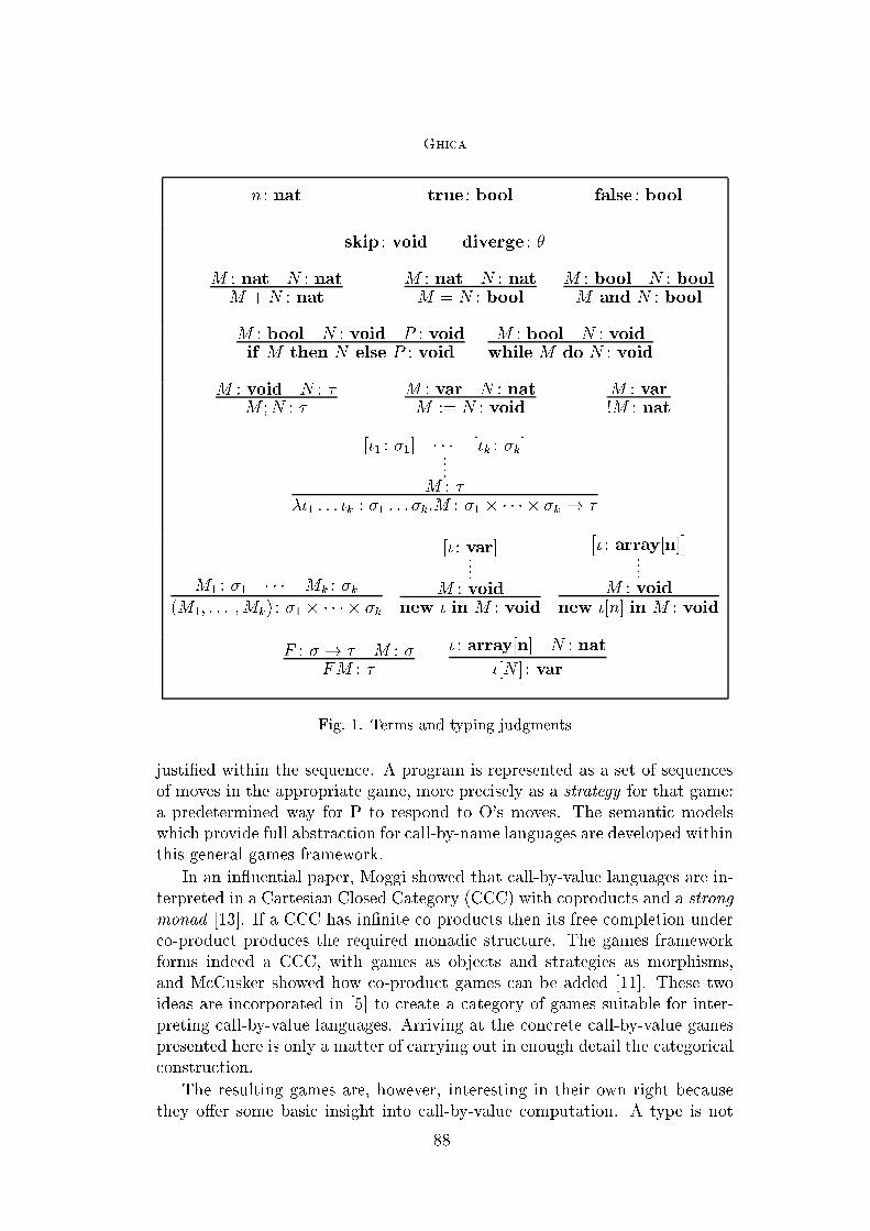
Ghica

n : nat true : bool false : bool

skip : void diverge : �

M : nat N : natM +N : nat

M : nat N : natM = N : bool

M : bool N : boolM and N : bool

M : bool N : void P : voidif M then N else P : void

M : bool N : voidwhile M do N : void

M : void N : �M ;N : �

M : var N : natM := N : void

M : var!M : nat

[�1 : �1] � � � [�k : �k]....

M : ���1 : : : �k : �1 : : : �k:M : �1 � � � � � �k ! �

M1 : �1 � � � Mk : �k(M1; : : : ;Mk) : �1 � � � � � �k

[� : var]....

M : voidnew � in M : void

�� : array[n]

�....

M : voidnew �[n] in M : void

F : � ! � M : �FM : �

� : array[n] N : nat

�[N ] : var

Fig. 1. Terms and typing judgments

justi�ed within the sequence. A program is represented as a set of sequences

of moves in the appropriate game, more precisely as a strategy for that game:

a predetermined way for P to respond to O's moves. The semantic models

which provide full abstraction for call-by-name languages are developed within

this general games framework.

In an in uential paper, Moggi showed that call-by-value languages are in-

terpreted in a Cartesian Closed Category (CCC) with coproducts and a strong

monad [13]. If a CCC has in�nite co-products then its free completion under

co-product produces the required monadic structure. The games framework

forms indeed a CCC, with games as objects and strategies as morphisms,

and McCusker showed how co-product games can be added [11]. These two

ideas are incorporated in [5] to create a category of games suitable for inter-

preting call-by-value languages. Arriving at the concrete call-by-value games

presented here is only a matter of carrying out in enough detail the categorical

construction.

The resulting games are, however, interesting in their own right because

they o�er some basic insight into call-by-value computation. A type is not

88

Ghica

represented by a game, but by a family of games. A strategy interpreting a

term has two distinct stages, a protocol stage in which one of the members

of the family is selected, followed by a play in the selected game. Intuitively,

this mirrors the fact that, in call-by-value, all arguments are evaluated exactly

once before the body of the function is evaluated. Accordingly, free identi�ers

can have only one value throughout the evaluation of a term. In contrast, call-

by-name allows identi�ers to correspond to di�erent values at various points

in the evaluation.

This point is illustrated by the following example: f : nat! nat; x: nat `

f(x) : nat. For call-by-name a typical play is:

f : nat ! nat x: nat ` f(x) : nat

qq

qqn

nq

qn0

n0

mm

O asks for the value of f(x); P asks for the value returned by f; O asks for the

argument of f; P asks for the value of x; O answers n; P relays that answer

back to O; O asks again for the argument of f and the same cycle repeats; O

answers with m to the value returned by f; P relays that answer back to O,

answering the initial question. Notice that in the course of the play the value

of x can be requested several times, and since the answer is given by O it may

change. Now let us look at the same term evaluated under call-by-value:

f : nat ! nat x: nat ` f(x) : nat

?

?

n?(n)

?(n)m

m

The moves under the ` symbol are not part of the play, but they are some

of the concealed activities that are part of the protocol. The play is: O asks

for the value of f(x); as a result of the protocol, P asks for the value of f in

component n; O answers m; P relays the answer back, answering the initial

question. Only part of the protocol is shown: P asks in what component should

89

Ghica

the play proceed; O answers with a component index n for x; P requests that

the game should continue in component n.

In [5] it was shown that this games framework gives a fully abstract model

for call-by-value. Moreover, by relaxing one of the constraints on strategies

(innocence) the same article shows how a fully abstract model for an imper-

ative language with ML-style data references can be de�ned, using a good-

variable non-innocent strategy to model mutable store. These ideas are fur-

ther expanded in [1] to show that dropping another constraint on strategies

(visibility) gives rise to a fully abstract model for general references (references

to data, procedures, higher order functions, other references).

4 Regular language semantics of types

A game for a type, or a strategy for a term, is fully characterized by its

set of plays together with the way moves are justi�ed. But if the language is

suÆciently restricted then there is only one way in which moves can be justi�ed

within a play sequence|Foil is such a restricted language. This means that

such languages can be fully characterized by plays taken to be sequences of

moves only. Moreover, the sequences of moves are regular sets, so they can

be denoted by (extended) regular expressions. This is an approach we took

before, in dealing with Algol [7]. For the restricted language, extended regular

expressions give a convenient, compact, fully formal calculus, quite handy in

de�ning the semantics of actual programs. The regular-language semantics

arises out of the model in [5], by working out the details of the categorical

construction.

De�nition 4.1 The set RA of extended regular expressions R over a �nite

alphabet A is de�ned as:

R ::= ; j � j a; a 2 A Constants;

R ::= R �R j R +R j R \ R Operators;

R ::= R� Iteration;

R ::= RjA0; A0 � A Hiding;

R ::= Rhvi Indexing:

Most of the above are standard regular expression constructs, to which we

add intersection and two new operations, hiding and indexing. The latter are

operations on regular languages that can be carried out directly at the level

of regular expressions. Hiding represents a restriction of a regular expression

to a subset of its alphabet by removing all the occurrences of symbols in

the restricted alphabet; its language is the set of sequences of the original

languages with all the elements of A0deleted. Indexing is de�ned as the

tagging of the �rst symbol a of any sequence in the language with the string

90

Ghica

J�K = �Pc2C�P c�

��P

k2K�R�(k)

�; where:

J�K : P v� = ? � v; R� = �; K� = f?g; Cvoid = f?g

Cnat = f0; 1; : : : ; nNg = N; Cbool = ftt ;� g

J�1 � �2K : P c�1��2

= ? � c; C�1��2 = C�1 � C�2

R�1��2(k) =

(R�1(k) if k 2 K�1

R�2(k) if k 2 K�2

; K�1��2 = K�1 ]K�2

JvarK : Pvar = ? � ?; Cvar = f?g; Kvar = N [ f?g

Rvar =P

m2N read �m +

Pm2N write(m)�?

qarray[n]

y: Parray[n] = ? � ?; Carray[n] = f?g

Karray[n] = fiji < ng [ fiji < ng �N

Rarray[n] =P

m2Ni<n

read(i)�m +

Pm2Ni<n

write(i;m)�?

J� ! �K : P�!� = ? � ?; C�!� = f?g

R�!� =

Pc2K�!�

�q(c) �

Pd2C�

R�hci � d��; K�!� = C�

Fig. 2. Semantics of Foil types

v, resulting in a(uv), where u is the pre-existing tag of R, possibly empty (�).

A regular-language representation of the game semantics of Foil is de�ned

as follows. With types we associate games, represented as regular languages

over an alphabet denoting the moves. With terms we associate strategies,

represented as regular languages over the disjoint sum of the alphabets of the

types of the free identi�ers and the term itself.

As mentioned in the previous sections, a call-by-value game for a type

� has two stages: a protocol-game P c� followed by a component-game R� =P

k2K�R�(k). The protocol part of the play corresponds to the co-product

structure which forms the monad, tying together the various components.

A play in the protocol game always has the form ? � c for c 2 C�. We

call C� the set of component-selecting moves. The �rst move in a play in

the component game R� has the form m(k), where k 2 K�. We call K� the

set of component-de�ning moves; every such component is represented by the

regular language R�(k). Notice that C� and K� are distinct sets. If sets C or

K only have one element (?), we will often omit it as an index.

The regular language semantics of Foil types is the one given in Figure 2.

For void, nat and bool the de�nition is straightforward. Variables var are

the product of an acceptor and an expression type, not rei�ed in the actual

language. Arrays of size n are identi�ed with products of n variables. Proving

91

Ghica

these regular expressions correctly represent games is tedious, but routine.

In the case of product and function types it is required that the alphabets

(sets of moves) of the types involved are disjoint. This is achieved by system-

atically tagging all the moves in each alphabet with tags uniquely associated

with each type occurrence.

5 Regular language semantics of terms

Terms in Foil are interpreted as families of regular expressions, representing

the call-by-value strategies. They have the following form, where P and R are

the protocol and the component parts:

J�1 : �1; : : : ; �n : �n `M : �K =]

c2Q

i�nC�i

nPk2K�

Pc;k

M �RM(k)�o:

Free identi�ers are interpreted as:

J� : � ` � : �K : Pc;k

� : � = P c� ; k 2 K�; R� = R�[m=m�m�

][n=n��n];

for all moves m of odd index in the play (the O-moves) and n of even index

(P-moves). Since in the regular expressions moves always occur in pairs, this

substitution can be carried out directly on the regular expression de�ning the

plays. This \doubling-up" of moves is the representation of the important

copy-cat strategy of game semantics. The new tag � is meant to di�erentiate

between the two occurrences of type �, in the environment and in the term

itself. For example:

Jx: nat ` x: natK= f? � n � � j n 2 Ng ;

Jf : nat! nat ` f : nat! natK=�?�?�R�f

=

n?�?�

�Pi;n2Nq(i)�q(i)

f�nf �n

��o:

For all basic constants of the language we have R = � and:

Pn : nat = ? � n; Ptrue : bool = ? � tt ; Pdiverge : � = ;;

Pskip : void = ? � ?; Pfalse : bool = ? � � :

Binary arithmetic, logic and arithmetic-logic operators can be interpreted as

abbreviations involving prede�ned functions, for which the semantics of ap-

plication (to be de�ned later) will be used to compose the meanings of sub-

phrases:

J+: nat� nat! natK : Pm;n+

= ? � ?; R+(m;n) = ?(m;n)�(m + n);

with m;n 2 N . Similarly for all other operators. Sequencing is:

92

Ghica

J�;� : void� void! voidK : P; = ? � ?; R; = �;

J�;� : void� nat! natK : P; =

Xn2N

? � n; R; = �:

Assignment and dereferencing are respectively:

J�:=� : var� nat! voidK : P n:=

= ? � ?; R:=(n) = write(n)�?;

J!� : var! natK : P! = ? � ?; R! =

Xn2N

read �n:

Abstraction is de�ned as explicitly reindexing the regular expressions denoting

the meaning of a termM with the component moves of the types of identi�ers

abstracted over:

J� ` ��1 : : : �k : �1 � � � � � �k:M : �1 � � � � � �k ! �K :P k� = ? � ?; R�(k) = Qhki; k 2

Yi�n

C�i ; Q 2 J�; �1 : �1; : : : ; �k : �k `MK :

The most important, and the most complex, is the meaning of application:

J� `MN : �K : PMN = ?�P c0

N �R0M(c)[x�y=R

x;y

N ]; RMN = �

where ?�P c0

N �c�RN 2 J�00 ` N : �K ; RN =

Xx;y

x�Rx;y

N �y

?�?�Xc

q(c)�R0M(c) 2 J�0 `M : � ! �K ; R� =

Xx;y

x�y:

The regular expressions and regular expression families involved in the de�ni-

tion above are well de�ned in general, with one exception. If N is a diverging

term then either one of P c0

N and RN may be ; with the other arbitrary, ;

being a zero-element for concatenation. This ambiguity is resolved by always

choosing P c0

N = ;, to be consistent with the fact that Pdiverge = ;, as presented

earlier. The choice for RN is then irrelevant, � by convention.

The semantics of application is derived directly from the game semantics

as well, more precisely from compositions of strategies. In composing strate-

gies, which is how application is interpreted, the moves in the game (type

occurrence) through which composition is realized serve as \triggers" which

switch the thread of execution between the two strategies. In our particular

case, whenever such a move x occurs, a regular expression denoting the trace

of execution for the argument is inserted in the regular expression denoting

the body of the function, up to the point where another context-switching

move y occurs. In the process of composing strategies all trigger moves are

subsequently hidden. Here, the key technique is to decompose a regular ex-

pression into smaller regular expressions and, using systematic substitution

and concatenation, create the regular expressions corresponding to the result.

This technique will be also used in de�ning the regular language semantics of

terms which are not abbreviations.

Since functions are not curried we need to de�ne pairing. It re ects the

left-to-right order of argument evaluation in function call, speci�c to Foil:

93

Ghica

q� ` (M;N) : � � �0

y:

P(c;c0)(k;k0)

M;N = ?�Qc;k

M �Qc0;k0

N �(c; c0); RM;N(k; k0) =

�RM(k) +RN(k

0)

��where P

c;k

M = ?�Qc;k

M �c; Pc;k0

N = ?�Qc0;k0

N �c0:

Branching and looping are de�ned directly, not as abbreviations:

Jif B then M else NK : Pif = (?�P ttB �P

0M �?) + (?�P

�B �P

0N �?); Rif = �;

Jwhile B do MK : Pwhile = ?�(P ttB �P

0M)

��P

�B �?; Rwhile = �;

where : PB =

Xv2ftt ;� g

?�P vB�v; PM = ?�P 0

M �?; PN = ?�P 0N �? :

The semantics of if is directly speci�ed in the games semantics. Looping in

game semantics is de�ned as an abbreviation using the recursion combinator.

A general recursion combinator is not speci�ed in this treatment, but the �xed

point can be calculated by hand; the semantics of while above is the result

of that calculation.

Array element access is also directly de�ned:

J� ` �[N ] : varK :

P k�[N ]

= ?�P k0

N �?; R�[N ](k) =Xm2N

read(k)�m+

Xm2N

write(k;m)�?;

where P k0

N = ?�P kN �k:

Finally, as in the case of Algol, local variables are realized by imposing a

good variable restriction on the plays and by hiding the actions of the local

variables. Good-variable behaviour simply means that the last value written

in a variable will be the next value read from that variable; this restriction

is imposed using intersection with the following regular expression, associated

with a variable �:

� = A�

��

�A�

��P

n2Nwrite(n)��?��A�

��(read ��n��A�

�)���

;

where A� = fread �;write(n)�; n�; ?�jn 2 Ng is the set of all moves tagged by �,

i.e. all moves involving variable �. Therefore local variable de�nition is:

Jnew � in MK = f( � \Q) jA�jQ 2 JMKg :

For similar reasons, the meaning of array declaration is:

Jnew �[n] in MK =(�\

i�n

�[i] \Q

�����Si�n

A�[i]

�����Q 2 JMK);

�[i] = A�[i]

��

�A�[i]

��P

n2Nwrite(n; i)��?��A�[i]

��(read(i)��n��A�[i]

�)���

; i � n:

This concludes the semantic de�nition of Foil. We can state that:

Lemma 5.1 (Representation) The regular language semantics of Foil is

a fully correct representation of the games and strategies used in the game

semantic model.

94

Ghica

From this, it follows directly from [5] that:

Theorem 5.2 (Full Abstraction) The regular language semantics of Foil

is fully abstract, i.e. two terms of Foil are equivalent if and only if they denote

the same family of regular languages:

For all � ` P;Q : �; P � Q() JP K = JQK :In addition, since the representation is by regular languages, for which

language equality is decidable, it follows directly that:

Theorem 5.3 (Decidability) Equivalence of two terms of Foil is decidable.

6 Example of reasoning

Since one of the stated purposes of this article is to provide a basis for a new

and potentially practical tool, we think it is important to show in some detail

an example. Space constraints prevent us from presenting a realistic program,

so we will instead prove a simple, but theoretically important, equivalence of

Foil:

f : nat! void; v : nat ` new x in x := v; f(!x) �void f(v):

Proof:

Jx: var ` x: varK : Px = ? � ?;

Rx =

Xn2N

read �readx�nx�n +

Xm2N

write(m)�write(m)x�?x�?

Jx: var `!x : natK : P!x = ?�

Xn2N

�readx�nx�n; R!x = �

Jf : nat! void ` f : nat! voidK : Pf = ?�?; Rf =

�Pi2Nq(i)�q(i)

f�?f �?

��

Jf : nat! void; x: var ` f(!x) : natK :Pf(!x) = ?�

Xn2N

readx�nx��q(n)f �?f

���?; Rf(!x) = �

Jv : nat; x: var ` x := v: voidK : P vx:=v = ?�write(v)x� ?x �?; Rx:=v = �

Jf : nat! void; v : nat; x: var ` x := v; f(!x) : voidK :P vx:=v;f(!x) = ?�write(v)x�?x�

Xn2N

readx�nx��q(n)f �?f

���?; Rx:=v;f(!x) = �

95

Ghica

Jf : nat! void; v : nat ` new x in x := v; f(!x) : voidK :P v

= ?� write(v)x� ?x �readx�vx��q(v)f �?f

���? = ?�

�q(v)f �?f

���?; R = �:

Therefore:

Jf : nat! void; v : nat ` new x in x := v; f(!x) : voidK=

n?��q(v)f �?f

��� ?��v 2 N

o= Jf : nat! void; v : nat ` f(v) : voidK :

7 Conclusion

We have presented a games-based regular language semantics for an imperative

language with �rst order procedures using call-by-value function application,

with arrays and variables passed by-reference. The model is obtained directly

from the game semantic model [5,1] by working out the details of the category-

theoretical presentation and by observing that much of the games apparatus

(justi�cation pointers, etc.) is unnecessary in handling the present language

subset. Two important and useful features of imperative programs with pro-

cedures, recursion and pointers, are omitted. A �xed-point combinator can

not be de�ned using regular languages only, but �xed points of functions can

be calculated \by hand," as we did in dealing with the while construct. Data

pointers also can not be represented directly using the present formalism, but

they could be in principle encoded using arrays and array indices|but this

method has limitations.

Acknowledgement

Guy McCusker's suggestions and explanations were essential in the writing of

this paper, I owe him a great deal. I would like to thank Bob Tennent for his

support and encouragement. Many thanks are due to the anonymous referees

for providing insightful comments and pertinent corrections.

References

[1] Abramsky, S., K. Honda and G. McCusker, A fully abstract game semantics

for general references, in: Proceedings, Thirteenth Annual IEEE Symposium on

Logic in Computer Science, 1998.

[2] Abramsky, S., P. Malacaria and R. Jagadeesan, Full abstraction for PCF,

Lecture Notes in Computer Science 789 (1994), pp. 1{59.

[3] Abramsky, S. and G. McCusker, Game semantics, lecture notes, 1997

Marktoberdorf summer school (available from http://www.dcs.ed.ac.uk/

home/samson/mdorf97.ps.gz).

96

Ghica

[4] Abramsky, S. and G. McCusker, Linearity, sharing and state: a fully abstract

game semantics for Idealized Algol with active expressions, in: O'Hearn and

Tennent [14] pp. 297{329, two volumes.

[5] Abramsky, S. and G. McCusker, Call-by-value games, in: CSL: 11th Workshop

on Computer Science Logic, LNCS 1414, 1998, pp. 1{17.

[6] Abramsky, S. and G. McCusker, Full abstraction for Idealized Algol with passive

expressions, Theoretical Computer Science 227 (1999), pp. 3{42.

[7] Ghica, D. R. and G. McCusker, Reasoning about idealized algol using regular

languages, in: Proceedings of 27th International Colloquium on Automata,

Languages and Programming ICALP 2000, LNCS 1853 (2000), pp. 103{116.

[8] Hankin, C. and P. Malacaria, Generalised owcharts and games, Lecture Notes

in Computer Science 1443 (1998).

[9] Hankin, C. and P. Malacaria, Non-deterministic games and program analysis:

an application to security, in: Proceedings, Fourteenth Annual IEEE Symposium

on Logic in Computer Science, 1999 pp. 443{452.

[10] Hyland, J. M. E. and C.-H. L. Ong, On full abstraction for PCF: I, II and III,

Information and Computation 163 (2000).

[11] McCusker, G., \Games and Full Abstraction for a Functional Metalanguage

with Recursive Types," Distinguished Dissertations, Springer-Verlag Limited,

1998.

[12] Meyer, A. R. and K. Sieber, Towards fully abstract semantics for local

variables: preliminary report, in: Conference Record of the Fifteenth Annual

ACM Symposium on Principles of Programming Languages (1988), pp. 191{

203, reprinted as Chapter 7 of [14].

[13] Moggi, E., Notions of computation and monads, Information and Computation

93 (1991), pp. 55{92.

[14] O'Hearn, P. W. and R. D. Tennent, editors, \Algol-like Languages," Progress

in Theoretical Computer Science, Birkh�auser, Boston, 1997, two volumes.

[15] Schmidt, D. A., On the need for a popular formal semantics, ACM SIGPLAN

Notices 32 (1997), pp. 115{116.

97

98

MFPS 17 Preliminary Version

Typing Correspondence Assertions forCommunication Protocols

Andrew D. Gordon

Microsoft Research, Cambridge

Alan Je�rey

DePaul University, Chicago

Abstract

Woo and Lam propose correspondence assertions for specifying authenticity proper-

ties of security protocols. The only prior work on checking correspondence assertions

depends on model-checking and is limited to �nite-state systems. We propose a de-

pendent type and e�ect system for checking correspondence assertions. Since it

is based on type-checking, our method is not limited to �nite-state systems. This

paper presents our system in the simple and general setting of the �-calculus. We

show how to type-check correctness properties of example communication protocols

based on secure channels. In a related paper, we extend our system to the more

complex and speci�c setting of checking cryptographic protocols based on encrypted

messages sent over insecure channels.

1 Introduction

Correspondence Assertions To a �rst approximation, a correspondence

assertion about a communication protocol is an intention that follows the

pattern:

If one principal ever reaches a certain point in a protocol, then some other

principal has previously reached some other matching point in the protocol.

We record such intentions by annotating the program representing the

protocol with labelled assertions of the form beginL or endL. These assertions

have no e�ect at runtime, but notionally indicate that a principal has reached

a certain point in the protocol. The following more accurately states the

intention recorded by these annotations:

If the program embodying the protocol ever asserts end L, then there is a

distinct previous assertion of begin L.

This is a preliminary version. The �nal version will be published inElectronic Notes in Theoretical Computer Science

URL: www.elsevier.nl/locate/entcs

Gordon and Jeffrey

Woo and Lam [23] introduce correspondence assertions to state intended

properties of authentication protocols based on cryptography. Consider a

protocol where a principal a generates a new session key k and transmits it

to b. We intend that if a run of b ends a key exchange believing that it has

received key k from a, then a generated k as part of a key exchange intended

for b. We record this intention by annotating a's generation of k by the label

begin ha; b; ki, and b's reception of k by the label end ha; b; ki.

A protocol can fail a correspondence assertion because of several kinds of

bug. One kind consists of those bugs that cause the protocol to go wrong

without any external interference. Other kinds are bugs where an unreliable

or malicious network or participant causes the protocol to fail.

This Paper We show in this paper that correctness properties expressed by

correspondence assertions can be proved by type-checking. We embed corre-

spondence assertions in a concurrent programming language (the �-calculus

of Milner, Parrow, and Walker [17]) and present a new type and e�ect system

that guarantees safety of well-typed assertions. We show several examples of

how correspondence assertions can be proved by type-checking.

Woo and Lam's paper introduces correspondence assertions but provides

no techniques for proving them. Clarke and Marrero [4] use correspondence

assertions to specify properties of e-commerce protocols, such as authoriza-

tions of transactions. To the best of our knowledge, the only previous work

on checking correspondence assertions is a project by Marrero, Clarke, and

Jha [16] to apply model-checking techniques to �nite state versions of security

protocols. Since our work is based on type-checking, it is not limited to �nite

state systems. Moreover, type-checking is compositional: we can verify com-

ponents in isolation, and know that their composition is safe, without having

to verify the entire system. Unlike Marrero, Clarke, and Jha's work, however,

the system of the present paper does not deal with cryptographic primitives,

and nor does it deal with an arbitrary opponent. Still, in another paper [9],

we adapt our type and e�ect system to the setting of the spi-calculus [1],

an extension of the �-calculus with abstract cryptographic primitives. This

adaptation can show, moreover, that properties hold in the presence of an

arbitrary untyped opponent.

Review of The Untyped �-Calculus Milner, Parrow, and Walker's �-

calculus is a concurrent formalism to which many kinds of concurrent com-

putation may be reduced. Its simplicity makes it an attractive vehicle for

developing the ideas of this paper, while its generality suggests they may be

widely applicable. Its basic data type is the name, an unguessable identi�er

for a communications channel. Computation is based on the exchange of mes-

sages, tuples of names, on named channels. Programming in the �-calculus

is based on the following constructs (written, unusually, with keywords, for

100

Gordon and Jeffrey

the sake of clarity). The rest of the paper contains many examples. An out-

put process out xhy1; : : : ; yni represents a message hy1; : : : ; yni sent on the

channel x. An input process inp x(z1; : : : ; zn);P blocks till it �nds a mes-

sage sent on the channel x, reads the names in the message into the variables

z1; : : : ; zn, and then runs P . The process P j Q is the parallel composition of

the two processes P and Q; the two may run independently or communicate

on shared channels. The name generation process new(x);P generates a fresh

name, calls it x, then runs P . Unless P reveals x, no other process can use

this fresh name. The replication process repeat P behaves like an unbounded

parallel array of replicas of P . The process stop represents inactivity; it does

nothing. Finally, the conditional if x = y then P else Q compares the names

x and y. If they are the same it runs P ; otherwise it runs Q.

2 Correspondence Assertions, by Example

This section introduces the idea of de�ning correspondence assertions by an-

notating code with begin- and end-events. We give examples of both safe code

and of unsafe code, that is, of code that satis�es the correspondence assertions

induced by its annotations, and of code that does not.

A transmit-acknowledge handshake is a standard communications idiom,

easily expressed in the �-calculus: along with the actual message, the sender

transmits an acknowledgement channel, upon which the receiver sends an

acknowledgement. We intend that:

During a transmit-acknowledge handshake, if the sender receives an ac-

knowledgment, then the receiver has obtained the message.

Correspondence assertions can express this intention formally. Suppose

that a and b are the names of the sender and receiver, respectively. We

annotate the code of the receiver b with a begin-assertion at the point after

it has received the message msg. We annotate the code of the sender a with

an end-assertion at the point after it has received the acknowledgement. We

label both assertions with the names of the principals and the transmitted

message, ha; b;msgi. Hence, we assert that if after sending msg to b, the

sender a receives an acknowledgement, then a distinct run of b has received

msg.

Suppose that c is the name of the channel on which principal b receives

messages from a. Here is the �-calculus code of the annotated sender and

receiver:

Rcver(a; b; c)�

=

inp c(msg; ack);

begin ha; b;msgi;

out ackhi

Snder(a; b; c)�

=

new(msg); new(ack);

out chmsg; acki; inp ack();

end ha; b;msgi

The sender creates a fresh message msg and a fresh acknowledgement channel

101

Gordon and Jeffrey

ack , sends the two on the channel c, waits for an acknowledgement, and then

asserts an end-event labelled ha; b;msgi.

The receiver gets the message msg and the acknowledgement channel ack

o� c, asserts a begin-event labelled ha; b;msgi, and sends an acknowledgement

on ack .

We say a program is safe if it satis�es the intentions induced by the begin-

and end-assertions. More precisely, a program is safe just if for every run of

the program and for every label L, there is a distinct begin-event labelled L

preceding every end-event labelled L. (We formalize this de�nition in Sec-

tion 5.)

Here are three combinations of our examples: two safe, one unsafe.

new(c);

Snder(a; b; c) jRcver(a; b; c)

(Example 1: safe)

Example 1 uses one instance of the sender and one instance of the receiver

to represent a single instance of the protocol. The restriction new(c); makes

the channel c private to the sender and the receiver. This assembly is safe; its

only run correctly implements the handshake protocol.

new(c);

Snder(a; b; c) j

Snder(a; b; c) jrepeat Rcver(a; b; c)

(Example 2: safe)

Example 2 uses two copies of the sender|representing two attempts by a single

principal a to send a message to b|and a replicated copy of the receiver|

representing the principal b willing to accept an unbounded number of mes-

sages. Again, this assembly is safe; any run consists of an interleaving of two

correct handshakes.

new(c);

Snder(a; b; c) j

Snder(a0; b; c) jrepeat Rcver(a; b; c)

(Example 3: unsafe)

Example 3 is a variant on Example 2, where we keep the replicated receiver

b, but change the identity of one of the senders, so that the two senders

represent two di�erent principals a and a0. These two principals share a single

channel c to the receiver. Since the identity a of the sender is a parameter

of Rcver(a; b; c) rather than being explicitly communicated, this assembly is

unsafe. There is a run in which a0 generates msg and ack , and sends them to b;

b asserts a begin-event labelled ha; b;msgi and outputs on ack ; then a0 asserts

an end-event labelled ha0; b;msgi. This end-event has no corresponding begin-

event so the assembly is unsafe, re ecting the possibility that the receiver can

102

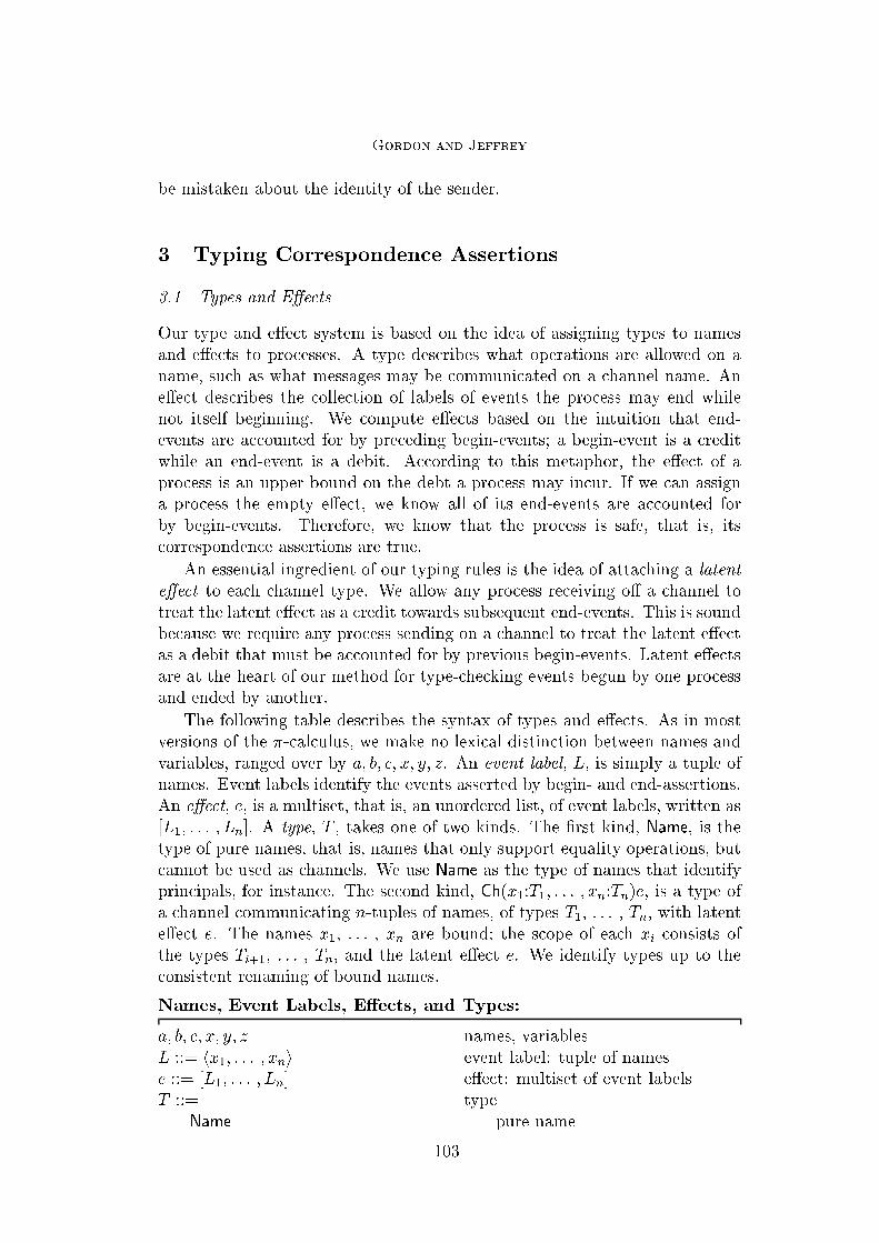
Gordon and Jeffrey

be mistaken about the identity of the sender.

3 Typing Correspondence Assertions

3.1 Types and E�ects

Our type and e�ect system is based on the idea of assigning types to names

and e�ects to processes. A type describes what operations are allowed on a

name, such as what messages may be communicated on a channel name. An

e�ect describes the collection of labels of events the process may end while

not itself beginning. We compute e�ects based on the intuition that end-

events are accounted for by preceding begin-events; a begin-event is a credit

while an end-event is a debit. According to this metaphor, the e�ect of a

process is an upper bound on the debt a process may incur. If we can assign

a process the empty e�ect, we know all of its end-events are accounted for

by begin-events. Therefore, we know that the process is safe, that is, its

correspondence assertions are true.

An essential ingredient of our typing rules is the idea of attaching a latent

e�ect to each channel type. We allow any process receiving o� a channel to

treat the latent e�ect as a credit towards subsequent end-events. This is sound

because we require any process sending on a channel to treat the latent e�ect

as a debit that must be accounted for by previous begin-events. Latent e�ects

are at the heart of our method for type-checking events begun by one process

and ended by another.

The following table describes the syntax of types and e�ects. As in most

versions of the �-calculus, we make no lexical distinction between names and

variables, ranged over by a; b; c; x; y; z. An event label, L, is simply a tuple of

names. Event labels identify the events asserted by begin- and end-assertions.

An e�ect, e, is a multiset, that is, an unordered list, of event labels, written as

[L1; : : : ; Ln]. A type, T , takes one of two kinds. The �rst kind, Name, is the

type of pure names, that is, names that only support equality operations, but

cannot be used as channels. We use Name as the type of names that identify

principals, for instance. The second kind, Ch(x1:T1; : : : ; xn:Tn)e, is a type of

a channel communicating n-tuples of names, of types T1, : : : , Tn, with latent

e�ect e. The names x1, : : : , xn are bound; the scope of each xi consists of

the types Ti+1, : : : , Tn, and the latent e�ect e. We identify types up to the

consistent renaming of bound names.

Names, Event Labels, E�ects, and Types:

a; b; c; x; y; z names, variables

L ::= hx1; : : : ; xni event label: tuple of names

e ::= [L1; : : : ; Ln] e�ect: multiset of event labels

T ::= type

Name pure name

103

Gordon and Jeffrey

Ch(x1:T1; : : : ; xn:Tn)e channel with latent e�ect e

For example:

� Ch()[ ], a synchronization channel (that is, a channel used only for synchro-

nization) with no latent e�ect.

� Ch(a:Name)[hbi], a channel for communicating a pure name, costing [hbi] to

senders and paying [hbi] to receivers, where b is a �xed name.

� Ch(a:Name)[hai], a channel for communicating a pure name, costing [hai]

to senders and paying [hai] to receivers, where a is the name communicated

on the channel.

� Ch(a:Name; b:Ch()[hai])[ ], a channel with no latent e�ect for communicating

pairs of the form a; b, where a is a pure name, and b is the name of a syn-

chronization channel, costing [hai] to senders and paying [hai] to receivers.

The following is a convenient shorthand for the lists of typed variable decla-

rations found in channel types:

Notation for Typed Variables:

~x:~T�

= x1:T1; : : : ; xn:Tn where ~x = x1; : : : ; xn and ~T = T1; : : : ; Tn

��

= () the empty list

The following equations de�ne the the sets of free names of our syntax

as follows: variable declarations, fn(�:�)�

= ? and fn(~x:~T ; x:T )�

= fn(~x:~T ) [

(fn(T )�f~xg); types, fn(Name)�

= ? and fn(Ch(~x:~T )e)�

= fn(~x:~T )[(fn(e)�f~xg);

event labels, fn(hx1; : : : ; xni)�

= fx1; : : : ; xng; and events, fn([L1; : : : ; L1])�

=

fn(L1) [ � � � [ fn(Ln).

For any of these forms of syntax, we write �fx yg for the operation of

capture-avoiding substitution of the name y for each free occurrence of the

name x. We write �f~x ~yg, where ~x = x1; : : : ; xn and ~y = y1; : : : ; yn for the

iterated substitution �fx1 y1g � � � fxn yng.

3.2 Syntax of our Typed �-Calculus

We explained the informal semantics of begin- and end-assertions in Section 2,

and of the other constructs in Section 1.

Processes:

P;Q;R ::= process

out xhy1; : : : ; yni polyadic asynchronous output

inp x(y1:T1; : : : ; yn:Tn);P polyadic input

if x = y then P else Q conditional

new(x:T );P name generation

P j Q composition

repeat P replication

104

Gordon and Jeffrey

stop inactivity

begin L;P begin-assertion

end L;P end-assertion

There are two name binding constructs: input and name generation. In

an input process inp x(y1:T1; : : : ; yn:Tn);P , each name yi is bound, with scope

consisting of Ti+1, : : : , Tn, and P . In a name restriction new(x:T );P , the

name x is bound; its scope is P . We write Pfx yg for the outcome of a

capture-avoiding substitution of the name y for each free occurrence of the

name x in the process P . We identify processes up to the consistent renaming

of bound names. We let fn(P ) be the set of free names of a process P . We

sometimes write an output as out xh~yi where ~y = y1; : : : ; yn, and an input

as inp x(~y:~T );P , where ~y:~T is a variable declaration written in the notation

introduced in the previous section. We write out xh~yi;P as a shorthand for

out xh~yi j P .

3.3 Intuitions for the Type and E�ect System

As a prelude to our formal typing rules, we present the underlying intuitions.

Recall the intuition that end-events are costs to be accounted for by begin-

events. When we say a process P has e�ect e, it means that e is an upper

bound on the begin-events needed to precede P to make the whole process

safe. In other words, if P has e�ect [L1; : : : ; Ln] then beginL1; � � � ; beginLn;P

is safe.

Typing Assertions An assertion beginL;P pays for one end-event labelled

L in P ; so if P is a process with e�ect e, then begin L;P is a process with

e�ect e�[L], that is, the multiset e with one occurrence of L deleted. So we

have a typing rule of the form:

P : e ) begin L;P : e�[L]

If P is a process with e�ect e, then endL;P is a process with e�ect e+[L],

that is, the concatenation of e and [L]. We have a rule:

P : e ) end L;P : e+[L]

Typing Name Generation and Concurrency The e�ect of a name gen-

eration process new(x:T );P , is simply the e�ect of P . To prevent scope con-

fusion, we forbid x from occurring in this e�ect.

P : e; x =2 fn(e) ) new(x:T );P : e

The e�ect of a concurrent composition of processes is the multiset union

of the constituent processes.

P : eP ; Q : eQ ) P j Q : eP+eQ

The inactive process asserts no end-events, so its e�ect is empty.

105

Gordon and Jeffrey

stop : [ ]

The replication of a process P behaves like an unbounded array of repli-

cas of P . If P has a non-empty e�ect, then its replication would have an

unbounded e�ect, which could not be accounted for by preceding begin-

assertions. Therefore, to type repeat P we require P to have an empty e�ect.

P : [ ] ) repeat P : [ ]

Typing Communications We begin by presenting the rules for typing

communications on monadic channels with no latent e�ect, that is, those with

types of the form Ch(y:T )[ ]. The communicated name has type T . An output

out xhzi has empty e�ect. An input inp x(y:T );P has the same e�ect as P .

Since the input variable in the process and in the type are both bound, we

may assume they are the same variable y.

x : Ch(y:T )[ ]; z : T ) out xhzi : [ ]x : Ch(y:T )[ ]; P : e; y =2 fn(e) ) inp x(y:T );P : e

Next, we consider the type Ch(y:T )e` of monadic channels with latent e�ect

e`. The latent e�ect is a cost to senders, a bene�t to receivers, and is the scope

of the variable y. We assign an output out xhzi the e�ect e`fy zg, wherewe have instantiated the name y bound in the type of the channel with z,

the name actually sent on the channel. We assign an input inp x(y:T );P the

e�ect e� e`, where e is the e�ect of P . To avoid scope confusion, we require

that y is not free in e� e`.

x : Ch(y:T )e`; z : T ) out xhzi : e`fy zgx : Ch(y:T )e`; P : e; y =2 fn(e� e`) ) inp x(y:T );P : e� e`

The formal rules for input and output in the next section generalize these

rules to deal with polyadic channels.

Typing Conditionals When typing a conditional if x = y then P else Q,

it is useful to exploit the fact that P only runs if the two names x and y

are equal. To do so, we check the e�ect of P after substituting one for the

other. Suppose then process Pfx yg has e�ect ePfx yg. Suppose also that

process Q has e�ect eQ. Let eP _ eQ be the least upper bound of any two

e�ects eP and eQ. Then eP _eQ is an upper bound on the begin-events needed

to precede the conditional to make it safe, whether P or Q runs. An example

in Section 4.2 illustrates this rule.

Pfx yg : ePfx yg; Q : eQ ) if x = y then P else Q : eP _ eQ

3.4 Typing Rules

Our typing rules depend on several operations on e�ect multisets, most of

which were introduced informally in the previous section. Here are the formal

de�nitions.

106

Gordon and Jeffrey

Operations on e�ects: e+ e0, e � e0, e� e0, L 2 e, e _ e0

[L1; : : : ; Lm] + [Lm+1; : : : ; Lm+n]�

= [L1; : : : ; Lm+n]

e � e0 if and only if e0 = e+ e00 for some e00

e� e0�

= the smallest e00 such that e � e0 + e00

L 2 e if and only if [L] � e

e _ e0�

= the smallest e00 such that e � e00 and e0 � e00

The typing judgments of this section depend on an environment to assign

a type to all the variables in scope.

Environments:

E ::= ~x:~T environment

dom(~x:~T )�

= f~xg domain of an environment

To equate two names in an environment, needed for typing conditionals,

we de�ne a name fusion function. We obtain the fusion Efx x0g from E by

turning all occurrences of x and x0 in E into x0.

Fusing x with x0 in E: Efx x0g

(x1:T1; : : : ; xn:Tn)fx x0g�

=

(x1fx x0g):(T1fx x0g); : : : ; (xnfx x0g):(Tnfx x0g)

where E; x:T�

=

�E if x 2 dom(E)

E; x:T otherwise

The following table summarizes the �ve judgments of our type system,

which are inductively de�ned by rules in subsequent tables. Judgment E ` �

means environment E is well-formed. Judgment E ` T means type T is

well-formed. Judgment E ` x : T means name x is in scope with type T .

Judgment E ` h~xi : h~y:~T i means tuple h~xi matches the variable declaration

~y:~T . Judgment E ` P : e means process P has e�ect e.

Judgments:

E ` � good environment

E ` T good type T

E ` x : T good name x of type T

E ` h~xi : h~y:~T i good message ~x matching ~y:~T

E ` P : e good process P with e�ect e

The rules de�ning the �rst three judgments are standard.

107

Gordon and Jeffrey

Good environments, types, and names:

(Env ?)

? ` �

(Env x)

E ` T x =2 dom(E)

E; x:T ` �

(Type Name)

E ` �

E ` Name

(Type Chan)

E; ~x:~T ` � fn(e) � dom(E) [ f~xg

E ` Ch(~x:~T )e

(Name x)

E 0; x:T;E 00 ` �

E 0; x:T;E 00 ` x : T

The next judgment, E ` h~xi : h~y:~T i, is an auxiliary judgment used for

typing output processes; it is used in the rule (Proc Output) to check that

the message h~xi sent on a channel of type Ch(~y:~T )e matches the variable

declaration ~y:~T .

Good message:

(Msg hi)

E ` �

E ` hi : hi

(Msg x) (where y =2 f~yg [ dom(E))

E ` h~xi : h~y:~T i E ` x : (Tf~y ~xg)

E ` h~x; xi : h~y:~T ; y:T i

Finally, here are the rules for typing processes. The e�ect of a process is an

upper bound; the rule (Proc Subsum) allows us to increase this upper bound.

Intuitions for all the other rules were explained in the previous section.

Good processes:

(Proc Subsum) (where e � e0 and fn(e0) � dom(E))

E ` P : e

E ` P : e0

(Proc Output)

E ` x : Ch(~y:~T )e E ` h~xi : h~y:~T i

E ` out xh~xi : (ef~y ~xg)

(Proc Input) (where fn(e� e0) � dom(E))

E ` x : Ch(~y:~T )e0 E; ~y:~T ` P : e

E ` inp x(~y:~T );P : e� e0

(Proc Cond)

E ` x : T E ` y : T Efx yg ` Pfx yg : ePfx yg E ` Q : eQ

E ` if x = y then P else Q : eP _ eQ

(Proc Res) (where x =2 fn(e))

E; x:T ` P : e

E ` new(x:T );P : e

(Proc Par)

E ` P : eP E ` Q : eQ

E ` P j Q : eP + eQ

108

Gordon and Jeffrey

(Proc Repeat)

E ` P : [ ]

E ` repeat P : [ ]

(Proc Stop)

E ` �

E ` stop : [ ]

(Proc Begin) (where fn(L) � dom(E))

E ` P : e

E ` begin L;P : e� [L]

(Proc End) (where fn(L) � dom(E))

E ` P : e

E ` end L;P : e+ [L]

Section 5 presents our main type safety result, Theorem 5.2, that E ` P : [ ]

implies P is safe. Like most type systems, ours is incomplete. There are safe

processes that are not typeable in our system. For example, we cannot assign

the process if x = x then stop else (end x; stop) the empty e�ect, and yet it is

perfectly safe.

4 Applications

In this section, we present some examples of using correspondence assertions

to validate safety properties of communication protocols. For more examples,

including examples with cryptographic protocols which are secure against ex-

ternal attackers, see the companion paper [9].

4.1 Transmit-Acknowledge Handshake

Recall the untyped sender and receiver code from Section 2. Suppose we make

the type de�nitions:

Msg�

= Name Ack(a; b;msg)�

= Ch()[ha; b;msgi]

Host�

= Name Req(a; b)�

= Ch(msg:Msg ; ack :Ack(a; b;msg))[ ]

109

Gordon and Jeffrey

Suppose also that we annotate the sender and receiver code, and the code of

Example 1 as follows:

Snder(a:Host ; b:Host ; c:Req(a; b))�

=

new(msg:Msg);

new(ack :Ack(a; b;msg));

out chmsg; acki;

inp ack();

end ha; b;msgi

Rcver(a:Host ; b:Host ; c:Req(a; b))�

=

inp c(msg:Msg ; ack :Ack(a; b;msg));

begin ha; b;msgi;

out ackhi

Example1 (a:Host ; b:Host)�

=

new(c:Req(a; b));

Snder(a; b; c) jRcver(a; b; c)

We can then check that a:Host ; b:Host ` Example1 (a; b) : [ ]. Since the system

has the empty e�ect, by Theorem 5.2 it is safe. It is routine to check that

Example 2 from Section 2 also has the empty e�ect, but that Example 3

cannot be type-checked (as to be expected, since it is unsafe).

4.2 Hostname Lookup

In this example, we present a simple hostname lookup system, where a client

b wishing to ping a server a can contact a name server query , to get a network

address ping for a. The client can then send a ping request to the address ping,

and get an acknowledgement from the server. We shall check two properties:

� When the ping client b �nishes, it believes that the ping server a has been

pinged.

� When the ping server a �nishes, it believes that it was contacted by the

ping client b.

We write \a was pinged by b" as shorthand for ha; bi, and \b tried to ping a"

for hb; a; ai. These examples are well-typed, with types which we de�ne later

in this section.

110

Gordon and Jeffrey

We program the ping client and server as follows.

PingClient(a:Hostname; b:Hostname; query :Query)�

=

new(res : Res(a));

out queryha; resi;

inp res(ping : Ping(a));

new(ack : Ack(a; b));

begin \b tried to ping a";

out pinghb; acki;

inp ack();

end \a was pinged by b"

PingServer(a : Hostname; ping : Ping(a))�

=

repeat

inp ping(b : Hostname; ack : Ack(a; b));

begin \a was pinged by b";

end \b tried to ping a";

out ackhi

If these processes are safe, then any ping request and response must come

as matching pairs. In practice, the name server would require some data

structure such as a hash table or database, but for this simple example we

just use a large if-statement:

NameServer(

query :Query ;

h1:Hostname; : : : ; hn:Hostname;

ping1:Ping(h1); : : : ; pingn:Ping(hn)

)�

=

repeat

inp query(h; res);

if h = h1 then out reshping1i else � � �

if h = hn then out reshpingni else stop

To get the system to type-check, we use the following types:

Hostname�

= Name

Ack(a; b)�

= Ch()[\a was pinged by b"]

Ping(a)�

= Ch(b:Hostname; ack :Ack(a; b))[\b tried to ping a"]

Res(a)�

= Ch(ping:Ping(a))[ ]

Query�

= Ch(a:Hostname; res:Res(a))[ ]

111

Gordon and Jeffrey

The most subtle part of type-checking the system is the conditional in the

name server. A typical branch is:

hi : Hostname; ping i : Ping(hi); h : Hostname; res : Res(h)

` if h = hi then out reshping ii else � � � : [ ]

When type-checking the then-branch, (Proc Cond) assumes h = hi by apply-

ing a substitution to the environment:

(hi : Hostname; ping i : Ping(hi); h : Hostname; res : Res(h))fh hig

= (hi : Hostname; ping i : Ping(hi); res : Res(hi))

In this environment, we can type-check the then-branch:

hi : Hostname; pingi : Ping(hi); res : Res(hi)

` out reshpingii : [ ]

If (Proc Cond) did not apply the substitution to the environment, this example

could not be type-checked, since:

hi : Hostname; ping i : Ping(hi); h : Hostname; res : Res(h)

0 out reshping ii : [ ]

4.3 Functions

It is typical to code the �-calculus into the �-calculus, using a return channel

k as the destination for the result. For instance, the hostname lookup example

of the previous section can be rewritten in the style of a remote procedure call.

The client and server are now:

PingClient(a:Hostname; b:Hostname; query :Query)�

=

let (ping : Ping(a)) = query hai;

begin \b tried to ping a";

let () = ping hbi;

end \a was pinged by b"

PingServer(a : Hostname; ping : Ping(a))�

=

fun ping(b:Hostname) f

begin \a was pinged by b";

end \b tried to ping a";

return hi

g

112

Gordon and Jeffrey

The name server is now:

NameServer(

query :Query ;

h1:Hostname; : : : ; hn:Hostname;

ping1:Ping(h1); : : : ; pingn:Ping(hn)

)�

=

fun query(h:Hostname) f

if h = h1 then return hping1i else � � �

if h = hn then return hpingni else stop

g

In order to provide types for these examples, we have to provide a function type

with latent e�ects. These e�ects are precondition/postcondition pairs, which

act like Hoare triples. In the type (~x:~T )e ! (~y:~U)e0 we have a precondition

e which the callee must satisfy, and a postcondition e0 which the caller must

satisfy. For example, the types for the hostname lookup example are:

Ping(a)�

= (b:Hostname)[\b tried to ping a"]! ()[\a was pinged by b"]

Query�

= (a:Hostname)[ ]! (ping:Ping(a))[ ]

which speci�es that the remote ping call has a precondition \b tried to ping a"

and a postcondition \a was pinged by b".

This can be coded into the �-calculus using a translation [17] in continu-

ation passing style.

fun f(~x:~T ) fPg�

= repeat inp f(~x:~T ; k:Ch(~y:~U)e0);P

let (~y:~U) = f h~xi;P�

= new(k:Ch(~y:~U)e0); out fh~x; ki; inp k(~y:~U);P

return h~zi�

= out kh~zi

(~x:~T )e! (~y:~U)e0�

= Ch(~x:~T ; k:Ch(~y:~U)e0)e

This translation is standard, except for the typing. It is routine to verify its

soundness.

5 Formalizing Correspondence Assertions

In this section, we give the formal de�nition of the trace semantics for the

�-calculus with correspondence assertions, which is used in the de�nition of

a safe process. We then state the main result of this paper, which is that

e�ect-free processes are safe.

We give the trace semantics as a labelled transition system. Following

Berry and Boudol [3] and Milner [17] we use a structural congruence P � Q,

and give our operational semantics up to �.

113

Gordon and Jeffrey

Structural Congruence: P � Q

P � P (Struct Re )

Q � P ) P � Q (Struct Symm)

P � Q;Q � R) P � R (Struct Trans)

P � Q) inp x(~y:~T );P � inp x(~y:~T );Q (Struct Input)

P � Q) new(x:T );P � new(x:T );Q (Struct Res)

P � Q) P j R � Q j R (Struct Par)

P � Q) repeat P � repeat Q (Struct Repl)

P j stop � P (Struct Par Zero)

P j Q � Q j P (Struct Par Comm)

(P j Q) j R � P j (Q j R) (Struct Par Assoc)

repeat P � P j repeat P (Struct Repl Par)

new(x:T ); (P j Q) � P j new(x:T );Q (Struct Res Par) (where x =2 fn(P ))

new(x1:T1); new(x2:T2);P �

new(x2:T2); new(x1:T1);P

(Struct Res Res)

(where x1 6= x2; x1 =2 fn(T2); x2 =2 fn(T1))

There are four actions in this labelled transition system:

� Pbegin L����! P 0 when P reaches a begin L assertion.

� Pend L���! P 0 when P reaches an end L assertion.

� Pgen hxi���! P 0 when P generates a new name x.

� P��!P 0 when P can perform an internal action.

For example:

(new(x:Name); begin hxi; end hxi; stop)gen hxi���! (begin hxi; end hxi; stop)begin hxi����! (end hxi; stop)end hxi���! (stop)

Next, we de�ne the syntax of actions �, and their free names and generated

names.

Actions:

�; � ::= actions

begin L begin-event

end L end-event

gen hxi name generation

� internal

114

Gordon and Jeffrey

Free names, fn(�), and generated names, gn(�), of an action �:

fn(�)�

= ? fn(begin L)�

= fn(L) fn(end L)�

= fn(L) fn(gen hxi)�

= fxg

gn(�)�

= ? gn(begin L)�

= ? gn(end L)�

= ? gn(gen hxi�

= fxg

The labelled transition system P��! P 0 is de�ned here.

Transitions: P��! P 0

out xh~xi j inp x(~y);P��!Pf~y ~xg (Trans Comm)

if x = x then P else Q��!P (Trans Match)

if x = y then P else Q��!Q (Trans Mismatch) (where x 6= y)

begin L;Pbegin L����! P (Trans Begin)

end L;Pend L���! P (Trans End)

new(x:T );Pgen hxi���! P (Trans Gen)

P��! P 0 ) P j Q

��! P 0 j Q (Trans Par) (where gn(�) \ fn(Q) = ?)

P��! P 0 ) new(x:T );P

��! new(x:T );P 0 (Trans Res) (where x =2 fn(�))

P � P 0; P 0 ��!Q0; Q0 � Q) P

��!Q (Trans �)

From this operational semantics, we can de�ne the traces of a process, with

reductions Ps�!P 0 where s is a sequence of actions.

Traces:

s; t ::= �1; : : : ; �n trace

Free names, fn(s), and generated names, gn(s), of a trace s:

fn(�1; : : : ; �n)�

= fn(�1) [ � � � [ fn(�n)

gn(�1; : : : ; �n)�

= gn(�1) [ � � � [ gn(�n)

Traced transitions: Ps�!P 0

P � P 0 ) P"�!P 0 (Trace �)

P��! P 00; P 00 s

�!P 0 ) P�;s�! P 0 (Trace Action) (where fn(�) \ gn(s) = ?)

We require a side-condition on (Trace Action) to ensure that generated

names are unique, otherwise we could observe traces such as

(new(x); new(y); stop)gen hxi;gen hxi��������! (stop)

Having formally de�ned the trace semantics of our �-calculus, we can de�ne

when a trace is a correspondence: this is when every end L has a distinct,

115

Gordon and Jeffrey

matching begin L. For example:

begin L; end L is a correspondence

begin L; end L; end L is not a correspondence

begin L; begin L; end L; end L is a correspondence

We formalize this by counting the number of begin L and end L actions there

are in a trace.

Beginnings, begins (�), and endings, ends (�), of an action �:

begins (begin L)�

= [L] ends (begin L)�

= [ ]

begins (end L)�

= [ ] ends (end L)�

= [L]

begins (gen hxi)�

= [ ] ends (gen hxi)�

= [ ]

begins (�)�

= [ ] ends (�)�

= [ ]

Beginnings, begins (s), and endings, ends (s), of a trace s:

begins (�1; : : : ; �n)�

= begins (�1) + � � �+ begins (�n)

ends (�1; : : : ; �n)�

= ends (�1) + � � �+ ends (�n)

Correspondence:

A trace s is a correspondence if and only if ends (s) � begins (s).

A process is safe if every trace is a correspondence.

Safety:

A process P is safe if and only if for all traces s and processes P 0

if Ps�!P 0 then s is a correspondence.

A subtlety of this de�nition of safety is that although we want each end-

event of a safe process to be preceded by a distinct, matching begin-event, a

trace st may be a correspondence by virtue of a later begin-event in t match-

ing an earlier end-event in s. For example, a trace like end L; begin L is a

correspondence.

To see why our de�nition implies that a matching begin-event must precede

each end-event in each trace of a safe process, suppose a safe process has a

trace s; endL; t. By de�nition of traces, the process also has the shorter trace

s; end L, which must be a correspondence, since it is a trace of a safe process.

Therefore, the end-event end L is preceded by a matching begin-event in s.

We can now state the formal result of the paper, Theorem 5.2, that every

e�ect-free process is safe. This gives us a compositional technique for verifying

the safety of communications protocols. It follows from a subject reduction

result, Theorem 5.1. The most diÆcult parts of the formal development to

check in detail are the parts associated with the (Proc Cond) rule, because of

116

Gordon and Jeffrey

its use of a substitution applied to an environment.

Theorem 5.1 (Subject Reduction) Suppose E ` P : e.

(1) If P��!P 0 then E ` P 0 : e.

(2) If Pbegin L����! P 0 then E ` P 0 : e+ [L].

(3) If Pend L���! P 0 then E ` P 0 : e� [L], and L 2 e.

(4) If Pgen hxi���! P 0 and x =2 dom(E) then E; x:T ` P 0 : e for some type T .

Theorem 5.2 (Safety) If E ` P : [ ] then P is safe.

6 Related Work

Correspondence assertions are not new; we have already discussed prior work

on correspondence assertions for cryptographic protocols [23,16]. A contribu-

tion of our work is the idea of directly expressing correspondence assertions

by adding annotations to a general concurrent language, in our case the �-

calculus.

Gi�ord and Lucassen introduced type and e�ect systems [10,15] to manage

side-e�ects in functional programming. There is a substantial literature; recent

applications include memory management for high-level [22] and low-level [5]

languages, race-condition avoidance [7], and access control [20].

Early type systems for the �-calculus [17,19] focus on regulating the data

sent on channels. Subsequent type systems also regulate process behaviour;

for example, session types [21,11] regulate pairwise interactions and linear

types [14] help avoid deadlocks. A recent paper [6] explicitly proposes a type

and e�ect system for the �-calculus, and the idea of latent e�ects on channel

types. This idea can also be represented in a recent general framework for

concurrent type systems [13]. Still, the types of our system are dependent

in the sense that they may include the names of channels; to the best of our

knowledge, this is the �rst dependent type system for the �-calculus. Another

system of dependent types for a concurrent language is Flanagan and Abadi's

system [7] for avoiding race conditions in the concurrent object calculus of

Gordon and Hankin [8].

The rule (Proc Cond) for typing name equality if x = y then P else Q

checks P under the assumption that the names x and y are the same; we

formalize this by substituting y for x in the type environment and the process

P . Given that names are the only kind of value, this technique is simpler

than the standard technique from dependent type theory [18,2] of de�ning

typing judgments with respect to an equivalence relation on values. Honda,

Vasconcelos, and Yoshida [12] also use the technique of applying substitutions

to environments while type-checking.

117

Gordon and Jeffrey

7 Conclusions

The long term objective of this work is to check secrecy and authenticity prop-

erties of security protocols by typing. This paper introduces several key ideas

in the minimal yet general setting of the �-calculus: the idea of expressing

correspondences by begin- and end-annotations, the idea of a dependent type

and e�ect system for proving correspondences, and the idea of using latent

e�ects to type correspondences begun by one process and ended by another.

Several examples demonstrate the promise of this system. Unlike a previous

approach based on model-checking, type-checking correspondence assertions

is not limited to �nite-state systems.

A companion paper [9] begins the work of applying these ideas to crypto-

graphic protocols as formalized in Abadi and Gordon's spi-calculus [1], and

has already proved useful in identifying known issues in published protocols.

Our �rst type system for spi is speci�c to cryptographic protocols based on

symmetric key cryptography. Instead of attaching latent e�ects to channel

types, as in this paper, we attach them to a new type for nonces, to formalize

a speci�c idiom for preventing replay attacks. Another avenue for future work

is type inference algorithms.

The type system of the present paper has independent interest. It intro-

duces the ideas in a more general setting than the spi-calculus, and shows

in principle that correspondence assertions can be type-checked in any of the

many programming languages that may be reduced to the �-calculus.

Acknowledgements We had useful discussions with Andrew Kennedy and

Naoki Kobayashi. Tony Hoare commented on a draft of this paper. Alan

Je�rey was supported in part by Microsoft Research during some of the time

we worked on this paper.

References

[1] M. Abadi and A.D. Gordon. A calculus for cryptographic protocols: The spi

calculus. Information and Computation, 148:1{70, 1999.

[2] H. Barendregt. Lambda calculi with types. In S. Abramsky, D.M. Gabbay, and

T.S.E. Maibaum, editors, Handbook of Logic in Computer Science, Volume II.

Oxford University Press, 1992.

[3] G. Berry and G. Boudol. The chemical abstract machine. Theoretical Computer

Science, 96(1):217{248, April 1992.

[4] E. Clarke and W. Marrero. Using formal methods for analyzing security.

Available at http://www.cs.cmu.edu/�marrero/abstract.html, 2000.

[5] K. Crary, D. Walker, and G. Morrisett. Typed memory management in a

calculus of capabilities. In 26th ACM Symposium on Principles of Programming

Languages, pages 262{275, 1999.

118

Gordon and Jeffrey

[6] S. Dal Zilio and A.D. Gordon. Region analysis and a �-calculus with groups.

In Mathematical Foundations of Computer Science 2000 (MFCS2000), volume

1893 of Lectures Notes in Computer Science, pages 1{21. Springer, 2000.

[7] C. Flanagan and M. Abadi. Object types against races. In J.C.M. Baeten and

S. Mauw, editors, CONCUR'99: Concurrency Theory, volume 1664 of Lectures

Notes in Computer Science, pages 288{303. Springer, 1999.

[8] A.D. Gordon and P.D. Hankin. A concurrent object calculus: Reduction and

typing. In Proceedings HLCL'98, ENTCS. Elsevier, 1998.

[9] A.D. Gordon and A. Je�rey. Authenticity by typing for security protocols. In

14th IEEE Computer Security Foundations Workshop. IEEE Computer Society

Press, 2001. To appear.

[10] D.K. Gi�ord and J.M. Lucassen. Integrating functional and imperative

programming. In ACM Conference on Lisp and Functional Programming, pages

28{38, 1986.

[11] K. Honda, V. Vasconcelos, and M. Kubo. Language primitives and type

discipline for structured communication-based programming. In European

Symposium on Programming, volume 1381 of Lectures Notes in Computer

Science, pages 122{128. Springer, 1998.

[12] K. Honda, V. Vasconcelos, and N. Yoshida. Secure information ow as typed

process behaviour. In European Symposium on Programming, Lectures Notes

in Computer Science. Springer, 2000.

[13] A. Igarashi and N. Kobayashi. A generic type system for the pi calculus. In

28th ACM Symposium on Principles of Programming Languages, pages 128{

141, 2001.

[14] N. Kobayashi. A partially deadlock-free typed process calculus. ACM

Transactions on Programming Languages and Systems, 20:436{482, 1998.

[15] J.M. Lucassen. Types and e�ects, towards the integration of functional and

imperative programming. PhD thesis, MIT, 1987. Available as Technical Report

MIT/LCS/TR{408, MIT Laboratory for Computer Science.

[16] W. Marrero, E.M. Clarke, and S. Jha. Model checking for security protocols. In

DIMACS Workshop on Design and Formal Veri�cation of Security Protocols,

1997. Preliminary version appears as Technical Report TR{CMU{CS{97{139,

Carnegie Mellon University, May 1997.

[17] R. Milner. Communicating and Mobile Systems: the �-Calculus. Cambridge

University Press, 1999.

[18] B. Nordstr�om, K. Petersson, and J. Smith. Programming in Martin-L�of's Type

Theory: An Introduction. Oxford University Press, 1990.

[19] B. Pierce and D. Sangiorgi. Typing and subtyping for mobile processes.

Mathematical Structures in Computer Science, 6(5):409{454, 1996.

119

Gordon and Jeffrey

[20] C. Skalka and S. Smith. Static enforcement of security with types. In P. Wadler,

editor, 2000 ACM International Conference on Functional Programming, pages

34{45, 2000.

[21] K. Takeuchi, K. Honda, and M. Kubo. An interaction-based language and its

typing system. In Proceedings 6th European Conference on Parallel Languages

and Architecture, volume 817 of Lectures Notes in Computer Science, pages

398{413. Springer, 1994.

[22] M. Tofte and J.-P. Talpin. Region-based memory management. Information

and Computation, 132(2):109{176, 1997.

[23] T.Y.C. Woo and S.S. Lam. A semantic model for authentication protocols. In

IEEE Symposium on Security and Privacy, pages 178{194, 1993.

120

MFPS 17 Preliminary Version

Pseudo-commutative Monads

Martin Hyland

Dept of Pure Mathematics and Mathematical Statistics

University of Cambridge

Wilberforce Road, Cambridge, ENGLAND

and

John Power 1

Laboratory for the Foundations of Computer Science

University of Edinburgh

King's Buildings, Edinburgh EH9 3JZ, SCOTLAND

Abstract

We introduce the notion of pseudo-commutative monad together with that of pseudo-

closed 2-category, the leading example being given by the 2-monad on Cat whose

2-category of algebras is the 2-category of small symmetric monoidal categories. We

prove that for any pseudo-commutative 2-monad on Cat, its 2-category of algebras

is pseudo-closed. We also introduce supplementary de�nitions and results, and we

illustrate this analysis with further examples such as those of small categories with

�nite products, and examples arising from wiring, interaction, contexts, and the

logic of Bunched Implication.

1 Introduction

Symmetric monoidal categories, often with a little extra structure and subject

to some extra axioms, such as those required to make symmetric monoidal

structure into �nite product or �nite coproduct structure, play a fundamental

foundational role in much of theoretical computer science. For instance, they

have long been used to model contexts, typically but not only when in the

form of �nite product structure (see for instance [4] and, especially relevant

here, [5]). They have also long been used to model a parallel operator (see for

instance [9]) or interaction [1]. Occasionally, one sees two symmetric monoidal

1 This work is supported by EPSRC grant GR/M56333: The structure of programminglanguages : syntax and semantics, and a British Council grant and the COE budget of STAJapan.

This is a preliminary version. The �nal version will be published inElectronic Notes in Theoretical Computer Science

URL: www.elsevier.nl/locate/entcs

Hyland and Power

structures interacting with each other, for instance in work on linear logic or

more recently on Bunched Implication [11]. Several delicate constructions are

made using symmetric monoidal structure. For instance, one often considers

the free symmetric monoidal category, possibly with additional structure, on 1,

and one sometimes sees study of the free symmetric monoidal closed category

on a symmetric monoidal category. One also sees constructions on categories

possessing a pair of symmetric monoidal structures as in Bunched Implication.

This all motivates us to seek a calculus of symmetric monoidal categories,

possibly with a little extra structure subject to mild axioms as illustrated

above. By a calculus, we mean a mathematical account of what constructions

one can make on symmetric monoidal categories and still obtain a symmet-

ric monoidal category. For instance, it is routine to verify that a product of

symmetric monoidal categories is symmetric monoidal. Formally, such a cal-

culus amounts to study of the structure of the 2-category SymMon of small

symmetric monoidal categories and strong symmetric monoidal functors. It

has long been known that this is an instance of algebraic structure on Cat [2]

and therefore has well-behaved limits and bicolimits, in particular products

and bicoproducts for example. But is the 2-category SymMon, or at least the

variant SymMons of small symmetric monoidal categories and strict symmet-

ric monoidal functors, itself a symmetric monoidal category? And is there an

axiomatic proof of such a result that would apply to variants of the notion of

small symmetric monoidal category such as that of small category with �nite

products? Positive answers would substantially increase the range of construc-

tions available for use: for instance, considering the free structure on 1 as for

example in [5], implicit is the idea that structure on C, which is isomorphic to

Cat(1; C), lifts to structure on the category of structure preserving functors

from F (1) to C.

There is good reason to hope that the answers to these questions might

be positive. A small symmetric monoidal category is, except for some isomor-

phisms rather than equalities, a commutative monoid in the category Cat,

And the category of commutative monoids, CMon, in Set, is a symmetric

monoidal closed category, the reason being that the monad T on Set for which

CMon is isomorphic to T -Alg is a commutative monad (the notion of commu-

tative monad appearing in theoretical computer science in work such as that of

Moggi on computational e�ects [10]), and for any commutative monad T , the

category T -Alg is symmetric monoidal closed, with the adjunction between

T -Alg and Set being a symmetric monoidal adjunction.

In fact, there is a monad T on Cat for which the category T -Alg is iso-

morphic to the category of small symmetric monoidal categories and strict

symmetric monoidal functors, and that monad has a unique strength. How-

ever, that strength is not commutative, the reason being that at precisely

one point where one requires an equality, one has an isomorphism. And con-

sequently, SymMons is not symmetric monoidal closed. But the 2-category

SymMon does have a structure that is a mild weakening of closed structure,

122

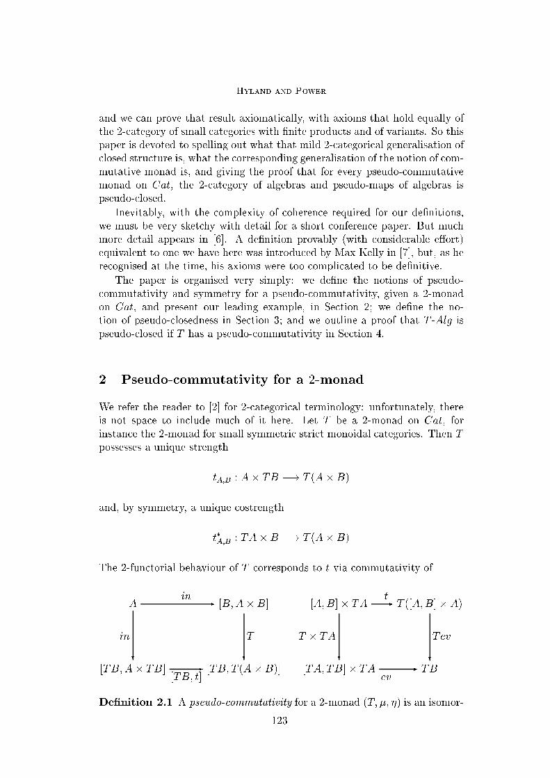
Hyland and Power

and we can prove that result axiomatically, with axioms that hold equally of

the 2-category of small categories with �nite products and of variants. So this

paper is devoted to spelling out what that mild 2-categorical generalisation of

closed structure is, what the corresponding generalisation of the notion of com-

mutative monad is, and giving the proof that for every pseudo-commutative

monad on Cat, the 2-category of algebras and pseudo-maps of algebras is

pseudo-closed.

Inevitably, with the complexity of coherence required for our de�nitions,

we must be very sketchy with detail for a short conference paper. But much

more detail appears in [6]. A de�nition provably (with considerable e�ort)

equivalent to one we have here was introduced by Max Kelly in [7], but, as he

recognised at the time, his axioms were too complicated to be de�nitive.

The paper is organised very simply: we de�ne the notions of pseudo-

commutativity and symmetry for a pseudo-commutativity, given a 2-monad

on Cat, and present our leading example, in Section 2; we de�ne the no-

tion of pseudo-closedness in Section 3; and we outline a proof that T -Alg is

pseudo-closed if T has a pseudo-commutativity in Section 4.

2 Pseudo-commutativity for a 2-monad

We refer the reader to [2] for 2-categorical terminology: unfortunately, there

is not space to include much of it here. Let T be a 2-monad on Cat, for

instance the 2-monad for small symmetric strict monoidal categories. Then T

possesses a unique strength

tA;B : A� TB �! T (A�B)

and, by symmetry, a unique costrength

t�A;B : TA� B �! T (A�B)

The 2-functorial behaviour of T corresponds to t via commutativity of

Ain - [B;A� B] [A;B]� TA

t- T ([A;B]� A)

[TB;A� TB]

in

?

[TB; t]- [TB; T (A� B)]

T

?[TA; TB]� TA

T � TA

?

ev- TB

Tev

?

De�nition 2.1 A pseudo-commutativity for a 2-monad (T; �; �) is an isomor-

123

Hyland and Power

phic modi�cation

TA� TBt�- T (A� TB)

T (t)- T 2(A�B)

+ A;B

T (TA� B)

t

?

T t�- T 2(A� B)

�A�B

- T (A� B)

�A�B

?

such that the following three strength axioms, two � axioms and two � axioms

hold.

(i) A�B;C � (tA;B � TC) = tA;B�C � (A� B;C)

(ii) A;B�C � (TA� tB;C) = A�B;C � (t�

A;B � TC)

(iii) A;B�C � (TA� t�B;C) = t�A�B;C � ( A;B � C)

(iv) A;B � (�A � TB) is an identity modi�cation

(v) A;B � (TA� �B) is an identity modi�cation

(vi) A;B � (�A � TB) is equal to the pasting

T 2A� TBt� - T (TA� TB)

T t�- T 2(A� TB)T 2t- T 3(A�B)

+ T A;B

T (T 2A�B)

t

?T 2(TA�B)

T t

?

T 2t�- T 3(A�B)

T�A�B

- T 2(A�B)

T�A�B

?

+ TA;B

T 2(TA�B)

T t�

?

�TA�B

- T (TA� B)

�TA�B

?

T t�- T 2(A�B)

�T (A�B)

?

�A�B

- T (A� B)

�A�B

?

(vii) the dual of the above � axiom

There is a little redundancy here, as follows.

Proposition 2.2 Any two of the strength axioms implies the third.

If the modi�cation were an identity, T would be a commutative 2-monad

[7,8] and the axioms would all be redundant. But in our leading example,

where T is the 2-monad on Cat for symmetric strict monoidal categories,

is not an identity but rather is determined by a non-trivial symmetry. We

shall soon spell out that example in detail, but �rst we introduce a further

symmetry condition on a pseudo-commutativity: we do not use this condition

for our main results, but it simpli�es analysis of the examples and we believe

124

Hyland and Power

it will be useful in practice, for example in relation to Bunched Implication

[11], as we shall explain below.

De�nition 2.3 A pseudo-commutativity is symmetric when TcA;B � A;B �

cTB;TA is the inverse of B;A.

The simpli�cation that this de�nition allows is given by the following

proposition.

Proposition 2.4 An isomorphic modi�cation as above is a symmetric pseudo-

commutativity if the symmetry axiom, one strength axiom, one � axiom, and

one � axiom hold.

Finally, we spell out our leading example in detail. Most of the other

examples, which we list afterwards, work similarly.

Example 2.5 Let T be the 2-monad for symmetric strict monoidal categories.

� Given a category A, the category TA has as objects sequences

a1 : : : an

of objects of A (with maps generated by symmetries and the maps of A);

the tensor product is concatenation.

� Given two categories A and B, the category TA� TB has as objects pairs

((a1 : : : an); (b1 : : : bm))

and the two maps TA�TB �! T (A�B) take such pairs to the sequences

of all (ai; bj) ordered according to the two possible lexicographic orderings.

In fact

TA� TBt�- T (TA� B)

T (t)- T 2(A�B)�A�B- T (A� B)

gives the ordering

(a1; b1); (a1; b2); : : :

in which the �rst coordinate takes precedence, while

TA� TBt- T (TA� B)

T (t�)- T 2(A�B)�A�B- T (A� B)

gives the ordering

(a1; b1); (a2; b1); : : :

in which the second coordinate takes precedence.

� The component A;B of the modi�cation is given by the unique symmetry

mediating between the two lexicographic orders.

125

Hyland and Power

We now indicate the force of our various axioms as they appear here.

� The strength axioms concern the various lexicographic orderings of the se-

quences (ai; bj; ck) where again there is just one ai (or bj or ck). Various

orderings are identi�ed and as a result there are in each case prima facie

two processes for mediating between the orderings: these are equal. So the

axioms re ect the fact that there is a unique way to mediate between a pair

of orderings.

� The � axioms express the fact that the two lexicographic orderings of the

(ai; bj) are equal if one of n or m is 1.

� The � axioms take more explaining. Take a sequence a1; : : : ; an of se-

quences ai1; : : : aim(i). Concatenation gives a sequence aij where the order

is determined by the precedence (i; j): that is, i takes precedence over j.

Take this concatenated sequence together with a sequence b1; : : : ; bp. Then

A;B � (�A � TB) mediates between the order on the (aij; bk) with prece-

dence (i; j; k) and that with precedence (k; i; j). However we can also use

� � T A;B � t� to mediate between the orders determined by (i; j; k) and

(i; k; j), and use � � T t� � TA;B to mediate between the orders determined

by (i; k; j) and (k; i; j). Composing these two gives the �rst. So again the

axioms re ect the fact that there is a unique way to mediate between a pair

of orderings.

� The symmetry axiom just says that if you swap the order twice, you return

to where you began.

Further examples of symmetric pseudo-commutative monads, for which we

shall not spell out the details, are given by those for

(i) Symmetric monoidal categories.

(ii) Categories with strictly associative �nite products. (Categories with

strictly associative �nite coproducts.)

(iii) Categories with �nite products. (Categories with �nite coproducts.)

(iv) Categories with an action of a symmetric strictly associative monoidal

category.

(v) Symmetric strict monoidal categories with a strict monoidal endofunctor.

(vi) Symmetric monoidal categories with a strong monoidal endofunctor.

These examples are used widely for modelling contexts, or parallelism, or

interaction in computer science [1,4,5,9], and one can build combinations as

used in [11] or variants. In more detail, �nite products are used extensively

for modelling contexts, for instance in [4]. A subtle combination of �nite

products and symmetric monoidal structure is used to model parallelism in

[9]. And symmetric monoidal structure is used to model interaction in [1].

And in current research, Plotkin is using a category with an action of a sym-

metric monoidal category to model call-by-name and call-by-value, along the

lines of symmetric premonoidal categories being represented as the action of

126

Hyland and Power

a symmetric monoidal category on a category [12]. For a non-example of the

symmetry condition, we believe that there is a natural pseudo-commutativity

on the 2-monad for braided monoidal categories which is not symmetric.

We can prove that our de�nition of symmetric pseudo-commutativity im-

plies that adumbrated by Kelly in [7], which tells us

Theorem 2.6 If T is a symmetric pseudo-commutative monad on Cat, then

T lifts to a 2-monad on the 2-category SymMon of small symmetric monoidal

categories and strong symmetric monoidal functors.

This result seems likely to relate to Bunched Implication [11], where the

underlying �rst order structure involves a symmetric monoidal category, so

an object of SymMon, that possesses �nite products, so has T -structure for

the symmetric pseudo-commutative monad for small categories with �nite

products. We do not immediately have a more direct relationship with linear

logic, as the latter involves a comonad !, and the 2-category of small categories

equipped with a comonad is not an example of the 2-category of algebras for

a pseudo-commutative 2-monad.

3 Pseudo-closed 2-categories

In this section, we de�ne the notion of a pseudo-closed 2-category.

De�nition 3.1 A pseudo-closed 2-category consists of a 2-category K, a 2-

functor

[�;�] : Kop �K �! K

and a 2-functor V : K �! Cat, together with an object I of K and transfor-

mations j, e, i, k, with components

� jA : I �! [A;A] pseudo-dinatural in A,

� eA : [I; A] �! A natural in A, and iA : A �! [I; A] pseudo-natural in A,

� kA;B;C : [B;C] �! [[A;B]; [A;C]] natural in B and C and dinatural in A,

such that V [�;�] = K(�;�) : Kop � K �! Cat, e and i form a retract

equivalence, and

(i)

IjB - [B;B]

@@@@@

j[A;B]R

[[A;B]; [A;B]]

kA

?

127

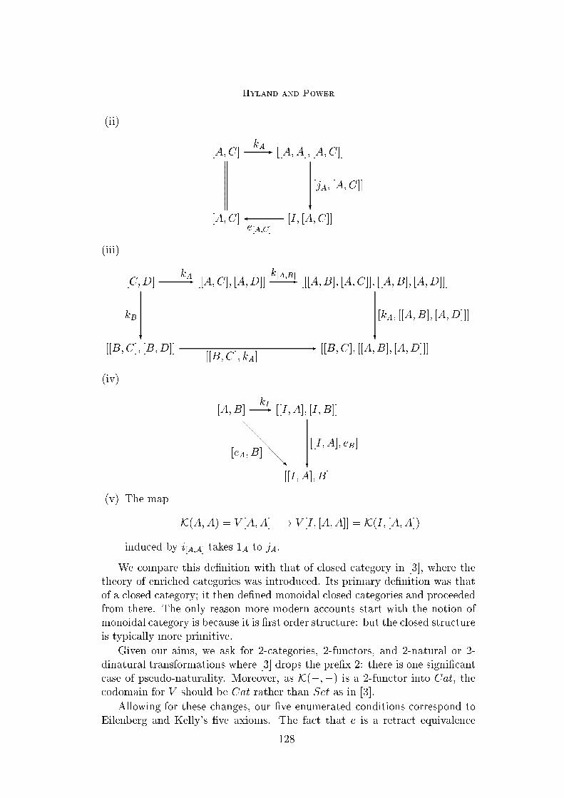
Hyland and Power

(ii)

[A;C]kA- [[A;A]; [A;C]]

[A;C]

wwwwwwwww

�e[A;C]

[I; [A;C]]

[jA; [A;C]]

?

(iii)

[C;D]kA- [[A;C]; [A;D]]

k[A;B]- [[[A;B]; [A;C]]; [[A;B]; [A;D]]]

[[B;C]; [B;D]]

kB

?

[[B;C]; kA]- [[B;C]; [[A;B]; [A;D]]]

[kA; [[A;B]; [A;D]]]

?

(iv)

[A;B]kI- [[I; A]; [I; B]]

@@@@@

[eA; B]R

[[I; A]; B]

[[I; A]; eB]

?

(v) The map

K(A;A) = V [A;A] �! V [I; [A;A]] = K(I; [A;A])

induced by i[A;A] takes 1A to jA.

We compare this de�nition with that of closed category in [3], where the

theory of enriched categories was introduced. Its primary de�nition was that

of a closed category; it then de�ned monoidal closed categories and proceeded

from there. The only reason more modern accounts start with the notion of

monoidal category is because it is �rst order structure: but the closed structure

is typically more primitive.

Given our aims, we ask for 2-categories, 2-functors, and 2-natural or 2-

dinatural transformations where [3] drops the pre�x 2: there is one signi�cant

case of pseudo-naturality. Moreover, as K(�;�) is a 2-functor into Cat, the

codomain for V should be Cat rather than Set as in [3].

Allowing for these changes, our �ve enumerated conditions correspond to

Eilenberg and Kelly's �ve axioms. The fact that e is a retract equivalence

128

Hyland and Power

rather than an isomorphism as in [3] is signi�cant. We have no choice if

we are to include our leading example: one might hope that the 2-category

of small symmetric monoidal categories would have invertible e, but it does

not; and because e is not an isomorphism, we do not have the Eilenberg and

Kelly versions of conditions 2 and 4 which are expressed in terms of i; and

those conditions would fail in our leading example. Moreover i is only pseudo-

natural in examples. We note that we are able to give our restricted de�nition

so that T -Alg will be an example where all the structure maps other than iAare strict maps of T -algebras.

This is not the most general possible notion of pseudo-closedness. Even

Eilenberg and Kelly could have asked for an isomorphism between V [�;�]

and K(�;�): their choice of equality means that a monoidal category subject

to the usual adjointness condition need not be closed in their sense. But our

examples allow us considerable strictness, so we take advantage of that to

provide a relatively simple de�nition.

On the other hand, it does not contain all axioms that hold of our class

of examples either. In particular, our pseudo-natural transformation i and

our pseudo-dinatural transformation j satisfy strictness conditions along the

lines that, for some speci�c classes of maps, the isomorphism given by pseudo-

naturality is in fact an identity. However, at present, we have no theorems that

make use of such facts, and adding them to the de�nition would complicate

rather than simplify it, so we have not introduced them as axioms.

4 Pseudo-closed structure on T -Alg

We consider the 2-category T -Alg of strict T -algebras and pseudo-maps of

T -algebras as developed in [2], for a 2-monad T on Cat. We can readily

generalise beyond Cat, but this contains the examples of primary interest to

us: the 2-category of small symmetric monoidal categories and strong sym-

metric monoidal functors is an example, as is the category of small categories

with �nite products and �nite product preserving functors, etcetera. We write

A = (A; a) for a typical T -algebra. A pseudo-map (f; �f) : A �! B is given

by data

TATf - TB

+ �f

A

a

?

f- B

b

?

where the isomorphic 2-cell �f satis�es � and � conditions. We often write f =

(f; �f) : A �! B for such a pseudo-map, the 2-cell usually being understood.

Given a pseudo-commutativity for T , we show that for any T -algebras A

129

Hyland and Power

and B, the category T -Alg(A;B) has a T -algebra structure de�ned pointwise,

i.e., it inherits a T -algebra structure from the cotensor, i.e., from the functor

category [A;B] with pointwise T -structure.

In order to express the de�nition, we recall two sorts of limits in 2-categories.

Given a pair of parallel 2-cells f; g : X �! Y in a 2-category K, the iso-

inserter of f and g consists of the universal 1-cell i : I �! X and isomorphic

2-cell : fi ) gi, universally inserting an isomorphism between f and g.

Given parallel 2-cells �; � : f ) g : X �! Y , the equi�er of � and � is the

universal 1-cell e : E �! X making �e = �e.

Proposition 4.1 [2] For any 2-monad T on Cat, the 2-category T -Alg has

and the forgetful 2-functor U : T -Alg �! Cat preserves iso-inserters and

equi�ers.

It is routine to describe iso-inserters and equi�ers in Cat by considering

their universal properties as they apply to functors with domain 1. With these

de�nitions, we can de�ne the pseudo-closed structure of T -Alg for pseudo-

commutative T .

De�nition 4.2 Given T -algebras A = (A; a) and B = (B; b), we construct a

new T -algebra in three steps.

(i) Take the iso-inserter (i : In �! [A;B]; �0) of

[A;B]�A;B-

[a;B]- [TA;B]

where the underlying 1-cell of �A;B is de�ned by the composite

[A;B]T- [TA; TB]

[TA; b]- [TA;B]

which canonically but not obviously lifts to a map in T -Alg, with 2-cell

structure de�ned by use of , So we get a universal 2-cell �0 : �A;B � i �!

[a;B] � i.

(ii) Take the equi�er e0 : Eq0 �! In of [�A;B] � �0 with the identity.

(iii) Take the equi�er e : Eq �! Eq0 of [�A; B] � �0 � e0 with the following

130

Hyland and Power

pasting:

[A;B]�- [TA;B]

�����

i�

+ �0

�����

[a; B]

� @@@@@

�

R

Eq0e0 - In

i - [A;B] [T 2A;B]

@@@@@

iR

+ �0

@@@@@

�

R �����

[Ta;B]

�

[A;B][a; B]- [TA;B]

Here the �nal square commutes by naturality of �, and the domains of

the 2-cells match easily; for the codomains, one must work a little.

We write the resulting T -algebra [A;B] and call it, equipped with the com-

posite

p = i � e0 � e : [A;B] �! [A;B]

and the isomorphic 2-cell

� = �0 � e0 � e : �A;B � p �! [a;B] � p

the exponential A to B.

Taking the canonical constructions of iso-inserters and equi�ers in Cat, it

transpires that our �nal Eq is exactly the category of pseudo-maps from A

to B. So the forgetful 2-functor takes [A;B] to T -Alg(A;B). Moreover the

following universal property follows directly from the construction.

Proposition 4.3 Given T -algebras A = (A; a) and B = (B; b), the T -algebra

[A;B] equipped with

p : [A;B] �! [A;B] and an isomorphic 2-cell � : �A;B � p �! [a;B] � p

satis�es the universal property that for each D, composition with p induces an

isomorphism between T -Alg(D; [A;B]) and the category of cones given by data

f : D �! [A;B] and an isomorphic 2-cell � : �A;B � f �! [a;B] � f

satisfying two equi�cation conditions: one for �, the other for �.

To complete the proof of our main theorem, a delicate notion of multi-

linear map of T -algebras seems of fundamental importance [6]. But the above

is the central point, and, taking the unit to be T1, the free T -algebra on 1,

we have

131

Hyland and Power

Theorem 4.4 If T is a pseudo-commutative 2-monad on Cat, then T -Alg is

a pseudo-closed 2-category.

References

[1] Abramsky, S., Retracing some paths in process algebra, \Proc. CONCUR 96,"

Lect. Notes in Computer Science 1119 (1996) 1{17.

[2] Blackwell, R., G.M. Kelly, and A.J. Power, Two-dimensional monad theory, J.

Pure Appl. Algebra 59 (1989) 1{41.

[3] Eilenberg, S., and G.M. Kelly, Closed categories, \Proc. Conference on

Categorical Algebra (La Jolla 1965)," Springer-Verlag (1966).

[4] Fiore, M., and G.D. Plotkin, An axiomatisation of computationally adequate

domain-theoretic models of FPC, Proc. LICS 94 (1994) 92{102.

[5] Fiore, M., G.D. Plotkin, and A.J. Power, Cuboidal sets in axiomatic domain

theory, Proc. LICS 97 (1997) 268{279.

[6] Hyland, M., and A.J. Power, Pseudo-commutative monads and pseudo-closed

2-categories, J. Pure Appl. Algebra (to appear).

[7] Kelly, G.M., Coherence theorems for lax algebras and for distributive laws,

Lecture Notes in Mathematics 420, Springer-Verlag (1974) 281{375.

[8] Kock, A., Closed categories generated by commutative monads, J. Austral. Math

Soc. 12 (1971) 405-424.

[9] Milner, R., Calculi for interaction, Acta Informatica 33 (1996) 707{737.

[10] Moggi, E., Notions of computation and monads, Information and Computation

93 (1991) 55{92.

[11] O'Hearn, P.W., and D.J. Pym, The logic of bunched implications, Bull. Symbolic

Logic (to appear)

[12] Power, A.J., and E. P. Robinson, Premonoidal categories and notions of

computation, Math. Struct. in Comp. Science 7 (1997) 453{468.

132

MFPS 17 Preliminary Version

Stably Compact Spaces and Closed Relations

Achim Jung

School of Computer Science

The University of Birmingham

Birmingham, B15 2TT

England

Mathias Kegelmann

Fachbereich Mathematik

Technische Universit�at Darmstadt

Schlo�gartenstra�e 7

64289 Darmstadt

Germany

M. Andrew Moshier

Computer Science Department

Chapman University

333 N. Glassell Street

Orange, CA 92666

USA

Abstract

Stably compact spaces are a natural generalization of compact Hausdor� spaces in

the T0 setting. They have been studied intensively by a number of researchers and

from a variety of standpoints.

In this paper we let the morphisms between stably compact spaces be certain

\closed relations" and study the resulting categorical properties. Apart from ex-

tending ordinary continuous maps, these morphisms have a number of pleasing

properties, the most prominent, perhaps, being that they correspond to preframe

homomorphisms on the localic side. We exploit this Stone-type duality to establish

that the category of stably compact spaces and closed relations has bilimits.

1 Introduction

The research reported in this paper derives its motivation from two sources.

For some time, we have tried to extend Samson Abramsky's Domain Theory

This is a preliminary version. The �nal version will be published inElectronic Notes in Theoretical Computer Science

URL: www.elsevier.nl/locate/entcs

Jung, Kegelmann and Moshier

in Logical Form to continuous domains, [1,15,14,17]. This has led to a number

of insights, the most important perhaps being that in order to perform domain

constructions strictly logically, one can invoke a version of Gentzen's cut elim-

ination theorem. This, however, requires that we consider a purer logic than

Abramsky did. Semantically, it then turns out that the notion of morphisms

so captured consists of certain relations, rather than functions, [14, Proposi-

tion 6.5]. This is quite in line with developments in denotational semantics,

where the need for (or the advantages of) relations has been noticed for some

time, [5,3].

Our second motivation stems from the desire to circumvent some of the

diÆculties connected to classical domain theory. As is well known, in order

to get a cartesian closed category of continuous domains, one has to restrict

to a subcategory of FS-domains, [13,1]. Unlike general continuous domains,

a straightforward characterisation of FS-domains via their Stone dual, for

example, is not known. Perhaps as a result of the relative weakness of ourtools for FS-domains, certain basic questions about them remain unresolved.We still do not know whether they coincide with retracts of bi�nite domains

or whether the probabilistic powerdomain can be restricted to this category,[16].

The semantic spaces which we put forward in this paper, in contrast toFS-domains, are very well behaved and understood. They are the so-called

stably-compact spaces. Many equivalent characterisations are known and manyproperties have been discovered for them. Also, they do encompass most cate-gories of continuous domains which have played a role in denotational seman-

tics. As is clear from what we have said at the beginning, we are interestedin the category SCS� of stably compact spaces with closed relations as mor-

phisms. Although a similar set-up has been considered some time ago, [26,Prop. 11.2.5], the explicit relational presentation appears to be new.

The purpose of this paper is to examine the suitability of SCS� as a se-mantic universe. To this end we look at �nitary closure properties and thebilimit construction. The latter, to our great satisfaction, behaves in a very

natural and intuitive way. Speci�cally, we show that the bilimit coincides with

a classical topological limit although it is constructed order-theoretically.

2 The category of of stably compact spaces and closed

relations

2.1 The spaces

We assume standard domain theoretic notation as it is used in [8,1], for exam-

ple. Slightly less well known, perhaps, are the following notions and results.

If X is a topological space and A an arbitrary subset of X then the saturation

of A is de�ned as the intersection of all neighborhoods of A. For any T0-

topological space X, the specialization order of X is the relation vX given by

134

Jung, Kegelmann and Moshier

x vX y if every neighborhood of x is also a neighborhood of y. The saturation

of a subset A can then also be described as the upward closure with respect

to vX . Open set are always upper, that is, saturated. An important fact is

that the saturation of a compact set is again compact, for a set A has exactly

the same open covers as its saturation.

For any topological space X the set of open subsets forms a complete

lattice (X) with respect to subset inclusion. Vice versa, for every complete

lattice L the set of completely prime �lters, denoted pt(L), carries the topology

fOa j a 2 Lg where F 2 Oa if a 2 F . A space is T0 if the assignment, which

associates with a point x 2 X the open neighborhood �lter N(x), is injective.

A space is called sober if the assignment is bijective. See [1, Section 7] for a

detailed introduction to this topic. We are now ready to de�ne the objects of

interest in this paper:

De�nition 2.1 A topological space is called stably compact if it is sober,

compact, locally compact and �nite intersections of compact saturated subsetsare again compact.

Stably compact spaces have been studied intensively (and under manydi�erent names), [8,10,9,24,19,15] but, unfortunately, apart from [17] there

is no single comprehensive reference for their many properties. We thereforestate the main facts needed in the sequel. Our principal technical tool is theHofmann-Mislove Theorem, [11,18]:

Theorem 2.2 Let X be a sober space. There is an order-reversing bijection

between the set K(X) of compact saturated subsets of X (ordered by reversed

inclusion) and Scott-open �lters in (X) (ordered by inclusion). It assigns to

a compact saturated set the �lter of open neighborhoods and to a Scott-open

�lter of open sets their intersection.

One consequence of this which we will need later is that every Scott-open

�lter in (X) is equal to the intersection of all completely prime �lters con-

taining it. Another is the fact that the set K(X) is a dcpo when equipped

with reversed inclusion. For stably compact spaces even more is true:

Proposition 2.3 Let X be a stably compact space.

(i) K(X) is a complete lattice in which suprema are calculated as intersec-

tions and �nite in�ma as unions.

(ii) (X) and K(X) are stably continuous frames.

(iii) In (X) we have O � O0 if and only if there is K 2 K(X) with O �

K � O0.

(iv) In K(X) we have K � K 0 if and only if there is O2(X) with K 0 �

O � K.

As in [15] we use stably continuous frame to denote continuous distributive

lattices in which the way-below relation is multiplicative, that is, in which

135

Jung, Kegelmann and Moshier

x � y; z implies x � y ^ z and in which 1 � 1. They are precisely the

Stone duals of stably compact spaces, see [10, Theorem 1.5]. Note that the

proposition tells us that the complements of compact saturated sets form

another topology on X, called the co-compact topology for X and denoted by

X�. Original and co-compact topology are closely related:

Proposition 2.4 Let X be a stably compact space.

(i) The open sets of X� are the complements of compact saturated sets in X.

(ii) The open sets of X are the complements of compact saturated sets in X�.

(iii) X� is stably compact and (X�)� is identical to X.

(iv) The specialization order of X is the inverse of the specialization order

of X�.

For a stably compact space X, the patch topology of X is the commonre�nement of the original topology and the co-compact topology. It is denotedbyX�. It is the key to making the connection to much earlier work by Leopoldo

Nachbin, [21]: A partially ordered space or pospace is a topological space Xwith a partial order relation vX such that the graph of vX is a closed subset

of X�X. Such a space must be Hausdor� because the diagonal relation, i.e.,the intersection of vX and the opposite partial order wX , is closed.

Theorem 2.5 For a stably compact space X the specialization order together

with the patch topology makes X� into a compact ordered space. Conversely,

for a compact ordered space (X;v) the open upper sets "U = U 2 (X)

form the topology for a stably compact space X", and the two operations are

mutually inverse.

Moreover, for a stably compact space X the upper closed sets of X� are

precisely the compact saturated sets of X.

Notice that for a compact Hausdor� space X, the diagonal relation �X

is a closed (trivial) partial order. By applying Theorem 2.5 to the pospace

(X;�X), we see that the upper opens and lower opens are just the opens ofthe original topology. So X = X� = X�. The converse also holds.

Corollary 2.6 A space X is compact Hausdor� if and only if it is a stably

compact space for which X = X�.

Proof. The patch topology for any stably compact space is Hausdor�. In

the case of a stably compact space for which X = X�, the patch topology is

simply the original. 2

We can thus think of stably compact spaces as the T0 generalization of

compact Hausdor� spaces. The fact that X 6= X� in general forces us to treadcarefully in Section 2.2 as we generalize from closed relations between compact

Hausdor� spaces to closed relations between stably compact spaces.

The importance of stably compact spaces for domain theory is that almost

all categories used in semantics are particular categories of stably compact

136

Jung, Kegelmann and Moshier

spaces.

Proposition 2.7 FS domains, and hence in particular Scott domains and

continuous lattices, equipped with their Scott topologies, are stably compact

spaces.

2.2 The morphisms

The obvious category of stably compact spaces is that of continuous functions,

i.e. the full subcategory SCS of the category of topological spaces Top. The

category that we are really interested in, however, is one that generalizes

KHaus�, the category of compact Hausdor� spaces and closed relations. We

quote the basic de�nitions and results from [14].

The specialization order of a stably compact spaceX is generally not closed

in X � X. Indeed, were it closed, X would be a pospace, hence would beHausdor�. Thus, specialization would be trivial. Specialization, on the otherhand, is reversed by taking the co-compact topology (again, in the Hausdor�

case X = X� so the \reversal" is trivial). Thus:

Proposition 2.8 The specialization order of a stably compact space X is

closed in X �X�.

Proof. Suppose that x 6vX y. Then there is an open set U containing x and

not y. By local compactness, we can assume that U is contained in a compactsaturated neighborhood K of x that also does not contain y. U is an upperset containing x. The complement of K is a lower set containing y. Thus

U � (X nK) is a neighborhood of hx; yi in X �X� that does not meet vX .2

For stably compact spaces X and Y , we call a closed subset R � X �Y� aclosed relation from X to Y and we write it as R : X +- Y . If we spell out

this condition then it means that for x 2 X and y 2 Y such that x 6R y we �nd

an open neighborhood U of x and a compact saturated set K � Y that doesn'tcontain y such that U � (Y nK) \ R = ;. [cf. the proof Proposition 2.8.]Note that every closed relation R satis�es the rule x0 vX x R y vY y

0 =)

x0 R y0.

The composition of closed relations is the usual relation product, R ; S =�hx; zi j (9y) x R y and y S zg. Note that, following usual practice, we write

the composition of relations from left to right, whereas for functions it is from

right to left. To avoid ambiguity we use \;" to indicate left-to-right composi-tion. Notice that the specialization order of any stably compact space X acts

as identity under taking the relation product with closed relations from or to

X and also that the composition of two closed relations is again closed. We

call the category of stably compact spaces with closed relations SCS�.

The Hausdor� case is worth considering separately as it helps to illuminate

the de�nition of closed relations. As we have noted, a stably compact space is

Hausdor� if and only if its topology agrees with its co-compact topology. Thus

137

Jung, Kegelmann and Moshier

our closed relations from X to Y are simply closed subsets of X�Y = X�Y�whenever Y is Hausdor�. Thus SCS� correctly generalizes KHaus�, in which

we could take the morphisms simply as closed subsets of X � Y . The fact

that we could get away with this apparently simpler notion of morphism in

the Hausdor� setting is due essentially to the fact that in compact Hausdor�

spaces the co-compact topology is \hidden from view." In particular, KHaus�

is a full subcategory of SCS� (as well as being a subcategory of Rel).

Note that the obvious forgetful \functor" from SCS� to Rel, the category

of sets with relations, preserves composition but not identities. The only

stably compact spaces for which identity is preserved are those with trivial

specialization orders, i.e., the compact Hausdor� spaces.

Relations between sets can be understood as multi-functions. As the fol-

lowing proposition shows this carries over to our topological setting in an

interesting way.

Proposition 2.9 Let X and Y be stably compact spaces and R : X +- Y a

closed relation then

fR(x) := fy 2 Y j x R yg

de�nes a continuous function from X to K(Y ), where the latter is equipped

with the Scott topology. Conversely, if f : X ! K(Y ) is continuous then

�hx; yi 2 X � Y

�� y 2 f(x)

is a closed relation from X to Y . Moreover, these two translations are mutually

inverse.

To extend this correspondence to the composition of relations and multi-

functions, respectively, we �rst have to de�ne a law of composition on thelatter. To this end recall that K(X) with its Scott topology is again a stablycompact space by Propositions 2.3 and 2.7. Hence we can make K into an

endofunctor on SCS by mapping a continuous function f : X ! Y to the

function K(f) : K(X)! K(Y ) that takes a compact saturated subset K � X

to "f [K]. This endofunctor is part of a monad whose unit takes the saturation

of points and whose multiplication is simply union [22]. Consequently, thecanonical composition of multi-functions is Kleisli composition which turns

out to be the analogue of ordinary relation product.

Proposition 2.10 The category of closed relations SCS� is isomorphic to the

Kleisli category SCSK.

It is generally the case that a category C with a monad T is embedded in

the Kleisli category CT simply by post-composing with the unit of the monad.Moreover, if the units of the monad are monic, then the embedding is faithful.

Hence, SCS is a subcategory of SCSK and thus also of SCS�. Concretely,

138

Jung, Kegelmann and Moshier

this embedding works by taking the hypergraph of a function. The following

proposition characterizes those relations that are really embedded functions:

Proposition 2.11 If f : X ! Y is a continuous function then the hypergraph

�hx; yi 2 X � Y

�� f(x) v y

is a closed relation from X to Y . Conversely, if R : X +- Y is a closed

relation such that for all x 2 X the set fR(x) has a least element r(x) then

r : X ! Y is a continuous function, and this operation is the inverse of the

previous.

Again, the Hausdor� case may help to illuminate this. If f : X ! Y is a

continuous function with Y a compact Hausdor� space, then the hypergraph

is simply the graph of f . This is a closed relation just as classical topology

tells us it should be. Conversely, suppose that a closed relation from X to Yis the graph of a function g. Then clearly fR(x) has a least element g(x) for

each x. Thus g is a continuous function.

2.3 The category

The left adjoint from SCS to the Kleisli category SCSK �= SCS� preservescoproducts. Hence, they are given in SCS� simply as topological coproducts,

i.e., as disjoint unions.

In the category Rel of sets and relations for every relation R : X +- Y

there is the reciprocal relation R� that is given by y R� x () x R y. This isthe main ingredient that makes Rel into an allegory [7]. Our category SCS� fails

to be an allegory exactly because, as we shall see, it lacks a true reciprocationoperation. On the other hand, if R : X +- Y is a closed relation betweenstably compact spaces then R� : Y� +- X� is a closed relation between the

co-compact topologies, and (�)� is an involution on SCS�. The problem is that

it doesn't �x objects. We can think of X� as an upside-down version of X

since the specialization order vX�for the co-compact topology is simply wX ,

i.e. the dual of the one for the original space.

Nonetheless, the maps X 7! X� and R 7! R� comprise a contravariant

functor, showing that SCS� is a self-dual category. Consequently, categoricalproducts (denoted here by X �� Y to avoid con ict with topological products

X � Y ) are also given by disjoint union:

X �� Y �= (X� + Y�)� = (X�

:

[ Y�)� = (X�)�:

[ (Y�)� = X:

[ Y = X + Y:

If a self-dual category is cartesian closed then all objects are isomorphic and

hence the category is equivalent to the category with only one (identity) mor-

phism. This shows that SCS� cannot be cartesian closed.

Since categorical products in SCS� are the same as co-products, let us

look at cartesian products. In SCS they are the categorical product and we

139

Jung, Kegelmann and Moshier

can lift them to SCS� to make SCS� into a symmetric monoidal category.

The tensor product takes the cartesian product of the spaces with the prod-

uct topology and we also embed the morphisms needed for the symmetric

monoidal structure from SCS as described in Proposition 2.11. The de�ni-

tion of the tensor product of two closed relations R and S is pointwise, i,e,

hx; yi R S hx0; y0i : () x R y and x0 R y0. This de�nes a closed rela-

tion and extends to products of continuous functions; for the details see [17,

Section 3.2.4].

With respect to , the category SCS� is closed: Because of (X � Y )� =

X��Y� we see that closed subsets of (X�Y )�Z� are the same thing as closed

subsets of X � (Y� � Z)� which proves SCS�(X Y; Z) �= SCS�(X; Y� Z).

This internal homset Y� Z, however, does not correspond to the \real"

homset SCS�(Y; Z).

The homset SCS�(Y; Z) consists of the closed subsets of Y � Z� which byTheorem 2.5 are precisely the compact saturated subsets of the dual (Y �Z�)�.Hence, we can write the relation space as [Y ) Z] := K(Y� � Z). With this

de�nition and Proposition 2.10 we get

SCS�(X Y; Z) �= SCS�(X; Y� Z) �= SCS�X;K(Y� Z)

�= SCS

�X; [Y ) Z]

�:

So, we see that (�Y ) and [Y ) �] are almost adjoint. The problem is thatthe induced morphism X +- [Y ) Z] is not uniquely determined.

The canonical evaluation morphism is a functional closed relation and forthe induced morphism we can always choose a functional one, and as such it is

unique, i.e. these morphisms come from SCS rather than SCS�. In [23] such asituation is called a Kleisli exponential. There is an alternative description ofthe relation space by observing SCS�(Y; Z) �= SCS

�Y;K(Z)

�: Thus the normal

function space [Y ! K(Z)] with the compact-open topology, which is simplythe Scott topology, yields a space that is homeomorphic to [Y ) Z]. Thisconstruction was �rst studied in [25], although it seems that some of subtleties

concerning the fact that this is only a Kleisli exponential were overlooked.

3 Stone Duality

Next we develop the Stone duality of closed relations. The morphisms between

open set lattices corresponding to closed relations turn out to be preframe

homomorphisms, [2], preserving �nite meets and directed suprema. They

have been studied in a similar framework before, see [26, Prop. 11.2.5], butthe duality with relations seems to be new.

3.1 Relational preimage

If R : X +- Y is a relation and A � X a subset, then we write

[A]R :=�y 2 Y

�� (9x 2 A) x R y

140

Jung, Kegelmann and Moshier

for the usual forward image. The de�nition of the preimage of a subset B � Y

under the relation R is a bit more tricky as there are several candidates. Here,

we are only interested in the universal preimage given by

(8R)[B] :=�x 2 X

�� (8y 2 Y ) x R y =) y 2 B:

This de�nition is useful because 8R turns out to be the right adjoint to [�]R:

Lemma 3.1 If R � X � Y is a relation and A and B are subsets of X and

Y , respectively, then we have

[A]R � B () A � (8R)[B]:

In the usual functional setting the situation is analogous; preimage is right

adjoint to direct image. The connection between relational and functionalpreimage is the following.

Lemma 3.2 If f : X ! Y is a continuous function between stably compact

spaces and F : X +- Y the corresponding closed relation given by the hyper-

graph, then for all upper sets A = "A � Y we have

f�1[A] = (8F )[A]:

We now describe the translation from topological spaces to frames in therelational setting.

Proposition 3.3 If R : X +- Y is a closed relation then 8R is a continuous

semilattice homomorphism from (Y ) to (X), i.e. it preserves �nite in�ma

and directed suprema.

Proof. First, we have to check that for any open V � Y the preimage (8R)[V ]is open. So let x 2 (8R)[V ], or equivalently fR(x) = [x]R � V . We know from

Proposition 2.9 that fR is continuous and thus Proposition 2.3 gives us an open

neighborhood U of x such that fR(x0) � V for all x0 2 U . We conclude x 2

U � (8R)[V ], thus showing that for a closed relation the universal preimage

of an open set is open.

As we have seen in Lemma 3.1, 8R as a function between the full powersets

is a right adjoint. As such it preserves all intersections and thus the �nite meets

in (Y ).

Thus, it is a monotone map and, consequently, to show that it also pre-serves directed suprema we only have to verify (8R)

�S"Vi��S"(8R)[Vi]. So,

we consider an x 2 (8R)�S"

Vi�which means fR(x) �

S"Vi. But as fR(x) is

compact we can �nd an index i such that fR(x) � Vi and, equivalently, such

that x 2 (8R)[Vi]. 2

We call �R the restriction and co-restriction of 8R to the open subsetsof X and Y to simplify notation. Going from a relation to the forward im-

age function is well-known to be functorial, and so is taking adjoints. By

141

Jung, Kegelmann and Moshier

Lemma 3.1 this implies that universal preimage is also functorial. Clearly,

�vX is the identity on �(X) = (X) as all open sets are upper sets. Thus

� is a contravariant functor from SCS� to the category of stably continuous

frames and Scott continuous semilattice homomorphisms which we denote

by SCF�.

Just like we also have to adjust the functor pt to the relational setting.

Consider a homomorphism � : L!M . We de�ne the relation pt�(�) : pt�(M)+- pt�(L) by

Q pt�(�) P :() ��1[Q] � P

where pt� on objects behaves just like the usual pt, i.e., P and Q are com-

pletely prime �lters in L and M , respectively. Alternatively, we can identify

completely prime �lters with their characteristic functions which are frame

morphisms to 2, the two-element lattice. For two such points p : L ! 2 andq : M ! 2 the above de�nition becomes

q pt�(�) p :() q Æ � v p:

Proposition 3.4 If � : L ! M is a continuous semilattice homomorphism,

then pt�(�) : pt�(M) +- pt�(L) is a closed relation.

Proof. Suppose Q � M and P � L are completely prime �lters such that

��1[Q] * P . As � is Scott continuous and Q completely prime and thus, inparticular, Scott open, the set ��1[Q] is also Scott open. Because it is alsonot contained in P and L is a continuous lattice we can �nd an x 2 ��1[Q]nP

such that ��x * P . On the other hand Q, as an upper set, is the union ofprincipal �lters "y for y 2 Q and hence we get ��1[Q] = ��1

�Sf"y j y 2 Qg

�=S�

��1["y]�� y 2 Q 3 x. This means that we can �nd a y 2 Q such that

x 2 ��1["y].

As L is stably continuous, the set ��x is a Scott open �lter which corresponds

to the compact saturated subset�P 2 pt�(L)

����x � P

of pt�(L) by the

Hofmann-Mislove theorem. Now, we consider the open subset of pt�(M) �

pt�(L)� which is given as the product of the open set corresponding to y andto the complement of the compact saturated set corresponding to ��x, and weclaim that this is a neighborhood of hQ;P i that doesn't meet R�. Clearly,

hQ;P i is in this set, and if Q0 2 pt�(M) and P 0 2 pt�(L) are such that y 2 Q0

and ��x * P 0 we get ��1[Q0] � ��1�"y�3 x and thus ��1[Q0] � ��x which

implies ��1[Q0] * P 0. 2

Now we have all the ingredients for a duality between SCS� and SCF�. It

remains to check that the categorical conditions are indeed met.

Theorem 3.5 The contravariant functors � and pt� are part of a dual equiv-

alence between the categories SCF� and SCS�.

Proof. We begin by showing that pt� is indeed a functor. Clearly, pt�(idL) =

vpt�(L), the identity closed relation on pt�(L). The interesting direction for

142

Jung, Kegelmann and Moshier

functoriality is to show that pt�( �) � pt�( ); pt�(�), where � : L!M and

: M ! N are continuous semilattice morphisms. Let P 2 pt�(N) and P 0 2

pt�(L) be such that P (pt�( Æ �)) P 0, or equivalently that ��1� �1[P ]

�� P 0.

We need to �nd a completely prime �lter Q � M that satis�es �1[P ] � Q

and ��1[Q] � P 0. Unfortunately, �1[P ] in general is only a Scott open �lter,

not a point in M .

However, by the Hofmann-Mislove Theorem, 2.2, we have �1[P ] =TfQ 2

pt�(M) j �1[P ] � Qg. So for the sake of contradiction, assume there exists

xQ 2 ��1[Q] n P 0 for all Q � �1[P ]. Then the supremumWxQ of all these

elements does not belong to P 0 because P 0 is completely prime; on the other

hand, �(WxQ) belongs to all Q � �1[P ] by monotonicity of �, hence to

�1[P ]. This contradicts the assumption ��1[ �1[P ]] � P 0.

To show that � and pt� give rise to a duality between SCF� and SCS�

we have to check that their actions on morphisms are mutually inverse. So,suppose R : X +- Y is a closed relation and N(x) and N(y) are the openneighborhood �lters of two points x 2 X and y 2 Y . We get

N(x) (pt�(8R)) N(y) () (8R)�1�N(x)

�� N(y)

()�8V 2 �(Y )

�V 2 (8R)�1

�N(x)

�=) V 2 N(y)

()�8V 2 �(Y )

�x 2 (8R)[V ] =) y 2 V

()�8V 2 �(Y )

�[x]R � V =) y 2 V

Clearly, x R y implies this last condition and the converse follows from thefact that [x]R is saturated.

Finally, we take a continuous semilattice morphism � : L ! M and showthat

��(pt�(�))

��fP 2 pt�(L) j x 2 Pg

�=�Q 2 pt�(M)

�� �(x) 2 Q for any

x 2 L:�8 pt�(�)

���P 2 pt�(L) j x 2 P

�

=nQ 2 pt�(M)

�� �8P 2 pt�(L)�Q (pt�(�)) P =) x 2 P

o

=nQ 2 pt�(M)

�� �8P 2 pt�(L)���1[Q] � P =) x 2 P

o

As before we use the fact that ��1[Q] is a Scott-open �lter and hence by the

Hofmann-Mislove Theorem equal to the intersection of all completely prime

�lters containing it. The expression then re-writes to fQ 2 pt�(M) j x 2

��1[Q]g which is equal to fQ 2 pt�(M) j �(x) 2 Qg as desired. 2

It is interesting to consider the Stone dual of the involution on SCS� that we

discussed in Section 2.3. The co-compact topology on a stably compact space

has precisely the compact saturated subsets of the original space as closed

sets which implies �(X�) = (X�) �= K(X). From the Hofmann-Mislove

Theorem we know that K(X) is in one-to-one correspondence to the Scott

open �lters in (X). The latter can also be understood via their characteristic

functions which are precisely the continuous semilattice homomorphisms to 2,

the two-element lattice. Putting it all together we get (X�) �= K(X) �=

143

Jung, Kegelmann and Moshier

SCF��(X); 2

�and we see that this self-duality in localic terms is exactly the

Lawson duality of stably continuous semilattices [20].

3.2 Functions revisited

We know from Proposition 2.11 that SCS embeds faithfully in SCS� and also

how to recognize the morphisms that arise from this embedding as hypergraphs

of functions. We refer to a closed relation as functional if it is the hypergraph

of a continuous function. Similarly the category SCF� contains a subcategory

of functional arrows.

Proposition 3.6 If R : X +- Y is a functional closed relation then �(R)

preserves �nite (and consequently all) suprema. Conversely, if � : L ! M is

a frame homomorphism then pt�(L) is functional.

Proof. If � is a frame homomorphism then for any completely prime �lterQ � M the preimage ��1[Q] is completely prime. Hence, this is the least

completely prime �lter P � L such that ��1[Q] � P .

For the converse observe that the forward image [x]R of any point x has a

least element and hence will be contained in either U or V i� it is containedin U [ V . This shows that 8R preserves �nite suprema. 2

This result, of course, is very similar to the classical Stone duality be-

tween SCS, the category of stably compact spaces with continuous functions,and SCF�_, stably continuous lattices with frame homomorphisms. There thefunctors and pt act on morphisms as follows: (f) is simply the preim-

age function f�1[�] and similarly pt(�) takes a completely prime �lter P tothe completely prime �lter ��1[P ]. As a corollary of the previous proposi-

tion we get that pt� and � commute with the embeddings of the functional

subcategories.

Corollary 3.7 The diagram of functors

SCS -�pt

Frm

SCS�

i

?

\

�

-�pt�

SCF�

j

?

\

commutes in the sense that j Æ = � Æ i and i Æ pt� = pt Æ j.

Proof. The �rst equality was proved in Lemma 3.2. For the second, take a

frame morphism � : L ! M . It is mapped by i Æ pt to the hypergraph of the

preimage function, i.e. the closed relation that relates Q 2 pt(M) = pt�(M)

to P 2 pt(L) = pt�(L) if and only if ��1[Q] � P which is precisely pt�(j(�)).2

144

Jung, Kegelmann and Moshier

As a consequence of this corollary the operation which extracts from a

functional relation the underlying continuous function (which exists by Propo-

sition 2.11) is just the composition pt Æ �. It follows that this is functorial.

We denote it by U .

There is a more categorical way to identify the functional morphisms in the

two dual categories. As we have seen in Section 2.3, the products on the func-

tional subcategory give rise to a symmetric monoidal structure on the larger

relational category. In addition, the diagonals �A : A ! A � A and mor-

phisms !A to the terminal object induce a diagonal structure. The functional

morphisms are then characterized as the total and deterministic morphisms,

i.e. the ones for which ! and �, respectively, are natural transformations. For

more details see [17, Section 3.3].

4 Subspaces

There are a number of di�erent concepts of \good subspace" in Topology as

often simply carrying the induced topology is too weak. One very useful onethat is well-known in domain theory is that of an embedding-projection pair.It combines the categorical notion of section retraction pair with the order

theoretic notion of adjunction. It is then an immediate corollary that thespace that is the codomain of the section carries the subspace topology. In

the following we will generalize this to the relational setting.

4.1 Perfect relations

We start by de�ning a special class of relations that will be important when

we characterize relations that have adjoints.

De�nition 4.1 We say that a closed relation R : X +- Y is perfect if forall compact saturated sets K � Y the preimage (8R)[K] is compact.

Perfect relations can alternatively be characterized in terms of their Stone

duals.

Proposition 4.2 A closed relation R : X +- Y is perfect if and only if

�(R) preserves the way-below relation.

Proof. Let us assume that R is perfect and U � V are open subsets of Y .Then there is a compact saturated set K � Y such that U � K � V and weget �(R)(U) = (8R)[U ] � (8R)[K] � (8R)[V ] = �(R)(V ). By assumption

(8R)[K] is compact and hence we conclude �(R)(U)� �(R)(V ).

Conversely, suppose �(R) preserves way-below and K � Y is compact

saturated. As a saturated set, K it is the intersection of all the open sets thatcontain it and we compute

(8R)[K] = (8R)�\

#fU 2 �(Y ) j K � Ug

�=\

#

�(8R)[U ]

�� K � U

145

Jung, Kegelmann and Moshier

where the last equality follows because, by Lemma 3.1, 8R is a right adjoint

and hence preserves arbitrary intersections in P(Y ). Now we claim that this

last intersection is taken over a �lterbase for a Scott open �lter in �(X) =

(X). The set�(8R)[U ]

�� K � Uis clearly �ltered. To see that it is

generates a Scott open �lter take U 2 (Y ) that contains K. Since Y is

locally compact, the neighborhood �lter of the compact set K has a basis

of compact saturated sets. This means that there is an open set V and a

compact set K 0 such that K � V � K 0 � U . This implies V � U and hence

by assumption (8R)[V ]� (8R)[U ].

By the Hofmann-Mislove Theorem the intersection over a Scott open �l-

ter of open sets, and hence also of a �lterbase for such a �lter, is compact

saturated. This shows that (8R)[K] is compact and �nishes the proof. 2

This extends the classical situation of functions between stably compact

spaces (or, more generally, locally compact sober spaces), [10, Remark 1.3].Since the Stone dual of a function has an upper adjoint, perfectness in that

situation can be further characterized by the adjoint being Scott-continuous(loc. cit.). Because of Corollary 3.7 we have that a continuous function be-tween stably compact spaces is perfect in the classical sense if and only if the

corresponding relation given by the hypergraph is perfect in our sense.

It may be worthwhile to add a few words about terminology here. As we

quoted, perfect maps have (at least) three di�erent characterizations and fur-thermore many useful properties. Depending on what is considered essential

in a given situation, additional assumptions are made in order to preservecertain key properties in the absence of local compactness, sobriety or both.This has led to an abundance of di�erent concepts for which it now appears

impossible to establish a coherent terminology. Either of \proper" [4,10] or\perfect" [12,9,6] is usually used but it is not clear where the boundary be-tween the two ought to be drawn. Our choice of \perfect" follows the more

recent custom of reserving \proper" for slightly stronger requirements even in

the case of locally compact sober spaces.

We also note that perfect functions between stably compact spaces are ex-

actly those which are continuous with respect to both original and co-compact

topology. This implies that they are exactly those maps which are monotone

and patch continuous. To summarize:

Proposition 4.3 Let f : X ! Y be a function between stably compact spaces

and R : X +- Y the corresponding hypergraph. Then the following are equiv-

alent:

(i) R is perfect;

(ii) f is perfect with respect to the original topologies;

(iii) f is perfect with respect to the co-compact topologies;

(iv) f is monotone and patch continuous.

There is yet another approach to perfectness via uniform continuity: For

146

Jung, Kegelmann and Moshier

every stably compact space there is a unique quasi-uniformity U such that U

induces the topology and U�1 induces the co-compact topology. A continuous

function f : X ! Y between stably compact spaces is perfect if and only if it

is uniformly continuous with respect to these unique quasi-uniformities on X

and Y . For details see [25, Theorem 3].

In a way, perfect continuous functions seem to be a better notion of mor-

phisms for the category SCS than just continuous ones, as open and compact

saturated sets play similarly important roles. Moreover, with these morphisms

we can explain in which way the patch topology is a \natural" construction:

Every continuous function between compact Hausdor� spaces is perfect, and

hence this category embeds fully and faithfully into SCS with perfect maps.

Now, taking the patch topology is simply the right adjoint, i.e. the co-re ector,

for this inclusion functor, [6].

Returning to closed relations again, perfectness is linked to openness. Wesay that a closed relation R : X +- Y is open if for all open sets U � X the

forward image [U ]R is open.

For the next proposition we need the following observation which relates

forward image, universal preimage, complementation and reciprocation:

Lemma 4.4 If R : X +- Y is a relation in Rel and M � X is an arbitrary

subset then [X nM ]R = Y n (8R�)[M ].

Proof. For y 2 Y we have

y 2 [X nM ]R () (9x 2 X nM) x R y

() y =2 (8R�)[M ]

() y 2 Y n (8R�)[M ]:

2

Proposition 4.5 A closed relation R : X +- Y is open if and only if the

reciprocal relation R� : Y� +- X� is perfect.

Proof. Let us assume that R is open. We take a compact saturated set

K 2 K(X�) and have to show that (8R�)[K] is compact in Y�. By Theorem 2.5

the condition K 2 K(X�) is equivalent to X nK 2 (X) and the openness of

R means that [X nK]R is open. By the previous lemma we have [X nK]R =Y n (8R�)[K] 2 (Y�) which, again by Theorem 2.5, implies that (8R�)[K] isa compact saturated subset of Y�.

Conversely, if R� is perfect and U 2 (X) then X nU is compact saturatedinX�. From the previous lemmawe get (8R�)[X n U ] = Y n Y n (8R�)[X n U ] =

Y n [X n (X n U)]R = Y n [U ]R which is a compact saturated subset of Y� be-

cause of the perfectness of R�. Consequently, its complement [U ]R is an open

subset of Y . 2

147

Jung, Kegelmann and Moshier

4.2 Adjunctions

As usual in an order-enriched category, we say that for two closed relations

R : X +- Y is the left or lower adjoint of S : Y +- X if S ; R : X +- X

is below the identity and if R ; S : Y +- Y is above the identity on Y .

Likewise, S is called the right or upper adjoint of R. The question is what

is the right order on the homsets SCS�(X; Y ). One choice is subset inclusion

but it turns out to be better to use the one induced from the corresponding

homsets SCS�X;K(Y )

�, in keeping with Proposition 2.10. Since K(Y ) is

ordered by reverse inclusion this means that the relations in the homsets for

SCS� are also ordered by reverse inclusion of their graphs. Note that adjoints

determine each other uniquely as is the case in any order-enriched category.

Lemma 4.6 The functors � and pt� preserve the order on the homsets, thus

making SCS� and SCF� dually equivalent as order-enriched categories. Conse-

quently, we have R a S for closed relations if and only if �(S) a �(R).

Proof. The �rst claim can easily be veri�ed from the de�nition of the twofunctors. Then the second is an immediate consequence. Note, however, that

because of contravariance the role of lower and upper adjoint are reversed. 2

Upper adjoints have a very concise characterization:

Theorem 4.7 A closed relation R : X +- Y has a lower adjoint if and only

if it is perfect and functional.

Proof. From the previous lemma we know that R has a lower adjoint if and

only if �(R) has an upper adjoint. As we know, �(R) is a continuoussemilattice homomorphism and as a monotone function between the completelattices �(Y ) = (Y ) and �(X) = (X) it is a lower adjoint if and only if

it preserves all suprema. By Proposition 3.6 this is the case precisely when R

is functional.

In this case we have an upper adjoint u : �(X)! �(Y ), but it need not

be a continuous semilattice homomorphism. As an upper adjoint it preserves

all in�ma, but it is Scott continuous if and only if its adjoint �(R) preservesthe way-below relation (see [1, Proposition 3.1.14]). From Proposition 4.2 weknow that this is equivalent to R being perfect. 2

Using Proposition 4.3 above we can rephrase this as follows.

Corollary 4.8 A closed relation has a lower adjoint if and only if it is func-

tional and the corresponding function is patch continuous, i.e. continuous with

respect to the patch topologies.

In the case of Hausdor� spaces the last condition is trivially true since the

patch topology is simply the original topology. Hence, we get the following

result.

Corollary 4.9 A closed relation between compact Hausdor� spaces is a con-

tinuous function if and only if it has a lower adjoint in SCS�.

148

Jung, Kegelmann and Moshier

-

Le

e

e

e e� J

JJJ

1

0

b

?

S BU a

Fig. 1. A non-functional embedding retraction pair.

Consider the two posets given in Figure 1. We de�ne two closed relations

L := f0g � B [ f1g � fa; bg and U := f?g � S [ fa; bg � f1g which is the

hypergraph of the function that maps ? to 0 and identi�es a and b by mapping

them to 1. We have L ; U = idS and also U ; L v idB which shows that they

form a embedding-projection pair in the sense that L is a lower adjoint sectionand U the corresponding upper adjoint retraction. This example shows that

embeddings need not be functional.

We can, however, say explicitly what this lower adjoint does. Essentially

it is just taking preimages under the function corresponding to its adjoint:

Proposition 4.10 Let u : X ! Y be a perfect continuous function between

stably compact spaces, U : X +- Y its hypergraph and L the lower adjoint.

Then we have

y L x () x 2 (8U)["y] () y � u(x)

and the corresponding multi-function fL : Y ! K(X) satis�es

fL(y) = u�1["y]:

Proof. Note that we have x 2 (8U)["y] () x 2 u�1["y] by Lemma 3.2,

and hence the descriptions of the adjoint given in the proposition agree.

We begin by showing that L is a closed relation. The easiest proof is to

show that fL is continuous: It factorizes as Y"- K(Y )

u�1[�]- K(X) wherethe �rst function is already known to be continuous. The spaces K(Y ) and

K(X) carry the Scott topology and directed suprema are given by �ltered

intersections which are preserved by the preimage function u�1[�]. So, fL is a

composition of continuous functions.

To show L a U we have to check vX = idX � U ;L and L;U � idY = vY

since the order on the homsets is reversed inclusion. So, for x v x0 we have

x U u(x) L x0 since u(x) v u(x0). For the second inclusion, y L x U y0 impliesy v u(x) v y0.

2

149

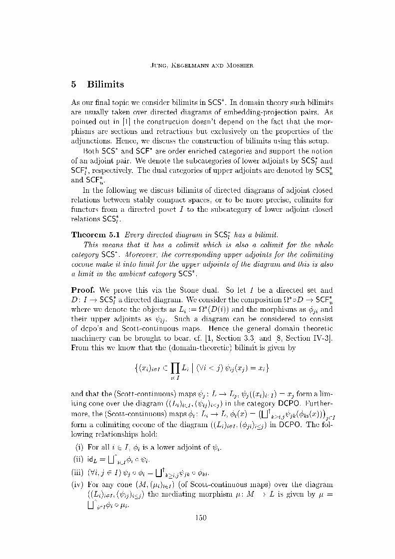
Jung, Kegelmann and Moshier

5 Bilimits

As our �nal topic we consider bilimits in SCS�. In domain theory such bilimits

are usually taken over directed diagrams of embedding-projection pairs. As

pointed out in [1] the construction doesn't depend on the fact that the mor-

phisms are sections and retractions but exclusively on the properties of the

adjunctions. Hence, we discuss the construction of bilimits using this setup.

Both SCS� and SCF� are order enriched categories and support the notion

of an adjoint pair. We denote the subcategories of lower adjoints by SCS�l and

SCF�l , respectively. The dual categories of upper adjoints are denoted by SCS�uand SCF�u.

In the following we discuss bilimits of directed diagrams of adjoint closed

relations between stably compact spaces, or to be more precise, colimits for

functors from a directed poset I to the subcategory of lower adjoint closed

relations SCS�l .

Theorem 5.1 Every directed diagram in SCS�l has a bilimit.

This means that it has a colimit which is also a colimit for the whole

category SCS�. Moreover, the corresponding upper adjoints for the colimiting

cocone make it into limit for the upper adjoints of the diagram and this is also

a limit in the ambient category SCS�.

Proof. We prove this via the Stone dual. So let I be a directed set andD : I ! SCS�l a directed diagram. We consider the composition �ÆD! SCF�uwhere we denote the objects as Li := �(D(i)) and the morphisms as �ji andtheir upper adjoints as ij. Such a diagram can be considered to consistof dcpo's and Scott-continuous maps. Hence the general domain theoretic

machinery can be brought to bear, cf. [1, Section 3.3] and [8, Section IV-3].

From this we know that the (domain-theoretic) bilimit is given by

�(xi)i2I 2

Yi2I

Li

�� (8i < j) ij(xj) = xi

and that the (Scott-continuous) maps j : L! Lj, j((xi)i2I) = xj form a lim-

iting cone over the diagram ((Li)i2I ; ( ij)i�j) in the category DCPO. Further-

more, the (Scott-continuous) maps �i : Li ! L, �i(x) =�F"

k�i;j jk(�ki(x))�j2I

form a colimiting cocone of the diagram ((Li)i2I ; (�ji)i�j) in DCPO. The fol-lowing relationships hold:

(i) For all i 2 I, �i is a lower adjoint of i.

(ii) idL =F"

i2I�i Æ i.

(iii) (8i; j 2 I) j Æ �i =F"

k�i;j jk Æ �ki.

(iv) For any cone (M; (�i)i2I) (of Scott-continuous maps) over the diagram

((Li)i2I ; ( ij)i�j) the mediating morphism � : M ! L is given by � =F"

i2I�i Æ �i.

150

Jung, Kegelmann and Moshier

(v) For any cocone (M; (�i)i2I) (of Scott-continuous maps) over the diagram

((Li)i2I ; (�ji)i�j) the mediating morphism � : L ! M is given by � =F"

i2I�i Æ i.

The objects and morphisms of the category SCF� have additional structure,

so we need to show the following:

(a) L is a complete lattice.

(b) L is continuous.

(c) L is distributive.

(d) The way-below relation on L is multiplicative and 1� 1.

(e) For all i 2 I, �i and i preserve �nite in�ma.

(f) Assuming that the cone (resp. cocone) maps preserve �nite in�ma, so do

the mediating morphisms.

For the sake of brevity, we will from now on write x for a sequence (xi)i2Iwherever possible.

(a) The ij, as upper adjoints, preserve all in�ma. Hence these are calcu-lated pointwise in L.

(b) Continuity follows for dcpo's already, see Theorem 3.3.11 in [1]. How-ever, it will be necessary for the remaining claims to have a characterization

of the way-below relation on L at hand. For this observe that the �i preserveway-below, [1, Proposition 3.1.14(2)]; we can therefore employ property 2

above to get x � y i� there exists an index j 2 I and elements x � y in Li

such that x � �j(x)� �j(y) � y.

We need to do (e) next: The i preserve in�ma because they are upperadjoints. For the lower adjoints we exploit the fact that �nite meets commutewith directed joints in continuous lattices, [8, Corollary I-2.2]. The claim then

follows directly from the formula for the �i.

(c) We need to invoke the continuity of L for this: Assume a � x ^ (y _

z). Using the continuity of supremum and in�mum we know that there are

additional sequences a0, b and c such that a � a0^(b_c) and a0 � x, b� y and

c� z. By our characterization of way-below on L it follows that we can �ndelements x; y; z in some approximating lattice Lj such that a

0 � �j(x) � x, etc.

Now we can calculate a � a0^(b_c) � �j(x)^(�j(y)_�j(z)) = �j(x^(y_z)) =

�j((x ^ y) _ (x ^ z)) = (�j(x) ^ �j(y)) _ (�j(x) ^ �j(z)) � (x ^ y) _ (x ^ z).

(d) This is similar to the previous item: For x � y; z �nd x � y, x0 � z

in some Lj such that x � �j(x) � �j(y) � y and x � �j(x0) � �j(z) � z.

The claim then follows from multiplicativity of� in Lj: x � �j(x)^�j(x0) =

�j(x ^ x0)� �j(y ^ z) = �j(y) ^ �j(z) � y ^ z.

For 1� 1 just observe that 1� 1 holds in each Li and the lower adjoints

are SCF� maps, that is, they preserve the empty meet.

(f) Like (e), this follows from the de�ning formulas for mediating mor-

phisms and the fact that �nite meets commute with directed suprema. 2

151

Jung, Kegelmann and Moshier

The limit-colimit coincidence for SCF� which we established in the pre-

ceding proof says (among other things) that directed colimits in SCF�l are

also colimits in the original category of semilattice homomorphisms. Both the

diagram maps �ji and the cocone maps �i are in fact lower adjoints and conse-

quently sup-preserving, which means that they are frame maps. Frame maps

between continuous semilattices, however, are not necessarily lower adjoints.

Nonetheless, directed colimits in SCF�l are also colimits of frames, as our next

lemma shows.

Lemma 5.2 The embedding of SCF�l into the category Frm of frames and

frame homomorphisms preserves directed colimits.

Proof. The colimit L of a directed diagram ((Li)i2I ; (�ji)i�j) in SCF�l as con-

structed in the proof of the previous theorem yields a distributive continuouslattice, hence a (spatial) frame, [8, Theorem 5.5]. The colimiting maps �i arelower adjoints in addition to being SCF� morphisms, so they are frame homo-

morphisms. What needs to be shown is that the mediating morphism � fora cocone (�i)i2I of frame homomorphisms is again a frame homomorphism.Since we already know that � will be a continuous semilattice homomorphisms

all that remains to be shown is preservation of (�nite) suprema. The proofof this property is a beautiful interplay between formulas 2 and 3 from the

preceding theorem. Let X be a set of elements of the colimit L. We calculatefor the non-trivial inequality:

�(G

X) =G"

j2I

�j Æ j(G

X) de�nition of �

=G"

j2I

�j Æ j(Gx2X

G"

i2I

�i Æ i(x)) formula 2

=G"

j2I

G"

i2I

�j Æ j(Gx2X

�i Æ i(x)) associativity

=G"

j2I

G"

i2I

�j Æ j Æ �i(Gx2X

i(x)) �i's are lower adjoints

=G"

j2I

G"

i2I

�j�G"

k�i;j

jk Æ �ki(Gx2X

i(x))�

formula 3

=G"

j2I

G"

i2I

G"

k�i;j

�j Æ jk(Gx2X

�ki Æ i(x))�j's are continuous &

�ki's are lower adjoints

=G"

j2I

G"

i2I

G"

k�i;j

�k Æ �kj Æ jk(Gx2X

�ki Æ ik Æ k(x)) (co)cone condition

�G"

j2I

G"

i2I

G"

k�i;j

�k(Gx2X

k(x)) adjointness of � and

=G"

k2I

�k(Gx2X

k(x)) redundant indices

152

Jung, Kegelmann and Moshier

=G"

k2I

Gx2X

�k Æ k(x) �k's are frame maps

=Gx2X

G"

k2I

�k Æ k(x) associativity

=Gx2X

�(x) de�nition of �

2

Theorem 5.3 The functor U from SCS�u to SCS preserves inverse limits.

Proof. The dual equivalence between SCS�u and SCF�l transforms inverse lim-

its into direct colimits. The latter are preserved by the inclusion of SCF�l into

Frm according to the preceding lemma. Stone duality translates them into

inverse limits in Top. 2

The reader may still feel a bit numb from all these calculations and notimmediately recognize the force of this theorem. Let us therefore elaborate on

its content a little bit. Top is a complete category and limits are calculatedin the usual way: If D : I ! Top is a functor (for any diagram D) then thepoints of limD are given by threads:

limD =�(xi)i2obj(I) 2

Yi2obj(I)

D(i)�� (8(f : i! j) 2 mor(I)) D(f)(xi) = xj

The topology is inherited from the product spaceQ

i2obj(I)D(i). Upper adjoint

relations between stably compact spaces are functional and the functor U asso-ciates with every such relation the generating (perfect) function. Theorem 5.3then states that a bilimit in N� is calculated topologically as the limit of the

corresponding inverse diagram of perfect maps. One can turn this around andsay that the content of the theorem is to recognize inverse limits of perfect

maps as bilimits in an order-enriched setting, yielding a limit-colimit coin-

cidence with respect to closed relations. This appears to be an important�rst step in making stably compact spaces a suitable universe for semantic

interpretations.

Acknowledgements

The authors are grateful for the many comments they received when parts of

this research were presented at earlier occasions. Special thanks go to Mart��n

Escard�o for his careful reading of a draft version of this paper.

References

[1] S. Abramsky and A. Jung. Domain theory. In S. Abramsky, D. M. Gabbay, and

T. S. E. Maibaum, editors, Handbook of Logic in Computer Science, volume 3,

153

Jung, Kegelmann and Moshier

pages 1{168. Clarendon Press, 1994.

[2] B. Banaschewski. Another look at the Localic Tychono� Theorem.

Commentationes Mathematicae Universitatis Carolinae, 29:647{656, 1988.

[3] R. Bird and O. de Moor. Algebra of Programming, volume 100 of International

Series in Computer Science. Prentice Hall, 1997.

[4] N. Bourbaki. General Topology. Elements of Mathematics. Springer Verlag,

1989.

[5] C. Brink, W. Kahl, and G. Schmidt, editors. Relational Methods in Computer

Science. Advances in Computing Science. Springer Verlag, 1996.

[6] M. H. Escard�o. The regular-locally-compact core ection of stably locally

compact locale. Journal of Pure and Applied Algebra, 157(1):41{55, 2001.

[7] P. J. Freyd and A. Scedrov. Categories, Allegories. North-Holland, 1990.

[8] G. Gierz, K. H. Hofmann, K. Keimel, J. D. Lawson, M. Mislove, and D. S.

Scott. A Compendium of Continuous Lattices. Springer Verlag, 1980.

[9] R.-E. Ho�mann. The Fell compacti�cation revisited. In R.-E. Ho�mann

and K. H. Hofmann, editors, Continuous Lattices and their Applications,

Proceedings of the third conference on categorical and topological aspects of

continuous lattices (Bremen 1982), volume 101 of Lecture Notes in Pure and

Applied Mathematics, pages 57{116. Marcel-Dekker, 1985.

[10] K. H. Hofmann. Stably continuous frames and their topological manifestations.

In H. L. Bentley, H. Herrlich, M. Rajagopalan, and H. Wol�, editors, Categorical

Topology, Proceedings of 1983 Conference in Toledo, volume 5 of Sigma Series

in Pure and Applied Mathematics, pages 282{307, Berlin, 1984. Heldermann.

[11] K. H. Hofmann and M. Mislove. Local compactness and continuous lattices. In

B. Banaschewski and R.-E. Ho�mann, editors, Continuous Lattices, Proceedings

Bremen 1979, volume 871 of Lecture Notes in Mathematics, pages 209{248.

Springer Verlag, 1981.

[12] P. T. Johnstone. Factorization and pullback theorems for localic geometric

morphisms. Technical Report 79, Universit�e catholique de Louvain, 1979.

[13] A. Jung. The classi�cation of continuous domains. In Proceedings, Fifth Annual

IEEE Symposium on Logic in Computer Science, pages 35{40. IEEE Computer

Society Press, 1990.

[14] A. Jung, M. Kegelmann, and M. A. Moshier. Multi lingual sequent calculus

and coherent spaces. Fundamenta Informaticae, 37:369{412, 1999.

[15] A. Jung and Ph. S�underhauf. On the duality of compact vs. open. In S. Andima,

R. C. Flagg, G. Itzkowitz, P. Misra, Y. Kong, and R. Kopperman, editors,

Papers on General Topology and Applications: Eleventh Summer Conference

at the University of Southern Maine, volume 806 of Annals of the New York

Academy of Sciences, pages 214{230, 1996.

154

Jung, Kegelmann and Moshier

[16] A. Jung and R. Tix. The troublesome probabilistic powerdomain. In A. Edalat,

A. Jung, K. Keimel, and M. Kwiatkowska, editors, Proceedings of the Third

Workshop on Computation and Approximation, volume 13 of Electronic Notes

in Theoretical Computer Science. Elsevier Science Publishers B.V., 1998.

23 pages, URL: http://www.elsevier.nl/locate/entcs/volume13.html.

[17] M. Kegelmann. Continuous domains in logical form. PhD thesis, School of

Computer Science, The University of Birmingham, 1999.

[18] K. Keimel and J. Paseka. A direct proof of the Hofmann-Mislove theorem.

Proceedings of the AMS, 120:301{303, 1994.

[19] H. P. A. K�unzi and G. C. L. Br�ummer. Sobri�cation and bicompletion of totally

bounded quasi-uniform spaces. Mathematical Proceedings of the Cambridge

Philosophical Society, 101:237{246, 1987.

[20] J. D. Lawson. The duality of continuous posets. Houston Journal of

Mathematics, 5:357{394, 1979.

[21] L. Nachbin. Topology and Order. Von Nostrand, Princeton, N.J., 1965.

Translated from the 1950 monograph \Topologia e Ordem" (in Portugese).

Reprinted by Robert E. Kreiger Publishing Co., Huntington, NY, 1967.

[22] A. Schalk. Algebras for Generalized Power Constructions. Doctoral thesis,

Technische Hochschule Darmstadt, 1993. 174 pp.

[23] A. K. Simpson. Recursive types in Kleisli categories. Manuscript (available

from http://www.dcs.ed.ac.uk), 1992.

[24] M. B. Smyth. Stable compacti�cation I. Journal of the London Mathematical

Society, 45:321{340, 1992.

[25] Ph. S�underhauf. Constructing a quasi-uniform function space. Topology and

its Applications, 67:1{27, 1995.

[26] S. J. Vickers. Topology Via Logic, volume 5 of Cambridge Tracts in Theoretical

Computer Science. Cambridge University Press, 1989.

155

156

MFPS 17 Preliminary Version

A Game Semantics of Idealized CSP

J. Laird

COGS, University of Sussex

Brighton BN1 9QH, UK

E-mail: jiml@cogs.susx.ac.uk

Abstract

A semantics is described for a typed functional language which includes primitives

for parallel composition and for synchronous communication along private channels.

The category of games on which this semantics is based is an extension of that

introduced by Hyland and Ong, with multiple threads of control represented using

a new notion of \concurrency pointer" together with relaxation of the condition

which requires alternation of Player and Opponent moves. The semantics is proved

to be fully abstract for \channel-free" types with respect to a may-and-must notion

of operational equivalence, using factorization results to reduce de�nability to the

sequential case.

1 Introduction

Game semantics has been successfully used to give models of various sequen-

tial programming languages, with the distinctive feature that many of the

underlying notions are intensional, combining ideas from concurrency theory

with those from traditional domain theory. A hierarchy of fully abstract mod-

els has emerged, based on the Hyland-Ong (HO) model of PCF [11] extended

with non-functional (but still sequential) features such as mutable state and

store [1,4] and control [12], to the point where there is now a thorough anal-

ysis of sequential functional computation which is to a large extent based on

concurrency (not to mention \concurrent games" [3] | we shall be using the

traditional token-based approach to game semantics here). Extending existing

games models to give an interpretation of concurrency features is therefore a

natural development.

This paper describes such an extension of HO games to model (a syn-

chronous version of) Brookes' Idealized CSP [6]; a typed call-by-name �-

calculus with arithmetic, a parallel composition operator, local declaration of

channel names and operations send and recv for (ground-type) message pass-

ing. A functor-category semantics of the synchronous language is described

in [6]. The semantic analysis provided by the games model is complementary;

This is a preliminary version. The �nal version will be published inElectronic Notes in Theoretical Computer Science

URL: www.elsevier.nl/locate/entcs

Laird

its distinguishing feature is that it captures observational equivalence (with

respect to may-and-must testing), as we prove with a full abstraction result.

(Although this is restricted to types which do not include occurrences of the

base type of channels it could be extended to all types by adding a \bad chan-

nel" constructor to the language, analogous to the \bad variable" constructor

mkvar which has been added to Idealized Algol for the same purpose [1].)

The basic framework of Hyland-Ong games gives us an interpretation of

the �-calculus. The extension to model concurrency has three key features;

multi-threading, synchronous message-passing and non-determinism.

The interpretation of multiple threads of control requires the most radical

extension to previous work in game semantics. It is based upon adding a

new set of \concurrency pointers" (in addition to the existing \justi�cation

pointers") to the sequences which represent interaction of strategies. The new

pointers allow a \control thread" to be extracted for each move. This allows all

of the conditions which constrain sequences in HO games | well-bracketing,

visibility and (in a new departure) alternation | to be relaxed with the result

being total chaos; each control thread must satisfy all of these conditions,

even though the sequence as a whole may not. There is a natural operation

of parallel composition of strategies in the multi-threaded setting, based on

interleaving of control threads. Moreover, we show (by factorization) that

all branching of control threads in �nitary strategies can be obtained from

parallel composition.

Message passing along private channels is interpreted in \object-oriented"

style, as in the functor-category model [6], and the games models of locally

bound references [1,4] and exceptions [13]. In fact the interpretation of the

chan type as the products of its \methods", send and recv, is precisely the

same as the interpretation of the var and its methods (assignment and de-

referencing) in the games model of Idealized Algol [1]. Thus the only di�erence

between the semantics of the two features is in the interpretations of the new-

variable and new-channel declarations. Both are given in terms of composition

with a strategy which violates some of the constraints obeyed by elements

corresponding to purely functional terms, and captures the causal relationships

between writing and reading or sending and receiving. The key property of

the \new-channel" strategy is that it contains a synchronous communication

between control threads, and as we show by a factorization result, it can be

used to generate all such behaviour in �nitary strategies in the model.

Non-determinism arises quite naturally in the semantics, being implicit

in the interpretation of message passing. A game semantics of Idealized Al-

gol with explicit non-determinism has been given by Harmer and McCusker

[7], fully abstract for a \may and must equivalence". The approach to non-

determinism taken here has many features in common with that work; it leads

to a similar may-and-must full abstraction result, for instance. However, many

of the details are di�erent, as the representations of divergence used in [7] ap-

ply only in a sequential setting.

158

Laird

The remainder of the paper is organized as follows. In section 2, a syntax,

operational semantics and notion f observational equivalence are given for

ICSP. Section 3 de�nes the category of \multi-threaded games" which is the

basis for the model. Section 4 gives the denotational semantics of ICSP in

this category, and shows that it is sound. Section 5 uses two factorization

results to show that every �nitary strategy in the model is de�nable as a term

of ICSP, from which full abstraction follows.

2 Syntax and operational semantics of Idealized CSP

Idealized CSP [6], or ICSP, is based on the call-by-name �-calculus, with types

generated from a basis consisting of comm (commands), nat (natural numbers)

and chan (channels for sending and receiving natural numbers).

T ::= comm j nat j chan j T ) T

Terms are formed according to the following grammar:

M ::= x j skip j 0 j succ M j pred M j IF0 MMM j �x:M j MM

nil j M ;M j MkM j newchan M j sendMM j recvM

The language combines the �-calculus with concurrency primitives (based on

CSP [9]) much as Idealized Algol [18] does with imperative features (an in-

tellectual debt acknowledged in its name); declaring a new channel name and

sending and receiving on it are analogous to declaring, allocating and deal-

locating a variable. Typing judgements for the concurrency features are as

follows:

�`M :B �`N :B�`MkN :B

B = nat j comm�`M :chan)B�`newchanM :B

�`M :chan �`N :nat�`sendM N :comm

�`M :chan�`recvM :nat

Parallel composition of termsMkN is evaluated by splitting the control thread

in two and (concurrently) evaluatingM in one thread N in the other. The op-

eration newchan allows local or private channels to be declared | newchanM

supplies a new channel name as an argument to M : chan ) B and adds it to

the environment. Evaluation of send is by reducing its second argument to a

value (numeral) and then its �rst argument to a channel name, recv evaluates

its argument to a channel name, and send a v and recv a reduce in parallel

to skip and v respectively. The key di�erence from the language described

in [6] is that message passing is synchronous. We have also omitted local,

assignable, ground type references �a la Idealized Algol (adding these to our

model by following [1] is straightforward) and, more signi�cantly, any form of

recursion.

The operational semantics is given in terms of a \small-step" reduction

159

Laird

relation on con�gurations of ICSP.A con�guration C = N1; : : : ; Nk is a mul-

tiset of threads | ICSP programs of the same (base) type | containing the

free channel names Ch(C). The reduction rules use the notion of evaluation

context to pick out a unique next redex for each thread which is not a value.

De�nition 2.1 Evaluation contexts are given by the following grammar:

E[�] ::=[�] j E[�]M j pred E[�] j succ E[�] j IF0 E[�]M N

E[�];M j sendM E[�] j sendE[�]n j recvE[�]

The (non-arithmetic) small-step reduction rules are as follows:

E[�x:M N ]; C �!E[M [N=x]]; C

E[skip;M ]; C �!E[M ]; C

E[MkN ]; C �!E[M ]; E[N ]; C

E[newchanM ]; C �!E[M c]; C : c 62 Ch(E[newchanM ]; C)

E[send a n]; E 0[recv a]; C �!E[skip]; E[n]; C:

The fact that evaluation of a con�guration always terminates can be estab-

lished using a standard \computability predicate" based proof.

Proposition 2.2 There is no in�nite series of con�gurations C1; C2; : : : Cn; : : :

such that C1 �! C2 �! : : : �! Cn �! : : :. 2

Various programming constructs such as Algol-style store and non-deterministic

choice can be expressed in ICSP. A useful example; for any n > 0 de�ne the

program oraclen which erratically produces one of the numbers less than n.

oraclen = newchan �c:((send c 0ksend c 1k : : : ksend c (n� 1)); nilkrecv c)

For examples of solutions to more subtle programming problems involving

concurrency see e.g. [6].

2.1 Convergence testing and operational equivalence

Observational equivalence is de�ned with respect to a simple test | having

at least one convergent thread.

De�nition 2.3 De�ne the predicate +may (may convergence) on con�gura-

tions of type comm as follows:

C; skip +may9C 0:C ! C 0 ^ C 0 +may

C +may

Terms M;N : T are may-equivalent if for all program contexts C[�] : comm,

C[M ] +may if and only if C[N ] +may.

May-equivalence of an inherently non-deterministic language such as ICSP

is rather weak | it leads to a failure to distinguish programs which always

160

Laird

converge from those which may converge or diverge [8,7]. Our model will

re ect may-and-must equivalence in a similar way to [7].

De�nition 2.4 De�ne the predicate +must ( must convergence) on con�gura-

tions:

C; skip +must8C 0:(C ! C 0) =) C 0 +must

C +must

Terms M;N : T are must-equivalent if for all closing contexts C[�] : comm,

C[M ] +must if and only if C[N ] +must. We shall write M 'M&MT N if M and

N are may-equivalent and must-equivalent.

3 Multi-threaded games

The games constructions which will be used to model ICSP are based on those

given by Hyland and Ong [11] and Nickau [15] (and developed in [14,1,4,10]),

in which states of the game are represented as justi�ed sequences of moves.

However, in order to model concurrency it is necessary to enrich this structure

by adding a new notion of `concurrency pointer' to justi�ed sequences, which

allows multiple threads of control to be represented in a single sequence.

The structure of a game (the moves, their labels, how they are related)

is speci�ed by its arena, de�ned essentially as in [11]. An arena is a triple

A = hMA;`A� (MA)� �MA; �A : MA ! fQ;Agi, where:

MA is a set of tokens called moves,

`A� (MA)��MA is a relation called enabling, from which a unique polarity

for all of the moves in MA can be inferred using the rule:

v m is an O-move if it is initial (i.e. � ` m), or enabled by a P -move,

m is a P -move if it is enabled by an O-move,

�A : MA ! fQ;Ag is a function which labels moves as answers (A) or

questions (Q), such that every answer has a unique enabling move which is

a question.

In a sequence of moves sa, a justi�cation pointer for s is a pointer from a

to some move in s which enables a. A justi�ed sequence over an arena A is a

sequence of elements ofMA in which each non-initial move a has a justi�cation

pointer. We shall write JA for the set of justi�ed sequences over A. The

transitive closure of justi�cation is referred to as hereditary justi�cation.

Various rules | alternation, visibility and well-bracketing | constrain-

ing justi�ed sequences have been introduced [11] for de�ning the set of legal

sequences (i.e. valid Player-Opponent interactions) over an arena.

De�nition 3.1 A justi�ed sequence t satis�es the alternation condition if

Opponent moves are always followed by Player moves, and vice-versa.

To de�ne the visibility condition requires the notion of Player (and Oppo-

nent) view. These represent a certain kind of \relevant history of the sequence"

from Player's (Opponent's) perspective.

161

Laird

De�nition 3.2 The Player view psq of a justi�ed sequence s is a sequence

with justi�cation pointers, de�ned inductively on the length of s, as follows:

p"q = ",

psaq = psqa; if a is a Player move,

psaq = a; if a is an initial Opponent move,

psa � tbq = psqab; if b is an Opponent move justi�ed by a.

There is a dual notion of Opponent view, xsy, de�ned:

x"y = ",

xsay = xsya; if a is an Opponent move,

xsa � tby = xsyab; if b is a Player move justi�ed by a.

De�nition 3.3 A justi�ed sequence s obeys the visibility condition if the

Player and Opponent views of every pre�x of s are well-formed justi�ed se-

quences.

The bracketing condition requires that each answer must be justi�ed by

the most recent open question.

De�nition 3.4 De�ne the pending questions (a set containing at most one

move) of a justi�ed sequence as follows:

pending(") = fg,

pending(sb) = fbg, if �(b) = Q,

pending(sbtc) = pending(s) if �(c) = A and c is justi�ed by b.

A single-threaded sequence s is well-bracketed if for every pre�x ratb v s, if

�(b) = A and b is justi�ed by a, then pending(sat) = fag.

The set LA of legal sequences over an arena A consists of the set of justi�ed

sequences (over A) which obey the alternation, visibility and well-bracketing

conditions.

3.1 Multi-threaded Sequences

We shall now de�ne the multi-threaded sequences on which our model is based.

They are formed by adding new \concurrency pointers" to justi�ed sequences.

De�nition 3.5 Let sa be a sequence of moves with justi�cation pointers. A

concurrency pointer for a is a pointer from a to some single (occurrence of

a) move in s, which distinct from its justi�cation pointer (if any). A move is

thread-initial if it does not have a concurrency pointer. A justi�ed sequence

without concurrency pointers (that is, the standard notion of justi�ed sequence

used in [11]) is said to be \single-threaded".

162

Laird

By tracing back concurrency pointers, we can extract a series of single-

threaded subsequences, or \control threads" from each multi-threaded se-

quence.

De�nition 3.6 The control thread of the last move in a sequence s is de�ned

by induction on length as follows:

CT(a) = a, if a is thread-initial,

CT(sa � tb) = CT(sa)b if b has a concurrency pointer to a.

A multi-threaded justi�ed sequence is a sequence with both concurrency

and justi�cation pointers, such that each thread is a justi�ed sequence |

i.e. every non-initial move has a justi�cation pointer to a move in its control

thread.

De�nition 3.7 For an arena A, let MTA be the set of multi-threaded se-

quences over A, and de�ne the set of multi-threaded justi�ed sequences as

follows: JMA = fs 2MTA j 8t v s:CT(t) 2 JAg.

To de�ne a notion of multi-threaded legal sequence, we use the conditions of

alternation, visibility and well-bracketing, applying them not to the sequence

itself, but to its threads. Thus, in a new departure for games models, the

condition of alternation has been relaxed.

De�nition 3.8 Let LMA = fs 2 JMA j 8t v s:CT(t) 2 LAg.

Note that in a multi-threaded legal sequence, the concurrency pointers

must obey the conditions which apply to justi�cation pointers | i.e. Oppo-

nent moves point to Player moves and vice-versa, and only (initial) Opponent

moves may be thread-initial (but initial moves need not, in general, be thread-

initial).

Idealized CSP contains limited facilities for synchronizing events occurring

in di�erent threads; correspondingly, in the model, Player will have only lim-

ited power to observe and control the actual ordering of moves in di�erent

threads. Player can wait until a given O-move has occurred before giving a

response (in the language it is possible to suspend evaluation of a thread until

an event occurs in another thread). However, Player cannot force a P -move

to occur before another (Player or Opponent) move, and cannot observe the

order in which two contiguous O-moves occur. To re ect these constraints, we

de�ne a relation �, such that s� t if s can be obtained from t by migrating

P moves forward, and migrating O-moves back.

De�nition 3.9 Let� be the least preorder on multi-threaded legal sequences

such that for all sab � t; sba � t 2 LMA such that �OP (a) = O or �OP (b) = P ,

sab � t� sba � t.

The original representation of sequential, deterministic strategies in [11], is

as sets of even-length sequences in which the �nal move represents the response

of Player to the preceding sequence. Harmer and McCusker [7] observe that

163

Laird

this form of representation is not suÆcient to model a simple non-deterministic

functional language up to may and must equivalence; for example, it identi�es

a strategy which always converges with one which may converge or diverge.

The solution adopted in [7] is to represent each strategy using two sets of

traces; a set of even-length sequences representing Player responses in the

usual way, and a set of odd-length sequences representing the divergences of

the strategy | positions in which it may fail to respond. Without the alterna-

tion condition, it is no longer the case that the space of positions is partitioned

between those in which it is Opponent's turn to move, and those in which it is

Player's turn to move. Thus it is not clear what should count as a divergence

| Player might require several O-moves to prompt a response. Similarly,

Player may a string of moves without waiting for Opponent's response. So we

represent a multi-threaded strategy � on an arena A as a set of legal sequences

of A which � may perform in conjunction wit an Opponent, and having done

so may wait for further O-moves before doing anything else. We shall write

T� for the set fs 2 LMA j 9t 2 �:s v tg of reachable traces of �.

De�nition 3.10 A (multi-threaded) strategy � : A is a subset of LMA sub-

ject to the following conditions:

� " 2 �,

� � is closed with respect to � | s� t and t 2 T� implies s 2 �.

� the extension of a reachable position with an O-move is reachable | if

s 2 T�, and a is an O-move such that sa 2 LMA then sa 2 T�,

� in any reachable position, � must either play a P -move or wait for another

O-move |if s 2 T� then either s 2 � or there is some P -move a such that

sa 2 T�.

A single-threaded strategy on A is a subset of LA satisfying these conditions

(closure under � is clearly trivial).

A category based on multi-threaded games can now be de�ned. Because

no new structure at the level of arenas is required, the standard constructions

| products and function-spaces | are una�ected.

Product For any set-indexed family of arenas fAi j i 2 Ig, form the product

A = �i2IAi as follows:� M�i2IAi

=`

i2I MAi,

� hm; ii `�i2IAihn; ji if i = j and m `Ai

n, and � `�i2IAihn; ji if � `Aj

n,

� �QA

�i2IAi(hm; ii) = �Ai

(m).

We shall write Ak for �ki=1A, and 1 for the empty game (0-ary product).

Function Space For arenas A1; A2, form A1 ) A2 as follows:� MA1)A2

= MA1+MA2

,� hm; ii `A1)A2

hn; ji if i = j and m ` n

or m 2MA2, n 2MA1

and � `A2m and � `A1

n,

� ` hm; ii if m 2MA2and � `A2

m,

164

Laird

� �QA

A1)A2(hm; ii) = �Ai

(m).

We can now de�ne, in a standard fashion [5,11], a category GM of multi-

threaded games, in which the objects are arenas, and the morphisms from A

to B are the multi-threaded strategies on A) B. We shall write � : A for a

morphism � : 1! A.

Composition in the category is de�ned using a notion of restriction on

multi-threaded sequences, which \mends" both justi�cation and concurrency

pointers.

De�nition 3.11 Given s 2 L(A1)A2))A3, s � (Ai; Aj) (i < j) is a multi-

threaded sequence on Ai ) Aj de�ned as follows:

"�(Ai; Aj) = "

sa�(Ai; Aj) = s�(Ai; Aj) if a 62MAi;MAj

sa�(Ai; Aj) = (s�(Ai; Aj))a if a 2MAi;MAj

.

The justi�er of a in sa�(Ai; Aj) is the most recently played move from Ai or

Aj which hereditarily justi�es a. (If there is no such move, then a is initial.)

The concurrency pointer from a points to the most recently played move (if

any) from Ai or Aj which is in CT(sa).

Lemma 3.12 If s 2 LM(A1)A2))A3then CT(s�(Ai; Aj)) = CT(s)�(Ai; Aj). 2

As in other models, canonical morphisms are copycat strategies which sim-

ply copy Opponent moves between di�erent parts of a game. (However, there

is a di�erence in the treatment of concurrency and justi�cation pointers; the

copy of an O-move a has a concurrency pointer to a itself, and a justi�ca-

tion pointer to the move of which the justi�er of a was a copy.) The identity

strategy is the prime example.

De�nition 3.13 Say that s 2 LMA)A is a copycat sequence if for all t veven

s, t�A� = t�A+, and every P -move in s has a concurrency pointer to the

preceding O-move. Then idA = fs 2 LMA)A j 9t:s� t ^ t is a copycatg.

Composition of strategies is obtained as the standard `parallel composition

with hiding' [5].

De�nition 3.14 [Composition of multi-threaded strategies] Given � : A1 !

A2 and � : A2 ! A3, let �; � = ft 2 LMA1)A3j 9s 2 LM(A1)A2))A3

:t = (s�

A1; A3) ^ (s�A1; A2) 2 � ^ (s�A2; A3) 2 �g

Lemma 3.15 If � : A) B and � : B ) C, then �; � : A) C.

Proof. The key points are that if s 2 LM(A1)A2))A3, then s �Ai; Aj is a

legal sequence, and closure under �. The former follows from the single-

threaded case [11], using Lemma 3.12. The latter is proved by showing that,

given s 2 LM(A1)A2))A3and t 2 LMA1)A3

, such that s �A1; A3 � t, we

can �nd r 2 LM(A1)A2))A3such that r�A1; A3 = t, s�A1; A2 � r�A1; A2 and

165

Laird

s�A2; A3 � r�A2; A3. We derive r from s by migrating P -moves in A3 forward,

and O-moves in A1 back, and swapping contiguous O-moves and contiguous

P -moves. 2

The proof that composition is associative follows the standard argument

from [11], which is little altered by the presence of concurrency pointers and

absence of the alternation condition.

Proposition 3.16 For all � : A ) B; � : B ) C; � : C ) D �; (� ; �) =

(�; �); �. 2

Moreover, the SMCC structure on single-threaded games [14] transfers

smoothly to GM.

Proposition 3.17 GM; 1;�;) is a symmetric monoidal closed category. 2

To construct a CCC we consider a subcategory of GM in which morphisms

are well-opened strategies (as in the original HO model).

De�nition 3.18 For a (multi-threaded legal) sequence s containing an initial

move a, de�ne s � a to be the the (multi-threaded legal) subsequence of s

hereditarily justi�ed by a:

sa�a = a,

sb�a = (s�a)b if a hereditarily justi�es b (b has a concurrency pointer to a

move in s�b by visibility),

sb�a = s�a otherwise.

De�nition 3.19 A multi-threaded legal sequence is well-opened if it contains

at most one initial move. A well-opened strategy � is a set of well-opened

sequences satisfying the conditions laid down in De�nition 3.10 with respect

to well-opened sequences rather than legal sequences.

The well-opened strategies form a category with �nite products given by

the product of arenas (for example, the well-opened identity strategy on A,

IdA, is the restriction of idA to well-opened sequences).

De�nition 3.20 For a well-opened strategy � : A, de�ne the strategy �y : A:

s 2 �y if and only if for all initial moves a in s, s�a 2 �.

For the de�nability and full abstraction results we will require a further re-

striction on strategies; Player cannot (directly) observe the concurrency point-

ers from O-moves. This corresponds to the fact that in ICSP it is not directly

observable in which location (i.e. which thread) computation is occurring.

The simplest example of this is that newchan �c:�x:((send c n; nil)krecv c) is

observationally equivalent to �x:x.

De�nition 3.21 Let�O to be the least equivalence relation on multi-threaded

legal sequences closed under the condition:

166

Laird

sa1t1a2t2br �O sa1t1a2t2br, if b is an O-move with a concurrency pointer to

a1 in the �rst sequence, and to a2 in the second sequence, and the sequences

are otherwise identical.

A strategy � is (concurrency) pointer-blind if it is closed with respect to �O

| s 2 � and s �O t implies t 2 �.

Lemma 3.22 If � : A! B; � : B ! C are pointer-blind then �; � is pointer-

blind. 2

De�ne the category GMy of multi-threaded games with arenas as objects,

and well-opened, pointer-blind strategies on A ) B as morphisms from A to

B, and composition de�ned � � � = �y; � .

Proposition 3.23 GMy;�; 1;) is a cartesian closed category.

Proof. We use the following facts.

For any A, Idy

A = idA, and for any well-opened �, �y; IdB = �.

For well-opened strategies � : A) B; � : B ) C, �y; � y = (�y; �)y. 2

Hence we have the basis for a model of the functional part of ICSP (the

interpretation of the ground types comm and nat as \ at arenas" with a sin-

gle initial question enabling one and countably many answers respectively is

standard). We can also de�ne properties of strategies (sequentiality and in-

nocence) which pick out the elements in the multi-threaded model which are

the denotations of the purely functional terms.

A sequential strategy is one which never spawns new threads of control.

De�nition 3.24 A multi-threaded sequence s is Player sequential if every O-

move in s is the target of at most one concurrency pointer: i.e. if tarc; tar0c0 v

s where c; c0 are P -moves with concurrency pointers to a, then rc = r0c0.

A strategy � is sequential if every s 2 T� is Player sequential.

The notion of innocence used in [11] etc. generalises readily to the multi-

threaded framework; a (sequential) strategy is innocent if its response in each

control-thread depends only on the P-view of that thread (De�nition 3.2).

De�nition 3.25 For a multi-threaded strategy � de�ne p�q = fpCT(s)q j s 2

�g. (If � is single-threaded, p�q = fpsq j s 2 �g.) A sequential strategy � is

innocent (and deterministic) if psq is evenly branching: i.e. if s; t 2 p�q then

if s u t is odd-length then s = t.

Note that all innocent strategies are pointer-blind; if an O-move is in the

P�view, then the preceding move is its justi�er, which must be no later than

the target of its justi�cation pointer.

De�nition 3.26 From a multi-threaded and innocent strategy �, de�ne the

single-threaded innocent strategy threads(�) = fCT(s) j s 2 �g.

The following lemma follows from Lemma 3.12.

167

Laird

Lemma 3.27 For single-threaded � : A! B; � : B ! C, threads(�); threads(�)

= threads(�; �). 2

Lemma 3.28 Given a single-threaded and innocent strategy � : A, de�ne

the multi-threaded strategy threads�1(�) = fs 2 LMAj 8r v s:CT(r) 2 T� ^

8t:((t� s _ s� t) =) CT(t) 2 �)g.

Then threads(threads�1(�)) = �, and for any multi-threaded, sequential and

innocent strategy � , threads�1(threads(�)) = � . 2

Hence threads is an isomorphism between the multi-threaded, innocent and

sequential strategies, and the innocent single-threaded strategies.

Proposition 3.29 The sequential and innocent strategies form a subcategory

of GMy which is isomorphic to the category of single-threaded games and in-

nocent strategies. 2

4 Semantics of ICSP

Parallel composition is interpreted using a corresponding operation on strate-

gies which interleaves their responses to the initial move.

De�nition 4.1 Say that an arena is well-opened if it has an unique initial

move. Let s = a0a1 : : : an and t = b0b1 : : : bn be well-opened sequences in

LMA, where A is a well-opened arena. A tail-interleaving of s and t is a

sequence ar 2 LMA such that r is an interleaving of a1 : : : an with b1 : : : bnwhich preserves justi�cation and concurrency pointers | i.e. if aj points to

a0 in s then aj points to a in ar, otherwise if aj points to ai+1 in s, then ai+1

in ar. We shall write sjt for the set of tail-interleavings of s and t.

Proposition 4.2 For any well-opened arena A and (pointer-blind) strategies

�; � : A the parallel composition of � and � | �j� =Sfsjt j s 2 � ^ t 2 �g

| is a well-de�ned (pointer-blind) strategy. 2

So, for instance, we have a general parallel composition morphism for are-

nas with unique initial moves, paraA : A � A ! A = �lAj�rA. A typical play

(with concurrency pointers) of para[[comm]] is as follows (moves aligned horizon-

tally can occur in either order):

[[ [[comm]] � [[comm]] ) [[comm]]q

q

++l

i e b _ \ Y

q

))z

re Z U

a44�

a44�

aaaa

keZM

Fhheb_\YVS

]]

Proposition 4.3 If A;B are well-opened arenas and � : A ! B is a strict

strategy then for any �; � : C ! A, (� j�); � = (� ; �)j(�; �). 2

By de�ning [[� `MkN : B]] = [[� `M ]]j[[� ` N ]] we have an interpretation

of the �-calculus with parallel composition in GMy. So it remains to give the

168

Laird

semantics of locally bound channels. This is based on viewing elements of

type chan as `objects' de�ned by their `methods' | in this case send and

recv. This was suggested as an interpretation for reference types by Reynolds

[17] and used to give a a functor-category semantics for idealized CSP by

Brookes [6]. The interpretation described here is particularly close to the

game semantics of store in Idealized Algol [1].

� We de�ne [[chan]] = [[comm]]!�[[nat]] (which is the same as the interpretation

of the type var given in [1]).

� For sending messages (and assigning to variables) there is a sequential and

innocent strategy write : [[nat]] � [[comm]]! ! [[comm]] described in [1] which

responds to the initial move by asking the question in [[nat]], given the

answer n it asks the initial question in the nth part of the product [[comm]]!.

When this is answered, it answers the initial question.

We de�ne [[� ` sendM N ]] = h[[� ` M ]]; �l; [[� ` N ]]i;write, which is pre-

cisely the same as the interpretation of assignment in [1].

� We de�ne [[� ` recvM ]] = [[� ` M ]]; �r, (the interpretation of deallocation

in [1]).

These operations preserve innocence (and determinacy) and sequentiality, and

hence all denotations of terms in ICSP - fk; newchang satisfy these conditions.

Thus we have the following de�nability result for innocent sequential strate-

gies, which is a minor adaptation of the de�nability theorem for PCF [11], and

precisely analogous to de�nability in Idealized Algol without bad variables.

Proposition 4.4 If � is a chan-free context and T is a chan-free type, and

� : [[�; chank]] ! [[T ]] is a sequential and innocent strategy such that p�q is

�nite, then there is a term �; chank ` M� : T of ICSP - fk; newchang such

that � = [[M�]]. 2

Thus the only part of the semantics of channels which is non-functional

| and moreover the only part which di�ers from the game semantics of store

in Idealized Algol | is the new-channel generator. This can be de�ned by

a (pointer-blind) strategy ccell : [[nat]] � [[comm]]! which is similar to the cell

strategy used to interpret new in the model of Idealized Algol [1] in the way

that it causes interaction between the two read/write or send/receive com-

ponents of [[chan]] (and violates innocence in the process) but the signi�cant

di�erence is that communication between sending and receiving is concurrent

and synchronous rather than sequential. A typical play of ccell (with con-

currency pointers) is given below (the questions in the ith \send component"

[[comm]]! have been labelled send(i), and their answers as sent(i), the question

in the \receive" component [[nat]] has been labelled recv, and its ith answer

rcvd(i)).

169

Laird

[[ [[comm]]! � [[nat]]

send(i) send(j) send(k) recv recv

sent(i)RR�

sent(k)RR �

rcvd(k)

bb �

rcvd(i)

bb �

recv recv

sent(j)

ZZ

�

�0

rcvd(j)bb

V

]]

Informally, the behaviour of ccell can be described in the following terms.

It must respond to any play in which there is both an unanswered send(i)

question and an unanswered recv question. In response to such a play ccell

matches up any such pairs of questions by giving the answer rcvd(i) to the

recv question, and the answer sent to send(i).

So ccell is implicitly non-deterministic, as answers can be exchanged be-

tween any pair of open send and recv moves. And in order to satisfy the

visibility and alternation conditions, the send and recv moves must always

be in di�erent threads | as one would expect, as synchronous message passing

requires the sender and recipient to be in di�erent threads.

De�nition 4.5 Formally, ccell can be de�ned as follows. Let the balanced

sequences of ccell, Bccell � ccell, be the least set of sequences containing " and

closed under the following rule:

if s 2 Bccell, then s � send(i) � recv � sent � rcvd(i) 2 ccell (where sent has

concurrency and justi�cation pointers to send(i), and rcvd(i) to recv).

Let the \waiting to send" sequences of ccell, Sccell, be the least superset of

Bccell such that if s 2 Sccell, then s � recv 2 ccell.

Similarly, the set of \waiting to send" sequences, Rccell, is the least superset

of Bccell such that if s 2 Rccell, then s � send(i) 2 ccell.

Now let ccell = fs 2 LM[[chan]] j 9t:s� t ^ (t 2 Sccell _ t 2 Rccell)g

We de�ne [[� ` newchanM : B]] = ([[� `M : chan ) B]]� ccell);App.

4.1 Soundness of the semantics

A program denotation is may convergent if it can answer the initial question

at least once. A denotation is must convergent if it always gives some response

(i.e. does not wait) in response to Opponent's initial move.

De�nition 4.6 Let q be the initial Opponent question in the arena [[comm]],

and a its answer. For a program M : comm, de�ne M #may if qa 2 T[[M ]] and

[[M ]] #must if q 62 [[M ]].

Soundness of the interpretation | i.e. correspondence between the notions

of may and must convergence in the operational and denotational semantics

| can now be established. First, commutativity and associativity of parallel

composition, and commutativity of new-channel declaration means that the

de�nition of the denotation of a con�guration can be given without ambiguity.

170

Laird

De�nition 4.7 For a con�guration C = M1 : comm; : : : ;Mn : comm such that

Ch(C) = c1; : : : ; ck, de�ne [[C]] = [[newchan �c1: : : : newchan �ck:M1k : : : kMn]].

Say that a con�guration is converged if it has the form C; skip, and dead-

locked if it is not converged and cannot be further reduced.

Lemma 4.8 If C is converged, then [[C]] #may and [[C]] #must and if C is

deadlocked then [[C]] 6#may and [[C]] 6#must. 2

Proposition 4.9 For any non-converged and non-deadlocked con�guration

C, [[C]] #may if and only if there is some C 0 such that [[C 0]] #may and C �! C 0,

and [[C]] #must if and only if [[C 0]] #must for all C 0 such that C �! C 0.

Proof. The proof is based on the standard properties of a cartesian closed

category, together with Proposition 4.3 and the following lemmas.

Lemma 4.10 [[(newchan �c:M)kN ]] = [[newchan �c:(MkN)]] (c =2 FV (N)

[[(newchan�c:M);N ]] = [[newchan �c:(M ;N)]], (c =2 FV (N))

[[newchan �c:E[send c v]kE 0[recv c]kM ]] � [[newchan �c:E[skip]kE 0[v]kM ]].2

To prove must-soundness we also need the following lemma, which is based

on analysis of the strategy ccell.

Lemma 4.11 For terms M1;M2; : : :Mn, de�ne ki�nMi = M1kM2k : : : kMn.

Suppose we have terms M ij = Ei

j[send ai vij] : j � mi and N i

k = Dik[recv ai] :

k � li for i � n. Then

ki�n((kj�miM i

j)k(kk�liNik)) =

[I�nJ�mIK�lJ

ki�n((kj�miM(I; J))ij)k(kk�liN(I; J;K)ik));

where

M(I; J)ij =

�Eij[skip]; if i = I and

j = JM(I; J)ij = M ij otherwise,

N(I; J;K)ik = Eik[v

IJ ] if i = I and k = K, and

N(I; J;K)ik = N ik. 2

We can now prove Proposition 4.9. Suppose C is non-converged. Then

by Lemma 4.10, if C �! C 0 then [[C 0]] � [[C]], and hence if [[C]] #must then

[[C 0]] #must, and if [[C 0]] #may then [[C]] #may. To prove that if [[C 0]] #must for all

C 0 such that C �! C 0 then [[C]] #must, suppose that there is some reduction

C �! C 0 which is not an instance of the communication rule. Then by

Lemma 4.10, [[C]] = [[C 0]] and [[C]] #must as required. On the other hand, if

there is no reduction which is not an instance of communication, then all

threads have the form E[send c n] or E[send c n] and hence by Lemma 4.11,

q 62 [[C]] =SC0:C�!C0[[C

0]] as required. 2

Corollary 4.12 If M : comm is a program of ICSP then M +may if and only

if [[M ]] #may and M +must if and only if [[M ]] #must.

171

Laird

Proof. M +may implies [[M ]] #may and M +must implies [[M ]] #must by induc-

tion on reduction. The converse follows from the fact that evaluation always

terminates (Proposition 2.2). 2

5 De�nability and full abstraction

To prove a full abstraction result for chan-free types it remains to show that

every �nitary strategy at these types is de�nable as a term. All strategies on

arenas denoting types of rank 1 or above contain in�nitely many sequences,

so �niteness is de�ned in terms of the smallest set required to generate these

sequences.

De�nition 5.1 A generator for a strategy � is a set of sequences S � � such

that for all t 2 � there exists sr � t such that s 2 S and r contains only

O-moves. We say that � is �nitary if it has a �nite generator S, and that it

is bounded by k if the length of all sequences in S is less than k.

De�nability is reduced in two steps to the case of sequential and inno-

cent (deterministic) strategies, which are de�nable in ICSP �fnewchan; kg,

by the now-standard technique of factorization[1,12,4,7]. The �rst stage is

factorization of each �nitary multi-threaded strategy into the composition of

a sequential strategy with parallel composition.

De�nition 5.2 Suppose satb 2 LMA, where the concurrency pointer from b

goes to a. De�ne branches(satb) to be the number of moves in satb which point

to b. For �nitary �, let branches(�) = max(fbranches(sa) j sa 2 T� ^�OP (a) =

Pg).

Thus � is sequential if and only if branches(�) � 1.

Proposition 5.3 Let � : A be a �nitary strategy, such that branches(�) = n.

Then there is a �nitary sequential strategy seq(�) : [[comm]] ! A such that

[[ki�nskip]]; seq(�) = �.

Proof. The idea behind the factorization is simple. In response to each O-

move a in A, seq(�) makes a move with a concurrency pointer to a in comm,

prompting Opponent (playing as [[ki�nskip]]) to give n answers. Then seq(�)

plays as �, except that where � plays a move with a pointer a, seq(�) plays

the same move with a pointer to a fresh instance of one of these answers.

Suppose that 8s v t:branches(s) � n. De�ne a Player-sequential sequence

seq(t), by the following induction:

seq(") = ",

seq(sa) = seq(s)aq ba1 ba2 : : : ban (where a is an O-move, q is the initial question

in [[comm]] (pointing to a), and ba1; ba2; : : : ban are n answers with pointers to

q).

172

Laird

If c is a P -move pointing to b, and branches(sbtc) = i then seq(sbtc) = seq(sbt)bc(where bc points to bbi).

Thus seq( ) is a map from LMA to LM[[comm]]!A with the following proper-

ties:

seq(s) is player-sequential, seq(s)�A = s and

seq(s)�[[comm]] 2 [[ki�nskip]].

Let seq(�) = ft 2 LM[[comm]])A j 9s 2 �:t� seq(s)g. 2

The factorization of sequential strategies into innocent strategies via the

chan type and ccell strategy is more complex. It resembles the factorization

of innocence via the cell strategy [1] in that it uses ccell to encode information

about the entire history of the play, but it also uses synchronization in a

fundamental way and incorporates the factorization of non-determinism via

an \oracle" given in [7]. The factorized strategy runs two threads in parallel,

a \master strategy" which operates by sending and receiving messages in a

context of channels; it observes Opponent moves and dictates Player moves in

A via communication with a (generalized) \slave strategy" which moves back

and forth between the context and A, reporting on the progress of play in A

to the master strategy and executing its commands.

For a �nitary strategy � let responses(�) be the greatest number of di�erent

P -moves which � can give in response to one position | i.e. responses(�) =

maxfjfsa : sa 2 T� ^ �OP (a) = Pgj : s 2 T�g.

Proposition 5.4 For each arena A and k 2 ! there exists a �nitary, sequen-

tial and innocent (deterministic) strategy slavek : nat � nat � chank+2 ! A

such that if � : A is a �nitary strategy bounded by k and responses(�) = n,

then there is an innocent strategy mas(�) : (nat� nat)� chank+2 � nat ! A

and such that oraclen � [[0k1]]� ccellk+2; (mas(�)jslavek) = �.

Proof. Factorized plays proceed as follows. The slave responds to each Op-

ponent move a in A by trying to send an encoding of it (and its view) on

channel 1. The master maintains a single open receive question on channel 1,

allowing it to learn the entire history of play in A (up to � and �O). Once

the master and slave have concluded a successful communication on channel

1, the master sends the slave a number 2 < i � k + 2 on channel 2. This

number is the name of a private channel, in which the slave immediately plays

a receive move, waiting for communication from the master. When the mas-

ter has observed that play in A has taken place to which � would respond

with one of the P -moves b0; b2; : : : bm, he splits the thread of control using the

parallel composition [[0k1]], in a special case of the sequentialization factoriza-

tion of Proposition 5.3. In one of the threads thus created, he maintains the

surveillance of channel 1 by repeating the receive question. In the other, he

uses the oracle to generate j � m non-deterministically. If the move bj has a

pointer to ai the master then sends an encoding of bj on channel i which is

received by the waiting slave, who plays the move bj with a pointer to ai as

173

Laird

required. 2

The factorization theorems together with Proposition 4.4 yield the follow-

ing de�nability result.

Corollary 5.5 Every �nitary (pointer-blind) strategy � over a channel-free

type-object [[T ]] is de�nable as an ICSP term M� : T . 2

The de�nability result means that the \intrinsic equivalence" on strategies

corresponds to observational equivalence. Thus we can now de�ne a fully

abstract model of ICSP by characterizing this intrinsic equivalence directly,

via a \dual" to the \equivalence up to redirection of pointers", used to de�ne

the pointer-blindness condition (De�nition 3.21).

De�nition 5.6 Let �P be the least equivalence relation on multi-threaded

sequences such that sa1t1a2t2br �P sa1t1a2t2br if b is a Player move with a

concurrency pointer to a1 in the �rst sequence and to a2 in the second, and

the sequences are otherwise identical.

Let � � � if 8s 2 �:9t 2 �:s � t and 8t 2 �:9s 2 �:s� � .

Theorem 5.7 For all closed terms M;N : T ICSP, M 'M&M N if and only

if [[M ]] � [[N ]].

Proof. It is straightforward that if [[M ]] � [[N ]] then no pointer-blind strat-

egy can distinguish them To establish the converse, suppose [[M ]] contains a

sequence s such that for all t 2 [[N ]], t 6�P s. Assume that s is maximal (with

this property) with respect to �.

There are two cases to consider, depending on whether s is reachable (up

to �P ) in t, or not Suppose s is not reachable | i.e. for all t 2 T[[N ]], t 6�P s.

Then let � : [[T ]] ! [[comm]] be the strategy generated by qsa 2 [[T ]] ) [[comm]]

(where q is the initial question in [[comm]] and a is its answer) | i.e. � is

generated by ft 2 LM[[T)comm]] j 9r v qsa:t � rg. By de�nability, there

exists a term L� : T ) comm such that � = [[L�]]. Then qa 2 [[M ]]; �, so by

soundness, L� M +may. And qa 62 [[N ]]; �, since if qs0a� qsa, then s� s0 and

hence s0 62 [[N ]] by maximality of s with respect to �. Hence by soundness

L� N 6+may.

Suppose s is reachable in [[N ]] | i.e. there is a sequence sr 2 [[N ]]. Then

let � be the strategy which converges when it encounters any trace from [[M ]]

which is distinct from s, and diverges otherwise | i.e. � is generated by the

set of sequences ft 2 LM[[T)comm]] j 9rb 2 [[M ]]:r v s ^ t � qrag (which is

�nite because [[M ]] is �nite branching). Then q 62 [[M ]], but q 2 [[N ]], so by the

argument from de�nability, L� M +must but L� N 6+must. 2

6 Conclusions

The semantics of ICSP described here can be considered a �rst step in an

attempt to describe concurrency in functional languages more generally using

174

Laird

game semantics. The most obvious next step is a characterisation of recursion

in such a setting. To do so is straightforward for a semantics of may-testing;

but whilst there is a natural model of must-testing, the diÆculty is to de�ne an

operational semantics with respect to which it is adequate, as it is necessary

that evaluation is fair. Another desirable development would be an extension

of the full abstraction result to types including channels. Recent work by

McCusker on the game semantics of Idealized Algol without bad variables

suggests that this is possible using an ordering on legal plays, although in the

concurrent case it seems rather more complicated.

Variations on the language itself can be considered. For instance, asyn-

chronous message passing (without queuing) has a natural interpretation, the

interesting problem is to give a de�nability result for this model. Or we could

consider a call-by-value language with thread-identi�ers and passing of func-

tions as messages (a kind of \core CML" [16]). It is straightforward to give

a call-by-value semantics in the style described here (either directly, or by

using the Fam(C) construction [2]). Message-passing can be extended from

ground types to higher types much as the games interpretation of Idealized

Algol extends to general references [4]. Comparison with the various syntactic

encodings of these features may be of interest.

As we have described a framework for modelling concurrency using HO-

games, as well as the speci�c interpretation of ICSP, there is plenty of scope

for more general developments | the language and semantics can be extended

with features such as control (as in [12,13]) or higher-order references (as in

[4]), as has been done in the sequential case. Here again there are some ex-

pressiveness issues which are well known such as encodings of references using

channels, but in general a formal and fully abstract semantics could provide

a powerful tool for reasoning precisely about the interaction of sequential and

concurrent e�ects.

References

[1] S. Abramsky and G. McCusker. Linearity Sharing and state: a fully abstract

game semantics for Idealized Algol with active expressions. In P.W. O'Hearn

and R. Tennent, editors, Algol-like languages. Birkhauser, 1997.

[2] S. Abramsky and G. McCusker. Call-by-value games. In M. Neilsen

and W. Thomas, editors, Computer Science Logic: 11th Annual workshop

proceedings, LNCS, pages 1{17. Springer-Verlag, 1998.

[3] S. Abramsky and P.-A. Mellies. Concurrent games and full completeness. In

Proceedings of the 14th annual Symposium on Logic In Computer Science, LICS

'99, 1999.

[4] S. Abramsky, K. Honda, G. McCusker. A fully abstract games semantics for

general references. In Proceedings of the 13th Annual Symposium on Logic In

Computer Science, LICS '98, 1998.

175

Laird

[5] S. Abramsky, R. Jagadeesan. Games and full completeness for multiplicative

linear logic. Journal of Symbolic Logic, 59:543{574, 1994.

[6] S. Brookes. Idealized CSP: Combining procedures with communicating

processes. In Proceedings of MFPS '97, Electronic notes in Theoretical

Computer Science. Elsevier-North Holland, 1997.

[7] R. Harmer and G. McCusker. A fully abstract games semantics for �nite non-

determinism. In Proceedings of the Fourteenth Annual Symposium on Logic in

Computer Science, LICS `99. IEEE press, 1998.

[8] M. Hennessy, and E. Ashcroft. A mathematical semantics for a non-

deterministic typed �-calculus. Theoretical Computer Science, 11:227{245,

1980.

[9] C. A. R. Hoare. Communicating sequential processes. Communications of the

ACM, 21(8):666{677, 1978.

[10] K. Honda and N. Yoshida. Game theoretic analysis of call-by-value

computation. In Proceedings of 24th International Colloquium on Automata,

Languages and Programming, volume 1256 of Lecture Notes in Computer

Science. Springer-Verlag, 1997.

[11] J. M. E. Hyland and C.-H. L. Ong. On full abstraction for PCF: I, II and III,

1995. To appear in Theoretical Computer Science.

[12] J. Laird. Full abstraction for functional languages with control. In Proceedings

of the Twelfth International Symposium on Logic In Computer Science, LICS

`97, 1997.

[13] J. Laird. A fully abstract game semantics of local exceptions. In Proceedings

of the Sixteenth International Symposium on Logic In Computer Science, LICS

`01, 2001. To appear.

[14] G. McCusker. Games and full abstraction for a functional metalanguage with

recursive types. PhD thesis, Imperial College London, 1996.

[15] H. Nickau. Hereditarily sequential functionals. In Proceedings of the Symposium

on Logical Foundations of Computer Science:Logic at St. Petersburg, LNCS.

Springer-Verlag, 1994.

[16] J. Reppy. Higher Order Concurrency. PhD thesis, Cornell University, 1992.

[17] J. Reynolds. Syntactic control of interference. In Conf. Record 5th ACM

Symposium on Principles of Programming Languages, pages 39{46, 1978.

[18] J. Reynolds. The essence of Algol. In Algorithmic Languages, pages 345{372.

North Holland, 1981.

176

MFPS 17 Preliminary Version

Unique Fixed Points in Domain Theory

Keye Martin

Oxford University Computing Laboratory

Wolfson Building, Parks Road, Oxford OX1 3QD

http://web.comlab.ox.ac.uk/oucl/work/keye.martin

Abstract

We unveil new results based on measurement that guarantee the existence of unique

�xed points which need not be maximal. In addition, we establish that least �xed

points are always attractors in the � topology, and then explore the consequences

of these �ndings in analysis. In particular, an extension of the Banach �xed point

theorem on compact metric spaces is obtained.

1 Introduction

The standard �xed point theorem in domain theory states that a Scott con-

tinuous map f : D ! D on a dcpo D with least element ? has a least �xed

point given by

�x(f) :=Gn�0

fn(?):

This is perhaps the single most important result in domain theory, given

its e�ectiveness in handling the semantics of recursion, and the fact that its

reasoning extends naturally to the categorical level to explain why it is that

equations like D ' [D! D] may be solved.

It could be argued that one of its faults is that it only applies to continuous

mappings, since there are now more general �xed point theorems available [4].

However, within the context of continuous mappings, the only criticism that

seems plausible is that its canonical �xed points are not as canonical as they

could be. There is, after all, one thing more satisfying than a least �xed point:

A unique �xed point.

Using ideas all originally introduced in [5], we establish that there are

natural �xed point theorems in domain theory which guarantee the existence of

unique, attractive �xed points. In the next three sections, we discuss domains,

content and invariance. These are preliminary ideas needed later on. We then

introduce contractions on domains and prove a �xed point theorem about

them very reminiscent of the Banach theorem in analysis. In fact, this new

result has the Banach theorem as one of its consequences.This is a preliminary version. The �nal version will be published in

Electronic Notes in Theoretical Computer ScienceURL: www.elsevier.nl/locate/entcs

Martin

Finally, in the case of a domain with a least element, we learn that least

�xed points are always attractive in the � topology and that the results on

contractions also hold for a larger and more natural class of nonexpansive

mappings. Because of the latter, an improvement of the Banach �xed point

theorem on compact metric spaces can be obtained.

2 Background

A poset is a partially ordered set [1].

De�nition 2.1 Let (P;v) be a partially ordered set. The least element ?

of P satis�es ? v x for all x, when it exists. A nonempty subset S � P is

directed if (8x; y 2 S)(9z 2 S) x; y v z. The supremum of a subset S � P

is the least of all its upper bounds provided it exists. This is writtenFS. A

dcpo is a poset in which every directed subset has a supremum.

De�nition 2.2 For a subset X of a dcpo D, set

"X := fy 2 D : (9x 2 X) x v yg & #X := fy 2 D : (9x 2 X) y v xg:

We write "x = "fxg and #x = #fxg for elements x 2 X. The set of maximal

elements in a dcpo D is maxD = fx 2 D : "x = fxgg:

By Hausdor� maximality, every dcpo has at least one maximal element.

De�nition 2.3 A subset U of a dcpo D is Scott open if

(i) U is an upper set: x 2 U & x v y) y 2 U , and

(ii) U is inaccessible by directed suprema: For every directed S � D,GS 2 U ) S \ U 6= ;:

The collection �D of all Scott open sets on D is called the Scott topology.

Proposition 2.4 A map f : D! E between dcpo's is Scott continuous i�

(i) f is monotone: x v y ) f(x) v f(y):

(ii) f preserves directed suprema: For every directed S � D,

f(G

S) =G

f(S):

De�nition 2.5 In a dcpo (D;v), a � x i� for all directed subsets S � D,

x vFS ) (9s 2 S) a v s: We set ##x = fa 2 D : a � xg. A dcpo D is

continuous if ##x is directed with supremum x for all x 2 D.

The sets ""x = fy 2 D : x � yg for x 2 D form a basis for the Scott

topology on a continuous dcpo D. Finally, we adopt the following de�nition

of `domain' in this paper.

De�nition 2.6 A domain is a continuous dcpo D such that for all x; y 2 D,

there is z 2 D with z v x; y:

178

Martin

For example, a continuous dcpo with least element ? is a domain in the

present sense.

3 Content

The ideas in this and the next section are covered in embarassing detail in [5].

Let [0;1)� be the domain of nonnegative reals ordered as x v y, y � x:

De�nition 3.1 A Scott continuous map � : D ! [0;1)� on a continuous

dcpo D induces the Scott topology near X � D if for all x 2 X and all

sequences xn � x,

limn!1

�xn = �x)G

xn = x;

and this supremum is directed. We write this as �! �X :

That is, if we observe that a sequence (xn) of approximations calculates x,

it actually does calculate x. The map � measures the information content of

the objects in X. For this reason, we sometimes say that � measures X:

De�nition 3.2 A measurement is a Scott continuous map � : D ! [0;1)�

that measures the set ker� = fx 2 D : �x = 0g:

The nature of the idea is that information imparted to us by a measurement

about the environment may be taken as true. Here is an illustration of this

principle.

Proposition 3.3 Let � : D ! [0;1) be a measurement with �! �D: Then

(i) For all x 2 D; �x = 0) x 2 maxD:

(ii) For all x; y 2 D; x v y & �x = �y) x = y:

(iii) A monotone map f : D ! D is Scott continuous i� �f : D ! [0;1)� is

Scott continuous.

One of the �rst motivations for measurement was the desire to prove useful

�xed point theorems. Generally speaking, `useful' means theorems which are

easy to apply to nonmonotonic mappings, or results which say more about

monotonic maps than the Scott �xed point theorem. Here is the �rst example

ever found of the latter type [5].

Theorem 3.4 Let f : D ! D be a monotone map on a domain D with a

measurement � for which there is a constant c < 1 such that

(8x)�f(x) � c � �x:

If there is a point x 2 D with x v f(x), then

x? =Gn�0

fn(x) 2 maxD

179

Martin

is the unique �xed point of f on D. Furthermore, x? is an attractor in two

di�erent senses:

(i) For all x 2 ker �, fn(x)! x? in the Scott topology on ker�, and

(ii) For all x v x?,F

n�0 fn(x) = x?, and this supremum is a limit in the

Scott topology on D.

The only problem with this theorem is that it requires �xed points maxi-

mal. Very shortly we will uncover some new results that overcome this diÆ-

culty in what appears to be a more elegant approach.

4 Invariance

All ways of measuring a domain appeal to a common objective.

De�nition 4.1 The � topology on a continuous dcpo D has as a basis all sets

of the form ""x \ #y, for x; y 2 D: It is denoted �D:

One unsatisfying aspect of the Scott topology is its weak notion of limit.

Ideally, one would hope that any sequence with a limit in the Scott topology

had a supremum. But this is far from true. For instance, on a continuous

dcpo with least element ?, all sequences converge to ?:

Lemma 4.2 (Martin [5]) Let D be a continuous dcpo. Then

(i) A sequence (xn) converges to a point x in the � topology i� it converges

to x in the Scott topology and (9n) xk v x; for all k � n:

(ii) If xn ! x in the � topology, then there is a least integer n such thatGk�n

xk = x:

(iii) If (xn) is a sequence with xn v x, then xn ! x in the � topology i�

xn ! x in the Scott topology.

In a phrase, � limits are the Scott limits with computational signi�cance.

Proposition 4.3 A monotone map f : D ! E between continuous dcpo's is

� continuous i� it is Scott continuous.

So what does all this have to do with information content? Given a mea-

surement � ! �D, consider the elements "-close to x 2 D, for " > 0, given

by

�"(x) := fy 2 D : y v x & j�x� �yj < "g:

Regardless of the measurement we use, these sets are always a basis for the �

topology. In fact, it is this property which de�nes content on a domain.

Theorem 4.4 (Martin [5]) For a Scott continuous map � : D ! [0;1)�,

�! �D i� f�"(x) : x 2 D & " > 0g is a basis for the � topology on D.

180

Martin

This realization not only improves our understanding of the � topology, it

also allows us to make more e�ective use of measurement.

Lemma 4.5 Let (D; �) be a continuous dcpo with a measurement �! �D:

(i) If (xn) is a sequence with xn v x, then

xn ! x in the � topology i� limn!1

�xn = �x:

(ii) A monotone map f : D ! D is Scott continuous i� �f : D ! [0;1)� is

� continuous.

Notice that the Scott topology can always be recovered from the � topology

as �D = f"U : U 2 �Dg.

5 Fixed points of contractions

In this section, (D; �) is a domain with a measurement �! �D:

De�nition 5.1 Let f be a monotone selfmap on (D; �). If there exists a

constant c such that

x v y ) �f(x)� �f(y) � c � (�x� �y);

for all x; y 2 D, then f is a contraction if c < 1 and nonexpansive if c � 1:

Proposition 5.2 A contraction is Scott continuous.

Proof. First, �f is � continuous. By Theorem 4.4, the � topology on D is

�rst countable, and so we can work with sequences in verifying this assertion.

Let xn ! x in the � topology on D. Then we can assume xn v x. Hence

0 � �f(xn)� �f(x) � c � (�xn � �x)

which means

limn!1

�f(xn) = �f(x)

since �xn ! �x: Then �f is � continuous. By Lemma 4.5(ii), f is Scott

continuous. 2

The last proposition does not require a contraction: The same proof works

for any value of c � 0. It is our next result that requires c < 1:

Theorem 5.3 Let f be a contraction on (D; �). If there is a point x v f(x),

then

�x(f) :=Gn�0

fn(x)

is the unique �xed point of f on D.

Proof. By Prop. 5.2, f is Scott continuous, so it is clear that �x(f) is a �xed

point of f .

181

Martin

Let x = f(x) and y = f(y) be two �xed points of f . By our assumption

on D, there is an element z 2 D with z v x; y: Then

fn(z) v x = fn(x);

for all n � 1: By induction, we have

�fn(z)� �fn(x) = �fn(z)� �x � cn � (�z � �x);

for all n � 1. Then �fn(z)! �x and soGn�0

fn(z) = x

since �! �D: But the same argument applies to y. 2

In fact, careful inspection of the proof of the last theorem shows that the

unique �xed point is an attractor in the � topology.

De�nition 5.4 A �xed point p = f(p) of a continuous map f : X ! X on a

space X is called an attractor if there is an open set U around p such that

fn(x)! p

for all x 2 U: We also refer to p as attractive.

Examples of attractive �xed points are easy to �nd: In the analysis of

hyperbolic iterated function systems, where they are sometimes called frac-

tals, or in the study of iterative methods in numerical analysis like Newton's

method, where they arise as the solutions to nonlinear equations.

Corollary 5.5 Let f be a contraction on (D; �). If a v �x(f), thenGn�0

fn(a) = �x(f);

and this supremum is a limit in the � topology. That is, �x(f) is an attractor

in the � topology.

Proof. The claim is implicitly established in the previous theorem. For the

attractor bit, let U = #�x(f). This is a lower set and hence � open. 2

Thus, beginning with any approximation a of �x(f), the iterates fn(a)

converge to �x(f), even if a 6v f(a): In addition, we can obtain a good estimate

of how many iterations are required to achieve an "-approximation of �x(f):

Proposition 5.6 Let f be a contraction on (D; �) with unique �xed point

�x(f): Then for any x v �x(f) and " > 0,

n >log(�x� � �x(f))� log "

log(1=c)) j�fn(x)� � �x(f)j < ";

for any integer n � 0; provided x 6= �x(f):

Proof. If c = 0; then f is constant, and the statement holds trivially, adopting

the convention that log(1=0) = log1 =1. Let 0 < c < 1:

182

Martin

For an integer n � 0, we have

j�fn(x)� � �x(f)j = �fn(x)� � �x(f) � cn � (�x� � �x(f)):

Thus,

n >log(�x� � �x(f))� log "

log(1=c)) cn � (�x� � �x(f)) < ";

which proves the claim. 2

Of course, for the estimate to be useful we must know the measure of �x(f):

One case when this is easy to calculate is if �f(x) � c ��x. Then � �x(f) = 0:

Surprisingly, this condition amounts to saying that f is the extension to D of

a continuous map on ker �.

Proposition 5.7 For a contraction f on (D; �) with ker� = maxD, the

following are equivalent:

(i) The map f preserves maximal elements.

(ii) For all x 2 D, �f(x) � c � �x.

In either case, �x(f) 2 maxD:

Proof. Let f have contraction constant c.

(i) ) (ii): Let x 2 D: By the directed completeness of D, there is an

element y 2"x \maxD. Then

�f(x)� �f(y) = �f(x) � c � (�x� �y) = c � �x

which holds since �f(y) = 0 by (i).

(ii)) (i): Let x 2 maxD: Then �x = 0 so 0 � �f(x) � c � �x = 0. Thus,

f(x) 2 ker � = maxD: 2

In fact, every contraction on a complete metric space can be represented

as a contraction on a domain of the type above.

Example 5.8 Let f : X ! X be a contraction on a complete metric space

X with Lipschitz constant c < 1: The mapping f : X ! X extends to a

monotone map �f : BX ! BX on the formal ball model BX [2] given by

�f(x; r) = (fx; c � r);

which satis�es

� �f(x; r)� � �f(y; s) = c � �(x; r)� c � �(y; s) = c � (�(x; r)� �(y; s));

where � : BX ! [0;1)�, �(x; r) = r; is the standard measurement on BX.

Now choose r so that (x; r) v �f(x; r). By Theorem 5.3, �f has a unique �xed

point which implies that f does too.

Thus, Theorem 5.3 has the Banach �xed point theorem as a consequence.

A constant mapping taking any value o� the top is a contraction with a

unique �xed point that is not maximal, and hence not of the sort mentioned

in Prop. 5.7. We will see a more substantial example later on.

183

Martin

6 Fixed points of nonexpansive maps

We begin with a fundamental result on a well-known theme.

Theorem 6.1 Let f : D ! D be a Scott continuous map on a continuous

dcpo D with least element ?. Then its least �xed point is an attractor in the

� topology: For all x v �x(f), Gn�0

fn(x) = �x(f);

and this supremum is a limit in the � topology.

Proof. By monotonicity, we have

fn(?) v fn(x) v �x(f);

for all n � 0: Then since fn(?)! �x(f) in the � topology, fn(x)! �x(f) in

the � topology. 2

Proposition 6.2 Let f be a monotone map on (D; �) with least element ?

and measurement �! �D such that

x v y) �f(x)� �f(y) < �x� �y;

for all distinct pairs x; y 2 D. Then

�x(f) :=Gn�0

fn(?)

is the unique �xed point of f on D.

Proof. The map f is nonexpansive and hence Scott continuous by the remark

following Prop. 5.2. Thus, �x(f) is its least �xed point.

If x is any �xed point of f , then �x(f) v x: If these two are di�erent, then

� �x(f)� �x = �f(�x(f))� �f(x) < � �x(f)� �x. Then they are the same.

This proves that �x(f) is the only �xed point of f . 2

If the map in the last result preserved maxD = ker �, it would satisfy

�f(x) < �x, for �x > 0: Happily, for maps like these, we can prove the last

result assuming only a measurement.

Theorem 6.3 Let (D; �) be a continuous dcpo with measurement � and least

element ?. If f : D ! D is a Scott continuous map with �f(x) < �x for

�x > 0, then

�x(f) :=Gn�0

fn(?) 2 maxD

is the unique �xed point of f on D. In addition, if f(ker�) � ker �, then

(8x 2 ker�) fn(x)! �x(f);

in the relative Scott topology on ker�:

Proof. If � �x(f) > 0, then � �x(f) = �f(�x(f)) < � �x(f): Hence � �x(f) =

0 which means �x(f) 2 ker � � maxD: But if a least �xed point is maximal,

it must be unique.

184

Martin

To see that �x(f) is an attractor in the relative Scott topology on ker�;

let U � D be a Scott open set around �x(f): Then there is K such that

n � K ) fn(?) 2 U

which means

n � K ) fn(x) 2 U \ ker �

since fn(?) v fn(x) and f(ker �) � ker �. Hence, fn(x) ! �x(f) in the

relative Scott topology on ker�, for any initial guess x 2 ker�: 2

This is the same result as Theorem 3.4 extended to a larger class of map-

pings on domains with least elements. In addition, in each of the last two

results, Theorem 6.1 implies �x(f) is an attractor in the � topology on D.

Now for why all this matters.

7 Applications

Time to be sixteen again. Let f : [0; �=2] ! [0; �=2] be f(x) = sin x: As is

well-known, beginning with any point x 2 [0; �=2] and successively applying

f yields a sequence of iterates (fn(x)) that magically tends to zero. Why?

At �rst glance, one thinks of the Banach theorem, which explains that

contractions behave this way. Upon closer inspection, however, we see that

things are more interesting in the case of the sine wave. Because f 0(0) = 1,

f(x) = sin x is not a contraction on [0; �=2], and so the Banach theorem is

not applicable. But domain theory is.

Example 7.1 Let D = [0; �=2]� be the domain with

x v y , y � x

and natural measurement �x = x:

The function f(x) = sinx is a monotone selfmap on D. By the mean value

theorem, if x v y and x 6= y, there is c 2 (y; x) such that

�f(x)� �f(y) = f(x)� f(y) = f 0(c)(x� y) = (cos c)(�x� �y):

Hence, �f(x)� �f(y) < �x� �y; since 0 < cos c < 1.

Then Theorem 6.2 implies that f has a unique �xed point, given by

�x(f) =Gn�0

fn(�=2):

However, f(0) = 0, so we must have �x(f) = 0, by uniqueness.

Now the interesting part. By Theorem 6.1, �x(f) is an attractor in the

� topology. Thus, for any x v �x(f), fn(x) ! �x(f) in the � topology.

But convergence in the � topology on D implies convergence in the euclidean

topology. Thus, for all x 2 [0; �=2], fn(x)! 0:

In fact, the reasoning in the last example extends to any compact metric

space, since they can all be modeled [3] as the kernel of a measurement.

185

Martin

Proposition 7.2 Let f : X ! X be a function on a compact metric space

(X; d) such that

d(fx; fy) < d(x; y)

for all x; y 2 X with x 6= y: Then f has a unique �xed point x� such that for

all x 2 X, fn(x)! x�:

Proof. Let UX be the domain of nonempty compact subsets of X ordered

under reverse inclusion. The map f has a Scott continuous extension to UX

given by �f : UX ! UX :: K 7! f(K).

The domain UX has a natural measurement, �x = diamx, the diameter

mapping derived from the metric d. In addition, the space X can be recovered

as ker � = ffxg : x 2 Xg = maxUX ' X in the relative Scott topology.

For �x > 0, either � �f(x) = 0 < �x, or the compactness of x yields distinct

points a; b 2 x such that

� �f(x) = d(fa; fb) < d(a; b) � �x:

The result now follows from Theorem 6.3. 2

That is, the Banach �xed point theorem holds on compact metric spaces

under weaker assumptions. The impressive aspect of the last result is not the

uniqueness of x�: It is that x� is a global attractor.

Corollary 7.3 Let f : [a; b] ! [a; b] be a continuous map on a nonempty

compact interval. If jf 0(x)j < 1 for all x 2 (a; b), then f has a unique �xed

point x� 2 [a; b] such that fn(x)! x�, for all x 2 [a; b]:

Proof. By the mean value theorem,

jf(b)� f(a)j = jf 0(c)jjb� aj < jb� aj

for some c 2 (a; b): Now Prop. 7.2 applies. 2

The map f(x) = sin x satisifes 0 < f 0(x) < 1 on (0; �=2), but as we have

already seen, it is not a contraction. Thus, Theorem 6.3 yields another insight

into why the sine wave behaves the way it does. But the reader should not be

misled into thinking that these ideas are only applicable to domain theoretic

fragments of classical mathematics.

Example 7.4 Let D = [N ! N? ] be the domain of partial functions on the

naturals. The elements of D are measured as

�f =X

f(n)=?

1

2n+1:

Then ker � = ff 2 D : dom(f) = Ng is the set of total functions. Now

consider the operator � : D! D given by

�(f)(n) =

8<:n if n = 0 or n = 1;

n+ f(n� 2)= cos(n�=2) otherwise:

186

Martin

Because �(f)(n) = ? ) f(n � 2) = ? or (n > 1 and odd), we are able to

write for elements f v g that

��(f)� ��(g)=X

f(n�2)=?

1

2n+1�

Xg(n�2)=?

1

2n+1

=X

f(n)=?

1

2n+3�

Xg(n)=?

1

2n+3

=1

4(�f � �g):

By Theorem 5.3, � has a unique �xed point. Clearly this �xed point is not

maximal: It is unde�ned on the set f2k + 1 : k > 1g.

Then contractions with �xed points o� the top are worth studying too.

8 Ideas

It would be nice to see a metric based approach to semantics replaced with

one based on results like Theorem 5.3. Especially on a model of CSP. Trying

to obtain estimates in the spirit of Prop. 5.6 for nonexpansive maps also seems

like a fun question. It would be neat to �nd out if the informatic derivative [5]

(derivative of a map on a domain with respect to a measurement) can be

useful in this regard.

References

[1] S. Abramsky and A. Jung. Domain Theory. In S. Abramsky, D. M. Gabbay,

T. S. E. Maibaum, editors, Handbook of Logic in Computer Science, vol. III.

Oxford University Press, 1994.

[2] A. Edalat and R. Heckmann. A Computational Model for Metric Spaces.

Theoretical Computer Science 193 (1998) 53{73.

[3] K. Martin. Nonclassical techniques for models of computation. Topology

Proceedings, vol. 24, 1999.

[4] K. Martin. The measurement process in domain theory. Proceedings of the

27th International Colloquium on Automata, Languages and Programming

(ICALP), Lecture Notes in Computer Science, vol. 1853, Springer-Verlag, 2000.

[5] K. Martin. A foundation for computation. Ph.D. Thesis, Tulane University,

Department of Mathematics, 2000.

187

188

MFPS 17 Preliminary Version

A Generalisation of Stationary Distributions,and Probabilistic Program Algebra

A.K. McIver1;2

Department of Computing

Macquarie University

NSW, Australia

Abstract

We generalise the classical notion of stationary distributions of Markov processes

to a model of probabilistic programs which includes demonic nondeterminism. As

well as removing some of the conditions normally required for stationarity, our gen-

eralisation allows the development of a complete theory linking stationary behaviour

to long-term average behaviour | the latter being an important property that lies

outside the expressive range of standard logics for probabilistic programs.

Keywords: Probabilistic program semantics, probability, demonic nondetermin-

ism, Markov process, stationary distribution, Markov decision processes.

1 Introduction

Programs or processes which can make probabilistic choices during their exe-

cution exhibit a range of (probabilistic) behaviours outside those describable

by purely qualitative formalisms; moreover even well-known quantitative adap-tations of familiar program logics | the foremost being probabilistic temporal

logic [18,2] | are still not expressive enough in some cases. One such is the so-

called \average long-term" behaviour [3,4], which we illustrate in the contextof the program presented in Fig. 1. The program FP represents a speci�ca-

tion of a simple failure-repair mechanism. The system it describes is intendedto execute repeatedly, and the state evolves according to the speci�ed prob-

abilistic statements. The average long-term behaviour of FP determines (for

example) the proportion of time that the state is ok, and is always well-de�ned[4]. Other related terms are \availability" [17] and \the stationary probability

of ok" [8]. In this particular case an elementary analysis reveals that ok holds

1 This work was done at Oxford University, UK, and was funded by the EPSRC.2 Email: anabel@ics.mq.edu.au

This is a preliminary version. The �nal version will be published inElectronic Notes in Theoretical Computer Science

URL: www.elsevier.nl/locate/entcs

McIver

FP : = if ok

then (ok 2=3� :ok) [] ok

else (ok 1=2� :ok) [] ok

�

ok and :ok toggle the states corresponding to working and broken behaviour. The

operator 2=3� records a probabilistic update, whereas [] records a nondeterministic

update. Used together like this, we are able to specify tolerances on failure rates |

at every execution, there is at least a probability 1=2 of reestablishing ok (since the

only other alternative to the probabilistic branch establishes ok with certainty).

Fig. 1. An abstract failure-repair mechanism

on average at least 3=5 of the time | yet probabilistic temporal logic cannotdescribe that behaviour. (de Alfaro gives a nice discussion of the issues [3].)

In elementary probability theory, long term average behaviour is, in some

special cases, determined by \stationary distributions" | a property of (some)Markov processes. Though some authors [10,16] have used Markov processesas a model for probabilistic programs, more recently a generalised form [13,9,2]

has been found to be more suitable, since it supports the notions of (demonic)nondeterminism (or abstraction) and the induced partial order known as re-�nement. That is the model we shall work with here, and we give details in

Sec. 5.

Thus our main contribution (in Sec. 3) is to give an axiomatic account

of stationary behaviour and convergence to it, one which extends and sim-pli�es the classical notion. Not only is our notion of generalised convergence

applicable to all Markov processes (rather than only to some special cases)

but it completes the theory linking stationary behaviour to average long-term

behaviour. The details are set out in Sec. 5.

We develop our theory following the algebraic style already available intheories of concurrency, where it has proved a powerful tool for analysing

nondeterministic programs that execute repeatedly.

We use \:" for function application; �, + and u denote respectively \is no

more than", addition and minimum applied pointwise to real-valued functions.Throughout S is a �nite state space and S is fF j S ! [0; 1] �

Ps:S F:s = 1g,

the set of (discrete) probability distributions over S. For real k, we write k forthe constant real-valued function with range fkg. If � is a real-valued function

over S then (t�) and (u�) denote respectively the maximum and minimum

value taken by � as the state varies over S; and (k�) or k(�) represents thethe function � pointwise multiplied by the real k. We introduce other notation

as we need it.

190

McIver

2 Probabilistic sequential programs

We summarise two equivalent models for probabilistic programs; more details

are given elsewhere [13,9]. The semantics for probabilistic sequential programs

supports the interpretation of traditional programming control structures to-

gether with a binary probabilistic choice operator p�, where the operational

meaning of the expression A p� B is that either A or B is executed, with

probability respectively p or 1�p. Since there is no determined output, that

behaviour is sometimes called \probabilistic nondeterminism". Probabilistic

nondeterminism is however very di�erent from \demonic nondeterminism",

denoted by \[]", already present in standard guarded commands [5], and which

can model underspeci�cation or demonic scheduling in distributed systems.

And the two operators are modelled very di�erently | as usual prob-

abilistic information is described by (output) probability distributions over

�nal states, whereas demonic behaviour is described by subsets of possibleoutputs. Putting those two ideas together leads to a model in which programscorrespond to functions from initial state to sets of distributions over �nal

states, where the multiplicity of the result set represents a degree of nondeter-minism and the distribution records the probabilistic information after thatnondeterminism has been resolved. We have the following de�nition for the

probabilistic program space HS [9,13] for programs operating over the ab-stract state space S, 3 and its treatment of nondeterminism is similar to that

of other models [2,15,4]:

HS: = S ! PS :

More generally, like Markov processes, every program inHS can be considered

to be a function from probability distributions over initial states, but in this

case to sets of probability distributions over �nal states [9].

We order programs using program re�nement, which compares the extent

of nondeterminism | programs higher up the re�nement order exhibit less

nondeterminism than those lower down:

Q v P i� (8s:S � P:s � Q:s) :

Classical Markov processes can be identi�ed with the subclass of \determin-

istic", or purely probabilistic programs in HS, and as such are maximal withrespect tov. For instance the (demonically deterministic) program ok1=2�:ok

has no proper re�nements at all.

One consequence of v above is that (worst case) quantitative properties

improve as programs become more re�ned. If Q guarantees to establish apredicate � with probability at least p (irrespective of the nondeterminism),

then P must also establish � with probability at least that same p.

That observational view of probabilistic systems (in which the frequency of

outputs is recorded) is captured more generally with the idea of \expected val-

ues". Kozen was the �rst to exploit this fact in his probabilistic program logic

3 This basic model can also be enhanced to include nontermination [13] and miracles [14].

191

McIver

(but for deterministic programs). His insight was to regard programs as oper-

ators which transform real-valued functions in a goal-directed fashion, in the

same way that standard programs can be modelled as predicate transformers

[5]. The use of real-valued functions instead of predicates allows expressions

to incorporate quantitative (as well as qualitative) information. The idea has

been extended by others [13] to include demonic nondeterminism as well as

probability. We write ES for the space of real-valued functions (expectations)

over S, and T S for the associated space of \expectation transformers", de�ned

next.

De�nition 2.1 Let r:S ! P(S) be a program taking initial states in S to

sets of �nal distributions over S. Then the greatest guaranteed pre-expectation

at state s of program r, with respect to post-expectation � in ES, is de�ned

wp:r:�:s : = (uF : r:s �

Z

F

�) ;

whereRF� denotes the expected value of � with respect to distribution F . 4

We say that wp:r is an expectation transformer corresponding to r, and wede�ne T S to be wp:HS.

Programs are ordered by comparing the results of qualitative observations:thus

t v t0 i� (8� : E+S � t:� � t0:�) ;

where E+S denote the non-negative expectations. There is no con ict in using

\v" to denote the order in both HS and T S, since the de�nitions correspond[13].

In the special case that the post-expectation takes values in f0; 1g and thusrepresents a predicate, the pre-expectation represents the greatest guaranteed

probability of the program establishing that predicate. Nondeterminism, asfor predicate transformers, is interpreted demonically.

Although the two views are equivalent [13], we usually use T S because itsarithmetic properties make it more convenient for proof than HS. Transform-ers in T S are continuous (in the sense of real-valued functions) and subaddi-

tive, that is

t:(k� + k0� � k00) � k(t:�) + k0(t:�)� k00 ;

which can be strengthened to additivity in the case of deterministic programs

(classical Markov processes). We interpret basic program constructs as op-

erations on transformers: thus (t; t0):�: = t:(t0:�); (t [] t0):�: = t:� [] t0:� and(t p� t0):�: = p(t:�) + (1�p)(t0:�), from which we see that determinism is

preserved by p� and ; , but not by [].

The next lemma can be proved very simply using the notions of T S. De�nethe norm jj:jj on expectations as jj�jj: = (t�) � (u�). Our de�nitions imply

4 In factRF� is just

Ps:S

�:s�F:s because S is �nite and F is discrete [6]. We use theR-notation because it is less cluttered, and to be consistent with the more general case.

192

McIver

that if jj�jj = 0 then � is constant on S.

Lemma 2.2 Let t; t0 be an expectation transformers in T S. If t is determin-

istic, and t0; t = t0; and furthermore if there is some 0 � c < 1 such that for

any � we have jjt:�jj � cjj�jj, then t0 is deterministic.

Proof: The above discussion suggests that we just need to show that t0 isadditive, which follows by continuity of transformers in T S.

Even though Lem. 2.2 is more generally true for any programs in T Ssatisfying the conditions, it actually characterises the property which underlies

whether a Markov process converges to its so-called stationary distribution or

not, namely that it acts like a contraction with respect to jj:jj. The term

\contraction" however is more general and can be applied to the whole of T S,not just to its deterministic portion: FP in Fig. 1 is a contraction for instance,

though it is not a Markov process.

Conversely, if tn is not a contraction for any power of t then it can be

shown that there is some proper subset of states that is left invariant by tn,for some n. Such programs are also called \periodic", and we shall return to

them later.

3 A program-algebraic treatment of `stationary behav-

iour'

In this section we study some algebraic properties of programs or systems thatexecute repeatedly. Algebraic approaches have proved to be very powerful in

the development of concurrency theory [1]; we �nd them to be extremelye�ective in this context as well.

Our basic language (in Fig. 2) consists of two binary operators (\;", se-

quential composition and \[]", demonic nondeterministic choice), one constant

(1, \do nothing") and a unary operator (\�", the \Kleene star"). Both ; and

[] are associative and [] is commutative; 1 is the identity of ;. Observe that forprobabilistic models [] fails to distribute to the left. (Other nonprobabilistic

interpretations would allow full distributivity [1].) We interpret x� in T S as

the transformer x�:�: = (�Y � � u x;Y ), 5 which corresponds to the program

that from initial state s outputs the strongest set of invariant states containings. We shall also use the special program chaos which denotes a nondetermin-

istic selection over all the states in S. A program t which can reach all statesfrom all initial states (with probability 1) has no proper invariants, and thus

satis�es t� = chaos.

Next we introduce our �rst generalisation | a probabilistic operator p�;

its properties [9] also appear in Fig. 2. Observe that the sub-distribution of

p� corresponds to subadditivity of T S.

5 � forms the greatest �xed point with respect to � on ES.

193

McIver

x v y , x [] y = x x� = 1 [] x [] x�;x�

x; (y [] 1) w x ) x; y� = x

x; (y [] z) v x; y [] x; z x; y w y ) x�; y = y

(y [] z);x = y;x [] z;x

x p� y = y 1�p� x x [] y v x p� y

x; y p� x; z v x; (y p� z) (y p� z);x = y;x p� z;x

x p� (y q� z) = (x p

(p+q�pq)� y) (p+q�pq)� z

x; y; z are interpreted as programs in T S, and 0 < p < 1. The axioms without p�

are similar to Kozen's axiomatisation of Kleene's language for regular expressions

[11].

Fig. 2. Basic axioms

We say that a probability distribution F in S is stationary with respectto a Markov process t if whenever the input states are distributed as F , theoutput states are also distributed exactly according to F . In this section wegeneralise this idea to all programs in T S.

Observe �rst that any F in S can be modelled as the program that outputsF | we call such programs deterministic assignments. Writing F for thedeterministic assignment that outputs F for any initial state, we can see that

the de�nition of stationarity above is the same as saying that F ; t = F holdsas an equality in T S.

Our crucial generalising step is now to consider any program t0 satisfyingt0; t = t0 to represent stationary behaviour (rather than only those programs Fgenerated from distributions F as above); that takes us beyond the classical

treatment.

To �ll in the details, we begin with the idea of weakest stationary program,as follows. We make use of x� to encode \all invariants of x", noted above.

De�nition 3.1 De�ne x1 to be the the least program that is stationarywith respect to x (that is, which satis�es x1; x = x1) and which preserves allinvariants of x (that is x� v x1; x�). We have

x1 : = ([]y : HS � y; x v y ^ x� v y; x�) :

Note that an important intuitive property of x1 is that it preserves allinvariants of x | an alternative de�nition that only considers stationarity

(the �rst conjunct in Def. 3.1) gives the incorrect

([]y : HS � y; 1 v y) = chaos 6= 11 = 1

for the case x = 1.

194

McIver

x�;x1 = x1 x11 = x1

x1 v xn1 x� v xn�

x� v x1 x�1 = x�

x; (y;x)1 v (x; y)1;x x;x1 = x1 = x1;x

(p > 0) ) (x p� 1)1 v x1 x�;x = x� ) x� = x1

x; y v z;x ) x; y1 v z1; y xn� = x� ) x1 = xn1

To avoid clutter, we write xn1 etc. instead of (xn)1.

Fig. 3. A selection of basic theorems

Program t1 can be thought of as delivering from initial state s the strongestinvariant reachable from s, whilst preserving the probabilistic stationary be-

haviour. In fact t1 in T S is the the limit of the increasing chain of programst� v t�; t v t�; t2 v : : : v t�; tn v : : : That limit is well-de�ned since T S isdirected-complete, and hence we have the additional fact

(8n > 0 � x�; xn v y) ) x1 v y :(1)

In Fig. 3 we set out some general theorems about 1 and �, all implied by

the axioms of Fig. 2 and the properties of 1 set out in Def. 3.1 and (1).

To see the di�erence between � and 1 we reconsider FP from Fig. 1. The

only nontrivial invariant set of states is fok;:okg, hence FP� = ok [] :ok; butthis program is not stationary with respect to FP, and so FP1 6= FP�. In factFP1 = (ok3=5�:ok) []ok, the generalised distribution in which the probability

of ok is at least 3=5.

4 Extended Markov theory

From (1) it is easy to see that in the general setting, any program t (if ex-ecuted for long enough) achieves some notion of stationary behaviour en-

capsulated by the program t1. But that is not the view taken by classical

Markov process theory. To see where the general and the classical theo-ries diverge, consider the program b := 1�b, where the variable b can only

take values in f0; 1g. The classical theory says that this program does not

converge (because it oscillates between b's two values). On the other hand(b := 1�b)1 = (b := 1�b)� = (b := 0 [] b := 1), which says that the long

term stationary behaviour is a program that assigns to b nondeterministicallyfrom its type. That behaviour is disquali�ed by the classical theory because

it is not deterministic and so does not represent a distribution. We discuss

the \observational" intuition behind this solution in the next section.

For now we end this section by demonstrating that our generalised notion

195

McIver

of convergence really supersedes the classical theory. We present a new proof

of the important result about convergence to a stationary distribution of \ape-

riodic" Markov processes; the proof relies crucially on the ability to postulate

the existence of t1 for all Markov processes, and not just those permitted by

the classical theory.

Recall that a distribution is modelled as a deterministic assignment which

is independent of the initial state. A transformer t which corresponds to such

an assignment is additive and, for any �, the expectation t:� is a constant

function. For example wp:(ok 2=3� :ok):� returns the expected (�nal) value

of �, which is constant at 2(�:ok)=3 + �:(:ok)=3, whatever the initial value.

Hence in our terms all we need do is show that 1 maps the aperiodic

deterministic programs to transformers that correspond to deterministic as-

signments.

Aperiodicity is a property of t provided that all states are eventually reach-able from all other states, and the probability of returning to the original state

with a de�nite period is strictly less than 1 [8]. The �rst property is the sameas saying that t� = chaos, and the second is the same as saying that tn� = t�

for all n > 1 | in the case that the equality fails for some n, we are saying thatt exhibits a period of n. The general theorem about convergence of Markovprocesses is then as follows.

Theorem 4.1 If t in T S is deterministic and aperiodic then t1 is a deter-

ministic assignment.

Proof: The comment after Lem. 2.2 implies that tn must be a contraction

for some n > 0, and hence tn1 must be a deterministic assignment (also by

Lem. 2.2). The result follows from Fig. 3 since tn� = t�.

5 Applications to long-term average behaviour

The properties of systems that execute inde�nitely are usually investigatedusing an adaptation of temporal logic | in our case probabilistic temporal

logic. Formulae are interpreted over trees of execution paths | in our case

probabilistic distributions over execution paths [15,2]. The interpretation of

a typical formula � over a path-distribution yields the proportion of pathssatisfying �. As de Alfaro points out [3] however, this kind of \probabilistic

satisfaction" refers to the aggregate path-distribution; put another way it

measures the chance of a single event occurring among paths, and ignores the

frequency with which events occur along paths. But this is precisely what is

called for in availability or long-term average analyses of failing systems. In

this section we show that both are determined by t1 | even for systems thatinclude nondeterminism, such as FP in Fig. 1.

We de�ne long-term average behaviour as de Alfaro [3] does. Given a

sequence seq of expectations, let seqi be the i'th element, and de�ne the

partial sumP

k seq = seq1 + seq2 + : : :+ seqk.

196

McIver

De�nition 5.1 Let t in T S execute inde�nitely, and let � be a predicate. The

long-term average number of occurrences of � observed to hold as t executesis given by Vt:� in

Vt:� : = lim infk!1

Pk seq

k;

where in this case seqk: = t�; tk:�.

Def. 5.1 corresponds to the average result after sampling the state of the

system at arbitrary intervals of time as t executes repeatedly. Here we assume

that at the k'th sample point, the system has executed at least k times | and

in that case the chance that � holds at the time of the test is t�; tk:�. When

t corresponds to a Markov process that converges classically, that average is

determined by the stationary distribution. We have a corresponding result

here, but it is valid for all programs.

Lemma 5.2 Let t be a program in HS and � an expectation in ES. Then we

have t1:� = VP :� .

To illustrate the above, recall the program b := 1�b, and let [b = 0]represent the expectation that evaluates to 1 at states where b is 0 and to 0

elsewhere. To calculate Vb:= 1�b:[b = 0] we consider

wp:(b := 1�b)�; (b := 1�b)n:[b = 0] = 0 ;

hence Vb:= 1�b:[b = 0] = 0 as well.

Alternatively, (b := 1�b)1 = (b := 0[]b := 1), hence wp:(b := 1�b)1:[b =0] = 0 also.

These results can be understood operationally in the context of a testerwho is allowed to choose when to sample the state of the program. Clearly

if the tester only observes the state after an even number of executions of

b := 1�b then he will deduce that b is never 0 on average (or even at all).The point about aperiodic programs in the classical theory is that the average

measurement is to an extent robust against such accidental testing bias. And

the same applies here: whatever the proposed testing regime, the proportionof time that FP is ok will be found to be at least 3=5, since FP1 = (ok 3=5�

:ok) [] ok.

6 Conclusion

Our main contribution is to extend the notion of stationary behaviour of

Markov processes to a model that includes demonic nondeterminism, setting

it on a par with other programming concepts. The main insight was to modelstationary behaviour explicitly as a distribution-generating program in T S;that allows access to the techniques of program algebra and probabilistic mod-

els [1,13]. The generalisation proposed here allows the completion of the theory

linking long-term average behaviour and stationary behaviour | both are now

197

McIver

always de�ned, and they determine each other. Moreover our generalisation

provides a striking simpli�cation to classical theory of convergence.

The operator t� presented here is unable to express many of the esperiments

o�ered by the much more elaborate framework due to de Alfaro [3]. The

main di�erence is that results are assigned to states rather than transitions.

Nevertheless many useful performance measures are covered by this simpler

framework. Examples include average waiting times and availability measures.

Further work is needed to incorporate other programming notions such as

coercions [12], which signi�cantly increase the power of algebraic reasoning.

An important consequence is that stationary behaviour is now susceptible

to other programming techniques such as re�nement and data abstraction [7].

References

[1] Ernie Cohen. Separation and reduction. In Mathematics of Program

Construction, 5th International Conference, Portugal, July 2000, number 1837

in LNCS, pages 45{59. Springer Verlag, 2000.

[2] L. de Alfaro. Temporal logics for the speci�cation of performance and reliability.

Proceedings of STACS '97, LNCS volume 1200, 1997.

[3] L. de Alfaro. How to specify and verify the long-run average behavior of

parobabilistic systems. In Proceedings of 'LICS '98, 23-24 June, Indianapolis,

1998.

[4] C. Derman. Finite State Markov Decision Processes. Academic Press, 1970.

[5] E.W. Dijkstra. A Discipline of Programming. Prentice Hall International,

Englewood Cli�s, N.J., 1976.

[6] W. Feller. An Introduction to Probability Theory and its Applications, volume 1.

Wiley, second edition, 1971.

[7] P. H. B. Gardiner and C. C. Morgan. Data re�nement of predicate transformers.

Theoretical Computer Science, 87:143{162, 1991.

[8] G. Grimmett and D. Welsh. Probability: an Introduction. Oxford Science

Publications, 1986.

[9] Jifeng He, K. Seidel, and A. K. McIver. Probabilistic models for the guarded

command language. Science of Computer Programming, 28(2,3):171{192,

January 1997.

[10] D. Kozen. Semantics of probabilistic programs. Journal of Computer and

System Sciences, 22:328{350, 1981.

[11] D. Kozen. A completeness theorem for Kleene algebras and the algebra of

regular events. Information and Computation, 110:336{390, 1994.

198

McIver

[12] C. C. Morgan. Programming from Speci�cations. Prentice-Hall, second edition,

1994.

[13] C. C. Morgan, A. K. McIver, and K. Seidel. Probabilistic predicate

transformers. ACM Transactions on Programming Languages and Systems,

18(3):325{353, May 1996.

[14] C.C. Morgan. Private communication. 1995.

[15] R. Segala. Modeling and veri�cation of randomized distributed real-time

systems. PhD Thesis, 1995.

[16] M. Sharir, A. Pnueli, and S. Hart. Veri�cation of probabilistic programs. SIAM

Journal on Computing, 13(2):292{314, May 1984.

[17] N. Storey. Safety-critical computer systems. Addison-Wesley, 1996.

[18] M. Vardi. Automatic veri�cation of probabilistic concurrent �nite-state

systems. Proceedings of 26th IEEE Symposium on Found. of Comp. Sci., pages

327{338, 1985.

199

200

MFPS 17 Preliminary Version

A Selective CPS Transformation

Lasse R. Nielsen

BRICS 1

Department of Computer Science, University of Aarhus

Building 540, Ny Munkegade, DK-8000 Aarhus C, Denmark.

E-mail: lrn@brics.dk

Abstract

The CPS transformation makes all functions continuation-passing, uniformly. Not

all functions, however, need continuations: they only do if their evaluation includes

computational e�ects. In this paper we focus on control operations, in particular

\call with current continuation" and \throw". We characterize this involvement as

a control e�ect and we present a selective CPS transformation that makes functions

continuation-passing if they have a control e�ect, and that leaves the others in direct

style. We formalize this selective CPS transformation with an operational semantics

and a simulation theorem �a la Plotkin.

1 Introduction

This paper de�nes, and proves correct, a selective Continuation-Passing Style

(CPS) transformation, i.e., one that preserves part of the program in direct

style. It uses information about a program's e�ect-behavior to guide the

transformation. The particular computational e�ect we use is the control-

transfer e�ect exempli�ed by \call with current continuation" [3].

1.1 Related work

Selectively CPS transforming a program is not a new idea.

Danvy and Hatcli� de�ned a selective CPS transformation based on strict-

ness analysis [6]. When dealing with the e�ect of non-termination, a strict

function is indi�erent to the evaluation order of its argument, and as such

arguments of strict functions could be transformed by a call-by-value trans-

formation while the rest of the program was transformed by a call-by-name

transformation. The same authors also investigated CPS transformation based

1 Basic Research in Computer Science (www.brics.dk),funded by the Danish National Research Foundation.

This is a preliminary version. The �nal version will be published inElectronic Notes in Theoretical Computer Science

URL: www.elsevier.nl/locate/entcs

Nielsen

on totality information, de�ning a selective transformation [7]. There is no

immediate generalization of strictness to other e�ects than non-termination,

though, whereas triviality (the absence of e�ects) generalizes immediately to

all other computational e�ects, as we have exempli�ed with control e�ects.

Kim, Yi, and Danvy implemented a selective CPS transformation for the

core language of SML of New Jersey to reduce the overhead of their CPS-

transformation which �-encoded the exception e�ects of SML [15]. The im-

plementation is very similar to the present work, though they treat exceptions

instead of control operations and base the annotation on a speci�c exception

analysis.

Recent work has focused on selective transformations for di�erent reasons.

Reppy introduced a local CPS transformation in an otherwise direct-style

compiler to improve the eÆciency of nested loops [18]. Kim and Yi de�ned

coercions between direct style and CPS terms with no other e�ects than non-

termination, allowing arbitrary subexpressions to be transformed, and facili-

tating interfacing to external code in both direct style and CPS. The selective

transformation was proven correct [14].

The present paper de�nes a selective CPS transformation for the simply

typed �-calculus extended with recursive functions and computational e�ects,

namely callcc and throw, into �-calculus with only recursive functions,

i.e., with only non-termination as an e�ect. The transformation is based on

an e�ect analysis, and it is proven correct with respect to the dynamic behavior

of the program. We conjecture that the methodology extends to other types

of e�ects, only di�ering in the details of the encoding of e�ectful primitives

into �-expressions.

1.2 Overview

Section 2 gives the syntax and semantics of a small, typed functional language

with control e�ects, and shows the traditional (non-selective) CPS transfor-

mation. Section 3 extends the language with e�ect annotations which are

veri�ed by an e�ect system, and de�nes the selective CPS transformation

guided by these annotations. Section 4 proves the correctness of the selective

CPS transformation using Plotkin-inspired colon translations, and Section 5

concludes.

2 De�nitions

We de�ne the source and target language of our selective CPS transformation,

giving the syntax and type predicates as well as an operational semantics.

2.1 Syntax

The source language is a call-by-value typed functional language with recursive

functions and the canonical control operators: callcc and throw. The

202

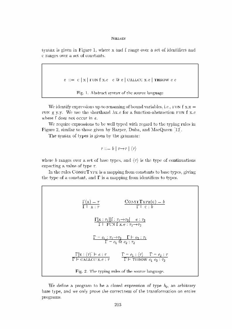
Nielsen

syntax is given in Figure 1, where x and f range over a set of identi�ers and

c ranges over a set of constants.

e ::= c j x j fun f x:e j e @ e j callcc x:e j throw e e

Fig. 1. Abstract syntax of the source language

We identify expressions up to renaming of bound variables, i.e., fun f x:x =

fun g y:y. We use the shorthand �x:e for a function-abstraction fun f x:e

where f does not occur in e.

We require expressions to be well typed with regard to the typing rules in

Figure 2, similar to those given by Harper, Duba, and MacQueen [12].

The syntax of types is given by the grammar:

� ::= b j �!� j h�i

where b ranges over a set of base types, and h�i is the type of continuations

expecting a value of type �.

In the rules ConstType is a mapping from constants to base types, giving

the type of a constant, and � is a mapping from identi�ers to types.

�(x) = �

� ` x : �ConstType(c) = b

� ` c : b

�[x : �1][f : �1!�2] ` e : �2� ` fun f x:e : �1!�2

� ` e1 : �1!�2 � ` e2 : �1� ` e1 @ e2 : �2

�[x : h�i] ` e : �� ` callcc x:e : �

� ` e1 : h�i � ` e2 : �� ` throw e1 e2 : �2

Fig. 2. The typing rules of the source language.

We de�ne a program to be a closed expression of type b0, an arbitrary

base type, and we only prove the correctness of the transformation on entire

programs.

203

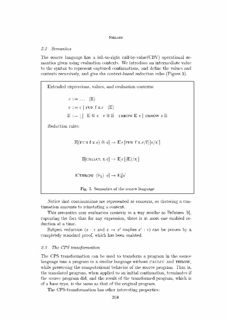
Nielsen

2.2 Semantics

The source language has a left-to-right call-by-value(CBV) operational se-

mantics given using evaluation contexts. We introduce an intermediate value

to the syntax to represent captured continuations, and de�ne the values and

contexts recursively, and give the context-based reduction rules (Figure 3).

Extended expressions, values, and evaluation contexts:

e ::= : : : j hEi

v ::= c j fun f x:e j hEi

E ::= [ ] j E @ e j v @ E j throw E e j throw v E

Reduction rules:

E[(fun f x:e) @ v] ! E[e [fun f x:e=f] [v=x]]

E[callcc x:e] ! E[e [hEi=x]]

E[throw hE1i v] ! E1[v]

Fig. 3. Semantics of the source language

Notice that continuations are represented as contexts, so throwing a con-

tinuation amounts to reinstating a context.

This semantics uses evaluation contexts in a way similar to Felleisen [9],

capturing the fact that for any expression, there is at most one enabled re-

duction at a time.

Subject reduction (e : � and e ! e 0 implies e 0 : �) can be proven by a

completely standard proof, which has been omitted.

2.3 The CPS transformation

The CPS transformation can be used to transform a program in the source

language into a program in a similar language without callcc and throw,

while preserving the computational behavior of the source program. That is,

the translated program, when applied to an initial continuation, terminates if

the source program did, and the result of the transformed program, which is

of a base type, is the same as that of the original program.

The CPS-transformation has other interesting properties:

204

Nielsen

� It generates programs that can be evaluated under both a call-by-name

(CBN) and a CBV semantics and yield the same result, which corresponds

to the result of the source program. A number of CPS transformations exist,

each corresponding to an evaluation-order for the source language [13].

� It generates programs where all applications are tail-calls, i.e., no applica-

tion is in an argument position.

CPS transformations are used in many places, but primarily in compilers

to give an intermediate representation [1,21] and as a way to simplify the

language of a program before applying other transformations or analyses to

it [4]. It is the last application that is the motivation for the present work.

The standard CBV CPS transformation is de�ned in Figure 4.

C[[c]] = �k:k @ Cv[[c]])

C[[x]] = �k:k @ Cv[[x]])

C[[fun f x:e]] = �k:k @ Cv[[fun f x:e]])

C[[e1 @ e2]] = �k:C[[e1]] @ �v:C[[e2]] @ �v0:v @ v0 @ k

C[[callcc x:e]] = �k:�x:C[[e]] @ k @ k

C[[throw e1 e2]] = �k:C[[e1]] @ �v:C[[e2]] @ v

Cv[[x]]) = x

Cv[[c]]) = c

Cv[[fun f x:e]]) = fun f x:C[[e]]

Fig. 4. The CPS transformation

The Cv[[�]]) function is used to coerce values and identi�ers into CPS form,

which consists of transforming the bodies of function abstractions. Values

and identi�ers share the property that Reynolds called \being trivial" [19]

and Moggi called \being a value" (as opposed to a computation) [16], in

the sense that they have no computational e�ects, including nontermination.

The C[[�]] function is used on expressions with potential e�ects, the \serious"

expressions.

205

Nielsen

3 The selective CPS transformation

As stated in the previous section, we treat trivial and serious expressions dif-

ferently. Trivial expressions are those that have no computational e�ects and

serious expressions are those that might have e�ects. The safe approximation

used by the standard CPS transformation assumes that any application might

have e�ects, which is not unreasonable when one considers nontermination as

an e�ect.

In the source language we have added control e�ects, and it makes sense

only to focus on those, and let the termination behavior be preserved by only

evaluating the result in a CBV semantics. If we do that, we can use an e�ect

analysis to �nd the parts of the program that are guaranteed to be free of

the control e�ects generated by callcc and throw. In the following we

will use the words \trivial" and \non-trivial" about the absence or possible

presence of control e�ects only, while ignoring the partiality e�ect of non-

termination. That is, an expression that has an in�nite reduction sequence

can still be said to be \trivial" with regards to control e�ects. We are not

aiming for evaluation-order independence, rather the source and target lan-

guages are assumed to have the same evaluation-order (call-by-value), so the

translation need not take any measures to preserve or prevent non-termination

in otherwise e�ect-free expressions.

This section de�nes e�ect-annotated expressions, an e�ect type system to

check the consistency of the annotation, and a selective CPS transformation

that keeps trivial applications in direct style.

3.1 Annotated source language

We annotate a program with annotations taken from the set fT;Ng, which

is a partial order with the ordering relation N < T.

We mark some applications as trivial, with a T, and some as (potentially)

non-trivial, with an N. The trivial ones are kept in direct style, and as such

do not expect to receive a continuation.

For an expression, an e�ect analysis can tell us one of three things:

� Some evaluation of the expression will certainly give rise to e�ects (meaning,

in this case, the reduction sequence of the expression contains evaluations

of callcc or throw expressions),

� no evaluation of the expression will give rise to e�ects, or

� we just don't know either way, which can happen since the problem is

generally undecidable.

The present transformation aims to keep the expressions in the second case

in direct style. Since any e�ectful expression must be put into CPS, we must

treat the �rst and third cases equally, and they are both marked N. Unifying

these two cases gives rise to the stated ordering where greater means more

206

Nielsen

information is known: certainty of the absence of e�ects as opposed to only

possible presence.

A ::= T j N

e ::= c j x j funA f x:e j (e @A e)A j callcc x:e j throw e e

These are the minimal annotations needed for our purpose. We treat values

and identi�ers (the traditional trivial expressions) as if they were annotated

as such, i.e., (e)T is a match for any trivial expression, just as (e)N matches

the two control operators.

We require that an expression annotated as trivial actually is so, i.e., when-

ever it is evaluated, the reduction sequence contains no steps corresponding to

reductions of callcc or throw expressions. Since we use this annotation as

a basis for the selective CPS transformation, we will want to CPS transform

all expressions that are not marked trivial.

We have to treat functions and applications with special care. When a

lambda abstraction is applied at an application point, the body of the abstrac-

tion is also evaluated at that point. If the body is not trivial, then neither

is the application, and after selective CPS transformation, the transformed

application must pass a continuation to the transformed body, and the body

should expect a continuation.

In a higher-order program, more than one abstraction can be applied at

the same application point, and after transformation, all of these abstractions

must either expect a continuation or not. That means that all functions that

can end up in a given application must be transformed in the same way. That

divides the abstractions into two groups, those transformed into CPS, i.e.,

expecting a continuation, and those kept in direct style, i.e., not expecting a

continuation. Some abstractions with a trivial body might be transformed to

expect a continuation in order to match the other abstractions that reach the

same application points.

We will say that the annotation is \consistent" (with regards to the be-

havior of the program) if:

� All expressions marked trivial are trivial,

� all abstractions marked trivial, or non-trivial, are only applied at application

points marked trivial, or non-trivial respectively, and

� all abstractions whose body are marked non-trivial, are themselves marked

as non-trivial.

To check all this, we use an extension of the type system to an e�ect type

system that guarantees that the annotation is consistent. The types are also

207

Nielsen

annotated, so the grammar of types is:

� ::= b j �A!� j h�i

The e�ect system is shown in Figure 5.

�(x) = �

� ` x : �;TConstType(c) = b

� ` c : b;T

�[x : �1][f : (�1A1

!�2)] ` e : �2;A A1 � A

� ` fun f x:e : �1A1

!�2;T

� ` e1 : �1A3

!�2;A1 � ` e2 : �1;A2 A � min(A1;A2;A3)� ` e1 @ e2 : �2;A

�[x : h�i] ` e : �;A� ` callcc x:e : �;N

� ` e1 : h�i ;A1 � ` e2 : �;A2

� ` throw e1 e2 : �2;N

Fig. 5. E�ect type system

If an expression is typeable in the original type system, then there exists

at least one annotation that is typeable in the e�ect system, namely the one

where all functions and applications are marked non-trivial.

The � in the rule for function abstractions is exactly due to the restriction

on which functions that can ow where. Functions with trivial bodies can be

annotated with an N, allowing them to ow into an application expecting to

pass a continuation, but this is re ected in the type, which is the only thing

that is known at the application point. There are two di�erent annotated

function types, one for each annotation, and only one of these is allowed at

each application point.

The � on the rule for applications is discussed in the next section,

We only consider well-annotated expressions from here on, i.e., expressions

that are allowed by the e�ect typing rules.

3.2 The Selective CPS Transformation

We de�ne a CPS transformation that transforms well-annotated expressions

and leaves trivial applications in direct style (Figure 6).

208

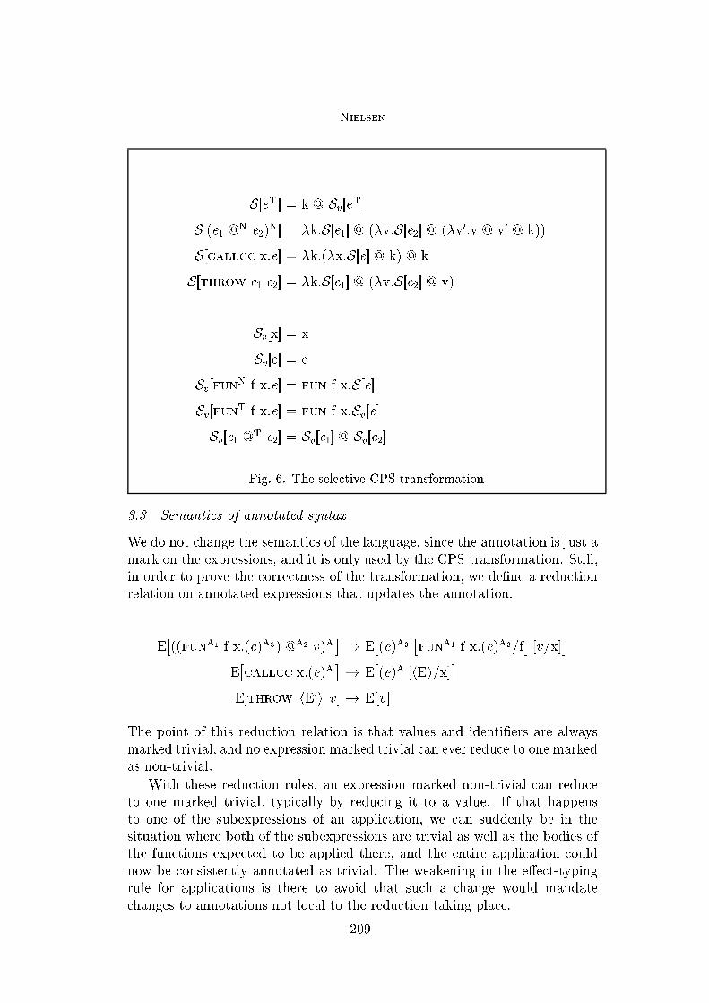
Nielsen

S[[eT ]] = k @ Sv[[eT ]]

S[[(e1 @N e2)

N]] = �k:S[[e1]] @ (�v:S[[e2]] @ (�v0:v @ v0 @ k))

S[[callcc x:e]] = �k:(�x:S[[e]] @ k) @ k

S[[throw e1 e2]] = �k:S[[e1]] @ (�v:S[[e2]] @ v)

Sv[[x]] = x

Sv[[c]] = c

Sv[[funN f x:e]] = fun f x:S[[e]]

Sv[[funT f x:e]] = fun f x:Sv[[e]]

Sv[[e1 @T e2]] = Sv[[e1]] @ Sv[[e2]]

Fig. 6. The selective CPS transformation

3.3 Semantics of annotated syntax

We do not change the semantics of the language, since the annotation is just a

mark on the expressions, and it is only used by the CPS transformation. Still,

in order to prove the correctness of the transformation, we de�ne a reduction

relation on annotated expressions that updates the annotation.

E�((funA1 f x:(e)A3) @A2 v)A

�! E

�(e)A3

�funA1 f x:(e)A3=f

�[v=x]

�

E�callcc x:(e)A

�! E

�(e)A [hEi=x]

�

E[throw hE0i v] ! E0[v]

The point of this reduction relation is that values and identi�ers are always

marked trivial, and no expression marked trivial can ever reduce to one marked

as non-trivial.

With these reduction rules, an expression marked non-trivial can reduce

to one marked trivial, typically by reducing it to a value. If that happens

to one of the subexpressions of an application, we can suddenly be in the

situation where both of the subexpressions are trivial as well as the bodies of

the functions expected to be applied there, and the entire application could

now be consistently annotated as trivial. The weakening in the e�ect-typing

rule for applications is there to avoid that such a change would mandate

changes to annotations not local to the reduction taking place.

209

Nielsen

All these properties make a proof of Subject Reduction a trivial extension

of the proof for the unannotated syntax.

One reason for having both annotations and an e�ect system, and not,

e.g., only the e�ect system, is for ease of representation. Even if a reduced

program allows a more precise e�ect-analysis than the original program, the

transformation is based on the original program, and the annotation keeps the

original annotation throughout the reduction sequence.

4 Proof of correctness

To prove the correctness of the transformation, we must �rst specify a notion

of correctness. In this case we require that the transformed program reduces

to the same result as the original program.

Theorem 4.1 (Correctness of the Selective CPS Transformation) If e

is a closed and well-annotated expression of type b0 then

e !� v , S[[e]] @ (�x:x) !� v

In Plotkin's original proof, the result of the transformed program would be

Sv[[v]], but since the program has a type where the only values are constants,

and all constants satisfy Sv[[c]] = c, we can state the theorem as above.

4.1 The selective colon-translations

The proof uses a method similar to Plotkin's in his original proof of the correct-

ness of the CPS transformation [17]. It uses a so-called \colon-translation" to

bypass the initial administrative reductions and focus on the evaluation point.

The intuition that drives the normal CPS transformation is that if e re-

duces to v then (C[[e]] @ k) should evaluate to (k @ Cv[[v]])). Plotkin captured

this in his colon translation where if e ! e 0 then e : k !� e 0 : k, and at the

end of the derivation, values satis�ed v : k = k @ (v), where (�) is what

we write Sv[[�]].

The idea of the colon translation is that in e : k, the k represents the

context of e, which in the transformed program has been collected in a contin-

uation: a function expecting the result of evaluating e. The colon separates

the source program to the left and the transformed program to the right of it.

In the selective CPS transform, some contexts are not turned into continua-

tions, namely the contexts of expressions marked trivial, since such expressions

are not transformed to CPS expressions, and as such does not expect a con-

tinuation.

Therefore we have two colon translations, one for non-trivial expressions,

with a continuation function after the colon, and one for trivial expressions

with an evaluation context after the colon. The de�nition is shown in Figure 7.

In both cases, what is to the left of the colon is a piece of source syntax, and

210

Nielsen

what is to the right is a representation of the context of that expression in the

source program translated to the target language. If the expression is trivial,

the source context is represented by a context in the target language, and

the translation of the expression is put into this context. If the expression is

not trivial, then the source context is represented by a continuation function

which is passed to the translation of the expression.

eT : k = eT : [k @ [ ]]

(e1 @N e2)

N : k = e1 : �v:S[[e2]] @ (�v0:v @ v0 @ k) if e1 is not a value

(v1 @N e2)

N : k = e2 : �v0:Sv[[v1]] @ v0 @ k if e2 is not a value

(v1 @N v2)

N : k = Sv[[v1]] @ Sv[[v2]] @ k

(e1 @T e2)

N : k = e1 : �v:S[[e2]] @ (�v0:k @ (v @ v0)) if e1 is not a value

(v1 @T e2)

N : k = e2 : �v0:k @ (Sv[[v1]] @ v0) if e2 is not a value

(v1 @T v2)

N : k = k @ (Sv[[v1]] @ Sv[[v2]])

callcc x:e : k = (�x:S[[e]] @ k) @ k

throw e1 e2 : k = e1 : �v:S[[e2]] @ v if e1 is not a value

throw v1 e2 : k = e2 : Sv[[v1]] if e2 is not a value

throw v1 v2 : k = Sv[[v1]] @ Sv[[v2]]

x : E = E[x]

c : E = E[c]

funN f x:e : E = E[fun f x:S[[e]]]

funT f x:e : E = E[fun f x:Sv[[e]]]

(e1 @T e2)

T : E = e1 : E�([ ] @T Sv[[e2]])

T�

if e1 is not a value

(v1 @T e2)

T : E = e2 : E�(Sv[[v1]] @

T [ ])T�

if e2 is not a value

(v1 @T v2)

T : E = E�(Sv[[v1]] @

T Sv[[v2]])T�

Fig. 7. The selective colon translation on expressions

In Plotkin's colon translation, v : k = k @ �(v). This also holds for

this colon translation pair, since v : k = v : [k @ [ ]], since v is trivial, and

v : [k @ [ ]] = k @ v by the de�nition of the e : E-translation.

211

Nielsen

The e : E-translation is not as signi�cant as the e : k-translation, since all

it does is apply the -function to the argument, i.e., if e is a trivial expression

then e : E = E[Sv[[e]]]. There are no administrative reductions to bypass in

direct style.

We plan to use the colon translations on the result of reducing on the

annotated expressions, so we extend it to work on continuation values, hEi,

which are values and as such trivial.

hE0i : E = E[E0 : id]

where id = �x:x and E : k de�nes either a continuation function or a context

as displayed in Figure 8, where ET represents any non-empty context with a

top-most annotation as trivial.

[ ] : k = k

ET : k = ET : [k @ [ ]]

(E @N e2)N : k = E : �v:S[[e2]] @ (�v0

:v @ v0 @ k)

(E @T e2)N : k = E : �v:S[[e2]] @ (�v0

:k @ (v @ v0))

(v1 @N E)N : k = E : (�v0

:Sv[[v1]] @ v0 @ k)

(v1 @T E)N : k = E : (�v0

:k @ (Sv[[v1]] @ v0))

throw E e2 : k = E : �v:S[[e2]] @ v

throw v1 E : k = E : Sv[[v1]]

[ ] : E = E

(E @T e2)T : E0 = E : E0[[ ] @ Sv[[e2]]]

(v1 @T E)T : E0 = E : E0[Sv[[v1]] @ [ ]]

Fig. 8. The selective colon translation on contexts.

The E : k-translation yields either continuation functions or contexts, de-

pending on the annotation of the innermost levels of the context argument,

and the E : E-translation always gives a context, but requires that the �rst

argument's outermost annotation is trivial.

These colon-translations satisfy a number of correspondences.

Proposition 4.2 For all contexts E1, E2, and E3, and continuation functions

212

Nielsen

(closed functional values) the following equalities hold.

E1[E2[ ]] : k = E2 : (E1 : k)

E1[E2[ ]] : E3 = E2 : (E1 : E3)

Proof. The proof is by simple induction on the context E1.

� If E1 = [ ] then (E1[E2[ ]] : k) = (E2 : k) = (E2 : (E1 : k)) and (E1[E2[ ]] :

E3) = (E2 : E3) = (E2 : (E1 : E3)).

� If E1 =�(E @N e2)

N�then

E1[E2[ ]] : k = (E[E2] @N e2)

N : k

= E[E2] : �v:S[[e2]] @ (�v0:v @ v0 @ k) (def. of E : k)

= E2 : (E : �v:S[[e2]] @ (�v0:v @ v0 @ k)) (I.H.)

= E2 : (�(E @N e2)

N�: k) (def. E : k)

� The remaining cases are similar.

2

One would expect that similar equalities hold for the colon translations

on expressions, i.e., E[e] : k = e : (E : k) and E[e] : E0 = e : (E : E0), and

indeed these equalities hold in most cases. The exception is when E is non-

empty and the \innermost" expression of the context is not annotated as

trivial, e.g., E1

�([ ] @ e1)

N�for some context E1 and expression e1, and e

is a value. Normally the e : k translation descends the left-hand side and

rebuilds the context on the right hand side, either as a continuation function

or as a context, depending on the annotation. The exception mentioned,

E[e] : k, the focus of the colon translation, the expression on the left hand

side of the colon, would never descend all the way down to a value. We have

made special cases for v @ e to bypass administrative reductions, so E[v] : k

would not equal v : (E : k), because the latter introduces an administrative

reduction. Reducing that administrative reduction, applying k to Sv[[v]], does

lead to v : (E : k) again in one or more reduction steps. That is, if e is a value

and E is not a trivial context then e : (E : k) = (E : k) @ Sv[[e]] !� E[e] : k,

and likewise for the e : E-relation.

Proposition 4.3 For all contexts E and E0, expressions e, and continuation

functions k

e : (E : k) !� E[e] : k

e : (E : E0) !� E[e] : E0 (if e trivial)

and !� is !0, i.e., equality, if e is not a value.

213

Nielsen

Proof. Omitted. 2

4.2 Colon-translation lemmas

Plotkin used four lemmas to prove his simulation and indi�erence theorems.

We only prove simulation, which corresponds to Plotkin's simulation, since we

already know that indi�erence does not hold for a selective CPS transforma-

tion (at least unless the selectivity is based on the e�ect of nontermination as

well).

Lemma 4.4 (Substitution) If �[x : �1] ` e : �2;A and ` v : �1;T is a closed

value then

S[[e]] [Sv[[v]]=x] = S[[e [v=x]]]

Sv[[e]] [Sv[[v]]=x] = Sv[[e [v=x]]] (if e is trivial)

Proof. The proof is by induction on the structure of e, using the distributive

properties of substitution and taking the trivial cases before the non-trivial

ones (because the S[[�]] translation defers trivial subexpressions to the trans-

formation). The details have been omitted. 2

Lemma 4.5 (Initial reduction) If � ` e : �;A and k is a continuation

function of appropriate type then

S[[e]] @ k !� e : k

E[Sv[[e]]] = e : E (if e is trivial)

Proof. Again, the proof is by induction on the structure of e with the S[[�]]

case taken after the case for trivial expressions.

The E[Sv[[�]]] = � : E case: There are four cases covering all trivial expressions:� If e is a value or an identi�er then e : E = E[Sv[[e]]] by de�nition of e : E.� If e = (e1 @

T e2)T (e1 not a value) then

(e1 @T e2)

T : E = e1 : E[[ ] @ Sv[[e2]]] (def. e : E)

= E[Sv[[e1]] @ Sv[[e2]]] (I.H.)

= E�Sv[[(e1 @

T e2)T ]]�(def. )

� If e = (v1 @T e2)

T (e2 not a value) then

(v1 @T e2)

T : E = e2 : E[Sv[[v1]] @ [ ]] (def. e : E)

= E[Sv[[v1]] @ Sv[[e2]]] (I.H.)

= E�Sv[[(v1 @

T e2)T ]]�(def. )

214

Nielsen

� If e = (v1 @T v2)

T then

(v1 @T v2)

T : E = E[Sv[[v1]] @ Sv[[v2]]] (I.H.)

= E�Sv[[(v1 @

T v2)T ]]�(def. )

This accounts for all trivial expressions.

The S[[�]] @ k !� � : k case: There is one sub-case for each non-trivial expres-

sion, and one case for all trivial expressions:� If e is trivial then S[[e]] @ k = k @ Sv[[e]] = e : [k @ [ ]] = e : k from the

above cases and the de�nition of e : k.� If e = (e1 @

N e2)N (e1 not a value) then

S[[(e1 @N e2)

N ]] @ k

! S[[e1]] @ (�v:S[[e2]] @ (�v0:v @ v0 @ k)) (def. S[[�]])

!� e1 : (�v:S[[e2]] @ (�v0:v @ v0 @ k)) (I.H.)

= (e1 @N e2)

N : k (def. e : k)

� If e = (v1 @N e2)

N (e2 not a value) then

S[[(v1 @N e2)

N]] @ k

! S[[v1]] @ (�v:S[[e2]] @ (�v0:v @ v0 @ k)) (def. S[[�]])

! (�v:S[[e2]] @ (�v0:v @ v0 @ k)) @ Sv[[v1]] (def. S[[v]])

! S[[e2]] @ (�v0:Sv[[v1]] @ v0 @ k)

!� e2 : �v0:Sv[[v1]] @ v0 @ k (I.H.)

= (v1 @N e2)

N : k (def. e : k)

� If e = (v1 @N v2)

N then the proof is similar to the previous case except

two values need to be applied to continuations instead of just one.� If e = (e1 @T e2)

N then the proofs are similar to the ones for e =

(e1 @T e2)N except that the innermost application is k @ (v @ v0) in-

stead of (v @ v0) @ k.� If e = callcc x:e1 then S[[callcc x:e1]] @ k ! (�x:S[[e1]] @ k) @ k =

callcc x:e1 : k.� If e = throw e1 e2 the proofs are similar to the ones for application.

2

Lemma 4.6 (Simulation) If E[e] ! E0[e 0] is one of the reduction rules for

the annotated language, then

E[e] : id!� E0[e 0] : id

215

Nielsen

and if the reduction is not of a throw expression, then the !� is actually

one or more steps.

Proof. Counting annotations, there are �ve cases:

� If e = (funN f x:e1 @N v)N then

E�(funN f x:e1 @

N v)N�: id

= (funN f x:e1 @N v)N : (E : id) (Prop. 4.3)

= Sv[[funN f x:e1]] @ Sv[[v]] @ (E : id) (def. e : k)

= fun f x:S[[e1]] @ Sv[[v]] @ (E : id) (def. )

! S[[e1]]�Sv[[fun

N f x:e1]]=f�[Sv[[v]]=x] @ (E : id)

= S[[e1�funN f x:e1=f

�[v=x]]] @ (E : id) (Lemma 4.4)

!� e1�funN f x:e1=f

�[v=x] : (E : id) (Lemma 4.5)

!� E�e1

�funN f x:e1=f

�[v=x]

�: id (Prop. 4.3)

� If e = (funT f x:e1 @T v)N then we know that e1 is trivial, since otherwise

the function would be annotated N, and E : k is a continuation since E has

no trivial inner sub-contexts.

E�(funT f x:e1 @

T v)N�: id

= (funT f x:e1 @T v)N : (E : id) (Prop. 4.3)

= (E : id) @ (Sv[[funT f x:e1]] @ Sv[[v]]) (def. e : k)

= (E : id) @ (fun f x:Sv[[e1]] @ Sv[[v]]) (def. )

! (E : id) @ Sv[[e1]]�Sv[[fun

T f x:e1]]=f�[Sv[[v]]=x]

= (E : id) @ Sv[[e1�funT f x:e1=f

�[v=x]]] (Lemma 4.4)

!� e1�funT f x:e1=f

�[v=x] : [(E : id) @ [ ]] (Lemma 4.5, e1 trivial)

= e1�fun

T f x:e1=f�[v=x] : (E : id) (def. e : k)

!� E�e1

�funN f x:e1=f

�[v=x]

�: id (Prop. 4.3)

� If e = (e1 @T e2)

T then either E : k is a context or a continuation. If it is a

continuation the proof proceeds just as the previous case. If it is a context

216

Nielsen

then

E�(funT f x:e1 @

T v)T�: id

= (funT f x:e1 @T v)T : (E : id) (Prop. 4.3)

= (E : id)�Sv[[fun

T f x:e1]] @ Sv[[v]]�

(def. e : k)

= (E : id)[fun f x:Sv[[e1]] @ Sv[[v]]] (def. )

! (E : id)�Sv[[e1]]

�Sv[[fun

T f x:e1]]=f�[Sv[[v]]=x]

�

= (E : id)�Sv[[e1

�funT f x:e1=f

�[v=x]]]

�(Lemma 4.4)

!� e1�funT f x:e1=f

�[v=x] : (E : id) (Lemma 4.5, e1 trivial)

!� E�e1

�funN f x:e1=f

�[v=x]

�: id (Prop. 4.3)

� If e = callcc x:e1 then

E[callcc x:e1] : id

= callcc x:e1 : (E : id) (Prop. 4.3)

= (�x:S[[e1]] @ (E : id)) @ (E : id) (def. e : k)

! S[[e1]] @ (E : id) [(E : id)=x]

= S[[e1]] [(E : id)=x] @ (E : id) (E : k is closed)

= S[[e1]] [Sv[[hEi]]=x] @ (E : id) (def. Sv[[hEi]])

= S[[e1 [hEi=x]]] @ (E : id) (Lemma 4.4)

!� e1 [hEi=x] : (E : id) (Lemma 4.5)

!� E[e1 [hEi=x]] : id (Prop. 4.3)

� If e = throw hE0i v then

E[throw hE0i v] : id = Sv[[hE0i]] @ Sv[[v]] (def. e : k)

= (E0 : id) @ Sv[[v]] (def. Sv[[hEi]])

= v : [( @ E0 : id)[ ]] (def. v : E)

= v : (E0 : id) (def. (e)T : k)

!� E0[v] : id (Prop. 4.3)

In all cases except throw, there is at least one reduction step.

2

217

Nielsen

4.3 Proof of correctness

To prove the correctness of the selective CPS transformation, we use the sim-

ulation lemma in two ways.

Proof. The proof of e !� c =) S[[e]] @ id !� c follows directly from the

lemma 4.5 and repeated use of lemma 4.6. Assume e !� c.

S[[e]] @ id !� e : id (Lemma 4.5)

!� c : id (Lemma 4.6, repeated)

= c : [id @ [ ]] (def. (e)T : k)

= id @ c (def. c : E)

! c

.

The other direction of correctness, S[[e]] @ id !� c =) e !� c, is shown

by contraposition. Assuming that for no c does e !� c, that is, e diverges,

allows us to show that the same holds for S[[e]].

The proof that transformation preserves divergence also follow from Lem-

mas 4.5 and 4.6. Since S[[e]] @ id !� e : id it suÆces to show that e : id has

an arbitrary long reduction sequence.

Assume that e diverges. We show that for any n there exists an m such

that if e !m e1 then (e : id)!� (e1 : id) in n or more reduction steps.

This is proven by induction on n. The base case (n = 0) is trivial. For the

induction case (n + 1) look at the n case. There exists m such that e !m e1and e : id!� e1 : id. Look at the reduction sequence from e1.

� If the �rst reduction step (e1 ! e2) is not the reduction of a throw ex-

pression, then e1 : id !+ e2 : id, and m + 1 gives us our n + 1 or longer

reduction sequence of e : id.

� If the �rst reduction step (e1 ! e2) is of a throw expression, then e1 :

id!� e2 : id. In that case we look at the next step in the same way. Either

we �nd a reduction that is not a throw, and we get the m needed for

the proof, or there is nothing but reductions of throw expressions in the

in�nite reduction sequence of e1.

There can not be an in�nite sequence of reductions of throw expressions,

since reducing a throw expression necessarily reduces the size of the entire

program. A substitution into a context corresponds to the application of a

linear function, and it reduces the size of the expression if one counts it as,

e.g., number of distinct subexpressions or number of throw-expressions.

That means that e : id has an in�nite reduction sequence. 2

218

Nielsen

5 Conclusion

We have proven the correctness of a selective CPS transformation based on an

e�ect analysis. Similar proofs can be made for other �-encodings and compu-

tational e�ects (e.g., with monads), where the immediate choice would be the

e�ect of non-termination. That is the e�ect that is encoded by the traditional

CPS transformation of languages with no other e�ects, and if one has an an-

notation of such a program, marking terminating (e�ect-free) expressions to

keep in direct style, then the method works just as well.

5.1 Perspectives

Danvy and Hatcli�'s CPS transformation after strictness analysis [6] general-

izes the call-by-name and the call-by-value CPS transformations. The same

authors' CPS transformation after totality analysis [7] generalizes the call-

by-name CPS transformation and the identity transformation. In the same

manner, the present work generalizes the call-by-value CPS transformation

and the identity transformation, and proves this generalization correct.

Danvy and Filinski introduced the one-pass CPS-transformation [5] that

removes the administrative reductions from the result by performing them

at transformation time. This optimization can be applied to the selective

CPS-transformation presented here as well. A proof of the correctness of the

one-pass CPS-transformation also using Plotkin's colon translation exists [8].

We expect that the methods used for proving correctness of the selective- and

the one-pass CPS transformations are orthogonal, and can easily be combined.

The selective CPS transformation presented here is based on an e�ect

analysis and should generalize to other computational e�ects than control,

e.g., state or I/O. The proof will not carry over to other e�ects, since it relies

on the choice of �-encoding of the e�ect primitives, but we expect that the

structure of the proof can be preserved.

The approach taken is \Curry-style" in the sense that we have given a lan-

guage and its operational meaning, and only after the fact we have associated

types and e�ect annotation to the untyped terms. A \Church-style" approach,

such as Filinski's [10,11], would have de�ned the language with explicit types

and e�ect annotation, so that only well-typed, consistently annotated pro-

grams are given a semantics.

5.2 Future work

It is possible to prove results similar to the present ones for other choices of

e�ects and combinations of e�ects. A sensible choice would be a monadic

e�ect of state and control, since it is suÆcient to implement all other choices

of layered monads [11]. A proof similar to the present one for both state and

control e�ects would be a logical next step.

219

Nielsen

Acknowledgments:

The method of extending the colon translation to selective CPS transformation

was originally developed in cooperation with Junk-taek Kim and Kwangkeun

Yi from KAIST in Korea, and with Olivier Danvy from BRICS in Denmark.

The present work would not have been possible without their inspiration.

Thanks are also due to Andrzej Filinski and to the anonymous referees for

their comments.

References

[1] AndrewW. Appel. Compiling with Continuations. Cambridge University Press,

New York, 1992.

[2] Hans-J. Boehm, editor. Proceedings of the Twenty-First Annual ACM

Symposium on Principles of Programming Languages, Portland, Oregon,

January 1994. ACM Press.

[3] William Clinger, Daniel P. Friedman, and Mitchell Wand. A scheme for a

higher-level semantic algebra. In John Reynolds and Maurice Nivat, editors,

Algebraic Methods in Semantics, pages 237{250. Cambridge University Press,

1985.

[4] Daniel Damian and Olivier Danvy. Syntactic accidents in program analysis. In

Philip Wadler, editor, Proceedings of the 2000 ACM SIGPLAN International

Conference on Functional Programming, pages 209{220, Montr�eal, Canada,

September 2000. ACM Press.

[5] Olivier Danvy and Andrzej Filinski. Representing control, a study of the CPS

transformation. Mathematical Structures in Computer Science, 2(4):361{391,

December 1992.

[6] Olivier Danvy and John Hatcli�. CPS transformation after strictness analysis.

ACM Letters on Programming Languages and Systems, 1(3):195{212, 1993.

[7] Olivier Danvy and John Hatcli�. On the transformation between direct and

continuation semantics. In Stephen Brookes, Michael Main, Austin Melton,

Michael Mislove, and David Schmidt, editors, Proceedings of the 9th Conference

on Mathematical Foundations of Programming Semantics, number 802 in

Lecture Notes in Computer Science, pages 627{648, New Orleans, Louisiana,

April 1993. Springer-Verlag.

[8] Olivier Danvy and Lasse R. Nielsen. A higher-order colon translation. In

Herbert Kuchen and Kazunori Ueda, editors, Fifth International Symposium on

Functional and Logic Programming, number 2024 in Lecture Notes in Computer

Science, pages 78{91, Tokyo, Japan, March 2001. Springer-Verlag. Extended

version available as the technical report BRICS RS-00-33.

[9] Matthias Felleisen. The Calculi of �-v-CS Conversion: A Syntactic Theory of

Control and State in Imperative Higher-Order Programming Languages. PhD

220

Nielsen

thesis, Department of Computer Science, Indiana University, Bloomington,

Indiana, August 1987.

[10] Andrzej Filinski. Representing monads. In Boehm [2], pages 446{457.

[11] Andrzej Filinski. Representing layered monads. In Alex Aiken, editor,

Proceedings of the Twenty-Sixth Annual ACM Symposium on Principles of

Programming Languages, pages 175{188, San Antonio, Texas, January 1999.

ACM Press.

[12] Robert Harper, Bruce F. Duba, and David MacQueen. Typing �rst-class

continuations in ML. Journal of Functional Programming, 3(4):465{484,

October 1993.

[13] John Hatcli� and Olivier Danvy. A generic account of continuation-passing

styles. In Boehm [2], pages 458{471.

[14] Jung-taek Kim and Kwangkeun Yi. Interconnecting Between CPS Terms and

Non-CPS Terms. In Sabry [20].

[15] Jung-taek Kim, Kwangkeun Yi, and Olivier Danvy. Assessing the overhead

of ML exceptions by selective CPS transformation. In Greg Morrisett, editor,

Record of the 1998 ACM SIGPLAN Workshop on ML and its Applications,

Baltimore, Maryland, September 1998. Also appears as BRICS technical report

RS-98-15.

[16] Eugenio Moggi. Computational lambda-calculus and monads. In Proceedings

of the Fourth Annual IEEE Symposium on Logic in Computer Science, pages

14{23, Paci�c Grove, California, June 1989. IEEE Computer Society Press.

[17] Gordon D. Plotkin. Call-by-name, call-by-value and the �-calculus. Theoretical

Computer Science, 1:125{159, 1975.

[18] John Reppy. Local CPS conversion in a direct-style compiler. In Sabry [20].

[19] John C. Reynolds. De�nitional interpreters for higher-order programming

languages. Higher-Order and Symbolic Computation, 11(4):363{397, 1998.

Reprinted from the proceedings of the 25th ACM National Conference (1972).

[20] Amr Sabry, editor. Proceedings of the Third ACM SIGPLAN Workshop on

Continuations CW'01, number 545 in Technical Report, Computer Science

Department, Indiana University, Bloomington, Indiana, December 2000.

[21] Guy L. Steele Jr. Rabbit: A compiler for Scheme. Technical Report AI-TR-

474, Arti�cial Intelligence Laboratory, Massachusetts Institute of Technology,

Cambridge, Massachusetts, May 1978.

221

Nielsen

222

MFPS 17 Preliminary Version

Semantics for Algebraic Operations

Gordon Plotkin and John Power 1

Laboratory for the Foundations of Computer Science

University of Edinburgh

King's Buildings

Edinburgh EH9 3JZ

SCOTLAND

Abstract

Given a category C with �nite products and a strong monad T on C, we in-

vestigate axioms under which an ObC-indexed family of operations of the form

�x : (Tx)n�! Tx provides a de�nitive semantics for algebraic operations added to

the computational �-calculus. We recall a de�nition for which we have elsewhere

given adequacy results for both big and small step operational semantics, and we

show that it is equivalent to a range of other possible natural de�nitions of algebraic

operation. We outline examples and non-examples and we show that our de�nition

is equivalent to one for call-by-name languages with e�ects too.

1 Introduction

Eugenio Moggi, in [6,8], introduced the idea of giving a uni�ed category theo-retic semantics for computational e�ects such as nondeterminism, probabilis-

tic nondeterminism, side-e�ects, and exceptions, by modelling each of them

uniformly in the Kleisli category for an appropriate strong monad on a basecategory C with �nite products. He supported that construction by develop-

ing the computational �-calculus or �c-calculus, for which it provides a soundand complete class of models. The computational �-calculus is essentially the

same as the simply typed �-calculus except for the essential fact of making

a careful systematic distinction between computations and values. However,it does not contain operations, and operations are essential to any program-

ming language. So here, in beginning to address that issue, we provide a

uni�ed semantics for algebraic operations, supported by equivalence theorems

to indicate de�nitiveness of the axioms.

1 This work is supported by EPSRC grant GR/L89532: Notions of computability for gen-

eral datatypes.

This is a preliminary version. The �nal version will be published inElectronic Notes in Theoretical Computer Science

URL: www.elsevier.nl/locate/entcs

Plotkin and Power

We distinguish here between algebraic operations and arbitrary operations.

The former are, in a sense we shall make precise, a natural generalisation, from

Set to an arbitrary category C with �nite products, of the usual operations

of universal algebra. The key point is that the operations

�x : (Tx)n �! Tx

are parametrically natural in the Kleisli category for a strong monad T on

C, as made precise in De�nition 2.1: in that case, we say that the monad

T supports the operations; the leading class of examples has T being gener-

ated by the operations subject to equations accompanying them. Examples

of such operations are those for nondeterminism and probabilistic nondeter-

minism, and for raising exceptions. A non-example is given by an operation

for handling exceptions.

In a companion paper [11], we have given the above de�nition, given a syn-

tactic counterpart in terms of the computational �-calculus, and proved ade-quacy results for small and big-step operational semantics. But such resultsalone leave some scope for a precise choice of appropriate semantic axioms. So

in this paper, we prove a range of equivalence results, which we believe providestrong evidence for a speci�c choice of axioms, namely those for parametric

naturality in the Kleisli category as mentioned above. Our most profoundresult is essentially about a generalisation of the correspondence between �ni-tary monads and Lawvere theories from Set to a category with �nite products

C and a strong monad T on C: this result characterises algebraic operationsas generic e�ects. The generality of our analysis is somewhat greater thanin the study of enriched Lawvere theories in [12]: the latter require C to be

locally �nitely presentable as a closed category, which is not true of all our

leading examples.

Moggi gave a semantic formulation of a notion of operation in [7], with an

analysis based on his computational metalanguage, but he only required nat-

urality of the operations in C, and we know of no way to provide operationalsemantics in such generality. Our various characterisation results do not seem

to extend to such generality either. Evident further work is to consider how

other operations such as those for handling exceptions should be modelled.That might involve going beyond monads, as Moggi has suggested to us; one

possibility is in the direction of dyads [13].

We formulate our paper in terms of a strong monad T on a category with

�nite products C. We could equally formulate it in terms of closed Freyd-categories in the spirit of [1], which provides a leading example for us in its

analysis of �nite nondeterminism.

The paper is organised as follows. In Section 2, we recall the de�nition of

algebraic operation given in [11] and we exhibit some simple reformulations

of it. In Section 3, we give direct equivalent versions of these statements interms of enrichment under the assumption that C is closed. In Section 4, we

give a more substantial reformulation of the notion in terms of operations on

224

Plotkin and Power

homs, both when C is closed and more generally when C is not closed. In

Section 5, we give what we regard as the most profound result of the paper,

which is a formulation in terms of generic e�ects, generalising a study of

Lawvere theories. Finally, in Section 6, we characterise algebraic operations

in terms of operations on the category T -Alg, as this gives an indication of

how to incorporate call-by-name languages with computational e�ects into the

picture. And we give conclusions and an outline of possible future directions

in Section 7.

2 Algebraic operations and simple equivalents

In this section, we give the de�nition of algebraic operation as we made it

in [11]. In that paper, we gave the de�nition and a syntactic counterpart in

terms of the computational �-calculus, and we proved adequacy results forsmall and big-step operational semantics for the latter in terms of the former.Those results did not isolate de�nitive axioms for the notion of algebraic op-

eration. So in this section, we start with a few straightforward equivalenceresults on which we shall build later.

We assume we have a category C with �nite products together with astrong monad < T; �; �; st > on C with Kleisli exponentials, i.e., such that for

all objects x and z of C, the functor CT (��x; z) : Cop �! Set is representable.

We do not take C to be closed in general: we shall need to assume it for somelater results, but we speci�cally do not want to assume it in general, and we

do not require it for any of the results of this section.

Given a map f : y � x �! Tz in C, we denote the parametrised lifting of

f , i.e., the composite

y � Txst- T (y � x)

Tf- T 2z

�z- Tz

by f y : y � Tx �! Tz.

De�nition 2.1 An algebraic operation is an ObC-indexed family of maps

�x : (Tx)n �! Tx

such that for every map f : y � x �! Tz in C, the diagram

y � (Tx)nhf y � (y � �i)i

ni=1- (Tz)n

y � Tx

y � �x

?

f y- Tz

�z

?

commutes.

225

Plotkin and Power

For some examples of algebraic operations, for C = Set, let T be the

nonempty �nite power-set monad with binary choice operations [9,1]; alterna-

tively, let T be the monad for probabilistic nondeterminism with probabilistic

choice operations [2,3]; or take T to be the monad for printing with printing

operations [10]. Observe the non-commutativity in the latter example. One

can, of course, generalise from Set to categories such as that of !-cpo's, for

instance considering the various power-domains together with binary choice

operators. One can also consider combinations of these, for instance to model

internal and external choice operations. Several of these examples are treated

in detail in [11].

There are several equivalent formulations of the coherence condition of the

de�nition. Decomposing it in a maximal way, we have

Proposition 2.2 An ObC-indexed family of maps

�x : (Tx)n �! Tx

is an algebraic operation if and only if

(i) � is natural in C

(ii) � respects st in the sense that

y � (Tx)nhst � (y � �i)i

ni=1- (T (y � x))n

y � Tx

y � �x

?

st- T (y � x)

�y�x

?

commutes

(iii) � respects � in the sense that

(T 2x)n�nx- (Tx)n

T 2x

�Tx

?

�x

- Tx

�x

?

commutes.

Proof. It is immediately clear from our formulation of the de�nition and

the proposition that the conditions of the proposition imply the coherence

requirement of the de�nition. For the converse, to prove naturality in C, put

y = 1 and, given a map g : x �! z in C, compose it with �z and apply the

coherence condition of the de�nition. For coherence with respect to st, take

226

Plotkin and Power

f : y � x �! Tz to be �y�x. And for coherence with respect to �, put y = 1

and take f to be idTx. 2

There are other interesting decompositions of the coherence condition of

the de�nition too. In the above, we have taken T to be an endo-functor on

C. But one often also writes T for the right adjoint to the canonical functor

J : C �! CT as the behaviour of the right adjoint on objects is given precisely

by the behaviour of T on objects. So with this overloading of notation, we

have functors (T�)n : CT �! C and T : CT �! C, we can speak of natural

transformations between them, and we have the following proposition.

Proposition 2.3 An ObC-indexed family of maps

�x : (Tx)n �! Tx

is an algebraic operation if and only if � is natural in CT and � respects st.

In another direction, as we shall investigate further below, it is sometimesconvenient to separate the � part of the coherence condition from the rest of

it. We can do that with the following somewhat technical result.

Proposition 2.4 An ObC-indexed family

�x : (Tx)n �! Tx

forms an algebraic operation if and only if � respects � and, for every map

f : y � x �! z in C, the diagram

y � (Tx)nhst � (y � �i)i

ni=1- (T (y � x))n

(Tf)n- (Tz)n

y � Tx

y � �x

?

st- T (y � x)

Tf- Tz

�z

?

commutes.

3 Equivalent formulations if C is closed

For our more profound results, it seems best �rst to assume that C is closed,

explain the results in those terms, and later to drop the closedness condition

and explain how to reformulate the results without essential change. So for

the results in this section, we shall assume C is closed.

Let the closed structure of C be denoted by [�;�]. Given a monad <

T; �; � > on C, to give a strength for T is equivalent to giving an enrichment

of T in C: given a strength, one has an enrichment

Tx;y : [x; y] �! [Tx; Ty]

227

Plotkin and Power

given by the transpose of

[x; y]� Txst- T ([x; y]� x)

Tev- Ty

and given an enrichment of T , one has a strength given by the transpose of

x - [y; x� y]Ty;x�y

- [Ty; T (x� y)]

It is routine to verify that the axioms for a strength are equivalent to the

axioms for an enrichment. So, given a strong monad < T; �; �; st > on C, the

monad T is enriched in C, and so is the functor (�)n : C �! C.

The category CT also canonically acquires an enrichment in C, i.e, the

homset CT (x; y) of CT lifts to a homobject of C: the object [x; Ty] of C acts

as a homobject, applying the functor C(1;�) : C �! Set to it giving the

homset CT (x; y); composition

CT (y; z)� CT (x; y) �! CT (x; z)

lifts to a map in C

[y; T z]� [x; Ty] �! [x; Tz]

determined by taking a transpose and applying evaluation maps twice and each

of the strength and the multiplication once; and identities and the axioms fora category lift too.

The canonical functor J : C �! CT becomes a C-enriched functor with aC-enriched right adjoint. The main advantage of the closedness condition forus is that it allows us to dispense with the parametrisation of the naturality,

or equivalently with the coherence with respect to the strength, as follows.

Proposition 3.1 If C is closed, an ObC-indexed family

�x : (Tx)n �! Tx

forms an algebraic operation if and only if

[x; Tz](�)n � [Tx; �z] � Tx;Tz

- [(Tx)n; (Tz)n]

[Tx; Tz]

[Tx; �z] � Tx;Tz

?

[�x; T z]- [(Tx)n; T z]

[(Tx)n; �z]

?

commutes.

The left-hand vertical map in the diagram here is exactly the behaviour

of the C-enriched right adjoint T : CT �! C to the canonical C-enriched

functor J : C �! CT on homs, and the top horizontal map is exactly the

behaviour of the C-enriched functor (T�)n : CT �! C on homs. So the

228

Plotkin and Power

coherence condition in the proposition is precisely the statement that � forms

a C-enriched natural transformation from the C-enriched functor (T�)n :

CT �! C to the C-enriched functor T : CT �! C.

Proof. Given a map f : y � x �! Tz in C, the transpose of the map gives

a map from y to [x; Tz]. Precomposing the coherence condition here with

that map, then transposing both sides, one obtains the coherence condition

of the de�nition. For the converse, given a map g : y �! [x; Tz], taking its

transpose, using the coherence condition of the de�nition, and transposing

back again, shows that the above square precomposed with g commutes. So

by the Yoneda lemma, we are done. 2

The same argument can be used to give a further characterisation of the

notion of algebraic operation if C is closed by modifying Proposition 2.4. This

yields

Proposition 3.2 If C is closed, an ObC-indexed family

�x : (Tx)n �! Tx

forms an algebraic operation if and only if � respects � and

[x; z](�)n � Tx;z

- [(Tx)n; (Tz)n]

[Tx; Tz]

Tx;z

?

[�x; T z]- [(Tx)n; T z]

[(Tx)n; �z]

?

commutes.

This proposition says that if C is closed, an algebraic operation is exactly

a C-enriched natural transformation from the C-enriched functor (T�)n :

C �! C to the C-enriched functor T : C �! C that is coherent with respectto �.

4 Algebraic operations as operations on homs

In our various formulations of the notion of algebraic operation so far, we havealways had an ObC-indexed family

�x : (Tx)n �! Tx

and considered equivalent conditions on it under which it might be called analgebraic operation. In computing, this amounts to considering an operator on

expressions. But there is another approach in which arrows of the category CT

may be seen as primitive, regarding them as programs. This was the under-

lying idea of the reformulation [1] of the semantics for �nite nondeterminism

of [9]. So we should like to reformulate the notion of algebraic operation in

229

Plotkin and Power

these terms. Proposition 3.1 allows us to do that. In order to explain the

reason for the coherence conditions, we shall start by expressing the result

assuming C is closed; after which we shall drop the closedness assumption

and see how the result can be re-expressed using parametrised naturality.

We �rst need to explain an enriched version of the Yoneda lemma as in [4].

If D is a small C-enriched category, then Dop may also be seen as a C-enriched

category. We do not assume C is complete here, but if we did, then we

would have a C-enriched functor category [Dop; C] and a C-enriched Yoneda

embedding

YD : D �! [Dop; C]

The C-enriched Yoneda embedding YD is a C-enriched functor and it is fully

faithful in the strong sense that the map

D(x; y) �! [Dop; C](D(�; x); D(�; y))

is an isomorphism in the category C: see [4] for all the details. It follows by

applying the functor C(1;�) : C �! Set that this induces a bijection from theset of maps from x to y in D to the set of C-enriched natural transformationsfrom the C-enriched functor D(�; x) : Dop �! C to the C-enriched functor

D(�; y) : Dop �! C.

This is the result we need, except that we do not want to assume that C

is complete, and the C-enriched categories of interest to us are of the formCT , so in general are not small. These are not major problems although they

go a little beyond the scope of the standard formulation of enriched categorytheory in [4]: one can embed C into a larger universe C 0 just as one can embedSet into a larger universe Set0 when necessary, and the required mathematics

for the enriched analysis appears in [4]. We still have what can reasonably be

called a Yoneda embedding of D into [Dop; C], with both categories regarded

as C 0-enriched rather than C-enriched, and it is still fully faithful as a C 0-enriched functor. However, we can formulate the result we need more directlywithout reference to C 0 simply by stating a restricted form of the enriched

Yoneda lemma: letting FunC(Dop; C) denote the (possibly large) category of

C-enriched functors from Dop to C, the underlying ordinary functor

D �! FunC(Dop; C)

of the Yoneda embedding is fully faithful.

We use this latter statement both here and in the following section. Nowfor our main result of this section under the assumption that C is closed.

Theorem 4.1 If C is closed, to give an algebraic operation is equivalent to

giving an ObCop �ObC family of maps

ay;x : [y; Tx]n �! [y; Tx]

that is C-natural in y as an object of Cop and C-natural in x as an object of

230

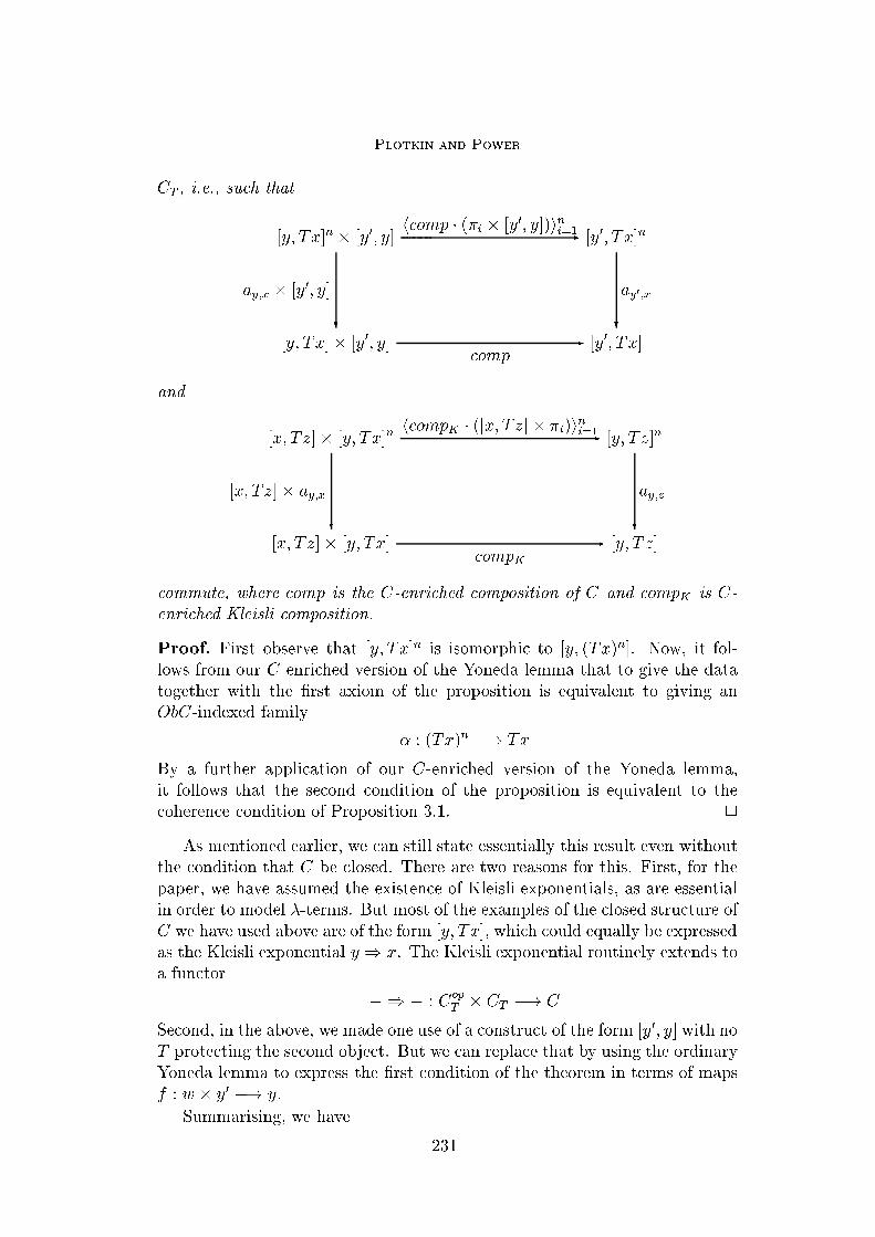
Plotkin and Power

CT , i.e., such that

[y; Tx]n � [y0; y]hcomp � (�i � [y0; y])ini=1

- [y0; Tx]n

[y; Tx]� [y0; y]

ay;x � [y0; y]

?

comp- [y0; Tx]

ay0;x

?

and

[x; Tz]� [y; Tx]nhcompK � ([x; Tz]� �i)i

ni=1- [y; T z]n

[x; Tz]� [y; Tx]

[x; Tz]� ay;x

?

compK

- [y; T z]

ay;z

?

commute, where comp is the C-enriched composition of C and compK is C-

enriched Kleisli composition.

Proof. First observe that [y; Tx]n is isomorphic to [y; (Tx)n]. Now, it fol-lows from our C-enriched version of the Yoneda lemma that to give the data

together with the �rst axiom of the proposition is equivalent to giving anObC-indexed family

� : (Tx)n �! Tx

By a further application of our C-enriched version of the Yoneda lemma,it follows that the second condition of the proposition is equivalent to the

coherence condition of Proposition 3.1. 2

As mentioned earlier, we can still state essentially this result even withoutthe condition that C be closed. There are two reasons for this. First, for the

paper, we have assumed the existence of Kleisli exponentials, as are essentialin order to model �-terms. But most of the examples of the closed structure of

C we have used above are of the form [y; Tx], which could equally be expressed

as the Kleisli exponential y ) x. The Kleisli exponential routinely extends toa functor

� ) � : Cop

T � CT �! C

Second, in the above, we made one use of a construct of the form [y0; y] with no

T protecting the second object. But we can replace that by using the ordinary

Yoneda lemma to express the �rst condition of the theorem in terms of maps

f : w � y0 �! y.

Summarising, we have

231

Plotkin and Power

Corollary 4.2 To give an algebraic operation is equivalent to giving an ObCop�

ObC family of maps

ay;x : (y ) x)n �! (y) x)

in C, such that for every map f : w � y0 �! y in C, the diagram

(y) x)n � w � y0(f ) x)n � w � y0

- ((w � y0)) x)n � w � y0

(y) x)� y

ay;x � f

?

ev- x

ev � (aw�y0;x � w � y0)

?

commutes, and the diagram

(x) z)� (y ) x)nhcompK � ((x) z)� �i)i

ni=1- (y ) z)n

(x) z)� (y ) x)

(x) z)� ay;x

?

compK

- (y) z)

ay;z

?

commutes, where compK is the canonical internalisation of Kleisli composi-

tion.

5 Algebraic operations as generic e�ects

In this section, we apply our formulation of the C-enriched Yoneda lemma to

characterise algebraic operations in entirely di�erent terms again as maps in

CT , i.e., in terms of generic e�ects. Observe that if C has an n-fold coproductn of 1, the functor (T�)n : CT �! C is isomorphic to the functor n ) � :CT �! C. If C is closed, the functor n ) � enriches canonically to a C-

enriched functor, and that C-enriched functor is precisely the representable C-

functor CT (n;�) : CT �! C, where CT is regarded as a C-enriched category.

So by Proposition 3.1 together with our C-enriched version of the Yonedalemma, we immediately have

Theorem 5.1 If C is closed, the C-enriched Yoneda embedding induces a

bijection between maps 1 �! n in CT and algebraic operations

�x : (Tx)n �! Tx

This result is essentially just an instance of an enriched version of theidenti�cation of maps in a Lawvere theory with operations of the Lawvere

theory. Observe that it follows that there is no mathematical reason to restrict

232

Plotkin and Power

attention to algebraic operations of arity n for a natural number n. We could

just as well speak, in this setting, of algebraic operations of the form

�x : (a) �) �! (b) �)

for any objects a and b of C. So for instance, we could include an account

of in�nitary operations as one might use to model operations involved with

state. For speci�c choices of C such as C = Poset, one could consider more

exotic arities such as that given by Sierpinski space.

Once again, by use of parametrisation, we can avoid the closedness as-

sumption on C here, yielding the stronger statement

Theorem 5.2 Functoriality of � ) � : Cop

T � CT �! C in its �rst variable

induces a bijection from the set of maps 1 �! n in CT to the set of algebraic

operations

�x : (Tx)n �! Tx

We regard this as the most profound result of the paper. This result shows

that to give an algebraic operation is equivalent to giving a generic e�ect,i.e., a constant of type the arity of the operation. For example, to give abinary nondeterministic operator for a strong monad T is equivalent to giving

a constant of type 2, and to give equations to accompany the operator isequivalent to giving equations to be satis�ed by the constant. The leading

example here has T being the non-empty �nite powerset monad or a power-domain. Given a nondeterministic operator _, the constant is given by true_false, and given a constant c, the operator is given by M _N = if c then M

else N . There are precisely three non-empty �nite subsets of the two elementset, and accordingly, there are precisely three algebraic operations on the non-

empty �nite powerset monad, and they are given by the two projections and

choice.

The connection of this result with enriched Lawvere theories [12] is as fol-

lows. If C is locally �nitely presentable as a closed category, one can de�ne a

notion of �nitary C-enriched monad on C and a notion of C-enriched Lawvere

theory, and prove that the two are equivalent, generalising the usual equiv-

alence in the case that C = Set. Given a �nitary C-enriched monad T , thecorresponding C-enriched Lawvere theory is given by the full sub-C-category

of CT determined by the �nitely presentable objects. These include all �nite

coproducts of 1. So our results here exactly relate maps in the Lawvere theory

with algebraic operations, generalising Lawvere's original idea. Of course, in

this paper, we do not assume the �niteness assumptions on either the categoryC or the monad T , but our result here is essentially the same.

Theorem 5.2 extends with little fuss to the situation of �nitely presentable

objects a and b; one just requires a suitable re�nement of the construct (T�)n

to account for a and b being objects of C rather than �nite numbers. Thisfollows readily by inspection of the work of [12], and, in a special case, it

seems to provide an account of some of the operations associated with state,

233

Plotkin and Power

as suggested to us by Moggi.

6 Algebraic operations and the category of algebras

Finally, in this section, we characterise the notion of algebraic operation

in terms of the category of algebras T -Alg. The co-Kleisli category of the

comonad on T -Alg induced by the monad T is used to model call-by-name

languages with e�ects, so this formulation gives us an indication of how to

generalise our analysis to call-by-name computation or perhaps to some com-

bination of call-by-value and call-by-name, cf [5].

If C is closed and has equalisers, generalising Lawvere, the results of the

previous section can equally be formulated as equivalences between algebraic

operations and operations

�(A;a) : U(A; a)n �! U(A; a)

natural in (A; a), where U : T -Alg �! C is the C-enriched forgetful functor:

equalisers are needed in C in order to give an enrichment of T -Alg in C.We prove the result by use of our C-enriched version of the Yoneda lemma

again, together with the observation that the canonical C-enriched functorI : CT �! T -Alg is fully faithful. Formally, the result is

Theorem 6.1 If C is closed and has equalisers, the C-enriched Yoneda em-

bedding induces a bijection between maps 1 �! n in CT and C-enriched nat-

ural transformations

� : (U�)n �! U � :

Combining this with Theorem 5.1, we have

Corollary 6.2 If C is closed and has equalisers, to give an algebraic operation

�x : (Tx)n �! Tx

is equivalent to giving a C-enriched natural transformation

� : (U�)n �! U:

One can also give a parametrised version of this result if C is neither closed

nor complete along the lines for CT as in the previous section. It yields

Theorem 6.3 To give an algeberaic operation

�x : (Tx)n �! Tx

is equivalent to giving an Ob(T -Alg)-indexed family of maps

�(A;a) : U(A; a)n �! U(A; a)

such that, for each map

f : x� U(A; a) �! U(B; b)

234

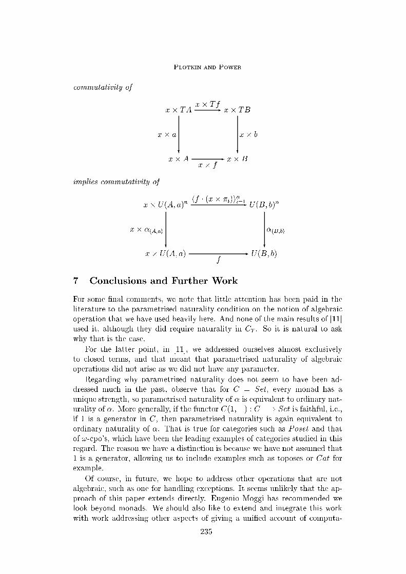
Plotkin and Power

commutativity of

x� TAx� Tf

- x� TB

x� A

x� a

?

x� f- x� B

x� b

?

implies commutativity of

x� U(A; a)nhf � (x� �i)i

ni=1- U(B; b)n

x� U(A; a)

x� �(A;a)

?

f- U(B; b)

�(B;b)

?

7 Conclusions and Further Work

For some �nal comments, we note that little attention has been paid in the

literature to the parametrised naturality condition on the notion of algebraicoperation that we have used heavily here. And none of the main results of [11]used it, although they did require naturality in CT . So it is natural to ask

why that is the case.

For the latter point, in [11], we addressed ourselves almost exclusively

to closed terms, and that meant that parametrised naturality of algebraic

operations did not arise as we did not have any parameter.

Regarding why parametrised naturality does not seem to have been ad-

dressed much in the past, observe that for C = Set, every monad has a

unique strength, so parametrised naturality of � is equivalent to ordinary nat-

urality of �. More generally, if the functor C(1;�) : C �! Set is faithful, i.e.,if 1 is a generator in C, then parametrised naturality is again equivalent to

ordinary naturality of �. That is true for categories such as Poset and that

of !-cpo's, which have been the leading examples of categories studied in this

regard. The reason we have a distinction is because we have not assumed that

1 is a generator, allowing us to include examples such as toposes or Cat forexample.

Of course, in future, we hope to address other operations that are not

algebraic, such as one for handling exceptions. It seems unlikely that the ap-

proach of this paper extends directly. Eugenio Moggi has recommended welook beyond monads. We should also like to extend and integrate this work

with work addressing other aspects of giving a uni�ed account of computa-

235

Plotkin and Power

tional e�ects. We note here especially Paul Levy's work [5] which can be used

to give accounts of both call-by-value and call-by-name in the same setting,

and work on modularity [13], which might also help with other computational

e�ects.

References

[1] Anderson, S.O., and A. J. Power, A Representable Approach to Finite

Nondeterminism, Theoret. Comput. Sci. 177 (1997) 3{25.

[2] Jones, C., \Probabilistic Non-Determinism," Ph.D. Thesis, University of

Edinburgh, Report ECS-LFCS-90-105, 1990.

[3] Jones, C., and G. D. Plotkin, A Probabilistic Powerdomain of Evaluations,

Proc. LICS 4 (1989) 186{195.

[4] Kelly, G.M., \Basic Concepts of Enriched Category Theory," Cambridge:

Cambridge University Press, 1982.

[5] Levy, P.B., Call-by-Push-Value: A Subsuming Paradigm, \Proc. TLCA 99"

Lecture Notes in Computer Science 1581 228{242.

[6] Moggi, E., Computational lambda-calculus and monads, Proc. LICS 89 (1989)

14{23.

[7] Moggi, E., An abstract view of programming languages, University of

Edinburgh, Report ECS-LFCS-90-113, 1989.

[8] Moggi, E., Notions of computation and monads, Inf. and Comp. 93 (1991)

55{92.

[9] Plotkin, G.D., A Powerdomain Construction, SIAM J. Comput. 5 (1976) 452{

487.

[10] Plotkin, G.D., \Domains," (http://www.dcs.ed.ac.uk/home/gdp/), 1983.

[11] Plotkin, G.D., and A. J. Power, Adequacy for Algebraic E�ects, Proc.

FOSSACS 2001 (to appear).

[12] Power, A.J., Enriched Lawvere Theories, Theory and Applications of

Categories (2000) 83{93.

[13] Power, A.J., and E. P. Robinson, Modularity and Dyads, \Proc. MFPS 15"

Electronic Notes in Thoeret. Comp. Sci. 20, 1999.

236

MFPS 17 Preliminary Version

An Algebraic Foundation for Graph-basedDiagrams in Computing

John Power 1,3 and Konstantinos Tourlas 2,4

Division of InformaticsThe University of Edinburgh

Edinburgh EH9 3JZUnited Kingdom

Abstract

We develop an algebraic foundation for some of the graph-based structures underly-ing a variety of popular diagrammatic notations for the specification, modelling andprogramming of computing systems. Using hypergraphs and higraphs as leading ex-amples, a locally ordered category Graph(C) of graphs in a locally ordered categoryC is defined and endowed with symmetric monoidal closed structure. Two other op-erations on higraphs and variants, selected for relevance to computing applications,are generalised in this setting.

1 Introduction

Recent years have witnessed a rapid, ongoing popularisation of diagrammaticnotations in the specification, modelling and programming of computing sys-tems. Most notable among them are Statecharts [4], a notation for modellingreactive systems, and the Unified Modelling Language (UML) [10], a familyof diagrammatic notations for object-based modelling. Invariably, underlyingsuch complex diagrams is some notion of graph, upon which labels and otherlinguistic or visual annotations are added according to application-specificneeds (see e.g. [10,9,3] for a variety of examples).

Beyond ordinary graphs, the two leading examples studied here are hy-pergraphs and higraphs [5]. The latter underlie a number of sophisticateddiagrammatic formalisms including, most prominently, Statecharts, the state

1 This work has been done with the support of EPSRC grant GR/M56333 and a BritishCouncil grant, and the COE budget of STA Japan.2 Support EPSRC grant GR/N12480 and of the COE budget of STA Japan is gratefullyacknowledged.3 Email: ajp@dcs.ed.ac.uk4 Email: kxt@dcs.ed.ac.uk

This is a preliminary version. The final version will be published inElectronic Notes in Theoretical Computer Science

URL: www.elsevier.nl/locate/entcs

Power and Tourlas

diagrams of UML, and the domain-specific language Argos [8] for program-ming reactive systems. Higraphs allow for vitally concise, economical repre-sentations of complex state-transition systems, such as those underlying re-alistic reactive systems, by drastically reducing the number of edges requiredto specify the transition relation. This is achieved by replacing a number oftransitions having, say, a common target state with a single transition havingthe same target but with source a new “super-state” containing all the sourcestates of the original transitions. The resulting reduction in complexity is ofthe order of n2, where n is the number of states.

We begin our analysis by observing that graphs, hypergraphs and higraphsare all instances of the same structure, that of a graph in a category C, with Cbeing respectively Set , Rel and Poset . Other variants are also considered. Thecase of higraphs is motivated and studied extensively and concretely in thedraft paper [13]. The latter assumes only elementary knowledge of categorytheory on the part of the reader, so as to be accessible to a wide audienceof computer scientists who have immediate scientific and practical interestin higraphs and their applications in UML and Statecharts. In the presentpaper, Section 2 introduces our leading examples, followed by a definition inSection 2.4 of a category Graph(C) of graphs in a locally ordered category C.

Underlying Statecharts is a binary operation which given Statecharts Sand S ′ yields a third corresponding to the semantics of S and S ′ operatingconcurrently. We show how the same applies to higraphs and hypergraphs.Here we formulate this precisely and uniformly in algebraic terms by defining asymmetric monoidal closed structure on Graph(C). We do so in Section 3. Itis further shown that symmetric monoidal closed adjunction linking Graph(C)to Cat(C) exists when the latter category bears a generalisation of the “other”symmetric monoidal closed structure on Cat .

Hierarchies of edges in higraphs are exploited in practical applications toproduce concise specifications of complex reactive systems. To understandthe meaning of higher-level edges we introduce in Section 4 a completionoperation on higraphs. This is shown to be an instance of the right adjoint tothe inclusion of Graph(C) into Graphopl(C), the latter having oplax naturaltransformations as arrows. A theorem stating conditions for the existence ofsuch right adjoints is proved.

To support users in working with large, hierarchically structured dia-grams representing complex systems, one requires effective mechanisms forre-organising, abstracting and filtering the information present in diagrams[9]. The leading example studied here is of a filtering operation on higraphs,introduced and motivated by Harel in [5] under the name of zooming out. Weshow in Section 5 how it generalises to graphs in non-trivially locally orderedcategories.

238

Power and Tourlas

Fig. 1. A simple hypergraph.

F

A

B

C D

E

Fig. 2. A simple higraph.

2 Leading examples and main definition

We begin by recalling the standard definition of a (directed, multi-)graph asconsisting of a set V of vertices, a set E of edges and two functions s, t : E −→V giving the source and target of each edge. That is, a graph is a pair ofparallel arrows s, t : E −→ V in the category Set .

2.1 Hypergraphs

Hypergraphs are a generalisation of graphs in which each edge may have setsof vertices as its source and target. The typical pictorial representation of thiskind of directed hypergraph is illustrated in Figure 1.

Thus, a hypergraph consists of a set V of vertices, a set E of edges andtwo functions s, t : E −→ 2V giving sources and targets. Equivalently, s andt may be seen as relations from E to V , thus arriving at the following

Definition 2.1 A hypergraph is a pair of parallel maps in the category Rel of(small) sets and relations.

2.2 Higraphs

Higraph is a term coined-up by Harel[5] as short for hierarchical graph, butis often used to include several variants. The definitive feature of higraphs,common to all variants, is referred to as depth, meaning that nodes may becontained inside other nodes. Figure 2 illustrates the standard pictorial rep-resentation of a higraph consisting of six nodes and four edges, with the nodeslabelled B, C and D being spatially contained within the node labelled A. Itis therefore common, and we shall hereafter adhere to convention, to call thenodes of a higraph blobs, as an indication of their pictorial representation by

239

Power and Tourlas

convex contours on the plane. For further details the reader is referred to [13].

The containment relation on blobs is captured by requiring poset struc-ture on the set of blobs. The notion of higraph developed here extends thisrequirement to the set of edges:

Definition 2.2 A higraph is a pair of parallel arrows s, t : E −→ B in thecategory Poset.

In practice, a higraph typically arises as a graph (B,E, s, t) together witha partial order ≤B on B. In that case, the poset structure on E may be takento be the discrete one. However, other choices of orders on E are often useful,e.g. for encoding the conflict resolution schemes [6] adopted in Statecharts.

In most applications of higraphs, especially Statecharts, the intuitive un-derstanding of en edge e is as implying the presence of “lower-level”, implicitedges from all blobs contained in s(e) to all blobs contained in t(e). The pointin general is that a multitude of edges is made implicit in a single, explicitlyshown higher-level edge. In Statecharts, this device is employed for repre-senting interrupt transitions, thus drastically reducing the number of edgesrequired to specify the transition relation among the states of the representedtransition system.

2.3 Combinations and variants

To deal with realistic diagrams, one may additionally wish to combine featuresfound in different notions of graph, e.g. to allow edges in higraphs to havemultiple sources and targets, as is indeed allowed in some Statecharts. Theresulting notion of graph, a combination of simple higraphs (as defined above)and hypergraphs, could be approached by considering the category of posetsand relations between their underlying sets. The category BSup of posets withall binary sups (and sup-preserving monotone maps) gives a better model ofdepth in Statecharts. One may also consider graphs in the category ω-Cpo ofω-complete partial orders.

2.4 Graphs in locally ordered categories

Each of our leading examples of “notions of graph” has been cast in terms of apair of parallel maps in a suitable category C. Another, less obvious common-ality among our examples is that C has been a locally ordered category, i.e.a category enriched in the cartesian closed category Poset of posets, a fact ofwhich substantial use will be made later. (The category Set is locally orderedin a trivial sense: each hom-object is a discrete poset.) Generalising from oursituation one has:

Definition 2.3 Let C be a locally ordered category. Let Graph(C) denote thelocally ordered category of graphs in C, that is the functor category [·→→ ·, C]where the category ·→→ · consists of two objects and two non-identity maps asshown. 2

240

Power and Tourlas

h

B

C

D

E

F

G

j f

e

k

g

A

Fig. 3. A simple Statechart

f

B

C

j ⊗ h

F

G e

k

g E=

B,E

B,F

C,G

C,E

B,G

C,F

k h

f j

k

f j j f

eg

h

g

e

Fig. 4. Operation underlying the Statechart of Fig. 3

So, an object of Graph(C) consists of a pair of objects E and V of C,together with a pair of maps s, t : E −→ V in C. An arrow of Graph(C)from (E, V, s, t : E −→ V ) to (E ′, V ′, s′, t′ : E ′ −→ V ′) consists of mapsfE : E −→ E ′ and fV : V −→ V ′ such that fV s = s′fE and fV t = t′fE. Thelocal order of Graph(C) is generated by that of C, i.e., (fE, fV ) ≤ (gE, gV ) iffE ≤ gE and fV ≤ gV .

3 A symmetric monoidal closed structure on Graph(C)

We now proceed to study some extra structure on Graph(C), for well-behavedC. Our motivation arises from the application of higraphs in Statecharts.Specifications of complex reactive systems directly in terms of transition sys-tems become impractical to visualise owing to the large number of statesinvolved. Statecharts deal with this problem by allowing the modelling ofreactive systems directly in terms of their identifiable concurrent subsystems:

Example 3.1 Consider the Statechart in Figure 3 representing two subsys-tems A and D operating concurrently. Assuming an interleaving model ofconcurrency, as is the case with Statecharts, the meaning of this picture iscaptured precisely by the operation where the resulting transition system isexactly the intended behaviour of the complete system. 2

A consequence of our results in this section is that the above operation,which in [5] is referred to as “a sort of product of automata”, generalises

241

Power and Tourlas

smoothly to higraphs. This is an essential step in pinpointing the precisemathematical structures underpinning the semantics of Statecharts. For, moregenerally, the specifications of the subsystems A and D in Figure 3 typicallybear higraph structure.

So for our next main result, we observe that, generalising the situation forC = Set in Example 3.1, here not requiring local order structure on C, wehave

Theorem 3.2 For any cartesian closed category C with finite coproducts, thecategory Graph(C) has a symmetric monoidal structure given as follows: givenG = (E, V, s, t) and G′ = (E ′, V ′, s′, t′), the graph G ⊗ G′ has vertex objectV × V ′ and edge object (E × V ′) + (V × E ′), with source and target mapsevident. The unit of this symmetric monoidal structure is given by V = 1 andE = 0.

Proof. That ⊗ is a bifunctor follows directly from the properties of the binaryproducts and coproducts in C. The required isomorphisms are easily deducedfrom those associated with the symmetric monoidal structure induced on Cby its cartesian structure, and the verification of the required coherence con-ditions is routine. 2

Example 3.3 On higraphs ⊗ yields a straightforward generalisation of theoperation in Figure 4. Specifically χ⊗χ′ contains an edge 〈b1, b

′〉 → 〈b2, b′〉 for

every edge b1 → b2 in χ and blob b′ in χ′, and an edge 〈b, b′1〉 → 〈b, b′2〉 for everyedge b′1 → b′2 in χ′ and blob b in χ. Containment is given by 〈b1, b

′1〉 ≤ 〈b2, b

′2〉

iff b1 ≤ b2 and b′1 ≤ b′2. In the case of hypergraphs, H ⊗ H ′ contains an edge{〈x1, x

′〉, . . . , 〈xn, x′〉} → {〈y1, x

′〉, . . . , 〈ym, x′〉} for each edge {x1, . . . , xn} →{y1, . . . , ym} in H and vertex x′ in χ′, and similarly for the edges in H ′.

Theorem 3.4 For any cartesian closed category C with finite coproducts andfinite limits, the symmetric monoidal structure on Graph(C) given in Theo-rem 3.2 is closed.

Proof. The exponential object [G′, G′′] has object of vertices the domain ofthe equaliser of the two maps from [V ′, V ′′]×[E ′, E ′′] to [E ′, V ′] × [E ′, V ′] givenby 〈[s′, V ′], [t′, V ′]〉◦π0 and 〈[E ′, s′], [E ′, t′]〉◦π1 where π0, π1 are the projectionsfrom [V ′, V ′′] × [E ′, E ′′]. The object of edges of [G′, G′′] is the domain of theequaliser of the maps 〈π0 ◦ q ◦ π′

0, π0 ◦ q ◦ π′2〉 and 〈[V ′, s′′] ◦ π′

1, [V ′, t′′] ◦ π′1〉,

both having domain V × [V ′, E ′′] × V and codomain [V ′, V ′′] × [V ′, V ′′], whereπ′

i are the three projections out of V × [V ′, E ′′] × V . 2

Notice, in particular, that the exponential in the category Graph(C) with thetensor product defined in the theorem is particularly natural. The object ofvertices represents all graph homomorphisms from G to G′, and the object ofedges represents all transformations between graph homomorphisms.

242

Power and Tourlas

3.1 A symmetric monoidal closed adjunction

It is well known that one may define categories in any category C with finitelimits, the usual category Cat being isomorphic to the category of modelsCat(Set) in Set of an appropriate finite limit sketch [1]. We shall write Cat(C)for the category of categories in C, implicitly asserting C to have finite limitsas required.

While it is well known that Cat is a cartesian closed category, it is farless well known that there is precisely one other symmetric monoidal closedstructure on Cat [2,12]. We refer to the other one as the other symmetricmonoidal closed structure on Cat, which may be outlined as follows:

• The exponential A −→ B is given by the set of functors from A to B, witha morphism from g to h being the assignment of an arrow αx : gx −→ hxto each object x of A. The composition is obvious. We shall call an arrowof A −→ B a transformation.

• The tensor product may be described in terms of a universal property: itis the universal D for which one has, for each object x of A, a functorhx : B −→ D and for each object y of B, a functor ky : A −→ D suchthat hxy = kyx for each (x, y). The unit of the tensor product is the unitcategory.

Explicitly, the tensor product A ⊗ B of A and B has as object set ObA ×ObB, and an arrow from (x, y) to (x′, y′) consists of a finite sequence of non-identity arrows, with alternate arrows forming a directed path in A, and theothers forming a directed path in B. Composition is given by concatenation,then cancellation accorded by the composition of A and B. The symmetry isobvious.

It is routine to verify that if, in addition to having finite limits, C is co-complete and cartesian closed, the other symmetric monoidal closed structureextends to Cat(C). We are now in position to state our theorem relatingCat(C) to Graph(C):

Theorem 3.5 For a cocomplete cartesian closed category C with finite lim-its, the forgetful functor U : Cat(C) −→ Graph(C) is part of a symmetricmonoidal closed adjunction with respect to the other tensor product on Cat(C)and the above symmetric monoidal closed structure on Graph(C).

Proof. For a proof, consider the case that C is Set and simply internalise theargument there. 2

Note that a corresponding result does not hold for the cartesian closedstructures of Cat(C) and Graph(C) even in the case of C = Set, so we regardthis result as strong evidence of the naturalness of this structure. Finally, inthis vein, we observe

Theorem 3.6 For cartesian closed C with finite coproducts, the forgetfulfunctor from Graph(C) to C is part of a symmetric monoidal closed adjunc-

243

Power and Tourlas

Fig. 5. Completion of a simple higraph, where the added edges are shown dashed.

tion with respect to the above symmetric monoidal structure on Graph(C).

Proof. For a proof, consider the proof in the case of C = Set and routinelyinternalise it to C. 2

Again, even in the case of C = Set, a corresponding result does not hold inrespect of the cartesian closed structure of Graph(C) as the left adjoint doesnot preserve the unit, i.e., it does not send 1 to the terminal object of Graphas the latter has an edge.

4 A completion operation

A construction useful in understanding the semantics of higraphs and variants(for instance that involving the categories BSup or ω-Cpo) is to explicate alledges which are understood as being implicitly present in a higraph (recallthe discussion near the end of Section 2.2). This “completion” operation isillustrated in Figure 5.

Definition 4.1 Let χ = s, t : E −→ B be a higraph. The higraph T (χ), calledthe completion of χ, has blobs B and edges the subset of E×(B×B) consistingof those pairs 〈e, 〈b, b′〉〉 such that b ≤B s(e) and b′ ≤B t(e), partially orderedpointwise, with source and target given by projections. 2

Definition 4.2 Given a locally ordered category C, we denote by Graphopl(C)the locally ordered category whose objects are graphs in C and whose arrowsare oplax transformations, i.e. pairs (fE : E −→ E ′, fV : V −→ V ′) such thatfV s ≤ s′fE and fV t ≤ t′fE, with local order structure induced by that of C. 2

To state our theorem, it is convenient to use a little of the theory of 2-categories, specifically some finite limits. A convenient account of such limitsis [7]. In particular, we need to use the notion of an oplax limit of a map. Sowe recall it here.

Definition 4.3 Given an arrow f : X −→ Y in a locally ordered category C,

244

Power and Tourlas

an oplax limit of f is given by a diagram of the form

Lπo - X

≤

L

id

?

π1

- Y

f

?

satisfying two properties:

• for any other diagram of the form

Kh0 - X

≤

K

id

?

h1

- Y

f

?

there is a unique arrow u : K −→ L such that π0u = h0 and π1u = h1, and

• (the two-dimensional property) for any two diagrams of the form

Kh0 - X K

h′0 - X

≤ ≤

K

id

?

h1

- Y

f

?K

id

?

h′1

- Y

f

?

with h0 ≤ h′0 and h1 ≤ h

′1, it follows that u ≤ u′.

2

Theorem 4.4 If the locally ordered category C has finite limits, then the in-clusion of Graph(C) into Graphopl(C) has a right adjoint.

Proof. Given a graph G = (E, V, s, t), the right adjoint has vertex objectgiven by V and object of edges given by the oplax limit of the map 〈s, t〉 :E −→ V × V . It is a routine exercise in 2-categories to prove that thisconstruction yields a right adjoint. 2

The 2-category theory expert will observe that we have only used pie-limitsin C, which may become important in due course [11]. Perhaps a more familiarexpression for the oplax limit used in the proof is in terms of a comma objectin C from the identity map on V × V to the map 〈s, t〉 : E −→ V × V . If

245

Power and Tourlas

F

A

B

C D

E

F

A

E

Fig. 6. Zooming out of a blob in a higraph

C were the locally ordered category Poset, then the right adjoint could bedescribed explicitly by placing an edge from v to v′ if there is an edge from avertex greater than or equal to v to a vertex greater than or equal to v′ in G.This matches exactly our explicit description of T in Definition 4.1.

Dually, if C has finite colimits, the inclusion of Graph(C) into Graphopl(C)has a left adjoint.

5 Zooming out

We begin by recalling Harel’s simple instance of a zooming operation on hi-graphs: the selection of a single blob and the subsequent removal from viewof all blobs contained in it. An example is illustrated in the transition fromthe left to the right half of Figure 6.

To capture the notion of selecting a blob in a higraph we need the following:

Definition 5.1 A pointed higraph ψ consists of an ordinary higraph χ =s, t : E −→ B together with a distinguished blob, given as a map 1 −→ Bin Poset and called the point of ψ. The category H? has pointed higraphsas its objects and maps those ones which preserve points. Let H?,min be thefull subcategory of H? consisting of all objects (pointed higraphs) in which thepoint is minimal wrt. the partial order on blobs; in other words, the point isan atomic blob. Let I be the full functor including H?,min into H?. 2

Consider a pointed higraph ψ with χ = (s, t : E −→ B) and point, say,p ∈ B. The pointed higraph Z(ψ), obtained by zooming out of the point inψ, is determined by the following data:

• blobs: B′ = B \ {b | b < p} (ordered by the restriction to B′ of the partialorder on B);

• edges: E, with the source and target functions being q ◦ s and q ◦ t respec-tively, where q : B −→ B′ is the (obviously monotone) function mappingeach b 6< p in B to b ∈ B′ and each b < p to p ∈ B′;

• point: p

One now has the following [13]:

Proposition 5.2 The function Z extends to a functor from H? to H?,min

which is left adjoint to the inclusion functor I. 2

This proposition will be shown an instance of Theorem 5.5 below. Gener-

246

Power and Tourlas

alising the essential structure underlying our leading example one has:

Definition 5.3 Given a locally ordered category C, denote by Graph(C)∗ thelocally ordered category for which an object consists of a graph (E, V, s, t) inC together with a map v : 1 −→ V in C. The maps are pairs of maps thatstrictly preserve the structure. 2

Definition 5.4 Given a locally ordered category C, denote by Graph(C)∗min

the locally ordered full subcategory of Graph(C)∗ such that the point v : 1 −→V is a minimal element in the poset C(1, V ). 2

Theorem 5.5 If C is a cocomplete locally ordered category, then the inclusionof Graph(C)∗min in Graph(C)∗ has a left adjoint.

Proof. Given (E, V, s, t) and v : 1 −→ V , take the joint coequaliser of v withall of the elements of the poset C(1, V ) that are less than or equal to it. It isroutine to verify that this gives the left adjoint. 2

Example 5.6 For graphs in BSup the theorem gives the expected generali-sation of the zoom-out operation on graphs in Poset in the presence of theextra structure given by binary sups. However, zoom-outs do not generalise tographs in Rel , or the category of posets and relations between their underlyingsets, as the terminal object is the empty set (poset).

6 Further work

Our aim is to develop, in an incremental and principled way, structures whichbear sufficient detail to model realistic diagrammatic notations. Currently weare working towards providing such a model for a large class of Statecharts,which include features found in higraphs and hypergraphs. The work hereinpresented lays the abstract foundations for our approach, in which notions ofgraph and combinations thereof may be studied.

Another strand of our work is to study extensions to such notions of graph,as required to support users in performing specification and reasoning taskswith diagrams. For instance, a mild extension to higraphs was briefly intro-duced by Harel in [5], permitting edges to be “loosely” attached to nodes, thefour possibilities being illustrated in

A

BE

F

.

The rationale was to indicate transitions or relations between some as yetunspecified, or purposefully omitted (e.g. as the result of zooming out) partsof the represented system. For motivation and details the reader is referredto [13]. We conclude by noting that such graphs with “loose edges” can beadded easily to our framework, provided that the locally ordered category C

247

Power and Tourlas

has finite (pie) colimits, thereby allowing one to define tensors with the arrowposet.

References

[1] M. Barr and C. Wells. Category Theory for Computing Science. Prentice-Hall,1990.

[2] F. Foltz, C.M. Kelly, and C. Lair. Algebraic categories with few monoidalbiclosed structures or none. Journal of Pure and Applied Algebra, 17:171–177,1980.

[3] Corin Gurr and Konstantinos Tourlas. Towards the principled design ofsoftware engineering diagrams. In Proceedings of the 22nd InternationalConference on Software Engineering, pages 509–520. ACM, IEEE ComputerSociety, ACM Press, 2000.

[4] David Harel. Statecharts: A visual approach to complex systems. Science ofComputer Programming, 8(3):231–275, 1987.

[5] David Harel. On visual formalisms. Communications of the ACM, 31(5):514–530, 1988.

[6] David Harel and Amnon Naamad. The STATEMATE semantics of Statecharts.ACM Transactions on Software Engineering Methodology, 5(4), October 1996.

[7] G.M. Kelly. Elementary observations on 2-categorical limits. Bull. Austral.Math. Soc., pages 301–317, 1989.

[8] F. Maraninchi. The Argos language: Graphical representation of automata anddescription of reactive systems. In Proceedings of the IEEE Workshop on VisualLanguages, 1991.

[9] Bonnie M. Nardi. A Small Matter of Programming: Perspectives on End-UserComputing. MIT Press, 1993.

[10] Rob Pooley and Perdita Stevens. Using UML. Addison Wesley, 1999.

[11] A.J. Power and E.P. Robinson. A characterization of pie-limits. Math. Proc.Cambridge Philos. Soc., 110:33–47, 1991.

[12] John Power and Edmund Robinson. Premonoidal categories and notions ofcomputation. Mathematical Structures in Comp. Science, 11, 1993.

[13] John Power and Konstantinos Tourlas. An algebraic foundation for higraphs.Submitted for publication, March 2001.

248

MFPS 17 Preliminary Version

Comparing Control Constructs byDouble-barrelled CPS Transforms

Hayo Thielecke

H.Thielecke@cs.bham.ac.ukSchool of Computer ScienceUniversity of Birmingham

BirminghamUnited Kingdom

Abstract

We investigate continuation-passing style transforms that pass two continuations.Altering a single variable in the translation of λ-abstraction gives rise to differentcontrol operators: first-class continuations; dynamic control; and (depending ona further choice of a variable) either the return statement of C; or Landin’s J-operator. In each case there is an associated simple typing. For those constructsthat allow upward continuations, the typing is classical, for the others it remainsintuitionistic, giving a clean distinction independent of syntactic details.

1 Introduction

Control operators come in bewildering variety. Sometimes the same termis used for distinct constructs, as with catch in early Scheme or throw inStandard ML of New Jersey, which are very unlike the catch and throw

in Lisp whose names they borrow. On the other hand, this Lisp catch isfundamentally similar to exceptions despite their dissimilar and much moreornate appearance.

Fortunately it is sometimes possible to glean some high-level “logical” viewof a programming language construct by looking only at its type. Specificallyfor control operations, Griffin’s discovery [3] that call/cc and related op-erators can be ascribed classical types gives us the fundamental distinctionbetween languages that have such classical types and those that do not, eventhough they may still enjoy some form of control. This approach complementscomparisons based on contextual equivalences [10,14].

Such a comparison would be difficult unless we blot out complication.In particular, exceptions are typically tied in with other, fairly complicatedfeatures of the language which are not relevant to control as such: in ml

with the datatype mechanism, in Java with object-orientation. In order toThis is a preliminary version. The final version will be published in

Electronic Notes in Theoretical Computer ScienceURL: www.elsevier.nl/locate/entcs

Thielecke

simplify, we first strip down control operators to the bare essentials of labellingand jumping, so that there are no longer any distracting syntactic differencesbetween them. The grammar of our toy language is uniformly this:

M ::= x | λx.M | MM | hereM | goM.

The intended meaning of here is that it labels a “program point” or expressionwithout actually naming any particular label—just uttering the demonstrative“here”, as it were. Correspondingly, go jumps to a place specified by a here,without naming the “to” of a goto.

Despite the simplicity of the language, there is still scope for variation:not by adding bells and whistles to here and go, but by varying the meaningof λ-abstraction. Its impact can be seen quite clearly in the distinction be-tween exceptions and first-class continuations. The difference between themis as much due to the meaning of λ-abstraction as due to the control operatorsthemselves, since λ-abstraction determines what is statically put into a closureand what is passed dynamically. Readers familiar with, say, Scheme imple-mentations will perhaps not be surprised about the impact of what becomespart of a closure. But the point of this paper is twofold:

• small variations in the meaning of λ completely change the meaning of ourcontrol operators;

• we can see these differences at an abstract, logical level, without delvinginto the innards of interpreters.

We give meaning to the λ-calculus enriched with here and go by meansof continuations in Section 2, examining in Sections 3–5 how variations on λ-abstraction determine what kind of control operations here and go represent.For each of these variations we present a simple typing, which agrees with thetransform (Section 6). We conclude by explaining the significance of thesetypings in terms of classical and intuitionistic logic (Section 7).

2 Double-barrelled CPS

Our starting point is a continuation-passing style (cps) transform. This trans-form is double-barrelled in the sense that it always passes two continuations.Hence the clauses start with λkq. . . . instead of λk. . . .. Other than that, thiscps transform is in fact a very mild variation on the usual call-by-value one [8].As indicated by the ? , we leave one variable, the extra continuation passedto the body of a λ-abstraction, unspecified.

[[x]] = λkq.kx

[[λ?x.M ]] = λks.k(λxrd.[[M ]]r ? )

[[MN ]] = λkq.[[M ]](λm.[[N ]](λn.mnkq)q)q

[[hereM ]] = λkq.[[M ]]kk

[[goM ]] = λkq.[[M ]]qq

The extra continuation may be seen as a jump continuation, in that its

250

Thielecke

manipulation accounts for the labelling and jumping. This is done symmet-rically: here makes the jump continuation the same as the current one k,whereas go sets the current continuation of its argument to the jump contin-uation q. The clauses for variables and applications do not interact with theadditional jump continuation: the former ignores it, while the latter merelydistributes it into the operator, the operand and the function call.

Only in the clause for λ-abstraction do we face a design decision. Depend-ing on which continuation (static s, dynamic d, or the return continuationr) we fill in for “?” in the clause for λ, there are three different flavours ofλ-abstraction.

[[λsx.M ]] = λks.k(λxrd.[[M ]]r s )

[[λdx.M ]] = λks.k(λxrd.[[M ]]r d )

[[λrx.M ]] = λks.k(λxrd.[[M ]]r r )

The lambdas are subscripted to distinguish them, and the box around the lastvariable is meant to highlight that this is the crucial difference between thetransforms. Formally there is also a fourth possibility, the outer continuationk, but this seems less meaningful and would not fit into simple typing.

For all choices of λ, the operation go is always a jump to a place specifiedby a here. For example, for any M , the term here ((λx.M)(goN)) should beequivalent to N , as the go jumps past the M . But in more involved examplesthan this, there may be different choices where go can go to among severaloccurrences of here. In particular, if s is passed as the second continuationargument to M in the transform of λx.M , then a go in M will refer to thehere that was in scope at the point of definition (unless there is an interveninghere, just as one binding of a variable x can shadow another). By contrast,if d is passed to M in λx.M , then the here that is in scope at the point ofdefinition is forgotten; instead go in M will refer to the here that is in scopeat the point of call when λx.M is applied to an argument. In fact, dependingupon the choice of variable in the clause for λ as above, here and go give riseto different control operations:

• first-class continuations like those given by call/cc in Scheme [4];

• dynamic control in the sense of Lisp, and typeable in a way reminiscent ofchecked exceptions;

• a return-operation, which can be refined into the J-operator invented byLandin in 1965 and ancestral to call/cc [4,6,7,13].

We examine these constructs in turn, giving a simple type system in eachcase. An unusual feature of these type judgements is that, because we havetwo continuations, there are two types in the succedent on the right of theturnstile, as in

Γ ` M : A,B.

The first type on the right accounts for the case that the term returns a value;it corresponds to the current continuation. The second type accounts for the

251

Thielecke

Fig. 1. Typing for static here and go

Γ, x : A, Γ′ `s x : A,C

Γ `s M : B,B

Γ `s hereM : B,C

Γ `s M : B,B

Γ `s goM : C,B

Γ, x : A `s M : B,C

Γ `s λsx.M : A → B,C

Γ `s M : A → B,C Γ `s N : A,C

Γ `s MN : B,C

jump continuation. In logical terms, the comma on the right may be read asa disjunction. It makes a big difference whether this disjunction is classicalor intuitionistic. That is our main criterion of comparing and contrasting thecontrol constructs.

3 First-class continuations

The first choice of which continuation to pass to the body of a function isarguably the cleanest. Passing the static continuation s gives control thesame static binding as ordinary λ-calculus variables. In the static case, thetransform is this:

[[x]] = λkq.kx

[[λsx.M ]] = λks.k(λxrd.[[M ]]r s )

[[MN ]] = λkq.[[M ]](λm.[[N ]](λn.mnkq)q)q

[[hereM ]] = λkq.[[M ]]kk

[[goM ]] = λkq.[[M ]]qq

We type our source language with here and go as in Figure 1.

In logical terms, both here and go are a combined right weakening andcontraction. By themselves, weakening and contraction do not amount tomuch; but it is the combination with the rule for →-introduction that makesthe calculus “classical”, in the sense that there are terms whose types arepropositions of classical, but not of intuitionistic, minimal logic.

To see how →-introduction gives classical types, consider λ-abstractingover go.

x : A `s gox : B,A

`s λsx.gox : A → B,A

If we read the comma as “or”, and A→B for arbitrary B as “not A”, thenthis judgement asserts the classical excluded middle, “not A or A”. We buildon the classical type of λsx.gox for another canonical example: Scheme’s

252

Thielecke

call-with-current-continuation (call/cc for short) operator [4]. It issyntactic sugar in terms of static here and go:

call/cc = λsf.(here (f (λsx.gox))).

As one would expect [3], the type of call/cc is Peirce’s law “if not A impliesA, then A”. We derive the judgement

`s λsf.(here (f (λsx.gox))) : ((A → B) → A) → A,C

as follows. Let Γ be the context f : (A → B) → A. Then we derive:

Γ `s f : (A → B) → A,A

Γ, x : A `s x : A,A

Γ, x : A `s gox : B,A

Γ `s λsx.gox : A → B,A

Γ `s (f (λsx.gox)) : A,A

Γ `s here (f (λsx.gox)) : A,C

`s λsf.(here (f (λsx.gox))) : ((A → B) → A) → A,C

As another example, let Γ be any context, and assume we have Γ `s M : A,B.Right exchange is admissible in that we can also derive Γ `s M ′ : B,A forsome M ′.

In the typing of call/cc, a go is (at least potentially, depending on f)exported from its enclosing here. Conversely, in the derivation of right ex-change, a go is imported into a here from without. What makes everythingwork is static binding.

4 Dynamic control

Next we consider the dynamic version of here and go. The word “dynamic”is used here in the sense of dynamic binding and dynamic control in Lisp.Another way of phrasing it is that with a dynamic semantics, the here thatis in scope at the point where a function is called will be used, as opposed tothe here that was in scope at the point where the function was defined—thelatter being used for the static semantics.

In the dynamic case, the transform is this:

[[x]] = λkq.kx

[[λdx.M ]] = λks.k(λxrd.[[M ]]r d )

[[MN ]] = λkq.[[M ]](λm.[[N ]](λn.mnkq)q)q

[[hereM ]] = λkq.[[M ]]kk

[[goM ]] = λkq.[[M ]]qq

In this transform, the jump continuation acts as a handler continuation; sinceit is passed as an extra argument on each call, the dynamically enclosinghandler is chosen. Hence under the dynamic semantics, here and go becomea stripped-down version of Lisp’s catch and throw with only a single catch

253

Thielecke

Fig. 2. Typing for dynamic here and go

Γ, x : A, Γ′ `d x : A,C

Γ `d M : B,B

Γ `d hereM : B,C

Γ `d M : B,B

Γ `d goM : C,B

Γ, x : A `d M : B,C

Γ `d λdx.M : A → B ∨ C,D

Γ `d M : A → B ∨ C,C Γ `d N : A,C

Γ `d MN : B,C

tag. These catch and throw operation are themselves a no-frills version ofexceptions with only identity handlers. We can think of here and go as aspecial case of these more elaborate constructs:

hereM ≡ (catch ’e M)

goM ≡ (throw ’e M)

Because the additional continuation is administered dynamically, we can-not fit it into our simple typing without annotating the function type. So fordynamic control, we write the function type as A→B ∨C. Syntactically, thisshould be read as a single operator with the three arguments in mixfix. Weregard the type system as a variant of intuitionistic logic in which → and ∨always have to be introduced or eliminated together.

This annotated arrow can be seen as an idealization of the Java throws

clause in method definitions, in that A → B ∨ C could be written as

B(A) throws C

in a more Java-like syntax. A function of type A → B ∨ C may throw thingsof type C, so it may only be called inside a here with the same type. Ourtyping for the language with dynamic here and go is presented in Figure 2.

We do not attempt to idealize the ML way of typing exceptions becauseML uses a universal type exn for exceptions, in effect allowing a carefullydelimited area of untypedness into the language. The typing of ML exceptionsis therefore much less informative than that of checked exceptions.

Note that here and go are still the same weakening and contraction hybridas in the static setting. But here their significance is a completely different onebecause the →-introduction is coupled with a sort of ∨-introduction. To seethe difference, recall that in the static setting λ-abstracting over a go reifiesthe jump continuation and thereby, at the type level, gives rise to classicaldisjunction. This is not possible with the version of λ that gives go thedynamic semantics. Consider the following inference:

x : A `d gox : B,A

`d λdx.gox : A → B ∨ A,C

254

Thielecke

The C-accepting continuation at the point of definition is not accessible to thego inside the λd. Instead, the go refers only to the A-accepting continuationthat will be available at the point of call. Far from the excluded middle, thetype of λdx.gox is thus “A implies A or B; or anything”.

In the same vein, as a further illustration how fundamentally different thedynamic here and go are from the static variety, we revisit the term that, inthe static setting, gave rise to call/cc with its classical type:

λf.here (f (λx.gox)).

Now in the dynamic case, we can only derive the intuitionistic formula

((A → B ∨ A) → A ∨ A) → A ∨ C

as the type of this term.

Let Γ be the context f : (A → B ∨ A) → A ∨ A. Then we have:

Γ `d f : (A → B ∨ A) → A ∨ A,A

Γ, x : A `d x : A,A

Γ, x : A `d gox : B,A

Γ `d λdx.gox : A → B ∨ A,A

Γ `d (f (λdx.gox)) : A,A

Γ `d here (f (λdx.gox)) : A,C

`d λdf.here (f (λdx.gox)) : ((A → B ∨ A) → A ∨ A) → A ∨ C,D

5 Return continuation

Our last choice is passing the return continuation as the extra continuation tothe body of a λ-abstraction. So the cps transform is this:

[[x]] = λkq.qx

[[λrx.M ]] = λks.k(λxrd.[[M ]]r r )

[[MN ]] = λkq.[[M ]](λm.[[N ]](λn.mnkq)q)q

[[hereM ]] = λkq.[[M ]]kk

[[goM ]] = λkq.[[M ]]qq

This transform grants λr the additional role of a continuation binder. Theoriginal operator for this purpose, here, is rendered redundant, since hereMis now equivalent to (λrx.M)(λry.y) where x is not free in M . At first sight,binding continuations seems an unusual job for a λ; but it becomes less so ifwe think of go as the return statement of C or Java.

5.1 Non-first class return

Because the enclosing λ determines which continuation go jumps to with itsargument, the go-operator has the same effect as a return statement. The

255

Thielecke

Fig. 3. Typing for go as a return-operation

Γ, x : A, Γ′ `r x : A,C

Γ `r M : B,B

Γ `r goM : C,B

Γ, x : A `r M : B,B

Γ `r λrx.M : A → B,C

Γ `r M : A → B,C Γ `r N : A,C

Γ `r MN : B,C

type of extra continuation assumed by go needs to agree with the return typeof the nearest enclosing λ:

Γ, x : A `r M : B,B

Γ `r λrx.M : A → B,C

The whole type system for the calculus with λr is in Figure 3.

The agreement between go and the enclosing λr is comparable with thetyping in C, where the expression featuring in a return statement must havethe return type declared by the enclosing function. For instance, M needs tohave type int in the definition:

int f(){ . . . return M; . . . }

With λr, the special form go cannot be made into a first-class function. Ifwe try to λ-abstract over gox by writing λrx.gox then go will refer to thatλr.

The failure of λr to give first-class returning can be seen logically as follows.In order for λr to be introduced, both types on the right have to be the same:

x : A `r gox : A,A

`r λrx.gox : A → A,C

Rather than the classical “not A or A” this asserts merely the intuitionistic“A implies A; or anything”.

One has a similar situation in Gnu C, which has both the return statementand nested functions, without the ability to refer to the return address ofanother function. If we admit go as a first-class function, it becomes a muchmore powerful form of control, Landin’s JI-operator.

5.2 The JI-operator

Keeping the meaning of λr as a continuation binder, we now consider a controloperator JI that always refers to the statically enclosing λr, but which, unlikethe special form go, is a first-class expression, so that we can pass the returncontinuation to some other function f by writing f(JI). The cps of thisoperator is this:

[[JI]] = λks.k(λxrd. s x)

That is almost, but not quite, the same as if we tried to define JI as λrx.gox:

256

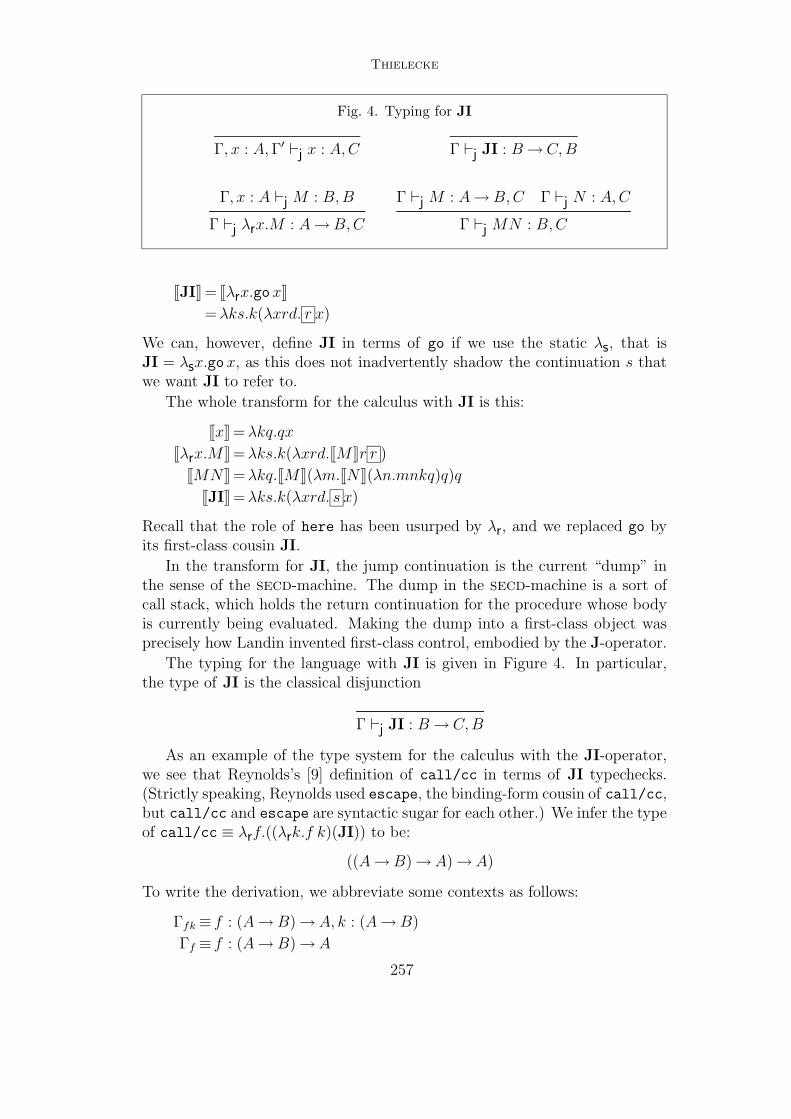
Thielecke

Fig. 4. Typing for JI

Γ, x : A, Γ′j x : A,C Γ j JI : B → C,B

Γ, x : A j M : B,B

Γ j λrx.M : A → B,C

Γ j M : A → B,C Γ j N : A,C

Γ j MN : B,C

[[JI]] = [[λrx.gox]]

= λks.k(λxrd. r x)

We can, however, define JI in terms of go if we use the static λs, that isJI = λsx.gox, as this does not inadvertently shadow the continuation s thatwe want JI to refer to.

The whole transform for the calculus with JI is this:

[[x]] = λkq.qx

[[λrx.M ]] = λks.k(λxrd.[[M ]]r r )

[[MN ]] = λkq.[[M ]](λm.[[N ]](λn.mnkq)q)q

[[JI]] = λks.k(λxrd. s x)

Recall that the role of here has been usurped by λr, and we replaced go byits first-class cousin JI.

In the transform for JI, the jump continuation is the current “dump” inthe sense of the secd-machine. The dump in the secd-machine is a sort ofcall stack, which holds the return continuation for the procedure whose bodyis currently being evaluated. Making the dump into a first-class object wasprecisely how Landin invented first-class control, embodied by the J-operator.

The typing for the language with JI is given in Figure 4. In particular,the type of JI is the classical disjunction

Γ j JI : B → C,B

As an example of the type system for the calculus with the JI-operator,we see that Reynolds’s [9] definition of call/cc in terms of JI typechecks.(Strictly speaking, Reynolds used escape, the binding-form cousin of call/cc,but call/cc and escape are syntactic sugar for each other.) We infer the typeof call/cc ≡ λrf.((λrk.f k)(JI)) to be:

((A → B) → A) → A)

To write the derivation, we abbreviate some contexts as follows:

Γfk ≡ f : (A → B) → A, k : (A → B)

Γf ≡ f : (A → B) → A

257

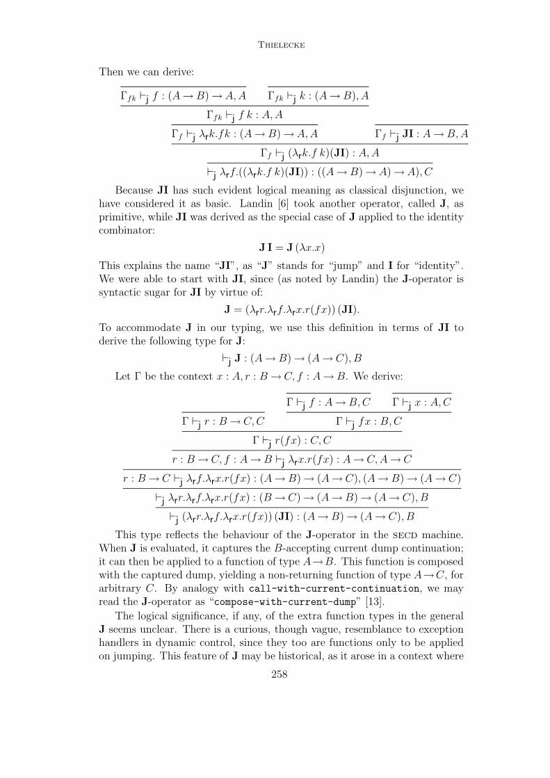
Thielecke

Then we can derive:

Γfk j f : (A → B) → A,A Γfk j k : (A → B), A

Γfk j f k : A,A

Γf j λrk.fk : (A → B) → A,A Γf j JI : A → B,A

Γf j (λrk.f k)(JI) : A,A

j λrf.((λrk.f k)(JI)) : ((A → B) → A) → A), C

Because JI has such evident logical meaning as classical disjunction, wehave considered it as basic. Landin [6] took another operator, called J, asprimitive, while JI was derived as the special case of J applied to the identitycombinator:

J I = J (λx.x)

This explains the name “JI”, as “J” stands for “jump” and I for “identity”.We were able to start with JI, since (as noted by Landin) the J-operator issyntactic sugar for JI by virtue of:

J = (λrr.λrf.λrx.r(fx)) (JI).

To accommodate J in our typing, we use this definition in terms of JI toderive the following type for J:

j J : (A → B) → (A → C), B

Let Γ be the context x : A, r : B → C, f : A → B. We derive:

Γ j r : B → C,C

Γ j f : A → B,C Γ j x : A,C

Γ j fx : B,C

Γ j r(fx) : C,C

r : B → C, f : A → B j λrx.r(fx) : A → C,A → C

r : B → C j λrf.λrx.r(fx) : (A → B) → (A → C), (A → B) → (A → C)

j λrr.λrf.λrx.r(fx) : (B → C) → (A → B) → (A → C), B

j (λrr.λrf.λrx.r(fx)) (JI) : (A → B) → (A → C), B

This type reflects the behaviour of the J-operator in the secd machine.When J is evaluated, it captures the B-accepting current dump continuation;it can then be applied to a function of type A→B. This function is composedwith the captured dump, yielding a non-returning function of type A→C, forarbitrary C. By analogy with call-with-current-continuation, we mayread the J-operator as “compose-with-current-dump” [13].

The logical significance, if any, of the extra function types in the generalJ seems unclear. There is a curious, though vague, resemblance to exceptionhandlers in dynamic control, since they too are functions only to be appliedon jumping. This feature of J may be historical, as it arose in a context where

258

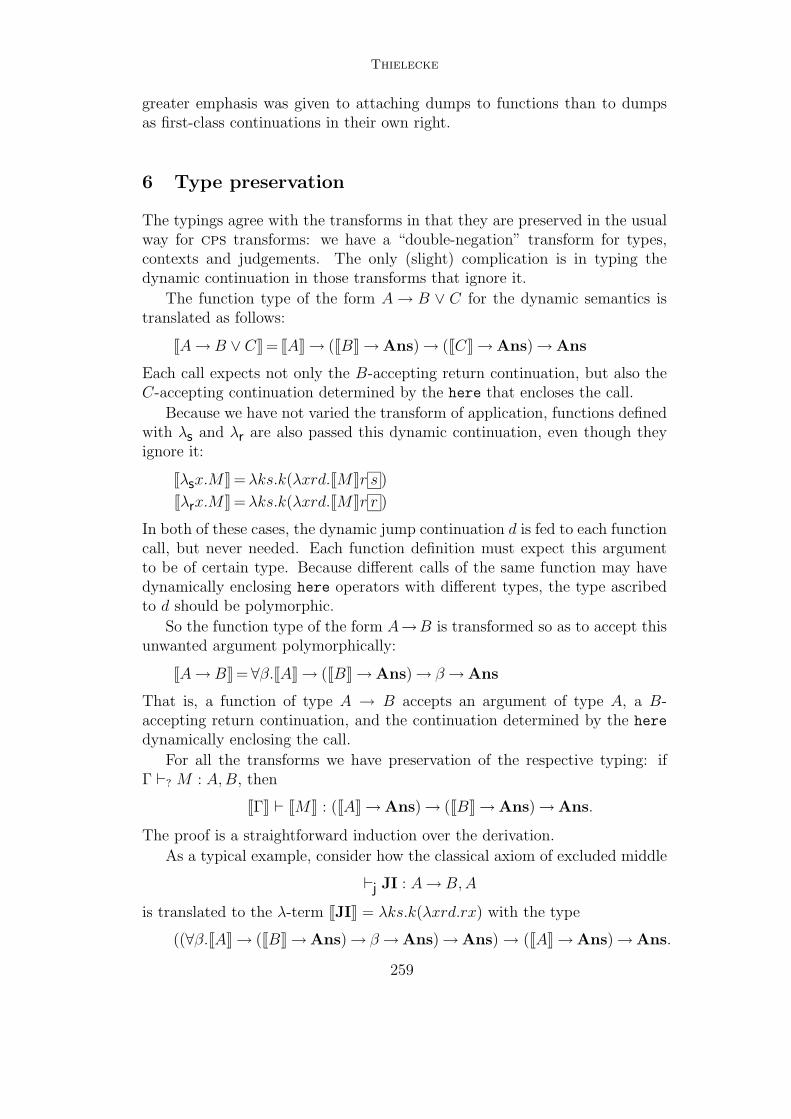
Thielecke

greater emphasis was given to attaching dumps to functions than to dumpsas first-class continuations in their own right.

6 Type preservation

The typings agree with the transforms in that they are preserved in the usualway for cps transforms: we have a “double-negation” transform for types,contexts and judgements. The only (slight) complication is in typing thedynamic continuation in those transforms that ignore it.

The function type of the form A → B ∨ C for the dynamic semantics istranslated as follows:

[[A → B ∨ C]] = [[A]] → ([[B]] → Ans) → ([[C]] → Ans) → Ans

Each call expects not only the B-accepting return continuation, but also theC-accepting continuation determined by the here that encloses the call.

Because we have not varied the transform of application, functions definedwith λs and λr are also passed this dynamic continuation, even though theyignore it:

[[λsx.M ]] = λks.k(λxrd.[[M ]]r s )

[[λrx.M ]] = λks.k(λxrd.[[M ]]r r )

In both of these cases, the dynamic jump continuation d is fed to each functioncall, but never needed. Each function definition must expect this argumentto be of certain type. Because different calls of the same function may havedynamically enclosing here operators with different types, the type ascribedto d should be polymorphic.

So the function type of the form A→B is transformed so as to accept thisunwanted argument polymorphically:

[[A → B]] = ∀β.[[A]] → ([[B]] → Ans) → β → Ans

That is, a function of type A → B accepts an argument of type A, a B-accepting return continuation, and the continuation determined by the here

dynamically enclosing the call.

For all the transforms we have preservation of the respective typing: ifΓ `? M : A,B, then

[[Γ]] ` [[M ]] : ([[A]] → Ans) → ([[B]] → Ans) → Ans.

The proof is a straightforward induction over the derivation.

As a typical example, consider how the classical axiom of excluded middle

j JI : A → B,A

is translated to the λ-term [[JI]] = λks.k(λxrd.rx) with the type

((∀β.[[A]] → ([[B]] → Ans) → β → Ans) → Ans) → ([[A]] → Ans) → Ans.

259

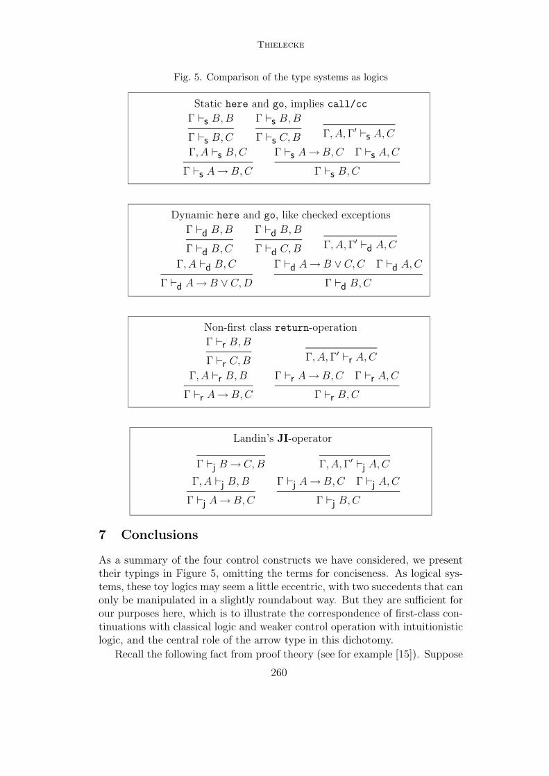
Thielecke

Fig. 5. Comparison of the type systems as logics

Static here and go, implies call/cc

Γ `s B,B

Γ `s B,C

Γ `s B,B

Γ `s C,B Γ, A, Γ′ `s A,C

Γ, A `s B,C

Γ `s A → B,C

Γ `s A → B,C Γ `s A,C

Γ `s B,C

Dynamic here and go, like checked exceptions

Γ `d B,B

Γ `d B,C

Γ `d B,B

Γ `d C,B Γ, A, Γ′ `d A,C

Γ, A `d B,C

Γ `d A → B ∨ C,D

Γ `d A → B ∨ C,C Γ `d A,C

Γ `d B,C

Non-first class return-operation

Γ `r B,B

Γ `r C,B Γ, A, Γ′ `r A,C

Γ, A `r B,B

Γ `r A → B,C

Γ `r A → B,C Γ `r A,C

Γ `r B,C

Landin’s JI-operator

Γ j B → C,B Γ, A, Γ′j A,C

Γ, A j B,B

Γ j A → B,C

Γ j A → B,C Γ j A,C

Γ j B,C

7 Conclusions

As a summary of the four control constructs we have considered, we presenttheir typings in Figure 5, omitting the terms for conciseness. As logical sys-tems, these toy logics may seem a little eccentric, with two succedents that canonly be manipulated in a slightly roundabout way. But they are sufficient forour purposes here, which is to illustrate the correspondence of first-class con-tinuations with classical logic and weaker control operation with intuitionisticlogic, and the central role of the arrow type in this dichotomy.

Recall the following fact from proof theory (see for example [15]). Suppose

260

Thielecke

one starts from a presentation of intuitionistic logic with sequents of the formΓ ` ∆. If a rule like the following is added that allows →-introduction even ifthere are multiple succedents, the logic becomes classical.

Γ, A ` B, ∆

Γ ` A → B, ∆

In continuation terms, the significance of this rule is that the function clo-sure of type A → B may contain any of the continuations that appear in ∆;to use the jargon, these continuations become “reified”. The fact that thelogic becomes classical means that once we can have continuations in func-tion closures, we gain first-class continuations and thereby the same power ascall/cc. We have this form of rule for static here and go; though not for JI,since JI as the excluded middle is already blatantly classical by itself.

But the logic remains intuitionistic if the →-introduction is restricted. Therule for this case typically admits only a single formula on the right:

Γ, A ` B

Γ ` A → B, ∆

Considered as a restriction on control operators, this rule prohibits λ-abstractionfor terms that contain free continuation variables. There are clearly other pos-sibilities how we can prevent assumptions from ∆ to become hidden (in thatthey can be used in the derivation of A→B without showing up in this typeitself). We could require these assumptions to remain explicit in the arrowtype, by making ∆ a singleton that either coincides with the B on the rightof the arrow, or is added to it:

Γ, A `r B,B

Γ `r A → B,C

Γ, A `d B,C

Γ `d A → B ∨ C,D

These are the rules for →-introduction in connection with the return-operation,and dynamic here and go, respectively. Neither of which gives rise to first-class continuations, corresponding to the fact that with these restrictions on→-introduction the logics remain intuitionistic.

The distinction between static and dynamic control in logical terms ap-pears to be new, as is the logical explanation of Landin’s JI-operator.

7.1 Related work

Following Griffin [3], there has been a great deal of work on classical typesfor control operators, mainly on call/cc or minor variants thereof. A similarcps transforms for dynamic control (exceptions) has appeared in [5], albeitfor a very different purpose. Felleisen describes the J-operator by way of cps,but since his transform is not double-barrelled, J means something differentin each λ [2]. Variants of the here and go operators are even older than thenotion of continuation itself: the operations valof and resultis from cpl

later appeared in Strachey and Wadsworth’s report on continuations [11,12].

261

Thielecke

These operators led to the modern return in C. As we have shown here, theylead to much else besides if combined with different flavours of λ.

7.2 Further work

In this paper, control constructs were compared by cps transforms and typingof the source. A different, but related approach compares them by typing inthe target of the cps [1]. On the source, we have the dichotomy betweenintuitionistic and classical typing, whereas on the target, the distinction isbetween linear and intuitionistic. We hope to relate these in further work.

References

[1] Berdine, J., P. W. O’Hearn, U. Reddy and H. Thielecke, Linearly usedcontinuations, in: A. Sabry, editor, Proceedings of the 3rd ACM SIGPLANWorkshop on Continuations, 2001.

[2] Felleisen, M., Reflections on Landin’s J operator: a partly historical note.,Computer Languages 12 (1987), pp. 197–207.

[3] Griffin, T. G., A formulae-as-types notion of control, in: Proc. 17th ACMSymposium on Principles of Programming Languages, San Francisco, CA USA,1990, pp. 47–58.

[4] Kelsey, R., W. Clinger and J. Rees, editors, Revised5 report on the algorithmiclanguage Scheme, Higher-Order and Symbolic Computation 11 (1998), pp. 7–105.

[5] Kim, J., K. Yi and O. Danvy, Assessing the overhead of ML exceptions byselective CPS transformation, in: Proceedings of the 1998 ACM SIGPLANWorkshop on ML, 1998.

[6] Landin, P. J., A generalization of jumps and labels, Report, UNIVAC SystemsProgramming Research (1965).

[7] Landin, P. J., A generalization of jumps and labels, Higher-Order and SymbolicComputation 11 (1998), reprint of [6].

[8] Plotkin, G., Call-by-name, call-by-value, and the λ-calculus, TheoreticalComputer Science 1 (1975), pp. 125–159.

[9] Reynolds, J. C., Definitional interpreters for higher-order programminglanguages, in: Proceedings of the 25th ACM National Conference (1972), pp.717–740.

[10] Riecke, J. G. and H. Thielecke, Typed exceptions and continuations cannotmacro-express each other, in: J. Wiedermann, P. van Emde Boas and M. Nielsen,editors, Proceedings 26th International Colloquium on Automata, Languagesand Programming (ICALP), LNCS 1644 (1999), pp. 635–644.

262

Thielecke

[11] Strachey, C. and C. P. Wadsworth, Continuations: A mathematical semanticsfor handling full jumps, Monograph PRG-11, Oxford University ComputingLaboratory, Programming Research Group, Oxford, UK (1974).

[12] Strachey, C. and C. P. Wadsworth, Continuations: A mathematical semanticsfor handling full jumps, Higher-Order and Symbolic Computation 13 (2000),pp. 135–152, reprint of [11].

[13] Thielecke, H., An introduction to Landin’s “A generalization of jumps andlabels”, Higher-Order and Symbolic Computation 11 (1998), pp. 117–124.

[14] Thielecke, H., On exceptions versus continuations in the presence of state,in: G. Smolka, editor, Programming Languages and Systems, 9th EuropeanSymposium on Programming, ESOP 2000,, number 1782 in LNCS (2000), pp.397–411.

[15] Troelstra, A. S. and H. Schwichtenberg, “Basic Proof Theory,” CambridgeUniversity Press, 1996.

263

264

MFPS 17 Preliminary Version

Distance and Measurement in Domain Theory

Pawe l Waszkiewicz

School of Computer Science

The University of Birmingham

Birmingham, United Kingdom

Abstract

We investigate the notion of distance on domains. In particular, we show that

measurement is a fundamental concept underlying partial metrics by proving that a

domain in its Scott topology is partially metrizable only if it admits a measurement.

Conversely, the natural notion of a distance associated with a measurement not only

yields meaningful partial metrics on domains of essential importance in computa-

tion, such as IR, �1 and P!, it also serves as a useful theoretical device by allowing

one to establish the existence of partial metrics on arbitrary !-continuous dcpo's.

1 Introduction

The theory by Keye Martin, introduced in [5], investigates domains equipped

not only with order but also with a quantitative notion of measurement. Thetheory is easy to understand, being based on the \informatic" intuition be-

hind domain theory. It is widely applicable. Most of the domains arising

in applications of domain theory have measurements, including the class ofall countably based domains. Two central notions of the theory are a mea-

surement and the �-topology called here the Martin topology. The last one isHausdor� on a domain and �ner than both Scott and Lawson topologies. It

is well-suited for computation: both continuity and completeness of a domain

can be described in terms of the Martin topology.

The main theme of this paper is the study of the notion of distance on

domains. Our work in this direction is very much inspired by questions posedby Reinhold Heckmann in [4] and Keye Martin in [5]. One obvious candidate

for a distance on domains is a partial metric such that the partial metrictopology agrees with the Scott topology of the induced order (see Section 2.2

for de�nitions). Another one is a symmetric map d� built from a measurement

� by a standard construction.

1Email: P.Waszkiewicz@cs.bham.ac.uk

This is a preliminary version. The �nal version will be published inElectronic Notes in Theoretical Computer Science

URL: www.elsevier.nl/locate/entcs

Waszkiewicz

The �rst problem of Heckmann's is to characterize partial metric spaces

which are continuous dcpo's with respect to the induced order and such that

the Scott topology and the partial metric topology agree. The other challenge

is to show which continuous dcpo's are partially metrizable.

We show that answers to both questions can be achieved by introducing

methods of measurement theory into the study of partial metric spaces. In

Section 3 we show that a continuous poset, which is partially metrizable in

its Scott topology must admit a measurement. Under some additional, mild

restrictions, the converse also holds: if the self-distance mapping for the partial

metric is a measurement, then as a consequence, the partial metric topology

agrees with the Scott topology.

Our thesis is that d�, called here the distance function associated with a

measurement �, deserves its name. We study its basic properties in Section

4. It is well-known [5] that d� induces the Scott topology. We prove thatit also encodes the underlying order, in the same fashion as partial metricsdo. Therefore, it is natural to ask if d� is a partial metric. We demonstrate

(see Section 5) that for arbitrary measurements the answer is positive fora restricted class of domains, which is, however, large enough to advance

O'Neill's construction from [7]. Our �nal argument in favour of d� being adistance between elements of a domain is presented in the last section. Weshow that every !-continuous dcpo is partially metrizable and the partial

metric is the distance function d� associated with some measurement � on thedomain. This result solves the second problem of Heckmann's for the class ofall countably based domains.

1.1 Convention

In the paper we adopt the following convention: original results are the num-

bered ones unless they are acknowledged explicitly. For instance, all the ex-

amples of measurements on domains from Section 2.5 are taken from [5].

2 Background

2.1 Domain theory

We review some basic notions from domain theory, mainly to �x the language

and notation. See [1] for more information. Let P be a poset. A pair of

elements x; y 2 P is consistent (bounded) if there exists an element z 2 P

such that z w x; y. We say that a poset is bounded-complete if each bounded

pair of elements has a supremum. A subset A � P of P is directed if it is

nonempty and any pair of elements of A has an upper bound in A. If a directed

set A has a supremum, it is denotedF

"A. A poset P in which every directed

set has a supremum is called a dcpo.

Let x and y be elements of a poset P . We say that x approximates (is

way-below) y if for all directed subsets A of P , y vF

"A implies x v a for

266

Waszkiewicz

some a 2 A. We denote it as x � y. Now, ##x is the set of all approximants

of x below it. ""x is de�ned dually. We say that a subset B of a dcpo P is a

(domain-theoretic) basis for P if for every element x of P , the set ##x \ B is

directed with supremum x. A poset is called continuous if it has a basis. It

can be shown that a poset P is continuous i� ##x is directed with supremum

x, for all x 2 P . A poset is called a domain if it is a continuous dcpo.

A subset U � P of a poset P is upper if x w y 2 U ) x 2 U . Upper sets

inaccessible by directed suprema form a topology called the Scott topology; it

is denoted �P . A domain admits a countable domain-theoretic basis i� the

Scott topology is second countable. In this case the domain is called an !-

continuous domain. The Scott topology encodes the underlying order: x v y

in P i� 8U 2 �: (x 2 U ) y 2 U). This is the general de�nition of the so-

called specialisation order for a topology. The collection f""x j x 2 Dg forms

a basis for the Scott topology on a continuous poset D. The Scott topologysatis�es only weak separation axioms: it is always T0 on a poset but T1 only ifthe order is trivial. The topology is sober on a domain (a topological space is

sober i� it is T0 and every nonempty closed subset which is not the union oftwo closed proper subsets is the closure of a point). Sobriety of a space implies

that the underlying specialisation order is a dcpo. For continuous posets, beinga dcpo and sobriety of the Scott topology are equivalent conditions.

The poset [0;1)op �gures prominently in Martin's work and also in thisnote. It is a domain without least element. We use v to refer to its orderwhich is dual to the natural one, �, and try to avoid the latter entirely. (� is

used in this paper whenever we work with [0;1).)

2.2 Partial metrics

We will brie y review basic de�nitions and facts about partial metric spaces

from Heckmann's [4] and Matthew's articles [6].

A partial metric on a set X is a map p : X � X ! [0;1) which satis�es

for all x; y; z 2 X,

1. p(x; y) = p(y; x) (symmetry),

2. p(x; y) = p(x; x) = p(y; y) implies x = y (T0 separation axiom),

3. p(x; y) � p(x; z) + p(z; y)� p(z; z) (�]),

4. p(x; x) � p(x; y) (SSD - \small self-distances").

If we abandon Axiom 4, p is called a weak partial metric. From the topological

point of view, weak partial metrics and partial metrics are equivalent since for

every weak partial metric p there is a corresponding one which satis�es SSD

[4], given by p0

(x; y) := maxfp(x; y); p(x; x); p(y; y)g.

The topology �p induced by the partial metric p is the topology which has

267

Waszkiewicz

a basis consisting of open balls of the form

B"(x) := fy 2 X j p(x; y) < p(x; x) + "g

for an x 2 X and a radius " > 0. The de�nition is well-formed since the

collection of open balls indeed forms a basis for a topology on X.

The name \T0 separation axiom" is justi�ed by the fact that it is a nec-

essary and suÆcient condition for X to be a T0 space w.r.t. �p. It is not

Hausdor� in general, as the example of the formal ball model shows. There-

fore, the specialisation order v�P of �p will be non-trivial in general.

All of the �p-open sets, the open balls among them, are upper sets with

respect to the order.

We have that the following are equivalent for all x; y 2 X:

1. x v�P y,

2. p(x; y) = p(x; x),

3. 8" > 0 y 2 B"(x).

We will say x vp y if one of the above conditions holds.

A weighted quasi-metric on a set X is a pair of maps (q; w) consisting ofa quasi-metric q:X2 ! [0;1) (satis�es all metric axioms but symmetry) anda weight function w:X ! [0;1) where for all x; y 2 X, q(x; y) + w(x) =

q(y; x) + w(y). q induces order and topology in the usual manner: for allx; y 2 X, x vq y i� q(x; y) = 0 and Bq

"(x) = fy 2 X j q(x; y) < "g is a basisfor the induced topology �q. Matthews [6] proves that there is an algebraic

equivalence between a partial metric p onX and a weighted quasi-metric (q; w)given by p(x; y) := q(x; y)+w(x) and conversely q(x; y) := p(x; y)�w(x) and,

moreover, p and q induce the same order and topology. We will exploit thisin the last theorem of the paper.

Finally, for every partial metric space (X; p), if X is equipped with thetopology �p induced by p and [0;1)op with the Scott topology, then the map-ping p : X � X ! [0;1)op is continuous. Since every continuous map is

monotone with respect to the specialisation orders of its domain and codomain,

p : X�X ! [0;1)op and the corresponding weight function w : X ! [0;1)op

are monotone. This is one of the reasons why one can hope for the weight(self-distance) function to be a measurement.

2.3 Martin's theory

We give a summary of the main elements of Keye Martin's theory of measure-ments on domains. Our main reference is [5].

Let P be a poset and E a domain. For a monotone mapping �:P ! E

and any x 2 P , " 2 E we de�ne

�"(x) := fy 2 P j y v x ^ "� �yg = ��1(""") \ #x:

268

Waszkiewicz

We say that �"(x) is the set of elements of P which are "-close to x 2 P .

Since in most cases we assume E = [0;1)op, we read "� �(y) as �(y) < " in

the natural order, which matches the intuition behind the name of �"(x). The

map � can be thought of as a quantitative measure of a relative \distance"

between elements in P . Immediately we have that �"(x) 6= ; i� x 2 �"(x) and

for any y 2 P , if y 2 �"(x), then y 2 �"(y) � �"(x).

We say that a monotone mapping �:P ! E induces the Scott topology on a

subset X of a poset P if 8U 2 �P 8x 2 X: x 2 U ) (9" 2 E) x 2 �"(x) � U .

We denote it as � �!X �P . If X = P , we write � �! �P , which reads: �

induces the Scott topology everywhere (on P ).

In the paper, the following observation will often be referred to as the

measurement property: for a map �:P ! [0;1)op on a continuous poset P

and for any X � P , the following are equivalent:

(i) � is Scott-continuous and induces the Scott topology everywhere on X,(ii) for all x 2 X and all subsets S � ##x, S is directed with supremum x i�Ff�s j s 2 Sg = �x.

It is not hard to show that the identity mapping on a domain P inducesthe Scott topology everywhere on P . Moreover, the property is preserved by

the composition of maps. A measurement on a continuous poset D is a Scott-continuous mapping �:D! [0;1)op which induces the Scott topology on its

kernel ker� := fx 2 D j �(x) = 0g.

Martin's theory has a rich topological dimension. The Martin topology

(also called the � topology) arises naturally in the consideration of measure-ments. For any monotone mapping �:D! E between domains, the collectionf�"(x) j x 2 D; " 2 Eg forms a basis for a topology on D. In particular, if

� is taken to be the identity map on D, we obtain a topology with a basisf""x\#y j x; y 2 Dg. We call this topology the Martin topology on D. The fol-

lowing important Invariance Theorem holds: if �:D! E is Scott-continuous,then � induces the Scott topology on D i� f�"(x) j x 2 D; " 2 Eg is a basisfor the Martin topology on D. That is, no matter how we measure a domain,

all measurements give rise to the same � topology on the domain. The Martin

topology is always Hausdor� on a domain. The study of its properties is thesubject of a chapter in Martin's thesis [5].

In our paper we work on posets equipped with a particularly pleasant

class of measurements which induce the Scott topology everywhere on theirdomains. We are able to characterize both the order (see Sections 4) and

completeness of a domain strictly in terms of the measurement.

2.4 Completeness

For any topology � , the collection of intersections C \O of a closed set C and

an open set O of � forms a basis of a topology, the so-called b-topology for� . S�underhauf [8] shows that � is sober i� every observative net converges in

the b-topology for � . (A net (xi)i2I is observative if for all i 2 I and for all

269

Waszkiewicz

U 2 � , xi 2 U implies that the net is eventually in U .) In the case of posets

with measurements, we can con�ne our attention to observative sequences:

Lemma 2.1 Let P be a continuous poset with a measurement �:P ! [0;1)op

such that ��!�P . The Scott topology on P is �rst-countable.

Proof. P is �rst countable since f"��x+ 1

n

(x) j n 2 Ng is a countable neigh-

bourhood base at x 2 P . 2

It comes as no surprise that:

Proposition 2.2 The Martin topology is the b-topology for the Scott topology

on a continuous poset P .

Proof. The collection f""x \ #y j x; y 2 Pg is a basis for the Martin topology

on P . Thus, the Martin topology is always coarser than the b-topology. Toprove the converse, denote the b-topology for the Scott topology by � and let

x 2 U 2 � . We can assume U is a basic-open set in � and hence U = O \ C,where O is a Scott-open set and C is Scott-closed. Let us choose an elementy 2 U way-below x such that y 2 O. Also, y 2 C, since C is downward closed.

Consequently, y 2 U . We claim that the set A := ""y \ #x is a subset of U .Indeed, if z 2 A, then z 2 ""y � O. Also, z 2 #x � C. Therefore, z 2 U .

Since A is basic-Martin open, we are done. 2

Therefore, Martin's Invariance Theorem states that the b-topology for theScott topology on P can be constructed from a measurement with ��! �P(the proof of the Theorem holds verbatim, even if P is not a dcpo). Now,

S�underhauf's result gives that a continuous poset is sober (equivalently: is adcpo) i� every observative sequence in P Martin-converges in P . However, it

happens that with much simpler reasoning we can prove a stronger result. We

need to know a few simple facts about convergence in the Martin topology, all

proved in [5]. Firstly, given a measurement �:P ! [0;1)op on a continuous

poset P , a sequence (xn) converges to an x 2 P in the Martin topology onP i� lim�xn = �x and (xn) is eventually in #x. Secondly, a sequence (xn)

Martin-converges to an x i� it Scott-converges and (xn) is eventually in #x.

Lemma 2.3 A continuous poset P with a measurement �:P ! [0;1)op with

��!�P is a dcpo i� every increasing sequence (xn) Martin-converges in P .

Proof. Let (xn) be a sequence with x =F

"xn. Since � is Scott-continuous,

�x = �(G

"xn) =Gf�xn j n 2 Ng = lim

n!1�xn:

Since xn v x for every n 2 N , (xn) Martin-converges. The proof of the

converse is essentially the content of Corollary 3.1.3 of [5] and we give it onlyfor the sake of completeness: Martin-convergence of (xn) to x implies that the

sequence is eventually below x. Since the sequence is increasing, all xn are

270

Waszkiewicz

below x. Let u be another upper bound for the sequence. For every Scott-

open set U around x, there exists k such that xk 2 U , by Scott-convergence.

Now, since U is upper, xk v u 2 U . This proves x v u. 2

We conclude this section with a summary of results:

Theorem 2.4 Let P be a continuous poset with a measurement �:P ! [0;1)op

with ��!�P . The following are equivalent:

(i) the Scott topology on P is sober,

(ii) P is a dcpo,

(iii) all increasing sequences converge in the Scott topology on P ,

(iv) all increasing sequences converge in the Martin topology on P ,

(v) all observative sequences converge in the Martin topology on P . 2

2.5 Examples of domains with measurements

Cantor set model �1. Let �1 denote the set of all �nite and in�nite wordsover a �nite alphabet �, with the pre�x ordering. This is an !-algebraic

domain. For all x; y 2 �1, x� y holds i� x v y and x is �nite. The mapping

1

2j�j: �1 ! [0;1)op

where j � j : �1 ! N [ f1g takes a string to its length is a measurement on�1. Moreover, it induces the Scott topology everywhere on �1.

The interval domain IR. The collection IR of compact intervals of thereal line ordered under reverse inclusion is an !-continuous domain. The

supremum of a directed set S � IR isTS and for all intervals x; y 2 IR

we have x � y i� x is contained in the interior of y. The length function

j � j : IR ! [0;1)op given by jxj = x� x, where x = [x; x] 2 IR, is a measure-

ment on IR. It induces the Scott topology everywhere on IR.

The powerset of naturals P!. The collection of all subsets of N ordered by

inclusion is an !-algebraic domain. The supremum of a directed set S � P!

isSS and for all elements x; y of P! the approximation relation is given by

x� y i� x � y and x �nite. The mapping j � j : P! ! [0;1)op given by

jxj = 1�X

n2x

1

2n+1

is a measurement on P!. It induces the Scott topology everywhere on P!.

The formal ball model BX, introduced in [2]. The mapping � : BX !

[0;1)op given by �(x; r) = r is a measurement on BX. It induces the Scott

topology everywhere on BX.

271

Waszkiewicz

The domain of �nite lists [S] over a set S. A list x over a set S is a map

x: f1; 2; :::; ng ! S for n � 0. Informally, for x; y 2 [S], y is a sublist of x if

y matches some convex subset of x, e.g. [a; b] is a sublist of [c; a; b; d], while

[a; d] is not. We de�ne a partial order on [S] by x v y i� y is a sublist of x.

With this order, [S] is an algebraic dcpo, where every element is compact. [S]

is !-continuous i� S is countable. The length of the list, len: [S] ! N , given

by len(x) := jdom(x)j (cardinality of the domain of x) is a measurement on

[S], which induces the Scott topology everywhere on [S].

In all the examples above, the kernel of the measurement is precisely the set

of maximal elements. However, we do not know if for arbitrary !-continuous

dcpo, the set of maximals is the kernel of some measurement on the domain.

This is already a 3-year old problem. Below, we show that it is the condition

on the kernel which causes the diÆculty, since it is easy to �nd a measurement

on a domain with countable basis (with possibly empty kernel).

Example 2.5 [5] For any continuous dcpo D with a countable basis fUn j

n 2 Ng for the Scott topology, a mapping �:D! [0;1)op given by

�(x) := 1�X

fn2N:x2Ung

1

2n+1

is a measurement which induces the Scott topology everywhere on D.

3 The necessity of measurement on partially metrizable

domains

In this paper, we are mainly concerned with the case when a partial metric

topology is the Scott topology of the induced order, �p = � in symbols. Wedemonstrate that such a class of partial metrics is intimately connected to

measurements. We give a construction of a measurement from a given partial

metric with �p = �X on an arbitrary set X. Precisely, for a partial metric p ona set X, the self-distance mapping �:X ! [0;1)op given by �(x) := p(x; x)

for all x 2 X is Scott-continuous and induces the Scott-topology everywhereon X.

Moreover, it happens that under some mild, computationally meaningful

restrictions on an underlying poset X, the converse also holds: if the self-

distance map � is a measurement which induces the Scott topology every-where, then �p = �.

We use �X � �p to denote the fact that the partial metric topology is largerthan the Scott topology of the induced order vp. The meaning of �p � �X isanalogous. Also, in this section, ��! � means that the mapping � induces

the Scott topology everywhere on X.

Theorem 3.1 Let (X; p) be a partial metric space such that the Scott topology

of the order vp agrees with the partial metric topology �p. Then the self-

272

Waszkiewicz

distance map �:X ! [0;1)op is Scott-continuous and has property ��!�.

Proof. First, we will show that if �X � �p, then � �! �. Indeed, let x 2

U 2 �X . Since �X � �p, there exists an " > 0 such that x 2 B"(x) � U .

De�ne Æ := �(x) + ". Since �(x) < Æ, x 2 �Æ(x). Now, let y 2 �Æ(x). Since

p(x; y) � �(y) as yvpx and �(y) < Æ = �(x) + ", we have p(x; y) < �(x) + ".

This means y 2 B"(x). Therefore �Æ(x) � B"(x).

Now, it remains to show that if �p � �X , then the self-distance map �:X !

[0;1)op is Scott-continuous. For, since p : X�X ! [0;1)op is �p-continuous,

also � is �p-continuous. The Scott-continuity of � follows immediately from

the assumption. 2

Therefore, we obtained a necessary condition for partial metrizability of

the Scott topology on continuous posets.

Corollary 3.2 Every partially metrizable continuous poset admits a measure-

ment which induces the Scott topology everywhere.

It happens that there is a class of partial metric spaces where inducing theScott topology by the self-distance map is equivalent to the agreement of theScott and partial metric topologies.

De�nition 3.3 We call a partial metric space stable if

8x; y 2 X: p(x; y) =Gf�z j z vp x; yg:

Notice that the last condition is equivalent to

8x; y 2 X 8" > 0 9z vp x; y: �(z) < p(x; y) + ":

Moreover, if X is a continuous poset with respect to the induced order, then

stability can be written as 8x; y 2 X: p(x; y) =Ff�z j z �p x; yg, where �p

is the way-below relation obtained from the order vp.

Theorem 3.4 Let (X; p) be a partial metric space such that:

1. X is stable, and

2. the induced order vp makes X a continuous poset.

Then the Scott topology of the order vp agrees with the partial metric topology

�p i� the self-distance map �:X ! [0;1)op is a measurement with property

��!�.

Proof. The proof consists of two observations. The �rst one states that, if

(X; p) is a stable space, then �X � �p holds i� ��!�. ()) has already been

shown in the proof of the preceding theorem. For the converse, let x 2 U 2 �X .By ��!�, we can assume x 2 �Æ(x) � U , where Æ := �(x)+" for some " > 0.

Set "0 := 12". We want to show B"0(x) � "(�Æ(x)). Let y 2 B"0(x). Then by

273

Waszkiewicz

de�nition, p(x; y) < �(x) + "0. By assumption, there exist z vp x; y such that

we have

�(z) < p(x; y) + "0 < �(x) + 2"0 = �(x) + " = Æ:

Hence we have shown that z 2 �Æ(x). Moreover, since z vp y, y 2 "�Æ(x).

Therefore the claim that B"0(x) � "(�Æ(x)) is now proved. Consequently, we

have

x 2 B"0(x) � "�Æ(x) � "U = U;

which gives �X � �p. The proof of the �rst observation is completed.

The second one states that if (X; p) is a partial metric space such that

the induced order vp makes X a continuous poset, then �p � �X i� the self-

distance map �:X ! [0;1)op is Scott-continuous. For ((), let x 2 V 2 �p.

Take any open ball around x in V , that is, choose " > 0 such that x 2 B"(x) �

V . It is easy to show that x 2 �Æ(x) � B"(x) � V , where Æ := �(x)+ ". Since

B"(x) is an upper set, x 2 "�Æ(x) � B"(x) � V . Finally, by continuity of X

and �, the set "�Æ(x) is Scott-open (see also the next section for more detailedexplanation). Therefore �p � �X .

The converse has already been shown in the proof of the preceding theo-rem. 2

4 The distance map associated with a measurement

In the last section we saw that whenever a partial metric induces the Scott

topology on the underlying domain, the domain admits a measurement whichinduces the Scott topology everywhere. This result tells us we should look tomeasurement in de�ning a notion of distance on domains. We start with a

standard construction from [5].

Given a continuous poset P equipped with a measurement �:P ! E with

��!�P one can de�ne a mapping d�:P2 ! E given by d�(x; y) :=

Ff�(z) j

z � x; yg, providing that any two elements x; y of P are bounded from below

and E is a dcpo. Martin proves that d� is Scott-continuous on P 2. Our thesisis that d� may serve as a distance function between elements of a domain. In

this section we examine basic properties of d�.

De�nition 4.1 Let P be a continuous poset with a measurement �:P !

[0;1)op. The map d� : P2 ! [0;1)op de�ned by

d�(x; y) :=Gf�(z) j z � x; yg

is the distance function associated with �.

Notice that for a continuous poset P with a measurement, we can alwaysassume that d� is de�ned: we simply scale the measurement to [0; 1)op by

��x := �x

1+�x, add bottom to P with ��? := 1 and study d�� .

d� induces a topology on P . The collection of open balls fB"(x) j x 2

P; " > 0g is a basis for the topology, where B"(x) := fy 2 P j d�(x; y) < "g.

274

Waszkiewicz

If �:P ! E is a Scott-continuous mapping on a continuous poset P with

��!�P , then f"�"(x) j x 2 P; " 2 Eg is a basis for the Scott topology on P .

Now, Martin proved that for all x 2 P and " > 0, B"(x) = "�"(x), that is, the

topology induced by d� is always the Scott topology. Thanks to this crucial

fact, from now on it is clear that d� is a computationally important object to

study.

First of all, we are going to show that whenever a continuous poset is

equipped with a measurement, the induced distance d� captures order between

elements. Let us start with a well-known fact:

Lemma 4.2 ([5]) Let P be a continuous poset with a monotone map �:P !

[0;1)op. The following are equivalent:

(i) � is Scott-continuous,

(ii) �x = d�(x; x) for any x 2 P ,

(iii) x v y ) d�(x; y) = �x for any x; y 2 P .

Theorem 4.3 Let P be a continuous poset with a measurement �:P ! [0;1)op

with ��!�P . Then for all x; y 2 P ,

x v y () d�(x; y) = �x:

Proof. ()) by Lemma 4.2. For (() assume d�(x; y) = �x. Let (xn) be asequence with xn � x; y and lim�xn = d�(x; y). Then lim�xn = �x and

by the measurement property, (xn) is directed with supremum x. Therefore,x =F

"xn v y. 2

Observe an immediate corollary of the result and Example 2.5. We are

able to characterize the order relation on arbitrary !-continuous dcpo.

Corollary 4.4 For any continuous dcpo D with a countable basis fUn j n 2

Ng for the Scott topology, x v y () d�(x; y) = �x, where �:D ! [0;1)op

is given in Example 2.5. 2

Now we have an elementary proof of some properties of d�. The �rst one,below, can be treated as the T0 axiom in the case when d� is a partial metric

on D. The second property states the antisymmetry of the order.

Corollary 4.5 With assumptions of Theorem 4.3, d� has the following prop-

erties:

1. d�(x; y) = �x = �y () x = y,

2. d�(x; y) = 0 () x = y 2 ker�. 2

The characterization of the order given in Theorem 4.3 reminds us of the

de�nition of the order induced by a partial metric. Therefore one can ask

when d� is a partial metric.

275

Waszkiewicz

5 When distance is a partial metric

We now try to justify the intuition that d� provides a measure of distance be-

tween elements of a domain. In particular, we start with a suÆcient condition

for d� to be a partial metric.

Proposition 5.1 Let P be a continuous poset with a measurement �:P !

[0;1)op with ��! �P . If for all consistent pairs a; b 2 P and for all upper

bounds r of a and b, there exists an s v a; b such that

�r + �s � �a+ �b;

then d�:P ! [0;1) is a partial metric on P such that its induced order agrees

with the order on P and the partial metric topology �p is the Scott topology on

P .

Proof. Proofs of this and next proposition are extensions of Martin's argu-ment in Corollary 5.4.1 of [5].

It is enough to prove that d� satis�es �]. Take any x; y; z 2 P . By de�nitionof d�, there exists an a v x; z and b v y; z such that

d�(x; z) +"

2� �a ^ d�(y; z) +

"

2� �b;

for any " > 0. Since a; b are consistent, there is s v a; b such that

d�(x; y) � d�(a; b) � �s � �a+ �b� �z:

Hence,d�(x; y) + �z � d�(x; y) + d�(y; z) + ";

for all " > 0. This proves that d� satis�es �]. Agreement of orders andtopologies claimed in the hypothesis follows from general properties of d�. 2

Notice that if P is bounded-complete and � is modular, that is, for allconsistent pairs x; y 2 P we have �(x t y) + �(x u y) = �x + �y, then the

conditions of the proposition hold and d� = �(x u y) is a partial metric onP . Hence we advanced the result by O'Neill [7] who gave a construction

of a partial metric from a valuation on a so called valuation space, i.e. on

a bounded-complete inf-semilattice. However, as our last result shows, theexistence of suprema and in�ma is not necessary.

Proposition 5.1 guarantees the existence of a partial metric which induces

the Scott topology on IR;�1 ;P! since their natural measurements are mod-

ular.

The mapping pIR: IR � IR ! [0;1) given by

pIR([x; x]; [y; y]) := maxfx; yg �minfx; yg

where [x; x]; [y; y] 2 IR, is a partial metric on IR.

276

Waszkiewicz

The mapping p�1 : �1 � �1 ! [0;1) given by

p�1(x; y) := 2�jrj;

where r is the largest common pre�x of x and y, is a partial metric on �1.

The mapping pP!:P! � P! ! [0;1) given by

pP!(x; y) := 1�X

n2x\y

2�(n+1)

is a partial metric on P!.

In more general cases, d� is usually no longer a partial metric. Sometimes,

however, d� still satis�es the classical triangle inequality for metrics.

Proposition 5.2 Let P be a continuous poset with a measurement �:P !

[0;1)op with ��!�P such that

9z v x; y: �z � �x+ �y:

Then d�:P ! [0;1) satis�es the triangle inequality and induces the Scott

topology on P .

Proof. The reasoning is essentially the same as in the proof of the preceding

Proposition. 2

Interestingly, in the case above, the restriction of d� to ker� is a metricwhich yields the relative Scott topology on ker�. This fact is investigatedin detail in Martin's thesis. Further generalization is still possible, but this

involves applying a valuable construction due to Frink [3] to the map d�, and

is beyond our present concern.

6 The existence of partial metrics on countably based

domains

The results in the last section make us think that d� may serve as a distance

map on domains only in restricted cases and hence is not a useful theoreticaldevice in establishing the existence of partial metrics. However, the following

result shows that this is not true. It also provides a practical illustration ofthe techniques developed in sections 3 and 4.

Theorem 6.1 Let D be an !-continuous dcpo. Then there is a Scott-continuous

partial metric p : D2 ! [0;1) such that

(i) vp=vD,

(ii) the Scott topology on D is the partial metric topology �p.

In short, all countably based domains are partially metrizable.

277

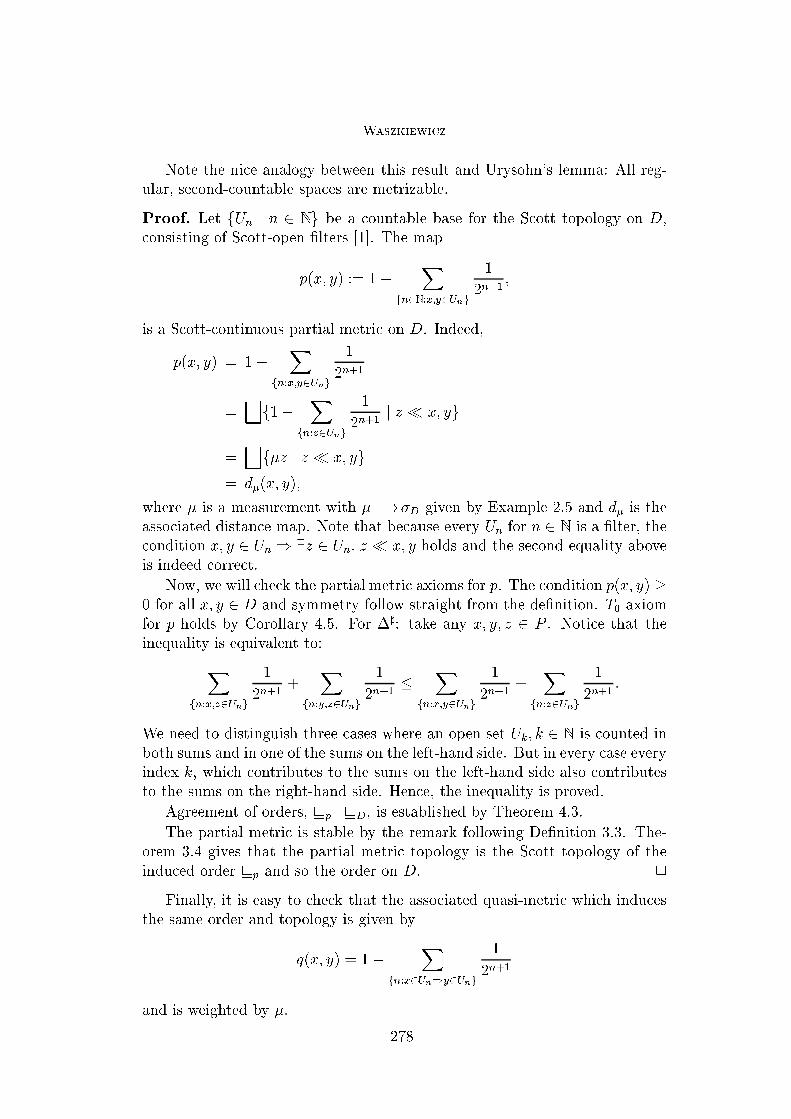
Waszkiewicz

Note the nice analogy between this result and Urysohn's lemma: All reg-

ular, second-countable spaces are metrizable.

Proof. Let fUn j n 2 Ng be a countable base for the Scott topology on D,

consisting of Scott-open �lters [1]. The map

p(x; y) := 1�X

fn2N:x;y2Ung

1

2n+1;

is a Scott-continuous partial metric on D. Indeed,

p(x; y) = 1�X

fn:x;y2Ung

1

2n+1

=Gf1�

X

fn:z2Ung

1

2n+1j z � x; yg

=Gf�z j z � x; yg

= d�(x; y);

where � is a measurement with ��!�D given by Example 2.5 and d� is theassociated distance map. Note that because every Un for n 2 N is a �lter, thecondition x; y 2 Un ) 9z 2 Un: z � x; y holds and the second equality above

is indeed correct.

Now, we will check the partial metric axioms for p. The condition p(x; y) �

0 for all x; y 2 D and symmetry follow straight from the de�nition. T0 axiomfor p holds by Corollary 4.5. For �]: take any x; y; z 2 P . Notice that the

inequality is equivalent to:

X

fn:x;z2Ung

1

2n+1+

X

fn:y;z2Ung

1

2n+1�

X

fn:x;y2Ung

1

2n+1+X

fn:z2Ung

1

2n+1:

We need to distinguish three cases where an open set Uk; k 2 N is counted in

both sums and in one of the sums on the left-hand side. But in every case everyindex k, which contributes to the sums on the left-hand side also contributes

to the sums on the right-hand side. Hence, the inequality is proved.

Agreement of orders, vp=vD, is established by Theorem 4.3.

The partial metric is stable by the remark following De�nition 3.3. The-orem 3.4 gives that the partial metric topology is the Scott topology of the

induced order vp and so the order on D. 2

Finally, it is easy to check that the associated quasi-metric which induces

the same order and topology is given by

q(x; y) = 1�X

fn:x2Un)y2Ung

1

2n+1

and is weighted by �.

278

Waszkiewicz

Acknowledgement

The author wishes to thank Achim Jung and Keye Martin for their valuable

criticisms and Dagmara Bogucka for her support and friendship.

References

[1] S. Abramsky and A. Jung. Domain theory. In S. Abramsky, D. M. Gabbay, and

T. S. E. Maibaum, editors, Handbook of Logic in Computer Science, volume 3,

pages 1{168. Clarendon Press, 1994.

[2] A. Edalat and R. Heckmann. A computational model for metric spaces.

Theoretical Computer Science, 193:53{73, 1998.

[3] A.H. Frink. Distance functions and the metrization problem. Bulletin of the

American Mathematical Society, 43:133{142, 1937.

[4] Reinhold Heckmann. Approximation of metric spaces by partial metric spaces.

Applied Categorical Structures, 7:71{83, 1999.

[5] Keye Martin. A Foundation for Computation. PhD thesis, Department of

Mathematics, Tulane University, New Orleans, LA 70118, 2000.

[6] Steve G. Matthews. Partial metric topology. In Proceedings of the 8th Summer

Conference on Topology and Its Application, volume 728, pages 176{185, 1992.

[7] Simon J. O'Neill. Partial metrics, valuations and domain theory. Research

Report CS-RR-293, Department of Computer Science, University of Warwick,

Coventry, UK, October 1995.

[8] Philipp S�underhauf. Sobriety in terms of nets. Applied Categorical Structures,

8:649{653, 2000.

279

Recent BRICS Notes Series Publications

NS-01-2 Stephen Brookes and Michael Mislove, editors.PreliminaryProceedings of the 17th Annual Conference on MathematicalFoundations of Programming Semantics, MFPS ’01,(Aarhus,Denmark, May 24–27, 2001), May 2001. viii+279 pp.

NS-01-1 Nils Klarlund and Anders Møller. MONA Version 1.4 — UserManual. January 2001. 83 pp.

NS-00-8 Anders Møller and Michael I. Schwartzbach.The XML Revo-lution. December 2000. 149 pp.

NS-00-7 Nils Klarlund, Anders Møller, and Michael I. Schwartzbach.Document Structure Description 1.0. December 2000. 40 pp.

NS-00-6 Peter D. Mosses and Hermano Perrelli de Moura, editors.Pro-ceedings of the Third International Workshop on Action Seman-tics, AS 2000,(Recife, Brazil, May 15–16, 2000), August 2000.viii+148 pp.

NS-00-5 Claus Brabrand. <bigwig> Version 1.3 — Tutorial. Septem-ber 2000. ii+92 pp.

NS-00-4 Claus Brabrand.<bigwig> Version 1.3 — Reference Manual.September 2000. ii+56 pp.

NS-00-3 Patrick Cousot, Eric Goubault, Jeremy Gunawardena, Mau-rice Herlihy, Martin Raussen, and Vladimiro Sassone, edi-tors. Preliminary Proceedings of the Workshop on Geometryand Topology in Concurrency Theory, GETCO ’00,(State Col-lege, USA, August 21, 2000), August 2000. vi+116 pp.

NS-00-2 Luca Aceto and Bjorn Victor, editors. Preliminary Proceedingsof the 7th International Workshop on Expressiveness in Concur-rency, EXPRESS ’00,(State College, Pennsylvania, USA, Au-gust 21, 2000), August 2000. vi+130 pp.

NS-00-1 Bernd Gartner. Randomization and Abstraction — Useful Toolsfor Optimization. February 2000. 106 pp.

NS-99-3 Peter D. Mosses and David A. Watt, editors.Proceedings of theSecond International Workshop on Action Semantics, AS ’99,(Amsterdam, The Netherlands, March 21, 1999), May 1999.iv+172 pp.