214 8 • GLOBAL DIVERSIFICATION AND EXTINCTION

Box 8. 1

CONSTRUCTION OF DIVERSITY CURVES

This box illustrates the construction of global diver­sity curves using methods discussed in the main text. The data for these curves, presented in Table 8.1, con­sist of 40 hypothetical genera whose first and last ap­pearances fall within the epochs of the Cenozoic; 21 of the taxa are extant (i.e., their "last appearance" is in the Recent). These data are used to construct a set of values, presented in Table 8.2, that provide the basis for the curves depicted in Figure 8.3.

An important assumption in the construction of all diversity curves, known aptly as the range-through assumption, is that a taxon remains extant for the en­tire interval between its first and last known occur­rences in the fossil record. Importantly, if a taxon that is represented in the fossil record is also extant today,

it is therefore assumed that the taxon ranged through the entire interval from its first appearance in the fos­sil record through the present day, even if its first ap­pearance is its only known fossil occurrence (i.e., it is a fossil singleton).

To calculate diversity by the methods illustrated here, we must first determine the number of origina­tions (N. orig1) and the number of extinctions (N. ext1)

in each interval. For example, in perusing Table 8.1, we can see that there were nine first appearances and one last appearance in the Paleocene. Therefore, in Table 8.2, N. orig1 for the Paleocene is 9, and N. ext1 is 1. Once these values have been determined for all inter­vals, diversity can be calculated for the standard and boundary-crosser methods (Figures 8.3a and 8.3b)

TABLE 8.1

Global Stratigraphic Ranges for a Set of Hypothetical Genera

First Last First Last Genus Appearance Appearance Genus Appearance Appearance

a Paleocene Recent u Pliocene Recent b Miocene Miocene v Oligocene Pleistocene c Paleocene Eocene w Eocene Eocene d Eocene Eocene X Pleistocene Recent e Oligocene Recent y Paleocene Paleocene f Pleistocene Recent z Miocene Pliocene g Oligocene Miocene a a Paleocene Miocene h Paleocene Eocene bb Eocene Recent 1 Pliocene Recent cc Pliocene Recent

J Eocene Eocene dd Pleistocene Pleistocene k Oligocene Pleistocene ee Pleistocene Recent 1 Pleistocene Recent ff Paleocene Eocene m Pleistocene Pleistocene gg Miocene Recent n Pliocene Recent hh Oligocene Recent 0 Miocene Recent 11 Paleocene Eocene p Paleocene Oligocene lJ Pleistocene Recent q Eocene Recent kk Pliocene Recent r Miocene Recent 11 Miocene Recent s Paleocene Eocene mm Pleistocene Recent t Pleistocene Recent nn Pleistocene Pleistocene

..

e ~

~ .... = ::E 1-4

Paleocene 60 Eocene 45

8.3 • CONSTRUCTION OF GLOBAL DIVERSITY CURVES

TABLE 8.2

Values and Equations Used to Calculate Diversity Curves for the Hypothetical Data from Table 8.1

-"'C "'C "'C 0

~ o£ "' ~ 0 "' ~

= 0 ::E btl ~ "'C 1-4 ~ "' fll 1-4

"' ~ ~ fll 0 fll CJ ~

~ fll

= CJ e ~ = 1-4 u "' ~ fll fll "' "' ~ I

= fll :s "' >-:s CJ "'C 0 = CJ

= "' ~ .... 0 CJ CJ co "'C ~ .... 0 CJ ~ "'C

"' :s bh ~ fll 0 "' = - = bh =

.... :s :s. CJ ..... = 0 = .... CJ 0 = rJ'} ..... .... ~ = CJ ~ 1-4 rJ'} ~ CJ ~ 0 co ....

bh ~ CJ

"' .... :s .... ~ ~ .... t.S co 0 :s = ~ = 0 .s= 0 ..... o£ ~ --.... .s= rJ'} ..::: CJ fll

~ ·~ .... .... ·~ .... ~ ~

·~ :s ·~ ~ ..... "' b] b] 0 b] ~ ..... o£ .... ~ o£ ..... .s= "'C ·t: ~ 't: ~ •t: ~ .... = ..... ..... . ....

0 ~ ~ 0 ~ ~ 0 ~ ~ :s i 2.-;. 0 i -,:- i i ~ i i ~ ~

9 1 1 9 8 0 8 9 2 9 Paleocene/Eocene 5 8 3 13 2 5 10 5 10 12 Eocene/ Oligocene

215

Oligocene 28 5 1 0 10 5 1 10 5 3 7 Oligocene/Miocene Miocene 14 6 3 1 15 5 2 14 6 7 10 Miocene/Pliocene Pliocene 4 5 1 0 17 5 1 17 5 6 8 Pliocene/Pleistocene Pleistocene 1 10 5 3 26 7 2 23 10 12 12 Pleistocene/Recent

Key: d1 = diversity in interval t d1- 1 = diversity in interval t - 1 d1; 1+1 = diversity at boundary between intervals t and t + 1 N. orig1 = number of originations in interval t N. ext1 = number of extinctions in interval t N. ext1_ 1 = number of extinctions in interval t - 1 N st = number of singletons in interval t

Standard Method for Calculating Diversity: d1 = d1_ 1 + N. orig1 - N. ext1-1

Boundary-Crosser Method for Calculating Diversity:

Example: When all data are included,

doligocene = dEocene + N. origoligocene - N. extEocene;· thus, doligocene = 13 + 5 - 8 = 10

d1; 1+1 = d1 - N. ext1

Example:

doligocene/Miocene = doligocene - N · extoligocene ; thus, doligocene/Miocene = 10 - 1 = 9

..

216 8 • GLOBAL DIVERSIFICATION AND EXTINCTION

Box 8.)' (continued)

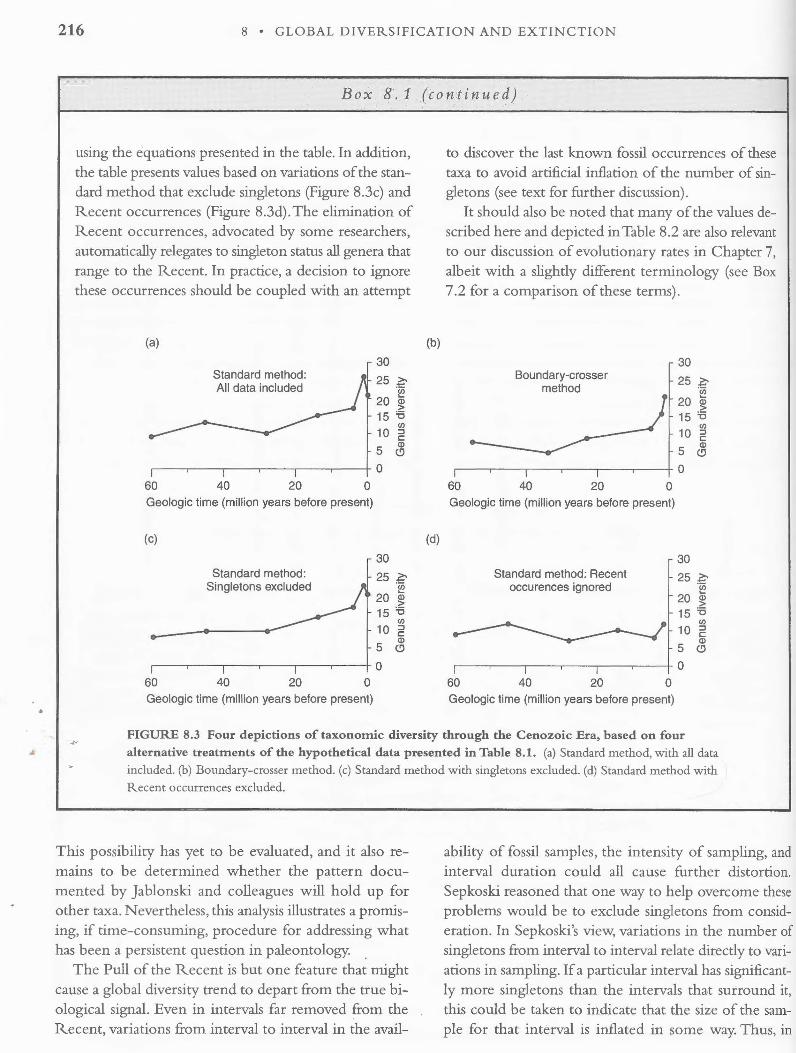
using the equations presented in the table. In addition, the table presents values based on variations of the stan­dard method that exclude singletons (Figure 8.3c) and Recent occurrences (Figure 8.3d). The elimination of Recent occurrences, advocated by some researchers, automatically relegates to singleton status all genera that range to the Recent. In practice, a decision to ignore these occurrences should be coupled with an attempt

(a)

Standard method: All data included

30

25 .?;­·u;

20 :u > 15 '5

(/)

10 ~

5 ~ .---,---~--------,----.----+0

60 40 20 0 Geologic time (million years before present)

(c)

30 Standard method: 25 ~

Singletons excluded "§ 20 ~ 15 '5

(/)

10 ~ 5

Q)

CJ

0 60 40 20 0 Geologic time (million years before present)

(b)

(d)

to discover the last known fossil occurrences of these taxa to avoid artificial inflation of the number of sin­gletons (see text for further discussion).

It should also be noted that many of the values de­scribed here and depicted in Table 8.2 are also relevant to our discussion of evolutionary rates in Chapter 7, albeit with a slightly different terminology (see Box 7.2 for a comparison of these terms).

Boundary-crosser method

30

25 .?;­·u;

20 ~ 15 '5

(/)

10 ~

5 ~ .---.----.---.----.---~---ro

60 40 20 0 Geologic time (million years before present)

Standard method: Recent occurences ignored

30 25 .?;­

-~

20 ~ 15 '5

(/)

10 ~ Q)

5 CJ

,---,---,----,---,---.--~0

60 40 20 0 Geologic time (million years before present)

FIGURE 8.3 Four depictions of taxonomic diversity through the Cenozoic Era, based on four

alternative treatments of the hypothetical data presented in Table 8.1. (a) Standard method, with all data

included. (b) Boundary-crosser method. (c) Standard method with singletons excluded. (d) Standard method with Recent occurrences excluded.

This possibility has yet to be evaluated, and it also re­mains to be determined whether the pattern docu­mented by Jablonski and colleagues will hold up for other taxa. Nevertheless, this analysis illustrates a promis­ing, if time-consuming, procedure for addressing what has been a persistent question in paleontology. .

The Pull of the Recent is but one feature that might cause a global diversity trend to depart from the true bi­ological signal. Even in intervals far removed from the Recent, variations from interval to interval in the avail-

ability of fossil samples, the intensity of sampling, and interval duration could all cause further distortion. Sepkoski reasoned that one way to help overcome these problems would be to exclude singletons from consid­eration. In Sepkoski's view, variations in the number of singletons from interval to interval relate directly to vari­ations in sampling. If a particular interval has significant­ly more singletons than the intervals that surround it, this could be taken to indicate that the size of the sam­ple for that interval is inflated in some way. Thus, in