bootstrapping sequential change-point tests for linear...

Bootstrapping sequential change-pointtests for linear regression ∗

Marie Huskova†, Claudia Kirch‡

May 12, 2010

Abstract

In this paper we propose some bootstrapping methods to obtain critical values forsequential change-point tests for linear regression models. Theoretical results showthe asymptotic validity of the proposed bootstrap procedures. A simulation studycompares the bootstrap and the asymptotic tests and shows that the studentizedbootstrap test behaves generally better than asymptotic tests if measured by α–resp. β–errors and its run length.

Keywords: Bootstrap, sequential test, change-point analysis, linear regression

AMS Subject Classification 2000: 62L10, 62G09, 62J05

1 Introduction

For many testing procedures in change-point analysis the calculation of critical valuesis based on the limit behavior of the test statistic under the null hypothesis. However,the convergence to the limit distribution of the test statistic is frequently rather slow, inother cases the explicit form is unknown. For time series models it can also happen thatthe limit distribution does not take the small sample dependency structure sufficientlyinto account. Therefore permutation and bootstrap tests have been developed. Someguidelines for bootstrap hypothesis testing are given by Hall and Wilson [9]. For athorough introduction into permutation and bootstrap tests we refer to Good [8].

In change-point analysis this approach was first suggested by Antoch and Huskova [2]and later pursued by others (for a recent survey confer Huskova [11]). Berkes et. al. [5]∗The work was supported by DFG-Grant KI 1443/2-1, the work of the first author was supported by

MSM 0021620839 and GACR 201/09/J006 and the position of the second author was financed bythe Stifterverband fur die Deutsche Wissenschaft by funds of the Claussen-Simon-trust.

†Charles University of Prague, Department of Statistics, Sokolovska 83,CZ – 186 75 Praha 8, Czech Republic; [email protected]

‡Karlsruhe Institute of Technology (KIT), Institute for Stochastics, Kaiserstr. 89,D – 76133 Karlsruhe, Germany; [email protected]

1

1 Introduction

showed that the bootstrap provides better approximations for the critical values thanasymptotics in a number of change-point situations. All of those papers, however, dealwith a posteriori tests, i.e. tests, where we have observed the complete data set already.

In recent years an increasing number of data sets are collected automatically or withoutsignificant costs in such a way that the observations arrive steadily. Examples includefinancial data sets e.g. in risk management (Andreou and Ghysels [1]) or CAPM models(Aue et al. [3]) as well as medical data sets e.g. monitoring intensive care patients (Friedand Imhoff [7]). More applications can be found in different areas of applied statistics.With each new observation the question arises whether the model is still capable ofexplaining the data. If this is not the case an alarm needs to be raised, for example thefinancial models might not be appropriate anymore or the condition of the patient inintensive medical care might have changed.

The consideration of such data sets leads to sequential statistical analysis, which is some-times also called on-line monitoring. Critical values in this setting are also frequentlybased on asymptotics. Additionally to the problems of a-posteriori tests the asymptoticsusually assume that the monitoring goes on for an infinite time horizon. In many situa-tions it is much more realistic to monitor data only for a finite time horizon (maybe aslong or twice as long as the historic data set, on which the preliminary assumptions arebased). If the calculation of the critical values is based on an infinite observation periodbut in fact it is finite, one necessarily looses some power.

In the classical statistical setting, where we have observed the complete data set already,the bootstrap has turned out to be very useful in many applications. Therefore, we areinterested in developing variations of the bootstrap that are appropriate in a sequentialsetting. However, it is not obvious how best to do that. New data arrive steadily,so we could use these new observations in the bootstrap and hopefully improve theestimate of the critical values. From a practical point of view this is computationallyexpensive, so one might think of alternatives, which are less expensive and still goodenough. From a theoretical point of view this means that we have new critical values witheach incoming observation, so the question is whether this procedure remains consistent.The literature on bootstrapping methods for sequential tests is very scarce. Steland [16]used a bootstrap in sequential testing of the unit-root problem. Kirch [14] consideredseveral possibilities to do sequential bootstrapping in the simple case of a mean changefor i.i.d. errors. Not surprisingly it turned out that the bootstrap versions of the testbehave better for small sample sizes than the asymptotic tests. While the validity of thebootstrap that is only based on the historic data sequence is easily proven, this methodonly behaves well for larger historic data sequences. For smaller sample sizes the poweris smaller than for the bootstrap that takes every observation into account. The latterbootstrap version recalculates the critical values after each new observation using allobservation up to that time. The drawback is that it is computationally very expensive.This is why in practical situations it is better to update the critical values only from timeto time and also to use new bootstrap samples as well as old ones for this procedure.The simulation study in Kirch [14] showed that this almost yields the same results as ifone updates the critical values after each observation, but it is much faster. Moreoverit turned out that only the studentized test statistics did hold the level right for smallsamples.

In this paper we would like to follow that ideas but some additional problems arise due

2

1 Introduction

to the much more complicated data structure. We focus on the linear regression model

y(i) = x(i)Tβi + e(i), i > 1, (1.1)

where x(i) is a p×1 random vector and βi is a p×1 vector. Furthermore we assume thatthe error sequence is i.i.d. and independent of the regressors. However, the proposedversion of the bootstrap can be extended to other sequential setups including regressionmodels for dependent data or nonlinear models in a similar fashion as the bootstrap canbe extended to such settings in a classical off-line model.

We assume that we have a historic sequence of observations, where no change in theregression coefficient occurred, i.e.

βi = β0, 1 6 i 6 m. (1.2)

Now we are interested in testing the null hypothesis of no change in the monitoringperiod

H0 : βi = β0, m < i < m+N(m) + 1 (1.3)

against the alternative of a change in the regression coefficient

H1 : there is a k◦ > 1 such that βi = β0, m < i 6 m+ k◦

and βi = β1 6= β0, m+ k◦ < i < m+N(m) + 1. (1.4)

N(m) is the observation horizon which can be finite or infinite but has to converge toinfinity with m. The values of β0,β1 and k◦ are not known and can depend on m. Thisincludes local changes for which dm := β1 − β0 → 0. The test is then based on thefollowing statistic

Γ(m, k, γ) =∑

m<i6m+k

(y(i)− x(i)T βm

)/g(m, k, γ),

where g(m, k, γ) = m1/2

(1 +

k

m

)(k

m+ k

)γ(1.5)

for 0 6 γ < 1/2 and

βm = C−1m

m∑j=1

x(j)y(j), where Cm =m∑i=1

x(i)x(i)T ,

is the least squares estimator of the regression coefficient based on the historic data sety(1), . . . , y(m). The statistic is then given by

1σm

sup16k<N(m)+1

|Γ(m, k, γ)| ,

where N(m)/m → ∞, N(m)/m → N > 0, as m → ∞ (closed-end procedure), orN(m) = ∞ (open-end procedure) and σ2

m − σ2 = oP (1) is a consistent estimator ofσ2 and only depends on the historic data set. In this paper we use the following varianceestimator on the historic data set

σ2m =

1m− p

m∑i=1

(y(i)− x(i)T βm

)2. (1.6)

3

2 Assumptions and limit behavior of the test statistic

We reject the null hypothesis at the following stopping time

τ(m) =

{inf{k > 1 : 1bσm |Γ(m, k, γ)| > c},∞, if 1bσm |Γ(m, k, γ)| < c, 1 6 k < N(m) + 1,

where c is chosen in such a way that we control the false alarm rate, i.e. that under thenull hypothesis

limm→∞

P (τ(m) <∞) = α (1.7)

for some given level 0 < α < 1. We require that under the alternative H1

limm→∞

P (τ(m) <∞) = 1. (1.8)

The paper is organized as follows: In Section 2 we summarize some known results onthe limit behavior of the test statistic under the null as well as alternative hypotheses.In Section 3 we introduce the so called regression bootstrap in a sequential setting andshow that the corresponding bootstrap test is asymptotically equivalent to the procedurebased on asymptotic critical value. In Section 4 the corresponding result is given foranother type of bootstrap namely the pair bootstrap.In Section 5 some simulations illustrate the usefulness of the bootstrap methods. Finallythe proofs are given in Sections 6 and 7 for the regression and pair bootstrap, respectively.


Here, we shortly summarize the assumptions and the results proved in Horvath et al. [10]on the behavior of the test statistics related to the above introduced test procedure.

Assumption A. 1. We assume that the sequence of vectors of regressors {x(i)} and thesequence of random errors {e(i)} satisfy

(i) {e(i) : 1 6 i <∞} are independent identically distributed (i.i.d.) random variableswith

E e(i) = 0, 0 < var e(i) = σ2, E |e(i)|ν <∞ for some ν > 2,

(ii) for the sequence of vectors {x(i) = (1, x2(i), . . . , xp(i))T : 1 6 i < ∞} there existsa positive definite matrix C and a constant 0 < ρ 6 1/2 such that∥∥∥∥∥ 1

n

n∑i=1

x(i)x(i)T −C

∥∥∥∥∥∞

= O(n−ρ) a.s.,

where ‖ · ‖∞ denotes the maximum norm of matrices,

(iii) the sequences {e(i) : 1 6 i <∞} and {x(i) : 1 6 i <∞} are independent.

Next we formulate the main results proved in Horvath et al. [10] and also some of theiruseful simpler modifications.

4


The following theorem gives the null asymptotics, which have been proven for the open-end procedure in Horvath et al. [10]. The results for the closed-end procedure can beobtained analogously but are not stated in that paper. However, for the bootstraptechniques discussed in this paper, it is the closed-end procedures that play he crucialrole.

Theorem 2.1. Let (1.1) and Assumption A.1 hold true. Let

0 6 γ < min(ρ, 1/2). (2.1)

Then, under the null hypothesis (i.e. (1.2) and (1.3)), for all y ∈ R

limm→∞

P

(sup

16k<∞

|Γ(m, k, γ)|σm

6 y

)= P

(sup

06t61

|W (t)|tγ

6 y

), (2.2)

holds true (open-end procedure). Here {W (t) : 0 6 t <∞} denotes a Wiener process.

For N(m) <∞ (closed-end procedure) with limm→∞N(m)/m = N for some 0 < N <∞or limm→∞N(m)/m =∞ it holds as m→∞

P

(sup

16k<N(m)+1

|Γ(m, k, γ)|σm

6 y

)= P

(sup

16k<N(m)+1

|W1(k/m)− k/mW2(1)|(1 + k/m)(k/(k +m))γ

6 y

)+oP (1),

(2.3)

where {W1(·)}, {W2(·)} are independent Wiener processes.

Proof. Assertion (2.2) with N(m) =∞ is proven in Horvath et al. [10]. Going throughthe proof of Theorem 2.1 in Horvath et al. [10] we realize that assertion (2.3) holds true.

Remark 2.1. a) The limit distribution in (2.2) is explicitly only known for γ = 0.

b) The distribution on the right hand side of (2.3) converges to the same limit as givenin (2.2) for N(m)/m→∞ and it converges to

sup06t6N/(N+1)

|W (t)|tγ

for N(m)/m→ N (cf. the proof of Theorem 2.1 in Horvath et al. [10]).

c) In the simulation study we compare our bootstrap procedures with the closed-endprocedure where the critical values are obtained from simulated quantiles of thedistribution on the right hand side of (2.3). This will be called asymptotic closed-end procedure. Simulations concerning the location model in Kirch [14] show thatthis distribution is very close to the one in (2.2) if N > 10. For a smaller observationhorizon it is not recommendable to use critical values from the distribution in (2.2)(for a detailed discussion we refer to Kirch [14]).

Remark 2.2. Horvath et al. [10] pointed out that a value of γ close to 1/2 has theshortest detection delay time for early changes, however the probability of a false alarm(before the change occurred) is higher. If the change occurs well after the monitoringstarted, the detection delay time is similar for all values of γ, but a γ close to 1/2 has ahigher probability of a false alarm well before the change occurred.

5

3 Regression Bootstrap

The following theorem has been proven in Horvath et al. [10] for the open-end proceduresand fixed alternatives. The same proof techniques can be applied to obtain the followingresult also including closed-end procedures as well as local changes.

Theorem 2.2. Let (1.1), Assumption A.1, and (2.1) hold true. Let

k◦ = O(m), limm→∞

√m|cT1 dm| =∞, (2.4)

hold, where c1 is the first column of C and dm = β1−β0. Then, under H1, as m→∞,

1σm

sup16k<N(m)

|Γ(m, k, γ)| P−→∞, (2.5)

for limm→∞N(m)/m =∞ or N(m) =∞.Assertion (2.5) remains true if limm→∞N(m)/m = N for some 0 < N < ∞ and iflim supm→∞ k◦/m < N .

Proof. The assertion follows analogously to the proof of Theorem 2.2 in Horvath etal. [10].

The assertions in Theorems 2.1 and 2.2 were proved in a more general setup includinge.g. heteroscedastic errors, cf. Aue et al. [4]. However, bootstrapping methods need tobe adapted in order to work well in such situations. Furthermore, one can consider adifferent class of test statistics, e.g. Huskova and Koubkova [12, 13] and Koubkova [15]developed and studied the limit behavior of test procedures based on L1 estimators andrelated partial sums of residuals instead of the corresponding L2 procedures above.

The test based on the test statistic (1.5) is only consistent under (2.4) which is quiterestrictive, since essentially it means that our change somehow implies a mean change ofy(·). Huskova and Koubkova [12] introduced test procedures based on quadratic forms ofweighted partial sums of residuals, which yield consistent tests for all fixed alternativesof the above type. Extensions of the bootstrapping techniques developed in this paperto these test statistics are in principle possible but quite technical and will be consideredelsewhere.


In linear regression there are essentially two main approaches to bootstrapping, namelythe regression or fixed design bootstrap and the pair bootstrap. We will use the indexR for the regression bootstrap and the index P for the pair bootstrap. In this sectionwe discuss the first one.

The general idea of the regression bootstrap is that we resample the estimated residualsbut keep the regressors in their original order, so in the bootstrap world we deal with aregression with a fixed design rather than a stochastic one. In sequential bootstrappingthis yields the problem that we have only observed the regressors up to the current timepoint but we also need the future ones.

First, observe that under the null hypothesis respectively for ` 6 k◦ under the alternative

y(`)− x(`)TC−1m

m∑j=1

y(j)x(j) = e(`)− x(`)TC−1m

m∑j=1

e(j)x(j), (3.1)

6


thus under the null hypothesis and for ` 6 k◦ under alternatives it holds

Γ(m, `, γ) =

m+∑i=m+1

e(i)−m+∑i=m+1

x(i)TC−1m

m∑j=1

x(j)e(j)

/g(m, `, γ). (3.2)

This is the version we will use in the bootstrap as it splits the errors and regressors inaddition to being closer to the null hypothesis even under alternatives.

The general idea in sequential bootstrapping is to repeat the bootstrap procedure atseveral times during the monitoring in order to incorporate the increased knowledgeobtained from the additional observations in the bootstrap. Suppose now that we are atpoint m + k in the monitoring, i.e. we know the m observations from the historic dataset in addition to k observations that we have already obtained during the monitoring(without rejecting yet). Based on those m+k observations (y(i),x(i)), i = 1, . . . ,m+k,we construct a bootstrap statistic in the following way:First, we replace e(i) in the formula on the right hand side of (3.2) by the bootstrapestimates e∗m,k(i) below and keep x(i) for 1 6 i 6 k + m. The problem is that the teststatistic sup16`<N(m)+1 |Γ(m, `, γ)| (with Γ(m, `, γ) as in the right-hand side of (3.2))depends additionally on the future regressors x(`), ` > k, which have not been observedyet (at least in the more interesting case of a random design). More precisely it dependson the term

∑m+`i=m+1 x(i)T which contains unknown regressors if ` > k. In order to use

as much information as possible and still be close to the original statistic (also in thesituation where k is very small), we propose to replace this term by c1(m, k, `) below.Different choices are possible as long as they fulfill Lemma 6.1 b) as well as

c1(m, k, `)T (1, 0, . . . , 0) = 1.

To sum up, for the calculation of bootstrap critical values we use the ’test statistic’1

sup16`<N(m)+1 |Γ(m, `, γ)| where

Γ(m, `, γ)(e(1), . . . , e(m+ `)) =

m+∑i=m+1

e(i)− c1(m, k, `)TC−1m

m∑j=1

x(j)e(j)

/g(m, `, γ),

where c1(m, k, `) =

∑m+`

i=m+1 x(i), ` 6 k,∑m+ki=m+k−`+1 x(i), k < ` < k +m,

`m+k

∑m+ki=1 x(i), ` > m+ k.

(3.3)

for 1 6 ` < N(m) + 1. Let

e∗m,k(i) = em,k(Um,k(i)), where em,k(j) = y(j)− x(j)T βm+k, (3.4)

i = 1, . . . ,m + N(m), j = 1, . . . ,m + k, where {Um,k(i) : 1 6 i 6 m + N(m)} are i.i.d.random variables with P (Um,k(1) = j) = 1/(m + k), j = 1, . . . ,m + k, independentof {y(i) : 1 6 i 6 m + N(m)} and {x(i) : 1 6 i 6 m + N(m)}. By P ∗m,k, E∗m,k,

1This is not a test statistic as the errors e(i) are not observable, but it is quite useful for the regressionbootstrap where we artificially create bootstrap errors.

7


var∗m,k etc. we denote the conditional probability, expectation, variance etc. given{(y(i),x(i)T ) : 1 6 i 6 m+ k}, i.e. with respect to {Um,k(i) : 1 6 i 6 m+N(m)}.

Now, we are ready to discuss the sequential bootstrap more precisely. A first idea is tocalculate critical values at time m+ k based on the distribution P ∗m,k, i.e. based on thequantiles of

F(R∗)m,k (x) = P ∗m,k

1

σ(R∗)m,k

sup16`<N(m)+1

∣∣∣Γ(m, `, γ)(e∗m,k(1), . . . , e∗m,k(m+ `))∣∣∣ 6 x

,where

(σ

(R∗)m,k

)2=

1m− p

m∑i=1

e∗m,k(i)− x(i)TC−1m

m∑j=1

x(j)e∗m,k(j)

2

(3.5)

is the bootstrap version of (1.6) by (3.1).However, it is computationally too expensive to generate new bootstrap samples aftereach new incoming observation in the above way and calculate the critical values basedon these.

Therefore, we follow an approach by Steland [16], that has also proven to work wellin Kirch [14]. The idea is that only the older bootstrap samples do not represent thecurrent data well enough whereas the newer ones are still reasonably good.

We apply two modifications to reduce computation time significantly. First, we calculatenew critical values only after each Lth observation. Secondly, and maybe even more im-portantly, we use a convex combination of the latest M bootstrap distributions. Thus,in applications we use an empirical distribution function not only based on the newestbootstrap samples but also on older samples. This is why we need to generate only afraction of the bootstrap samples each time we update: E.g. for αi = 1/M below, weonly need t1 = t/M new samples each time we update the critical values to get an em-pirical distribution function based on t samples. Therefore, the procedure is significantlyaccelerated even if we calculate new critical values after each new observation (L = 1).Let for j > 1,

∑M−1i=0 αi = 1 and αi > 0

F(R)m,k =

M−1∑i=0

αiF(R∗)m,max((j−i)L,0), for k = j L, . . . , (j + 1)L− 1.

Then, we calculate the critical values c(R)m,k at time k +m as follows

F(R)m,k(c(R)

m,k) > 1− α, (3.6)

c(R)m,k minimal.

For the simulations in this paper we use the convex combinations with equal weightsαi = 1

M , L = m/5 and M = 5. Thus, after monitoring for m observations we havecompletely replaced the bootstrap samples.

Now we are ready to state the main theorem of this section:

8

4 Pair Bootstrap

Theorem 3.1. Let (1.1), Assumption A.1, and (2.1) hold true, let N(m) <∞ (closed-end procedure) with either limm→∞

N(m)m = N , 0 < N < ∞, or limm→∞

N(m)m = ∞.

Then we have as m→∞

a) under the null hypothesis,

P

1σm

sup16k<N(m)+1

|Γ(m, k, γ)|c(R)m,k

> 1

→ α.

b) Under the assumptions of Theorem 2.2 and if additionally dm = O(1), then

P

1σm

sup16k<N(m)+1

|Γ(m, k, γ)|c(R)m,k

> 1

→ 1.

Remark 3.1. The assertions of Theorem 3.1 remain true, if we use the open-end proce-dure, i.e. N(m) =∞, and critical values based on a bootstrap with horizon N(m) <∞fulfilling N(m)/m → ∞. This is important because a computer can obviously not cal-culate critical values based on an infinite monitoring horizon.

Remark 3.2. Clearly, the test procedure based on the bootstrap approximation ofcritical values have the desired properties (1.7) and (1.8).Moreover, under H0 and local alternatives the bootstrap provides an asymptoticallycorrect approximation for the critical value in the sense given in equation (6.24).Under alternatives we can only obtain that the bootstrap critical values are uniformlybounded, cf. (6.25). However, it is to be expected that more technical proofs also yieldthat the bootstrap critical values under alternatives are asymptotically correct in a P -stochastic sense corresponding to (6.24). The reason is as follows: Checking the proofs itcan be seen that the term that is responsible for the weaker result is 1

m+kCk◦,k (cf. e.g.(6.13)), which is without further knowledge only uniformly bounded. As soon as we canprove that it converges to 0 uniformly for 1 6 k 6 τ(m), where τ(m) is the stopping timeof the procedure, the stronger result follows. But Aue et al. [4] show for the stoppingtime τ(m) of the procedure with the asymptotic critical values from Theorem 2.1 that

τ(m)− k◦ = oP (m+ k◦).

It is to be expected that this result remains true for a sequence of critical values as inthe bootstrap as long as this sequence is uniformly bounded, which in turn impliessup16k6τ(m) ‖ 1

m+kCk◦,k‖∞ = oP (1) as desired.

4 Pair Bootstrap

In this section we introduce another bootstrapping scheme in linear regression. This isespecially suitable but not restricted to situations where (e(1),x(1)), (e(2),x(2)), . . . arei.i.d. vectors. For dependent situations a block version also seems suitable.

The advantage of the pair bootstrap is that the dependence structure between x(i)and y(i) is directly preserved in the bootstrap, thus we expect it to be more robustin situations where the regression is not purely linear. In fact, in the simulations of

9

4 Pair Bootstrap

the misspecified Scenarios 4 and 5 the pair bootstrap does behave quite well, but theregression bootstrap does not behave too badly either.

The specifics about sequential bootstrapping are the same as for the regression bootstrap.

Precisely we bootstrap the pairs {(y(i),x(i)) : 1 6 i 6 m+ k}, i.e. let

y∗m,k(i) = y(Um,k(i)), x∗m,k(i) = x(Um,k(i)), (4.1)

where {Um,k(i) : 1 6 i 6 m + N(m)} are i.i.d. random variables with P (Um,k(1) =j) = 1/(m + k), j = 1, . . . ,m + k, independent of {y(i) : 1 6 i 6 m + N(m)} and{x(i) : 1 6 i 6 m + N(m)} as above. Now we bootstrap the statistic and obtain asbootstrap statistic

g(m, `, γ) Γ(m, `, γ)(P∗)m,k

=∑

m<i6m+`

y∗m,k(i)− x∗m,k(i)T

m∑j=1

x∗m,k(j)x∗m,k(j)

T

−1m∑j=1

x∗m,k(j)T y∗m,k(j)

Analogously to Section 3 we define

F(P∗)m,k (x) = Pm,k

1

σ(P∗)m,k

sup16`<N(m)+1

∣∣Γ(m, `, γ)∗m,k∣∣ 6 x

, (4.2)

where(σ

(P∗)m,k

)2=

1m− p

m∑i=1

(y∗m,k(i)− x∗m,k(i)

T(C∗m,k

)−1m∑l=1

x∗m,k(l)T y∗m,k(l)

)2

,

where C∗m,k =m∑j=1


T ,

is the bootstrap version of (1.6) and

F(P )m,k =

M−1∑i=0

αiF(P∗)m,max((j−i)L,0), for k = j L, . . . , (j + 1)L− 1.

Then we calculate the critical value at time k +m as

F(P )m,k

(c(P )m,k

)> 1− α,

c(P )m,k minimal.

In order for the pair bootstrap to be valid we need somewhat stronger assumptions thanbefore. Precisely one of the following two assumptions is needed.

Assumption A. 2. Let the observation horizon N(m), on which the bootstrap is based,fulfill

N(m)1−ρ

m= O(m−κ)

for some κ > 0 and ρ is as in Assumption A.1 (ii).

10

5 Some simulations

This assumption is only a restriction on the bootstrap observation horizon, meaningwe can still use an original statistic, which is based on an observation horizon whichconverges to infinity with a faster rate or more importantly is equal to infinity. In thiscase the result of the following theorem remains true as long as the observation horizonthat is used in the bootstrap converges to infinity with a rate faster than m and fulfillsthe above assumption (cf. also Remark 4.1).

Alternatively we can put some stronger assumptions on the regressors.

Assumption A. 3. The regressors fulfill for some r > 1 as k →∞

k−1k∑i=1

‖x(i)x(i)T ‖r∞ = O(1) P − a.s.

This assumption is also not very strong, since usually the rate in Assumption A.1 (ii) isobtained by some higher moment assumptions which also imply the above.

Now we are ready to state the main theorem of this section, namely that the pairbootstrap is valid.

Theorem 4.1. Let (1.1), Assumption A.1, and (2.1) hold true. Furthermore assumeeither A.2 or A.3. Then, we have as m→∞

a) under the null hypothesis,

P

1σm

sup16k<N(m)+1

|Γ(m, k, γ)|c(P )m,k

> 1

→ α.

b) Under the assumptions of Theorem 2.2 and if additionally dm = O(1), then

P

1σm

sup16k<N(m)+1

|Γ(m, k, γ)|c(P )m,k

> 1

→ 1.

Remark 4.1. The assertion in Remarks 3.1 and 3.2 remain true for the pair bootstrap.

We would like to point out that for p = 1 both procedures coincide with the bootstrapin the location model considered in Kirch [14].

5 Some simulations

In the previous sections we have established the asymptotic validity of the bootstraptests. The question remains how well the procedures work for small sample sizes.

We will establish the answer to this question in the following simulation study where wecompare the two bootstrap procedures with the asymptotic closed-end (CE) procedure(from Remark 2.1 c)).

The goodness of sequential tests can essentially be determined by three criteria:

11

5 Some simulations

C.1 The actual level (α-error) of the test should be close to the nominal level.

C.2 The power of the test should be large, preferably close to 1, i.e. the β-error shouldbe small.

C.3 The stopping time τ(m) should be shortly after the change-point. This is often alsocalled run-length of the test.

We visualize these qualities by the following plots:

Size-Power Curves

Size-power curves are plots of the empirical distribution function of the p-values of atest under the null hypothesis as well as under various alternatives, where the p-valuesrepresent the smallest level for which this realization is rejected. What we get is a plotthat shows the empirical size and power (i.e. the empirical α–errors resp. 1−(β–errors))on the y-axis for the chosen level on the x-axis (thus visualizing C.1 and C.2). So, thegraph for the null hypothesis should be close to the diagonal (which is given by thedotted line) and for the alternatives it should be close to 1.The question is how to calculate the p-value in a sequential setting with possibly varyingcritical values. At point m+k the null hypothesis is rejected if |Γ(m, k, γ)|/σm is greaterthan the critical value ck which is obtained as a quantile with respect to some distributionZk. In case of the regression bootstrap, for example, Zk is determined by the distributionfunction F (R)

m,k. As usual one can calculate the p-value pk of |Γ(m, k, γ)|/σm with respectto Zk. This is the smallest level for which the null hypothesis is rejected at point m+ k.The monitoring stops as soon as this happens for the first time, so that the smallestlevel for which the sequential test rejects the null hypothesis is the smallest one of thepk. Hence the p-value of a sequential test is given by min16k<N(m)+1 pk.

Plot of the estimated density of the run length

For the density estimation we use the standard R procedure which uses a Gaussian kernel,where the bandwidth is chosen according to Silverman’s rule of thumb (Silverman (1986,p. 48 eq. (3.31))). The estimation is based on only those simulations where the nullhypothesis was rejected at the 5% level. The vertical line in the plot indicates where thechange occurred. In the plots given here, we use the specific alternative dm = (1, 1)T .This visualizes C.3.

Note that only a combination of the three criteria can result in a reliable judgment of thequality of the test, and the emphasize on the criteria may also depend on the application.For example the actual power is higher if the actual level is higher, so that two testsare comparable in terms of their power only if the true size (not the nominal one) isequal. Concerning the estimated density of the run length it is important to note thatit is based only on those simulations where the null hypothesis was indeed rejected. Thepercentage of rejected samples can be found in the SPC-plot right next to it (green lineat nominal 5% level) and needs to be taken into account.

For the simulation study we use a model for p = 2, the results for p = 1 can be found inKirch [14]. The following model is considered

Y (i) = x2(i) + d01{i>k◦} + d11{i>k◦}x2(i) + ε(i)

with parameters

• x2(i) i.i.d. U [0, 2] (Scenario 1), x2(i) = 1+x(i), where x(·) is an AR(1) process with

12

5 Some simulations

(a) SPC: m = 10, N = 10, k◦ = 2m (b) RL: m = 10, N = 10, k◦ = 2m

(c) SPC: m = 10, N = 2, k◦ = m/4 (d) RL: m = 10, N = 2, k◦ = m/4

(e) SPC: m = 20, N = 2, k◦ = m/4 (f) RL: m = 20, N = 2, k◦ = m/4

(g) SPC: m = 50, N = 2, k◦ = m/4 (h) RL: m = 50, N = 2, k◦ = m/4

Figure 5.1: Size-power curves and plots of estimated density: Scenario 1, centered ex-ponential errors, γ = 0, in RL: d = (1, 1), α = 0.5.

13

5 Some simulations

(a) SPC: m = 10, N = 10, k◦ = 2m (b) RL: m = 10, N = 10, k◦ = 2m

(c) SPC: m = 10, N = 2, k◦ = m/2 (d) RL: m = 10, N = 2, k◦ = m/2

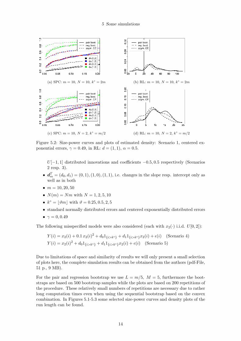
Figure 5.2: Size-power curves and plots of estimated density: Scenario 1, centered ex-ponential errors, γ = 0.49, in RL: d = (1, 1), α = 0.5.

U [−1, 1] distributed innovations and coefficients −0.5, 0.5 respectively (Scenarios2 resp. 3).

• dTm = (d0, d1) = (0, 1), (1, 0), (1, 1), i.e. changes in the slope resp. intercept only aswell as in both

• m = 10, 20, 50

• N(m) = Nm with N = 1, 2, 5, 10

• k◦ = bϑmc with ϑ = 0.25, 0.5, 2, 5

• standard normally distributed errors and centered exponentially distributed errors

• γ = 0, 0.49

The following misspecified models were also considered (each with x2(·) i.i.d. U [0, 2]):

Y (i) = x2(i) + 0.1x2(i)2 + d01{i>k◦} + d11{i>k◦}x2(i) + ε(i) (Scenario 4)

Y (i) = x2(i)2 + d01{i>k◦} + d11{i>k◦}x2(i) + ε(i) (Scenario 5)

Due to limitations of space and similarity of results we will only present a small selectionof plots here, the complete simulation results can be obtained from the authors (pdf-File,51 p., 9 MB).

For the pair and regression bootstrap we use L = m/5, M = 5, furthermore the boot-straps are based on 500 bootstrap samples while the plots are based on 200 repetitions ofthe procedure. These relatively small numbers of repetitions are necessary due to ratherlong computation times even when using the sequential bootstrap based on the convexcombination. In Figures 5.1-5.3 some selected size-power curves and density plots of therun length can be found.

14

5 Some simulations

(a) SPC: Scenario 2 (b) RL: Scenario 2

(c) SPC: Scenario 3 (d) RL: Scenario 3

(e) SPC: Scenario 4 (f) RL: Scenario 4

(g) SPC: Scenario 5 (h) RL: Scenario 5

Figure 5.3: Size-power curves and plots of estimated density: centered exponential errors,γ = 0, m = 10, N = 2, k◦ = m/4, in RL: d = (1, 1), α = 0.5.

15

6 Proofs of Section 3

It can be concluded from the simulations that both bootstrap methods perform betterthan the asymptotic closed-end procedure for two reasons:

• The bootstrap methods hold the level much better.

• The run-time of the bootstrap methods is a bit longer, however a much smallerpercentage of all rejections takes place before the change. This can especially beseen in Figure 5.2 and may be caused partly by the smaller level of the bootstrapmethods.

• All three methods still work well under the misspecified scenarios 3 and 4 (cf.Figure 5.3).

• All three methods become approximately equivalent for m > 50 (for p = 2).

• The bootstrap methods already work well for a very small historic data length ofm = 10 (for p = 2).

Concerning a comparison of the two bootstrap methods the following can be noticed:

• The pair bootstrap holds the level better consequently has a somewhat smallerpower and higher run-length. Interestingly, this remains true even if the regres-sors are correlated (Figure 5.3, Scenarios 2 and 3), where one would expect theregression bootstrap to be better.

• The bootstrap methods become very close for m > 20.


The following lemma summarizes some results on C and c1(m, k, `). It follows immedi-ately from Lemma 5.1 in Horvath et al. [10].

Lemma 6.1. Under the Assumption A.1 (ii) it holds as m→∞

a)∥∥mC−1

m −C−1∥∥∞ = O(m−ρ) P − a.s.

b) sup`>1

supk>1

‖c1(m, k, `)− `c1‖∞(m+ `)1−ρ + `m−ρ

= O(1) P − a.s.

Our aim is to prove that the bootstrap critical values are uniformly asymptoticallycorrect under the null hypothesis and bounded under alternatives (see equations (6.24)resp. (6.25) below).

In view of the following lemma it is clear that for this it is sufficient to prove the correctasymptotic behavior of supk F

(R∗)m,k (x).

Lemma 6.2. Let c, ck(m) be such that P (Y > c) = α respectivelyP ∗m,k(Yk(m) > ck(m)) 6 α for some 0 < α < 1 (ck(m) minimal), where Yk(m) is somestatistic and Y is a random variable with strictly monotone and continuous distributionfunction in a compact neighborhood K of c.

a) Moreover let for all x in K (as m→∞)

sup16k<∞

∣∣P ∗m,k(Yk(m) 6 x)− P (Y 6 x)∣∣→ 0 P − a.s. (6.1)

16


Then, as m→∞,

sup16k<∞

|ck(m)− c| → 0 P − a.s. (6.2)

b) If instead we only have that for each ε > 0 there exists a constant A = A(ε) > 0, s.t.

sup16k<∞

∣∣P ∗m,k(Yk(m) > A)∣∣ 6 ε+ o(1) P − a.s. (6.3)

then

sup16k<∞

|ck(m)| = O(1) P − a.s. (6.4)

Proof. For a) we refer to the proof of Kirch [14], Lemma A.1. Concerning b), con-sider the set of all ω ∈ M with P (M) = 1 and such that (6.3) holds. We prove(6.4) for all ω ∈ M by contradiction. If (6.4) does not hold, we find a subsequenceβ(·) and a function f , such that cf(β(m))(β(m)) → ∞. On the other hand sinceP ∗m,f(β(m))

(Yf(β(m))(m) > cf(β(m))

)6 α we get by the minimality of cf(β(m))(m) by (6.3)

that

cf(β(m))(m) 6 A(α/2),

which is a contradiction.

Note that F (R∗)m,k is determined mainly by the distribution of (` = 1, . . . , N(m))

g(m, `, γ) Γ(m, `, γ)(e∗m,k(1), . . . , e∗m,k(m+ `))

=m+∑i=m+1

em,k(Um,k(i))− c1(m, k, `)TC−1m

m∑j=1

x(j)em,k(Um,k(i))

and the bootstrap variance (3.5). Note that

em,k(i) =e(i)− x(i)TC−1m+k

m+k∑j=1

x(j)e(j)

+ 1{i>m+k◦}x(i)Tdm − 1{k>k◦}x(i)TC−1m+kCk◦,kdm, (6.5)

and for k > k◦

Ck◦,k =m+k∑

i=m+k◦+1

x(i)x(i)T = Ck −Ck◦ .

From this we can decompose g(m, `, γ)Γ(m, `, γ)(e∗m,k(1), . . . , e∗m,k(m+ `)) as follows:

g(m, `, γ) Γ(m, `, γ)(e∗m,k(1), . . . , e∗m,k(m+ `))

= I1(m, k, `) + I2(m, k, `) + I3(m, k, `) + I4(m, k, `) + I5(m, k, `) + I6(m, k, `),

where

I1(m, k, `) =m+∑i=m+1

e(Um,k(i)),

17


I2(m, k, `) = −c1(m, k, `)TC−1m

m∑j=1

x(j)e(Um,k(j)),

I3(m, k, `) =m+∑i=m+1

x(Um,k(i))TC−1m+k

m+k∑j=1

x(j)e(j)− `

m+ k

m+k∑i=1

e(i),

I4(m, k, `) = −c1(m, k, `)TC−1m

m∑j=1

x(j)x(Um,k(j))TC−1m+k

m+k∑v=1

x(v)e(v)+`

m+ k

m+k∑i=1

e(i),

I5(m, k, `) =m+∑i=m+1

(1{Um,k(j)>m+k◦}x(Um,k(j))Tdm − 1{k>k◦}x(Um,k(j))TC−1

m+kCk◦,kdm

)I6(m, k, `) = −c1(m, k, `)TC−1

m

m∑j=1

x(j)(

1{Um,k(j)>m+k◦}x(Um,k(j))Tdm

− 1{k>k◦}x(Um,k(j))TC−1m+kCk◦,kdm

).

In order to prove (6.1) under H0 resp. (6.3) under H1, we show thatg(m, `, γ)Γ(m, `, γ)(e∗m,k(1), . . . , e∗m,k(m+ `)) is asymptotically determined by I1(m, k, `)respectively I2(m, k, `). Precisely, the following lemma shows that Ij(m, k, `), j = 3, 4,converge uniformly to 0 and the terms Ij(m, k, `), j = 5, 6, which are nonzero only underalternatives, are uniformly bounded.

Lemma 6.3. Let (1.1), Assumption A.1, and (2.1) hold true and either H0 or dm =O(1).

a) Then for all ε > 0 it holds:

(i) sup16k<∞

P ∗m,k

(max

16`<N(m)+1

|I3(m, k, `)|g(m, `, γ)

> ε

)→ 0 P − a.s.,

(ii) sup16k<∞

P ∗m,k

(max

16`<N(m)+1

|I4(m, k, `)|g(m, `, γ)

> ε

)→ 0 P − a.s.

b) Under H0 it holds that Ij(m, k, `) = 0, j = 5, 6, under local alternatives, i.e. ifdm = o(1), it holds for all ε > 0 that

(i) sup16k<∞

P ∗m,k

(max

16`<N(m)+1

|I5(m, k, `)|g(m, `, γ)

> ε

)→ 0 P − a.s.,

(ii) sup16k<∞

P ∗m,k

(max

16`<N(m)+1

|I6(m, k, `)|g(m, `, γ)

> ε

)→ 0 P − a.s.

c) For alternatives, for which only dm = O(1), we get only the following weaker asser-tion: For every ε > 0 there exists A > 0 such that

(i) sup16k<∞

P ∗m,k

(max

16`<N(m)+1

|I5(m, k, `)|g(m, `, γ)

> A

)6 ε+ o(1) P − a.s.,

(ii) sup16k<∞

P ∗m,k

(max

16`<N(m)+1

|I6(m, k, `)|g(m, `, γ)

> A

)6 ε+ o(1) P − a.s.

18


Proof. All terms are sums of i.i.d. random vectors. Therefore, it suffices in all cases tocalculate the variance matrices and to apply the Hajek-Renyi or Markov inequality. Bydirect calculations

E∗m,kx(Um,k(i)) =1

m+ k

m+k∑j=1

x(j),

and since

m+k∑j=1

x(j)TC−1m+kx(v) = (1, 0, . . . , 0)x(v) = 1

we obtain

E∗m,k

x(Um,k(i))TC−1m+k

m+k∑j=1

x(j)e(j)

=1

m+ k

m+k∑j=1

e(j),

showing that I3(m, k, `) is centered. Moreover

E∗m,k(x(Um,k(i))x(Um,k(i))T

)=

1m+ k

Cm+k,

hence (by var(Z) 6 E(Z2))

var∗m,k

x(Um,k(i))TC−1m+k

m+k∑j=1

x(j)e(j)

6

1m+ k

m+k∑j=1

x(j)e(j)

T

C−1m+kCm+kC

−1m+k

m+k∑j=1

x(j)e(j)

=

1m+ k

m+k∑j=1

x(j)e(j)

T

C−1m+k

m+k∑j=1

x(j)e(j)

.

Standard decoupling arguments yield

supk>1

1m+ k

∣∣∣∣∣∣m+k∑j=1

x(j)e(j)

∣∣∣∣∣∣ = o(1) P − a.s., (6.6)

since conditioned on {x(·)} the sequence fulfills the Kolmogorov condition for a strongLLN. This together with Lemma 6.1 shows that, as m→∞,

sup16k<∞

1m+ k

m+k∑j=1

x(j)e(j)

T

C−1m+k

m+k∑j=1

x(j)e(j)

= o(1) P − a.s.

Denote

Zm,k(Um,k(j)) = x(Um,k(j))TC−1m+k

m+k∑v=1

x(v)e(v)− 1m+ k

m+k∑j=1

e(j). (6.7)

19


Conditionally {Zm,k(Um,k(j)} are i.i.d. random variable with

E∗m,k Zm,k(Um,k(1)) = 0,

supk

var∗m,k Zm,k(Um,k(1)) = o(1) P − a.s. (6.8)

We start by proving assertion a)(i): For some D1 > 0

g(m, `, γ) >

{D1m

1/2−γ `γ , ` 6 m,

D1m−1/2 `, ` > m,

(6.9)

yielding for some D2 > 0

N(m)∑l=1

1g2(m, `, γ)

6 D−21 m−1+2γ

m∑`=1

1`2γ

+D−21 m

N(m)∑`=m+1

1`2

6 D2. (6.10)

Then, by the Hajek-Renyi inequality for any ε > 0

P ∗m,k

(max

16`<N(m)+1

|I3(m, k, `)|g(m, `, γ)

> ε

)6 ε−2D2 var∗m,k Zm,k(Um,k(1))→ 0 P − a.s.

uniformly in k which finishes the proof of a)(i) by (6.8).

Now we prove a) (ii). Notice that I4(m, k, `) can be expressed as the product of twoterms one of them is (conditionally) nonrandom and depends on ` while the other one is(conditionally) random and does not depend on `. We will make use of this fact, whichis why the proof differs from the one of a)(i). By x(i)TC−1

m

∑mj=1 x(j) = 1 it holds

I4(m, k, `) = −c1(m, k, `)TC−1m

m∑j=1

x(j)Zm,k(Um,k(j)).

Denote by uj the jth unit vector i.e. the p-dimensional vector uj = (u1,j , . . . , up,j)T

with ui,j = 1{i=j}, then by Lemma 6.1 a)

E∗m,k

(√muTj C−1

m

m∑i=1

x(i)Zm,k(Um,k(i))

)2

= var∗m,k

(√m

m∑i=1

uTj C−1m x(i)Zm,k(Um,k(i))

)

=(var∗m,k Zm,k(Um,k(1))

)uTj mC−1

m

m∑i=1

x(i)x(i)T C−1m uj

=(var∗m,k Zm,k(Um,k(1))

)uTj (C−1 + o(1)) uj = o(1) P − a.s. (6.11)

uniformly in k. By Lemma 6.1 b) in addition to (6.9) we additionally get for someD3 > 0

supk>1

sup16`<N(m)+1

∥∥∥∥ c1(m, k, `)T√mg(m, `, γ)

∥∥∥∥∞

6 D3 + o(1) P − a.s. (6.12)

20


Together this yields that

E∗m,k

(max

16`<N(m)+1

|I4(m, k, `)|g(m, `, γ)

)2

= o(1) P − a.s.,

which gives the assertion by the Markov inequality. Now, we prove b) and c). First notethat it suffices to consider k > k◦, since for k 6 k◦ it holds Ij(m, k, `) = 0, j = 5, 6.Denote

Zm,k(Um,k(i)) = 1{Um,k(i)>m+k◦}xT (Um,k(i))dm−1{k>k◦}x

T (Um,k(i))C−1m+kCk◦,kdm.

Direct calculations give

E∗m,k Zm,k(Um,k(i)) = 0,

E∗m,k(Zm,k(Um,k(i))

)2=

1m+ k

dTm(Ck◦,k −Ck◦,kC−1m+kCk◦,k)dm

61

m+ kdTmCk◦,kdm 6

1m+ k

dTmCm+kdm 6 dTmCdm (1 + o(1)) P − a.s. (6.13)

uniformly in k by Lemma 6.1 a).

Assertions b) (i) and c) (i) follow now by the Hajek-Renyi inequality and (6.10).

Furthermore (P − a.s.)

E∗m,k

√muTj C−1m

m∑j=1

x(j)Zm,k(Um,k(j))

2

6 dTmCdm uTj C−1uj (1 + o(1))

(6.14)

uniformly in k. This, in addition to (6.12), yields b) (ii) and c) (ii) by the Markovinequality.

The next lemma allows us to replace I2(m, k, `) by a simpler expression.

Lemma 6.4. Let (1.1), Assumption A.1, and (2.1) hold true. Then for all ε > 0 itholds

sup16k<∞

P ∗m,k

(max

16`<N(m)+1

|I2(m, k, `)− −`m∑m

j=1 e(Um,k(j))|g(m, `, γ)

> ε

)→ 0 P − a.s.

Proof. The proof is a slight modification of Lemma 5.2 in Horvath et al. [10]. Denote

em,k =1

m+ k

m+k∑i=1

e(i), σ2m,k =

1m+ k

m+k∑i=1

(e(i)− em,k)2 . (6.15)

By Assumption A.1 and the law of iterated logarithm we get uniformly in k

supk|m1/2−(ρ−γ)em,k| → 0 P − a.s., sup

k|σ2m,k − σ2| → 0 P − a.s., (6.16)

21


since by assumption ρ− γ > 0 for ρ from Assumption A.1. Let uj denote again the jthunit vector. Then, we get uniformly in k

E∗m,k

(1

m1/2+ρ−γ uTj

m∑i=1

x(i)e(Um,k(i))

)2

=1

m1+2(ρ−γ)

m∑i=1

(uTj x(i))2 var∗ (e(Um,k(1))) +

(uTj

m1/2+ρ−γ

m∑i=1

x(i) E∗(e(Um,k(1))

)2

=1

m1+2(ρ−γ) uTj Cmuj σ2

m,k + (uTj c1 + o(1))2(m1/2−(ρ−γ)em,k

)2

= o(1) P − a.s.(6.17)

By Lemma 6.1 and (6.9) we get

supk

sup16`<N(m)+1

∥∥∥∥c1(m, k, `)T mC−1m − `cT1 C−1

m1/2−ρ+γ g(m, `, γ)

∥∥∥∥∞

= O(1) sup16`<N(m)+1

∣∣∣∣ (m+ `)1−ρ + `m−ρ

m1/2−ρ+γ g(m, `, γ)

∣∣∣∣ = O(1) P − a.s.

Since cT1 C−1∑m

i=1 x(j)e(Um,k(i)) =∑m

i=1 e(Um,k(i)) we obtain the assertion by an ap-plication of the Markov inequality.

We are now ready to state the asymptotics of Γ(m, `, γ)(e∗m,k(1), . . . , e∗m,k(m+ `)).

Lemma 6.5. Let (1.1), Assumption A.1, and (2.1) hold true and either H0 or dm =O(1), N(m) is as in Theorem 2.1. Let σ2

m,k as in (6.15).

a) Under H0 and for local alternatives dm = o(1) it holds

sup16k<N(m)+1

∣∣∣∣∣P ∗m,k(

1σm,k

sup16`<N(m)+1

Γ(m, `, γ)(e∗m,k(1), . . . , e∗m,k(m+ `))g(m, `, γ)

6 x

)

− P

(sup

16k<N(m)+1

|W1(k/m)− k/mW2(1)|(1 + k/m)(k/(k +m))γ

6 x

)∣∣∣∣∣→ 0 P − a.s.

b) Under H1 for every ε > 0 there exists a constant A > 0 such that (P − a.s.)

sup16k<N(m)+1

∣∣∣∣∣P ∗m,k(

1σm,k

sup16`<N(m)+1

Γ(m, `, γ)(e∗m,k(1), . . . , e∗m,k(m+ `))g(m, `, γ)

> A

)∣∣∣∣∣ 6 ε+o(1).

Proof. The proof of Theorem 2.3 in Kirch [14] shows that (note that this correspondsto the null hypothesis there)

sup16k<N(m)+1

∣∣∣∣∣P ∗m,k 1σm,k

sup16`<N(m)+1

∣∣∣∑m+`i=m+1

(e(Um,k(i))− 1

m

∑mj=1 e(Um,k(j))

)∣∣∣g(m, `, γ)

6 x

− P

(sup

16k<N(m)+1

|W1(k/m)− k/mW2(1)|(1 + k/m)(k/(k +m))γ

6 x

)∣∣∣∣∣→ 0 P − a.s.

22


Putting this together with Lemmas 6.3 and 6.4, as well as (6.16) yields the assertion.

Before we finally deal with the bootstrapped variance, we need a small auxiliary lemmawhich will also be crucial for the proof of the pair bootstrap.

Lemma 6.6. Let (1.1) and Assumption A.1 hold true. For any 12 < ξ < 1 and any

ε > 0 (P − a.s.)

a) supk>1

P ∗m,k

(m−ξ

∥∥∥∥∥m∑s=1

x(Um,k(s))T e(Um,k(s))

∥∥∥∥∥∞

> ε

)→ 0

b) supk>1

P ∗m,k

(m−ξ

∥∥∥∥∥m∑s=1

x(Um,k(s))T e(Um,k(s))1{Um,k(s)>m+k◦}

∥∥∥∥∥∞

> ε

)→ 0

If for the pair bootstrap additionally Assumption A.3 holds, then we even get the asser-tions for ξ = 1

2 .

Proof. By the von Bahr-Esseen inequality (cf. Theorem 3 in [17]) with 1/ξ we get forsome constant D > 0 and for any c > 0

supk>1

P ∗m,k

(m−ξ

∥∥∥∥∥m∑s=1

x(Um,k(s))T e(Um,k(s))

∥∥∥∥∥∞

> c

)

6D

c1/ξsupk>1

1m+ k

m+k∑j=1

‖x(i)e(i)‖1/ξ∞ = O(1) P − a.s.,

since conditioned on {x(·)} the sequence fulfills condition (1) in Theorem 5.2.1 in Chowand Teicher [6] similarly to (6.6). This proves a) but b) is analogous.

The same arguments also holds for ξ = 12 if the stronger assumption A.3 holds.

Finally we deal with the bootstrapped variance in the following lemma:

Lemma 6.7. Let (1.1) and Assumption A.1 hold true and either H0 or dm = O(1). Letσ2m,k be as in (6.15).

a) Under H0 or local alternatives (dm = o(1)) it holds for all ε > 0

supkP ∗m,k

∣∣∣∣∣∣ σm,kσ(R∗)m,k

− 1

∣∣∣∣∣∣ > ε

→ 0 P − a.s.

b) Under H1 for every ε > 0 there exists A > 0 such that

supkP ∗m,k

∣∣∣∣∣∣ σm,kσ(R∗)m,k

∣∣∣∣∣∣ > A

6 ε+ o(1) P − a.s.

Proof. By (6.5) it holds

e∗m,k(i)− x(i)TC−1m

m∑j=1

x(j)e∗m,k(j)

= J1(m, k, i) + J2(m, k, i) + J3(m, k, i) + J4(m, k, i) + J5(m, k, i) + J6(m, k, i),

23


where

J1(m, k, i) = e(Um,k(i)),

J2(m, k, i) = −x(i)TC−1m

m∑j=1

x(j)e(Um,k(j)),

J3(m, k, i) = −x(Um,k(i))TC−1m+k

m+k∑j=1

x(j)e(j) + em,k,

J4(m, k, i) = x(i)TC−1m

m∑j=1

x(j)

(x(Um,k(j))TC−1

m+k

m+k∑v=1

x(v)e(v)− em,k

),

J5(m, k, i) = 1{Um,k(i)>m+k◦}x(Um,k(i))Tdm − 1{k>k◦}x(Um,k(i))TC−1m+kCk◦,kdm,

J6(m, k, i) = −x(i)TC−1m

m∑j=1

x(j)x(Um,k(j))T(

1{Um,k(j)>m+k◦} − 1{k>k◦}C−1m+kCk◦,k

)dm,

where em,k is as in (6.15). Note that J5(m, k, i) and J6(m, k, i) are equal to 0 under thenull hypothesis and under alternatives for k 6 k◦.

The following relations hold true for any fixed ε > 0 as m→∞.

By Lemma A.3 and the proof of Theorem 2.3 in Kirch [14] (this corresponds to the nullhypothesis there) it holds

supk>1

P ∗m,k

(∣∣∣∣∣ 1m

∑mi=1(e(Um,k(i))− em,k)2

σ2m,k

− 1

∣∣∣∣∣ > ε

)→ 0 P − a.s.,

which in addition to (6.16) yields

supk>1

P ∗m,k

(∣∣∣∣∣1

m−p∑m

i=1 J21 (m, k, i)

σ2m,k

− 1

∣∣∣∣∣ > ε

)→ 0 P − a.s. (6.18)

Denote by uj again the jth unit vector. By Lemma 6.1 and (6.17) it holds by theCauchy-Schwarz inequality

E∗m,k

(1m

m∑i=1

J22 (m, k, i)

)

= E∗m,k

1m

m∑i=1

x(i)TC−1m

m∑j=1

x(j)e(Um,k(j))

26 p2‖mC−1

m ‖∞ maxj=1,...,p

E∗m,k

(uTjm

m∑i=1

x(i)e(Um,k(i))

)2

→ 0 P − a.s.,

which yields by an application of the Markov inequality

supk>1

P ∗m,k

(1

m− p

m∑i=1

J22 (m, k, i) > ε

)→ 0 P − a.s. (6.19)

24


Noting that J3(m, k, i) = −Zm,k(Um,k(i)) as in the proof of Lemma 6.3, hence by anapplication of the Markov inequality in addition to (6.8)

supk>1

P ∗m,k

(1

m− p

m∑i=1

J23 (m, k, i) > ε

)→ 0 P − a.s. (6.20)

Similarly by (6.11)

supk>1

P ∗m,k

(1

m− p

m∑i=1

J24 (m, k, i) > ε

)

6 supk>1

1ε

E∗m,k

1m− p

m∑j=1

x(j)TZm,k(Um,k(j))C−1m

m∑j=1

x(j)Zm,k(Um,k(j))

6

1ε

∥∥∥∥ 1m

Cm

∥∥∥∥∞

p2

m− psupk>1

supj=1,...,p

E∗m,k

(√muTj C−1

m

m∑v=1

x(v)Zm,k(Um,k(v))

)2

→ 0 P − a.s. (6.21)

Putting (6.18) to (6.20) together with (6.16) yields assertion a) under H0.

Now we prove the assertions under alternatives. First, note that it is sufficient to considerk > k◦, since otherwise J5 and J6 are equal to 0. First we prove that J6 is negligible:By (6.14) it holds

supk>1

P ∗m,k

(1m

m∑i=1

J26 (m, k, i) > ε

)

61ε

p2

m− p

∥∥∥∥ 1m

Cm

∥∥∥∥∞

supj=1,...,p

E∗m,k

√muTj C−1m

m∑j=1

x(j)Zm,k(Um,k(j))

2

= o(1) P − a.s. (6.22)

J5 is only negligible for local alternatives but still bounded for fixed alternatives. Pre-cisely for any c > 0,

supk>1

P ∗m,k

(1m

m∑i=1

J25 (m, k, i) > c

)6dTmCdm

c2+ o(1) P − a.s. (6.23)

by (6.13), since J5(m, k, i) = Zm,k(Um,k(i)) as in the proof of Lemma 6.3. This yields a)under local alternatives.

For fixed alternatives note that

(σ

(R∗)m,k

)2=

1m

m∑i=1

6∑j=1

J2j (m, k, i) +

∑u6=v

Ju(m, k, i)Jv(m, k, i)

.

The square terms are negligible except for J21 and J2

5 by (6.19) – (6.22). By the Cauchy-Schwarz inequality, (6.18) and (6.23) the same holds true for the mixed terms except

25


J1 J5 but the latter one is also negligible due to Lemmas 6.1 and 6.6 since

1m

m∑s=1

(J1(m, k, s)J5(m, k, s)) =1m

m∑s=1

x(Um,k(s))T e(Um,k(s))1{Um,k(s)>m+k◦}dm

− 1m

m∑s=1

x(Um,k(s))T e(Um,k(s))C−1m+kCk◦,kdm.

This shows that the only influential terms are 1m

∑mi=1(J2

1 (m, k, i) + J25 (m, k, i)). But

since σ(R∗)m,k in Lemma 6.6. b) is in the denominator and 1

m

∑mi=1(J2

1 (m, k, i)+J25 (m, k, i)) >

1m

∑mi=1 J

21 (m, k, i) assertion b) follows by (6.18).

Putting the above lemmas together we easily obtain Theorem 3.1.Proof Proof of Theorem 3.1. Putting together Lemmas 6.5 and 6.7 we obtain underH0 as well as local alternatives

sup16k<N(m)+1

∣∣∣∣∣P ∗m,k 1

σ(R∗)m,k

sup16`<N(m)+1

Γ(m, `, γ)(e∗m,k(1), . . . , e∗m,k(m+ `))g(m, `, γ)

6 x

− P

(sup

16k<N(m)+1

|W1(k/m)− k/mW2(1)|(1 + k/m)(k/(k +m))γ

6 x

)∣∣∣∣∣→ 0 P − a.s.

By Lemma 6.2 this yields

supk>1|c(R)m,k − c| → 0 P − a.s., (6.24)

where c is the asymptotic critical value obtained from the distribution of sup06t61− 1N+1

|W (t)|tγ .

Together with Theorem 2.1 this implies a).

Under H1, by Lemmas 6.5 and 6.7 for every ε > 0 there exists a constant A > 0 suchthat (P − a.s.)

sup16k<N(m)+1

∣∣∣∣∣∣P ∗m,k 1

σ(R∗)m,k

sup16`<N(m)+1

Γ(m, `, γ)(e∗m,k(1), . . . , e∗m,k(m+ `))g(m, `, γ)

> A

∣∣∣∣∣∣ 6 ε+o(1)

By Lemma 6.2 this yields

supk>1|c(R)m,k| = O(1) P − a.s. (6.25)

Together with Theorem 2.2 this implies b).


Denote

A1(m, k, `) =m+∑i=m+1

e∗m,k(i)

26


A2(m, k, `) =m+∑i=m+1

x∗m,k(i)

A3(m, k) =m∑j=1

x∗m,k(j)x∗Tm,k(j)

A4(m, k) =m∑s=1

x∗m,k(s)e∗m,k(s)

A5(m, k, `) =m+∑i=m+1

x∗m,k(i)1{Um,k(i)>m+k◦}

A6(m, k) =m∑s=1

x∗m,k(s)x∗Tm,k(s)1{Um,k(s)>m+k◦}

where e∗m,k(i) = e(Um,k(i)), which is different from the bootstrapped residuals in theregression bootstrap. Similarly to (3.1) it holds

g(m, k, γ) Γ(m, `, γ)∗m,k = B1(m, k, `) +B2(m, k, `) +B3(m, k, `) +B4(m, k, `),

where

B1(m, k, `) = A1(m, k, `),

B2(m, k, `) = −AT2 (m, k, `)A−1

3 (m, k)A4(m, k)

B3(m, k, `) =(A5(m, k, `)− `E∗m,k x∗m,k(1)1{Um,k(1)>m+k◦}

)dm,

B4(m, k, `) = −(AT

2 (m, k, `)A−13 (m, k)A6(m, k)− `E∗m,k x∗m,k(1)1{Um,k(1)>m+k◦}

)dm.

The next lemma gives some properties of the terms Aj .

Lemma 7.1. Let (1.1) and Assumption A.1 hold true.

a) Under either Assumption A.2 or A.3 we get for any ε > 0

sup16k<N(m)+1

P ∗m,k

(1

m1−η ‖A3(m, k)−mC‖∞ > ε

)→ 0

P − a.s. for some η > 0.

b) Under either Assumption A.2 or A.3 we get for any ε > 0

sup16k<N(m)+1

P ∗m,k

(∥∥∥∥ 1mA6(m, k)− E∗ x∗m,k(1)x∗m,k(1)T 1{Um,k(i)>m+k◦}

∥∥∥∥∞

> ε

)→ 0 P−a.s.

Proof. First note that from AssumptionsA.1 (ii) we get for every ω ∈M with P (M) = 1the existence of a constant D(ω), such that∥∥∥∥∥

j∑i=1

(x(i)(ω)x(i)T (ω)−C)

∥∥∥∥∥∞

6 D(ω)j−ρ

for each j. Subtracting the term for j and j − 1 we get

‖x(j)(ω)x(j)T (ω)‖∞ 6 ‖C‖∞ + 2D(ω)j1−ρ,

27


which yields

‖x(j)x(j)T ‖∞ = O(j1−ρ) P − a.s. (7.1)

Further note that

E∗m,k(x∗m,k(i)x

∗m,k(i)

T ) =1

m+ k

m+k∑j=1

x(i)x(i)T = C +O(m−ρ) P − a.s. (7.2)

uniformly in k by Assumption A.1. This, (7.1) and an application of the Chebyshevinequality yields now (the square of the matrix is meant componentwise)

sup16k<N(m)+1

P ∗m,k

(1

m1−η

∥∥∥∥∥m∑i=1

(x∗m,k(i)x∗m,k(i)

T −C)

∥∥∥∥∥∞

> ε

)

6 O(m2η−2ρ) +O(1)1

m1−2ηsup

16k<N(m)+1

1m+ k

∥∥∥∥∥m+k∑i=1

(x(i)x(i)T )2∥∥∥∥∥∞

6 O(m2η−2ρ) +O

((m+N(m))1−ρ

m1−2η

)supk>1

supj=1,...,p

1m+ k

m+k∑i=1

x2j (i)

= O(m2η−2ρ +m2η−ε) = o(1) P − a.s.

under Assumption A.2 for some ρ > 0, which yields a). A similar argument but usingA.3 and the von Bahr-Esseen inequaltiy (cf. Theorem 3 in [17]) also yields assertion a).

Analogously we obtain b).

The next lemma is the analogue to Lemmas 6.3 and 6.4 for the regression bootstrap.

Lemma 7.2. Let (1.1), Assumption A.1, and (2.1) hold true and either H0 or dm =O(1).

a) Then for all ε > 0 it holds:

sup16k<N(m)+1

P ∗m,k

(max

16`<N(m)+1

|B2(m, k, `)− −`m∑m

j=1 e∗m,k(j)|

g(m, `, γ)> ε

)→ 0,

b) Under H0 it holds that Bj(m, k, `) = 0, j = 3, 4, under local alternatives, i.e. ifdm = o(1), it holds for all ε > 0 that

(i) sup16k<N(m)+1

P ∗m,k

(max

16`<N(m)+1

|B3(m, k, `)|g(m, `, γ)

> ε

)= o(1) P − a.s.,

(ii) sup16k<N(m)+1

P ∗m,k

(max

16`<N(m)+1

|B4(m, k, `)|g(m, `, γ)

> ε

)= o(1) P − a.s.

c) For fixed alternatives, for which dm = O(1), we get only the following weaker asser-tion: For every ε > 0 there exists A > 0 such that

(i) sup16k<N(m)+1

P ∗m,k

(max

16`<N(m)+1

|B3(m, k, `)|g(m, `, γ)

> A

)6 ε+ o(1) P − a.s.,

(ii) sup16k<N(m)+1

P ∗m,k

(max

16`<N(m)+1

|B4(m, k, `)|g(m, `, γ)

> A

)6 ε+ o(1) P − a.s.

28


Proof.

−B2(m, k, `) = B2,1(m, k, `) +B2,2(m, k, `) +B2,3(m, k, `),

where

B2,1(m, k, `) = (A2(m, k, `)− E∗m,kA2(m, k, `)T )A3(m, k)−1A4(m, k)

B2,2(m, k, `) = E∗m,kAT2 (m, k, `)(E∗m,kA3(m, k))−1A4(m, k)

B2,3(m, k, `)

= E∗m,kAT2 (m, k, `)(E∗m,kA3(m, k))−1(E∗m,kA3(m, k)−A3(m, k))A3(m, k)−1A4(m, k).

Direct calculations give

E∗m,kAT2 (m, k, `)(E∗m,kA3(m, k))−1 =

`

m+ k

m+k∑i=1

x(i)( m

m+ k

m+k∑i=1

x(i)x(i)T)−1

=`

m(1, 0, . . . , 0)T (7.3)

Therefore

B2,2(m, k, `) =`

m

m∑i=1

e∗m,k(i).

By Lemmas 6.6 and 7.1 as well as (7.2) we get for any ε > 0

supk>1

P ∗m,k(mη−1‖A3(m, k)− E∗m,k A3(m, k)‖∞ > ε

)→ 0 P − a.s. (7.4)

supk>1

P ∗m,k

(m1−ξ‖A3(m, k)−1A4(m, k)‖∞ > ε

)→ 0 P − a.s. (7.5)

for some η > 0 and for ξ as in Lemma 7.1.

By (6.9) we get

sup`>1

`

mg(m, `, γ)= O(m−1/2), (7.6)

which together with (7.3), (7.4) and (7.5) yields

sup16k<N(m)+1

P ∗m,k

(max

16`<N(m)+1

|B2,3(m, k, `)|g(m, `, γ)

> ε

)→ 0 P − a.s.

Finally note that by Assumption A.1 (ii)

var∗m,k(x∗m,k(i)) 6

1m+ k

m+k∑i=1

x(i)x(i)T = C + o(1) P − a.s. (7.7)

uniformly in k. An application of the Hajek-Renyi inequality, (6.10) and (7.5) yields

sup16k<N(m)+1

P ∗m,k

(max

16`<N(m)+1

|B2,1(m, k, `)|g(m, `, γ)

> ε

)→ 0 P − a.s.

29


This completes the proof of a).

In the following let D > 0 be some (non-random) constant which can differ in everyoccurrence. Concerning b) and c), first note that by Assumption A.1 we get uniformlyin k > 1∥∥∥var∗m,k(x

∗m,k(i)1{Um,k(i)>m+k◦})

∥∥∥∞

=1

m+ k

∥∥∥∥∥m+k∑

i=m+k◦

x(i)x(i)T∥∥∥∥∥∞

6 D+o(1) P−a.s.

An application of the Hajek-Renyi inequality, (6.10) and Lemma 7.1 yields for any c > 0

sup16k<N(m)+1

P ∗m,k

(max

16`<N(m)+1

|B3(m, k, `)|g(m, `, γ)

> c

)6 D

‖dm‖2∞c2

+ o(1) P − a.s.,

which proves b) (i) and c) (i).

Concerning B4(m, k, `) we need an analogous decomposition as for B2(m, k, `) above.

−B4(m, k, `) = B4,1(m, k, `) +B4,2(m, k, `) +B4,3(m, k, `),

where

B4,1(m, k, `) =(AT

2 (m, k, `)− E∗m,kAT2 (m, k, `)

)A3(m, k)−1A6(m, k)dm

B4,2(m, k, `)

=(E∗m,kA

T2 (m, k, `)(E∗m,kA3(m, k))−1A6(m, k)− `E∗m,k x∗m,k(1)1{Um,k(1)>m+k◦}

)dm

B4,3(m, k, `)

=(E∗m,kA

T2 (m, k, `)(E∗m,kA3(m, k))−1(E∗m,kA3(m, k)−A3(m, k))A3(m, k)−1A6(m, k)

)dm.

Since

E∗m,k x∗m,k(1)x∗m,k(1)T 1{Um,k(1)>m+k◦} =1

m+ k

m+k∑i=m+k◦

x(i)x(i)T 6 D+o(1) P−a.s.

(7.8)

uniformly in k, we obtain from Lemma 7.1 that for each ε > 0 there exists A > 0 suchthat

supk>1

P ∗m,k(‖A3(m, k)−1A6(m, k)‖∞ > A

)6 ε+ o(1) P − a.s. (7.9)

This in addition to an application of the Hajek-Renyi inequality and (6.10) yields forany c > 0

sup16k<N(m)+1

P ∗m,k

(max

16`<N(m)+1

|B4,1(m, k, `)|g(m, `, γ)

> c

)6 D

‖dm‖2∞c2

+ o(1) P − a.s.

By (7.3) we get

B4,2(m, k, `) =`

m

m∑j=1

(x∗m,k(j)T 1{Um,k(j)>m+k◦} − E∗ x∗m,k(j)1{Um,k(j)>m+k◦})dm.

30


An application of the Chebyshev inequality yields for any c > 0

supk>1

P ∗m,k

1√m

∣∣∣∣∣∣m∑j=1

(x∗m,k(j)T 1{Um,k(j)>m+k◦} − E∗ x∗m,k(j)

T 1{Um,k(j)>m+k◦})dm

∣∣∣∣∣∣ > c

6‖dm‖2∞c2

supk>1

1m+ k

∥∥∥∥∥m+k∑

i=m+k◦

x(i)x(i)T∥∥∥∥∥∞

6 D‖dm‖2∞c2

+ o(1) P − a.s.

(7.10)

Together with (7.6) this yields

sup16k<N(m)+1

P ∗m,k

(max

16`<N(m)+1

|B4,2(m, k, `)|g(m, `, γ)

> c

)6 D

‖dm‖2∞c2

+ o(1) P − a.s.

Finally by (7.3)

B4,3(m, k, `) = − `

m

m∑j=1

(x∗m,k(j)T − E∗m,k x∗m,k(j)

T )A3(m, k)−1A6(m, k)dm

By (7.6), (7.9) and an analogous argument to (7.10) using (7.7) we finally obtain

sup16k<N(m)+1

P ∗m,k

(max

16`<N(m)+1

|B4,3(m, k, `)|g(m, `, γ)

> c

)6 ‖C‖∞

‖dm‖2∞c2

+ o(1) P − a.s.,

which completes the proof.

Now, we prove the equivalent of Lemma 6.7.

Lemma 7.3. Let (1.1), Assumption A.1, and either Assumption A.2 or A.3 hold true.Let σ2

m,k be as in (6.15).

a) Under H0 or local alternatives (dm = o(1)) it holds for all ε > 0

supkP ∗m,k

∣∣∣∣∣∣ σm,kσ(P∗)m,k

− 1

∣∣∣∣∣∣ > ε

→ 0 P − a.s.

b) Under H1 with dm = O(1) for every ε > 0 there exists A > 0 such that

supkP ∗m,k

∣∣∣∣∣∣ σm,kσ(P∗)m,k

∣∣∣∣∣∣ > A

6 ε+ o(1) P − a.s.

Proof. Note that

y∗m,k(i)− x∗m,k(i)T

m∑j=1


T

−1m∑l=1

x∗m,k(l)T y∗m,k(l)

= D1(m, k, i) +D2(m, k, i) +D3(m, k, i),

31


where

D1(m, k, i) = e∗m,k(i),

D2(m, k, i) = −x∗Tm,k(i)A3(m, k)−1A4(m, k),

D3(m, k, i) = x∗Tm,k(i)1{Um,k(i)>m+k◦}dm − x∗Tm,k(i)A3(m, k)−1A6(m, k)dm.

By (6.18) it holds (D1(m, k, i) = J1(m, k, i))

supk>1

P ∗m,k

(∣∣∣∣∣1

m−p∑m

i=1D21(m, k, i)

σ2m,k

− 1

∣∣∣∣∣ > ε

)→ 0 P − a.s. (7.11)

Furthermore sincem∑i=1

D22(m, k, i) = A4(m, k)A−1

3 (m, k)A4(m, k),

for every ε > 0 by Lemmas 6.6 and 7.1

supk>1

P ∗m,k

(1

m− p

m∑i=1

D22(m, k, i) > ε

)→ 0 P − a.s. (7.12)

This shows that asymptotically this summand is negligible as is the mixed term of D1

and D2 due to the Cauchy-Schwarz inequality. Since D3 = 0 under H0 this proves a)under H0.

Concerning alternatives it holds

m∑j=1

D23(m, k, i) = dTmA6(m, k)dm − dTmA6(m, k)(A3(m, k))−1A6(m, k)dm,

which implies due to Lemma 7.1 and (7.8) for every c > 0 for some constant D > 0

supk>1

P ∗m,k

(1

m− p

m∑i=1

D23(m, k, i) > c

)6 D

‖dm‖2∞c2

+ o(1) P − a.s. (7.13)

proving a) for local alternatives, since the mixed terms are again negligible due to theCauchy-Schwarz inequality.

Finally for A4(m, k) =∑m

s=1 x∗m,k(s)e∗m,k(s)1{Um,k(s)>m+k◦}

m∑i=1

D1(m, k, i)D3(m, k, i) = A4(m, k)dm −A4(m, k)(A3(m, k))−1A6(m, k)dm,

which is also negligible due to Lemmas 6.6 and 7.1. We can now finish the proof forfixed alternatives analogously to the proof of Lemma 6.7.

Proof Proof of Theorem 4.1. Due to Lemma 7.2 we obtain the analogous assertionfor the pair bootstrap to what is given for the regression bootstrap in Lemma 6.5. Wecan then conclude as in the proof of Theorem 3.1 using Lemma 7.3.

32

References

References

[1] Andreou, E., and Ghysels, E. Monitoring disruptions in financial markets. J. Econometrics,135:77–124, 2006.

[2] Antoch, J., and Huskova, M. Permutation tests for change point analysis. Statist. Probab.Lett., 53:37–46, 2001.

[3] Aue, A., Hormann, S., Horvath, L., and Huskova, M. Sequential testing for the stability ofportfolio betas. 2009. In preparation.

[4] Aue, A., Horvath, L., Huskova, M., and Kokoszka, P. Change-point monitoring in linearmodels. Econometrics Journal, 9:373–403, 2006.

[5] Berkes, I., Horvath, L., Huskova, M., and Steinebach, J. Applications of permutations tothe simulations of critical values. J. Nonparametr. Stat., 16:197–216, 2004.

[6] Chow, Y.S., and Teicher, H. Probability Theory – Independence, Interchangeability, Mar-tingales. Springer, New York, third edition, 1997.

[7] Fried, R., and Imhoff, M. On the online detection of monotonic trends in time series. Biom.J., 46:90–102, 2004.

[8] Good, P. Permutation, Parametric, and Bootstrap Tests of Hypothesis. Springer, New York,third edition, 2005.

[9] Hall, P. and Wilson, S.R. Two guidelines for bootstrap hypothesis testing. Biometrics,47:757–762, 1991.

[10] Horvath, L., Huskova, M., Kokoszka, P., and Steinebach, J. Monitoring changes in linearmodels. J. Statist. Plann. Inference, 126:225–251, 2004.

[11] Huskova, M. Permutation principle and bootstrap in change point analysis. Fields Inst.Commun., 44:273–291, 2004.

[12] Huskova, M. and Koubkova, A. Monitoring jump changes in linear models. J. Statist. Res.,39:59–78, 2005.

[13] Huskova, M. and Koubkova, A. Sequential procedures for detection of changes in autore-gressive sequences. In Huskova, M. and Lachout, P., editors, Proceedings of the PragueStochstics 2006, pages 437–447, 2006.

[14] Kirch, C. Bootstrapping sequential change-point tests. Sequential Anal., 27:330–349, 2008.[15] Koubkova, A. Change detection in the slope parameter of a linear regression model. Tatra

Mt. Math. Publ., 39:245–253, 2008.[16] Steland, A. A bootstrap view on Dickey-Fuller control charts for AR(1) series. Austrian

Journal of Statistics, 35:339–346, 2006.[17] von Bahr, B., and Esseen, C.-G. Inequalities for the rth absolute moment of a sum of

random variables, 1 ≤ r ≤ 2. Ann. Math. Stat., 36:299–303, 1965.

33

bootstrapping sequential change-point tests for linear...

Documents