multihypothesis sequential probability ratio tests-part ii...
TRANSCRIPT
1366 IEEE TRANSACTIONS ON INFORMATION THEORY, VOL. 46, NO. 4, JULY 2000
Multihypothesis Sequential Probability RatioTests—Part II: Accurate Asymptotic Expansions
for the Expected Sample SizeVladimir P. Dragalin, Alexander G. Tartakovsky, and Venugopal V. Veeravalli, Senior Member, IEEE
Abstract—In a companion paper [13], we proved that twospecific constructions of multihypothesis sequential tests, whichwe refer to as Multihypothesis Sequential Probability Ratio Tests(MSPRT’s), are asymptotically optimal as the decision risks (orerror probabilities) go to zero. The MSPRT’s asymptoticallyminimize not only the expected sample size but also any positivemoment of the stopping time distribution, under very generalstatistical models for the observations. In this paper, based onnonlinear renewal theory we find accurate asymptotic approxi-mations (up to a vanishing term) for the expected sample size thattake into account the “overshoot” over the boundaries of decisionstatistics. The approximations are derived for the scenario wherethe hypotheses are simple, the observations are independent andidentically distributed (i.i.d.) according to one of the underlyingdistributions, and the decision risks go to zero. Simulation resultsfor practical examples show that these approximations are fairlyaccurate not only for large but also for moderate sample sizes. Theasymptotic results given here complete the analysis initiated in[4], where first-order asymptotics were obtained for the expectedsample size under a specific restriction on the Kullback–Leiblerdistances between the hypotheses.
Index Terms—Expected sample size, multihypothesis sequentialprobability ratio tests, nonlinear renewal theory, one-sided SPRT.
I. INTRODUCTION
T HE problem of sequential testing of more than two hy-potheses is considerably more difficult than that of testing
two hypotheses. Optimal solutions are, in general, intractable.Hence, research in sequential multihypothesis testing has beendirected toward the study of practical, suboptimal sequentialtests and the evaluation of their asymptotic performance. Atthe same time multihypothesis testing problems are of consid-erable practical importance, and they arise naturally in many
Manuscript received September 1, 1998; revised February 1, 2000. Thiswork was supported in part by the National Science Foundation under GrantNCR-9523967, by the National Institutes of Health under Grant RO1 HL58751,and by the Office of Naval Research under Grants N00014-95-1-0229 andN00014-99-1-0068. The material in this paper was presented in part at theIEEE International Symposium on Information Theory, MIT, Cambridge, MA,August 1998.
V. P. Dragalin is with SmithKline Beecham Pharmaceuticals, Collegeville,PA 19426-0989 USA (e-mail: [email protected]).
A. G. Tartakovsky is with the Center for Applied Mathematical Sciences,University of Southern California, Los Angeles, CA 90089-1113 USA (e-mail:[email protected]).
V. V. Veeravalli is with School of Electrical Engineering and the Depart-ment of Statistical Science, Cornell University, Ithaca, NY 14853 USA (e-mail:[email protected]).
Communicated by U. Madhow, Associate Editor for Detection and Estima-tion.
Publisher Item Identifier S 0018-9448(00)05295-0.
areas of science and engineering. Examples include: target de-tection/recognition in multiple-resolution radar [2], [6], [24],[26] and electrooptic/infrared systems [14], [30], signal acqui-sition in direct-sequence code-division multiple-access systems[37], statistical pattern recognition [17], clinical trials [19], [39],and others [15], [29], [32].
Simple generalizations of the Wald’s binary sequentialprobability ratio test (SPRT), such as a parallel implementationof a set of simple SPRT’s, may be far from optimum inmultihypothesis problems (see [13, Remark 4.4] for details).Nontrivial extensions of the SPRT are needed to approach op-timum performance asymptotically. In a companion paper [13],we introduced two such extensions, which we referred to asMultihypothesis Sequential Probability Ratio Tests (MSPRT’s).The first test, which is motivated by a Bayesian framework,was considered by Baum and Veeravalli [4], [36], Golubev andKhas’minskii [18], Fishman [16], Tartakovsky [31], [32] invarious contexts. The second test which is formed by a specificcombination of one-sided SPRT’s was suggested by Armitage[1], and studied further in [9]–[11], [25], [29]–[38]. A compar-ison of the pros and cons of the two tests was given by us in[13] and is also summarized in Section II. We showed in [13]that both MSPRT’s are asymptotically optimal as the decisionrisks (or the probabilities of error) go to zero. The MSPRT’sasymptotically minimize not only the expected sample size butalso any positive moment of the stopping time distribution,under very general statistical models for the observations. Theasymptotic optimality of the MSPRT’s makes them attractivecandidates for various practical applications as indicated in[13]. It is hence of great interest to analyze the asymptoticperformance of the MSPRT’s.
A particularly effective way to analyze the asymptoticperformance of sequential tests (for simple hypotheses andindependent and identically distributed (i.i.d.) observations) isthrough the application of renewal theory. For the binary SPRT,it is well known that renewal theory is useful in obtainingasymptotically exact expressions for expected sample sizes anderror probabilities (see, e.g., [28]). An approach to applyingrenewal theory techniques to sequential multihypothesis testswas recently given by Baum and Veeravalli [4] in which theystudied the quasi-Bayesian MSPRT. This MSPRT was shown tobe amenable to an asymptotic analysis usingnonlinearrenewaltheory [40], and asymptotic expressions for the expectedsample size and error probabilities were obtained in [4]. Whilethe work in [4] provided a starting point for the asymptotic per-formance analysis of MSPRT’s, two important open problems
0018–9448/00$10.00 © 2000 IEEE
DRAGALIN et al.: MULTIHYPOTHESIS SEQUENTIAL PROBABILITY RATIO TESTS—PART II 1367
remained. First, the asymptotic analysis in [4] was restrictedto the “asymmetric” situation, where for each hypothesis, thehypothesis with minimum Kullback–Leibler distance amongthe remaining hypotheses is unique. Second, only first-orderasymptotic expressions were obtained for the expected samplesize. These first-order asymptotics were shown to be quiteinaccurate for moderate sample sizes, particularly in the caseof symmetric hypotheses.
In the present paper, we complete the asymptotic analysisinitiated in [4] by addressing both open problems discussedabove. The asymptotic expansions for the expected samplesize are obtained using nonlinear renewal theory (see, e.g.,Lai and Siegmund [21], [22], Siegmund [28], Woodroofe [40],and Zhang [41]). We consider the asymmetric case first, andderive an asymptotically exact expression for the expectedsample size under the assumption that the second momentsof the log-likelihood ratios between the hypotheses are finite.Then, we go on to tackle the general case where the hypothesiswith minimum Kullback–Leibler distance to the hypothesisunder consideration is not necessarily unique. In the generalcase, a much stronger Cramér-type condition is required onthe log-likelihood functions of the observations. Finally, wepresent simulation results for practical examples to show thatthese approximations for the expected sample size are fairlyaccurate not only for large but also for moderate sample sizes.
II. PRELIMINARIES
Let be a sequence of independentand identically distributed (i.i.d.) random variables (generallyvector-valued, ), and letbe their common probability distribution with the densitywith respect to some sigma-finite measure. Our goal is to testsequentially the hypotheses
where are given probability densities.A sequential test is a pair , where is a Markov
(stopping) time and is a terminal decisionfunction taking values in the set . That is,
implies that the decision is in favor of hypothesis
accepts
For each , assume that the consequenceof deciding when is the true hypothesis is given by theloss function . Also, without loss of generality,set the losses due to correct decisions to zero .Then the risk associated with making the decision is givenby
where is the prior probability of the hypothesis, and is the probability of deciding
conditioned on being the true hypothesis. The Bayes riskassociated with the testis the sum .
Note that for the special case of azero–oneloss function,where for , the risk is the same as thefrequentisterror probability , which is defined to be the prob-ability of deciding incorrectly. That is, for the zero–one lossfunction
As in [13], we use to denote the log-likelihood functionsand ratios corresponding to individual observations, i.e.,
and (2.1)
Furthermore, we use to denote the log-likelihood functionsand ratios corresponding to sequence of observations up to agiven time , i.e.,
and (2.2)
Also, for convenience, define the parameters by
(2.3)
We now introduce the two constructions of multihypothesissequential tests, which we refer to as MSPRT’s, whose asymp-totic performance we study in this paper.
Test : Introduce the Markov times
(2.4)
where are positive thresholds . Then the testprocedure has stopping time and terminal de-cision that are given by
if
This test is motivated by a Bayesian framework, and was consid-ered earlier by Golubev and Khas’minskii [18], Fishman [16],Sosulin and Fishman [29], Tartakovsky [31], [32], Baum andVeeravalli [4], [36]. Indeed, for the zero–one loss function, thestopping times may be rewritten as
where
and where
1368 IEEE TRANSACTIONS ON INFORMATION THEORY, VOL. 46, NO. 4, JULY 2000
is thea posterioriprobability of the hypothesis . Note alsothat if (does not depend on), the stopping time of thetest is defined by
where
i.e., we stop as soon as the largest posterior probability exceedsa threshold.
Test : Let
(2.5)be the Markov “accepting” time for the hypothesis, whereare positive thresholds . The testis defined as follows:
if
This test represents a modification of the matrix SPRT (thecombination of one-sided SPRT’s) that was suggested byLorden [25]. It was considered earlier by Armitage [1], Lorden[25], Dragalin [9]–[11], Verdenskaya and Tartakovskii [38],Tartakovsky [32]–[34]. For the zero–one loss function, thestopping times may be rewritten as
where
i.e., is the generalized weighted likelihood ratio betweenand the remaining hypotheses.
It is easy to see that both tests coincide with the Wald’s SPRTin the binary case where . If the distributions of the obser-vations come from exponential families, which are good modelsfor many applications, then has an advantage over in thatit does not require exponential transformations of the observa-tions. This fact makes it more convenient for practical realiza-tion and simulation. Furthermore, may easily be modified tomeet constraints on conditional risks (see [9]–[11], [32]–[34])that may be more relevant in some practical applications. How-ever, as we shall see in the following section,has the advan-tage that it is easier to design the thresholds to preciselymeet constraints on the risks .
In [13], we established that if
(2.6)
then both tests and asymptotically minimize any positivemoment of the stopping time distribution in the class of tests
(sequential and nonsequential) for whichas . Here is a predefined bound on therisk of choosing hypothesis . Furthermore, it follows from[13, Lemma 2.1 and Theorem 4.1] that if ,
, the ratios are bounded
away from zero and infinity, and the condition (2.6) holds, thenfor
as (2.7)
where is the minimum Kullback–Leibler distance between and other hypotheses. Here andin what follows the notation as means that
.Also regardless of the class , if the condition (2.6) holds
and , , then the following first-order approximations for the expected sample size hold [13]:
(2.8)
These asymptotic formulas describe the behavior only of thefirst term of the expansion for the average sample size (ASS).The behavior of the second term remains to be determined.Simulation results given in Section IV show that the first-orderapproximations are usually inaccurate for moderate values ofthresholds which are of main interest in practice. In this paper,we derive higher order approximations to the ASS up to a van-ishing term. As we shall see, in a specific asymmetric case thesecond term is of the order of (i.e., a constant), but in gen-eral it goes to infinity as the square root of the threshold.
It is worth mentioning that one can construct many other “rea-sonable” tests that are asymptotically optimal in the sense (2.7)and, hence, are competitive with the proposed tests. One inter-esting example is therejectingsequential test considered in [34].However, not all reasonable tests are asymptotically optimal.For example, a maximum-likelihood test, which is a direct gen-eralization of the binary SPRT, is not optimum even asymptot-ically if (see [13, Remark 4.4]). At the same time thistest also coincides with SPRT, and is hence an optimal test, when
.
III. A CCURATEASYMPTOTICAPPROXIMATION FOR THEASS
In this section, we obtain asymptotic expansions for the ASSof the tests up to a vanishing term using nonlinear renewaltheory. See, e.g., Lai and Siegmund [21], [22], Siegmund [28],Woodroofe [40], Zhang [41], for detailed discussions of thenonlinear renewal theory results used in this paper.
A. The Asymmetric Case
First we consider the asymmetric case studied in [4] and[36], where the hypothesis for which the Kull-back–Leibler distance, , attains its minimum(over ) is unique. (The reader is reminded of the definitionof and given in (2.1) and (2.2).) Specifically,throughout Section III-A we assume that the following condi-tion holds:
is unique for any
(3.1)
DRAGALIN et al.: MULTIHYPOTHESIS SEQUENTIAL PROBABILITY RATIO TESTS—PART II 1369
In order to apply relevant results from nonlinear renewaltheory, we rewrite the stopping times of (2.4) and (2.5) in theform of a random walk crossing a constant boundary plus anonlinear term that is “slowly changing” in the sense definedin Definition 3.1. By subtracting from both sides of theinequalities in (2.4) and (2.5), we see that
(3.2)
and
(3.3)
where and are defined by
(3.4)
(3.5)
Definition 3.1: The process is said to beslowlychangingif the following two conditions hold:
i) as
in probability (3.6)
ii) for every and some
(3.7)
i.e., is uniformly continuous in probability [40].
Lemma 3.1:Let the condition (3.1) be fulfilled andfor all and . Then the processes
and are slowly changing under
Proof: It is easy to see that
We denote this difference by . We can then rewrite of(3.4) as
where
is a zero-mean random walk with respect to. By the stronglaw of large numbers —a.s. and
w.p. 1 as (3.8)
which implies (3.6) and (3.7). Evidently,
and hence, by a standard sandwich argument, the processis also slowly changing.
An important consequence of the slowly changing propertyis that limiting distributions of the overshoot of a random walk(with positive mean) over a fixed threshold are unchanged by theaddition of a slowly changing nonlinear term (see Woodroofe[40, Theorem 4.1]). In particular, suppose we define the stop-ping time
which corresponds to the one-sided SPRT which tests the hy-pothesis against the closest one . Now let
denote the overshoot at the stopping time. Furthermore, let
denote the limiting distribution of the overshoot.Now, let be a slowly changing process and consider the
stopping time
Then, by [40, Theorem 4.1], the overshoot at the stopping time
has the same limiting distribution as , i.e.,
Now note that from (3.2)
on (3.9)
where is the overshoot of the process overthe level at time . Taking the expectations in both sides ofthis last equality and applying the Wald identity [28], we obtain
(3.10)
A similar equality is true for the Markov time . Indeed, from(3.3)
on (3.11)
where is the overshoot of the process overthe level at time . Applying Wald’s identity, we get
(3.12)
We are now in a position to understand the role of Lemma 3.1.The key point is that since the sequences andare slowly changing, the overshoots and have the samelimiting distributions as (when , , and tend to in-finity). Furthermore, both and converge to the con-stant as . Thus for large and , the ASS’s
and should be approximately equal to
and
1370 IEEE TRANSACTIONS ON INFORMATION THEORY, VOL. 46, NO. 4, JULY 2000
respectively, where
is the expected limiting overshoot. The following theorem is aformal statement of this result and is proved in the Appendix.
Theorem 3.1:Suppose that the condition (3.1) holds andare bounded away from zero and infinity, i.e., as
and
where (3.13)
In addition, assume that and the are-nonarithmetic.1 Then
as
(3.14)
as
(3.15)
Remark 3.1:The condition that are -nonarithmeticis imposed due to the necessity of considering certain discretecases separately in the renewal theorem (see, e.g., Woodroofe[40, Section 2.1]). If are -arithmetic with span ,the results of Theorem 3.1 (as well as of Theorem 3.3 below)hold true as and through multi-ples of (i.e., ) and with respective modifica-tion of definition of .
We note that in the definitions of and of (2.4) and(2.5), and in Theorem 3.1 above, the numbers may beassumed to be arbitrary positive constants not necessarily equalto as we defined them before in (2.3). However,by setting as specified in (2.3), we can precisely control therisks corresponding to the tests and . Now let
Recall that is the limiting distribution of the overshootin the one-sided SPRT as (under the measure ).
The following theorem provides asymptotic expressions for therisks in terms of . Its proof is given in the Appendix.
Theorem 3.2:Let
be the risk of deciding . If we set ,then under the same conditions as in Theorem 3.1
as (3.16)
as (3.17)
1A random variableX is called arithmetic (has arithmetic distribution withspand) if d�X is integer-valued for some nonzero constantd. A typical exampleis the Bernoulli sequence. Otherwise,X is called nonarithmetic (or nonlattice),i.e.,P (X = dm for somem) < 1.
As a consequence of Theorem 3.1 and Theorem 3.2 we havethe following important result.
Corollary 3.1: If
and
then as
(3.18)
(3.19)
(3.20)
It is important to emphasize that the testperforms betterthan the test . Indeed, according to (3.19) and (3.20) the differ-ence between and is equal toif we take . For large the differ-ence may appear to be substantial. However, for the procedurewe guarantee only the inequality while for the pro-cedure the corresponding equality holds. Thus the real differ-ence between the two tests would be less thanif the thresholds can be chosen so thatas . In that case, the difference between andcan be made negligible. For the symmetric case with respect todecision risks, where for all
as (3.21)
the fact that may be implicitly derivedfrom the results of Lorden [25]. More specifically, if
and (3.21) is fulfilled, then
as (3.22)
We suspect that the same result is true as long asare arbi-trary numbers bounded away fromand . We do not have arigorous proof for this case; however, simulation results givenin Section IV agree with this conjecture.
B. The General Case
Thus far we have assumed that the minimum distanceis achieved uniquely (see the condition (3.1)). We
now relax this condition. For fixed, let
be the ordered values of . Through-out the rest of this section we assume that
for some
(3.23)
Note that condition (3.23) includes the fully symmetric situation
for all (3.24)
DRAGALIN et al.: MULTIHYPOTHESIS SEQUENTIAL PROBABILITY RATIO TESTS—PART II 1371
when , and “ ” denotes exclusion of “” from theset. Note also that the previous asymmetric case is covered bysetting .
The derivation of the asymptotics for the general case is morecomplicated than in the asymmetric case. The reason is that ifwe write the Markov times and in the form given in (3.2)and (3.3), the sequences corresponding to andare not necessarily slowly changing in the general case. A dif-ferent approach and stronger conditions (see the Cramér-typecondition (3.31) below) are required to tackle this general case.
Recall that is the log-likelihoodfunction of the observations up to time. Now, let
denote the corresponding mean value of the increment of thelog-likelihood function under .
Let be the ordered values of, with denoting the index of the ordered values,
i.e.,
if (3.25)
with an arbitrary index assignment in case of ties.Now, under assumption (3.23), there arevalues that achieve
the minimum distance . Since , we musthave values that achieve the maximum of , i.e.,
Next, define an-dimensional vectorwith components
Obviously, is zero-mean. Let denote itscovariance matrix with respect to .
Now let
be the density of a multivariate normal distribution function withcovariance matrix .
The asymptotic expansions in the general case are derivedusing normal approximations (see Bhattacharya and Rao [5]). Inthis context, we introduce the variables and . The vari-able is the expected value of the maximum ofzero-meannormal random variables with the density function , i.e.,
(3.26)
and is given by
(3.27)where
(3.28)
and where is a polynomial in of degree whosecoefficients involve and the -cumulants of up to order
and is given explicitly by Bhattacharya and Rao in [5, formula(7.19) ]. Due to the lengthiness of this formula we have not in-cluded it here. Computing the constant for a given appli-cation is relatively straightforward, since the integral in (3.26)involves only the covariance matrix of the vector; furthersimplification results in the case where is diagonal. Com-puting the constant is, in general, quite difficult due to thefact that the polynomial is a complicated function of thecumulants of . However, in the symmetric situation (which isusually of interest), where is of the form (with beingthe identity matrix), and , for , a con-siderable simplification is possible (see Section III-C2 below).Note that the application of the normal approximations requiresa Cramér-type condition on the joint characteristic function ofthe vector given in (3.31) below.
We now present a “heuristic” outline of our approach tofinding asymptotics in the general case. We focus on the secondtest , since our approach works more naturally for this test.As we shall see in the proof of Theorem 3.3, the asymptoticASS results for the follow from those for .
The Markov time of (2.5) may be written in the form
(3.29)
where
is a random walk with increments having positive mean, and
It is established in the proof of Theorem 3.3 that is aslowly changing sequence that converges in distribution to arandom variable , and that
as
where is defined in (3.27). In comparing with the corre-sponding equation for the asymmetric case given in (3.3), wesee that is written in terms of the log-likelihood functionof the observations under as opposed to the log-likelihoodratios. Defining in this fashion is required for the corre-sponding sequence to be slowly changing in the generalcase. Also note that in addition to the slowly changing term thereis a nonlinear deterministic term that is added to the thresholdin (3.29).
Now note that from (3.29)
on (3.30)
where is the overshoot of the processover the level at time . In the limit as , we expect
to approximately satisfy the equation
where is the limiting overshoot. Solving this equation forgives
1372 IEEE TRANSACTIONS ON INFORMATION THEORY, VOL. 46, NO. 4, JULY 2000
Finally, using uniform integrability arguments, we expect that
where is the expected limiting overshoot, and is expec-tation of the limit of the slowly changing sequence . Thefollowing theorem formalizes this result, and the detailed proofbased on the renewal theory of Zhang [41] is given in the Ap-pendix. We write and for brevity.
Theorem 3.3:Suppose that is -nonarithmetic, thecovariance matrix of the vector is positive-definite,
, the condition (3.13) holds, and the Cramércondition
(3.31)
on the joint characteristic function of is satisfied. Then
as (3.32)
as (3.33)
where is a constant which does not dependon , and is the expectation of the limiting overshoot in theone-sided SPRT based on the log-likelihood ratio
Remark 3.2:Numerical results given in Section IV indicatethat setting in (3.33) consistently produces the bestmatch with simulated ASS values for test.
Remark 3.3:We note that in the general case we have notbeen able to obtain the counterpart of Theorem 3.2. Thus weneed to rely on weaker Wald-type inequalities for the risks inorder to set the thresholds to meet risk constraints. In particular,as we established in [13, Lemma 2.1]
(3.34)
C. Some Special Cases
In the following we address the issue of computing the con-stants and appearing in asymptotic expansions for theASS given in Theorem 3.3.
1) Case 1: In the asymmetric case (3.1), , and it iseasily shown that . Also, as shown in [5, eq. (7.21)],
in this case. Now, since for the stan-dard Gaussian random variable , we see from(3.27) that . Thus the resulting expression forthe ASS is consistent with the result of Theorem 3.1.
2) Case 2: Consider the symmetric case whereare identically distributed (but not necessarily inde-
pendent), and where is of the form (with being
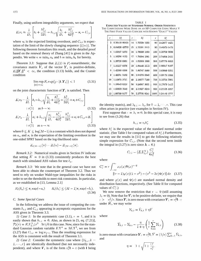
TABLE IEXPECTED VALUES OF STANDARD NORMAL ORDER STATISTICS
THE COMPUTATIONS WERE DONE ON AN HP COMPUTERUSING MAPLE VTHE FIRST FOUR VALUES COINCIDE WITH KNOWN “EXACT” V ALUES
the identity matrix), and , for . This caseoften arises in practice (see examples in Section IV).
First suppose that . In this special case, it is easyto see from (3.26) that
(3.35)
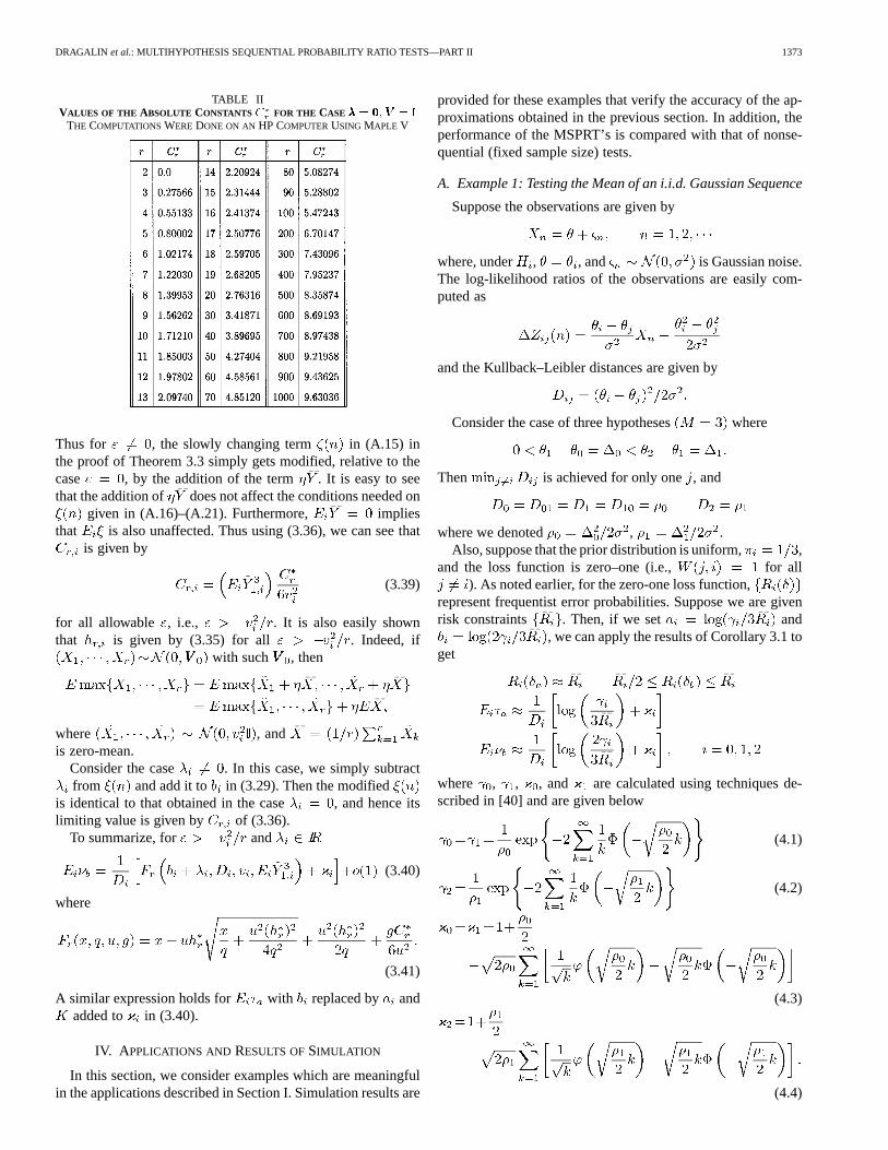
where is the expected value of the standard normal orderstatistic. (See Table I for computed values of.) Furthermore,we may use the results in [11] to get the following relativelysimple expression for . (Note that the second term insidethe integral in (3.27) is zero since .)
(3.36)
where
(3.37)
and where and are standard normal density anddistribution functions, respectively. (See Table II for computedvalues of .)
We now remove the restriction that (still assuming). Note that for to be positive-definite, we require that
. Since is zero mean with covarianceunder , we may write
where
(3.38)
is zero-mean with covariance ,and
DRAGALIN et al.: MULTIHYPOTHESIS SEQUENTIAL PROBABILITY RATIO TESTS—PART II 1373
TABLE IIVALUES OF THE ABSOLUTE CONSTANTS C FOR THE CASE ��� = 000; VVV =
THE COMPUTATIONSWEREDONE ON AN HP COMPUTERUSING MAPLE V
Thus for , the slowly changing term in (A.15) inthe proof of Theorem 3.3 simply gets modified, relative to thecase , by the addition of the term . It is easy to seethat the addition of does not affect the conditions needed on
given in (A.16)–(A.21). Furthermore, impliesthat is also unaffected. Thus using (3.36), we can see that
is given by
(3.39)
for all allowable , i.e., . It is also easily shownthat is given by (3.35) for all . Indeed, if
with such , then
where , andis zero-mean.
Consider the case . In this case, we simply subtractfrom and add it to in (3.29). Then the modified
is identical to that obtained in the case , and hence itslimiting value is given by of (3.36).
To summarize, for and
(3.40)
where
(3.41)
A similar expression holds for with replaced by andadded to in (3.40).
IV. A PPLICATIONS AND RESULTS OFSIMULATION
In this section, we consider examples which are meaningfulin the applications described in Section I. Simulation results are
provided for these examples that verify the accuracy of the ap-proximations obtained in the previous section. In addition, theperformance of the MSPRT’s is compared with that of nonse-quential (fixed sample size) tests.
A. Example 1: Testing the Mean of an i.i.d. Gaussian Sequence
Suppose the observations are given by
where, under , , and is Gaussian noise.The log-likelihood ratios of the observations are easily com-puted as
and the Kullback–Leibler distances are given by
Consider the case of three hypotheses where
Then is achieved for only one, and
where we denoted , .Also, suppose that the prior distribution is uniform, ,
and the loss function is zero–one (i.e., for all). As noted earlier, for the zero-one loss function,
represent frequentist error probabilities. Suppose we are givenrisk constraints . Then, if we set and
, we can apply the results of Corollary 3.1 toget
where , , , and are calculated using techniques de-scribed in [40] and are given below
(4.1)
(4.2)
(4.3)
(4.4)
1374 IEEE TRANSACTIONS ON INFORMATION THEORY, VOL. 46, NO. 4, JULY 2000
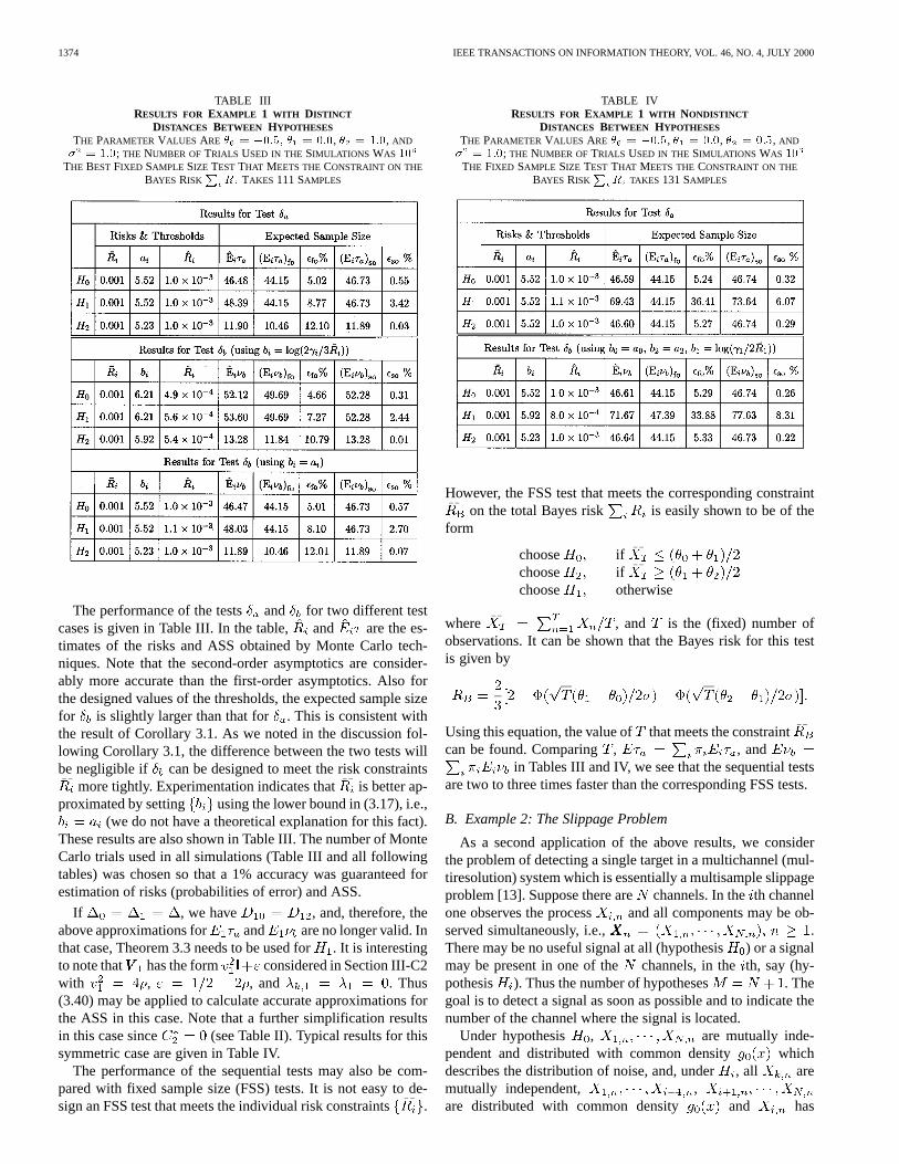
TABLE IIIRESULTS FOR EXAMPLE 1 WITH DISTINCT
DISTANCES BETWEEN HYPOTHESESTHE PARAMETER VALUES ARE � = �0:5; � = 0:0, � = 1:0, AND
� = 1:0; THE NUMBER OF TRIALS USED IN THE SIMULATIONS WAS 10
THE BEST FIXED SAMPLE SIZE TEST THAT MEETS THECONSTRAINT ON THE
BAYES RISK R TAKES 111 SAMPLES
The performance of the tests and for two different testcases is given in Table III. In the table, and are the es-timates of the risks and ASS obtained by Monte Carlo tech-niques. Note that the second-order asymptotics are consider-ably more accurate than the first-order asymptotics. Also forthe designed values of the thresholds, the expected sample sizefor is slightly larger than that for . This is consistent withthe result of Corollary 3.1. As we noted in the discussion fol-lowing Corollary 3.1, the difference between the two tests willbe negligible if can be designed to meet the risk constraints
more tightly. Experimentation indicates that is better ap-proximated by setting using the lower bound in (3.17), i.e.,
(we do not have a theoretical explanation for this fact).These results are also shown in Table III. The number of MonteCarlo trials used in all simulations (Table III and all followingtables) was chosen so that a 1% accuracy was guaranteed forestimation of risks (probabilities of error) and ASS.
If , we have , and, therefore, theabove approximations for and are no longer valid. Inthat case, Theorem 3.3 needs to be used for. It is interestingto note that has the form considered in Section III-C2with , , and . Thus(3.40) may be applied to calculate accurate approximations forthe ASS in this case. Note that a further simplification resultsin this case since (see Table II). Typical results for thissymmetric case are given in Table IV.
The performance of the sequential tests may also be com-pared with fixed sample size (FSS) tests. It is not easy to de-sign an FSS test that meets the individual risk constraints.
TABLE IVRESULTS FOR EXAMPLE 1 WITH NONDISTINCT
DISTANCES BETWEEN HYPOTHESESTHE PARAMETER VALUES ARE � = �0:5, � = 0:0, � = 0:5, AND
� = 1:0; THE NUMBER OF TRIALS USED IN THE SIMULATIONS WAS 10
THE FIXED SAMPLE SIZE TEST THAT MEETS THECONSTRAINT ON THE
BAYES RISK R TAKES 131 SAMPLES
However, the FSS test that meets the corresponding constrainton the total Bayes risk is easily shown to be of the
form
choose ifchoose ifchoose otherwise
where , and is the (fixed) number ofobservations. It can be shown that the Bayes risk for this testis given by
Using this equation, the value ofthat meets the constraintcan be found. Comparing, , and
in Tables III and IV, we see that the sequential testsare two to three times faster than the corresponding FSS tests.
B. Example 2: The Slippage Problem
As a second application of the above results, we considerthe problem of detecting a single target in a multichannel (mul-tiresolution) system which is essentially a multisample slippageproblem [13]. Suppose there arechannels. In theth channelone observes the process and all components may be ob-served simultaneously, i.e., .There may be no useful signal at all (hypothesis) or a signalmay be present in one of the channels, in theth, say (hy-pothesis ). Thus the number of hypotheses . Thegoal is to detect a signal as soon as possible and to indicate thenumber of the channel where the signal is located.
Under hypothesis , are mutually inde-pendent and distributed with common density whichdescribes the distribution of noise, and, under, all aremutually independent, ,are distributed with common density and has
DRAGALIN et al.: MULTIHYPOTHESIS SEQUENTIAL PROBABILITY RATIO TESTS—PART II 1375
density . The latter describes the distribution of a mixtureof signal and noise.
Assume, for simplicity, that .In other words, the statistical properties of the observed data donot depend on the number of the channel where the signal islocated. Then
(4.5)
Therefore, the log-likelihood ratios are given by
By the symmetry of the problem, the distances(say) are the same for , and so are (say)where
and (4.6)
Also the distances between the nonnull hypotheses are givenby , . Hence , ,
. This means that for hypothesis , we have thefully symmetric case with
; while for any other hypothesis , , theasymmetric condition (3.1) holds with .
Further, we assume that the conditional prior distribution ofthe signal location is uniform, i.e.,
is incorrect
In other words, if is the prior probability of signalabsence, then
Finally, given the symmetry of the problem, the followingthree-valued loss function is appropriate:
forforforotherwise
That is, we assume that the losses associated with false alarms,missing the signal and choosing the wrong signal are, respec-tively, given by , , and . The decision risks are thengiven by
Under these assumptions, it is clear that we require to specifyonly two thresholds for each sequential test, and
. Then, by symmetry, the conditionalerror probabilities for both tests satisfy the following properties:
s.t.
and
Thus we have
To meet constraints , we set
and
for
Then, by Corollary 3.1, we get
(4.7)For hypothesis , we may use the bounds given in (3.34) toset and and thus guar-antee that the risk constraint is met. However, as we seein numerical results, setting , ,
, and result in tests that ap-proximate more accurately (of course, without the guaranteeof being below ).
To compute the expected sample sizes, for , we applyTheorem 3.1 to get
(4.8)
where
To compute the ASS under , we need to use Theorem 3.3.By the symmetry of the problem, in this case. In order tocompute the constants and , it is convenient to use themeasure
as the dominating measure for defining densities. Then the like-lihood functions of (4.5) get modified to
1376 IEEE TRANSACTIONS ON INFORMATION THEORY, VOL. 46, NO. 4, JULY 2000
With these likelihood functions, the vector has componentsgiven by
It is easy to show that the covariance matrix has the form, considered in Section III–C2, where
with being the variance relative to the density function, and where
Furthermore,
Thus (3.40) may be applied to get
(4.9)
(4.10)
where , and is as defined in (3.41).
Special Case: Signal Always PresentWe now consider the situation where the null hypothesisis
excluded from consideration, i.e., we are certain that the signalis present in the system and only its location is to be determined.In this case, we have a fully symmetric set ofhypotheses.
It is easy to see that the distances between the hypotheses arefor all , where and
are as defined in (4.6).Due to the symmetry, one may set , ,
for , and assume a zero–one loss function. Therisks are then all equal
where is the probability ofsignal mixing. In order to meet a risk constraint, we usethe bounds given in (3.34) to set and
. This will guarantee that the con-straint is met. However, as seen in numerical results, setting
and (where )results in tests that approximatemore accurately.
To compute the ASS under any of the hypotheses, say, wefirst note that we have a situation covered under Theorem 3.3with . In order to compute the required constants, itis convenient to use the measure as thedominating measure for defining densities. Then the likelihoodfunctions are given by
The components of the vector are obviously i.i.d. in thiscase, with variance given by
where denotes the variance relative to the density func-tion . Thus . Furthermore, by symmetry,
. Applying (3.40), we get, for all
(4.11)
(4.12)
Here , and is as definedin (3.41).
1) Detection of Deterministic Signals in White GaussianNoise: Consider the problem of detection of a deterministicpulse signal in an -channel radar in the presence of additivewhite Gaussian noise. The pre-processing scheme consists of amatched filter, matched to the pulse. Then the hypotheses are
for
for
where are i.i.d. Gaussian variables (bothandare assumed to be known). Note that
Let denote the signal-to-noise ratio (SNR). Thenit is easy to show that and of (4.6) are both equal to.The constants and are obtained by substi-tuting in (4.1) and (4.3), respectively. The vectoris Gaussian and zero mean. From (3.38), it is clear thatisGaussian and zero-mean as well. Hence . The con-stant can be shown to equal . Using these constants, wecan compute the ASS for both tests for any given costs, priors,and risk constraints. Sample results are given in Table V. Notethat the second-order asymptotics are considerably more accu-rate than the first-order asymptotics, particularly for hypothesis
.In the completely symmetric case (signal is always present
but its location is unknown), the required constants are given by, , , and and are obtained
by substituting in (4.1) and (4.3), respectively.For the completely symmetric case, the best FSS test choosesif , where
and is the (fixed) number of observations. It can be shownthat the risk for this test is given by
Using this equation, the value of that meets the constraintcan be found. Comparing, , and in Table VI, we seethat the sequential tests are usually about two times faster thanthe FSS test.
2) Detection of Fluctuating Signals:Now suppose that onewants to detect a fluctuating signal in additive white Gaussiannoise from data at the output of a pre-processing scheme which
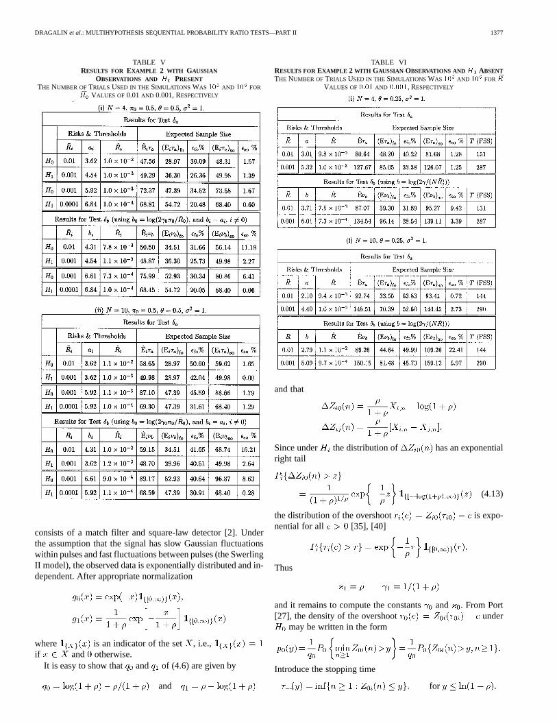
DRAGALIN et al.: MULTIHYPOTHESIS SEQUENTIAL PROBABILITY RATIO TESTS—PART II 1377
TABLE VRESULTS FOR EXAMPLE 2 WITH GAUSSIAN
OBSERVATIONS AND H PRESENTTHE NUMBER OF TRIALS USED IN THE SIMULATIONS WAS 10 AND 10 FOR
�R VALUES OF 0.01AND 0.001, RESPECTIVELY
consists of a match filter and square-law detector [2]. Underthe assumption that the signal has slow Gaussian fluctuationswithin pulses and fast fluctuations between pulses (the SwerlingII model), the observed data is exponentially distributed and in-dependent. After appropriate normalization
where is an indicator of the set , i.e.,if and otherwise.
It is easy to show that and of (4.6) are given by
and
TABLE VIRESULTS FOR EXAMPLE 2 WITH GAUSSIAN OBSERVATIONS AND H ABSENTTHE NUMBER OFTRIALS USED IN THESIMULATIONS WAS 10 AND 10 FOR �R
VALUES OF0:01 AND 0:001, RESPECTIVELY
and that
Since under the distribution of has an exponentialright tail
(4.13)
the distribution of the overshoot is expo-nential for all [35], [40]
Thus
and it remains to compute the constantsand . From Port[27], the density of the overshoot under
may be written in the form
Introduce the stopping time
for
1378 IEEE TRANSACTIONS ON INFORMATION THEORY, VOL. 46, NO. 4, JULY 2000
Obviously,
where . It follows from (4.13) that for any
and hence
Using this last expression we finally obtain
The constant is given by
It is easy to show that
Now, starting with the definition of given in (3.38), a seriesof straightforward calculations leads to
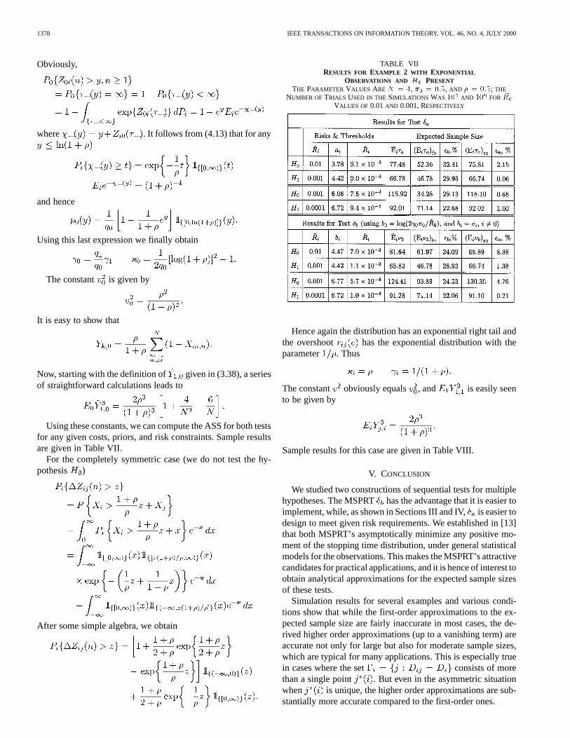
Using these constants, we can compute the ASS for both testsfor any given costs, priors, and risk constraints. Sample resultsare given in Table VII.
For the completely symmetric case (we do not test the hy-pothesis )
After some simple algebra, we obtain
TABLE VIIRESULTS FOR EXAMPLE 2 WITH EXPONENTIAL
OBSERVATIONS AND H PRESENTTHE PARAMETER VALUES AREN = 4, � = 0:5, AND � = 0:5; THE
NUMBER OF TRIALS USED IN THE SIMULATIONS WAS 10 AND 10 FOR �RVALUES OF 0.01AND 0.001, RESPECTIVELY
Hence again the distribution has an exponential right tail andthe overshoot has the exponential distribution with theparameter . Thus
The constant obviously equals , and is easily seento be given by
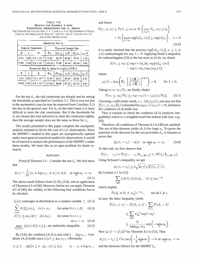
Sample results for this case are given in Table VIII.
V. CONCLUSION
We studied two constructions of sequential tests for multiplehypotheses. The MSPRT has the advantage that it is easier toimplement, while, as shown in Sections III and IV,is easier todesign to meet given risk requirements. We established in [13]that both MSPRT’s asymptotically minimize any positive mo-ment of the stopping time distribution, under general statisticalmodels for the observations. This makes the MSPRT’s attractivecandidates for practical applications, and it is hence of interest toobtain analytical approximations for the expected sample sizesof these tests.
Simulation results for several examples and various condi-tions show that while the first-order approximations to the ex-pected sample size are fairly inaccurate in most cases, the de-rived higher order approximations (up to a vanishing term) areaccurate not only for large but also for moderate sample sizes,which are typical for many applications. This is especially truein cases where the set consists of morethan a single point . But even in the asymmetric situationwhen is unique, the higher order approximations are sub-stantially more accurate compared to the first-order ones.
DRAGALIN et al.: MULTIHYPOTHESIS SEQUENTIAL PROBABILITY RATIO TESTS—PART II 1379
TABLE VIIIRESULTS FOR EXAMPLE 2 WITH
EXPONENTIAL OBSERVATIONS AND H ABSENTTHE PARAMETER VALUES AREN = 4 AND � = 0:3; THE NUMBER OFTRIALS
USED IN THE SIMULATIONS WAS 10 AND 10 FOR �R VALUES OF0:01AND 0:001, RESPECTIVELY
For the test , the risk constraints are sharply met by settingthe thresholds as specified in Corollary 3.1. This is true not justin the asymmetric case (as may be expected from Corollary 3.1)but also in the general case. For, on the other hand, it is moredifficult to meet the risk constraints. But if the thresholds for
are chosen (by trial and error) to meet the constraints tightly,then the average sample sizes are the same as those for.
The results presented in this paper complete the asymptoticanalysis initiated in [4] for the case of i.i.d. observations. Sincethe MSPRT’s studied in this paper are asymptotically optimalunder more general statistical models for observations, it wouldbe of interest to analyze the performance of the MSPRT’s underthese models. We leave this as an open problem for future re-search.
APPENDIX
Proof of Theorem 3.1:Consider the test . We first showthat
as
(A.1)The above result follows from (3.10), (3.8), and an applicationof Theorem 4.5 of [40]. However, before we can apply Theorem4.5 of [40], the validity of the following four conditions has tobe checked:
converges in distribution to a random variable (A.2)
for some (A.3)
for some
as (A.4)
are uniformly integrable (A.5)
By (3.8), the condition (A.2) is true with . Con-dition (A.3) holds since . Obviously,
and hence
(A.6)
It is easily checked that the process , , isa -submartingale for any . Applying Doob’s inequalityfor submartingales [23] to the last term in (A.6), we obtain
where
for
Taking , we finally obtain
(A.7)
Choosing sufficiently small, , one may see thatis bounded by , , and hence
the condition (A.4) holds true.Thus it remains to check the condition (A.5) (uniform inte-
grability) which is a straightforward but tedious task (see, e.g.,[4]).
Therefore, all conditions of Theorem 4.5 in [40] are satisfied.The use of this theorem yields (A.1) for large. To prove theassertion of the theorem for the test procedure, it remains toprove that
as (A.8)
To this end, we first observe that
Using Schwarz’s inequality, we get
By Lemma 2.1 in [13]
which implies
for all
In turn, the latter inequality yields
Now by Theorem 4.1 in [13]. Thus
as
and the theorem follows for the MSPRT.
1380 IEEE TRANSACTIONS ON INFORMATION THEORY, VOL. 46, NO. 4, JULY 2000
For the test the argument is quite similar. In just the sameway as above one can prove that the conditions (A.2)–(A.5) holdfor the process , . Then using (3.3)–(3.12) and [40,Theorem 4.5], we obtain
as
The rest of the argument is essentially the same.
Proof of Theorem 3.2:For the zero–one loss function, theasymptotic equality (3.16) follows from Baum and Veeravalli[4, Theorem 6.1]. To prove this equality for an arbitrary lossfunction we observe first that the risk can be written inthe form
(A.9)
Indeed,
(A.10)
from which (A.9) follows in an obvious manner. Now, since by(3.9)
on
we obtain
Due to the fact that is slowly changing,(see [40, Theorem 4.1]). Furthermore, as
. Hence the value of convergesto which along with the previous equality implies (3.16).
Consider the second test. Obviously, the equality (A.10) istrue for if and are replaced with and , respec-tively. In turn, this equality implies
where
(A.11)
Next, by (3.11)
on
where is the overshoot of the process overthe level at time instant , and hence
Note that by considering the difference of (3.4) and (3.5),of (A.11) can be shown to satisfy
on
which implies the inequalities
Now, as , and by Woodroofe [40,Theorem 4.1], , due to the fact thatis slowly changing. Thus converges to
. This fact together with the previous inequalities yields (3.17)and the theorem follows.
Proof of Theorem 3.3:Consider the test procedure. Ar-guments identical to those used in the proof of Theorem 3.1 maybe used to establish that it is sufficient to prove (3.32) only for.
Now recall from (3.29) that
(A.12)
where is a random walk withincrements having positive mean ,
, and
(A.13)It is desirable to replace the maximization over in
(A.13) by a maximization over only thosecorresponding tothe nearest hypotheses. To this end, let
where is as defined in (3.25).Due to assumption (3.23), we have
for some
for some
DRAGALIN et al.: MULTIHYPOTHESIS SEQUENTIAL PROBABILITY RATIO TESTS—PART II 1381
where
Since is a random walk with mean zero and finitesecond moment, , by the Baum–Katz rate ofconvergence in the law of large numbers [3]2
for all
which along with the above inequality yields
Hence, for we can write of (A.13) as
(A.14)
with
(A.15)
where is defined in (3.28). The proof of (3.32) for runsalmost parallel to that of Dragalin [11, Lemma 1 ] and is basedon Zhang [41, Theorem 3]. In order to apply this theorem, thefollowing conditions need to be checked:
as for some
(A.16)
as (A.17)
for some (A.18)
is uniformly integrable (A.19)
for any
(A.20)
converges in distribution to an integrable
random variable (A.21)
Then, by Zhang [41, Theorem 3]
as (A.22)
where
(A.23)
To prove (A.16) we rewrite in the following form:
2See also Chow and Lai [8] for a one-sided versions that may be applied inthe case considered.
where with
which is a zero-mean random walk. Letand
(In what follows we omit the indexin , , , etc., forbrevity.) Then
(A.24)
By the submartingale inequality, the first probability in (A.24)can be estimated above
Since , we have thatas . Then, by the uniform integrability of
and hence
Using the same arguments, it may be shown that the secondprobability in (A.24)
The proof of (A.16) is complete.Let . The proof of (A.17) is a direct appli-
cation of a submartingale inequality and uniform integrabilityof
Similar to the proof of (A.4) we have that
1382 IEEE TRANSACTIONS ON INFORMATION THEORY, VOL. 46, NO. 4, JULY 2000
as . Now, the uniform integrability of yields
which proves (A.17).Verification of (A.18) is similar to, but simpler than, that pre-
sented in the proof of (A.17) and is omitted.Conditions (3.6) and (3.7) (slowly changing) and conditions
(A.19)–(A.21) are used in [41, proof of Theorem 3] to obtain theuniform integrability of the overshootand to prove that as . The former followsfrom [10, Lemma 4.2] which states that is bounded above bya uniformly integrable random variable. The latter convergenceis proved in the next paragraph.
Using Theorem 20.1 of Bhattacharya and Rao [5] withand , we have (under the
assumption of our theorem)
(A.25)
where . On the other hand,transformation of variables and first-order Taylor expansion for
in the first integral yield (as )
(A.26)
By denote the second integral in (A.25). Obviously we havethe following estimates for :
which show that
as (A.27)
The relations (A.14) and (A.25)–(A.27) give
as
Substituting the above limiting value for in (A.22), the re-quired asymptotic result (3.32) follows.
Now, consider the MSPRT . It follows from [13, eq. (2.2)]that if , , then
Thus may be obtained to within a constant factor,, by replacing with in (3.32).
REFERENCES
[1] P. Armitage, “Sequential analysis with more than two alternativehypotheses, and its relation to discriminant function analysis,”J. Roy.Statist. Soc. B., vol. 12, pp. 137–144, 1950.
[2] P. A. Bakut, I. A. Bolshakov, B. M. Gerasimov, A. A. Kuriksha, V. G.Repin, G. P. Tartakovsky, and V. V. Shirokov,Statistical Radar Theory,G. P. Tartakovsky, Ed. Moscow, USSR: Sov. Radio, 1963, vol. 1. InRussian.
[3] L. E. Baum and M. Katz, “Convergence rates in the law of large num-bers,”Trans. Amer. Math. Soc., vol. 120, pp. 108–123, 1965.
[4] C. W. Baum and V. V. Veeravalli, “A sequential procedure for multihy-pothesis testing,”IEEE Trans. Inform. Theory, vol. 40, pp. 1994–2007,Nov. 1994.
[5] R. N. Bhattacharya and R. R. Rao,Normal Approximations and Asymp-totic Expansions. New York: Wiley, 1986.
[6] J. J. Bussgang, “Sequential methods in radar detection,”Proc. IEEE, vol.58, pp. 731–743, 1970.
[7] H. Chernoff, “Sequential design of experiments,”Ann. Math. Statist.,vol. 30, pp. 755–770, 1959.
[8] Y. S. Chow and T. L. Lai, “Some one-sided theorems on the tail distribu-tion of sample sums with applications to the last time and largest excessof boundary crossing,”Trans. Amer. Math. Soc., vol. 208, pp. 51–72,1975.
[9] V. P. Dragalin, “Asymptotic solution of a problem of detecting a signalfrom k channels,”Russian Math. Surveys, vol. 42, no. 3, pp. 213–214,1987.
[10] , “Asymptotic solution of a problem of signal searching in multi-channel system,”Math. Res., Acad. Sci. Moldova, vol. 109, pp. 15–35,1989. In Russian.
[11] , “Asymptotics for a sequential selection procedure,”Statistics andDecisions, pp. 123–137, 1999. Suppl. Issue no. 4.
[12] V. P. Dragalin and A. A. Novikov, “Adaptive sequential tests for com-posite hypotheses,” Inst. Appl. Math. Informatics, Milan, Italy, Tech.Rep. 94, 1994.
[13] V. P. Dragalin, A. G. Tartakovsky, and V. Veeravalli, “Multihypothesissequential probability ratio tests—Part I: Asymptotic optimality,”IEEETrans. Inform. Theory, vol. 45, pp. 2448–2461, Nov. 1999.
[14] B. Emlsee, S. K. Rogers, M. P. DeSimio, and R. A. Raines, “Completeautomatic target recognition system for tactical forward-looking infraredimages,”Opt. Eng., vol. 36, pp. 2593–2603, Sept. 1997.
[15] T. S. Ferguson,Mathematical Statistics: A Decision Theoretic Ap-proach. New York, NY, London, U.K.: Academic, 1967.
[16] M. M. Fishman, “Average duration of asymptotically optimal multi-alternative sequential procedure for recognition of processes,”Sov. J.Commun.. Technol. Electron., vol. 30, pp. 2541–2548, 1987.
[17] K. S. Fu, Sequential Methods in Pattern Recognition andLearning. New York: Academic, 1968.
[18] G. K. Golubev and R. Z. Khas’minskii, “Sequential testing for sev-eral signals in Gaussian white noise,”Theory Prob. Appl., vol. 28, pp.573–584, 1983.
[19] C. Jennison and B. W. Turnbull,Group Sequential Methods with Appli-cations to Clinical Trials. New York, NY; London, U.K.: Chapman &Hall/CRC, 2000.
[20] J. Kiefer and J. Sacks, “Asymptotically optimal sequential inference anddesign,”Ann. Math. Statist., vol. 34, pp. 705–750, 1963.
[21] T. L. Lai and D. Siegmund, “A nonlinear renewal theory with applica-tions to sequential analysis, I,”Ann. Statist., vol. 5, pp. 946–954, 1977.
[22] , “A nonlinear renewal theory with applications to sequential anal-ysis, II,” Ann. Statist., vol. 7, pp. 60–76, 1979.
[23] R. S. Liptser and A. N. Shiryaev,Theory of Martingales. Dordrecht,The Netherlands: Kluwer, 1989.
[24] M. Long, Airborne Early Warning System Concepts. Boston, MA,London, U.K.: Artech, 1992.
[25] G. Lorden, “Nearly-optimal sequential tests for finitely many parametervalues,”Ann. Statist., vol. 5, pp. 1–21, 1977.
DRAGALIN et al.: MULTIHYPOTHESIS SEQUENTIAL PROBABILITY RATIO TESTS—PART II 1383
[26] M. B. Marcus and P. Swerling, “Sequential detection in radar with mul-tiple resolution elements,”IRE Trans. Inform. Theory, vol. IT-8, pp.237–245, Apr. 1962.
[27] S. C. Port, “Escape probability for a half-line,”Ann. Math. Statist., vol.35, pp. 1351–1355, 1964.
[28] D. Siegmund, Sequential Analysis: Tests and Confidence Inter-vals. New York: Springer-Verlag, 1985.
[29] Yu. G. Sosulin and M. M. Fishman,Theory of Sequential Decisions andIts Applications. Moscow, USSR: Radio i Svyaz, 1985. In Russian.
[30] A. G. Tartakovsky, S. Kligys, and A. Petrov, “Adaptive sequential algo-rithms for detecting targets in heavy IR clutter,” inSPIE Proc.: Signaland Data Processing of Small Targets, vol. 3809, O. E. Drummond, Ed.,Denver, CO, July 18–23, 1999, pp. 119–130.
[31] A. G. Tartakovskii, “Sequential testing of many simple hypotheses withdependent observations,”Probl. Inform. Transm., vol. 24, pp. 299–309,1988.
[32] A. G. Tartakovsky,Sequential Methods in the Theory of InformationSystems. Moscow, Russia: Radio i Svyaz, 1991. In Russian.
[33] , “Asymptotically optimal sequential tests for nonhomogeneousprocesses,”Sequential Anal., vol. 17, no. 1, pp. 33–61, 1998.
[34] , “Asymptotic optimality of certain multi-alternative sequentialtests: Non-i.i.d. case,”Statist. Infer. Stochastic Processes, vol. 1, no. 3,pp. 265–295, 1998.
[35] A. G. Tartakovsky and I. A. Ivanova, “Approximations in sequentialrules for testing composite hypotheses and their accuracy in the problemof signal detection from post-detector data,”Probl. Inform. Transm., vol.28, pp. 63–74, 1992.
[36] V. V. Veeravalli and C. W. Baum, “Asymptotic efficiency of a sequen-tial multihypothesis test,”IEEE Trans. Inform. Theory, vol. 41, pp.1994–1997, Nov. 1995.
[37] , “Hybrid acquisition of direct sequence CDMA signals,”Int. J.Wireless Inform. Networks, vol. 3, pp. 55–65, Jan. 1996.
[38] N. V. Verdenskaya and A. G. Tartakovskii, “Asymptotically optimal se-quential testing of multiple hypotheses for nonhomogeneous Gaussianprocesses in an asymmetric situation,”Theory Prob. Appl., vol. 36, pp.536–547, 1991.
[39] J. Whitehead,The Design and Analysis of Sequential Clinical Trials,2nd ed. Chichester, U.K.: Wiley, 1997. Revised.
[40] M. Woodroofe, Nonlinear Renewal Theory in Sequential Anal-ysis. Philadelphia, PA: SIAM, 1982.
[41] C. H. Zhang, “A nonlinear renewal theory,”Ann. Probab., vol. 16, pp.793–825, 1988.