arXiv: arXiv:1602.07933

BOOTSTRAP INFERENCE WHEN USING MULTIPLE IMPUTATION

By Michael Schomaker and Christian Heumann

University of Cape Town∗ and Ludwig-Maximilians Universitat Munchen†

Many modern estimators require bootstrapping to calculate con-fidence intervals because either no analytic standard error is availableor the distribution of the parameter of interest is non-symmetric.It remains however unclear how to obtain valid bootstrap inferencewhen dealing with multiple imputation to address missing data. Wepresent four methods which are intuitively appealing, easy to imple-ment, and combine bootstrap estimation with multiple imputation.We show that three of the four approaches yield valid inference, butthat the performance of the methods varies with respect to the num-ber of imputed data sets and the extent of missingness. Simulationstudies reveal the behavior of our approaches in finite samples. Atopical analysis from HIV treatment research, which determines theoptimal timing of antiretroviral treatment initiation in young chil-dren, demonstrates the practical implications of the four methods ina sophisticated and realistic setting. This analysis suffers from miss-ing data and uses the g-formula for inference, a method for which nostandard errors are available.

The published version of this working paper can be cited as follows:

Schomaker, M., Heumann, C.Bootstrap Inference When Using Multiple ImputationStatistics in Medicine, 37(14):2252-2266http://dx.doi.org/10.1002/sim.7654

1. Introduction. Multiple imputation (MI) is a popular method to address missing data.Based on assumptions about the data distribution (and the mechanism which gives rise to themissing data) missing values can be imputed by means of draws from the posterior predictivedistribution of the unobserved data given the observed data. This procedure is repeated tocreate M imputed data sets, the analysis is then conducted on each of these data sets and theM results (M point and M variance estimates) are combined by a set of simple rules [1].

During the last 30 years a lot of progress has been made to make MI useable for differentsettings: implementations are available in several software packages [2, 3, 4, 5], review articlesprovide guidance to deal with practical challenges [6, 7, 8], non-normal –possibly categorical–variables can often successfully be imputed [9, 3, 6], useful diagnostic tools have been suggested[3, 10], and first attempts to address longitudinal data and other complicated data structureshave been made [11, 4].

While both opportunities and challenges of multiple imputation are discussed in the litera-ture, we believe an important consideration regarding the inference after imputation has beenneglected so far: if there is no analytic or no ideal solution to obtain standard errors for the

Keywords and phrases: missing data, resampling, data augmentation, g-methods, causal inference, HIV

1

arX

iv:1

602.

0793

3v6

[st

at.M

E]

5 J

un 2

018

2

parameters of the analysis model, and nonparametric bootstrap estimation is used to estimatethem, it is unclear how to obtain valid inference – in particular how to obtain appropriateconfidence intervals. Moreover, bootstrap estimation is also often used when a parameter’sdistribution is assumed to be non-normal and bootstrap inference with missing data is thennot clear either. As we will explain below, many modern statistical concepts, often applied toinform policy guidelines or enhance practical developments, rely on bootstrap estimation. It istherefore necessary to have guidance for bootstrap estimation for multiply imputed data.

In general, one can distinguish between two approaches for bootstrap inference when usingmultiple imputation: with the first approach, M imputed datsets are created and bootstrapestimation is applied to each of them; or, alternatively, B bootstrap samples of the original dataset (including missing values) are drawn and in each of these samples the data are multiplyimputed. For the former approach one could use bootstrapping to estimate the standard errorin each imputed data set and apply the standard MI combining rules; alternatively, the B×Mestimates could be pooled and 95% confidence intervals could be calculated based on the 2.5th

and 97.5th percentiles of the respective empirical distribution. For the latter approach eithermultiple imputation combining rules can be applied to the imputed data of each bootstrapsample to obtain B point estimates which in turn may be used to construct confidence intervals;or the B ×M estimates of the pooled data are used for interval estimation.

To the best of our knowledge, the consequences of using the above approaches have notbeen studied in the literature before. The use of the bootstrap in the context of missing datahas often been viewed as a frequentist alternative to multiple imputation [12], or an option toobtain confidence intervals after single imputation [13]. The bootstrap can also be used to createmultiple imputations [14]. However, none of these studies have addressed the construction ofbootstrap confidence intervals when data needs to be multiply imputed because of missing data.As emphasized above, this is however of particularly great importance when standard errorsof the analysis model cannot be calculated easily, for example for causal inference estimators(e.g. the g-formula).

It is not surprising that the bootstrap has nevertheless been combined with multiple impu-tation for particular analyses. Multiple imputation of bootstrap samples has been implementedin [15, 16, 17, 18], whereas bootstrapping the imputed data sets was preferred by [19, 20, 21].Other work doesn’t offer all details of the implementation [22]. All these analyses give howeverlittle justification for the chosen method and for some analyses important details on how theconfidence intervals were calculated are missing; it seems that pragmatic reasons as well ascomputational efficiency typically guide the choice of the approach. None of the studies offera statistical discussion of the chosen method.

The present article demonstrates the implications of different methods which combine boot-strap inference with multiple imputation. It is novel in that it introduces four different, intu-itively appealing, bootstrap confidence intervals for data which require multiple imputation,illustrates their intrinsic features, and argues which of them is to be preferred.

Section 2 introduces our motivating analysis of causal inference in HIV research. The differ-ent methodological approaches are described in detail in Section 3 and are evaluated by meansof both numerical investigations (Section 4) and theoretical considerations (Section 6). Theimplications of the different approaches are further emphasized in the data analysis of Section5. We conclude in Section 7.

BOOTSTRAP INFERENCE WHEN USING MULTIPLE IMPUTATION 3

2. Motivation. During the last decade the World Health Organization (WHO) updatedtheir recommendations on the use of antiretroviral drugs for treating and preventing HIV in-fection several times. In the past, antiretroviral treatment (ART) was only given to a childif his/her measurements of CD4 lymphocytes fell below a critical value or if a clinically se-vere event (such as tuberculosis or persistent diarrhoea) occurred. Based on both increasedknowledge from trials and causal modeling studies, as well as pragmatic and programmaticconsiderations, these criteria have been gradually expanded to allow earlier treatment initia-tion in children: in 2013 it was suggested that all children who present under the age of 5 aretreated immediately, while for older children CD4-based criteria still existed. By the end of2015 WHO decided to recommend immediate treatment initiation in all children and adults.ART has shown to be effective and to reduce mortality in infants and adults [23, 24, 25], butconcerns remain due to a potentially increased risk of toxicities, early development of drugresistance, and limited future options for people who fail treatment.

It remains therefore important to investigate the effect of different treatment initiation ruleson mortality, morbidity and child development outcomes; however given the shift in ARTguidelines towards earlier treatment initiation it is not ethically possible anymore to conduct atrial which answers this question in detail. Thus, observational data can be used to obtain therelevant estimates. Methods such as inverse probability weighting of marginal structural mod-els, the g-computation formula, and targeted maximum likelihood estimation can be used toobtain estimates in complicated longitudinal settings where time-varying confounders affectedby prior treatment are present — such as, for example, CD4 count which influences both theprobability of ART initiation and outcome measures [26, 27].

In situations where treatment rules are dynamic, i.e. where they are based on a time-varyingvariable such as CD4 lymphocyte count, the g-computation formula [28] is the intuitive methodto use. It is computationally intensive and allows the comparison of outcomes for differenttreatment options; confidence intervals are typically based on non-parametric bootstrap esti-mation. However, in resource limited settings data may be missing for administrative, logistic,and clerical reasons, as well as due to loss to follow-up and missed clinic visits. Dependingon the underlying assumptions about the reasons for missing data, this problem can eitherbe addressed by the g-formula directly or by using multiple imputation. However, it is notimmediately clear how to combine multiple imputation with bootstrap estimation too obtainvalid confidence intervals.

3. Methodological Framework. Let D be a n × (p + 1) data matrix consisting of anoutcome variable y = (y1, . . . , yn)′ and covariates Xj = (X1j , . . . , Xnj)

′, j = 1, . . . , p. The1 × p vector xi = (xi1, . . . , xip) contains the ith observation of each of the p covariates andX = (x1

′, . . . ,xn′)′ is the matrix of all covariates. Suppose we are interested in estimating

θ = (θ1, . . . , θk)′, k ≥ 1, which may be a regression coefficient, an odds ratio, a factor loading,

or an counterfactual outcome. If some data are missing, making the data matrix to consistof both observed and missing values, D = {Dobs,Dmis}, and the missingness mechanism isignorable, valid inference for θ can be obtained using multiple imputation. Following Rubin [1]we regard valid inference to mean that the point estimate θ for θ is approximately unbiasedand that interval estimates are randomization valid in the sense that actual interval coverageequals the nominal interval coverage.

Under multiple imputation M augmented sets of data are generated, and the imputations(which replace the missing values) are based on draws from the posterior predictive distribution

4

of the missing data given the observed data p(Dmis|Dobs) =∫p(Dmis|Dobs;ϑ) p(ϑ|Dobs) dϑ, or

an approximation thereof. The point estimate for θ is

ˆθMI =1

M

M∑m=1

θm(3.1)

where θm refers to the estimate of θ in the mth imputed set of data D(m), m = 1, . . . ,M .Variance estimates can be obtained using the between imputation covariance V = (M −1)−1

∑m(θm − ˆθMI)(θm − ˆθMI)

′and the average within imputation covariance W = M−1∑

m Cov(θm):

Cov(ˆθMI) = W +M + 1

MV =

1

M

M∑m=1

Cov(θm)(3.2)

+M + 1

M(M − 1)

M∑m=1

(θm − ˆθMI)(θm − ˆθMI)′.

For the scalar case this equates to

Var(ˆθMI) =1

M

M∑m=1

Var(θm) +M + 1

M(M − 1)

M∑m=1

(θm − ˆθMI)2 .

To construct confidence intervals for ˆθMI in the scalar case, it may be assumed that Var(ˆθMI)− 1

2 (ˆθMI−θ) follows a tR-distribution with approximately R = (M − 1)[1 + {MW/(M + 1)V }]2 degreesof freedom [29], though there are alternative approximations, especially for small samples [30].Note that for reliable variance estimation M should not be too small; see White et al. [6] forsome rules of thumb.

Consider the situation where there is no analytic or no ideal solution to estimate Cov(θm),for example when estimating the treatment effect in the presence of time-varying confoundersaffected by prior treatment using g-methods [31, 26]. If there are no missing data, bootstrappercentile confidence intervals may offer a solution: based on B bootstrap samples D∗b , b =

1, . . . , B, we obtain B point estimates θ∗b . Consider the ordered set of estimates Θ∗B = {θ∗(b); b =

1, . . . , B}, where θ∗(1) < θ∗(2) < . . . < θ∗(B); the bootstrap 1 − 2α% confidence interval for θ isthen defined as

[θlower; θupper] = [θ∗,α; θ∗,1−α]

where θ∗,α denotes the α-percentile of the ordered bootstrap estimates Θ∗B. However, in the

presence of missing data the construction of confidence intervals is not immediately clear as θcorresponds to M estimates θ1, . . . , θM , i.e. θm is the point estimate calculated from the mth

imputed data set. It seems intuitive to consider the following four approaches:

• Method 1, MI Boot (pooled sample [PS]): Multiple imputation is utilized for thedata set D = {Dobs,Dmis}. For each of the M imputed data sets Dm, B bootstrap samplesare drawn which yields M × B data sets D∗m,b; b = 1, . . . , B;m = 1, . . . ,M . In each of

these data sets the quantity of interest is estimated, that is θ∗m,b. The pooled sample of

BOOTSTRAP INFERENCE WHEN USING MULTIPLE IMPUTATION 5

ordered estimates Θ∗MIBP = {θ∗(m,b); b = 1, . . . , B;m = 1, . . . ,M} is used to construct the

1− 2α% confidence interval for θ:

[θlower; θupper]MIBP = [θ∗,αMIBPθ∗,1−αMIBP ](3.3)

where θ∗,αMIBP is the α-percentile of the ordered bootstrap estimates Θ∗MIBP.

• Method 2, MI Boot: Multiple imputation is utilized for the data set D = {Dobs,Dmis}.For each of the M imputed data sets Dm, B bootstrap samples are drawn which yieldsM × B data sets D∗m,b; b = 1, . . . , B; m = 1, . . . ,M . The bootstrap samples are used

to estimate the standard error of (each scalar component of) θm in each imputed data

set respectively, i.e. Var(θm) = (B − 1)−1∑

b(θm,b −ˆθm)2 with ˆθm = B−1

∑b θm,b. This

results in M point estimates (calculated from the imputed, but not yet bootstrappeddata), and M standard errors (calculated from the respective bootstrap samples). Moregenerally, Cov(θm) can be estimated in each imputed data set using bootstrapping, thusallowing the use of (3.2) and standard multiple imputation confidence interval construc-tion, possibly based on a tR-distribution.

• Method 3, Boot MI (pooled sample [PS]): B bootstrap samples D∗b (includingmissing data) are drawn and multiple imputation is utilized in each bootstrap sample.Therefore, there are B × M imputed data sets D∗b,1, . . . ,D∗b,M which can be used to

obtain the corresponding point estimates θ∗b,m. The set of the pooled ordered estimates

Θ∗BMIP = {θ∗(b,m); b = 1, . . . , B;m = 1, . . . ,M} can then be used to construct the 1−2α%confidence interval for θ:

[θlower; θupper]BMIP = [θ∗,αBMIP; θ∗,1−αBMIP ](3.4)

where θ∗,αBMIP is the α-percentile of the ordered bootstrap estimates Θ∗BMIP.

• Method 4, Boot MI: B bootstrap samples D∗b (including missing data) are drawn, andeach of them is imputed M times. Therefore, there are M imputed data sets, D∗b,1, . . . ,D∗b,M , which are associated with each bootstrap sample D∗b . They can be used to ob-

tain the corresponding point estimates θ∗b,m. Thus, applying (3.1) to the estimates of

each bootstrap sample yields B point estimates ˆθ∗b = M−1∑

m θ∗b,m for θ. The set of

ordered estimates Θ∗BMI = {θ∗(b); b = 1, . . . , B} can then be used to construct the 1−2α%confidence interval for θ:

[θlower; θupper]BMI = [θ∗,αBMI; θ∗,1−αBMI ](3.5)

where θ∗,αBMI is the α-percentile of the ordered bootstrap estimates Θ∗BMI.

While all of the methods described above are straightforward to implement it is unclear ifthey yield valid inference, i.e. if the actual interval coverage level equals the nominal coveragelevel. Before we delve into some theoretical and practical considerations we expose some of theintrinsic features of the different interval estimates using Monte Carlo simulations.

6

4. Simulation Studies. To study the performance of the methods introduced above weconsider four simulation settings: a simple one, to ensure that these comparisons are not compli-cated by the simulation setup; a more complicated one, to study the four methods under a moresophisticated variable dependence structure; a survival analysis setting to allow comparisonsbeyond a linear regression setup; and a complex longitudinal setting where time-dependentconfounding (affected by prior treatment) is present, to allow comparisons to our data analysisin Section 5.

Setting 1: We simulate a normally distributed variable X1 with mean 0 and variance 1. Wethen define µy = 0 + 0.4X1 and θ = βtrue = (0, 0.4)′. The outcome is generated from N(µy, 2)and the analysis model of interest is the linear model. Values of X1 are defined to be missingwith probability

πX1(y) = 1− 1

(0.25y)2 + 1.

With this, about 16% of values of X1 were missing (at random).

Setting 2: The observations for 6 variables are generated using the following normal and bino-mial distributions: X1 ∼ N(0, 1), X2 ∼ N(0, 1), X3 ∼ N(0, 1), X4 ∼ B(0.5), X5 ∼ B(0.7), andX6 ∼ B(0.3). To model the dependency between the covariates we use a Clayton Copula [32]with a copula parameter of 1 which indicates moderate correlations among the covariates. Wethen define µy = 3 − 2X1 + 3X3 − 4X5 and θ = βtrue = (3,−2, 0, 3, 0,−4, 0)′. The outcome isgenerated from N(µy, 2) and the analysis model of interest is the linear model. Values of X1

and X3 are defined to be missing (at random) with probabilities

πX1(y) = 1− 1

(ay)2 + 1, πX3(X4) = 1− 1

bX34 + 1.05

.

where a and b equate to 0.75 and 0.25 in a low missingness setting (and to 0.4 and 2.5 in ahigh missingness setting). This yields about 6% and 14% (45% and 38%) of missing values forX1 and X3 respectively.

Setting 3: This setting is inspired by the analysis and data in Schomaker et al. [33]. We simulateX1 ∼ logN(4.286, 1.086) and X2 ∼ logN(10.76, 1.8086). Again, the dependency of the variablesis modeled with a Clayton copula with a copula parameter of 1. Survival times y are simulatedfrom − log(U)/h0{exp(Xβ)} where U is drawn from a distribution that is uniform on theinterval [0, 1], h0 = 0.1, and the linear predictor Xβ is defined as −0.3 lnX1 + 0.3 log10X2.Therefore, βtrue = (−0.3, 0.3)′. Censoring times are simulated as − log(U)/0.2. The observedsurvival time T is thus min(y, C). Values of X1 are defined to be missing based on the followingfunction:

πX1(T ) = 1− 1

(0.075T )2 + 1.

This yields about 8% of missing values.

Setting 4: This setting is inspired by our data analysis from Section 5. We generate longitudinaldata (t = 0, 1, . . . , 12) for 3 time-dependent confounders (Lt = {L1

t , L2t , L

3t }), an outcome (Yt),

BOOTSTRAP INFERENCE WHEN USING MULTIPLE IMPUTATION 7

an intervention (At), as well as baseline data for 7 variables, using structural equation models[34]. The data generating mechanism and the motivation thereof is described in Appendix B.In this simulation we are interested in an counterfactual outcome Yt which would have beenobserved under 2 different intervention rules dj , j = 1, 2, which assign treatment (At) alwaysor never. We denote these target quantities as ψ1 and ψ2 and their true values are −1.03and −2.45 respectively. They can be estimated using the sequential g-formula, with bootstrapconfidence intervals, see Appendix A for more details.

Values of L1t , L

2t , L

3t , Yt are set to be missing based on a MAR process as described in

Appendix B. This yields about 10%, 31%, 22% and 44% of missing baseline values, and 10%,1%, 1%, and 2% of missing follow-up values.

In all 4 settings multiple imputation is utilized with Amelia II under a joint modelingapproach, see Honaker et al. [3] and Section 6 for details. In settings 1-3 the probability of amissing observation depends on the outcome. One would therefore expect parameter estimatesin a regression model of a complete case analysis to be biased, but estimates following multipleimputation to be approximately unbiased [35, 36].

We estimate the confidence intervals for the parameters of interest using the aforementionedfour approaches, as well as using the analytic standard errors obtained from the linear modeland the Cox proportional hazards model (method “no bootstrap”) for the first three settings.The “no bootstrap” method serves therefore as a gold standard and reference for the othermethods. We generate n = 1000 observations, B = 200 bootstrap samples, and M = 10 impu-tations. Based on R = 1000 simulation runs we evaluate the coverage probability and medianwidth of the respective confidence intervals.

Results: The computation time for Boot MI was always greater than for MI Boot, for exampleby a factor of 13 in the first simulation setting and by a factor of 1.3 in the fourth setting.

In all settings the point estimates for β were approximately unbiased.Table 1 summarizes the main results of the simulations. Using no bootstrapping yields

estimated coverage probabilities of about 95%, for all parameters and settings, as one wouldexpect.

Bootstrapping the imputed data (MI Boot, MI Boot [PS]) yields estimated coverage proba-bilities of about 95% and confidence interval widths which are similar to each other, except forthe high missingness setting of simulation 2. The standard errors for each component of β assimulated in the 1000 simulation runs were almost identical to the mean estimated standarderrors under MI Boot, which suggests good standard error estimation of the latter approach.In the first simulation setting the coverage of MI Boot pooled is a bit too low for M = 10(93%), but is closer to 95% if M is large (M = 20, Figure 1).

Imputing the bootstrapped data (Boot MI, Boot MI [PS]) led to overall good results withcoverage probabilities close to the nominal level, except for the high missingness setting of sim-ulation 2; however, using the pooled samples led to somewhat higher coverage probabilities andthe interval widths were slightly different from the estimates obtained under no bootstrapping.

Figure 1 shows the coverage probability of the interval estimates for β1 in the first simulationsetting given the number of imputations.

As predicted by MI theory, using multiple imputation needs generally a reasonable amountof imputed data sets to perform well – no matter whether bootstrapping is used for standard

8

Table 1Results of the simulation studies: estimated coverage probability (top), median confidence intervals width

(middle), and standard errors for different methods (bottom). The bottom panel lists standard errors estimatedfrom the 1000 point estimates of the simulation (“simulated”) and the mean estimated standard error across

the simulated data sets, for both the analytical standard error (“no bootstrap”) and the bootstrap standard error(“MI Boot”). All results are based on 200 bootstrap samples and 10 imputations.

Method Setting 1 Setting 2 (low missingness) Setting 3

β1 β1 β2 β3 β4 β5 β6 β1 β2

Cov

erage

Pro

babilit

y 1) MI Boot (PS) 93% 95% 95% 94% 94% 95% 95% 95% 95%2) MI Boot 95% 95% 95% 95% 94% 95% 95% 95% 95%3) Boot MI (PS) 97% 96% 95% 96% 95% 96% 96% 96% 96%4) Boot MI 94% 94% 94% 94% 94% 94% 94% 94% 94%5) no bootstrap 95% 95% 95% 95% 95% 95% 96% 95% 95%

Med

ian

CI

Wid

th

1) MI Boot (PS) 0.30 0.33 0.33 0.33 0.60 0.68 0.62 0.25 0.312) MI Boot 0.31 0.34 0.34 0.34 0.61 0.69 0.63 0.26 0.313) Boot MI (PS) 0.35 0.36 0.35 0.35 0.64 0.72 0.66 0.26 0.314) Boot MI 0.30 0.33 0.33 0.33 0.60 0.67 0.62 0.24 0.305) no bootstrap 0.31 0.34 0.34 0.34 0.61 0.69 0.63 0.25 0.31

Std

.

Err

or simulated 0.08 0.09 0.09 0.09 0.16 0.18 0.16 0.06 0.08

no bootstrap 0.08 0.09 0.09 0.09 0.16 0.18 0.16 0.06 0.08MI Boot 0.08 0.09 0.09 0.09 0.16 0.18 0.16 0.07 0.08

Method Setting 2 (high missingness) Setting 4

β1 β2 β3 β4 β5 β6 ψ1 ψ2

Cov

erage

Pro

babilit

y 1) MI Boot (PS) 89% 91% 92% 91% 92% 92% 94% 94%2) MI Boot 91% 93% 94% 94% 94% 94% 94% 94%3) Boot MI (PS) 96% 97% 98% 98% 97% 98% 94% 94%4) Boot MI 90% 93% 93% 95% 94% 94% 94% 92%5) no bootstrap 91% 93% 94% 94% 94% 94% – –

Med

ian

CI

Wid

th

1) MI Boot (PS) 0.44 0.40 0.44 0.79 0.87 0.78 0.20 0.212) MI Boot 0.48 0.44 0.49 0.87 0.95 0.86 0.20 0.223) Boot MI (PS) 0.58 0.51 0.59 1.03 1.12 1.01 0.21 0.234) Boot MI 0.47 0.43 0.47 0.84 0.92 0.82 0.20 0.225) no bootstrap 0.48 0.44 0.49 0.87 0.95 0.86 – –

Std

.

Err

or simulated 0.12 0.11 0.12 0.22 0.24 0.21 – –

no bootstrap 0.12 0.12 0.12 0.22 0.24 0.22 – –MI Boot 0.12 0.11 0.12 0.22 0.24 0.21 – –

error estimation or not (MI Boot, no bootstrap). Boot MI may perform well even for M < 5,but the pooled approach has a tendency towards coverage probabilities > 95%. For M = 1 theestimated coverage probability of Boot MI is too large in the above setting.

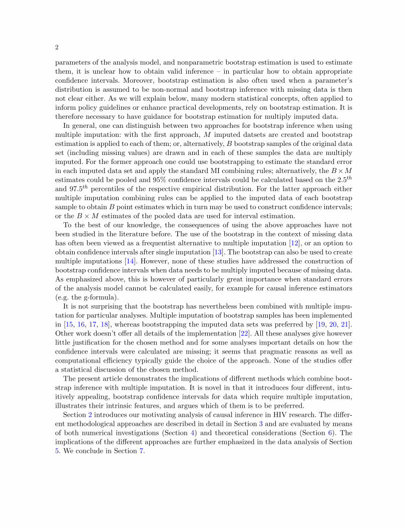
Figure 2 offers more insight into the behaviour of ‘Boot MI (PS)’ and ‘MI Boot (PS)’ byvisualizing both the bootstrap distributions in each imputed data set (method MI Boot [PS])as well as the distribution of the estimators in each bootstrap sample (method Boot MI [PS]):one can see the slightly wider spectrum of values in the distributions related to ‘Boot MI (PS)’explaining the somewhat larger confidence interval in the first simulation setting.

More explanations and interpretations of the above results are given in Section 6.

5. Data Analysis. Consider the motivating question introduced in Section 2. We areinterested in comparing mortality with respect to different antiretroviral treatment strategiesin children between 1 and 5 years of age living with HIV. We use data from two big HIV

BOOTSTRAP INFERENCE WHEN USING MULTIPLE IMPUTATION 9

0.80

0.85

0.90

0.95

1.00

1 2 3 4 5 10 20Number of Imputations

Cov

erag

e P

roba

bilit

y

MethodBoot MI

Boot MI (PS)

MI Boot

MI Boot (PS)

no bootstrap

original data

Fig 1: Coverage probability of the interval estimates for β1 in the first simulation settingdependent on the number of imputations. Results related to the complete simulated data, i.e.before missing data are generated, are labelled “original data”.

treatment cohort collaborations (IeDEA-SA, [37]; IeDEA-WA, [38]) and evaluate mortality for3 years of follow-up. Our analysis builds on a recently published analysis by Schomaker et al.[17].

For this analysis, we are particularly interested in the cumulative mortality difference be-tween strategies (i) ‘immediate ART initiation’ and (ii) ‘assign ART if CD4 count < 350cells/mm3 or CD4% < 15%’, i.e. we are comparing current practices with those in place in2006. We can estimate these quantities using the g-formula, see Appendix A for a compre-hensive summary of our implementation details and assumptions. The standard way to obtain95% confidence intervals for this method is using bootstrapping. However, baseline data ofCD4 count, CD4%, HAZ, and WAZ are missing: 18%, 28%, 40%, and 25% respectively. Weuse multiple imputation (using Amelia II [3]) to impute this data. We also impute follow-updata after nine months without any visit data, as from there on it is plausible that follow-upmeasurements that determine ART assignment (e.g. CD4 count) were taken (and are thusneeded to adjust for time-dependent confounding) but were not electronically recorded, proba-bly because of clerical and administrative errors. Under different assumptions imputation maynot be needed. To combine the M = 10 imputed data sets with bootstrap estimation (B = 200)we use the four approaches introduced in Section 3: MI Boot, MI Boot (PS), Boot MI, andBoot MI (PS).

Three year mortality for immediate ART initiation was estimated as 6.08%, whereas mortal-

10

0.0 0.2 0.4 0.6

02

46

MI Boot (PS)

Den

sity

0.0 0.2 0.4 0.6

05

1020

Boot MI (PS)

Den

sity

Fig 2: Estimate of β1 in the first simulation setting, for a random simulation run: distributionof ‘MI Boot (pooled)’ for each imputed dataset (top) and distribution of ‘Boot MI (PS)’ for 50random bootstrap samples (PS). Point estimates are marked by the black tick marks on thex-axis.

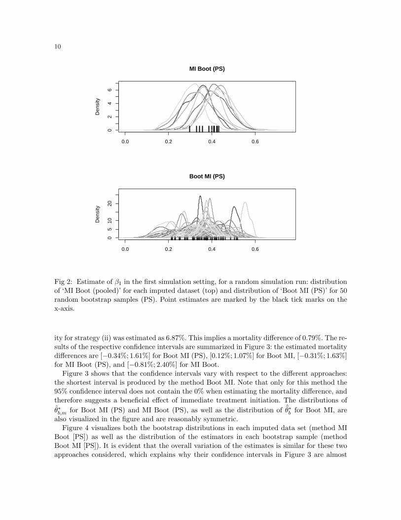
ity for strategy (ii) was estimated as 6.87%. This implies a mortality difference of 0.79%. The re-sults of the respective confidence intervals are summarized in Figure 3: the estimated mortalitydifferences are [−0.34%; 1.61%] for Boot MI (PS), [0.12%; 1.07%] for Boot MI, [−0.31%; 1.63%]for MI Boot (PS), and [−0.81%; 2.40%] for MI Boot.

Figure 3 shows that the confidence intervals vary with respect to the different approaches:the shortest interval is produced by the method Boot MI. Note that only for this method the95% confidence interval does not contain the 0% when estimating the mortality difference, andtherefore suggests a beneficial effect of immediate treatment initiation. The distributions of

θ∗b,m for Boot MI (PS) and MI Boot (PS), as well as the distribution of ˆθ∗b for Boot MI, arealso visualized in the figure and are reasonably symmetric.

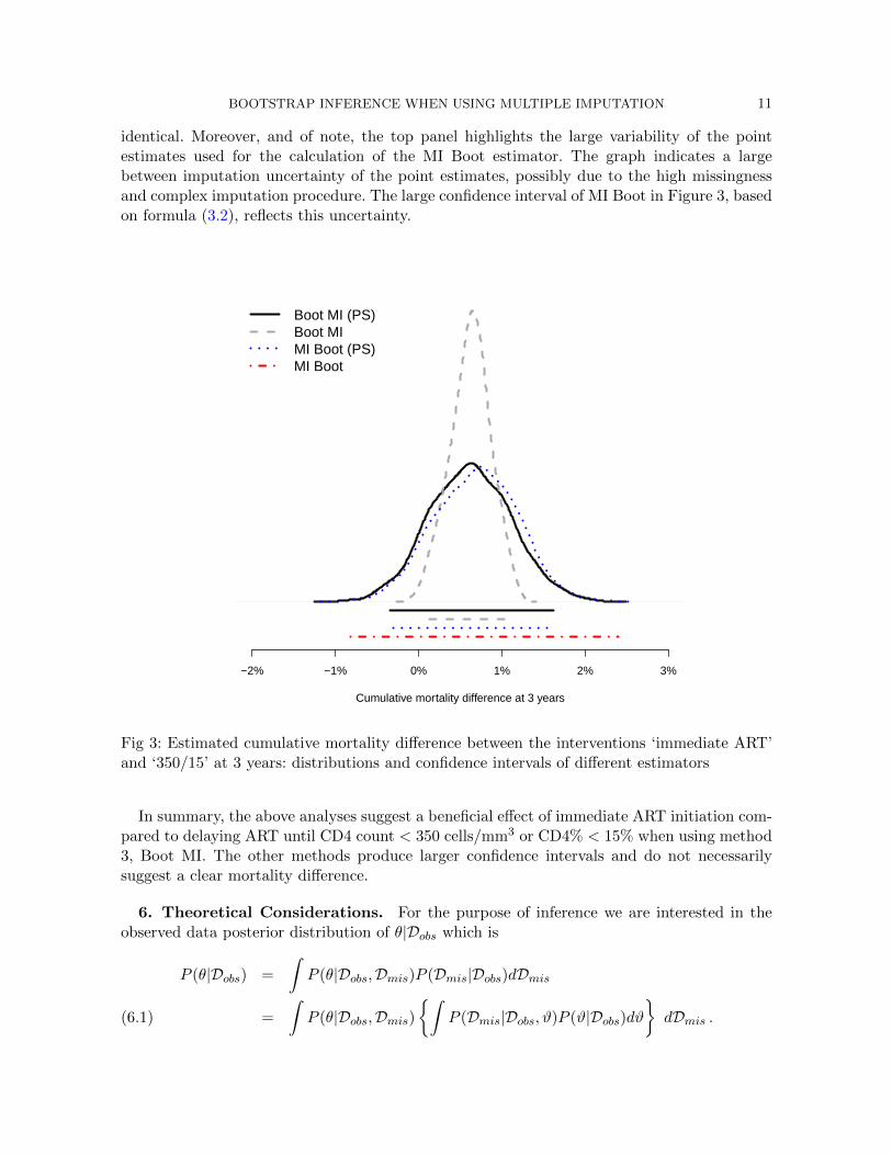
Figure 4 visualizes both the bootstrap distributions in each imputed data set (method MIBoot [PS]) as well as the distribution of the estimators in each bootstrap sample (methodBoot MI [PS]). It is evident that the overall variation of the estimates is similar for these twoapproaches considered, which explains why their confidence intervals in Figure 3 are almost

BOOTSTRAP INFERENCE WHEN USING MULTIPLE IMPUTATION 11

identical. Moreover, and of note, the top panel highlights the large variability of the pointestimates used for the calculation of the MI Boot estimator. The graph indicates a largebetween imputation uncertainty of the point estimates, possibly due to the high missingnessand complex imputation procedure. The large confidence interval of MI Boot in Figure 3, basedon formula (3.2), reflects this uncertainty.

Cumulative mortality difference at 3 years

Boot MI (PS)Boot MIMI Boot (PS)MI Boot

−2% −1% 0% 1% 2% 3%

Fig 3: Estimated cumulative mortality difference between the interventions ‘immediate ART’and ‘350/15’ at 3 years: distributions and confidence intervals of different estimators

In summary, the above analyses suggest a beneficial effect of immediate ART initiation com-pared to delaying ART until CD4 count < 350 cells/mm3 or CD4% < 15% when using method3, Boot MI. The other methods produce larger confidence intervals and do not necessarilysuggest a clear mortality difference.

6. Theoretical Considerations. For the purpose of inference we are interested in theobserved data posterior distribution of θ|Dobs which is

P (θ|Dobs) =

∫P (θ|Dobs,Dmis)P (Dmis|Dobs)dDmis

=

∫P (θ|Dobs,Dmis)

{∫P (Dmis|Dobs, ϑ)P (ϑ|Dobs)dϑ

}dDmis .(6.1)

12

−0.02 −0.01 0.00 0.01 0.02 0.03

020

4060

80

MI Boot (PS)

Distribution of θdiff

Den

sity

−0.02 −0.01 0.00 0.01 0.02 0.03

050

150

250

Boot MI (PS)

Distribution of θdiff

Den

sity

Fig 4: Estimated cumulative mortality difference: distribution of ‘MI Boot (PS)’ for eachimputed dataset (top) and distribution of ‘Boot MI (PS)’ for 25 random bootstrap samples(bottom). Point estimates are marked by the black tick marks on the x-axis.

Please note that ϑ refers to the parameters of the imputation model whereas θ is the quantityof interest from the analysis model. With multiple imputation we effectively approximate theintegral (6.1) by using the average

P (θ|Dobs) ≈1

M

M∑m=1

P (θ|D(m)mis,Dobs)(6.2)

whereD(m)mis refers to draws (imputations) from the posterior predictive distribution P (Dmis|Dobs).

MI Boot and MI Boot (PS). The MI Boot method essentially uses rules (3.1) and (3.2) for

inference, where, for a given scalar, the respective variance in each imputed data set Var(θm) isnot calculated analytically but using bootstrapping. This approach will work if the bootstrapvariance for the imputed data set is close to the analytical variance. If there is no analyticalvariance, it all depends on various factors such as sample size, estimator of interest, proportionof missing data, and others. The data example highlights that in complex settings with a lotof missing data the between imputation variance can be large, yielding conservative interval

BOOTSTRAP INFERENCE WHEN USING MULTIPLE IMPUTATION 13

estimates. As well-known from MI theory M should, in many settings, be much larger than5 for good estimates of the variance [14]. Using bootstrapping to estimate the variance doesnot alter these conclusions. Using MI Boot should always be complemented with a reasonablylarge number of imputations. This consideration also applies to MI Boot pooled, which –asseen in the simulations–, can sometimes be even more sensitive to the choice of M .

Boot MI and Boot MI (PS). Boot MI uses D = {Dmis,Dobs} for bootstrapping. Mostimportantly, we estimate θ, the quantity of interest, in each bootstrap sample using multipleimputation. We therefore approximate P (θ|Dobs) through (6.1) by using multiple imputationto obtain θ and bootstrapping to estimate its distribution – which is valid under the missingat random assumption.

However, if we simply pool the data and apply the method Boot MI (PS) we essentiallypool all estimates θm,b: with this approach each of the B ×M estimates θm,b serves then asan estimator of θ (as we do not combine/average any of them). A possible interpretation ofthis observation is that each θm,b estimates θ and since this is only a single draw from theposterior predictive distribution P (Dmis|Dobs) we conduct multiple imputation with M = 1,

i.e. we calculate ˆθMI = 11

∑1m=1 θm,b, B×M times. Such an estimator is statistically inefficient

as we know from MI theory: the relative efficiency of an MI based estimator (compared to thetrue variance) is (1 + γ

M )−1 where γ describes the fraction of missingness (i.e. V/(W + V ))in the data. For example, if the fraction of missingness is 0.25, and M = 5, then the loss ofefficiency is 5% [6]. The lower M , the lower the efficiency, and thus the higher the variance. Thisexplains the results of the simulation studies: pooling the estimates is inefficient, does thereforeoverestimate the variance, and thus leads to confidence intervals with incorrect coverage.

It follows that one typically gets larger interval estimates when using Boot MI (PS) insteadof Boot MI. Similarly, one can decide to use Boot MI with M = 1, which is not incorrect butoften inefficient in terms of interval estimation.

Comparison. General comparisons between MI Boot and Boot MI are difficult becausethe within and between imputation uncertainty, as well as the within and between bootstrapsampling uncertainty, will determine the actual width of a confidence interval. If the betweenimputation uncertainty is large compared to between bootstrap sample uncertainty (as, forexample, in the data example [Figure 4]) then MI Boot is large compared to Boot MI. However,if the between imputation uncertainty is small relative to the bootstrap sampling uncertainty,then Boot MI may give a similar confidence interval to MI Boot (as in the simulations [Figure2]).

Another consideration is related to the application of the bootstrap. We have focused onthe percentile method to create confidence intervals. However, it is also possible to createbootstrap intervals based on the t−distribution. Here, an estimator’s variance is estimated withthe sample variance from the B bootstrap estimates and symmetric confidence intervals aregenerated based on an appropriate t-distribution. In fact, MI Boot uses this approach because in

each imputed dataset we estimate the bootstrap variance Var(θm) = (B−1)−1∑

b(θm,b−ˆθm,b)

2,then calculate (3.2), followed by confidence intervals based on a tR distribution, see Section 3.A similar approach would be possible when applying Boot MI. This method produces B point

estimates ˆθ∗b = M−1∑

m θ∗b,m for θ. One could estimate the variance as (B−1)−1

∑b(

ˆθ∗b −ˆθ∗)2,

withˆθ∗ = B−1

∑b

ˆθ∗b , and then create confidence intervals based on a t-distribution. This would

14

however require that one assumes the estimator to be approximately normally distributed.

Bootstrapping as part of the imputation procedure. For each of the estimators introducedin Section 3, M proper multiply imputed data sets are needed. “Proper” means that theapplication of formulae (3.1) and (3.2) yield 1) approximately unbiased point estimates and2) interval estimates which are randomization valid in the sense that actual interval coverageequals the nominal interval coverage. Some imputation algorithms use bootstrapping to createproper imputations, and this may not be confused with the bootstrapping step after multipleimputation which we focus on in this paper.

To follow this argument in more detail it is important to understand that proper impu-tations are created by means of random draws from the posterior predictive distribution ofthe missing data given the observed data (or an approximation thereof). These draws can (i)either be generated by specifying a multivariate distribution of the data (joint modeling) andsimulate the posterior predictive distribution with a suitable algorithm; or (ii) by specifyingindividual conditional distributions for each variable Xj given the other variables (fully condi-tional modeling) and iteratively drawing and updating imputed values from these distributionswhich will then (ideally) converge to draws of the theoretical joint distribution; or (iii) by theuse of alternative algorithms.

An example for (i) is the EMB algorithm from the R-package Amelia II which assumes amultivariate normal distribution for the data, D ∼ N(µ,Σ) (possibly after suitable transfor-mations beforehand). Then, B bootstrap samples of the data (including missing values) aredrawn and in each bootstrap sample the EM algorithm [39] is applied to obtain estimatesof µ and Σ which can then be used to generate proper multiple imputations by means of thesweep-operator [40, 11]. Of note, the algorithm can handle highly skewed variables by imposingtransformations on variables (log, square root). Categorical variables are recoded into dummyvariables based on the knowledge that for binary variables the multivariate normal assumptioncan yield good results [9].

An example for (ii) is imputation by chained equations (ICE, mice). Here, (a) one first speci-fies individual conditional distributions (i.e. regression models) p(Xj |X−j , θj) for each variable.Then, (b) one iteratively fits all regression models and generates random draws of the coeffi-

cients, e.g. β ∼ N(β, Cov(β)). Values are (c) imputed as random draws from the distributionof the regression predictions. Then, (b) and (c) are repeated k times until convergence. Theprocess of iteratively drawing and updating the imputed values from the conditional distribu-tions can be viewed as a Gibbs sampler that converges to draws from the (theoretical) jointdistribution. This method is among the most popular ones in practice and has been imple-mented in many software packages [4, 5]. However, there remain theoretical concerns as a jointdistribution may not always exist for a given specifications of the conditional distributions [41].A variation of (c) is a fully Bayesian approach where the posterior predictive distribution isused to draw imputations. Here, the bootstrap is used to model the imputation uncertaintyand to draw the M imputations needed for the M imputed data sets. This variation yieldsapproximate proper imputations and is implemented in the R library Hmisc [42].

An example for (iii) is the Approximate Bayesian Bootstrap [29]. Here, the (cross-sectional)data is stratified into several strata, possibly by means of the covariates of the analysis model.Then, within each stratum (a) one draws a bootstrap sample among the complete data (withrespect to the variable to be imputed). Secondly, (b) one uses the original data set (with missingvalues) and imputes the missing data based on units from the data set created in (a), with

BOOTSTRAP INFERENCE WHEN USING MULTIPLE IMPUTATION 15

equal selection probability and with replacement. The multiply imputed data are obtained byrepeating (a) and (b) M times.

It is evident from the above examples that many imputation methods use bootstrap method-ology as part of the imputation model, that this does not replace the additional bootstrap stepneeded for the inference in the analysis model, and that – if they are combined – the resamplingsteps are nested.

7. Conclusion. The current statistical literature is not clear on how to combine boot-strap with multiple imputation inference. We have proposed that a number of approaches areintuitively appealing and three of them are correct: Boot MI, MI Boot, MI Boot (PS). Us-ing Boot MI (PS) can lead to too large and invalid confidence intervals and is therefore notrecommended.

Both Boot MI and MI Boot are probably the best options to calculate randomization validconfidence intervals when combining bootstrapping with multiple imputation. As a rule ofthumb, our analyses suggest that the former may be preferred for small M or large imputationuncertainty and the latter for normal M and little/normal imputation uncertainty.

There are however other considerations when deciding between MI Boot and Boot MI. Thelatter is computationally much more intensive. This matters particularly when estimating theanalysis model is simple in relation to creating the imputations. In fact, in our first simulationthis affected the computation time by a factor of 13. However, MI Boot naturally provides sym-metrical confidence intervals. These intervals may not be wanted if an estimator’s distributionis suspected to be non-normal.

APPENDIX A: DETAILS OF THE G-FORMULA IMPLEMENTATION

We consider n children studied at baseline (t = 0) and during discrete follow-up times (t =1, . . . , T ). The data consists of the outcome Yt, an intervention variable At, q time-dependentcovariates Lt = {L1

t , . . . , Lqt}, and a censoring indicator Ct. The covariates may also include

baseline variables V = {L10, . . . , L

qV0 }. The treatment and covariate history of an individual i

up to and including time t is represented as At,i = (A0,i, . . . , At,i) and Lst,i = (Ls0,i, . . . , Lst,i)

respectively. Ct equals 1 if a subject gets censored in the interval (t − 1, t], and 0 otherwise.Therefore, Ct = 0 is the event that an individual remains uncensored until time t.

The counterfactual outcome Y at = Y att refers to the hypothetical outcome that would have

been observed at time t if every subject had received, likely contrary to the fact, the treatmenthistory At = at. Similarly, Latt are the counterfactual covariates related to the interventionAt = at. The above notation refers to static treatment rules; a treatment rule may howeverdepend on covariates, and in this case it is called dynamic. A dynamic rule d(at,i; Lt,i) assignstreatment At,i ∈ {0, 1} as a function of the covariate history Lt,i and the intervention vectorat,i may therefore vary by subject i. The counterfactual outcome related to a dynamic rule d is

Yd(at,i;Lt,i)t,i = Y d

t,i, and the counterfactual covariates are Ldt,i. Often At,i = (At,i, Ct,i = 0) which

means that one is interested in the counterfactuals for intervention At,i under (the interventionof) no censoring. In our notation, for simplicity, a rule d can be dynamic and intervene onmultiple variables, including the censoring mechanism, without referring to it explicitly, i.e. dmay relate to d(at,i, ct,i; Lt,i). We write adt,i for the intervention history individual i received

under rule d.In our setting we study n = 5826 children for t = 0, 1, 3, 6, 9, . . . where the follow-up time

16

points refer to the intervals (0, 1.5), [1.5, 4.5), [4.5, 7.5), . . ., [28.5, 31.5), [31.5, 36) months re-spectively. Follow-up measurements, if available, refer to measurements closest to the middle ofthe interval. In our data Yt refers to death at time t (i.e. occurring during the interval (t−1, t]).At refers to antiretroviral treatment (ART) taken at time t. Lt = (L1

t , L2t , L

3t , L

1mt , L2m

t , L3mt )

are CD4 count, CD4%, and weight for age z-score (WAZ, which serves as a proxy for WHOstage, see [43] for more details) as well as three indicator variables whether these variableshave been measured at time t or not. V = LV0 refer to baseline values of CD4 count, CD4%,WAZ, height for age z-score (HAZ) as well as sex, age, and region. The two treatment rules ofinterest are:

d1t,i =

{ct,i = 0; l1mt,i = l2mt,i = l3mt,i = 1; at,i = 1 for ∀t, i

d2t,i =

{ct,i = 0; l1mt,i = l2mt,i = l3mt,i = 1; at,i = 1 if CD4 countdt,i < 350 or CD4%d

t,i < 15%

ct,i = 0; l1mt,i = l2mt,i = l3mt,i = 1; at,i = 0 otherwise

The quantity of interest is thus cumulative mortality after T = 36 months, under (the inter-vention of) no censoring, regular 3 monthly follow-up and for treatment assignment accordingto dj , that is ψ =

∑Tt=1 P(Y d

t = 1).

Under the assumption of consistency, i.e. Y d = Y if At = adt,i and Ldt = Lt if At−1 = adt−1,i,

sequential conditional exchangeability (or no unmeasured confounding), i.e. Y d∐At|Lt, At−1

for ∀At = adt , Lt = lt, t ∈ {0, . . . , T} and positivity, i.e. P (At = adt |Lt = lt, At−1 = adt−1) > 0 for

∀t, adt , lt with P (Lt = lt, At−1 = adt−1) 6= 0, the g-computation formula can estimate ψ as:

ψ =T∑t=1

P(Y dt = 1) =

T∑t=1

∫l∈Lt

P(Yt = 1|At−1 = adt−1,i, Lt = lt, Yt−1 = 0)×T∏t=1

f(Lt|At−1 = adt−1,i, Lt−1 = lt−1, Yt−1 = 0)

dl(A.1)

see [23] and [44] about more details and implications of the representation of the g-formula inthis context. Note that the inner product of (A.1) can be written as

T∏t=1

q∏s=1

f(Lst |At−1= adt−1,i, Lt−1= lt−1,L1t= l1t , . . . , L

s−1t = ls−1

t , Yt−1= 0) .

In the above representation of the g-formula we assume that the time ordering is L1t → L2

t →L3t → A/C → Y .There is no closed form solution to estimate (A.1), but θ can be approximated by means of

the following algorithm; Step 1: use additive linear and logistic regression models to estimate theconditional densities on the right hand side of (A.1), i.e. fit regression models for the outcomevariables CD4 count, CD4%, WAZ, and death at t = 1, 3, .., 36 using the available covariatehistory and model selection. Step 2: use the models fitted in step 1 to stochastically generateLt and Yt under a specific treatment rule. For example, for rule (ii), draw L1

1 =√

CD4 count1

from a normal distribution related to the respective additive linear model from step 1 usingthe relevant covariate history data. Set A1 = 1 if the generated CD4 count at time 1 is < 350cells/mm3 or CD4% < 15% (for rule d2). Use the simulated covariate data and treatmentas assigned by the rule to generate the full simulated data set forward in time and evaluate

BOOTSTRAP INFERENCE WHEN USING MULTIPLE IMPUTATION 17

cumulative mortality after 3 years of follow-up. We refer the reader to [17], [23], and [44] tolearn more about the g-formula in this context.

Note that the so-called sequential g-formula, used in the simulation study, shares the ideaof standardization in the sense that one sequentially marginalizes the distribution with respectto L given the intervention rule of interest. It is just a re-expression of (A.1) where integrationwith respect L is not needed [45]:

E(Y dT ) = E(E( . . .E(E(YT |AT = adT , LT )|AT−1 = adT−1, LT−1 ) . . . |A0 = ad0, L0 )|L0 ) .(A.2)

APPENDIX B: DATA GENERATING PROCESS IN THE SIMULATION STUDY

Both baseline data (t = 0) and follow-up data (t = 1, . . . , 12) were created using struc-tural equations using the R-package simcausal [34]. The below listed distributions, listed intemporal order, describe the data-generating process. Baseline data refers to region, sex, age,CD4 count, CD4%, WAZ and HAZ respectively (V 1, V 2, V 3, L1

0, L20, L3

0, Y0). Follow-up datarefers to CD4 count, CD4%, WAZ and HAZ (L1

t , L2t , L

3t , Yt), as well as an antiretroviral treat-

ment (At) and censoring (Ct) indicator. For simplicity, no deaths are assumed. In additionto Bernoulli (B), uniform (U) and normal (N) distributions, we also use truncated normaldistributions which are denoted by N[a,b] where a and b are the truncation levels. Values whichare smaller a are replaced by a random draw from a U(a1, a2) distribution and values greaterthan b are drawn from a U(b1, b2) distribution. Values for (a1, a2, b1, b2) are (0, 50, 5000, 10000)for L1, (0.03, 0.09, 0.7, 0.8) for L2, and (−10, 3, 3, 10) for both L3 and Y . The notation D means“conditional on the data that has already been measured (generated) according the the timeordering”. The distributions are listed in Figure 5

The data generating process leads to the following baseline values: region A = 75.5%; malesex = 51.2%; mean age = 3.0 years; mean CD4 count = 672.5; mean CD4% = 15.5%; meanWAZ = -1.5; mean HAZ = -2.5. At t = 12 the arithmetic mean of CD4 count, CD4%, WAZand HAZ are 1092, 27.2%, -0.8, -1.5 respectively. The target quantities ψ1 and ψ2 are definedas the expected value of Y at time T , under no censoring, for a given treatment rule dj , where

d1t,i = {ct,i = 0; at,i = 1 for ∀t, i and d2

t,i = {ct,i = 0; at,i = 0 for ∀t, i

and are −1.03 and −2.45 respectively. Missing baseline and follow-up data were created basedon the following functions:

π(L1t ) = 0.1;

π(L20)(L

10) = 1− 1

(0.001 · L10)2 + 1

; π(L2t )(t, L

1t ) = 1− 1

(0.00005 · t · L1t )

2 + 1;

π(L30)(Y0) = 1− 1

(0.2 · |Y0|)2 + 1; π(L3

t )(t, Yt) = 1− 1

(0.015 · t · |Yt|)2 + 1;

π(Y0)(L30) = 1− 1

(0.7 · |L30|)2 + 1

; π(Yt)(t, L3t ) = 1− 1

(0.015 · t · |L3t |)2 + 1

.

18

V1∼

B(p

=4392/5826)

V2|D

∼{B

(p=

2222/4392)

ifV

1=

1B

(p=

758/1434)

ifV

1=

0

V3|D

∼U

(1,5

)

L10 |D

∼{

N[0,10000] (6

50,3

50)

ifV

1=

1N

[0,10000] (7

20,4

00))

ifV

1=

0

L10 |D

∼N

((L10 −

671.7

468)/

(10·

352.2

788)

+1,0

)

L20 |D

∼N

[0.06,0.8] (0.1

6+

0.0

5·(L

10 −650)/

650,0.0

7)

L20 |D

∼N

((L20 −

0.1

648594)/

(10·

0.0

6980332)

+1,0

)

L30 |D

∼{

N[−

5,5] (−

1.6

5+

0.1·

V3

+0.0

5·(L

10 −650)/

650

+0.0

5·(L

20 −16)/

16,1

)if

V1

=1

N[−

5,5] (−

2.0

5+

0.1·

V3

+0.0

5·(L

10 −650)/

650

+0.0

5·(L

20 −16)/

16,1

))if

V1

=0

A0 |D

∼B

(p=

0)

C0 |D

∼B

(p=

0)

Y0 |D

∼N

[−5,5] (−

2.6

+0.1·

I(V

3>

2)

+0.3·

I(V

1=

0)

+(L

30+

1.4

5),1

.1)

L1t |D

∼

N

[0,10000] (1

3·lo

g(t·

(1034−

662)/

8)

+L

1t−1

+2·L

2t−1

+2·L

3t−1

+2.5·

At−

1 ,50)

ift∈{1,2,3,4}

N[0,10000] (4·

log(t·

(1034−

662)/

8)

+L

1t−1

+2·L

2t−1

+2·L

3t−1

+2.5·

At−

1 ,50)

ift∈{5,6,7,8}

N[0,10000] (L

1t−1

+2·L

2t−1

+2·L

3t−1

+2.5·

At−

1 ,50)

ift∈{9,1

0,1

1,1

2}L

2t |D∼

N[0.06,0.8] (L

2t−1

+0.0

003·

(L1t −

L1t−

1 )+

0.0

005·

(L3t−

1 )+

0.0

005·A

t−1 ·L

10 ,0.0

2)

L3t |D

∼N

−5,5 (L

3t−1

+0.0

017·

(L1t −

L1t−

1 )+

0.2·

(L2t −

L2t−

1 )+

0.0

05·A

t−1 ·L

20 ,0.5

)

At |D

∼{

B(p

=1)

ifA

t−1

=1

B(p

=1/(1

+ex

p(−

[−2.4

+0.0

15·

(750−

L1t )

+5·

(0.2−

L2t )−

0.8·

L3t

+0.8·

t])))if

At−

1=

0

Ct |D

∼B

(p=

1/(1

+ex

p(−

[−6

+0.0

1·(7

50−

L1t )

+1·

(0.2−

L2t )−

0.6

5·L

3t −A

t ])))

Yt |D

∼N

[−5,5] (Y

t−1

+0.0

0005·

(L1t −

L1t−

1 )−0.0

00001· (

(L1t −

L1t−

1 )· √L

10 )2

+0.0

1·(L

2t −L

2t−1 )−

0.0

001· (

(L2t −

L2t−

1 )· √L

20 )2

+0.0

7·((L

3t −L

3t−1 )·

(L30

+1.5

135))−

0.0

01·

((L3t −

L3t−

1 )·(L

30+

1.5

135))

2+

0.0

05·A

t+

0.0

75·A

t−1

+0.0

5·A

[t]·A

[t−1],0.0

1)

Fig

5:D

atagen

erating

pro

cessin

the

simu

lationstu

dy

BOOTSTRAP INFERENCE WHEN USING MULTIPLE IMPUTATION 19

ACKNOWLEDGEMENTS

The authors gratefully acknowledge Mary-Ann Davies and Valeriane Leroy who contributedto the analysis and study design of the data analysis. We further thank Lorna Renner, ShobnaSawry, Sylvie N’Gbeche, Karl-Gunter Technau, Francois Eboua, Frank Tanser, Haby Sygnate-Sy, Sam Phiri, Madeleine Amorissani-Folquet, Vivian Cox, Fla Koueta, Cleophas Chimbete,Annette Lawson-Evi, Janet Giddy, Clarisse Amani-Bosse, and Robin Wood for sharing theirdata with us. We would also like to highlight the support of the Pediatric West African Groupand the Paediatric Working Group Southern Africa. The NIH has supported the above indi-viduals, grant numbers 5U01AI069924-05 and U01AI069919. We also thank Jonathan Bartlettfor his feedback on an earlier version of this paper.

REFERENCES

[1] D. B. Rubin. Multiple imputation after 18+ years. Journal of the American Statistical Association,91(434):473–489, 1996.

[2] N. J. Horton and K. P. Kleinman. Much ado about nothing: a comparison of missing data methods andsoftware to fit incomplete regression models. The American Statistician, 61:79–90, 2007.

[3] J. Honaker, G. King, and M. Blackwell. Amelia II: A program for missing data. Journal of StatisticalSoftware, 45(7):1–47, 2011.

[4] S. van Buuren and K. Groothuis-Oudshoorn. mice: Multivariate imputation by chained equations in R.Journal of Statistical Software, 45(3):1–67, 2011.

[5] P. Royston and I. R. White. Multiple imputation by chained equations (mice): Implementation in Stata.Journal of Statistical Software, 45(4):1–20, 2011.

[6] I. R. White, P. Royston, and A. M. Wood. Multiple imputation using chained equations. Statistics inmedicine, 30:377–399, 2011.

[7] J. A. C. Sterne, I. R. White, J. B. Carlin, M. Spratt, P. Royston, M. G. Kenward, A. M. Wood, and J. R.Carpenter. Multiple imputation for missing data in epidemiological and clinical research: potential andpitfalls. British Medical Journal, 339, 2009.

[8] J. W. Graham. Missing data analysis: Making it work in the real world. Annual Review of Psychology,60:549–576, 2009.

[9] J. Schafer and J. Graham. Missing data: our view of the state of the art. Psychological Methods, 7:147–177,2002.

[10] W. Eddings and Y. Marchenko. Diagnostics for multiple imputation in Stata. Stata Journal, 12(3):353–367,2012.

[11] J. Honaker and G. King. What to do about missing values in time-series cross-section data? AmericanJournal of Political Science, 54:561–581, 2010.

[12] B. Efron. Missing data, imputation, and the bootstrap. Journal of the American Statistical Association,89(426):463–475, 1994.

[13] J. Shao and R. R. Sitter. Bootstrap for imputed survey data. Journal of the American Statistical Associ-ation, 91(435):1278–1288, 1996.

[14] R. Little and D. Rubin. Statistical analysis with missing data. Wiley, New York, 2002.[15] A. H. Briggs, G. Lozano-Ortega, S. Spencer, G. Bale, M. D. Spencer, and P. S. Burge. Estimating the cost-

effectiveness of fluticasone propionate for treating chronic obstructive pulmonary disease in the presenceof missing data. Value in Health, 9(4):227–235, 2006.

[16] M. Schomaker and C. Heumann. Model selection and model averaging after multiple imputation. Compu-tational Statistics & Data Analysis, 71:758–770, 2014.

[17] M. Schomaker, M. A. Davies, K. Malateste, L. Renner, S. Sawry, S. N’Gbeche, K. Technau, F. T. Eboua,F. Tanser, H. Sygnate-Sy, S. Phiri, M. Amorissani-Folquet, V. Cox, F. Koueta, C. Chimbete, A. Lawson-Evi, J. Giddy, C. Amani-Bosse, R. Wood, M. Egger, and V. Leroy. Growth and mortality outcomes fordifferent antiretroviral therapy initiation criteria in children aged 1-5 years: A causal modelling analysisfrom West and Southern Africa. Epidemiology, 27:237–246, 2016.

[18] H. Worthington, R. King, and S. T. Buckland. Analysing mark-recapture-recovery data in the presenceof missing covariate data via multiple imputation. Journal of Agricultural, Biological, and EnvironmentalStatistics, 20:28, 2015.

20

[19] W. Wu and F. Jia. A new procedure to test mediation with missing data through nonparametric boot-strapping and multiple imputation. Multivariate Behavioral Research, 48(5):663–691, 2013.

[20] M. R. Baneshi and A. Talei. Assessment of internal validity of prognostic models through bootstrappingand multiple imputation of missing data. Iranian Journal of Public Health, 41(5):110–115, 2012.

[21] M. W. Heymans, S. van Buuren, D. L. Knol, W. van Mechelen, and H. C. W. de Vet. Variable selectionunder multiple imputation using the bootstrap in a prognostic study. BMC Medical Research Methodology,7, 2007.

[22] B. W. Chaffee, C. A. Feldens, and M. R. Vitolo. Association of long-duration breastfeeding and dentalcaries estimated with marginal structural models. Annals of Epidemiology, 24(6):448–454, 2014.

[23] D. Westreich, S. R. Cole, J. G. Young, F. Palella, P. C. Tien, L. Kingsley, S. J. Gange, and M. A. Hernan.The parametric g-formula to estimate the effect of highly active antiretroviral therapy on incident AIDSor death. Statistics in medicine, 31(18):2000–2009, 2012.

[24] A. Edmonds, M. Yotebieng, J. Lusiama, Y. Matumona, F. Kitetele, S. Napravnik, S. R. Cole, A. Van Rie,and F. Behets. The effect of highly active antiretroviral therapy on the survival of HIV-infected childrenin a resource-deprived setting: a cohort study. PLoS Medicine, 8(6):e1001044, 2011.

[25] A. Violari, M. F. Cotton, D. M. Gibb, A. G. Babiker, J. Steyn, S. A. Madhi, P. Jean-Philippe, and J. A.McIntyre. Early antiretroviral therapy and mortality among HIV-infected infants. New England Journalof Medicine, 359(21):2233–2244, 2008.

[26] R. M. Daniel, S. N. Cousens, B. L. De Stavola, M. G. Kenward, and J. A. Sterne. Methods for dealingwith time-dependent confounding. Statistics in Medicine, 32(9):1584–618, 2013.

[27] M. Petersen, J. Schwab, S. Gruber, N. Blaser, M. Schomaker, and M. van der Laan. Targeted maximumlikelihood estimation for dynamic and static longitudinal marginal structural working models. Journal ofCausal Inference, 2:147–185, 2014.

[28] J. Robins. A new approach to causal inference in mortality studies with a sustained exposure period -application to control of the healthy worker survivor effect. Mathematical Modelling, 7(9-12):1393–1512,1986.

[29] D. Rubin and N. Schenker. Multiple imputation for interval estimation from simple random samples withignorable nonresponse. Journal of the American Statistical Association, 81:366–374, 1986.

[30] S. Lipsitz, M. Parzen, and L. Zhao. A degrees-of-freedom approximation in multiple imputation. Journalof Statistical Computation and Simulation, 72:309–318, 2002.

[31] J. Robins and M. A. Hernan. Estimation of the causal effects of time-varying exposures, pages 553–599.CRC Press, 2009.

[32] J. Yan. Enjoy the joy of copulas: with package copula. Journal of Statistical Software, 21:1–21, 2007.[33] M. Schomaker, S. Hogger, L. F. Johnson, C. Hoffmann, T. Brnighausen, and C. Heumann. Simultane-

ous treatment of missing data and measurement error in HIV research using multiple overimputation.Epidemiology, 26:628–636, 2015.

[34] Oleg Sofrygin, Mark J. van der Laan, and Romain Neugebauer. simcausal: Simulating Longitudinal Datawith Causal Inference Applications, 2016. R package version 0.5.3.

[35] J. M. Robins, A. Rotnitzky, and L. P. Zhao. Estimation of regression-coefficients when some regressors arenot always observed. Journal of the American Statistical Association, 89(427):846–866, 1994.

[36] R. J. A. Little. Regression with missing X’s - a review. Journal of the American Statistical Association,87(420):1227–1237, 1992.

[37] M. Egger, D. K. Ekouevi, C. Williams, R. E. Lyamuya, H. Mukumbi, P. Braitstein, T. Hartwell, C. Graber,B. H. Chi, A. Boulle, F. Dabis, and K. Wools-Kaloustian. Cohort profile: The international epidemiolog-ical databases to evaluate AIDS (IeDEA) in sub-Saharan Africa. International Journal of Epidemiology,41(5):1256–1264, 2012.

[38] D. K. Ekouevi, A. Azondekon, F. Dicko, K. Malateste, P. Toure, F. T. Eboua, K. Kouadio, L. Renner,K. Peterson, F. Dabis, H. S. Sy, and V. Leroy. 12-month mortality and loss-to-program in antiretroviral-treated children: The iedea pediatric west african database to evaluate aids (pwada), 2000-2008. BmcPublic Health, 11:519, 2011.

[39] A. Dempster, N. Laird, and D. Rubin. Maximum likelihood from incomplete data via the em algorithm.Journal of the Royal Statistical Society B, 39:1–38, 1977.

[40] J. H. Goodnight. Tutorial on the sweep operator. American Statistician, 33(3):149–158, 1979.[41] J. Drechsler and S. Rssler. Does convergence really matter?, pages 342–355. Springer, 2008.[42] Frank E Harrell Jr, with contributions from Charles Dupont, and many others. Hmisc: Harrell Miscella-

neous, 2016. R package version 4.0-1.

BOOTSTRAP INFERENCE WHEN USING MULTIPLE IMPUTATION 21

[43] M. Schomaker, M. Egger, J. Ndirangu, S. Phiri, H. Moultrie, K. Technau, V. Cox, J. Giddy, C. Chimbetete,R. Wood, T. Gsponer, C. Bolton Moore, H. Rabie, B. Eley, L. Muhe, M. Penazzato, S. Essajee, O. Keiser,and M. A. Davies. When to start antiretroviral therapy in children aged 2-5 years: a collaborative causalmodelling analysis of cohort studies from southern Africa. Plos Medicine, 10(11):e1001555, 2013.

[44] J. G. Young, L. E. Cain, J. M. Robins, E. J. O’Reilly, and M. A. Hernan. Comparative effectiveness ofdynamic treatment regimes: an application of the parametric g-formula. Statistics in biosciences, 3(1):119–143, 2011.

[45] M. L. Petersen. Commentary: Applying a causal road map in settings with time-dependent confounding.Epidemiology, 25(6):898–901, 2014.

Michael SchomakerCentre for Infectious Disease Epidemiology & ResearchUniversity of Cape TownCape Town, South AfricaE-mail: michael.schomaker@uct.ac.za

Christian HeumannInstitut fur StatistikLudwig-Maximilians Universitat MunchenMunchen, GermanyE-mail: chris@stat.uni-muenchen.de