Bayesian Inference andthe Parametric Bootstrap

Bradley Efron

Stanford University

Importance Sampling for Bayes Posterior Distribution

• Newton and Raftery (1994 JRSS-B)

“Nonparametric Bootstrap: good choice”

(actually used a smoothed nonparametric bootstrap)

• Today Parametric Bootstrap

– Good computational properties when applicable

– Connection between Bayes and frequentist inference

Bayesian Inference 1

Student Score Data

(Mardia, Kent and Bibby)

• n = 22 students’ scores on two tests: mechanics, vectors

• Data y = (y1, y2, . . . , y22) with yi = (meci, veci)

• Parameter of interest θ = correlation (mec, vec)

• Sample correlation coefficient θ = 0.498± ??

Bayesian Inference 2

●

●

●

●

●

●●

●

●

●

●

●●

●

●

●

●

●

●

●

●

●

0 20 40 60

3040

5060

70

Scores of 22 students on two tests 'mechanics' and 'vectors';Sample Correlation Coefficient is .498 +−??

Sampled from 88 students, Mardia, Kent and Bibbymechanics score

vect

ors

scor

e

Bayesian Inference 3

R. A. Fisher (1915)

• Density fθ(θ)

=n − 2π

(1−θ2)(n−1)/2(1 − θ2

)(n−4)/2∫∞

0

[cosh(w) − θθ

]−(n−1)dw

• Bivariate normal yiind∼ N2(µ, /Σ) i = 1, 2, . . . ,n

• 95% confidence limits (from z transform)

θ ∈ (0.084, 0.754)

Bayesian Inference 4

Fisher density for correlation coefficient if corr=.498And histogram for 10000 parametric bootstrap replications

Red triangles are Fisher 95% confidence limitscorrelation

Fre

quen

cy

−0.2 0.0 0.2 0.4 0.6 0.8 1.0

010

020

030

040

050

060

0

corrhat=.498.084 .754

0.5−

1 −

1.5−

2 −

2.5−

density

Bayesian Inference 5

Parametric Bootstrap Computations

• Assume yiind∼ N2(µ, /Σ) • Estimate µ and /Σ by MLE

• Bootstrap sample y∗iind∼ N2

(µ, /Σ

)for i = 1, 2, . . . , 22

• Bootstrap replication θ∗ = corr coeff for y∗ = (y∗1, y∗

2, . . . , y∗

22)

• Bootstrap standard deviation

sd(θ)

= 0.168 (B = 10, 000)

• Percentile 95% confidence limits (0.109, 0.761)

Bayesian Inference 6

Better Bootstrap Confidence Limits (BCa)

• Idea Reweighting the B bootstrap replications

improves coverage

• Weights involve z0 (bias correction) and a (acceleration)

• WBCa(θ) =ϕ(Zθ/(1 + aZθ) − z0)(1 + aZθ)2ϕ(Zθ + z0)

where Zθ = Φ−1G(θ) − z0

↑

bootstrap cdf

• Reweighting the B = 10, 000 bootstraps

gave weighted percentiles

(0.075, 0.748) Fisher: (0.084, 0.754)

Bayesian Inference 7

Bayes Posterior Intervals

• Prior π(θ) • Posterior expectation for t(θ):

E{t(θ)|θ

}=

∫t(θ)π(θ) fθ

(θ)

dθ/∫

π(θ) fθ(θ)

dθ

• Conversion factor Ratio of likelihood to bootstrap density:

R(θ) = fθ(θ) /

fθ(θ)(“θ” = θ∗

)• Bootstrap integrals

E{t(θ)|θ

}=

∫t(θ)π(θ)R(θ) fθ(θ) dθ∫π(θ)R(θ) fθ(θ) dθ

Bayesian Inference 8

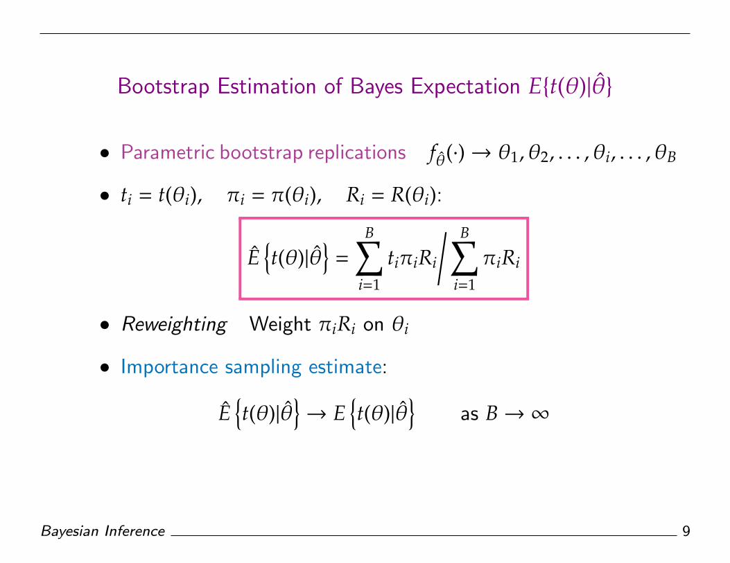
Bootstrap Estimation of Bayes Expectation E{t(θ)|θ}

• Parametric bootstrap replications fθ(·)→ θ1, θ2, . . . , θi, . . . , θB

• ti = t(θi), πi = π(θi), Ri = R(θi):

E{t(θ)|θ

}=

B∑i=1

tiπiRi

/ B∑i=1

πiRi

• Reweighting Weight πiRi on θi

• Importance sampling estimate:

E{t(θ)|θ

}→ E

{t(θ)|θ

}as B→∞

Bayesian Inference 9

Jeffreys Priors

• Harold Jeffreys (1930s):

Theory of “uninformative” prior distributions

(“invariant”, “objective”, “reference”, . . . )

• For density family fθ(y), θ ∈ Rp:

π(θ) = c|I(θ)|1/2 I(θ) = Fisher info matrix

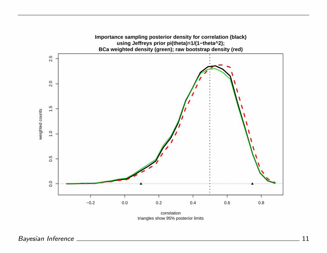
• Normal correlation π(θ) = 1/(1 − θ2)

Bayesian Inference 10

−0.2 0.0 0.2 0.4 0.6 0.8

0.0

0.5

1.0

1.5

2.0

2.5

Importance sampling posterior density for correlation (black)using Jeffreys prior pi(theta)=1/(1−theta^2);

BCa weighted density (green); raw bootstrap density (red)

triangles show 95% posterior limitscorrelation

wei

ghte

d co

unts

Bayesian Inference 11

Multiparameter Exponential Families RP

• p-dimensional sufficient statistic β

• p-dimensional parameter vector β = E{β}

(Poisson: e−λλx/x! has β = x, β = λ)

• Hoeffding fβ(β)

= fβ(β)

e−D(β,β)/2

• Deviance D(β1, β2) = 2Eβ1 log{

fβ1

(β) /

fβ2

(β)}

Bayesian Inference 12

Conversion Factor in Exponential Families

• Conversion factor R(β) = fβ(β) /

fβ(β) (with β fixed)

R(β) = ν(β)e∆(β)

where ∆(β) =[D

(β, β

)−D

(β, β

)] /2

• ν(β) = fβ(β) /

fβ(β) � 1/Jeffreys prior (Laplace)

• Jeffreys prior π(β)R(β) � e∆(β)

Bayesian Inference 13

Example: Multivariate Normal

• yiind∼ Nd(µ,Σ) for i = 1, 2, . . . ,n

• ∆ =

n

(µ − µ)′ /Σ−1− /Σ−1

2(µ − µ

)+

12

tr(/Σ/Σ−1− /Σ/Σ−1

)+ log

|/Σ|

|/Σ|

• “eigenratio” (student score data)

• θ =λ1

λ1 + λ2• θ =

λ1

λ1 + λ2= 0.793± ??

• Bootstrap y∗iind∼ Nd

(µ, /Σ

)i = 1, 2, . . . ,n→ θ1, θ2, . . . , θB

Bayesian Inference 14

0.5 0.6 0.7 0.8 0.9

01

23

45

67

Density estimates for student score eigenratio (B=10,000);Boot (red),Jeffreys (5−dim prior) Black, and BCa Green (z0=−.182, a=0)

Triangles show 95% limits: bca (.598,.890) bayes (.650,.908)eigenratio

dens

ity

BCa

Jeffreys

boot

Bayesian Inference 15

*

*

**

*

*

*

*

*

*

*

**

*

**

*

*

*

*

*

*

* *

*

*

*

*

*

**

*

*

*

**

*

*

**

*

*

**

*

***

*

**

*

*

*

*

*

*

*

*

*

*

**

*

*

*

*

*

*

*

*

*

*

*

*

* *

**

*

*

*

*

*

*

*

*

*

* **

*

*

*

*

*

*

*

*

*

**

*

**

*

*

*

**

*

*

*

*

*

*

*

*

*

*

*

*

*

*

*

*

*

**

*

*

**

*

*

**

**

*

*

*

**

**

*

*

** *

*

*

*

*

** *

*

*

*

*

*

*

*

*

*

*

*

**

*

*

*

*

** *

*

* *

*

*

*

**

* * *

*

*

*

*

*

*

*

* *

*

*

*

*

*

**

*

*

*

*

*

*

*

**

*

*

**

*

*

**

*

*

*

*

*

*

*

*

*

*

*

*

*

*

*

*

*

**

**

*

**

*

*

*

*

−3 −2 −1 0 1 2 3

−3

−2

−1

01

23

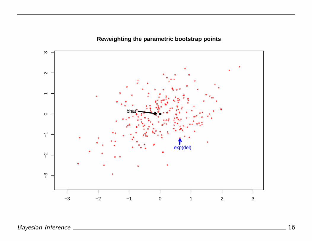
Reweighting the parametric bootstrap points

●bhat

exp(del)

Bayesian Inference 16

Prostate Cancer Study

(Singh et al, 2002)

• Microarray study

102 men: 52 prostate cancer, 50 healthy controls

• 6033 genes zi test statistic for H0i: “no difference”

H0i : zi ∼ N(0, 1)

• Goal Identify genes involved in prostate cancer

Bayesian Inference 17

Prostate cancer z−values for 6033 genes; 52 patients vs50 healthy controls. N(0,1) black; LogPoly4 red

z value

coun

ts

−4 −2 0 2 4

010

020

030

040

0

log poly4 fit

Bayesian Inference 18

Poisson Regression Models

• Histogram y j = #{zi ∈ bin j}

• x j = midpoint bin j, j = 1, 2, . . . , J

• Poisson model y jind∼ Poi(µ j)

with log(µ j) = poly(x j, degree = m)

• Exponential family degree p = m+1 • Let η j = log(µ j)

∆ = (η − η)′ (µ + µ) − 2(∑

µ j −∑µ j

)

Bayesian Inference 19

Parametric False Discovery Rate Estimates

• glm(y∼poly(x,4),Poisson) −→{µ j

}(“log poly 4”)

• θ = Fdr(3) = [1 −Φ(3)]/ [

1 − F(3)]≈ Pr{null|z ≥ 3}

(F is smoothed CDF estimate)

• Model 4: Fdr(3) = 0.192± ??

• Parametric bootstrap y∗jind∼ Poi

(µ j

)→

{µ∗j

}→ Fdr(3)∗

Bayesian Inference 20

0.15 0.20 0.25 0.30

05

1015

20

Fdr(3) estimation, Model 4; prostate data from 4000 parboots;Jeffreys Bayes (black), raw boot (red), bca (green)

triangles show 95% Jeffreys/BCa limits (.154, .241)Fdr(3)*

post

erio

r de

nsity

Bayesian Inference 21

Compare Model 4 (line) with Model 8 (solid);4000 parametric bootstrap replications of Fdr(3)

triangles are 95% bca limits: (.141,.239) vs (.154,.241)Fdr(3) bootreps

coun

ts

0.15 0.20 0.25 0.30

050

100

150

200

250

300

Bayesian Inference 22

Model Selection: AIC = Deviance + 2 · df

Model AIC boot counts Bayes counts†

M2 142.6 0 0.0

M3 143.1 0 0.0

M4 73.3 1266 1458 (36%)

M5 74.3 415 462 (12%)

M6 75.8 215 197 (5%)

M7 77.8 54 67 (2%)

M8 75.6 2050 1816 (45%)

† Model 8, Jeffreys prior

Bayesian Inference 23

Internal Accuracy of Bayes Estimates

• B for computing E{t(β)|β

}=

B∑1

tiπiRi

/ B∑1

πiRi ?

• Define ri = πiRi and si = tiπiRi • css =

B∑1

(si−s)2/B, etc.

CV{E}2

=1B

( css

s2 − 2csr

sr+

crr

r2

)• Example t = Fdr(3)

4000 parametric bootreps, Jeffreys Bayes

• Model 4 E = 0.193 CV = 0.0019

• Model 8 E = 0.179 CV = 0.0025

Bayesian Inference 24

Sampling Variability of Bayes Estimates

• How much would E{t(β)|β

}vary for new β’s?

(i.e., frequentist properties of Bayes estimates)

• Need to bootstrap the parametric bootstrap calculations

for E{t(β)|β

}• Shortcut “Bootstrap after bootstrap”

Bayesian Inference 25

Bootstrap-after-Bootstrap Calculations

• fβ(·) −→ β1, β2, . . . , βi, . . . , βB,

the original bootstrap reps under β

• Want bootreps under some other value γ

• Idea Reweight the originals

• Weight Qγ(β) = fβ(γ)/ fβ

(β):

E{t|γ

}=

B∑1

tiπiRiQγ(βi)/ B∑

1

πiRiQγ(βi)

Bayesian Inference 26

Bootstrap-after-Bootstrap Standard Errors

• BAB

fβ(·)→ γ1, γ2, . . . , γk(1)

Ek = E{t|γk

}(2)

se{E}

=[∑(

Ek − E·)2 /

K]1/2

(3)

• Example Model 4

97.5% credible limit for Fdr(3) = 0.241± ??

Bayesian Inference 27

400 BAB replications of 97.5% credible upper limit for Fdr(3);line histogram: same for BCa upper limit

BAB Standard Errors: .030 (Bayes) .034 (BCa); corr .9897.5% credible upper limit

Fre

quen

cy

0.18 0.20 0.22 0.24 0.26 0.28 0.30 0.32

010

2030

40

.240

Bayesian Inference 28

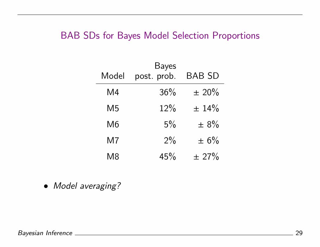
BAB SDs for Bayes Model Selection Proportions

BayesModel post. prob. BAB SD

M4 36% ± 20%

M5 12% ± 14%

M6 5% ± 8%

M7 2% ± 6%

M8 45% ± 27%

• Model averaging?

Bayesian Inference 29

A Few Conclusions . . .

• Parametric bootstrap closely related to objective Bayes.

(That’s why it’s a good importance sampling choice.)

• When it applies, parboot approach has both computational

and interpretational advantages over MCMC/Gibbs.

• Objective Bayes analyses should be checked frequentistically.

Bayesian Inference 30

References

• Bootstrap DiCiccio & Efron 1996 Statist. Sci. 189–228

• Bayes and Bootstrap Newton & Raftery 1994 JRSS-B

3–48 (see Discussion!)

• Objective Priors Berger & Bernardo 1989 JASA 200–207;

Ghosh 2011 Statist. Sci. 187–202

• Exponential Families Efron 2010 Large-Scale Inference,

Appendix 1

• MCMC and Bootstrap Efron 2011 J. Biopharm. Statist.

1052–1062

Bayesian Inference 31