bond options, caps and the black model · bond options, caps and the black model. black formula ......
TRANSCRIPT

Bond Options, Caps and the Black Model

Black formula
• Recall the Black formula for pricing options on futures:
C (F ,K , σ, r ,T , r) = Fe−rTN(d1)− Ke−rTN(d2)
where
d1 =1
σ√
T
[ln(
F
K) +
1
2σ2T
]d2 = d1 − σ
√T

Options on Bonds:The set-up
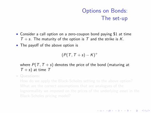
• Consider a call option on a zero-coupon bond paying $1 at timeT + s. The maturity of the option is T and the strike is K .
• The payoff of the above option is
(P(T ,T + s)− K )+
where P(T ,T + s) denotes the price of the bond (maturing atT + s) at time T
• Questions:How do we apply the Black-Scholes setting to the above option?What are the correct assumptions that are analogues of thelognormallity we imposed on the prices of the underlying asset in theBlack-Scholes pricing model?
Options on Bonds:The set-up
• Consider a call option on a zero-coupon bond paying $1 at timeT + s. The maturity of the option is T and the strike is K .
• The payoff of the above option is
(P(T ,T + s)− K )+
where P(T ,T + s) denotes the price of the bond (maturing atT + s) at time T
• Questions:How do we apply the Black-Scholes setting to the above option?What are the correct assumptions that are analogues of thelognormallity we imposed on the prices of the underlying asset in theBlack-Scholes pricing model?

Exchange Options:The definition and set-up
• It turns out that the convenient tool for solving the above problem isto recast the set-up in terms of a particular family of exoticoptions, namely, exchange options.
• An exchange option pays off only if the underlying asset outperformssome other asset (benchmark). Hence, these options are also calledout-performance options
• Consider an exchange call option maturing T periods from nowwhich allows its holder to obtain 1 unit of risky asset #1 in returnfor one unit of risky asset #2.
• St . . . the price of the risky asset #1 at time t
• Kt . . . the price of the risky asset #1 at time t
• δS . . . the dividend yield of the risky asset #1
• δK . . . the dividend yield of the risky asset #2
• σS , σK . . . the volatilities of the risky assets #1 and #2, respectively
• ρ . . . the correlation between the two assets

Exchange Options:The pricing formula
•
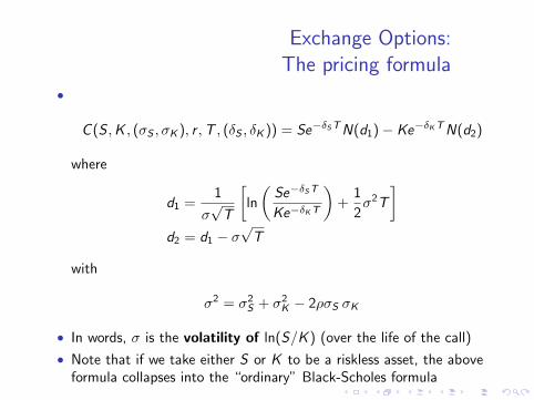
C (S ,K , (σS , σK ), r ,T , (δS , δK )) = Se−δSTN(d1)− Ke−δK TN(d2)
where
d1 =1
σ√
T
[ln
(Se−δST
Ke−δK T
)+
1
2σ2T
]d2 = d1 − σ
√T
with
σ2 = σ2S + σ2
K − 2ρσS σK
• In words, σ is the volatility of ln(S/K ) (over the life of the call)
• Note that if we take either S or K to be a riskless asset, the aboveformula collapses into the “ordinary” Black-Scholes formula

Exchange Options:The pricing formula
•
C (S ,K , (σS , σK ), r ,T , (δS , δK )) = Se−δSTN(d1)− Ke−δK TN(d2)
where
d1 =1
σ√
T
[ln
(Se−δST
Ke−δK T
)+
1
2σ2T
]d2 = d1 − σ
√T
with
σ2 = σ2S + σ2
K − 2ρσS σK
• In words, σ is the volatility of ln(S/K ) (over the life of the call)
• Note that if we take either S or K to be a riskless asset, the aboveformula collapses into the “ordinary” Black-Scholes formula
Exchange Options:Application to options on bonds
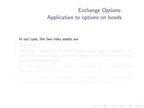
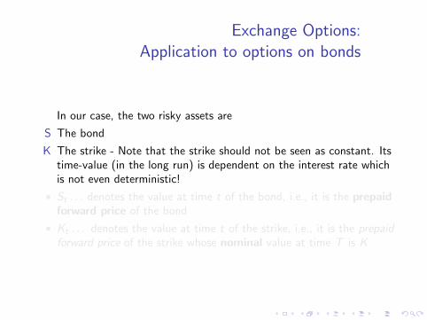
In our case, the two risky assets are
S The bond
K The strike - Note that the strike should not be seen as constant. Itstime-value (in the long run) is dependent on the interest rate whichis not even deterministic!
• St . . . denotes the value at time t of the bond, i.e., it is the prepaidforward price of the bond
• Kt . . . denotes the value at time t of the strike, i.e., it is the prepaidforward price of the strike whose nominal value at time T is K

Exchange Options:Application to options on bonds
In our case, the two risky assets are
S The bond
K The strike - Note that the strike should not be seen as constant. Itstime-value (in the long run) is dependent on the interest rate whichis not even deterministic!
• St . . . denotes the value at time t of the bond, i.e., it is the prepaidforward price of the bond
• Kt . . . denotes the value at time t of the strike, i.e., it is the prepaidforward price of the strike whose nominal value at time T is K

Forward Contracts Revisited
• Recall that a forward contract is an agreement to pay a specifieddelivery price K at a delivery date T in exchange for an asset
• Let the asset’s price at time t be denoted by St .
• Then, we denote the T -forward price of this asset at time t byFt,T [S ].
• It is defined as the value of the delivery price K which makes theforward contract have the no-arbitrage price at time t equal to zero.

Forward Contracts:Connection with bond-prices
• Theorem: Assume that zero-coupon bonds of all maturities are/canbe traded. Then,
Ft,T [S ] =St
P(t,T ), for 0 ≤ t ≤ T
• The argument:
Suppose that at time t you:
1. Sell the above forward contract - this is not a “real sale” as noincome can be generated in doing so (by definition)
2. Also, you short St
P(t,T ) zero-coupon bonds - doing so you get the
income of St
3. With the above produced income St , you by one share of the asset S

Forward Contracts:Connection with bond-prices (cont’d)
You do nothing until time T
Then, at time T you:
1. Deliver the one share of asset S that you own
2. Get the delivery price K in return
3. Cover the short bond position - recall that the bonds we shorted allhad maturity T at which time they are worth exactly $1, i.e., theamount of the payment they produce at maturity
• The net-effect at time T is that you have K − St
B(t,T ) - this value
must be equal to zero, or else there is arbitrage

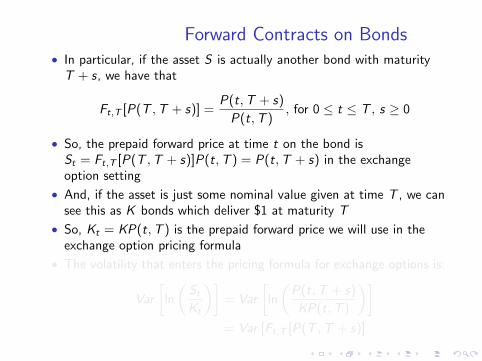
Forward Contracts on Bonds• In particular, if the asset S is actually another bond with maturity
T + s, we have that
Ft,T [P(T ,T + s)] =P(t,T + s)
P(t,T ), for 0 ≤ t ≤ T , s ≥ 0
• So, the prepaid forward price at time t on the bond isSt = Ft,T [P(T ,T + s)]P(t,T ) = P(t,T + s) in the exchangeoption setting
• And, if the asset is just some nominal value given at time T , we cansee this as K bonds which deliver $1 at maturity T
• So, Kt = KP(t,T ) is the prepaid forward price we will use in theexchange option pricing formula
• The volatility that enters the pricing formula for exchange options is:
Var
[ln
(St
Kt
)]= Var
[ln
(P(t,T + s)
KP(t,T )
)]= Var [Ft,T [P(T ,T + s)]

Black formula
• If we assume that the bond forward price process{Ft,T [P(T ,T + s)]}t agrees with the Black-Scholes assumptionsand that its constant volatility is σ, we obtain the Black formula fora bond option:
C [F ,P(0,T ), σ, T ] = P(0,T )[FN(d1)− KN(d2)]
where
d1 =1
σ√
T
[ln(F/K ) +
1
2σ2T
]d2 = d1 − σ
√T
with F = F0,T [P(T ,T + s)]
Forward (Implied) Interest Rate
• We are now at time 0.Assume that you would like to earn at the interest rate in the periodbetween time T and time T + s. Denote this forward interest rateby R0(T ,T + s).
• The unit investment in the interest rate at time T until time T + sshould be consistent (in the sense of no-arbitrage) with the strategythat includes a zero-coupon bond maturing at time T and anotherwith maturity at time T + s, i.e., we should have
1 + R0(T ,T + s) =P(0,T )
P(0,T + s)

Forward Rate Agreements
• Consider a borrower (or, analogously, a lender) who wants to hedgeagainst increases in the cost of borrowing a certain amount ofmoney at a future date (that is, in the interest rate)
• Forward rate agreements (FRAs) are over-the-counter contracts thatguarantee a borrowing or lending rate on a given principal amount
• FRAs are, thus, a type of forward contracts based on the interestrate:If the reference (“real”) interest rate is above the rate agreed uponin the FRA, then the borrower gets paid.If the reference (“real”) interest rate is below the rate agreed uponin the FRA, then the borrower pays.

Forward Rate Agreements:Settlement time
• FRAs can be settled at maturity (in arrears), i.e., at the time theloan is repaid or at the initiation of the borrowing or lendingtransaction, i.e., at the time the loan is taken
• Let r denote the reference interest rate for the prescribed loan period
• If in arrears, then the payment is
(r − rFRA)× notional principal
• If at the initiation, then the payment is
1
1 + r× (r − rFRA)× notional principal
Forward Rate Agreements:Hedging
• One way to hedge the risk coming from the changes in the interestrate is, then, a simple FRA
• If the settlement is conducted in arrears, the payoff at time T + s is
spot s-period rate− forward rate = RT (T ,T + s)− R0(T ,T + s)
• Alternatively, one (in this case a borrower) might buy a call optionon the FRA - this should be a better strategy as there is nodownfall in dropping interest rates

Forward Rate Agreements:Caplets
• Options on the FRA are called caplets
• This option, at time T + s pays
(RT (T ,T + s)− KR)+
where KR denotes the strike
• If settled at time T , then the above type of option has payoff
1
1 + RT (T ,T + s)(RT (T ,T + s)− KR)+
due to “discounting”
• The above is the value (price) of the contract at time T

Forward Rate Agreements:Pricing caplets through the Black formula
• Using simple algebra, we can transform the above payoff into
(1 + KR)
(1
1 + KR− 1
1 + RT (T ,T + s)
)+
• Recalling the consistency equation
1 + R0(T ,T + s) =P(0,T )
P(0,T + s)
we see that the value 11+RT (T ,T+s) is the value at time t of a
zero-coupon bond paying $1 at time T + s
• Setting the value 11+KR
as the new strike, we see that we can use theBlack formula to price the above described caplet

Forward Rate Agreements:Caps
• An interest rate cap is a collection of caplets
• Suppose a borrower has a floating rate loan with interest paymentsat times ti , i = 1, ..., n. A cap would make the series of payments attimes ti+1 given by
(Rti (ti , ti+1)− KR)+

Forward Rate Agreements:Caps
• An interest rate cap is a collection of caplets
• Suppose a borrower has a floating rate loan with interest paymentsat times ti , i = 1, ..., n. A cap would make the series of payments attimes ti+1 given by
(Rti (ti , ti+1)− KR)+