bipole iii transmission project - manitoba hydro · pdf filebipole iii transmission project...
TRANSCRIPT
Bipole III Transmission Project
Electromagnetic Fields (EMF)Technical Report
Exponent Inc.November 2011
Health Sciences Practice
Manitoba Hydro Bipole III
Environmental and Health Assessment of the Electrical Environment
Direct Current Electric and Magnetic Fields and Corona Phenomena

0704235.001 D0T0 1111 WHB6
Manitoba Hydro Bipole III
Environmental and Health Assessment of the Electrical Environment
Direct Current Electric and Magnetic Fields and Corona Phenomena Prepared for Manitoba Hydro Prepared by Exponent 17000 Science Drive, Suite 200 Bowie, MD 20715 November 24, 2011 © Exponent, Inc.

November 24, 2011
0704235.001 D0T0 0811 WHB5 ii
Contents
Page
List of Figures ii
List of Tables iii
Acronyms and Abbreviations iv
Unit Definitions and Conversions vi
Notice vii
Executive Summary viii
Introduction 1
Methodology 6
Study areas 6
Issue identification 6
Exposure assessment 7
Criteria for impact assessment 7
The Nature of the Electrical Environment 8
Static electric and magnetic fields 9 Static electric fields 9 Static magnetic fields 10
Corona phenomena 12 Space charge 13 Ion current density 17 Air quality 17
Audible noise 18
Radio noise 20
Scientific Reviews and Guidelines 22
American Conference of Governmental Industrial Hygienists 24
Health Canada 24

November 24, 2011
0704235.001 D0T0 0811 WHB5 iii
International Agency for Research on Cancer 25
International Commission on Non-Ionizing Radiation Protection 25
International Committee on Electromagnetic Safety 25
Minnesota Environmental Quality Board 26
National Radiological Protection Board 27
U.S. Food and Drug Administration 28
World Health Organization 29
Electrical Environment of Bipole III – Static Fields 31
DC electric field 31
DC magnetic field 33
Electrical Environment of Bipole III – Space Charge 34
Electrical Environment of Bipole III – Audible Noise and Radio Noise 38
Additional corona phenomena 38 Audible noise 38 Radio noise 38 Visible light 38
Interference with electronic devices 39 Global Positioning System receivers 39 Mining surveying equipment 41 Electronic medical devices 42
Dairy Cattle, Wild Animals, and Plants 48
Dairy cattle and DC transmission lines 48
Plants 49
Wild animals 50
Ancillary DC Facilities 53
Converter Station 53
Ground electrode/feeder line 53
References 55

November 24, 2011
0704235.001 D0T0 0811 WHB5 iv
Appendix 1 - Modeling of the Electrical Environment for the Proposed DC Components of the Bipole III Project
Appendix 2 - Space charge and research on the respiratory system, mood, and behavior

November 24, 2011
0704235.001 D0T0 0811 WHB5 ii
List of Figures
Page
Figure 1. Bipole III preferred route 3
Figure 2. Map of the Earth’s geomagnetic field (NOAA/NGDC, 2010) 11
Figure 3. Relationship of corona-related phenomena 13
Figure 4. Fraction of all aerosols (0.65 µm – 1.00 µm) carrying charges in outdoor settings in the vicinity of Winnipeg, Manitoba and Chicago, Illinois. 17
Figure 5. Timeline of major scientific organizations reviewing research related to static magnetic and electric fields since 2000 23
Figure 6. Charged aerosol fraction (%) with respect to distance from the centerline of the ±450-kV and ±500-kV transmission lines in Manitoba 36
Figure 7. Charging model for person standing under the Bipole III line 44
Figure 8. DC resistance of persons through shoes, standing on various surfaces 47

November 24, 2011
0704235.001 D0T0 0811 WHB5 iii
List of Tables
Page
Table 1. Typical static electric field levels from common natural and man-made sources 10
Table 2. Typical static magnetic field levels from common natural and man-made sources 12
Table 3. Typical concentrations of air ions 15
Table 4. Aerosol concentrations and rough estimates of singly charged aerosols 0.16-0.24 µm (% of total charged) in various locations 16
Table 5. Range of levels of airborne aerosols (0.65 - 1 µm) carrying electrical charges (percent) 16
Table 6. Examples of audible noise levels 20
Table 7. Comparison of screening guidelines for public exposure to DC and 60-Hz AC magnetic fields 26
Table 8. Comparison of air ion levels from the proposed project to other sources 35

November 24, 2011
0704235.001 D0T0 0811 WHB5 iv
Acronyms and Abbreviations
µA Microampere µm Micrometre µT Microtesla A Ampere AC Alternating current ACGIH American Conference of Governmental Industrial Hygienists AGNIR Advisory Group on Non-Ionising Radiation AM Amplitude modulated AN Audible noise cm Centimetre dB Decibels dB-A Decibels on the A-weighted scale DC Direct current DGPS Differential global positioning system ESD Electrostatic discharge FDA US Food and Drug Administration Fe3O4 Magnetite FM Frequency modulated G Gauss GHz Gigahertz GΩ Giga-ohm GNSS Global navigation satellite system GPS Global positioning system HEM Helicopter electromagnetic Hz Hertz IARC International Agency for Research on Cancer ICES International Committee on Electromagnetic Safety ICNIRP International Commission for Non-Ionizing Radiation Protection IEC International Electrotechnical Commission Ions/cm3 Ions per square centimetre kHz Kilohertz km Kilometre kV Kilovolt kV/cm Kilovolt per centimetre kV/m Kilovolt per metre

November 24, 2011
0704235.001 D0T0 0811 WHB5 v
m Metre MEQB Minnesota Environmental Quality Board mG Milligauss MHz Megahertz MHRF Ministry of Health of the Russian Federation mm Millimetre mT Millitesla MRI Magnetic resonance imaging MSAT Mobile satellite MW Megawatt mV Millivolt nA/m2 Nanoamperes per square metre NDGPS Nationwide differential global positioning system nm Nanometre
NRPB National Radiation Protection Board of Great Britain nT Nanotesla O3 Ozone ppb Parts per billion Rad/s Radians per second RF Radiofrequency RMS Root mean square RN Radio noise ROW Right-of-way RTK Real-time kinetic T Tesla SCENIHR Scientific Committee for Emerging and Newly Identified Health Risks SPL Sound pressure level UHF Ultra high frequency VDU Video display units VHF Very high frequency V/m Volts per metre WHO World Health Organization

November 24, 2011
0704235.001 D0T0 0811 WHB5 vi
Unit Definitions and Conversions
Multiple units are often used to quantify levels of the same electrical phenomenon. The following tables are provided to assist the reader in understanding the relationship of different units for common electrical phenomenon (current, voltage, electric fields, and magnetic fields). The relationship between magnetic flux density (B), expressed in Tesla (T) and magnetic field (H), expressed in Amperes/metre (A/m), , is given by B = µH where µ is the magnetic permeability of the medium. The permeability of biological materials and water is similar to that of air µ0 (1.257 x 10⁻⁶ Henries/metre) so that 1 T = 7.96 x 10⁵ A/m.
Current Unit Abbreviation Conversion to A
Ampere A Milliampere mA 0.001 A Microampere µA 0.000001 A Nanoampere nA 0.000000001 A
Voltage Unit Abbreviation Conversion to V
Volt V Kilovolt kV 1,000 V Millivolt mV 0.001 V Microvolt µV 0.000001 V
Electric Field Unit Abbreviation Conversion to V/m
Volt/metre V/m Kilovolt/metre kV/m 1,000 V/m
Magnetic Flux Density (i.e., Magnetic Field) Unit Abbreviation Conversion
Gauss G Milligauss mG 0.001 G = 0.1 µT Tesla T 1 Weber/m2 Millitesla mT 0.001 T = 10 G Microtesla µT 0.000001T = 10 mG Nanotesla nT 0.000000001 T = 0.01 mG

November 24, 2011
0704235.001 D0T0 0811 WHB5 vii
Notice
At the request of Manitoba Hydro, Exponent conducted specific modeling and evaluations of
components of the electrical environment of the Bipole III project. This report summarizes
work performed to date and presents the findings resulting from that work. In the analysis, we
have relied on geometry, material data, usage conditions, specifications, regulatory status, and
various other types of information provided by the client. We cannot verify the correctness of
this input data, and rely on the client for their accuracy. Although Exponent has exercised usual
and customary care in the conduct of this analysis, the responsibility for the design and
operation of the project remains fully with the client.
The findings presented herein are made to a reasonable degree of engineering and scientific
certainty. Exponent reserves the right to supplement this report and to expand or modify
opinions based on review of additional material as it becomes available, through any additional
work, or review of additional work performed by others.
The scope of services performed during this investigation may not adequately address the needs
of other users of this report, and any re-use of this report or its findings, conclusions, or
recommendations presented herein are at the sole risk of the user. The opinions and comments
formulated during this assessment are based on observations and information available at the
time of the investigation. No guarantee or warranty as to future life or performance of any
reviewed condition is expressed or implied.

November 24, 2011
0704235.001 D0T0 0811 WHB5 viii
Executive Summary
The components of the Bipole III project―transmission lines, converter stations, and ground
electrodes―are all sources of direct current (DC) electric and magnetic fields and related corona
phenomena, including space charge (air ions and charged aerosols), audible noise (AN), and
radio noise (RN).
The purpose of this assessment is to describe the exposures associated with these components of
the Bipole III electrical environment and to determine if and how exposure may affect humans,
domestic animals, wildlife, and plants in the project area.
DC electric and magnetic fields (also called static fields because of their unvarying nature in
time) and space charge are everywhere in the natural environment. The most prevalent static
magnetic field is produced by the Earth as a result of constant flow of current deep within the
Earth’s core. This is called the Earth’s geomagnetic field and it is this field that is used for
compass navigation. Static electric fields are produced by many natural phenomena including
that produced by charges accumulated on clothing after walking across a carpet. Other common
natural sources of DC electric fields include weather phenomena such as storm clouds, blowing
snow, and swirling dust clouds.
Electrical charges in the air, referred to as space charge, are formed by many common natural
sources: by the Earth and its atmosphere, energy released by evaporation (i.e., the break-up of
water droplets), friction from blowing snow and swirling dust, open flames and other
combustion processes, and various meteorological events. These charges may provide the basis
for a clustering of gas molecules (air ions) or may become attached to passing solid or liquid
particles (charged aerosols). Collectively, air ions charged aerosols are referred to as space
charge.
The changes to the background electrical environment expected from the operation of Bipole III
were modeled and the resulting levels compared to relevant standards and guidelines. In
addition, numerous reviews of the scientific literature by scientific and regulatory agencies on
static electric and magnetic fields and related phenomena were consulted including those by the

November 24, 2011
0704235.001 D0T0 0811 WHB5 ix
American Conference of Governmental Industrial Hygienists (ACGIH), Health Canada, the
International Agency for Research on Cancer (IARC), the International Commission on Non-
ionizing Radiation Protection (ICNIRP), the International Committee on Electromagnetic Safety
(ICES), the Minnesota Environmental Quality Board (MEQB), the National Radiological
Protection Board (NRPB), the U.S. Food and Drug Administration (FDA), and the World
Health Organization (WHO).
DC electric fields from the Bipole III line are not capable of coupling effectively to conductive
objects and so the currents intercepted by a person under a DC transmission line are on the order
of a few microamperes (µA), which is below the threshold for detection of DC currents. Even
for large vehicles parked underneath a DC transmission line or long parallel fences, the charge
collected is limited by leakage current to the ground so the possibility of perception is limited;
under experimental ‘worst case’ conditions, the only noticeable effect of touching a large, well
grounded vehicle would be a microshock, weaker than what a person might experience after
crossing a carpet.
The static magnetic field will be increased above background levels on portions of the right-of-
way (ROW) and decreased below background levels on other portions of the ROW. Outside the
ROW, there will be an insignificant change in the background geomagnetic field.
When the strength of the electric field at points on the conductor surface exceeds a threshold or
onset level, a small amount of energy is released by a partial electrical discharge (called corona)
that can lead to air ions, charged aerosols, audible noise (AN), and radio noise (RN). There are
no guidelines for exposures to air ions and charged aerosols, but the modeled levels outside the
ROW are expected to be similar to those of other DC transmission lines in North America and
within the range of levels produced by other ambient sources. The levels of AN will be well
below provincial standards and RN will be well below the national Canadian standard.
The proliferation of electronic devices for personal, recreational, commercial, and medical uses
had prompted questions as to whether the Bipole III transmission line will affect their
performance. The Global Positioning System (GPS) is a space-based navigation system that
relies on 24 orbiting satellites circling Earth to establish the position of a GPS receiver on the
Earth. The receiver uses the radiofrequency (RF) signals sent from three or more of these

November 24, 2011
0704235.001 D0T0 0811 WHB5 x
satellites to determine its exact location. Naturally-occurring sources of RF (e.g., geomagnetic
storms) and man-made sources of RF (e.g., TV station transmitters) are sometimes reported to
interfere with GPS signals because these sources produce RF in the same frequency range as the
GPS. Since GPS signals are of far higher frequency than the RN produced by a DC
transmission line, however, it is very unlikely that a DC transmission line will interfere with
GPS functioning. In addition, tests of a variety of GPS receivers performed for Manitoba Hydro
under the existing Bipole I and II transmission lines were unable to detect any impairment in
GPS performance due to RN.
The northern portion of the project study area includes mining leases within the Thompson
Nickel Belt and sensitive electronic methods are used in surveys to detect conductive ore
deposits. Whether the fields from the proposed Bipole III transmission line will interfere with
mining exploration survey methods depends on the distance to the line, the type of measurement
equipment used for the explorations, and post-processing corrections of the acquired data.
Mitigation methods include avoiding or minimizing potential interference with mining
exploration by encouraging mining companies to conduct surveys before the construction of
Bipole III in 2017, applying filters during post-survey processing to remove extraneous
magnetic ‘noise,’ using survey methods less susceptible to interference, and shifting the route of
the line further from mining claims.
The magnetic field from a DC line is too weak to affect cardiac pacemakers. Since the
background level of the static magnetic field in Manitoba is approximately 580 milligauss (mG)
(58 microtesla [µT]) and the maximum increase from Bipole III is estimated to be less than
twice this background level, the exposures to a person with an implanted pacemaker even under
the transmission line will be far below the recommended exposure limit of 0.5 millitesla (mT)
(5,000 mG) (ACGIH, 2009). Similarly, the static electric field from a DC line would not be
expected to be a source of interference to a pacemaker or cause human-body potentials to
exceed the International Electrotechnical Commission’s (IEC) immunity-test levels for a
cochlear implant.
Converter stations (where alternating current [AC] power is converted to DC power and vice
versa) and the ground electrodes at each end of the line are necessary for operation of the Bipole

November 24, 2011
0704235.001 D0T0 0811 WHB5 xi
III line. The levels of DC electric fields and magnetic fields from these sources are low outside
the facility property. During some modes of monopolar operation prompted by maintenance or
equipment breakdown, the full load current may be carried on a feeder line to the ground
electrode to complete the circuit via a conductive path deep in the Earth. The magnetic field at
points under the electrode line and at line termination would be higher than on the Bipole III
ROW but still very low and well below international standards. Based on evaluations
performed by Teshmont of step potentials and other considerations, temporary monopolar
operation would not pose risks to the safety of persons and animals. Confirmation of these
results under a wider range of assumptions and the calculation of touch potential is
recommended. While incomplete filtering of harmonic currents at the converter station in
monopolar operation might cause interference to nearby susceptible telephone communications,
this possibility can be reduced in the design stage, or mitigated if further reductions are required
later.
In summary, the electrical environment is expected to conform to exposure limits recommended
by provincial, national, and international agencies. A comparison between Bipole III and six
other DC transmission lines in North America shows that the median peak levels of DC electric
fields and small air ions of Bipole III are lower than the levels of five other DC transmission
lines. The field levels of the proposed line were not found to pose any likely effect on electronic
devices nor were adverse effects of the ground electrode/feeder line identified that could not be
mitigated.
It is noted that this Executive Summary cannot summarize all of Exponent’s technical
evaluation, analysis, conclusions, and recommendations. Hence, the main part of this report and
its Appendices are at all times the controlling document.

November 24, 2011
0704235.001 D0T0 1111 WHB6
1
Introduction
Manitoba Hydro has proposed to construct a new ±500-kilovolt (kV) direct current (DC)
transmission line (Bipole III). Bipole III will link the existing northern power generating
facilities on the Nelson River with the existing alternating current (AC) system that delivers
electricity to homes, offices, factories, and other facilities in southern Manitoba. Manitoba
currently has two DC transmission lines, Bipole I and Bipole II on the same corridor, which carry
power generated on the Nelson River to the greater Winnipeg area. The addition of Bipole III to
a different corridor will improve the reliability of the province’s electricity supply.
DC transmission was selected for this particular project because it is more effective in
transmitting electricity over long distances than AC transmission. Foremost, DC transmission
has less power loss because of the direct nature of current flow; AC electricity flows more at the
surface of the conductors, which results in higher resistance and more line losses. DC
transmission also requires less extensive facilities—smaller towers and fewer insulators and
conductors—than AC transmission. The major issue that can offset these advantages is the cost
and complexity of converting between AC and DC power. For this reason, DC transmission
lines are most practical in the circumstance where a large amount of power is being transmitted
over a long distance, without the need to tap power off along the way (e.g., only two converter
stations needed).
The preferred route is approximately 1,384 kilometres (km) (Figure 1). The route will originate
near Gillam (Keewatinoow); it will continue west and south towards The Pas; it will proceed
south to the west of Lake Winnipegosis and Lake Manitoba; and it will pass south of Portage la
Prairie and Winnipeg. Finally, the route will terminate at the Riel Converter Station in the rural
municipality of Springfield.
Converter stations are also required to convert the AC power from the generators to DC power
and then back to AC power for distribution. The project consists of building two, new converter
stations―one northeast of Gillam (Keewatinoow) in northern Manitoba and the other east of
Winnipeg at the Riel Station site. In addition, Manitoba Hydro plans to install two ground
electrodes, one connected to each converter station. Finally, 230-kV AC transmission line
interconnections will tie the new Keewatinoow converter station into the existing AC

November 24, 2011
0704235.001 D0T0 1111 WHB6
2
transmission system and generating stations in North Manitoba. The electrical environment and
assessment of these 230-kV AC lines are the subject of another Exponent report “Environmental
and Health Assessment of the Electrical Environment—Alternating Current Electric and
Magnetic Fields and Corona Phenomena.”
The conductors of the proposed DC transmission line will be strung on steel tower structures on a
66 metre (m) wide right-of-way (ROW). The towers will be spaced approximately 480 m apart,
resulting in two to three towers per km (i.e., three to four towers per mile). Two types of towers
will be used, depending on the area’s terrain: self-supporting lattice towers will be used in
agricultural areas to minimize the impact on agricultural operations and guyed towers will be
used in forested areas and other suitable areas.

November 24, 2011
0704235.001 D0T0 1111 WHB6
3
Figure 1. Bipole III preferred route
The components of the Bipole III project―transmission lines, converter stations, and
substations―are all sources of electric and magnetic fields and related corona phenomena
including space charge (small air ions and charged aerosols), audible noise (AN), and radio noise
(RN).

November 24, 2011
0704235.001 D0T0 1111 WHB6
4
During the consultation process comments from the public raised questions about electric and
magnetic fields in relation to general health, animals, research, electronics and machinery, and
medical devices, which resulted in electric fields, magnetic fields, and related phenomena being
the fourth most common topic.1 The purpose of this assessment is to determine if and how the
operation of these project components may affect humans, domestic animals, wildlife, and plants
in the project area, and in so doing address the issues raised by these comments. Specific criteria
are used to evaluate the possible impact of the electrical environment, as described in the
Methodology section below. Other sections of this report include the following:
• The Nature of the Electrical Environment summarizes the basic properties of the study
areas for this report (i.e., DC electric and magnetic fields and corona phenomena),
including sources and typical exposure levels.
• Scientific Reviews and Guidelines for Direct Current Electric and Magnetic Fields
summarizes the conclusions of reviews published by scientific agencies related to DC
fields and corona ion phenomena. These reviews address the health and safety of humans
(a key identified issue for this project) and provide recommended standards and
guidelines for levels of DC electric and magnetic fields, AN, and RN. These guidelines
provide the criteria used for assessing the impact of the Bipole III project.
• Electrical Environment of Bipole III – Static Fields summarizes the calculated levels
of static electric and magnetic fields from the proposed Bipole III line, compares them to
relevant guidelines, and provides an assessment of the likelihood and nature of any
expected impacts.
• Electrical Environment of Bipole III – Space Charge summarizes the calculated levels
of air ions from the proposed Bipole III line, compares them to other DC lines in North
America, and assesses the likelihood and nature of expected impacts based on a review of
health-related research and measurements of charged aerosols around the existing Bipole
I and II lines in Manitoba.
1 Bipole III Newsletter Round Four – Preliminary Preferred Route
http://www.hydro.mb.ca/projects/bipoleIII/bipoleIII_newsletter4.pdf

November 24, 2011
0704235.001 D0T0 1111 WHB6
5
• Electrical Environment of Bipole III – Audible Noise and Radio Noise summarizes
the calculated levels of AN and RN from the proposed Bipole III line, compares these
levels to relevant guidelines, and provides an assessment of the likelihood and nature of
any expected impacts. This section also summarizes the potential for interference to
mining surveys, Global Positioning System (GPS) equipment, and electronic medical
devices, issues that were raised during stakeholder consultations on this project.
• Research on Dairy Cattle, Wild Animals, and Plants reviews the cumulative research
related to DC electric and magnetic fields and dairy cattle, wild animals, crops, and
natural flora, topics also raised during stakeholder consultations on this project.

November 24, 2011
0704235.001 D0T0 1111 WHB6
6
Methodology
The procedure for conducting this assessment involves the delineation of study areas, the
identification of important issues, and the determination of valid assessment evaluation criteria.
Study areas
While the Bipole III transmission line project encompasses a large geographic area, the potential
for interactions of electrical components with the surrounding environment is much more limited.
This report describes the nature of these electrical components to provide the reader with an
understanding of their basic characteristics and mechanisms of interaction. These phenomena
include the following features of the electrical environment surrounding a DC transmission line:
(1) the DC electric field, (2) the DC magnetic field, and (3) various corona phenomena, including
AN, RN, and space charge.
These study areas are described in detail in the section The Nature of the Electrical
Environment below.
Issue identification
Technical issues were identified using knowledge of issues addressed during the previous siting
process of existing DC transmission lines and from stakeholder input for this specific project.
Major issues that were judged to warrant investigation pertaining to the study areas include the
effect of these phenomena on the health and safety of humans, animals, and plants. Aspects of
the electrical environment that were addressed by measurements around the Bipole I and Bipole
II DC transmission lines in Manitoba (Maruvada et al., 1982) continued to warrant discussion in
this assessment. Other technical issues for further study and assessment were identified by
Exponent scientists and engineers and from stakeholder input at public open house meetings and
submissions to Manitoba Hydro. These include an assessment of charged aerosols, the effects of
DC electric and magnetic fields on wildlife, and potential interference to electronic devices such
as GPS receivers used in agriculture, devices used for mining surveys, and electronic medical
devices.

November 24, 2011
0704235.001 D0T0 1111 WHB6
7
Exposure assessment
To characterize how the Bipole III project might affect the background electrical environment,
the DC transmission lines and other DC components (including the converter stations and ground
electrodes) were modeled to describe the spatial distribution of fields and currents and site-
specific land uses (Appendix 1). The basis for modeling the charging of aerosols by DC lines is
not well developed so a field study was also undertaken to measure the levels of charged aerosols
upwind and downwind of the existing Bipole I/II transmission lines in the province.
Criteria for impact assessment
Criteria by which to distinguish potentially significant effects of the Bipole III project on health
and the environment were identified by reference to published scientific reviews by national and
international agencies, specifically the guidelines and standards established by these agencies.
These guidelines and standards serve as criteria for the assessment of DC electric fields, DC
magnetic fields, AN, and RN.
No such established criterion for the assessment of air ions was identified. Therefore, to provide
a solid basis for conclusions on this topic a weight-of-evidence review of individual research
studies was performed using the standard scientific methods recommended and followed by
health and scientific agencies. The review of this research, including supplemental tables
summarizing each study, is included as Appendix 2.

November 24, 2011
0704235.001 D0T0 1111 WHB6
8
The Nature of the Electrical Environment
A DC transmission line has two conductors or conductor bundles, called “poles.” The voltages
on the poles are usually of opposite polarity―one positive (+) and one negative (-). The
operating voltage of a DC transmission line is usually expressed in terms of the voltage on both
poles, i.e., Bipole III is described as a ±500-kV transmission line.
The electrical environment surrounding a DC transmission line is primarily influenced by three
primary electrical phenomena (a DC electric field, a DC magnetic field, and corona). Other
phenomena including AN, RN, ion current density and ozone are secondary to corona discharge.
• The magnetic fields from a DC transmission line arise from the current flowing on the
conductors and are commonly expressed as magnetic flux density in units of gauss (G) or
milligauss (mG).2
• The electric fields from a DC transmission line arise from the voltage on the lines and are
measured in units of kilovolts per metre (kV/m). Both DC magnetic and electric fields
are identified as “direct” because they do not oscillate over time, or change very slowly
(i.e., 0 Hertz [Hz]); for this reason, they also are most often referred to as static fields.3
• Corona discharge refers to the partial electric discharge (energy loss) that occurs when the
electric field at a point on the conductor is strong enough to remove electrons from air
molecules (ionize the air molecules). Corona results in electrical charges being
transferred on air molecules referred to as small air ions. These air ions exist only for a
matter of seconds before they are neutralized. A fraction of the charge from these air ions
is transferred to ambient aerosols, which are then described as charged aerosols.
The general aspects of these electrical factors are fully discussed in this section.
2 The magnetic flux density (B) vector is most often used to express the intensity of a magnetic field. In Europe
and in technical publications, magnetic flux density is presented in units of tesla (T), the expression used by the International System of Units (Le Système International d'Unités), where 1 T =10,000 G and 1 mG = 0.1 µT. In North America, magnetic flux density is more often expressed in G or mG. See the Unit Definitions and Conversion Charts on page iv.
3 In comparison, AC electric and magnetic fields from electricity transmitted in North America vary at a frequency of 60 times per second (60 Hz); electricity in other areas of the world may be transmitted at 50 Hz.

November 24, 2011
0704235.001 D0T0 1111 WHB6
9
Static electric and magnetic fields
Electric and magnetic fields exert forces on electric charges and so are associated with anything
that generates, transmits, or uses electricity, both in the AC and DC form. While both AC and
DC electricity are sources of electric and magnetic fields, there are substantial differences in the
characteristics of these phenomena and, as a result, their potential interactions with people and
the environment. These differences stem from the basic fact that current does not alternate when
transmitted as DC, while it alternates with a regular frequency when transmitted as AC. As a
result of the static nature of DC, there is no significant induction of voltage or current in
conductive materials (such as people) with DC fields. Currents are only induced when there is
motion by an object or subject in a very high intensity static magnetic field.
Another major difference between AC and DC fields is that DC fields are commonly encountered
from many natural sources, as described below. DC fields have been present throughout the
evolution of life on Earth and, while this does not preclude any adverse effects, it indicates a
natural relationship.
Static electric fields
Static electric fields are produced by a number of man-made sources, as well as many natural
phenomena. Electric charges in the atmosphere, for example, produce a static electric field with
an intensity of about 0.15 kV/m (Chalmers, 1967; Barnes, 1986). Everyone has experienced
static electricity as the electric shock felt after walking across a carpet and the ‘static cling’ that
develops on a comb, brush, or on clothing. Other common natural sources of DC electric fields
include weather phenomena such as storm clouds, blowing snow, and swirling dust clouds. In
addition to transmission lines, man-made sources of electric fields include electrified railway
systems and, although less common today, cathode ray tubes (CRT) in older computer and
television picture screens.
A person’s static electric field exposure depends on the frequency with which he or she
encounters these sources, as well as the distance from these sources. Static electric fields
decrease rapidly with distance from their source. Furthermore, common objects (such as trees,
fences, and buildings) block static electric fields, such that outside sources cannot be measured
indoors.

November 24, 2011
0704235.001 D0T0 1111 WHB6
10
Table 1 describes the typical static electric field levels associated with common sources. This
table illustrates that 1) we are surrounded by natural sources of DC electric fields; and 2) static
electric field levels associated with DC transmission lines are in the range of common sources.
Table 1. Typical static electric field levels from common natural and man-made sources
Source Electric Field Level (kV/m)
Man-made Sources
TV and CRT computer screens (at 30 centimetres) 10–20
Under a ±500-kV transmission line 20-30
Natural Sources
Distant storm front 10-20
Storm cloud over a lake 40
Friction from walking across a carpet Up to 100
Surface charge on the body from static cling Up to 500
Source: Johnson, 1985; Barnes, 1986
Static magnetic fields
Just like static electric fields, static magnetic fields are produced by numerous man-made and
natural sources. The most prevalent static magnetic field is that produced by the Earth as a result
of constant flow of current deep within the Earth’s outer core. This is called the Earth’s
geomagnetic field and it is this field that is used for compass navigation. The geomagnetic field
ranges in intensity from 300-700 mG, varying at different latitudes. It is highest at the magnetic
poles and lowest at the equator. The strength of this field in Manitoba is about 580 mG (NGDC,
2010). Depending on the orientation of a DC transmission line with respect to the magnetic field
of the Earth, a DC transmission line can either add to or subtract from the strength of the Earth’s
geomagnetic field.

November 24, 2011
0704235.001 D0T0 1111 WHB6
11
Figure 2. Map of the Earth’s geomagnetic field (NOAA/NGDC, 2010)
DC magnetic fields are also created by ferromagnetic ore deposits. Iron and steel used in
building construction and in vehicles are also sources of DC magnetic fields. In addition to
transmission lines, man-made sources include devices that produce or use a steady flow of
electricity (e.g., magnetic resonance imaging [MRI] machines, appliances using DC power from
a battery, and permanent magnets).
Table 2 describes the typical static magnetic field levels measured near some of these sources.
Similar to static electric fields, static magnetic fields decrease rapidly with distance from their
source. This table illustrates that 1) we are surrounded by natural sources of DC magnetic fields
and 2) static magnetic field levels associated with DC transmission lines are much lower than
those produced by common sources. The static magnetic field levels from overhead DC
transmission lines are similar to or less than levels of the surrounding geomagnetic field.

November 24, 2011
0704235.001 D0T0 1111 WHB6
12
Table 2. Typical static magnetic field levels from common natural and man-made sources
Source Magnetic Field Level
(mG)
Man-made Sources
Battery operated appliances 3,000 – 10,000
Electrified railways < 10,000
MRI machines Under a ±500-kV HVDC transmission line operating at 2,000 Amperes
15 million – 40 million 250-560
Natural Sources
Earth’s geomagnetic field in Manitoba ~ 580
Source: WHO, 2006
Corona phenomena
Corona refers to the partial electrical breakdown of the air into charged particles. These air ions
are formed when the electric field at the surface of a conductor becomes large enough to dislodge
one or more electrons from the air molecules in the immediate vicinity, usually within 2 to 3
centimetres (cm) of the conductor. Particles, dust, liquid droplets, and insects that deposit on a
conductor “enhance” the electric field at its surface, thereby forming point sources of corona, and
thus, sources of air ions. Corona occurs to a lesser degree when transmission line conductors are
clean and smooth. Corona, therefore, is strongly affected by the environment, particularly
weather conditions (humidity, temperature, and precipitation) and the season of the year. In fair
weather, with little debris on the conductors, corona occurs to a lesser degree than in foul weather
where the conductors have many droplets on them due to precipitation; however, all DC
transmission lines in operation generally produce corona to some degree because of deposits on
their surfaces.
Corona results in the generation of (+) or (-) air ions of the same polarity as the conductor
producing corona.4 Thus, a (+) conductor in corona acts as a source of (+) air ions, while a (-)
conductor in corona acts as a source of (-) air ions. Since the voltage on DC conductors does not
change polarity as it does on an AC transmission line, air ions of the same polarity as the
4 Air ions with a net positive charge are called (+) ions; those with a net negative charge are called (-) ions.

November 24, 2011
0704235.001 D0T0 1111 WHB6
13
conductor continuously move away from it to the opposing conductor or to the ground and are
neutralized.5
The DC electric field primarily drives the electrically charged air ions toward the conductor of
the opposite polarity or toward the ground, with a few being driven upward above the
transmission line. Movements of air ions are also influenced by the wind.
The air ions from corona cause a space charge and the flow of charge through the air to the
ground (i.e., ion current density). Figure 3 displays the relationship of corona and its various
effects.
Figure 3. Relationship of corona-related phenomena
Space charge
Electrical charges in the air are formed by many common natural sources: by the Earth and its
atmosphere, energy released by evaporation (i.e., the break-up of water droplets), friction from
blowing snow and swirling dust, open flames and other combustion processes, and various
meteorological events. Air ions in the atmosphere can be characterized by their size―small air
5 When an AC transmission line is in corona, air ions formed in the process are alternately repelled and attracted as
voltage polarity changes on the conductors at 60 Hz and so are rapidly neutralized.

November 24, 2011
0704235.001 D0T0 1111 WHB6
14
ions or large air ions―and by their mobility. Collectively air ions and charged aerosols are
referred to as space charge.
Small air ions
Air ions are atoms, molecules, or small clusters of atoms or molecules in the air that carry a net
imbalance of one or more electrical charges. When an energy source displaces an electron from
a neutral gas molecule, it is left with a net positive charge. The displaced electron is quickly
captured by another gas molecule which causes that molecule to have a net negative charge if it
was previously neutral (i.e., evenly balanced positive and negative charges). Small air ions have
diameters of 1 to 10 nanometers (nm) and mobilities in the range of 0.2 to 2.5 x 10⁻⁴ metres
square per volt per second ( m2/V·s), with values of 1.4 and 1.8 x 10⁻⁴ m2/V·s representing the
average mobilities of (+) and (-) small air ions in dry air, respectively. Somewhat lower
mobilities of (+) and (-) small air ions (1.15 and 1.5 x 10⁻⁴ m2/V s, respectively) have been
measured in natural outdoor conditions. When the excess electrical charge binding molecules
together is neutralized, small air ions cease to exist.
As noted above, electrical charges in the air are formed by many common natural sources. Air
ion concentrations depend strongly on atmospheric conditions, geographic location, and air
quality. Typical air ion levels in clean, rural air are on the order of 500 to 2,000 air ions/cm3 for
(+) small air ions and slightly fewer for (-) small air ions. It is estimated that 10 pairs of (+) and
(-) air ions are produced in each cubic cm of air every second (Kotaka, 1978). Higher
concentrations (i.e., > 2,000 ions/cm3) and lower concentrations of air ions (< 500 ions/cm3) have
also been reported (Anderson, 1971) due to the many common man-made and natural phenomena
that can affect average levels. Table 3 illustrates the variability of air ions levels.
November 24, 2011
0704235.001 D0T0 1111 WHB6
15
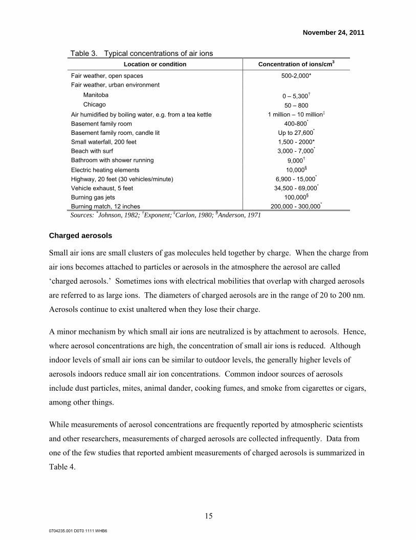
Table 3. Typical concentrations of air ions Location or condition Concentration of ions/cm3
Fair weather, open spaces 500-2,000* Fair weather, urban environment Manitoba 0 – 5,300† Chicago 50 – 800 Air humidified by boiling water, e.g. from a tea kettle 1 million – 10 million‡ Basement family room 400-800* Basement family room, candle lit Up to 27,600* Small waterfall, 200 feet 1,500 - 2000* Beach with surf Bathroom with shower running
3,000 - 7,000*
9,000† Electric heating elements 10,000§ Highway, 20 feet (30 vehicles/minute) 6,900 - 15,000* Vehicle exhaust, 5 feet 34,500 - 69,000* Burning gas jets 100,000§ Burning match, 12 inches 200,000 - 300,000* Sources: *Johnson, 1982; †Exponent; ‡Carlon, 1980; §Anderson, 1971
Charged aerosols
Small air ions are small clusters of gas molecules held together by charge. When the charge from
air ions becomes attached to particles or aerosols in the atmosphere the aerosol are called
‘charged aerosols.’ Sometimes ions with electrical mobilities that overlap with charged aerosols
are referred to as large ions. The diameters of charged aerosols are in the range of 20 to 200 nm.
Aerosols continue to exist unaltered when they lose their charge.
A minor mechanism by which small air ions are neutralized is by attachment to aerosols. Hence,
where aerosol concentrations are high, the concentration of small air ions is reduced. Although
indoor levels of small air ions can be similar to outdoor levels, the generally higher levels of
aerosols indoors reduce small air ion concentrations. Common indoor sources of aerosols
include dust particles, mites, animal dander, cooking fumes, and smoke from cigarettes or cigars,
among other things.
While measurements of aerosol concentrations are frequently reported by atmospheric scientists
and other researchers, measurements of charged aerosols are collected infrequently. Data from
one of the few studies that reported ambient measurements of charged aerosols is summarized in
Table 4.
November 24, 2011
0704235.001 D0T0 1111 WHB6
16
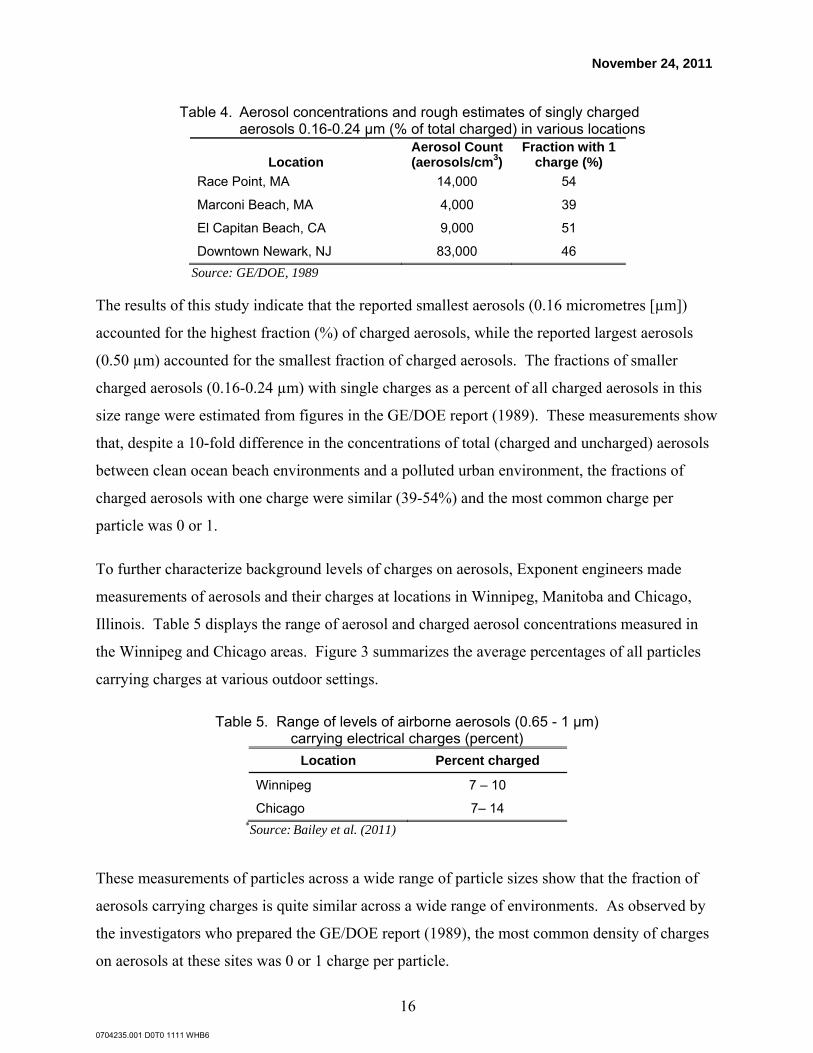
Table 4. Aerosol concentrations and rough estimates of singly charged aerosols 0.16-0.24 µm (% of total charged) in various locations
Location Aerosol Count (aerosols/cm3)
Fraction with 1 charge (%)
Race Point, MA 14,000 54
Marconi Beach, MA 4,000 39
El Capitan Beach, CA 9,000 51
Downtown Newark, NJ 83,000 46 Source: GE/DOE, 1989
The results of this study indicate that the reported smallest aerosols (0.16 micrometres [µm])
accounted for the highest fraction (%) of charged aerosols, while the reported largest aerosols
(0.50 µm) accounted for the smallest fraction of charged aerosols. The fractions of smaller
charged aerosols (0.16-0.24 µm) with single charges as a percent of all charged aerosols in this
size range were estimated from figures in the GE/DOE report (1989). These measurements show
that, despite a 10-fold difference in the concentrations of total (charged and uncharged) aerosols
between clean ocean beach environments and a polluted urban environment, the fractions of
charged aerosols with one charge were similar (39-54%) and the most common charge per
particle was 0 or 1.
To further characterize background levels of charges on aerosols, Exponent engineers made
measurements of aerosols and their charges at locations in Winnipeg, Manitoba and Chicago,
Illinois. Table 5 displays the range of aerosol and charged aerosol concentrations measured in
the Winnipeg and Chicago areas. Figure 3 summarizes the average percentages of all particles
carrying charges at various outdoor settings.
Table 5. Range of levels of airborne aerosols (0.65 - 1 µm) carrying electrical charges (percent)
Location Percent charged
Winnipeg 7 – 10
Chicago 7– 14 *Source: Bailey et al. (2011)
These measurements of particles across a wide range of particle sizes show that the fraction of
aerosols carrying charges is quite similar across a wide range of environments. As observed by
the investigators who prepared the GE/DOE report (1989), the most common density of charges
on aerosols at these sites was 0 or 1 charge per particle.

November 24, 2011
0704235.001 D0T0 1111 WHB6
17
The data in Figure 4 provide greater detail on the data summarized in Table 5. However, the data
in Figure 4 are not directly comparable to the data shown in Table 4 because Figure 4 shows the
fraction of all aerosols that are charged up to 1.0 µm, whereas Table 4 displays the fraction of
smaller aerosols as small as 0.16 µm with 1 charge. In addition, the ranges of aerosol electrical
mobilities measured were not identical.
Figure 4. Fraction of all aerosols (0.65 µm – 1.00 µm) carrying charges in outdoor settings in the vicinity of Winnipeg, Manitoba and Chicago, Illinois.
Ion current density
Ion current density is a phenomenon that can be described as the flow of charge through the air to
the ground (or to grounded objects including people), which is expressed in nanoamperes per
square metre (nA/m2). Ion current density is a function of the electric field and ion
concentration. It is, therefore, of interest because it is a good predictor of surface charge,
including the likelihood that the electric fields and ions can be perceived (i.e., felt by the
movement of hair on the head or arms).
Air quality
In addition to the production of air ions, corona on DC and AC transmission lines also can lead to
the production of trace quantities of ozone (O3). During corona, electrons from the conductor
surface strike neutral gas atoms in the air which may then divide into an electron and a (+) ion.
The electrons are accelerated in the electric field from the conductor and may collide with neutral
oxygen molecules to cause them to disassociate into two negatively charged oxygen atoms.
Ozone is formed when single negative oxygen atoms react with neutral oxygen molecules.

November 24, 2011
0704235.001 D0T0 1111 WHB6
18
Other natural and man-made sources of ozone include sunlight and fuel combustion from cars,
trucks, and factories. Ozone is normally present in the atmosphere in rural areas of Manitoba at
levels of about 20-22 parts per billion (ppb) (Environment Canada, 2008). As a result of research
showing that ozone at high levels can harm lung function and irritate the respiratory system, the
maximum acceptable levels for ozone established by the Canadian National Ambient Air Quality
Objectives is 82 ppb (1 hour basis) for O3 (Health Canada, 2006).
An early study of a ±500-kV DC test line only sporadically detected O3 downwind of the
conductors in wet weather (Droppo, 1979). The most comprehensive study to date performed 2.5
years of pollutant and weather monitoring before and after the construction of a ±400-kV
transmission line in Minnesota. While pollutants were detected in some cases, “the increments
above the background levels were very small and near the detection limits and noise levels of the
monitoring equipment.” Turning the transmission line on and off did not result in detectable
changes in the concentration of pollutants. An increase was only detected when downwind
values were compared to upwind measurements (Krupa and Pratt, 1982). Measurements on a
±450-kV DC test line in Québec did not show a relationship between corona losses on the line
and O3 levels measured downwind (Varfalvy et al., 1985).
Thus, there is no theoretical basis or empirical data to suggest that a DC transmission line would
significantly increase background levels of O3 and adversely impact ambient air quality. As a
result, air quality is not evaluated further in this report.
Audible noise
AN results from the partial electrical breakdown of the air around the conductors of a
transmission line. In a small volume near the surface of the conductors, energy and heat are
dissipated. Part of this energy is in the form of small local pressure changes, which cause AN in
the form of a hissing, crackling, or popping sound.
The conductors of transmission lines are designed to be free of AN under ideal conditions.
Protrusions on the conductor surface (particularly water droplets on or dripping off the
conductors or other debris that settles on the conductors), however, can cause electric fields near
the conductor surface to exceed the levels that cause breakdown of the insulating properties of
the air. The partial electrical breakdown of the air around the conductors of an overhead

November 24, 2011
0704235.001 D0T0 1111 WHB6
19
transmission line produces a dissipation of energy and heat in a small volume near the conductor
surface that changes the sound pressure in the surrounding air. If this small local pressure change
exceeds ambient background levels it may be perceived as AN. DC transmission lines do not
generate substantial AN during fair weather and during foul weather (wet conductors) AN is
attenuated. AN levels are lowered in foul weather (rain or other precipitation) due to the large
increase in ions from the line, an increase caused by the precipitation drops acting as corona
points. The increase in ion density around the line enlarges the effective size of the conductor
and thus lowers AN levels (e.g., larger conductors = lower AN levels). Wet conductors can
occur during periods of rain, fog, snow, or ice.
The amplitude of a sound wave is the incremental pressure difference resulting from sound in
relation to atmospheric pressure. The sound-pressure level is the fundamental measure of AN; it
is generally measured on a logarithmic scale with respect to a reference pressure. The sound-
pressure level (SPL) in decibels (dB) is:
SPLdB = 20 log10 (P/P0)
where P is the effective root mean square (rms) sound pressure and P0 is the reference pressure
of 20 micropascals (µPa), the approximate threshold of human hearing. The human auditory
response depends on frequency, with the most sensitive range roughly between 2,000 and 4,000
Hz. The frequency-dependent sensitivity is reflected in various weighting scales for measuring
AN. The capability to detect noise from the line at residential dwellings was evaluated by
calculating the AN in dB on the A-weighted scale (dB-A). The A-weighted scale weights the
various frequency components of a noise in approximately the same way that the human ear
responds.

November 24, 2011
0704235.001 D0T0 1111 WHB6
20
Table 6. Examples of audible noise levels Sound
Pressure dB-A Condition
140
100 Pa 134 Threshold of Pain
130
Pneumatic Wood Chipper; Jackhammer
120
10 Pa 114 Loud Auto Horn (~ 3’); Rock Concert
110
100
1 Pa 94 Inside Subway Train (NY)
90
Inside Bus
80
100 milli-Pa 74 Traffic on Street Corner
70
Conversational Speech
60
10 milli-Pa 54 Typical Business Office
50
Suburban Living Room
40
1 milli-Pa 34 Quiet Library
30
Quiet Bedroom at Night
20
100 micro-Pa 14 Broadcast Studio
10
20 micro-Pa 0 Threshold of Hearing
Radio noise
Corona caused by high electric field levels at the conductor surface induces impulsive currents
along a transmission line. These induced currents, in turn, cause wideband electric and magnetic
noise fields that can affect radio and television reception. This is experienced as ‘static’
interference with reception of radio signals in the amplitude-modulated (AM) broadcast band
from 535 kHz to 1.605 megahertz (MHz) and, to a lesser extent, television signals in the very-
high-frequency (VHF) band from 54 to 88 MHz. The wideband RN from the proposed Bipole III

November 24, 2011
0704235.001 D0T0 1111 WHB6
21
transmission line can be expected to affect reception under and close to the line, depending on
the broadcast station’s signal strength. Digital television signals and satellite radio signals are
not susceptible to this source of interference. Radio reception in the frequency-modulated (FM)
broadcast band from 88 to 108 MHz is rarely affected. The severity of RN is a function of the
signal strength, noise level, and signal-to-noise ratio and therefore is greatest close to the line and
far from the broadcast antenna.
Like AN levels, RN levels are lowered in foul weather (rain or other precipitation) due to the
large increase in ions from the line, an increase caused by the precipitation drops acting as corona
points.

November 24, 2011
0704235.001 D0T0 1111 WHB6
22
Scientific Reviews and Guidelines
Researchers have been investigating the possible health effects of static electric and magnetic
fields for a very long time. Magnetic fields have been studied more than electric fields because
conducting objects, such as trees and houses, shield electric fields. There has been considerably
less research on long-term health effects (like cancer) and DC magnetic fields compared to the
body of research on AC magnetic fields. This is because static magnetic fields do not induce
currents in stationary objects (such as people or animals). Currents are only induced when there
is motion in the static magnetic field. This type of current induction, however, is not a concern at
the very low levels of magnetic fields produced by the Earth or by DC transmission lines.
The body of research on static fields consists largely of studies on the short-term effects (e.g.,
perception and shocks) of very strong static fields. Research on long-term effects includes
epidemiology studies of workers exposed to static magnetic fields, surveys of residents living
near DC lines, animal studies, and studies in cells and tissues. The best way to understand all of
this research is to rely on the conclusions of the numerous, independent scientific panels that
have evaluated this research using a scientific approach.
Over the past 25 years, there have been a number of reviews of the scientific literature on static
fields by scientific or regulatory organizations. These have included evaluations performed by
the American Conference of Governmental Industrial Hygienists (ACGIH), Health Canada, the
International Agency for Research on Cancer (IARC), the International Commission on Non-
ionizing Radiation Protection (ICNIRP), the International Committee on Electromagnetic Safety
(ICES), the Minnesota Environmental Quality Board (MEQB), the National Radiological
Protection Board (NRPB), the U.S. Food and Drug Administration (FDA), and the World Health
Organization (WHO). The NRPB also reviewed research related to air ions and the MEQB
reviewed the research on air ions and charged aerosols. Figure 5 provides a timeline of these
scientific reviews performed between 2000 and 2010. These reviews, guidelines, and standards
serve as criteria for the assessment of the DC electric and magnetic fields associated with the
proposed project.
In summary, these reviews concluded that experimental studies have established acute sensory
responses associated with high static electric and magnetic fields. Static electric fields can be
November 24, 2011
0704235.001 D0T0 1111 WHB6
23
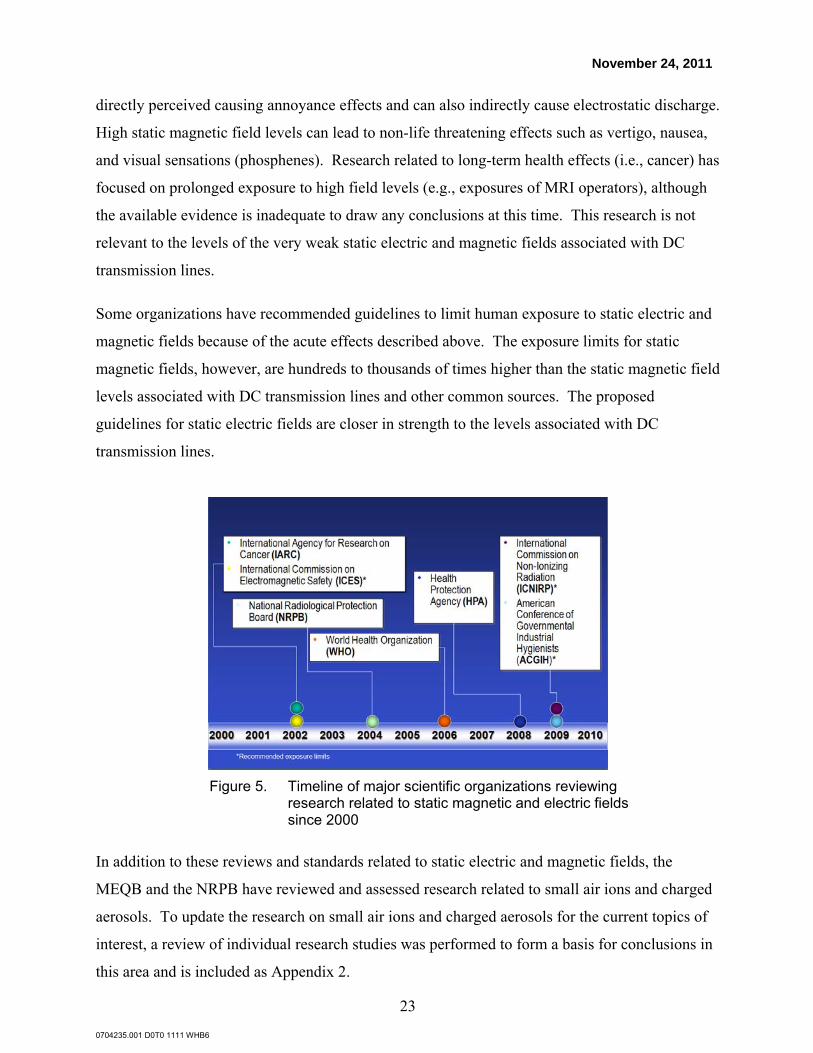
directly perceived causing annoyance effects and can also indirectly cause electrostatic discharge.
High static magnetic field levels can lead to non-life threatening effects such as vertigo, nausea,
and visual sensations (phosphenes). Research related to long-term health effects (i.e., cancer) has
focused on prolonged exposure to high field levels (e.g., exposures of MRI operators), although
the available evidence is inadequate to draw any conclusions at this time. This research is not
relevant to the levels of the very weak static electric and magnetic fields associated with DC
transmission lines.
Some organizations have recommended guidelines to limit human exposure to static electric and
magnetic fields because of the acute effects described above. The exposure limits for static
magnetic fields, however, are hundreds to thousands of times higher than the static magnetic field
levels associated with DC transmission lines and other common sources. The proposed
guidelines for static electric fields are closer in strength to the levels associated with DC
transmission lines.
Figure 5. Timeline of major scientific organizations reviewing research related to static magnetic and electric fields since 2000
In addition to these reviews and standards related to static electric and magnetic fields, the
MEQB and the NRPB have reviewed and assessed research related to small air ions and charged
aerosols. To update the research on small air ions and charged aerosols for the current topics of
interest, a review of individual research studies was performed to form a basis for conclusions in
this area and is included as Appendix 2.

November 24, 2011
0704235.001 D0T0 1111 WHB6
24
American Conference of Governmental Industrial Hygienists
The ACGIH routinely develops guidelines to assist in controlling exposures to potential health
hazards in the workplace. The guidelines are designed to “... provide guidance on the levels of
exposure and conditions under which it is believed that nearly all healthy workers may be
repeatedly exposed, day after day, without adverse health effects” (ACGIH, 2009, p. 1).
The ACGIH did not conclude that exposure to static fields poses a serious health risk (ACGIH,
2009). Its guidelines are based on limiting currents on the body surface (static electric fields) and
induced internal currents (static magnetic fields) to levels below those believed to produce
adverse health effects. For static magnetic fields in the general workplace, whole body exposure
should not exceed 2 Tesla (T) (20,000 G); for trained workers in controlled work environments,
whole body exposures up to 8 T (80,000 G) are permitted on a daily basis. A higher exposure
limit of 20 T (200,000 G) is permitted for the limbs. A magnetic flux density of 20,000 G is
recommended as an overall ceiling value. For static electric fields, the ACGIH found no
convincing evidence that occupational exposure leads to adverse health effects, but
recommended a rms Threshold Limit Value of 25 kV/m (peak = 35 kV/m) to minimize
annoyance from surface fields and nuisance shocks (in dry weather).
Health Canada
Health Canada has published guidelines on short-term exposures of patients and continuous long-
term exposure of operators to the strong static magnetic fields of MRI devices, at 2 T (20,000 G)
and 0.01 T (100 G), respectively (Health Canada, 1987). The panel of scientists assembled by
Health Canada concluded: “On the basis of a number of carefully performed studies, the
following important biological processes appear not to be affected by static magnetic fields up to
approximately 2 T [20,000 G]: (1) cell growth and morphology, (2) DNA structure and gene
expression, (3) reproduction and development, (4) bioelectric properties of isolated neurons, (5)
animal behaviour, (6) visual response to photic stimulation, (7) cardiovascular dynamics, (8)
hematological indices, (9) immune response, (10) physiological regulation and circadian
rhythms” (p. 7).

November 24, 2011
0704235.001 D0T0 1111 WHB6
25
International Agency for Research on Cancer
IARC, the world’s authority on cancer, concluded that the evidence does not support a cause-
and-effect relationship between static magnetic fields or static electric fields and cancer. The
IARC Working Group classified static fields in “Group 3-Not Classifiable” because of
inadequate evidence from either human or animal studies that such exposures cause or contribute
to cancer. IARC defines “inadequate evidence of carcinogenicity” as “The studies cannot be
interpreted as showing either the presence or absence of a carcinogenic effect because of major
qualitative or quantitative limitations, or no data on cancer in experimental animals are
available.” As the WHO later noted, the uncertainty about long-term exposure pertains to static
magnetic fields in the millitesla (mT) range (WHO, 2006a), but not in the range of the Earth’s
geomagnetic field or the range of fields produced by DC transmission lines similar to the
proposed Bipole III project.
International Commission on Non-Ionizing Radiation Protection
Guidelines on static magnetic fields have been proposed by ICNIRP (ICNIRP, 2009). ICNIRP
was established as a continuation of the former International Non-Ionizing Radiation Committee
of the International Radiation Protection Association. The ICNIRP directive is to investigate
hazards that may result from non-ionizing radiation and to protect the public. Their 2004
guideline allowed for the continuous average exposure of the general public to static magnetic
fields at levels below 40 mT (40,000 µT). The NRPB supported these guidelines as a “cautious
approach” (NRPB, 2004b, p. 137). In 2009, ICNIRP increased the limit on public exposure to
static magnetic fields 10-fold to 400 mT (i.e., 400,000 µT [4,000 G]). The effects of concern at
exposures above the limit are induced flow potentials in large blood vessels and vertigo or other
sensory responses caused by currents induced by rapid movements in the field.
International Committee on Electromagnetic Safety
ICES has published an IEEE standard for AC magnetic fields up to 3 kilohertz (kHz) and
magnetic fields at near static frequencies (< 0.153 Hz). The standard is focused on preventing
adverse biological effects from short-term exposures, since the evidence for long-term effects
was not sufficient or reliable.
November 24, 2011
0704235.001 D0T0 1111 WHB6
26
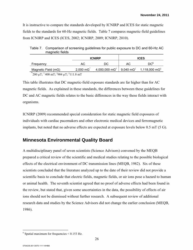
It is instructive to compare the standards developed by ICNIRP and ICES for static magnetic
fields to the standards for 60-Hz magnetic fields. Table 7 compares magnetic-field guidelines
from ICNIRP and ICES (ICES, 2002; ICNIRP, 2009; ICNIRP, 2010).
Table 7. Comparison of screening guidelines for public exposure to DC and 60-Hz AC magnetic fields
ICNIRP ICES
Frequency AC DC AC DC6
Magnetic Field (mG) 2,000 mG* 4,000,000 mG† 9,040 mG‡ 1,118,000 mG§ *200 µT; † 400 mT; ‡904 µT; §111.8 mT
This table illustrates that DC magnetic-field exposure standards are far higher than for AC
magnetic fields. As explained in these standards, the differences between these guidelines for
DC and AC magnetic fields relates to the basic differences in the way these fields interact with
organisms.
ICNIRP (2009) recommended special consideration for static magnetic field exposures of
individuals with cardiac pacemakers and other electronic medical devices and ferromagnetic
implants, but noted that no adverse effects are expected at exposure levels below 0.5 mT (5 G).
Minnesota Environmental Quality Board
A multidisciplinary panel of seven scientists (Science Advisors) convened by the MEQB
prepared a critical review of the scientific and medical studies relating to the possible biological
effects of the electrical environment of DC transmission lines (MEQB, 1982). Six of these
scientists concluded that the literature analyzed up to the date of their review did not provide a
scientific basis to conclude that electric fields, magnetic fields, or air ions pose a hazard to human
or animal health. The seventh scientist agreed that no proof of adverse effects had been found in
the review, but stated that, given some uncertainties in the data, the possibility of effects of air
ions should not be dismissed without further research. A subsequent review of additional
research data and studies by the Science Advisors did not change the earlier conclusion (MEQB,
1986).
6 Spatial maximum for frequencies < 0.153 Hz.

November 24, 2011
0704235.001 D0T0 1111 WHB6
27
National Radiological Protection Board
The NRPB, now a division within the Health Protection Agency of Great Britain, has a long
history of providing support and advice on public health issues relating to ionizing radiation and
electromagnetic fields to the National Health Service, the Department of Health, and other
government bodies in the United Kingdom. The NRPB has issued reviews and assessments on
static electric and magnetic fields and charged aerosols.
In 2004, the NRPB published a comprehensive review of epidemiologic and biological studies
and physical mechanisms of interactions of static electric and magnetic fields and made
recommendations for restricting time-averaged occupational exposures to static magnetic fields
to 200 mT (2,000 G) and the general public’s exposure to 40 mT (400 G) (NRPB, 2004b). These
restrictions are similar to but slightly lower than the guidelines recommended by ICNIRP. This
review and assessment of the magnetic field research was updated in 2008 (HPA, 2008). The
overall conclusion was:
At levels of static magnetic field exposure above about 2 T[esla], [20,000 G] transient sensory effects occur in some individuals; these effects relate at least in part to movement in the field. No serious or permanent health effects have been found from human exposures up to 8 T [80,000 G], but scientific investigation has been very limited. The effects of human exposure to fields above 8 T [80,000 G] are unknown, but some cardiovascular and sensory effects would be expected to increase with stronger fields (p. 3).
The NRPB did not recommend a formal limit on static electric field exposures but noted that
annoying sensations (surface charge perception on body hair) can occur above 25 kV/m (relevant
only to dry weather conditions).
Research on air ions and charged aerosols has also been reviewed by the NRPB. A group of
scientists was assembled to provide input to the Advisory Group on Non-Ionising Radiation
(AGNIR) of the NRPB on the possible effects of corona ions or electric fields on exposure to
airborne pollutants and to address the question of whether corona ions increase the dose of
pollutants to target tissues in the body (NRPB, 2004a). AGNIR examined the hypothesis that a
sufficient amount of charge can attach to pollutant aerosols and increase deposition of the
aerosols. The conclusion of AGNIR was that “the additional charges on particles downwind of
power lines could also lead to deposition on exposed skin. However, any increase in deposition

November 24, 2011
0704235.001 D0T0 1111 WHB6
28
is likely to be much smaller than increases caused by wind.” Their conclusion identified
uncertainties about the inhalation of charged particles, but stated, “However, it seems unlikely
that corona ions would have more than a small effect on the long-term health risks associated
with particulate pollutants, even in the individuals who are most affected. In public health terms,
the proportionate impact will be even lower because only a small fraction of the general
population live or work close to sources of corona ions” (AGNIR, 2004, p. 48). This assessment
has been reaffirmed by the WHO (2007).
A comprehensive review of available research on air ions and respiratory, mood, and behavioral
effects is summarized in Appendix 2 to provide a basis for conclusions in this area. This review
of human exposures to space charge does not suggest effects on the respiratory system, including
those of sensitive persons, and reports of mood-elevation by space charge only have some
support at levels about 10- to 30-fold greater than the levels found under transmission lines, and
cannot easily be distinguished from placebo effects.
U.S. Food and Drug Administration
The FDA’s Center for Devices and Radiological Health has issued guidance to manufacturers
submitting 510 (k) applications for review of MRI diagnostic devices in accordance with 21 CFR
807.87 (FDA, 1998). Per that guidance, exposure up to 4 T (40,000 G) from MRI devices is not
considered a significant risk to patients. This guidance document also recommends that
manufacturers of MRI systems producing a rate of change of the magnetic field (dB/dt) greater
than 20 T/second (200,000 G/second) study and warn operators about dB/dt levels that can
induce peripheral nerve excitation. A labeling guideline is also required for areas surrounding
MRI devices where persons with cardiac pacemakers may be exposed to static magnetic fields
exceeding 0.5 mT (5 G). This guideline is designed to protect against strong attractions of
ferromagnetic materials to the device’s magnet. They also recommended that access be
controlled in areas where magnetic field exposure may result in a potential dysfunction of
ferromagnetic medical implants and electronic medical devices. Evaluations of medical devices
other than MRI devices that produce electromagnetic fields are not assessed with respect to
formally established guidelines, but are assessed on a case-by-case basis. The FDA concluded
that MRI diagnostic devices that emit static magnetic field levels greater than 4 T (40,000 G) for
neonates and 8 T (80,000 G) for adults, children, and infants aged > 1 month are considered to

November 24, 2011
0704235.001 D0T0 1111 WHB6
29
pose significant risk (FDA, 2003). These risk assessment levels are based on clinical studies in
which no significant short-term or persisting effects of exposures to static magnetic fields up to
8 T were reported.
World Health Organization
The WHO has published a comprehensive review of possible health and biological effects of
static fields as an Environmental Health Criteria report (WHO, 2006b). The conclusions were:
Short-term exposure to static magnetic fields in the tesla range [i.e., above 10,000 G] and associated field gradients revealed a number of acute effects (p. 216).
With regard to static magnetic fields, the available evidence from epidemiological and laboratory studies is not sufficient to draw any conclusions about chronic and delayed effects. IARC (2002) concluded that there was inadequate evidence in humans for the carcinogenicity of static magnetic fields, and no relevant data available from experimental animals. They are therefore not at present classifiable as to their carcinogenicity to humans (p. 216).
This conclusion is the same as the earlier IARC (2002) report regarding DC magnetic fields, but
the context for these conclusions is clearer in the WHO document. The range of exposure for
which the WHO identified uncertainty and an insufficiency of evidence is above 0.01 T (100 G)
and, for this reason, the WHO recommended additional research at higher exposure levels. The
WHO further recommended cost-effective precautionary measures that would apply to high field
exposures resulting from the industrial and scientific use of DC magnetic fields (WHO, 2006a;
2006b). An independent review performed for the European Commission by the Scientific
Committee on Emerging and Newly Identified Health Risks (SCENIHR) also concluded that risk
assessments are only necessary with respect to very high occupational exposures to DC magnetic
fields, e.g., from MRI devices (SCENIHR, 2007). The conclusions of this 2007 review were re-
affirmed in an updated opinion by this scientific panel (SCENIHR, 2009).
In their discussion of studies on the effects of static electric field in animals, the WHO concluded
“No evidence of adverse health effects have been noted, other than those associated with the
perception of the surface electric charge” (WHO, 2006b, p. 5). The WHO also noted that the
IARC had not identified any studies of long-term exposure to static electric fields from which
any conclusions on chronic or delayed effects could be made, which rendered the evidence

November 24, 2011
0704235.001 D0T0 1111 WHB6
30
insufficient to determine the potential carcinogenicity of static electric fields. On the whole, the
WHO concluded that “the only adverse acute health effects [related to static electric fields] are
associated with direct perception of fields and discomfort from microshocks” (WHO, 2006b, p.
8).

November 24, 2011
0704235.001 D0T0 1111 WHB6
31
Electrical Environment of Bipole III – Static Fields
Electricity on a DC transmission line is carried over two conductor bundles or ‘poles’ supported
above the ground by insulators suspended on either side of a steel tower. The proposed Bipole
III transmission line will utilize two types of towers. In the northern part of the route, the
transmission line will be constructed on guyed towers in forested areas and other areas that are
compatible with the use of this tower type. In the southern half of the route, through agricultural
areas, the transmission line will be constructed on self-supporting lattice towers. Since the
electrical effects associated with each section of the line are very similar, unless noted otherwise,
all references to electrical parameters will be to calculated values for the line on lattice towers
with typical operating conditions and load. All calculated values referenced in this section are
based upon extensive modeling of the proposed Bipole III transmission line (Appendix 1). For
comparison, the electrical environment of the existing Bipole I and II transmission lines are also
presented in Appendix 1.
The proposed Bipole III transmission line will operate at a constant voltage of ± 500 kV, i.e., the
poles will maintain a (+) or (–) potential with respect to the ground of 500 kV. The maximum
current flow on the Bipole III line typically will be 2,000 amperes (A) when serving a 2,000
megawatt (MW) load.
DC electric field
Each of the poles is a source of a DC electric field, which is identical in nature to naturally-
occurring static fields. The intensity of the electric field is greatest at the conductor surface and
decreases rapidly with distance to the ground. During fair weather, the median electric field
underneath the line will be about 22 kV/m and will increase in foul weather to 30 kV/m. At the
edges of the ROW, the field levels will be much lower in fair (6.5 kV/m) and foul (9.3 kV/m)
weather. During all weather conditions, the electric field decreases sharply with increased
distance from the line. Based on historical weather records for 1990-2004, fair weather prevails
more than 80 percent of the time in Winnipeg and The Pas, but only about 70 percent of the time
further north in Thompson (personal communication. Z. Kieloch). The range of field levels
encountered by the public will be well within the range of commonly encountered background
levels of static electric fields.
November 24, 2011
0704235.001 D0T0 1111 WHB6
32
The potential direct interaction of DC electric fields with humans, animals, and the environment
is limited to the movement of surface charges on the surface of the body; the field does not enter
the body (IARC, 2002). This conclusion is supported by studies of humans and animals exposed
to a wide range of field strengths over varying periods for which no consistent behavioral or
physiological responses are noted except those related to field perception. At sufficiently high
levels, an electric field can be sensed by the movement of body hair. A psychophysical study of
the ability of human subjects under carefully controlled conditions to detect a static electric field
reported a range of perception thresholds, but the average critical detection value was 40.1 kV/m.
When the ion current density was simultaneously raised to 120 nA/m2 (1.33 x 10⁵ ions/cm3), the
threshold was lowered to 25 kV/m (Blondin et al., 1996). Testing done outdoors under DC
transmission lines indicates that most persons would not detect electric fields at levels less than
about 25 kV/m (Clairmont et al., 1989; NRPB, 2004a).
As described above, the NRPB has recommended 25 kV/m as the general public limit for DC
electric fields (NRPB, 1994). A similar value has been recommended as a Threshold Limit
Value for occupational exposures (ACGIH, 2009). A higher value of 42 kV/m was
recommended as an upper limit (basic restriction) in an earlier Comité Européen de
Normalisation Électrotechnique pre-standard (CENELEC, 1995).
In fair weather, the calculated DC electric fields of Bipole III will be below the lowest
recommended limit of 25 kV/m. In foul weather, in which persons are less likely to be on the
ROW, the DC electric fields may exceed this value within portions of the ROW, although the
likelihood of field perception would not expected to be increased because perception results from
the movement of hair on the head and body and the body surface would likely either be covered
by clothing or wet during foul weather.
Unlike AC electric fields, DC electric fields are not capable of coupling effectively to conductive
objects and so the current density intercepted by a person under a DC transmission line is on the
order of a few microamperes, which is below the threshold for detection of DC currents. Even
for large vehicles parked underneath a DC transmission line or long parallel fences, the charge
collected is limited by leakage current to the ground so the possibility of perception is limited;
under experimental ‘worst case’ conditions, the only noticeable effect of touching a large, well
grounded vehicle would be a microshock, weaker than what a person might experience after
shuffling across a carpet. This finding has been confirmed for Bipole I and II (Maruvada et al.,

November 24, 2011
0704235.001 D0T0 1111 WHB6
33
1982) and DC test lines (EPRI, 1978).
DC magnetic field
The magnetic field that will be produced by the proposed Bipole III transmission line is identical
to the geomagnetic field of the Earth. The strength of this natural field in Manitoba is about 580
mG. Since magnetic fields are vectors, the magnetic field from the line will add to that of the
Earth’s geomagnetic field when the vectors are pointing in the same direction, and it will
partially cancel the Earth’s geomagnetic field where the magnetic field vectors of the DC lines
point in the opposite direction. The result is that the measured magnetic field will be increased
above background levels on one side of the ROW and will be decreased below background levels
on the other side of the ROW. Outside the ROW, there will be an insignificant change in the
background geomagnetic field. The contribution of the transmission line to this background field
will be less than 405 mG in bipolar or monopolar operation even under the heaviest expected
normal load.
Biological and health studies involving exposure of humans and multiple species to DC magnetic
fields have been performed for over one hundred years. Evaluations of this research have been
commissioned by a number of scientific agencies. These reviews and the resulting standards are
described in detail in the section Scientific Reviews and Guidelines above. The ICNIRP has
published reviews of biological effects and mechanisms (Matthes et al., 1997, 2000). The IARC
concluded that the data did not deserve classification as a potential carcinogen and described
static magnetic fields as not classifiable (Group 3) (IARC, 2002). Based on a review that
included more recent studies of human subjects exposed to strong static magnetic fields from
MRI devices and an evaluation of known mechanisms of interaction, ICNIRP recommended that
the maximum exposure of the general public be increased from 40 mT to 400 mT, which is
equivalent to 4,000 G (ICNIRP, 2009). Health Canada has published guidelines on short-term
exposures of patients and continuous long-term exposure of operators to the strong static
magnetic fields of MRI devices, at 2 T (20,000 G) and 0.01 T (100 G) respectively. Both the
Earth’s geomagnetic field and the magnetic field from the proposed Bipole III transmission line
are hundreds to thousands of times lower than these limits.

November 24, 2011
0704235.001 D0T0 1111 WHB6
34
Electrical Environment of Bipole III – Space Charge
Air ions
A transmission line is “in corona” when the strength of the electric field at the conductor surface
exceeds a threshold or onset level of approximately 30 kV/cm. The calculated electric field
gradient along the span of the proposed Bipole III conductors is below the threshold for corona
onset (i.e., approximately 22.4 kV/cm); however, the presence of minor imperfections in the
conductor surface (i.e., nicks, scratches, dust contamination, insect contamination, and ice, snow,
or water droplets) can cause the electric field to be concentrated at these points and exceed this
threshold producing corona. The energy released by corona discharge can lead to air ions.
Air ions around DC transmission lines have been well characterized by measurement and
calculations. Appendix 1 describes the air ion levels expected from the proposed transmission
line. Corona discharge on the Bipole III line conductors will produce varying levels of small air
ions at the ground that are highest under the conductors and lower at the edges of the ROW. The
rapid reduction in ion concentration is explained by the movement of the ions of one polarity to
the opposite conductor and to the ground by the electric field where the charge is neutralized.
Outside the ROW, the electric field is much weaker and so the transport of the ions by wind
tends to disperse the ions higher in the air rather than force them to the ground. When the wind
blows strongly across the transmission line, the shape of the air ion and electric field distributions
will be shifted, reducing values on the upwind side and increasing values on the downwind side.
The calculated median level of air ions at the edge of the ROW is 20,000 ions/cm3 or less, with
lower values in fair weather. These values are higher than ambient background levels measured
outdoors but within the range of exposures encountered from common sources (Table 8).
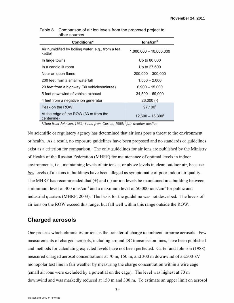
November 24, 2011
0704235.001 D0T0 1111 WHB6
35
Table 8. Comparison of air ion levels from the proposed project to other sources
Conditions* Ions/cm3
Air humidified by boiling water, e.g., from a tea kettle† 1,000,000 – 10,000,000
In large towns Up to 80,000
In a candle lit room Up to 27,600
Near an open flame 200,000 – 300,000
200 feet from a small waterfall 1,500 – 2,000
20 feet from a highway (30 vehicles/minute) 6,900 – 15,000
5 feet downwind of vehicle exhaust 34,500 – 69,000
4 feet from a negative ion generator 26,000 (-)
Peak on the ROW 97,100‡
At the edge of the ROW (33 m from the centerline) 12,600 – 16,300‡
*Data from Johnson, 1982; †data from Carlon, 1980; ‡fair weather median
No scientific or regulatory agency has determined that air ions pose a threat to the environment
or health. As a result, no exposure guidelines have been proposed and no standards or guidelines
exist as a criterion for comparison. The only guidelines for air ions are published by the Ministry
of Health of the Russian Federation (MHRF) for maintenance of optimal levels in indoor
environments, i.e., maintaining levels of air ions at or above levels in clean outdoor air, because
low levels of air ions in buildings have been alleged as symptomatic of poor indoor air quality.
The MHRF has recommended that (+) and (-) air ion levels be maintained in a building between
a minimum level of 400 ions/cm3 and a maximum level of 50,000 ions/cm3 for public and
industrial quarters (MHRF, 2003). The basis for the guideline was not described. The levels of
air ions on the ROW exceed this range, but fall well within this range outside the ROW.
Charged aerosols
One process which eliminates air ions is the transfer of charge to ambient airborne aerosols. Few
measurements of charged aerosols, including around DC transmission lines, have been published
and methods for calculating expected levels have not been perfected. Carter and Johnson (1988)
measured charged aerosol concentrations at 70 m, 150 m, and 300 m downwind of a ±500-kV
monopolar test line in fair weather by measuring the charge concentration within a wire cage
(small air ions were excluded by a potential on the cage). The level was highest at 70 m
downwind and was markedly reduced at 150 m and 300 m. To estimate an upper limit on aerosol

November 24, 2011
0704235.001 D0T0 1111 WHB6
36
charging, Johnson and colleagues subsequently took measurements around a test line designed to
produce ion levels two to three times greater than a typical DC transmission line. They found
that the distribution of charges was bipolar with a slight predominance of (-) charges out to
200 m downwind. The most common number of charges (i.e., charges/aerosol) was a single
charge. Carter and Johnson also took spot measurements downwind of the Pacific Intertie ±500-
kV transmission line in California, which showed similar results (GE/DOE, 1989). Overall,
while a small effect of these DC sources could be measured, the fraction of aerosols with charges
was similar to, but sometimes slightly higher or lower, than measured in other environments
(Table 4).
To obtain additional information about the effect of DC transmission lines on charged aerosol
levels, Exponent engineers made measurements in rural Manitoba around the corridor on which
the Bipole I (±450-kV) and Bipole II (±500-kV) DC transmission lines operate (Bailey et al.,
2011). These lines are separated by about 65 m. The results are shown in Figure 6.
Figure 6. Charged aerosol fraction (%) with respect to distance from the centerline of the ±450-kV and ±500-kV transmission lines in Manitoba

November 24, 2011
0704235.001 D0T0 1111 WHB6
37
The fractions of aerosols carrying (+) and (-) charges with selected mobilities within the range of
4.14 x 10⁻⁷ m2/V·s and 9.64 x 10⁻¹⁰ m2/V·s were measured at sites upwind and downwind of the
lines. Measurements made at times when the wind was blowing from both directions during the
measurement period (labeled “variable”) are also shown. The average fractions of particles with
charges within 500 m from the centerline were 5-10% at downwind locations, 6-12% at upwind
locations, and 1-6% at locations when the wind direction varied. The fractions of charged
aerosols at this site are similar to measurements taken at a variety of locations at a distance from
a DC transmission line, as previously shown in Figure 4, and also commonly carried 0 or 1
charge per particle.
More detailed analyses were carried out on the distribution of charge on aerosols measured
around the Bipole I and II transmission lines and the results are shown in Bailey et al. (2011). In
summary, the fractions of aerosols carrying charge upwind and downwind were similar but the
polarity of the charges downwind was shifted. Upwind the charges on aerosols were about
equally likely to be (+) or (-), but downwind the number of aerosols with (+) charge was reduced
relative to those carrying (-) charges. Slightly more aerosols with multiple charges were
observed 90 m downwind than 90 m upwind and this difference appeared less at 490 m
downwind. Nevertheless, both upwind and downwind of the lines the modal distribution was one
charge per aerosol and almost all aerosols carried 10 or few charges. The number of charges on
aerosols measured around the DC lines was very similar to that measured at four locations
around Winnipeg and four locations around Chicago.
The data provide no indication that the two DC transmission lines in Manitoba substantially
increase the number of aerosols bearing charges over background levels. Furthermore, neither
the measurements made around Bipole I and II nor the measurements of test lines (GE/DOE,
1989) suggest that DC transmission lines lead to many more aerosols with a large number of
charges per particle. Thus, the levels of charged aerosols around DC transmission lines do not
appear to differ in any meaningful way from other ambient environments.

November 24, 2011
0704235.001 D0T0 1111 WHB6
38
Electrical Environment of Bipole III – Audible Noise and Radio Noise
Additional corona phenomena
The energy released by corona discharge can also lead to AN, RN, and visible light. Appendix 1
describes the AN and RN levels expected from the proposed DC transmission line.
Audible noise
The median AN level on the ROW in fair weather is 39 dB-A and this diminishes to about 36
dB-A at the edge of the ROW. These values are within the range of values expected in quiet
rural and suburban areas.
Manitoba’s Provincial Guidelines specify maximum desirable 1-hour equivalent noise levels for
both residential and commercial areas of 55 dB-A and 45 dB-A, for day-time and night-time
periods, respectively (EMD, 1992). These standards will be met by Bipole III in fair weather
even under the conductors on the ROW. In foul weather, the levels of AN will be about 6 dB-A
lower and will typically be masked by noise from wind and rain.
Radio noise
The Industry Canada standard for RN for a 500-kV transmission line is 60 dBμV/m at 15 m from
the nearest conductor that would be measured by a CISPR-type measuring instrument according
to CSA Standard C108.1.1-1977 (Industry Canada, 2001). This standard will be met by the
proposed Bipole III transmission line within the ROW and beyond in fair weather; the levels will
be even lower in foul weather.
Visible light
The ejection of electrons with low energy from the conductor surface during corona increases the
energy levels of surrounding gas molecules, which when released gives rise to AN and RN as
described above and a faint bluish light. The light produced is so weak that it typically can only
be seen at night, particularly under foul weather conditions, and even then special binoculars or
other magnification may be required to detect the light.

November 24, 2011
0704235.001 D0T0 1111 WHB6
39
Interference with electronic devices
Global Positioning System receivers
GPS is a space-based navigation system that relies on 24 orbiting satellites circling the Earth to
establish the position of a GPS receiver on the Earth. The receiver uses the radiofrequency (RF)
signals sent from three or more of these satellites to determine its exact location. Naturally-
occurring sources of RF (e.g., geomagnetic storms) and man-made sources of RF (e.g., TV
station transmitters) are sometimes reported to interfere with GPS signals because these sources
can produce interference in the same frequency ranges as used by GPS. Since GPS signals are of
far higher frequency than the RN of a DC transmission line, it is very unlikely that a DC
transmission line will interfere with GPS functioning.
Modern GPS receivers can receive corrections from a number of satellite-based systems with
frequencies above 1 gigahertz (GHz) to improve the accuracy of positional location; this is called
differential GPS (DGPS). Some GPS systems also make use of real-time kinematic (RTK)
systems to improve the accuracy of the GPS system by making use of the ultra high frequency
(UHF) range. Since the frequency bands of these systems are far higher than RN frequencies of
concern produced by a DC transmission line, signal interference is unlikely to occur. Since the
GPS signal at ground level is very weak, it is possible that some receiver designs may be
susceptible to minor interference due to certain factors. Conceptually, a DC transmission line
might affect GPS performance in two additional ways: (1) RN interference to Nationwide
Differential GPS (NDGPS) positional corrections and (2) signal blocking and reflection. These
concepts are described further below.
Nationwide differential GPS positional correction
NDGPS is a GPS system commonly used in the United States and along the southern border of
Canada that was developed to improve GPS accuracy when GPS first became available. This
system works together with a GPS system making use of land-based towers to transmit correction
signals to GPS receivers. NDGPS uses lower frequencies to send correction signals. These
lower frequency signals can overlap with the RN frequencies discharged from a DC transmission
line. The likelihood of interference in each situation will depend on the GPS receiver’s distance
to the transmission line, as well as its distance to the closest NDGPS antenna. A momentary loss
of NDGPS signal, however, should not substantially affect the accuracy of the overall positioning
November 24, 2011
0704235.001 D0T0 1111 WHB6
40
system. The accuracy of GPS signals is much greater today and therefore the NDGPS positional
correction does not substantially improve the accuracy of current GPS receivers, which have an
accuracy of a few metres. Canada terminated support for NDGPS on April 1, 2011 and
alternatives to Canada-Wide DGPS Service provide corrections signals for land receivers by
mobile satellite (MSAT) or UHF cellular radio (CDGPS, 2011), which are not or minimally
susceptible to RN interference from transmission lines.
Signal blocking and reflection
RF signals can be blocked by physical objects (e.g., mountains) or degraded by reflections off
large solid objects. The towers of a DC line, while relatively large compared to the size of a
person, for example, do not have a large footprint and they are not solid. So while the towers can
result in some reflections and blocking of RF signals their impact is generally momentary and
insignificant. Transmission line conductors are also too thin to block or cause large reflections of
RF signals. GPS and related receivers are typically configured to reduce the effects of blocked
and reflected signals, resulting in a very small and temporary blockage area if it occurs. Further,
the concept of multiple satellite options implies that having the signal from one of a group of
satellites blocked is not consequential since the reception from the other satellites is still
available.
GPS use in agriculture
As described, RN from a DC transmission line would not be expected to directly affect GPS
signal reception or the reception of satellite-based positional correction signals used in equipment
for farming operations. Since RTK correction signals are transmitted from antennas that are
typically only a few metres high, DC transmission line towers are not expected to produce much
blocking of line-of-sight signals from these sources either. Repositioning of the RTK base
station antenna should resolve any issues if they occur. Signal degradation can occur due to
reflections from a nearby flat-topped building or other reflecting surfaces (such as lakes). The
overall performance of a GPS guidance system in agriculture depends upon a high-quality
receiver, proper mounting, and good positional correction from an independent source.

November 24, 2011
0704235.001 D0T0 1111 WHB6
41
Tests for DC transmission line interference to GPS
Manitoba Hydro has been questioned as to whether the presence of Bipole III will interfere with
GPS systems. The RN from DC transmission lines is low intensity and occurs at frequencies that
are far lower than those used by GPS systems. Because of this, the DC transmission line will not
interfere with GPS signals. Manitoba Hydro requested field testing in order to confirm this
conclusion. Two surveys by independent surveyors were performed using various types of GPS
technologies directly beneath the two existing Bipole I and II DC transmission lines located in
Manitoba’s Interlake region (Pollock & Wright, 2010; Plan Group, 2011). The tests showed no
interference whatsoever with any type of GPS or Global Navigation Satellite System (GNSS)
technology tested, including RTK and other correction systems. The GPS receivers tested
continued to operate without interruption at cm accuracies regardless of the presence of the DC
transmission lines. In theory, the presence of the transmission towers themselves might
occasionally attenuate satellite signals related to GPS systems (as do trees) but this was not
observed during testing. A GPS receiver makes use of multiple satellites in determining its
position and so the loss of one or even two of these signals will not normally result in a loss of
function of the GPS systems. A limited series of measurements under a nearby 230-kV AC
transmission line also did not affect the performance of the GPS receivers (Pollack & Wright,
2010).
Mining surveying equipment
Whether the electromagnetic fields from the proposed Bipole III transmission line will interfere
with mining exploration survey methods depends on the distance to the line, the type of
measurement equipment used for the explorations, and post-processing corrections of the
acquired data. The primary methods of acquiring data involve:
1. Mapping the geomagnetic field and anomalies associated with ore deposits with very
sensitive magnetometers (claimed sensitivity is 0.01 nanotesla [nT]; practical sensitivity is
0.1 nT) by ground or aerial surveys.
2. Applying time-domain AC or pulsed magnetic fields to the ground and then measuring the
signal dB/dt during or after the collapse of the impressed magnetic field, or both. Improved
resolution is achieved by placing receiver probes down in boreholes closer to conducting ore

November 24, 2011
0704235.001 D0T0 1111 WHB6
42
deposits. These methods might also include measurements of weak electromagnetic fields
induced in the Earth by the ionosphere or from thunderstorm activity.
3. Injecting currents into the ground through electrodes and measuring the pattern of
conductivity around the electrodes.
Aeromagnetic surveying relies on an accurate measurement of the DC magnetic field from the
ground to enable correction for the effects of the DC magnetic field from the transmission line.
Measurement sensitivity is typically 0.1 nT after correction of time-dependent fluctuations of the
magnetic field such as diurnal fluctuations (50 nT to 100 nT) and micropulsations (0.001 nT to
10 nT). Natural, magnetically-induced currents that produce magnetic fields can vary by as
much as 10 nT/second, which will also affect the measurements (Pirjola, 2000). Rough estimates
suggest that Bipole III might affect the DC magnetic fields to a level at or above 0.1 nT out to
distances of up to about 8 to 10 km on either side of the line.7
Electromagnetic surveys, such as a Helicopter Electromagnetic (HEM) survey, do not rely on the
Earth’s natural magnetic field, but rather rely on the time and frequency response of the ground
to the magnetic pulses generated by the airborne coil. Such HEM surveys have been utilized
before in nickel-copper sulphide deposit exploration (Balch, undated). These measurements
would not be affected by the DC magnetic field from Bipole III, but may be affected by the AC
electric fields or magnetic fields associated with harmonic AC currents injected into the line by
the converters at the ends of the line. Harmonic filters normally are installed at the ends of the
DC transmission line to reduce the magnitude of the injected currents. Typical performance
specifications for such filters are to limit the induced voltages to between 10 and 20 millivolts
(mV) as measured in a 1 km test line placed in parallel with the line at a distance of 1 km from
the line. The specified value typically is defined with a C-weighted average used for the
evaluation of telephone interference.
Electronic medical devices
Pacemakers
The magnetic field from a DC transmission line is too weak to affect cardiac pacemakers. Since
the background level of the static magnetic field in Manitoba is approximately 580 mG and the
7 Under rare emergency operating conditions, this effect could be extended.

November 24, 2011
0704235.001 D0T0 1111 WHB6
43
maximum increase from Bipole III is estimated to be about 50% above this background, the
exposures to a person with an implanted pacemaker even under the transmission line will be far
below the recommended limit of 0.5 mT (5,000 mG) (ACGIH, 2009).
Similarly, the static electric field from a DC line would not be expected to be a source of
interference to a pacemaker. In theory, a pacemaker might be affected by an electrostatic
discharge directly to the chest from a large well-insulated, ungrounded vehicle, e.g., a tractor-
trailer, under a DC transmission line. The short duration of such a discharge, however, and the
insulation from the ground necessary to accumulate such a charge makes it unlikely to affect a
pacemaker (Stuchly and Kavet, 2005). Such an exposure might occur in some occupational
environments but the magnitude, distribution, and conditions for the electric field under the
Bipole III DC transmission line makes this exposure scenario less likely than exposure from the
static electric field commonly associated with certain clothing in the winter.
Cochlear implants
For some persons with severe hearing loss, a cochlear implant can provide partial hearing. The
device consists of a small microphone behind the ear that provides complex processing of the
sound into digital electrical signals that are then transmitted over an array of wire electrodes
surgically implanted in the cochlea, the auditory portion of the inner ear. The signals bypass
non-functional hair cell receptors to directly stimulate the auditory nerve which is perceived as
sound.
A question was raised as to whether the electric field and space charge from the proposed Bipole
III transmission line would cause an electrostatic discharge sufficient to interfere with the device.
To address this question, it was assumed that the cochlear implant has been tested for
electromagnetic immunity as set forth in the IEC 60601-1-2 medical electrical equipment
standard (IEC, 2001). As recommended in IEC 60601-1-2, immunity testing of cochlear devices
to electrostatic discharge (ESD) should be tested to IEC 61000-4-2 levels that specify immunity
levels of 6 kV to a contact discharge exposure and 8 kV to an air discharge exposure (EMC,
2000; Chute and Nevins, 2002; Tognola et al., 2007). Some manufacturers also test at higher
immunity levels (Tognola et al., 2007).
Assuming the presence of a 150 nA/m2 ion flux density, which is higher than expected under the
Bipole III transmission line under emergency loading condition, and based on published values

November 24, 2011
0704235.001 D0T0 1111 WHB6
44
of the DC resistance to the ground of persons wearing shoes, standing under the Bipole III
transmission line will not develop human-body potentials that would exceed the IEC immunity-
test levels for a cochlear implant. The method of this analysis can be explained with reference to
Figure 6.
Figure 7. Charging model for person standing under the Bipole III line
Iflux represents the ion current collected by a person standing beneath the conductors of the Bipole
III transmission line. Iflux develops an electric potential on surface of the body (Vbody) by charging
the body’s capacitance (Cbody). Charge collected on the body surface returns to the ground
through the leakage resistance Rleakage, which models the DC impedance of footwear in contact
with the Earth.
In steady state, the charging current (ion flux) and discharging current (leakage) are equal, and
the potential of the human body does not change. This steady-state potential is the maximum
sustained voltage that can be developed on the body the under the transmission line. A person
wearing dry, new boots and standing on dry ground will have a higher leakage resistance, lower
discharging current, and a higher steady-state body potential. Conversely, a person wearing wet,
soiled boots and standing on damp grass will have a lower leakage resistance, higher discharging
current, and a lower steady-state body potential.
Iflux
Rleakage Vbody Cbody

November 24, 2011
0704235.001 D0T0 1111 WHB6
45
A conservative estimate of the ion flux density under the Bipole III transmission line is 150
nA/m2, i.e., for each square metre of collection area, space charge from the overhead
transmission line collects at a rate of 1.5×10⁻⁷ coulombs per second.8
The collection area of a person 6 feet in height is calculated to be 5.6 m2 based on published AC
induction expressions for the human body. In particular, the short-circuit induced current Isc for a
person is reported by the Electric Power Research Institute (EPRI, 2006) as
(1)
where h is height in m, and E is the unperturbed electric field in units of V/m. Expression (1) is a
specific form of the more general expression
(2)
where jω is the angular frequency in radians per second (377 rad/s), ε is the permittivity of free
space (8.85×10⁻¹² F/m), and S is the collection area of a charging object in units of m2. Solving
(1) and (2) for S, the collection area of a person increases with height according to the expression
(3)
where h is height in m, S = 5.6 m2 for a person 1.85 m (6 feet) tall. The total current Iflux is the
product of the charge collection area and ion flux density. Based on the parameters above, Iflux =
833 nA, less than one-millionth of one A.
Rleakage is estimated by the DC resistance of persons in shoes, as reported by Reilly (Reilly 1998a,
1998b). Figure 7, reproduced from these sources, is explained by the author as follows:
Footwear can add significantly to the total path resistance, as illustrated in [Figure 7]. This figure plots the distribution of DC resistance on individuals standing on various surfaces, with a current pathway from a large electrode held in the hand, to a nearby driven ground rod in the soil. The measurement voltage was 500 V. In all cases, footwear was dry, except for surface moisture on which the person stood. In general, leather soles are much more conductive than rubber soles. If leather soles become wet, their resistance can fall greatly. Grass blades that touch the sides of the shoes can also significantly lower their resistance. The curves labeled “damp grass” apply to individuals standing on short grass; in the “wet
8 For air ion concentrations of 130 thousand ions/cm3 calculated for the Bipole III transmission line, 150 nA/m2
charging current corresponds to a 7.2 m/s ion drift velocity in the DC electric field beneath the DC conductors.

November 24, 2011
0704235.001 D0T0 1111 WHB6
46
grass” condition, subjects first stood briefly on 1cm of water before stepping on the grass. In tall grass (e.g., 8cm), we would except to see much larger percentages of low resistances.
Figure 7 shows that all measurements of DC leakage resistance were less than 2 giga-ohms (GΩ).
Hence, 2 GΩ was used as a conservative upper bound on Rleakage.
Using the parameters described above, the potential rise Vbody of a person standing beneath the
transmission-line conductors is Rleakage· Iflux = 1.6 kV, a value 3.75 times lower than the IEC
immunity test level of 6 kV. It should be noted that this result is conservative in at least two
respects:
1. parameters in the charging model (Figure 6) are a conservative estimate of actual
parameters; and
2. the 6 kV immunity test level is applied directly to the medical device, whereas contact
currents and charging in the human body do not—in many circumstances—electrically stress
an implanted device directly.

November 24, 2011
0704235.001 D0T0 1111 WHB6
47
Figure 8. DC resistance of persons through shoes, standing on various surfaces (reproduced from Reilly 1998a, 1998b)

November 24, 2011
0704235.001 D0T0 1111 WHB6
48
Dairy Cattle, Wild Animals, and Plants
Dairy cattle and DC transmission lines
Two studies have been conducted to respond to the concerns of farmers about possible effects of
the electrical environment of DC transmission lines on dairy cattle. The first study was
conducted by investigators at the University of Minnesota who used the records of the Dairy
Herd Improvement Association to study the health and productivity of approximately 500 dairy
herds (about 24,000 cows) from farms located near the ±400-kV CPA/UPA DC transmission line
in Minnesota (Martin et al., 1983). Veterinary records for a 6-year period were examined, from
3years before to 3 years after energization of the line in 1979. The herds were grouped according
to distance of the farmstead from the transmission line, with the closest herds less than 0.25 miles
(400 m) from the line, and the farthest between 6 and 10 miles (~10 to 16 km).
Endpoints selected for study included milk production per cow, herd average of milk production,
milk fat content, and measures of reproductive efficiency, among others. The health and
productivity of the herds was found to be the same before and after energization and also was
found to be unrelated to distance of the herds from the transmission line.
In another study, investigators at Oregon State University compared the health and productivity
of 200 cow-calf pairs randomly assigned to pens directly under or 615 m away from the Pacific
Intertie ±500-kV DC transmission line. No differences between the animals in the exposed and
control pens were noted with regard to breeding activity, conception rate, calving, calving
interval, body mass of calves at birth, body mass at weaning, or mortality over a 3-year period.
The average exposure of the animals in pens under the line was about 5 kV/m and 13,000
ions/cm3 (Angell et al., 1990). As part of this study, the investigators also monitored the
activities of the exposed and control cattle at 15-minute intervals during a 24-hour period each
month (Ganskopp et al., 1991). The distribution of cattle along feed troughs in the exposed and
control pens was similar and unrelated to measures of the static electric field and there were no
major differences in the time spent in various behaviors. Although small differences in the
distribution of cattle within the pens were noted, the investigators reported that the differences
were not correlated with fluctuations in the static electric field or AN levels.

November 24, 2011
0704235.001 D0T0 1111 WHB6
49
Plants
The studies performed on plants exposed to DC magnetic fields have predominantly focused on
effects on genetic, growth, and enzymatic activities. No adverse genetic effects were reported
(McCann et al., 1993) and the results of studies on growth were inconsistent (Simon, 1989).
A substantial amount of laboratory research has been performed on the effect of air ion exposure
on plants. This research, like that associated with air ion research on animals and humans,
consists of a few responses that have not been replicated and that are of questionable quality.
Most of the work studying the effect of air ions on several types of plants, including oat and
barley, was performed under the direction of Krueger and co-workers. They reported a
significant increase in the plants’ dry weight (Krueger, et al., 1962, 1963) when exposed to
concentrations ranging from 5,000 ions/cm3 to 13,000 ions/cm3. Other investigators found that
plants grown in ionized air showed enhanced fresh weights along with enhanced growth, but no
change in dry weights (Wachter and Widmer, 1976). An explanation for this observation is that
the increase in growth was at the expense of the existing plant mass. Similar reports of enhanced
growth, fruit yield, and quality are reported for tomato plants exposed to air ions at levels in the
range of 10,000 ions/cm3 (Yamaguchi and Krueger, 1983).
When seedlings of barley are cultivated in an iron-deficient nutrient medium, they eventually
develop an iron deficiency. Krueger et al. (1963, 1964) reported that iron deficient seedlings
cultivated in an atmosphere of air ions, either (+) or (-) polarity, biochemical indicators
associated with iron deficiency were increased. This may merely reflect, however, the greater
demand for iron in a more rapidly growing seedling that had been exposed to air ions, which was
also reported (Krueger et al., 1963).
Several studies have examined the effect of DC transmission lines on plants and are more
relevant to real world circumstances than observations made in a laboratory setting. An
outdoor test facility in Japan was designed to examine the possible effects of a DC power line
on the growth of wheat plants positioned at 3 m, 4.5 m, and 6 m below the conductors under
the +100kV and -100-kV conductors (Endo et al., 1979). The electric field intensities were
calculated to be 42 kV/m, 65 kV/m, and 84 kV/m, respectively at the above designated line
heights. The investigators concluded that there were “no significant differences” between the

November 24, 2011
0704235.001 D0T0 1111 WHB6
50
control and exposed plants with regard to development and differentiation, but in the last
month of the growing season the heights of plants under the conductors were 5% lower than
control plants and 12-26% fewer tillers were measured on exposed plants. Differences among
plants in the exposed group, however, were not clearly related to differences in the strength of
the applied electric field. Even with these observed differences between exposed and control
plants, the harvest yield or composition of the stems or seeds was not reported to be affected.
Crops on the ground under the proposed Bipole III transmission line would be 13 m below the
conductors, not 3-6 m as in this study, and the maximum electric field will be significantly
lower than in the Endo et al. (1979) study.
Krupa and Pratt (1982) surveyed the growth, condition, and disease incidence in crops grown in
25 plots located 30.5 m from the centerline of a ±400-kV DC transmission line. No effects
attributable to the presence of the line (including exposures to O3 or to electric or magnetic
fields) were detected based upon reference data of the local Animal and Plant Health Information
System.
The above research on plants provides some indication that plants in laboratory conditions may
exhibit enhanced growth in response to varying levels of air ions, but further research is needed
to confirm such observations and to determine the potential mechanism. The evidence for
responses of plants to other aspects of the DC transmission environment, i.e., the electric field
and magnetic field, is not sufficient to conclude these exposures have any reliable influence on
plants.
Wild animals
Griffith performed a study to investigate the effect of the Pacific Intertie DC transmission line in
Oregon on the plant and animal communities when operating at ±400 kV (Griffith, 1977). He
performed systematic sampling of these populations with primary emphasis on crops, natural
vegetation, songbirds, raptors, small mammals, pronghorn antelope (Antilocapra americanca),
and mule deer (Odocoileur hemionus). There were some species that were influenced, either
positively or negatively, by the presence of the transmission line. Overall, species that were
negatively influenced were those that needed undisturbed plant species, or have some specialized
type of behavior with which transmission line structures interfere, such as robins, Brewer's
sparrows, and pinon mice. Those species that were positively affected used the transmission line

November 24, 2011
0704235.001 D0T0 1111 WHB6
51
structures as part of their feeding, hunting, or resting habitats, including certain types of raptors
and Townsend’s ground squirrels. The observed impacts were believed to be related to the
physical presence and construction of the line rather than the electrical environment associated
with the line. It is not possible, however, to conclude from this study alone that all observed
differences were the result of the physical change to habitat by construction of the line.
The Earth’s geomagnetic field has been shown to be detected by a variety of organisms ranging
from bacteria to homing pigeons (Kirschvink, 1982). A change in the intensity or orientation of
the Earth’s geomagnetic field has been reported to affect orientation or navigational clues that are
used by some animals.
Blakemore demonstrated that certain anaerobic bacteria swim to the North Pole in the northern
hemisphere, the South Pole in the southern hemisphere, and in both directions at the equator
(Blakemore, 1975; Blakemore et al., 1982). Higher organisms also demonstrate sensitivity to the
Earth’s geomagnetic field. For example, homing pigeons have a magnetic compass sense and
honeybees perform a waggle dance oriented to the Earth’s geomagnetic field. The mechanism
allowing for this magnetic sensitivity appears to be a receptor for magnetic fields—chains of iron
oxide (Fe3O4), known as magnetite. The presence of Fe3O4 has been described for a number of
species including birds, bees, bacteria, and recently, humans. To date, Kirschvink and associates
are the only investigators that have observed Fe3O4 in humans (Kirschvink et al., 1992) and there
is no confirmed behavioral or physiological evidence that humans can detect static magnetic
fields.
While there is evidence that DC magnetic fields can be detected by some avian species and bats
(Holland et al., 2006) and used as a navigational aid, the research does not suggest that the
behavior of birds or other species would be adversely affected by the relatively small change in
the magnetic field on or above the ROW of the proposed Bipole III transmission line.
Most wildlife is shielded from electric fields of transmission lines by surrounding vegetation.
Thus, small ground dwelling species such as mice, salamanders, and snakes are usually not
exposed to electric fields from DC transmission lines. In addition, organisms which live
underground, such as moles and woodchucks, are completely shielded from electric fields by the
soil. Hence, only large wildlife species, such as deer, elk, and moose, have potentially greater
exposure to electric fields, since they can stand taller than the surrounding vegetation. The

November 24, 2011
0704235.001 D0T0 1111 WHB6
52
duration of potential exposure for deer and other large mammals, however, is likely to be limited
to foraging bouts or the time it takes to cross under the line. Since electric fields do not enter the
body, interactions with wild animals would be limited to the perception of fields and charges on
the surface of the body, similar to domesticated large animals (cattle) for which no effects on
feeding and growth have been reported. An analysis of the orientation of deer and cattle in
satellite photos has suggested that they tend to orient their bodies along the north-south field lines
of the geomagnetic field (Begall et al, 2008). Other investigators have been unable to confirm
this finding (Hert et al., 2011a) but Begall et al. (2011) dispute these data and analyses, to which
Hert et al. (2011b) have replied.
In conclusion, an evaluation of studies of human and animal exposures to magnetic fields,
electric fields, and space charge conducted in laboratories and around DC transmission lines does
not show that the electrical environment of a DC transmission line would have an adverse impact
on these populations or on plants.

November 24, 2011
0704235.001 D0T0 1111 WHB6
53
Ancillary DC Facilities
Converter Station
Converter stations will be connected to each end of the Bipole III line to transfer AC to DC
power at the northern converter and DC to AC power at the southern converter. In addition there
will be associated equipment and facilities to connect to AC transmission lines and switching
facilities.
The electric and magnetic fields associated with equipment in the converter station would not be
expected to cause field levels outside the boundaries of the large proposed sites to be
significantly elevated except where power lines, e.g., Bipole III, or connections to the AC grid
traverse the boundary.
The converters can be a potential source of AC harmonics, switching transients, and RN. These
emissions can be reduced by filtering the converter output. Assuming standard design practices
to minimize RF interference from the converter station and electrode line, harmonics and RF are
not likely to be a problem, and if interference is detected, it will be mitigated.
Ground electrode/feeder line
Bipolar operation
The DC line will be grounded at the converter station through a twin conductor line (similar in
appearance to a standard distribution line seen along many Manitoba roadways) to a remote
buried ground electrode. The purpose of the ground electrode is to correct minor imbalances in
the current flows between the (+) and (-) conductors and so the DC electric and magnetic fields
on the electrode site and under the feeder line will be very low. This operating mode is expected
to occur about 92% of the time based on historical data for Bipoles I and II.
Monopolar operation
During emergency and maintenance conditions the line may operate in a monopolar mode to
allow emergency operation if the valve groups supporting one pole or one of the conductor

November 24, 2011
0704235.001 D0T0 1111 WHB6
54
bundles is out of service. The levels of DC electric fields, air ions, and ion current density will
increase slightly (~10%) on the ROW and the edge of the ROW closest to the operating pole
compared to bipolar operation; levels will decrease by a larger percentage at the edge of the
ROW closest to the inactive pole. In contrast, AN and RN levels will decrease across the ROW,
particularly during monopolar negative pole operation.
The ground electrode is designed to operate at a continuous current of 2,000 A and a higher
current of 2,200 A for up to 60 days (design option 1). Another design option evaluated by
Teshmont was continuous current of 2,500 A and 60 days of operation at 2,750 A. The higher
short-term loadings in design option 1 were assumed for all modeling. The magnetic field level
above the ground electrode will be less than 1,000 mG at 1 m except where the feeder line enters
the ground where it will be higher but still far below the ICNIRP exposure guideline level.
The static magnetic field level for a current flow on the feeder line of 2,200 A would rise to about
1,200 mG and the electric field level to less than 0.8 kV/m. The step potentials during
monopolar operation have been projected to be 5-9 V/m (Teshmont, 2010, 2011) and these levels
would not pose a shock risk to humans or animals on site or off site. This conclusion would
apply to fish in a stream 800 m outside the southern electrode site.
AC harmonic currents on the electrode line, if not fully mitigated by the design of the converter
station and filters, might be a possible source of interference to telephone communication; if
found to be a problem, this can be mitigated.

November 24, 2011
0704235.001 D0T0 1111 WHB6
55
References Advisory Group on Nonionising Radiation (AGNIR). Particle deposition in the vicinity of power lines and possible effects on health. Documents of the NRPB 15:1-55, 2004.
American Conference of Governmental Industrial Hygienists (ACGIH). Documentation of the Threshold Limit Values for Physical Agents. Cincinnati, OH: ACGIH, 7th Edition, 2009.
Anderson, I. Mucocilary Function in Trachea Exposed to Ionized and Non-Ionized Air. Thesis. Akademisk Boghandel. Arhus, Denmark, 1971.
Angell RF, Schott MR, Raleigh RJ, Bracken TD. Effects of a high-voltage direct-current transmission line on beef cattle production. Bioelectromagnetics 11:273-282, 1990.
Balch SJ. Geophysics in Mineral Exploration: Fundamentals and Case Histories Ni-Cu Sulphide Deposits with examples from Voisey’s Bay, undated. http://www.callinan.com/i/pdf/GAC-Nickel_Deposits-SB.pdf
Barnes, FS. Interaction of DC Electric Fields with Living Matter. Hanbook of Biological Effects of Electromagnetic Field. Polk C and Postow E, Eds. Boca Raton, FL: CRC Press, pp. 99-120, 1986.
Bailey WH, Johnson GB, Bishop J, Hetrick T, Su S. Measurements of charged aerosols near ±500 kV DC transmission lines and in other environments. IEEE Transactions on Power Delivery, 2011 (in press).
Begall S, Červený J, Neef J, Vojtĕh O, Burda H. Magnetic alignment in grazing and resting cattle and deer. PNAS 105:13451-13455, 2008.
Begall S, Burda H, Červený J, Gerter O, Neef-Weisse J, Němec P. Further support for the alignment of cattle along magnetic field lines: reply to Hert et al. J Comp Physiol A 197:1127-1133, 2011.
Blakemore R. Magnetotactic bacteria. Science 190:377-379, 1975.
Blakemore RP. Magnetotactic bacteria. Annual Review of Microbiology 36:217-238, 1982.
Blondin JP, Nguyen DH, Sbeghen J, Goulet D, Cardinal C, Maruvada PS, Plante M, Bailey WH. Human perception of electric fields and ion currents associated with high-voltage DC transmission lines. Bioelectromagnetics. 17:230-41, 1996.
Electric Power Research Institute (EPRI). Transmission Line Reference Book: HVDC to ±600 kV. Palo Alto: EPRI, 1978. EL-100-V2.
Burgess HJ, Fogg LF, Young MA, Eastman CI. Bright light therapy for winter depression—is phase advancing beneficial? Chronobiol Int 21:759-775, 2004.
Carlon HR. Ion content of air humidified by boiling water. J Appl Phys 51:171-173, 1980.

November 24, 2011
0704235.001 D0T0 1111 WHB6
56
Carter PJ, Johnson GB. Space charge measurement downwind from a monopolar 500 kV HVDC test line. IEEE Transactions on Power Delivery 3:2056-2063, 1988.
Canada-Area DGPS Service (CDGPS). http://www.cdgps.com/e/index.htm.
CENELEC. Human Exposure to Electromagnetic fields low-frequency (0 Hz to 10 kHz). ENV 50166-1, 1995.
Chalmers, JA. Atmospheric Electricity. New York: Pergamon Press, 1967.
Chute PM and Nevins ME. The parents’ guide to cochlear implants. Washington DC:Gallaudet University Press, 2002.
Clairmont BA, Johnson GB, Zaffanella LE, Zelingher S. The effect of HVAC – HVDC line separation in a hybrid corridor. IEEE Trans. Power Deliv. 4:1338-1350, 1989.
Cochlear Ltd.Electromagnetic Compatibility Guidance and manufacturer’s declaration, undated
Droppo JG. Ozone field studies adjacent to a high-voltage direct-current test line. In: Biological Effects of Extremely Low-Frequency Electromagnetic Fields. Phillips RD, Gillis MF, Kaune WT, Mahlum DD (eds.). Springfield VA: National Technical Information Service, CONF-78-10-16:501-529, 1979.
Electromagnetic compatibility (EMC) – Part 4: Testing and measurement2: Electrostatic discharge immunity test – Basic EMC Publication 37. IEC 61000-4-2:1995, Techniques – Section, Amendment 1, 1998, Amendment 2, 2000.
Environmental Management Division (EMD) of Manitoba Environment. Guidelines for Noise Pollution, September, 1992.
Endo O, Nakayama M, Itaku Y, Nishiyama F. Biological effects of ultra high voltage transmission lines: A preliminary investigation on what. CRIEPI Report: Central Research Institute of the Electric Power Industry (Japan), 1979.
Environment Canada. 2008. National Air Pollution Surveillance (NAPS) Network Annual Data Summary for 2005 and 2006. Report 7/AP/39. Environmental Science and Technology Centre, Environment Canada. October 2008.
Electric Power Research Institute (EPRI). AC Transmission Line Reference Book: 200 kV and Above, Third Edition. EPRI, 2006.
Food and Drug Administration (FDA), U.S. Department of Health and Human Services, Center for Devices and Radiological Health Guidance for Industry: Guidance for the Submission of Premarket Notifications for Magnetic Resonance Diagnostic Devices, November 14, 1998. http://www.fda.gov/MedicalDevices/DeviceRegulationandGuidance/GuidanceDocuments/ucm073817.htm
Food and Drug Administration (FDA), U.S. Department of Health and Human Services, Center for Devices and Radiological Health Guidance for Industry: Guidance for Industry and FDA Staff: Criteria for Significant Risk Investigations of Magnetic Resonance Diagnostic Devices,

November 24, 2011
0704235.001 D0T0 1111 WHB6
57
July 14, 2003. http://www.fda.gov/MedicalDevices/DeviceRegulationandGuidance/GuidanceDocuments/ucm072686.htm
Ganskopp D, Raleight R, Schott M, Bracken TD. Behavior of cattle in pens exposed to ±500-kV DC transmission lines. Applied Animal Behavior Science 30:1-16, 1991.
Gharibi M and Pedersen L B. Removal of DC power-line magnetic-field effects from airborne total magnetic field measurements. Geophysical Prospecting 48:617-627, 2000.
General Electric Company/U.S. Department of Energy (GE/DOE). Study of Electric Field and Ion Effects of HVDC Transmission Lines; Characterization of the Electrical Environment Beyond the Corridor. Final Report, May 1989.
Griffith DB. Selected biological parameters associated with a ±400-kV DC transmission line in Oregon. Portland: Oregon: Bonneville Power Administration, 1977.
Health Canada. Guidelines on Exposure to Electromagnetic Fields from Magnetic Resonance Clinical Systems – Safety Code 26. 87-EHD-127, 1987. http://www.hc-sc.gc.ca/ewh-semt/alt_formats/hecs-sesc/pdf/pubs/radiation/87ehd-dhm127/87ehd-dhm127-eng.pdf
Health Canada. Environmental and Workplace Health – Regulations Related to Health and Air Quality. 2006. http://www.hc-sc.gc.ca/ewh-semt/air/out-ext/reg-eng.php
Health Protection Agency of Great Britain (HPA). Static Magnetic Fields. Report of the independent Advisory Group on Non-ionising Radiation. Documents of the Health Protection Agency, RCE-6, May 2008.
Hert J, Jelinek L, Pekarek L, Pavlicek A. No alignment of cattle along geomagnetic field lines found. J Comp Physiol 197: 677-682, 2011a.
Hert J, Jelinek L, Pekarek L, Pavlicek A. Authors’ response. J Comp Physiol 197:1135-1136, 2011b.
Holland RA, Thorup K, Vonhoff MJ, Cochran WW, Wikelski M. Bat orientation using Earth’s magnetic field. Nature 444:702, 2006.
Industry Canada. Spectrum Management and Telecommunications Policy, Interference-Causing Equipment Standard. Alternating Current High Voltage Power Systems. ICES-004, Issue 3, December, 2001.
International Agency for Research on Cancer (IARC). IARC Monographs on the Evaluation of Carcinogenic Risks to Humans: Volume 80 Non-Ionizing Radiation, Part 1: Static and Extremely Low-Frequency (ELF) Electric and Magnetic Fields. Lyon, France: World Health Organization, 2002.
International Commission on Non-Ionizing Radiation Protection (ICNIRP). Guidelines on limits of exposure to static magnetic fields. Health Physics 96:504-514, 2009.

November 24, 2011
0704235.001 D0T0 1111 WHB6
58
International Commission on Non-Ionizing Radiation Protection (ICNIRP). ICNIRP statement—guidelines for limiting exposure to time-varying electric and magnetic fields (1 Hz to 100 kHz). Health Physics 99:818-836, 2010.
International Committee on Electromagnetic Safety (ICES). IEEE Standard for Safety Levels with Respect to Human Exposure to Electromagnetic Fields 0 to 3 kHz C95. 6-2002. Piscataway, NJ: IEEE, 2002.
International Electrotechnical Commission (IEC). Medical electrical equipment — Part 1-2: General requirements for basic safety and essential performance — Collateral standard: Electromagnetic compatibility — Requirements and tests. IEC 60601-1-2: 2001-9, 2001.
Johnson GB. The electrical environment and HVDC transmission lines. American Institute of Medical Climatology Conference on Environmental Ions and Related Biological Effects. Philadephia, PA, October, 1982.
Kirschvink JL. Birds, bees and magnetism: A new look at the old problem of magnetoreception. Trends In Neurosciences 5:160-167, 1982.
Kirschvink JL, Kobayashi-Kirschvink A, Woodford BJ. Magnetite biomineralization in the human brain. Proc Natl Acad Sci 89:7683-7687, 1992.
Koontz AE and Heath RL. Ozone alteration of transport of cations and the Na+K+-ATPase in human etythrocytes. Archives of Biochemistry and Biophysics 198:493-500, 1979.
Kotaka S. Effects of air ions on microorganisms and other biological materials. CRC Critical Reviews in Microbiology 6:109-149, 1978.
Krueger AP, Kotaka S, Andriese PC. Studies on the effects of gaseous ions on plant growth. I. The influence of positive and negative ions on the growth of Avena Sativa. Journal of General Physiology 45: 879-895, 1962.
Krueger AP, Kotaka S, Andriese PC. A study of the mechanism of air-ion induced growth stimulation in hordeum vulgaris. International Journal of Biometeorology 7:17-25, 1963.
Krueger AP, Kotaka S, Andriese PC. Studies on air-ion-enhances iron chlorosis. I. Active and residual iron. Int J Biometeor 8:5-16, 1964.
Krupa S and Pratt GC. UPA/CPA High Voltage Transmission Line Potential Generation of Air Pollutants and Their Impact on Vegetation. University of Minnesota, 1982.
Kunkel WB. Charge distribution in coarse aerosols as a function of time. J. Appl. Physics. 21:833-1950.
Martin FB, Bender A, Steuernagel G, Robinson RA, Revsbeck R, Sorensen DK, Williamson N, Williams A. An epidemiologic study of Holstein dairy cow performance and reproduction near a high-voltage direct-current powerline. Minneapolis: University of Minnesota, 1983.
Maruvada PS, Dallaire, RD, Norris-Elye OC, Thio CV, Goodman JS. Environmental effects of the Nelson rRver HVDC transmission lines-RI, AN, electric field, induced voltage and ion

November 24, 2011
0704235.001 D0T0 1111 WHB6
59
current distribution tests. IEEE Transactions on Power Apparatus and Systems,. PAS-101: 951 – 959, 1982.
Matthes R., Bernhardt JH, Repacholi MH. Biological Effects of Static and ELF Electric and Magnetic Fields: Proecedings, International Seminar on Biogical Effects of Static and ELF Electric and Magnetic Fields and Related Health Risks. Bologna, Italy June 4 and 5, 1997. Oberschleißheim, Germany: ICNIRP, 1997.
Matthes R., Bernhardt JH, Repacholi MH. Effects of Electromagnetic Fields on the Living Environment. Proceedings, International Seminar on Effects of Electromagnetic Fields on the Living Environment. Ismaning, Germany, October 4 and 5, 1999. Oberschleißheim, Germany: ICNIRP, 2000.
McCann J, Dietrick F, Rafferty C, Martin AO. A critical review of the genotoxic potential of electric and magnetic fields. Mutat Res 297:61-95, 1993.
Ministry of Health of Russian Federation (MHRF). SanPin (Sanitary and Epidemiological Norms) 2.2.4. 1294-03 (New San Pin), June 16, 2003. http://www.ionization.info/issue/iss6.htm
Minnesota Environmental Quality Board (MEQB). Science Advisors. A health and safety evaluation of the ±400-kV DC powerline. St. Paul: Minnesota Environmental Quality Board, 1982.
Minnesota Environmental Quality Board (MEQB). Comments of the MEQB Science Advisors on the Electrical Environment Outside the Right-of-Way of CU-TR-1, Report 5. St. Paul, Minnesota: Minnesota Environmental Quality Board, 1986.
National Radiological Protection Board (NRPB). Particle deposition in the vicinity of power lines and possible effects on health. National Radiological Protection Board (NRPB). Volume 15, No 1, 2004a.
National Radiological Protection Board (NRPB). Review of the Scientific Evidence for Limiting Exposure to Electromagnetic Fields (0-300 GHz). National Radiological Protection Board. Volume 15, No 3, 2004b.
N ational Geophysical Data Center (NGDC). Compute Earth's Magnetic Field Values, 2010.http://www.ngdc.noaa.gov/geomag/magfield.shtml
NOAA/NGDC (National Oceanic and Atmospheric Administration/ National Geophysical Data Center) 2000. US/UK World Magnetic Model – Epoch 2010.0 Main Field Total Intensity (F). http://www.ngdc.noaa.gov/geomag/WMM/data/WMM2010/WMM2010_F_MERC.pdf
Pirjola R. Geomagnetically Induced Currents During Magnetic Storms. IEEE Transactions on Plasma Science 28:1867–1873, 2000.
PLAN Group Department of Geomatics Engineering, The University of Calgary. Manitoba Hydro DC-Line GNSS Survey Report, 2011.
Reilly JP. Applied Bioelectricity: From Electrical Stimulation to Electropathology. New York: Springer, 1998a.

November 24, 2011
0704235.001 D0T0 1111 WHB6
60
Reilly JP. An approach to the realistic-case analysis of electric field induction form AC transmission lines. IEEE Transactions on Power Apparatus and Systems. PAS-98(6), 1998b.
Scientific Committee on Emerging and Newly Identified Health Risks (SCENIHR). Possible Effects of Electromagnetic Fields (EMF) on Human Health. European Commission. Directorate C – Public Health and Risk Assessment, 2007.
Scientific Committee on Emerging and Newly Identified Health Risks (SCENIHR) for the Directorate-General for Health & Consumers of the European Commission. Health Effects of Exposure to EMF. January 2009.
Simon NJ. Biological Effects of Static Magnetic Fields. Boulder, CO: International Cryogenic Materials Commission, Inc., 1992.
Teshmont Consultants LP. Site Selection and Design of Bipole III DC Land Electrodes:North Electrode Preliminary Design, 2151-300-008-Rev01, January 21, 2010a.
Teshmont Consultants LP. Site Selection and Design of Bipole III DC Land Electrodes: South Electrode Preliminary Design, 2151-300-003-Rev01, January 28, 2011.Tognola G, Parazzini M, Paglialonga A, Ravazzani P. Electromagnetic interference and cochlear implants. Ann Ist Super Sanità 43: 241-247, 2007.
Tognola G, Parazzini M, Paglialonga A, Ravazzani P. Electromagnetic interference and cochlear implants. Ann 1st Super Sanità 43:241-247, 2007.
Varfalvy L, Dallaire RD, Maruvada, PS, Rivest N. Measurement and statistical analysis of ozone from HVDC and HVAC transmission ines. IEEE Trans. Power Appratus and Systems. PAS-104: 2789-2997, 1985.
Wachter SL and Widmer RE. The effects of negative air ions on plant growth. Hort Sci 11:576-578, 1976.
World Health Organization (WHO). Electromagnetic fields and public health: Static electric and magnetic fields. Fact sheet N°299. Geneva: World Health Organization, 2006a.
World Health Organization (WHO). Environmental Health Criteria Report 232: Static Fields. Geneva: World Health Organization, 2006b.
World Health Organization (WHO). Environmental Health Criteria 238: Extremely Low Frequency (ELF) Fields. Geneva, Switzerland: World Health Organization, 2007.
Yamaguchi FM and Krueger AP. Electroculture of tomato plans in a commercial hydroponics greenhouse. J Biol Phys 11:5-10, 1983.

, 2011
Appendix 1
Modeling of the Electrical Environment for Proposed DC Components of the Bipole III Project

Health Sciences and Electrical and Semiconductors Practices
Modeling of the Electrical Environment for Proposed DC Components of the Bipole III Project

0704235.001 A0T0 0811 WHB5
Modeling of the Electrical Environment for proposed DC Components of the Bipole III Project Prepared for Manitoba Hydro Prepared by Exponent 17000 Science Drive Suite 200 Bowie, MD 20715 August 2, 2011 Exponent, Inc.

August 2, 2011
0704235.001 A0T0 0511 WHB5
i
Contents Page
List of Figures iii
List of Tables v
Acronyms and Abbreviations vi
Notice viii
Introduction 1
1. Bipole III DC Transmission Line Designs 2
2. Methods 4
DC electric and magnetic field and ion calculations 4
DC audible noise calculations 5
DC radio noise calculations 6
3. Modeling Results for the Bipole III DC Transmission Line 8
Magnetic fields 9
Electric fields 13
Audible noise 16
Radio noise 19
Air ions 22
Ion current density 25
4. Comparison of Bipole III and Bipole I/II Electrical Environments 29
5. Ground Electrode/Electrode Line 31
Ground Electrode 31
Overhead Electrode Line 36
AC Harmonic currents 42
Electric and magnetic fields from the electrode line 46
6. Converter Station 48
7. Assessment Criteria and Conclusions 50

August 2, 2011
0704235.001 A0T0 0511 WHB5
ii
DC fields and ions 50
DC audible noise 51
DC radio noise 51
Ground electrode/electrode line 51
Conclusions 52
References 54
Appendix A - Input data for EMF, AN, and RN modeling of the Bipole III DC transmission line
Appendix B - Modeling results: positive pole, monopolar operation Appendix C - Modeling results: negative pole, monopolar operation

August 2, 2011
0704235.001 A0T0 0511 WHB5
iii
List of Figures
Page
Figure 1. Bipole III – self-supporting suspension lattice steel tower 2
Figure 2. Bipole III – guyed suspension lattice steel tower 3
Figure 3. Bipole I and II – guyed suspension lattice steel tower 3
Figure 4. DC magnetic field profile for Bipole III with guyed tower, typical load (2,000 MW) 9
Figure 5. DC magnetic field profile for Bipole III, with self-supporting tower, typical load (2,000 MW) 10
Figure 6. Example of total DC magnetic field (the earth’s geomagnetic field plus the DC magnetic field) for Bipole III, with self-supporting tower 11
Figure 7. DC magnetic field profile for guyed tower Bipole I and Bipole II, typical loading 12
Figure 8. DC electric field profile for Bipole III, with guyed tower, typical loading (2,000 MW) 13
Figure 9. DC electric field profile for Bipole III, with self-supporting tower, typical loading (2,000 MW) 14
Figure 10. DC electric field profile for Bipole I and II, with guyed tower, typical loading 15
Figure 11. Median AN level in fair and foul weather for Bipole III with guyed tower, typical loading (2,000 MW) 16
Figure 12. Median AN level in fair and foul weather for Bipole III with self-supporting tower, typical loading (2,000 MW) 17
Figure 13. Median AN level in fair and foul weather for Bipole I and II with guyed tower, typical loading 18
Figure 14. Median RN levels in fair and foul weather for Bipole III with guyed tower, typical loading (2,000 MW) 19
Figure 15. Median RN levels in fair and foul weather for Bipole III with self-supporting tower, typical loading (2,000 MW) 20
Figure 16. Median RN levels in fair and foul weather for Bipole I and II with guyed tower, typical loading 21
Figure 17. Profile of small ion density levels for Bipole III, with guyed tower, typical loading (2,000 MW) 22

August 2, 2011
0704235.001 A0T0 0511 WHB5
iv
Figure 18. Profile of small ion density levels for Bipole III with self-supporting tower, typical loading (2,000 MW) 23
Figure 19. Profile of small ion density levels for Bipole I and II, typical loading 24
Figure 20. Profile of ion current density for Bipole III with guyed tower, typical loading (2,000 MW) 25
Figure 21. Profile of ion current density for Bipole III with self-supporting tower, typical loading (2,000 MW) 26
Figure 22. Profile of ion current density for Bipole I and II, typical loading 27
Figure 23. Modeled electrical parameters at typical loading for Bipole III and Bipole I/II guyed tower configurations 30
Figure 24. Schematic diagram showing overhead view of buried ground electrode 32
Figure 25. Termination of the electrode line at pole at the center of the ring electrode and transition to underground cable 33
Figure 26. Schematic circuit of the Bipole III circuit showing overhead electrode lines 37
Figure 27. Representative design of the structure of the north and south electrode lines 38
Figure 28. Total DC magnetic field (geomagnetic+electrode line) during bipolar operation of the Bipole III transmission line 39
Figure 29. Total DC magnetic field (geomagnetic+electrode line) during emergency monopolar operation of the Bipole III transmission line 41
Figure 30. Calculated DC electric field profile for the electrode line at 7.5 kV potential 42
Figure 31. DC Bipole configuration showing 6-pulse converter groups and electrode lines 43
Figure 32. Simplified DC side filter arrangement. 44
Figure 33. Stray capacitance from the transformers to ground. 45
Figure 34. Common neutral bus overvoltage protection and bus capacitor. 47

August 2, 2011
0704235.001 A0T0 0511 WHB5
v
List of Tables
Page
Table 1. DC magnetic field levels (mG) from Bipole III, guyed tower 9
Table 2. DC magnetic field levels (mG) for Bipole III, self-supporting tower 10
Table 3. DC magnetic field levels (mG) for Bipole I and Bipole II 12
Table 4. DC electric field levels (kV/m) for Bipole III with guyed tower 13
Table 5. DC electric field levels (kV/m) for Bipole III with self-supporting tower 14
Table 6. DC electric field levels (kV/m) for guyed tower Bipole I and II 15
Table 7. Audible noise levels for Bipole III with guyed tower* 16
Table 8. Audible noise levels for Bipole III with self-supporting tower* 17
Table 9. Audible noise levels for guyed tower Bipole I and II* 18
Table 10. Radio noise levels for Bipole III with guyed tower* 19
Table 11. Radio noise levels for Bipole III with self-supporting tower* 20
Table 12. Radio noise levels for guyed tower Bipole I and II* 21
Table 13. Small ion density levels for Bipole III with guyed tower 22
Table 14. Small ion density levels for Bipole III with self-supporting tower 23
Table 15. Small air ion levels for guyed tower Bipole I and II 24
Table 16. Ion current density for Bipole III with guyed tower 25
Table 17. Ion current density for Bipole III with self-supporting tower 26
Table 18. Ion current density levels for guyed tower Bipole I and II 27
Table 19. Comparison of the design and electrical characteristics of the proposed Bipole III line and existing overhead DC transmission lines 28
Table 20. Deviation of total DC magnetic field (cables + geomagnetic) from 577 mG, for north-south orientation of electrode line 40
Table 21. Deviation of total DC magnetic field (cables + geomagnetic) from 577 mG, for east-west orientation of electrode line 40

August 2, 2011
vi 0704235.001 A0T0 0811 WHB5
Acronyms and Abbreviations
µPa Micropascal
µVm microvolt/metre
A Ampere
AC Alternating current
AM Amplitude modulated
A/m2 Amperes per square metre
AN Audible noise
CISPR Comité Internationale Spécial des Perturbations Radioelectrotechnique
dB Decibel
dB-A Decibel on the A-weighted scale
dBµV/m Decibel above 1 microvolt per metre
DC Direct current
EPRI Electric Power Research Institute
FM Frequency modulated
G Gauss
GPR Ground potential rise
Hz Hertz
kA Kiloampere
kHz Kilohertz
km Kilometre
ICNIRP International Commission on Non-Ionizing Radiation Protection
ions/cm3 Ions per cubic centimetre
kV Kilovolts
kV/m Kilovolt per metre
m Metre
mG Milligauss
MHz Megahertz
mm Millimetre
mT Millitesla
MW Megawatt

August 2, 2011
vii 0704235.001 A0T0 0811 WHB5
NRPB National Radiological Protection Board
OPGW Optical protection ground wire
RF Radiofrequency
RN Radio noise
ROW Right-of-way
rms Root mean square
SPL Sound pressure level
V/m Volts per metre

August 2, 2011
viii 0704235.001 A0T0 0811 WHB5
Notice
At the request of Manitoba Hydro, Exponent conducted specific modeling and evaluations of
components of the electrical environment of the Bipole III project. This report summarizes work
performed to date and presents the findings resulting from that work. In the analysis, we have
relied on geometry, material data, usage conditions, specifications, regulatory status, and various
other types of information provided by the client. We cannot verify the correctness of this input
data, and rely on the client for the data’s accuracy. Although Exponent has exercised usual and
customary care in the conduct of this analysis, the responsibility for the design and operation of
the project remains fully with the client.
The findings presented herein are made to a reasonable degree of engineering and scientific
certainty. Exponent reserves the right to supplement this report and to expand or modify
opinions based on review of additional material as it becomes available, through any additional
work, or review of additional work performed by others.
The scope of services performed during this investigation may not adequately address the needs
of other users of this report, and any re-use of this report or its findings, conclusions, or
recommendations presented herein are at the sole risk of the user. The opinions and comments
formulated during this assessment are based on observations and information available at the
time of the investigation. No guarantee or warranty as to future life or performance of any
reviewed condition is expressed or implied.

August 2, 2011
1 0704235.001 A0T0 0811 WHB5
Introduction
Manitoba Hydro has proposed to improve reliability of the province’s electricity supply by
constructing a new ±500 kilovolt (kV), 2,000 megawatt (MW) overhead direct current (DC)
transmission line known as Bipole III. The 1,384 kilometre (km) transmission line will connect
a new converter station in northern Manitoba northeast of Gillam (Keewatinoow) to a new
converter station east of Winnipeg at the Riel Station site.
This report summarizes calculations of the DC electrical environment around the DC portion of
the proposed Bipole III transmission line.1 Section 1 provides a brief summary of the proposed
DC transmission line designs. Section 2 discusses the methods used for modeling the DC
electric and magnetic fields, corona phenomena including audible noise (AN) and radio noise
(RN), air ion density, and ion current density. The modeling results for Bipole III are presented
in Section 3 and compared to the electrical environment of Bipole I/II in Section 4. An
evaluation of the electric and magnetic fields associated with the ground electrodes and
connections to the proposed Keewatinoow and Riel converter stations is provided in Section 5
and Section 6 discusses the converter station. Finally, assessment criteria and conclusions are
discussed in Section 7.
1 The calculations of the electrical environment around the portion of the proposed Bipole III transmission line
project related to Northern Collector lines that will transmit electricity as alternating current (AC) are summarized in a separate report, “Modeling of the Electrical Environment for Proposed AC Components of the Bipole III Project.”

August 2, 2011
2 0704235.001 A0T0 0811 WHB5
1. Bipole III DC Transmission Line Designs
Figure 1 and Figure 2 are schematic diagrams of the structure designs considered for Bipole III.
The Bipole III transmission line will be strung on steel tower structures on a 66 metre (m) wide
right-of-way (ROW), with an average tower spacing of approximately 480 m resulting in two to
three towers per km. In the southern half of the route, the line will be constructed on self-
supporting towers (Figure 1). In the northern part of the route, guyed towers (Figure 2) will be
used in forested areas and other areas that are compatible with the use of this tower type. The
primary difference between these two tower structures is in the separation between the conductor
bundles and the diameter of the optical protection ground wire (OPGW) that is used. The two
conductor bundles (each consisting of three subconductors) will be strung under self-supporting
lattice towers (Figure 1) with a separation between the conductor bundles of 15.5 m; the tower
uses a 17.5 millimetre (mm) diameter OPGW. The guyed tower (Figure 2) has a conductor
bundle separation of 15.0 m and uses a 13.4 mm diameter OPGW (Appendix A).
The existing Bipole I and Bipole II transmission lines are supported on guyed towers as shown in
Figure 3.
Figure 1. Bipole III – self-supporting suspension lattice steel tower

August 2, 2011
3 0704235.001 A0T0 0811 WHB5
Figure 2. Bipole III – guyed suspension lattice steel tower
Figure 3. Bipole I and II – guyed suspension lattice steel tower

August 2, 2011
4 0704235.001 A0T0 0811 WHB5
2. Methods
DC electric and magnetic field and ion calculations
The design parameters and operating conditions used in the modeling of the electrical
environment around the Bipole III DC transmission line and the Bipole I and II DC transmission
lines are summarized in Appendix A.
Levels of DC electric fields, DC magnetic fields, small air ions,2 AN, and RN were modeled
using the methods developed by the Electric Power Research Institute (EPRI) at the High
Voltage Transmission Research Center and incorporated in the EPRI TL Workstation. This
method is based on a saturated corona condition. The degree of corona saturation is dependent
on the conductor contamination condition (roughness) and is dependent on weather, season, and
conductor polarity.
Electric and magnetic fields are expressed as the resultant (root mean square [rms]) of magnetic
field components measured in the x-, y-, and z-axes.3 The field and ion levels as well as AN and
RN were calculated along a profile perpendicular to the lines at midspan at a standard reference
height of 1 m above ground in accordance with the standard method for measuring fields near
power lines (IEEE Standard 1308-1994). The midspan location has the lowest line clearance to
ground and results in the highest field and ion density levels along the profile. DC electric field
and ion density levels can vary depending on wind, conductor contamination, and weather.
Expected median (L50) electric field and ion levels for the DC lines were calculated for fair
weather, no-wind, warm, wet summer conditions with infrequent polarity reversals. Electric
fields, ion density, and magnetic fields will vary with the height of the conductors above ground
and so calculations of these parameters were also made for a contingency line load = 2,500 MW
2 A small air ion is “an ion comprised of molecules or molecular clusters bound together by charge. Mobilities are
in the range of 10-5m2/V·s to 2 x 10⁻⁴m2/V·s. Typical radius is less than 1 x 10⁻⁹m” (IEEE Std. 1227, 1990). 3 Root-mean-square refers to a common method of reporting the effective magnitude of voltage, current, or
electromagnetic fields of a transmission line. The x, y, and z-axes refer to the vertical, transverse, and longitudinal directions relative to the transmission centerline. The magnetic field calculations assume a uniform ROW cross-section with no longitudinal component of the magnetic field, an assumption confirmed by measurements and algorithms developed by the Bonneville Power Administration, a division of the U.S. Department of Energy.

August 2, 2011
5 0704235.001 A0T0 0811 WHB5
and an emergency line load = 4,000 MW, where the conductors will be lower to the ground than
at typical loading. The DC magnetic field from the line will vary with the line loading (current).
When the loading on the lines is less, the magnetic fields will be lower. The DC magnetic field
from the line will either increase or decrease the geomagnetic field from the earth depending on
the orientation of the lines because the fields from these two sources add vectorially (see Figure
6). The earth’s geomagnetic field in the area of Winnipeg was estimated to be 580 milligauss
(mG) (NGDC, 2010).
Levels of ion current density (J) in amperes per square metre (A/m2) were computed from the
following expression:
J=105 *nekE
Where n is the ion density in ions per cubic centimetre (ions/cm3), e is the charge per ion in
Coulombs/ion (1.6*10-19C/ion), k is the ion mobility (positive ions: k+ = 1.15
cm2/V·s and negative ions: k- = 1.5 cm2/V·s), and E is the electric field in kilovolts per metre
(kV/m).
DC audible noise calculations
Audible noise (AN) results from the partial electrical breakdown of the air around the conductors
of a transmission line (corona). In a small volume near the surface of the conductors, energy and
heat are dissipated. Part of this energy is in the form of small local pressure changes that result
in AN. This AN can be characterized as a hissing, crackling sound. The levels of AN are lower
in foul weather than in fair weather when the conductors of a DC line are wet.
The amplitude of a sound wave is the incremental pressure resulting from sound above
atmospheric pressure. The sound-pressure level (SPL) is the fundamental measure of AN; it is
generally measured on a logarithmic scale with respect to a reference pressure. The SPL in
decibels (dB) is:
SPL = 20 log10 (P/P0) dB

August 2, 2011
6 0704235.001 A0T0 0811 WHB5
where P is the effective rms sound pressure and P0 is the reference pressure of 20 micropascals
(µPa), which is considered the threshold for human hearing. The human response depends on
frequency, with the most sensitive range roughly between 2,000 and 4,000 Hertz (Hz). The
frequency-dependent sensitivity is reflected in various weighting scales for measuring AN. The
A-weighted scale weights the various frequency components of a noise in approximately the
same way that the human ear responds. In this report, AN levels are expressed in decibels on the
A-weighted scale (d-BA) as median L50 values, which are the sound-pressure levels exceeded 50
percent of the time.
In order to account for fluctuating noise levels, statistical descriptors are used to describe AN.
AN levels in this report are expressed as 50 percent exceedance values (median or L50 values)
during fair or foul (steady rain) conditions.
An altitude of 275 m (~900 feet) and a height of a sound receiver of 1.52 m (5 feet) was assumed
for the calculation of DC AN for Bipole III, and an altitude of 300 m was assumed for Bipoles I
and II as these lines cross higher terrain. AN levels will increase at higher altitudes.
DC radio noise calculations
Overhead transmission lines can generate RN in the bands used for the reception of radio signals.
Two potential mechanisms for interference are gap discharges and corona. Corona activity,
described above as a source of AN, also induces impulsive currents along a transmission line. In
turn, these induced currents cause wide-band radiofrequency (RF) noise fields that can affect
radio and television reception. RN can produce interference to an amplitude-modulated (AM)
signal such as a commercial AM radio audio signal (520-1720 kilohertz [kHz]) or the video
portion of an analog television signal. Frequency-modulated (FM) radio stations and the audio
portion of an analog television signal (which is also FM) are generally not affected by
electromagnetic noise from a transmission line. The advent and use of digitally encoded radio
and television signals will also make the program material less susceptible to interference effects
from electromagnetic noise.
Gap discharges are an intermittent phenomenon that is more common in distribution lines and
low-voltage transmission lines. Electrical discharges on these lines can occur where small gaps

August 2, 2011
7 0704235.001 A0T0 0811 WHB5
develop between metallic line hardware, such as insulators, clamps, or brackets. Discharge
across these gaps can cause incidental interference to radiocommunication services, in which
event the sources of gap-type interference can be located and repaired. Gap discharges occur
less frequently on high-voltage transmission lines, and the proposed line will be constructed with
hardware that eliminates gap-type interference.
RN levels in this report are expressed in dB above 1 microvolt per meter (dBµV/m) to describe
the electric-field intensity incident upon a reference antenna at 500 kHz as recommended by
Industry Canada (2001). Weather has a large influence on corona-generated RN, as it does for
AN. As with AN, corona-generated RN also varies in time. In order to account for fluctuating
noise levels, statistical descriptors are used to describe RN. RN levels in this report are
expressed as 50 percent exceedance values (median or L50 values) during fair or foul (steady
rain) conditions.
An altitude of 275 m (~900 feet) and a height of a RN receiver of 1 m (3.28 feet) were assumed
for the calculation of RN for Bipole III, and an altitude of 300 m was assumed for Bipoles I and
II as these lines cross higher terrain. RN, like AN, is also more pronounced at higher altitudes.

August 2, 2011
8 0704235.001 A0T0 0811 WHB5
3. Modeling Results for the Bipole III DC Transmission Line
The assessment below covers normal bipolar operation of the line. For the results of modeling
for monopolar operation that would result from a failure of one polarity valve group see
Appendix B (Modeling results: positive pole, monopolar operation using metallic return) and
Appendix C (Modeling results: negative pole, monopolar operation using metallic return). In the
monopolar mode both conductors are available for use even if the valve group serving one pole
is down. Switching would be done in the converter yard to bypass the unavailable valve groups
in the converter terminals at both ends of the line thereby connecting the available conductor to
the neutral bus in each of the affected converter stations and finally interrupting the electrode
line in one of the two terminals. This will force the current into the metallic conductor so the
conductors for both poles will still be used. While this has approximately the same level of loss
as bipolar operation, the loss is higher than using a ground return; however, it avoids shutting
down the entire DC link and, therefore, avoids operation with continuous ground currents.
Another mode is monopolar operation with only one pole (set of line conductors), using the
ground for the return current. This would be the monopolar operating mode with the lowest loss;
however, this mode might be limited to rare contingency conditions in which one conductor
bundle on the line is unavailable. In this case, the conductive ground between the northern and
southern electrodes would serve to complete the circuit. The effect on the electrical environment
would be similar to that presented in Appendices B and C, but the magnetic field profiles would
be asymmetric because of the loss of current on one of the overhead conductor bundles and the
magnetic field values would be somewhat higher.4 The conclusions presented in Section 7 will
include effects related to both bipolar and monopolar operation.
4 Under ground-return monopolar operation, the peak DC magnetic field would be <404 mG on the ROW and
<177 mG at the edge of the ROW (Appendices B and C).

August 2, 2011
9 0704235.001 A0T0 0811 WHB5
Magnetic fields
Figure 4. DC magnetic field profile for Bipole III with guyed tower, typical load (2,000 MW)
Table 1. DC magnetic field levels (mG) from Bipole III, guyed tower
Load Conditions* ROW Edge
(-33 m) Profile Peak (within ROW)
ROW Edge (33 m)
Typical Load Total (mG) 49.8 280.2 49.8
Contingency Load Total (mG) 62.5 358.9 62.5
Emergency Load Total (mG) 102.7 666.7 102.7 *Typical load = 2,000 MW; contingency load = 2,500 MW; emergency load = 4,000 MW
0
100
200
300
400
500
600
-200 -150 -100 -50 0 50 100 150 200
Mag
netic
Fie
ld (
mG
)
Distance (m)
DC Magnetic Field (mG)
RO
W
RO
W
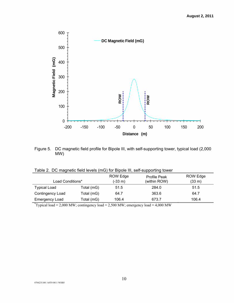
August 2, 2011
10 0704235.001 A0T0 0811 WHB5
Figure 5. DC magnetic field profile for Bipole III, with self-supporting tower, typical load (2,000 MW)
Table 2. DC magnetic field levels (mG) for Bipole III, self-supporting tower
Load Conditions* ROW Edge
(-33 m) Profile Peak (within ROW)
ROW Edge (33 m)
Typical Load Total (mG) 51.5 284.0 51.5
Contingency Load Total (mG) 64.7 363.6 64.7
Emergency Load Total (mG) 106.4 673.7 106.4 *Typical load = 2,000 MW; contingency load = 2,500 MW; emergency load = 4,000 MW
0
100
200
300
400
500
600
-200 -150 -100 -50 0 50 100 150 200
Mag
netic
Fie
ld (
mG
)
Distance (m)
DC Magnetic Field (mG)
RO
W
RO
W

August 2, 2011
11 0704235.001 A0T0 0811 WHB5
Figure 6. Example of total DC magnetic field (the earth’s geomagnetic field plus the DC magnetic field) for Bipole III, with self-supporting tower
Line orientation is north-south, and the cross-section view faces north. The dashed horizontal line indicates the level of the geomagnetic field alone.
0
100
200
300
400
500
600
700
800
900
1000
-200 -150 -100 -50 0 50 100 150 200
Mag
netic
Fie
ld (
mG
)
Distance (m)
DC Magnetic Field (mG)
RO
W
RO
W

August 2, 2011
12 0704235.001 A0T0 0811 WHB5
Figure 7. DC magnetic field profile for guyed tower Bipole I and Bipole II, typical loading
Table 3. DC magnetic field levels (mG) for Bipole I and Bipole II
Load Conditions* ROW Edge
(-55 m) Profile Peak (within ROW)
ROW Edge (55 m)
Typical Load Total (mG) 65.5 224.1 65.4 *Typical load – Bipole I = 1,559 MW; Bipole II = 1,681 MW
0
100
200
300
400
500
600
-200 -150 -100 -50 0 50 100 150 200
Mag
netic
Fie
ld (
mG
)
Distance (m)
DC Magnetic Field (mG)
RO
W
RO
W

August 2, 2011
13 0704235.001 A0T0 0811 WHB5
Electric fields
Figure 8. DC electric field profile for Bipole III, with guyed tower, typical loading (2,000 MW)
Table 4. DC electric field levels (kV/m) for Bipole III with guyed tower
Load Conditions* ROW Edge
(-33 m) Profile Peak (within ROW)
ROW Edge (33 m)
Typical Load Fair (kV/m) -4.3 -16.5 22.2 6.5
Foul (kV/m) -9.3 -29.8 29.8 9.3
Contingency Load Fair (kV/m) -4.3 -16.9 22.7 6.5
Foul (kV/m) -9.4 -30.5 30.5 9.4
Emergency Load Fair (kV/m) -4.3 -19.6 26.2 6.4
Foul (kV/m) -9.3 -34.9 34.9 9.3 *Typical load = 2,000 MW; contingency load = 2,500 MW; emergency load = 4,000 MW

August 2, 2011
14 0704235.001 A0T0 0811 WHB5
Figure 9. DC electric field profile for Bipole III, with self-supporting tower, typical loading (2,000 MW)
Table 5. DC electric field levels (kV/m) for Bipole III with self-supporting tower
Load Conditions* ROW Edge
(-33 m) Profile Peak (within ROW)
ROW Edge (33 m)
Typical Load Fair (kV/m) -4.4 -16.6 22.4 6.6
Foul (kV/m) -9.5 -30.1 30.1 9.5
Contingency Load Fair (kV/m) -4.4 -17.0 22.9 6.6
Foul (kV/m) -9.5 -30.8 30.8 9.5
Emergency Load Fair (kV/m) -4.3 -19.8 26.3 6.5
Foul (kV/m) -9.5 -35.1 35.1 9.5 *Typical load = 2,000 MW; contingency load = 2,500 MW; emergency load = 4,000 MW
-50
-40
-30
-20
-10
0
10
20
30
40
50
-200 -150 -100 -50 0 50 100 150 200
Ele
ctri
c Fi
eld
(kV
/m)
Distance (m)
Fair Weather DC Electric Field (kV/m)
Foul Weather DC Electric Field (kV/m)
RO
W
RO
W
Lattice

August 2, 2011
15 0704235.001 A0T0 0811 WHB5
Figure 10. DC electric field profile for Bipole I and II, with guyed tower, typical loading
Table 6. DC electric field levels (kV/m) for guyed tower Bipole I and II
Load Conditions* ROW Edge
(-55 m) Profile Peak (within ROW)
ROW Edge (55 m)
Typical Load Fair (kV/m) -7.6 -16.4 22.6 -8.9
Foul (kV/m) -14.4 -28.4 29.7 -16.4 *Typical load - Bipole I = 1,559 MW; Bipole II = 1,681 MW
-50
-40
-30
-20
-10
0
10
20
30
40
50
-200 -150 -100 -50 0 50 100 150 200
Ele
ctri
c Fi
eld
(kV
/m)
Distance (m)
Fair Weather DC Electric Field (kV/m)
Foul Weather DC Electric Field (kV/m)
RO
W
RO
W

August 2, 2011
16 0704235.001 A0T0 0811 WHB5
Audible noise
Figure 11. Median AN level in fair and foul weather for Bipole III with guyed tower, typical loading (2,000 MW)
The AN is referenced in dB above 20 Pa with an A-weighting level.
Table 7. Audible noise levels for Bipole III with guyed tower*
Load Conditions† ROW Edge
(-33 m) Profile Peak (within ROW)
ROW Edge (33 m)
Typical Load Fair (dB-A) 35.0 39.4 36.8
Foul (dB-A) 29.0 33.4 30.8
Contingency Load Fair (dB-A) 35.0 39.4 36.8
Foul (dB-A) 29.0 33.4 30.8
Emergency Load Fair (dB-A) 35.1 39.7 36.9
Foul (dB-A) 29.1 33.7 30.9 *275 m Altitude †Typical load = 2,000 MW; contingency load = 2,500 MW; emergency load = 4,000 MW

August 2, 2011
17 0704235.001 A0T0 0811 WHB5
Figure 12. Median AN level in fair and foul weather for Bipole III with self-supporting tower, typical loading (2,000 MW)
Table 8. Audible noise levels for Bipole III with self-supporting tower*
Load Conditions† ROW Edge
(-33 m) Profile Peak (within ROW)
ROW Edge (33 m)
Typical Load Fair (dB-A) 34.6 38.9 36.4
Foul (dB-A) 28.6 32.9 30.4
Contingency Load Fair (dB-A) 34.6 39.0 36.4
Foul (dB-A) 28.6 33.0 30.4
Emergency Load Fair (dB-A) 34.7 39.3 36.6
Foul (dB-A) 28.7 33.3 30.6 *275 m Altitude †Typical load = 2,000 MW; contingency load = 2,500 MW; emergency load = 4,000 MW

August 2, 2011
18 0704235.001 A0T0 0811 WHB5
Figure 13. Median AN level in fair and foul weather for Bipole I and II with guyed tower, typical loading
Table 9. Audible noise levels for guyed tower Bipole I and II*
Load Conditions† ROW Edge
(-55 m) Profile Peak (within ROW)
ROW Edge (55 m)
Typical Load Fair (dB-A) 47.2 50.1 45.7
Foul (dB-A) 41.2 44.1 39.7 *300 m Altitude †Typical load – Bipole I = 1,559 MW; Bipole II = 1,681 MW

August 2, 2011
19 0704235.001 A0T0 0811 WHB5
Radio noise
Figure 14. Median RN levels in fair and foul weather for Bipole III with guyed tower, typical
loading (2,000 MW)
Table 10. Radio noise levels for Bipole III with guyed tower*
Load Conditions† ROW Edge
(-33 m) Profile Peak (within ROW)
ROW Edge (33 m)
Typical Load Fair (dB-μV/m) 47.1 65.4 51.5
Foul (dB-μV/m) 41.1 59.4 45.5
Contingency Load Fair (dB-μV/m) 47.0 65.5 51.4
Foul (dB-μV/m) 41.0 59.5 45.4
Emergency Load Fair (dB-μV/m) 46.2 66.5 50.7
Foul (dB-μV/m) 40.2 60.5 44.7 *275m Altitude †Typical load = 2,000 MW; contingency load = 2,500 MW; emergency load = 4,000 MW

August 2, 2011
20 0704235.001 A0T0 0811 WHB5
Figure 15. Median RN levels in fair and foul weather for Bipole III with self-supporting tower, typical loading (2,000 MW)
Table 11. Radio noise levels for Bipole III with self-supporting tower*
Load Conditions† ROW Edge
(-33 m) Profile Peak (within ROW)
ROW Edge (33 m)
Typical Load Fair (dB-μV/m) 46.9 65.2 51.4
Foul (dB-μV/m) 40.9 59.2 45.4
Contingency Load Fair (dB-μV/m) 46.8 65.3 51.3
Foul (dB-μV/m) 40.8 59.3 45.3
Emergency Load Fair (dB-μV/m) 46.1 66.3 50.6
Foul (dB-μV/m) 40.1 60.3 44.6 *275m Altitude †Typical load = 2,000 MW; contingency load = 2,500 MW; emergency load = 4,000 MW

August 2, 2011
21 0704235.001 A0T0 0811 WHB5
Figure 16. Median RN levels in fair and foul weather for Bipole I and II with guyed tower, typical loading
Table 12. Radio noise levels for guyed tower Bipole I and II*
Load Conditions† ROW Edge
(-55 m) Profile Peak (within ROW)
ROW Edge (55 m)
Typical Load Fair (dB-μV/m) 60.7 71.9 58.7
Foul (dB-μV/m) 54.7 65.9 52.7 *300 m Altitude †Typical load – Bipole I = 1,559 MW; Bipole II = 1,681 MW

August 2, 2011
22 0704235.001 A0T0 0811 WHB5
Air ions
Figure 17. Profile of small ion density levels for Bipole III, with guyed tower, typical loading (2,000 MW)
Table 13. Small ion density levels for Bipole III with guyed tower
Load Conditions* ROW Edge
(-33 m) Profile Peak (within ROW)
ROW Edge (33 m)
Typical Load Fair (ions/cm3) -12,449 -68,548 97,145 16,008
Foul (ions/cm3) -18,194 -118,144 118,144 18,194
Contingency Load Fair (ions/cm3) -12,625 -70,675 100,283 16,195
Foul (ions/cm3) -18,382 -122,078 122,078 18,382
Emergency Load Fair (ions/cm3) -13,065 -87,602 124,810 16,606
Foul (ions/cm3) -18,764 -152,509 152,509 18,764 *Typical load = 2,000 MW; contingency load = 2,500 MW; emergency load = 4,000 MW
-175000
-125000
-75000
-25000
25000
75000
125000
175000
-200 -150 -100 -50 0 50 100 150 200
Ion
Den
sity
(ion
s/cm
3 )
Distance (m)
Fair Weather DC Ion DensityFoul Weather DC Ion Density
RO
W
RO
W

August 2, 2011
23 0704235.001 A0T0 0811 WHB5
Figure 18. Profile of small ion density levels for Bipole III with self-supporting tower, typical loading (2,000 MW)
Table 14. Small ion density levels for Bipole III with self-supporting tower
Load Conditions* ROW Edge
(-33 m) Profile Peak (within ROW)
ROW Edge (33 m)
Typical Load Fair (ions/cm3) -12,603 -68,044 97,174 16,310
Foul (ions/cm3) -18,589 -118,582 118,582 18,589
Contingency Load Fair (ions/cm3) -12,791 -70,112 100,254 16,510
Foul (ions/cm3) -18,791 -122,489 122,489 18,791
Emergency Load Fair (ions/cm3) -13,253 -87,158 124,982 16,945
Foul (ions/cm3) -19,198 -153,189 153,189 19,198 *Typical load = 2,000 MW; contingency load = 2,500 MW; emergency load = 4,000 MW
-175000
-125000
-75000
-25000
25000
75000
125000
175000
-200 -150 -100 -50 0 50 100 150 200
Ion
Den
sity
(ion
s/cm
3 )
Distance (m)
Fair Weather DC Ion DensityFoul Weather DC Ion Density
RO
W
RO
W

August 2, 2011
24 0704235.001 A0T0 0811 WHB5
Figure 19. Profile of small ion density levels for Bipole I and II, typical loading
Table 15. Small air ion levels for guyed tower Bipole I and II
Load Conditions* ROW Edge
(-55 m) Profile Peak (within ROW)
ROW Edge (55 m)
Typical Load Fair (ions/cm3) -25,658 -76,879 95,623 -28,828
Foul (ions/cm3) -35,496 -109,886 109,886 -38,694 *Typical load – Bipole I = 1,559 MW; Bipole II = 1,681 MW
-175000
-125000
-75000
-25000
25000
75000
125000
175000
-200 -150 -100 -50 0 50 100 150 200
Ion
Den
sity
(ion
s/cm
3 )
Distance (m)
Fair Weather DC Ion Density (ions/cc)Foul Weather DC Ion Density (ions/cc)

August 2, 2011
25 0704235.001 A0T0 0811 WHB5
Ion current density
Figure 20. Profile of ion current density for Bipole III with guyed tower, typical loading (2,000 MW)
Table 16. Ion current density for Bipole III with guyed tower
Load Conditions* ROW Edge
(-33 m) Profile Peak (within ROW)
ROW Edge (33 m)
Typical Load Fair (nA/m2) -1 -26 39 2
Foul (nA/m2) -4 -83 63 3
Contingency Load Fair (nA/m2) -1 -28 41 2
Foul (nA/m2) -4 -87 67 3
Emergency Load Fair (nA/m2) -1 -40 58 2
Foul (nA/m2) -4 -124 95 3 *Typical load = 2,000 MW; contingency load = 2,500 MW; emergency load = 4,000 MW
-100
-80
-60
-40
-20
0
20
40
60
80
100
-200 -150 -100 -50 0 50 100 150 200
Ion
Cur
rent
(n
A/m
2 )
Distance (m)
Fair Weather DC Ion Current
Foul Weather DC Ion Current
RO
W
RO
W
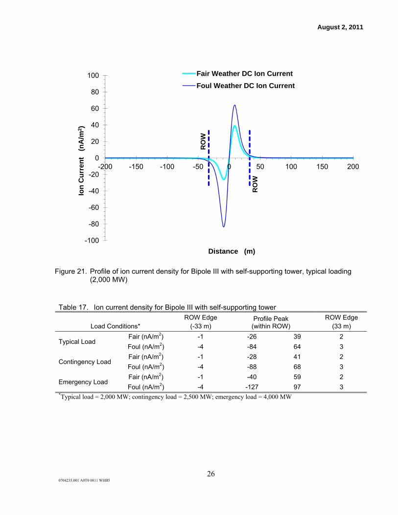
August 2, 2011
26 0704235.001 A0T0 0811 WHB5
Figure 21. Profile of ion current density for Bipole III with self-supporting tower, typical loading
(2,000 MW)
Table 17. Ion current density for Bipole III with self-supporting tower
Load Conditions* ROW Edge
(-33 m) Profile Peak (within ROW)
ROW Edge (33 m)
Typical Load Fair (nA/m2) -1 -26 39 2
Foul (nA/m2) -4 -84 64 3
Contingency Load Fair (nA/m2) -1 -28 41 2
Foul (nA/m2) -4 -88 68 3
Emergency Load Fair (nA/m2) -1 -40 59 2
Foul (nA/m2) -4 -127 97 3 *Typical load = 2,000 MW; contingency load = 2,500 MW; emergency load = 4,000 MW
-100
-80
-60
-40
-20
0
20
40
60
80
100
-200 -150 -100 -50 0 50 100 150 200
Ion
Cur
rent
(n
A/m
2 )
Distance (m)
Fair Weather DC Ion CurrentFoul Weather DC Ion Current
RO
W
RO
W

August 2, 2011
27 0704235.001 A0T0 0811 WHB5
Figure 22. Profile of ion current density for Bipole I and II, typical loading
Table 18. Ion current density levels for guyed tower Bipole I and II
Load Conditions* ROW Edge
(-55 m) Profile Peak (within ROW)
ROW Edge (55 m)
Typical Load Fair (nA/m2) -5 -30 39 -6
Foul (nA/m2) -12 -75 58 -15 *Typical load – Bipole I = 1,559 MW; Bipole II = 1,681 MW
-100
-80
-60
-40
-20
0
20
40
60
80
100
-200 -150 -100 -50 0 50 100 150 200
Ion
Den
sity
(nA
/m2 )
Distance (m)
Fair Weather DC Ion CurrentFoul Weather DC Ion Current
RO
W
RO
W

August 2, 2011
28 0704235.001 A0T0 0811 WHB5
Table 19. Comparison of the design and electrical characteristics of the proposed Bipole III line and existing overhead DC transmission lines
Transmission Line (kV)
Line Ht (m)
Pole Sep (m)
Cond. Bundle (mm)
Conductor Gradient (kV/cm)
Profile Peaks* Median Electric Field
(kV/m)/Median Small Ion (per cm3)
(-) Ion Current Density (nA/m2)
Fair Weather Foul Weather
Fair Weather
Foul Weather
Bipole III DC Line (Figure 1) [Self-supporting Tower] ±500 13.2 15.5 3x38 22.2 22 / 97,000 30 / 119,000
39 -84
Bipole III DC Line (Figure 2) [Guyed Tower] ±500 13.2 15.0 3x38 22.4 22 / 97,000 30 / 118,000
39 -83
Bipole I (Figure 3) ±463 13.5 13.4 2x41
25.5 23 / 96,000 30 /110,000 39 -75
Bipole II (Figure 3) ±500 13.5 27.0
DC Pacific Intertie-initial Oregon/California
±400 9.8 12.2 2x46 20.9 23 / 141,000 32 / 175,000 60 -135
CPA-UPA North Dakota ±400 10.7 12.2 2x38 24.1 23 / 125,000 30 / 148,000 53 -107
DC Pacific Intertie-upgrade Oregon/California ±500 9.8 12.2 2x46 26.1 34 / 199,000 45 / 231,000
125 -191
Intermountain Power Nevada
±500 12.2 12.8 3x39 20.5 22 / 105,000 30 / 135,000 43 -76
New Eng-Hydro Québec Vermont ±450 12.2 13.7 3x51 16.8 18 / 80,000 25 / 112,000
27 -67
*Electric fields rounded to the closest 10 kV/m and ion density rounded to the closest 100,000 ions/cm3

August 2, 2011
29 0704235.001 A0T0 0811 WHB5
4. Comparison of Bipole III and Bipole I/II Electrical Environments
It is difficult to succinctly compare the electrical environment of the proposed Bipole III line
with the Bipole I/II lines because of the large number of profiles and tables presented above.
Figure 23 compares the relative levels of electric field, magnetic field, air ions, ion current
density, AN, and RN on the ROW and at the edge of the ROW from these lines. Note that the
distance from the centerline of the Bipole III line to the ROW edges is 33 m, whereas the
distance from center line of the nearest Bipole I or II structure to the edge of the ROW is 22.5 m.
The peak values of calculated electric fields, air ions, and ion current density are very similar.
The peak magnetic field of Bipole I/II is lower because slightly lower typical loads (Bipole I =
1,559 MW; Bipole II = 1,681 MW) were assumed than were used for Bipole III (2,000 MW).
The peak values of AN and RN are lower on the ROW and at the edge of the ROW for Bipole III
than Bipoles I and II. This occurs largely because the surface gradient of the three-conductor
bundle of Bipole III is lower than the surface gradient of the two-conductor bundles of Bipole
I/II.

August 2, 2011
30 0704235.001 A0T0 0811 WHB5
Figure 23. Modeled electrical parameters at typical loading for Bipole III and Bipole I/II guyed tower configurations

August 2, 2011
31 0704235.001 A0T0 0811 WHB5
5. Ground Electrode/Electrode Line
The converter station is grounded by a low-voltage electrode line to a buried electrode. The
possibility of effects associated with the electric and magnetic fields from the electrode and the
electrode line are discussed below.
Ground Electrode
A remote ground electrode will be installed to correct small current imbalances between the
positive and negative conductors and during abnormal operating conditions. The electrode also
is expected to be used in a monopolar operating mode to maintain power transfer on an
emergency basis if a problem with a valve group or one of the conductor bundles is out of
service. Based on historical data on Bipoles I and II, a long-term outage rate of about 8% is
projected for one pole or the other due to maintenance or other outages. Most of the outages on
Bipoles I and II have involved valve groups or maintenance and the design of Bipole III allows
for such operations without the use of the ground electrode. Hence, the need for full power
return over the Bipole III electrode would be even less than for Bipoles I and II and would
primarily be limited to maintain power transfer only if the line conductors associated with the
outed pole were not available for use. The ground electrode is designed to operate at a
continuous current of 2,000 amperes (A) and at higher currents up to 2,750 A for a more limited
period. The ground potential rise (GPR) at the neutral bus in the converter terminals will be low
under all operating conditions; however, DC characteristic and non-characteristic harmonic
current flows through the neutral conductors must also be considered. Thus, for touch and step
potential considerations, the neutral bus must be classified as a high voltage conductor.
The electrode, as planned, is a ring electrode with a diameter between 350 and 650 m (the exact
diameter will depend on the final design). The ring will be fed from a power pole placed in the
center of the ring at which the electrode line will be terminated as shown in Figure 24. Four
cable circuits will be placed with 90 degree separations to connect the electrode line to the ring
electrode. Disconnect switches will be placed on the pole used for the line termination to enable
interruption of the current flowing to segments of the ring.
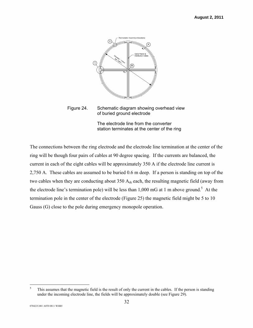
August 2, 2011
32 0704235.001 A0T0 0811 WHB5
Figure 24. Schematic diagram showing overhead view of buried ground electrode
The electrode line from the converter station terminates at the center of the ring
The connections between the ring electrode and the electrode line termination at the center of the
ring will be though four pairs of cables at 90 degree spacing. If the currents are balanced, the
current in each of the eight cables will be approximately 350 A if the electrode line current is
2,750 A. These cables are assumed to be buried 0.6 m deep. If a person is standing on top of the
two cables when they are conducting about 350 Adc each, the resulting magnetic field (away from
the electrode line’s termination pole) will be less than 1,000 mG at 1 m above ground.5 At the
termination pole in the center of the electrode (Figure 25) the magnetic field might be 5 to 10
Gauss (G) close to the pole during emergency monopole operation.
5 This assumes that the magnetic field is the result of only the current in the cables. If the person is standing
under the incoming electrode line, the fields will be approximately double (see Figure 29).

August 2, 2011
33 0704235.001 A0T0 0811 WHB5
Figure 25. Termination of the electrode line at pole at the center of the ring electrode and transition to underground cable
The magnetic fields to which a person would be exposed standing on top of the electrode ring
will depend on where the person is standing along the periphery of the ring. The current flowing
from the electrode into the ground can be assumed to be uniformly distributed with vertical and
tangential (horizontal) current components. The currents flowing in the cables that form the
contact between the electrode material and the conductor imbedded in the electrode will have a
maximum level close to the electrode infeed (contact) points and the currents flowing in the
electrode cables will be concentrated in the insulated cables. Although closed form solutions for
calculating the fields can be used (Uhlmann, 1975), a numerical solution would be most useful
for mapping the fields. The fields should be lower at all points within the electrode area,
however, than the fields directly above the electrode cables discussed above. The far-fields some
distance away from the ground electrodes will depend on the local geology, and to calculate
these fields would require a detailed map of the soil resistivity.
The step potentials to which personnel will be exposed when walking across the electrode sites
during emergency operation have been calculated (Teshmont, 2010; 2011). The step potentials
are between approximately 5 volts/metre (V/m) and 10 V/m. The calculations have been made
assuming normal soils without any consideration for soil resistivity variations as a function of
season. The type of soil and the resistivity of the soil have a significant influence on the step

August 2, 2011
34 0704235.001 A0T0 0811 WHB5
potential. The resistivity is strongly correlated with the moisture content and temperature of the
soil (Morgan, 1993). Frozen soils have very high resistivity, which should tend to increase the
resistance of the electrode by reducing the volume of low resistance soil surrounding the
electrode material. Thus, the resistivity of soils is a highly complex issue but of significant
importance when assessing safety issues. Therefore, even though the electrodes themselves are
intended to be installed below the frost zone, the current distribution around the electrodes can be
affected if the soil is frozen. Since the resistivity can be an order of magnitude or higher if the
soil is frozen, a calculation assuming frozen soil should be performed during final design.6
The step potentials have been calculated assuming steady-state current flow into the electrode
during monopolar operation.7 This is for the most part conservative. When a short circuit from a
pole to ground occurs, however, the current can increase to two or three times the normal
current. The instantaneous current change is limited by the pole to ground surge impedance,
which means that the current will rise by about 1.5 kiloampere (kA) on the faulted conductor.
This current will flow through the electrode line to the converter station. The current control
system in the rectifier station should limit the overcurrent, but the actual peak current and the
duration of this peak current depends on the speed of response of the control system. That is, the
electrode current could change by about 3 to 4 kA. During the interval when the failed pole is
de-energized to enable clearing of the fault, the other pole will operate with full current through
the electrode. Upon restart of the faulted pole and assuming that the fault is cleared, normal
bipolar operation will be resumed with low or insignificant electrode current flow. The peak
fault current might last for 20 to 50 milliseconds. That is sufficiently long to have an effect on
the step potentials to which people or animals might be exposed. Therefore, the step potentials
should also be calculated for fault conditions.
6 When the temperature is below freezing, water injection into the soil is probably not practical. Replenishing the
water around the electrodes under these conditions, however, might be warranted since the soil around the electrode will not be wetted by rain water for as long as the soil remains frozen.
7 No touch potentials have been calculated. If the electrode is conducting current and if someone drives a vehicle or some machinery out over the electrodes, however, a person contacting the truck or machinery will be exposed to touch potentials that could be significantly higher than the step potentials under similar conditions. The risks associated with touching conducting objects on the electrode sites should, therefore, be assessed.

August 2, 2011
35 0704235.001 A0T0 0811 WHB5
Injection of 60-Hz currents from a converter should also be considered. This can happen as a
result of commutation failures in the inverter end of the line or as a result of valve misfires.
These alternating current (AC) injections will probably have less effect on the electrode current
flows than a pole to ground fault although commutation failures are associated with overcurrents
and also at times lead to current zeros in the line current of the affected pole. In that case, the
direct current will go to zero and the system will recover from this condition after some time.
Drying out of the electrodes could lead to a thermal run-away of the electrodes. This could in
theory lead to overheating and even pyrolysis (thermal degradation) of the coke typically used
around the electrodes. The resistance of the electrode would, however, have to increase
significantly prior to electrode dry-out. Therefore, it should be possible to detect the increasing
electrode resistance prior to the thermal runaway by monitoring the GPR between the electrode
line and the station ground mat. The best remedy to avoid dry-out of the electrodes is to keep the
electrodes wet, although this might not be easy to do during winter conditions with frozen soils.
Step potentials for most animals walking across the electrode site will be even lower than for a
person because of their shorter strides, but for large animals, such as a moose at stand-still, the
step potentials could be two to three times higher than for people. However, at the same time,
the recommended limits for large animals are more than twice those for people (IEC, 2007).
A small stream is about 800 m from the northern boundary of the site for the ground electrode.
The potential experienced by fish in this stream during operation of the ground electrode was
estimated. The site for the ground electrode is a square plot of land approximately 1.6 km on
each side. To simplify the computations, the ground electrode was assumed to be located at the
center of this square. It was also assumed that no current flows inwards towards the center of the
electrode area. End effects were ignored by assuming that the electrode extends infinitely in
length with a uniform current density to a depth equivalent to the distance of the stream from the
nearest edge of the ground electrode ring. In the absence of detailed information, the soil was
assumed to be uniform at least up to a depth also equivalent to the distance of the stream from
the nearest edge of the ground electrode ring. The electric field experienced by a fish in a
shallow stream 800 m from the edge of the ground electrode site (1.6 km x 1.6 km) with a buried
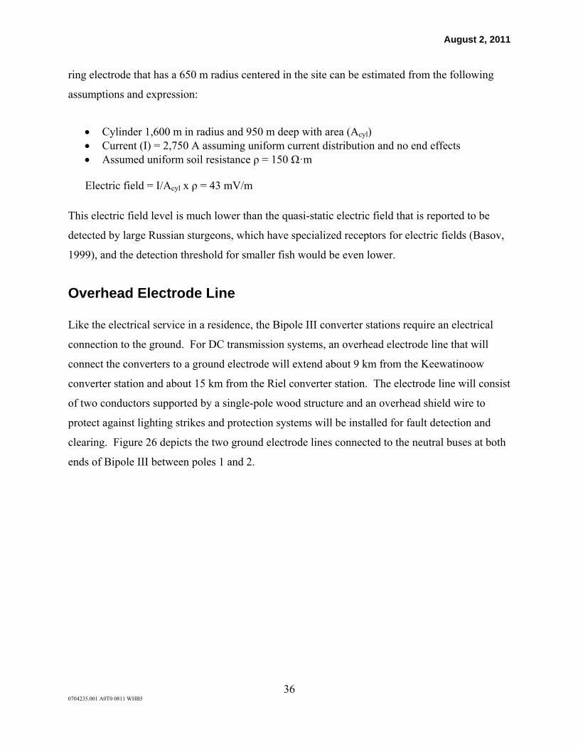
August 2, 2011
36 0704235.001 A0T0 0811 WHB5
ring electrode that has a 650 m radius centered in the site can be estimated from the following
assumptions and expression:
Cylinder 1,600 m in radius and 950 m deep with area (Acyl) Current (I) = 2,750 A assuming uniform current distribution and no end effects Assumed uniform soil resistance ρ = 150 Ω·m
Electric field = I/Acyl x ρ = 43 mV/m
This electric field level is much lower than the quasi-static electric field that is reported to be
detected by large Russian sturgeons, which have specialized receptors for electric fields (Basov,
1999), and the detection threshold for smaller fish would be even lower.
Overhead Electrode Line
Like the electrical service in a residence, the Bipole III converter stations require an electrical
connection to the ground. For DC transmission systems, an overhead electrode line that will
connect the converters to a ground electrode will extend about 9 km from the Keewatinoow
converter station and about 15 km from the Riel converter station. The electrode line will consist
of two conductors supported by a single-pole wood structure and an overhead shield wire to
protect against lighting strikes and protection systems will be installed for fault detection and
clearing. Figure 26 depicts the two ground electrode lines connected to the neutral buses at both
ends of Bipole III between poles 1 and 2.
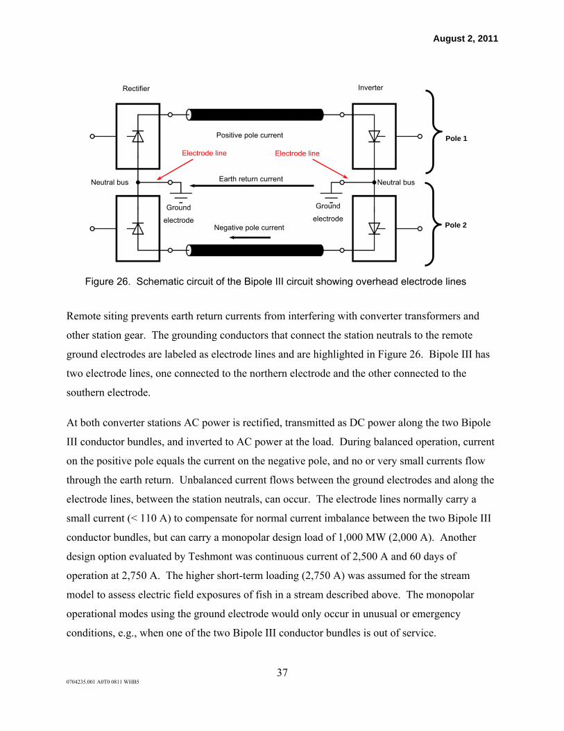
August 2, 2011
37 0704235.001 A0T0 0811 WHB5
Figure 26. Schematic circuit of the Bipole III circuit showing overhead electrode lines
Remote siting prevents earth return currents from interfering with converter transformers and
other station gear. The grounding conductors that connect the station neutrals to the remote
ground electrodes are labeled as electrode lines and are highlighted in Figure 26. Bipole III has
two electrode lines, one connected to the northern electrode and the other connected to the
southern electrode.
At both converter stations AC power is rectified, transmitted as DC power along the two Bipole
III conductor bundles, and inverted to AC power at the load. During balanced operation, current
on the positive pole equals the current on the negative pole, and no or very small currents flow
through the earth return. Unbalanced current flows between the ground electrodes and along the
electrode lines, between the station neutrals, can occur. The electrode lines normally carry a
small current (< 110 A) to compensate for normal current imbalance between the two Bipole III
conductor bundles, but can carry a monopolar design load of 1,000 MW (2,000 A). Another
design option evaluated by Teshmont was continuous current of 2,500 A and 60 days of
operation at 2,750 A. The higher short-term loading (2,750 A) was assumed for the stream
model to assess electric field exposures of fish in a stream described above. The monopolar
operational modes using the ground electrode would only occur in unusual or emergency
conditions, e.g., when one of the two Bipole III conductor bundles is out of service.
Ground
electrode
Ground
electrode
Inverter Rectifier
Positive pole current
Earth return current
Negative pole current
Pole 1
Pole 2
Electrode line Electrode line
Neutral bus Neutral bus

August 2, 2011
38 0704235.001 A0T0 0811 WHB5
The northern and southern electrode lines are similar in appearance to an ordinary low-voltage
AC distribution line, as shown in the representative design in Figure 27. At tangent locations,
the electrode lines will be supported on 40-50 foot wood poles carrying two conductors each 1-
inch in diameter.
Figure 27. Representative design of the structure of the north and south electrode lines
During bipole operation, the electrode lines will produce electric or magnetic fields far smaller
than those in the vicinity of the Bipole III conductors. The total magnetic field around the
electrode line during normal bipole operation, including the effect of the geomagnetic field is
depicted in Figure 28.
2.13 m separation
height
6.71 m
sag sag
height
6.71 m
sag
height
6.71 m
2.13 m separation
sag
height
6.71 m

August 2, 2011
39 0704235.001 A0T0 0811 WHB5
Figure 28. Total DC magnetic field (geomagnetic+electrode line) during bipolar operation of the Bipole III transmission line
In the depicted profile, the electrode line is oriented north-south and carries southbound current (110 A). The dashed line indicates the level of the geomagnetic field alone.
Calculated magnetic fields for other directions of current flow are summarized in Tables 20 and 21.

August 2, 2011
40 0704235.001 A0T0 0811 WHB5
Table 20. Deviation of total DC magnetic field (cables + geomagnetic) from 577 mG, for north-south orientation of electrode line
Operating condition Current direction
Offset from centerline*
-100 m -50 m max +
deviation max –
deviation +50 m +100 m
bipole north -2.1 -4.2 18.3 -18.3 4.2 2.1
south 2.1 4.2 18.9 -17.7 -4.2 -2.1
monopole (emergency)
north -48.1 -94.9 555.5 -272.2 95.9 48.3
south 48.4 96.2 566.5 -262.4 -94.5 -48.0
*Positions are reported for view facing north (-west +east)
Table 21. Deviation of total DC magnetic field (cables + geomagnetic) from 577 mG, for east-west orientation of electrode line
Operating condition Current direction
Offset from centerline*
-100 m -50 m max +
deviation max –
deviation +50 m +100 m
bipole east -2.1 -4.1 23.9 -13.9 4.3 2.2
west 2.1 4.1 14.4 -23.4 -4.3 -2.2
monopole (emergency)
east -47.2 -91.2 646.3 -205.6 98.5 49.0
west 47.6 93.6 474.7 -382.5 -98.1 -48.8
*Positions are reported for view facing east (-north +south)
When needed in an emergency, monopole operating current will flow on the electrode lines and
change the existing magnetic field near the line as shown in Figure 29. In any condition, the
calculated electric field 1 m above ground is below 0.7 kV/m at a 7.5 kV potential (the maximum
anticipated potential) as shown in Figure 30. The ground electrode line will not be a significant
source of corona-generated AN or RN because of its low voltage.

August 2, 2011
41 0704235.001 A0T0 0811 WHB5
Figure 29. Total DC magnetic field (geomagnetic+electrode line) during emergency monopolar operation of the Bipole III transmission line
In the depicted profile, the electrode line is oriented north-south and carries southbound current (2,500 A). The dashed line indicates the level of the geomagnetic field alone.

August 2, 2011
42 0704235.001 A0T0 0811 WHB5
Figure 30. Calculated DC electric field profile for the electrode line at 7.5 kV potential
AC Harmonic currents
A DC bipole consists of a number of 6-pulse converter groups connected in series as shown in
simplified form in Figure 31. The electrode lines are typically brought out from the terminals to
a remote location where the land electrodes are located to avoid injecting DC currents into the
converter stations’ ground grid.

August 2, 2011
43 0704235.001 A0T0 0811 WHB5
Figure 31. DC Bipole configuration showing 6-pulse converter groups and electrode lines
If two 6-pulse groups are connected in series as shown in Figure 32, and one is fed from a Y-Y
connected transformer and the other via a Y-Delta connected transformer, the output voltage
from the converter will mainly contain 12-pulse harmonics and multiples thereof (Reeve and
Baron, 1970; Lasseter et al., 1977; Mathur and Sharaf, 1983). These are the so-called
“characteristic harmonic voltages.” The harmonic voltages generated in these converters are
partially blocked by a smoothing reactor normally placed between the converter groups and the
DC line conductors. Harmonic filters, which further attenuate the harmonic voltages, are
typically installed to filter out these harmonics from the DC voltage as it enters the line as shown
in Figure 33 (Adamson et al., 1983; Garrity et al., 1989). Improved filtering can also be
achieved by using active filtering systems (Zhang et al., 1993). It is important that the DC filters
are connected to the neutral bus, otherwise the harmonic currents would flow back to the
converter station through the electrode line. It is also important that the neutral bus is protected
against overvoltages delivered to the station from the line and conducted through the filters to the
low voltage neutral bus. An arrester, possibly in parallel with a surge capacitor (as shown in
Figure 33), therefore, is often used for overvoltage protection of the neutral bus.
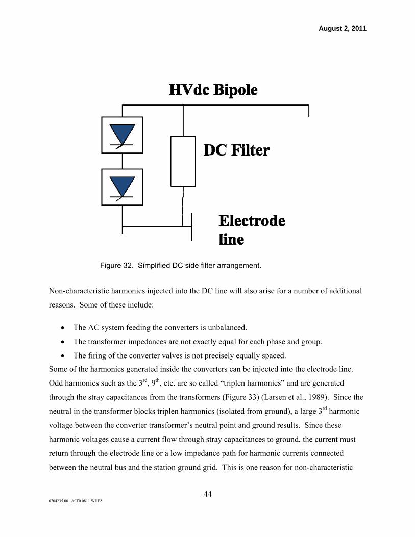
August 2, 2011
44 0704235.001 A0T0 0811 WHB5
Figure 32. Simplified DC side filter arrangement.
Non-characteristic harmonics injected into the DC line will also arise for a number of additional
reasons. Some of these include:
The AC system feeding the converters is unbalanced.
The transformer impedances are not exactly equal for each phase and group.
The firing of the converter valves is not precisely equally spaced.
Some of the harmonics generated inside the converters can be injected into the electrode line.
Odd harmonics such as the 3rd, 9th, etc. are so called “triplen harmonics” and are generated
through the stray capacitances from the transformers (Figure 33) (Larsen et al., 1989). Since the
neutral in the transformer blocks triplen harmonics (isolated from ground), a large 3rd harmonic
voltage between the converter transformer’s neutral point and ground results. Since these
harmonic voltages cause a current flow through stray capacitances to ground, the current must
return through the electrode line or a low impedance path for harmonic currents connected
between the neutral bus and the station ground grid. This is one reason for non-characteristic

August 2, 2011
45 0704235.001 A0T0 0811 WHB5
harmonic current flows on electrode lines.8 Although small, such harmonic current flows might
cause telephone interference depending on the magnitude of harmonic currents and the proximity
and parallel length of telephone lines. Since the 3rd harmonic at 180 Hz is below the lower
threshold of a telephone channel at 300 Hz and the 9th harmonic at 540 Hz is towards the lower
end of the typical 4 kHz bandwidth for a voice grade channel, the interference factor is probably
below the threshold where it will be noticeable by telephone users unless the electrode line
happens to be tuned to one of the non-characteristic harmonics9. One factor to consider is that
these harmonic currents are not related to the DC line current but arise as a result of the
commutation voltages in the converter groups. That is, they could have a higher magnitude at
low operating power levels than at high operating power levels.
Figure 33. Stray capacitance from the transformers to ground.
Commutation voltage transients will also cause current flow through stray capacitances from
valves, bushings, and bus structures to ground. If there are high frequency blocking filters
inserted between the lower voltage converter group and the neutral bus, these transients should
not propagate along the electrode line. If not, there is the possibility for interference with
8 If the smoothing reactor is placed at the neutral end of the converter groups, then the triplen harmonics will
enter the DC pole conductor instead of the electrode line. 9 The electrode line at the Celilo converter station of the Pacific Intertie transmission line was tuned to the 6th
harmonic, which caused some telephone interference.

August 2, 2011
46 0704235.001 A0T0 0811 WHB5
systems operating in the kHz to hundreds of kHz range. That is, there is a possibility for radio
and carrier communication system interference as a result of conducted transients injected into
the electrode line even if the line does not have corona discharges.
Electric and magnetic fields from the electrode line
As can be seen in Figure 34, the DC filter creates a path for transients to enter the neutral bus
when connected to this bus. If the filter is connected to the station ground, then the harmonics
generated in the converter groups will have to go through the electrode line in order to return to
their source in the converters unless there is a low impedance path for the harmonics from the
station ground mat to the neutral bus. A capacitor connected from the neutral bus to ground can
serve as a low impedance path for harmonics. (Such a capacitor will also allow triplen
harmonics discussed above to return to the converter where they were generated.)
The electrode line can also conduct lightning surges into the station, requiring a surge arrester
connected between the neutral bus and station ground as shown in Figure 34. This limits the
electric fields at the point at which the arrester is connected to the neutral bus to the protection
level of the arrester. That is, the voltage at the station end of the electrode line will be at or
below the voltage at which the arrester conducts current.
Lightning striking the electrode line will cause line overvoltage, potentially to the point causing a
flashover (an arc) across a line insulator. Such faults are difficult to detect and are also difficult
to isolate to allow the line insulation to recover. In at least one monopole DC line project a
sufficient number of insulators were installed for the electrode line to enable the DC current flow
through the fault to extinguish by itself. In a bipolar system such as the Bipole III line, the
current in the electrode line will normally be very low and a fault current from the electrode line
to ground would most likely extinguish by itself. If the electrode is carrying 2,750 A, however,
the arc voltage generated at the fault location from the magnetic forces that cause the arc to
become elongated might not be sufficient to extinguish the arc unless the air gap is large.10 The
air gap or the required insulator length would most likely have to be longer closer to the
10 The emergency rating of the electrode line should be used when selecting the appropriate number of insulators
to use for the line.

August 2, 2011
47 0704235.001 A0T0 0811 WHB5
converter station as opposed to closer to the electrode site to accomplish natural commutation of
the fault current back into the electrode line conductor.
Figure 34. Common neutral bus overvoltage protection and bus capacitor.

August 2, 2011
48 0704235.001 A0T0 0811 WHB5
6. Converter Station
Converter stations will be connected to each end of the Bipole III line to transfer AC to DC
power at the northern converter and DC to AC power at the southern converter. In addition there
will be associated equipment and facilities to connect to AC transmission lines and switching
facilities.
The electric and magnetic fields associated with equipment in the converter station would not be
expected to cause field levels outside the boundaries of the large proposed sites to be
significantly elevated except where power lines, e.g., Bipole III, or connections to the AC grid
traverse the boundary. The field levels associated with the operation of Bipole III have been
characterized above in Section 3.
As discussed in Section 4, however, the output voltage from the converter will mainly contain
12-pulse harmonics and multiples thereof and can be a potential source of conducted as well as
radiated interference at frequencies above the telephone interference spectrum. The
commutation of the valve currents from one valve to the adjacent valve is associated with short
duration short circuits between the AC phase voltages. These switching transients also cause
charging and discharging currents to flow through stray capacitances from the equipment to
ground or between equipment connected to difference phases. The commutation leads to one
transient voltage change when a valve is turned on and another when the valve is turned off.
Thus, in a 6-pulse group connected to a 60-Hz system, there will be two sets of transients with a
360-Hz repetition frequency.
The RN levels from thyristor switched valves depend on a number of factors. The turn-on speed
of the thyristors is one of these factors (Temple, 1981). A slower turn-on speed tends to reduce
the higher frequencies in the RN spectrum but at the expense of higher switching losses. The
valve halls are typically built as shielded rooms to prevent significant RN from the valve
switching. Some relatively low-level high-frequency currents, however, may escape the building
via the converter transformers and DC bus connections to the smoothing reactors and the
electrode line (EPRI, 1986). Although the impedance of a transformer might be viewed as an

August 2, 2011
49 0704235.001 A0T0 0811 WHB5
inductance for power system frequencies, the high frequency impedance of a transformer is
complex and appears as a series capacitance or as a series resonant circuit with hardly any
attenuation for some frequencies. Similarly, a capacitor might be represented by an inductance
at some higher frequencies. Therefore, special RF blocking filters are sometimes installed in the
AC and DC busses in the valve hall to reduce the RF noise levels outside the converter station.
The switching-related current impulses injected into the busses leaving the valve hall causes RF
energy to be radiated from the AC and DC busses, but the impulse currents can also cause
interference with carrier communication systems (Hylten-Cavallius et al., 1964; Annestrand,
1972; Patterson, 1985; Maruvada et al., 1989; EPRI, 1994) . The interference levels are
typically worse for AM communication systems. Thus, in addition to carrier communications
system interference, long wave through short wave AM radio systems can be affected. Thus,
most of the RN frequencies of concern are below 1 megahertz (MHz). FM systems are typically
not affected by the valve switching.
Assuming standard design practices to minimize RF interference from the converter station and
electrode line, harmonics and RF are not likely to be a problem, and if interference is detected, it
will be mitigated.

August 2, 2011
50 0704235.001 A0T0 0811 WHB5
7. Assessment Criteria and Conclusions
DC fields and ions
For DC electric and magnetic fields, two organizations have developed guidance. The
International Commission on Non-Ionizing Radiation Protection (ICNIRP) recently published
guidelines on exposure to DC magnetic fields that included a limit for exposure of the general
public of 400 millitesla (mT), which is equivalent to 4,000,000 mG (ICNIRP, 2009). The
magnetic field contributed by the line in normal operation to the background geomagnetic field is
a very, very small fraction of this limit; on the ROW the magnetic field contributed by the line is
less than 360 mG. Higher magnetic fields will occur during some infrequent emergency ground
return operating modes.
The National Radiological Protection Board of Great Britain (NRPB), now a division within the
Health Protection Agency of Great Britain, has recommended 25 kV/m as the limit on the
exposure of the general public to DC electric fields (NRPB, 1994). A similar value has been
recommended as a threshold limit value for occupational exposures (ACGIH, 2009). A higher
value of 42 kV/m was recommended as an upper limit (basic restriction) in a Comité Européen
de Normalisation Électrotechnique pre-standard (CENELEC, 1995). In fair weather, the
calculated DC electric fields of Bipole III are below 25 kV/m. In foul weather, in which persons
are less likely to be on the ROW, the DC electric fields are expected to exceed this value within
the ROW for about 10 m on either side of Bipole III for no-wind conditions.
No scientific or regulatory agency has determined that small air ions, a measure of air ions and
electric fields together (ion current density) pose a threat to the environment or health, so no
exposure guidelines have been proposed. Small air ions are found at varying levels in the
everyday environment. Since low levels of air ions in buildings have been alleged as
symptomatic of poor indoor air quality, the Ministry of Health of the Russian Federation has
recommended that (+) and (-) air ion levels be maintained between a minimum level of 400
ions/cm3 and a maximum level of 50,000 ions/cm3 for public and industrial quarters (MHRF,
2003). The basis for the guideline was not described in this hygienic norm. The levels of air

August 2, 2011
51 0704235.001 A0T0 0811 WHB5
ions on the ROW exceed this range but fall well within this range outside the ROW and are
similar to those found in environments not near a DC transmission line.
DC audible noise
Manitoba’s Provincial Guidelines specify maximum desirable 1-hour equivalent noise levels for
residential and commercial areas of 55 d-BA and 45 d-BA, for day-time and night-time periods,
respectively (EMD, 1992). These standards will be met by Bipole III in fair weather even under
the conductors on the ROW. In foul weather, the levels of AN will be even lower and typically
masked by noise from wind and rain.
DC radio noise
The Industry Canada standard for RN for a 500-kV transmission line is 60 dBV/m at 15 m from
the nearest conductor that would be measured by a CISPR-type measuring instrument according
to CSA Standard C108.1.1-1977 (Industry Canada, 2001). This standard will be met by Bipole
III at the edges of the ROW and beyond in fair weather; in foul weather the levels will be even
lower.
Ground electrode/electrode line
In normal operation the ground electrode and electrode line will be associated with very weak
electric and magnetic fields. During monopolar operation with ground return the magnetic field
and electric fields will increase but still will be far below recommended limits discussed above.
The voltages on the electrode line will be too low to be a cause of corona-related AN or RN.
The ground electrode is designed to operate at a continuous current of 2,000 A and a higher
current of 2,500 A for a more limited period of time. Step potentials have been estimated to be
less than 10 V/m at 2,250 A and thus should not pose a hazard to humans and animals on the site
or to fish in a stream 800 m distant.
There will be no effects on the operation of communication equipment or radio/TV reception due
to the low operating voltage of the electrode line and the electrode. The physical presence of the

August 2, 2011
52 0704235.001 A0T0 0811 WHB5
conductors and tower structures may cause scattering, reflection, or reradiation of primary TV
broadcast signals. TV and RN interference may result from gap sparking caused by faulty or
loose fittings; such situations are easily remedied by routine maintenance. Although harmonic
voltages and currents on the electrode line can sometimes be a source of interference to
telephone communication, it can be mitigated.
Conclusions
Based on the modeling of the DC Bipole III transmission line and the ground electrode lines, the
following conclusions were drawn:
The small differences in conductor size and spacing between the guyed and self-
supporting Bipole III tower structures result in negligible differences in the levels of
calculated electric parameters.
In general, the calculated peak levels of AN and RN under Bipole III are substantially
lower than under Bipoles I and II and the levels of electric field, air ions, and ion currents
are similar. Only the peak magnetic field under the Bipole III line is higher and this is
because it was modeled at higher loading than Bipoles I and II. Bipole III was designed
to operate at the same loading as Bipole II.
During rare periods of monopolar operation, the levels of DC electric fields, air ions, and
ion current density will increase slightly (~10%) on the ROW and the edge of the ROW
closest to the operating pole compared to bipolar operation; levels are decreased by a
larger percentage at the edge of the ROW closest to the inactive pole. In contrast, AN
and RN levels decrease across the ROW, particularly during monopolar negative pole
operation.
At ground electrode sites, the levels of DC electric and magnetic fields will be very low
but will increase substantially above the buried electrode and beneath the electrode lines
during some rare emergency monopolar operations. The electrode is designed to keep the
step potentials low during monopolar operation so as to prevent shocks to persons or

August 2, 2011
53 0704235.001 A0T0 0811 WHB5
animals on the site and beyond. AC harmonics on the electrode line and RF noise from
the converter station are a possible source of interference to telephone communication
and AM radio reception but can be mitigated.
The levels of magnetic fields, electric fields, AN, RN, and small air ions outside the
ROW of Bipole III are all below limits recommended by provincial, national, and
international agencies. No guidance for the ion current density was identified but
compliance of Bipole III with both electric field and small air ion recommended limits
indicates that this parameter, computed as the product of the electric field and small ion
concentration, is not of additional consequence.
A comparison between Bipole III and six other DC transmission lines in North America
shows that the median peak levels of DC electric field and small air ions of Bipole III are
lower than the levels of five other DC transmission lines.

August 2, 2011
54 0704235.001 A0T0 0811 WHB5
References
Adamson KA, Lasseter RA, Melvold DJ, Reavis MA. DC side filtering studies for Pacific HVDC Intertie voltage upgrading. IEEE Transactions on Power Apparatus and Systems PAS-102, 1983.
American Conference of Governmental Industrial Hygienists (ACGIH). Documentation of the Threshold Limit Values for Physical Agents. Cincinnati, OH: ACGIH, 7th Edition, 2009.
Annestrand SA , Radio Interference from HVdc Converter Stations, IEEE Transactions on Power Apparatus and Systems. 91: 874 – 882, 1972.
Basov BM. Behavior of Sterlet Acipenser ruthenus and Russian Sturgeon A. gueldenstaedtii in low-frequency electric fields. Journal of Ichthyology 39: 782-787, 1999.
Canadian Standards Association (CSA). Electromagnetic Interference Measuring Instrument – CISPR Type. Standard C108.1.1-1977, Reaffirmed 2008.
Comité Européen de Normalisation Électrotechnique (CENELEC). Human Exposure to Electromagnetic fields low-frequency (0 Hz to 10 kHz). ENV 50166-1, 1995.
Environmental Management Division, Province of Manitoba Enforcement (EMD). Guidelines for Sound Pollution. September 21, 1992.
EPRI. Radio Interference From HVDC Converter Stations - Modeling and Characterization, EPRI report EPRl EL-4956, Project 1769-1 Final Report, December, 1986.
EPRI. High-Voltage Direct Current Handbook, First Edition, Chapter 15, AC Filter Design, EPRI report TR-104166, 1994.
Garrity TF, Hassan ID, Adamson KA, Donahue JA. Measurement of harmonic currents and evaluation of the DC filter performance of the New England-Hydro-Quebec Phase 1 HVDC project. IEEE Transactions on Power Delivery 4, Jan. 1989.
Hylten-Cavallius N, Annestrand S, Witt H, Madzarevic, V. Power Apparatus and Systems, IEEE Transactions on. 83:500 – 508, 1964.
International Electrotechnical Commission (IEC). General Guidelines for the Design of Ground Electrodes for High-Voltage Direct Current (HVDC) Links. IEC PAS 62344 Pre-Standard, First Edition, 2007-05, 2007.
Industry Canada. Spectrum Management and Telecommunications Policy, Interference-Causing Equipment Standard. Alternating Current High Voltage Power Systems. ICES-004, Issue 3, December, 2001.
International Commission on Non-Ionizing Radiation Protection (ICNIRP). Guidelines on limits of exposure to static magnetic fields. Health Physics 96:504-514. 2009.

August 2, 2011
55 0704235.001 A0T0 0811 WHB5
Institute of Electrical and Electronics Engineers (IEEE). IEEE recommended practice for instrumentation: specifications for magnetic flux density and electric field strength meters-10 Hz to 3 kHz. IEEE Standard 1308-1994, 1994.
Larsen EV, Sublich M, Kapoor SC. Impact of stray capacitance in HVDC harmonics. IEEE Transactions on Power Delivery 4(1), Jan. 1989.
Lasseter RH, Kelley FW, Lindh CB. DC filter design methods for HVDC systems. IEEE Transactions on Power Apparatus and Systems, PAS-96, Mar/Apr 1977.
Maruvada PS, Malewski R, Wong PS. Measurement of the electromagnetic environment of HVdc Converter Stations. IEEE Transactions on Power Delivery. 4: 1989.
Mathur RM and Sharaf AM. Harmonics on the DC side in HVDC conversion. IEEE Transactions on Power Apparatus and Systems, PAS-96(5), Sep/Oct 1977.
Ministry of Health of Russian Federation (MHRF). SanPin (Sanitary and Epidemiological Norms) 2.2.4. 1294-03 (New SanPin), June 16, 2003. http://www.ionization.info/issue/iss6.htm.
Morgan J. Cathodic Protection. In Cathodic Protection Criteria, 2nd Ed., pp. 67 –70. National Association of Corrosion Engineers, 1993.
National Radiological Protection Board (NRPB). Electromagnetic fields and the risk of cancer. Supplementary report by the Advisory Group on Non-ionizing Radiation. National Radiological Protection Board. 5(2):77-81, 1994.
National Geophysical Data Center (NGDC). 2010. Compute Earth's Magnetic Field Values. Internet website: http://www.ngdc.noaa.gov/geomag/magfield.shtml . Accessed: April, 2010.
Patterson NA. Carrier Frequency interference from HVdc systems., IEEE Transactions on Power Apparatus and Systems. PAS-104: 1985.
Reeve J and Baron JA. Harmonic DC line voltages arising from HVDC power conversion. IEEE Transactions on Power Apparatus and Systems. PAS-89(7), Sep/Oct 1970.
Temple VAK. Comparison of light triggered and electrically triggered thyristor turn-on, IEEE Transactions on Electron Devices .28:860-865, 1981.
Teshmont Consultants LP. Site Selection and Design of Bipole III DC Land Electrodes: North Electrode Preliminary Design, 2151-300-008-Rev01, January 21, 2010.
Teshmont Consultants LP. Site Selection and Design of Bipole III DC Land Electrodes: South Electrode Preliminary Design, 2151-300-003-Rev01, January 28, 2011.
Uhlmann E. Chapter 15.2 Ground Currents. Power Distribution by Direct Current. Springer Verlag, 1975.

August 2, 2011
56 0704235.001 A0T0 0811 WHB5
Zhang W, Asplund G, Aberg A, Jonsson U, Lööf O. A test installation in the Konti-Scan DC link at Lindome Converter Station. IEEE Transactions on Power Delivery 8:1599-1605, 1993.

August 2, 2011
Appendix A Input data for EMF, AN, and RN modeling of Bipole III DC Transmission Line

August 2, 2011
A-1 0704235.001 A0T0 0811 WHB5
Table A-1. Bipole conductor types
Tower Type Voltage
[kV] Conductor
type Conductor
diameter [mm] Number of conductors
Conductor spacing
[mm] SW type SW diameter
[mm]
Bipole III
Guyed Tower 500
806-A4-61
(Al Alloy) 38.01 3 457 OPGW 13.4
Bipole III
Self-supporting Tower
500 806-A4-61
(Al Alloy) 38.01 3 457 OPGW 17.5
Bipole I & II 463 / 500 1843.2ACSR 40.6 2 457 3/8EHS 9.1
Table A-2. Bipole loading and conductor locations
Tower Type Loading (MW)
Conductor height at mid-span (m)4 Shield wire height at mid-span (m)4
ROW width (m)
(-) (+)
X Y X Y X Y
Bipole III
Guyed Tower
20001 -7.5 13.2 +7.5 13.2 0 27.9
25002, 5 -7.5 13.0 +7.5 13.0 0 27.9 ±33
40003, 6 -7.5 11.8 +7.5 11.8 0 27.9
Bipole III
Self-supporting
Tower
20001 -7.75 13.2 +7.75 13.2 0 27.9
25002, 5 -7.75 13.0 +7.75 13.0 0 27.9 ±33
40003, 6 -7.75 11.8 +7.75 11.8 0 27.9
Bipole I
Guyed Towers 1559/line1 -39.2 13.5 25.8 13.5 -32.57 25.8 ±55
Bipole II 1681/line1 -25.8 13.5 39.2 13.5 32.58 25.8
1Typical loading 2Contingencyloading 3Emergency loading – once per 10-15 years 4Sag based on ambient temperature (summer) - 40°C; Wind - 0.6 m/s); Wind direction - perpendicular to conductor; Conductor orientation - North-South; Coefficient of emissivity - 0.5, Coefficient of solar absorptivity - 0.5 5 Conductor summer operating temperature 65°C 6 Conductor summer operating temperature 90°C 7 Shield wire for western/northern tower 8 Shield wire for eastern/southern tower

0704235.001 A0T0 0811 WHB5
Appendix B Modeling results: positive pole, monopolar operation

August 2, 2010
B-1 0704235.001 A0T0 0811 WHB5
Table B-1. Electric Fields (kV/m) – Bipole III Guyed Tower, Operating Monopolar Positive
Guyed Tower Load Conditions* ROW Edge
(-33m) Profile Peak
(within ROW) ROW Edge
(33m)
Typical Load Fair (kV/m) 2.6 25.5 7
Foul (kV/m) 3.9 34.1 10.1
Contingency Load Fair (kV/m) 2.6 26.0 7.0
Foul (kV/m) 3.9 34.7 10.1
Emergency Load Fair (kV/m) 2.6 29.3 6.9
Foul (kV/m) 3.9 38.8 10.1
* Typical load = 2,000 MW; contingency load = 2,500 MW; emergency load = 4,000 MW
Table B-2 Electric Fields (kV/m) – Bipole III Self-supporting Lattice Tower, Operating Monopolar Positive
Self-supporting Lattice Tower Load Conditions*
ROW Edge (-33m)
Profile Peak (within ROW)
ROW Edge (33m)
Typical Load Fair (kV/m) 2.5 25.5 7.1
Foul (kV/m) 3.9 34.1 10.3
Contingency Load Fair (kV/m) 2.6 26.0 7.1
Foul (kV/m) 3.9 34.7 10.2
Emergency Load
Fair (kV/m) 2.6 29.3 7.0
Foul (kV/m) 3.9 38.9 10.2
* Typical load = 2,000 MW; contingency load = 2,500 MW; emergency load = 4,000 MW
Table B-3. Magnetic Fields (mG) – Bipole III Guyed Tower, Operating Monopolar Positive
Guyed Tower Load Conditions* ROW Edge
(-33m) Profile Peak (within ROW)
ROW Edge (33m)
Typical Load Total (mG) 49.8 280.2 49.8
Contingency Load Total (mG) 62.5 358.9 62.5
Emergency Load Total (mG) 102.7 666.7 102.7
* Typical load = 2,000 MW; contingency load = 2,500 MW; emergency load = 4,000 MW
Table B-4. Magnetic Fields (mG) – BIPOLE III Self-supporting Lattice Tower Operating Monopolar Positive
Self-supporting Lattice Tower Load Conditions*
ROW Edge (-33m)
Profile Peak (within ROW)
ROW Edge (33m)
Typical Load Total (mG) 51.5 284.0 51.5
Contingency Load Total (mG) 64.7 363.6 64.7
Emergency Load Total (mG) 106.4 673.7 106.4
* Typical load = 2,000 MW; contingency load = 2,500 MW; emergency load = 4,000 MW

August 2, 2010
B-2 0704235.001 A0T0 0811 WHB5
Table B-5. Ion Current Flux (nA/m2) – BIPOLE III Guyed Tower, Operating Monopolar Positive
Guyed Tower Load Conditions* ROW Edge
(-33m) Profile Peak
(within ROW) ROW Edge
(33m)
Typical Load Fair (nA/m2) 0 58 2
Foul (nA/m2) 0 101 4
Contingency Load Fair (nA/m2) 0 61 2
Foul (nA/m2) 0 106 4
Emergency Load Fair (nA/m2) 0 83 2
Foul (nA/m2) 0 143 4
* Typical load = 2,000 MW; contingency load = 2,500 MW; emergency load = 4,000 MW
Table B-6. Ion Current Flux (nA/m2) – BIPOLE III Self-supporting Lattice Tower, Operating Monopolar Positive
Self-supporting Lattice Tower Load Conditions*
ROW Edge (-33m)
Profile Peak (within ROW)
ROW Edge (33m)
Typical Load Fair (nA/m2) 0 58 3
Foul (nA/m2) 0 101 5
Contingency Load Fair (nA/m2) 0 61 3
Foul (nA/m2) 0 106 4
Emergency Load Fair (nA/m2) 0 83 3
Foul (nA/m2) 0 144 4
* Typical load = 2,000 MW; contingency load = 2,500 MW; emergency load = 4,000 MW
Table B-7. Ion Density (ions/cm3) – BIPOLE III Guyed Tower, Operating Monopolar Positive
Guyed Tower Load Conditions* ROW Edge
(-33m) Profile Peak
(within ROW) ROW Edge
(33m)
Typical Load Fair (ions/cm3) 5,100 123,400 19,150
Foul (ions/cm3) 5,900 160,650 23,050
Contingency Load Fair (ions/cm3) 5,150 127,200 19,350
Foul (ions/cm3) 5,900 165,600 23,250
Emergency Load Fair (ions/ cm3) 5,300 154,300 19,600
Foul (ions/cm3) 6,050 200,850 23,400
* Typical load = 2,000 MW; contingency load = 2,500 MW; emergency load = 4,000 MW
Table B-8. Ion Density (ions/cm3) – BIPOLE III Self-supporting Lattice Tower, Operating Monopolar Positive
Self-supporting Lattice Tower Load Conditions*
ROW Edge (-33m)
Profile Peak (within ROW)
ROW Edge (33m)
Typical Load Fair (ions/ cm3) 5,050 123,200 19,750
Foul (ions/cm3) 5,850 160,600 23,800
Contingency Load Fair (ions/cm3) 5,100 127,050 19,600
Foul (ions/cm3) 5,850 165,550 23,600
Emergency Load Fair (ions/cm3) 5,250 154,250 19,900
Foul (ions/cm3) 6,000 200,850 23,800
* Typical load = 2,000 MW; contingency load = 2,500 MW; emergency load = 4,000 MW
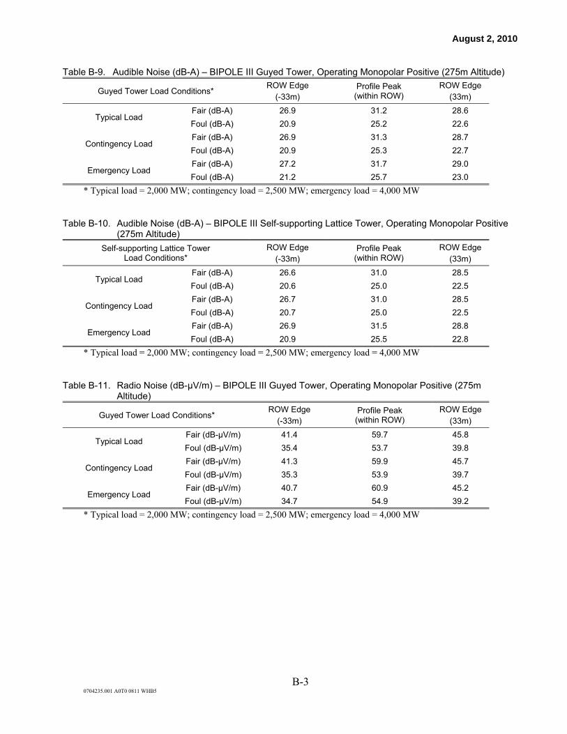
August 2, 2010
B-3 0704235.001 A0T0 0811 WHB5
Table B-9. Audible Noise (dB-A) – BIPOLE III Guyed Tower, Operating Monopolar Positive (275m Altitude)
Guyed Tower Load Conditions* ROW Edge
(-33m) Profile Peak
(within ROW) ROW Edge
(33m)
Typical Load Fair (dB-A) 26.9 31.2 28.6
Foul (dB-A) 20.9 25.2 22.6
Contingency Load Fair (dB-A) 26.9 31.3 28.7
Foul (dB-A) 20.9 25.3 22.7
Emergency Load Fair (dB-A) 27.2 31.7 29.0
Foul (dB-A) 21.2 25.7 23.0
* Typical load = 2,000 MW; contingency load = 2,500 MW; emergency load = 4,000 MW
Table B-10. Audible Noise (dB-A) – BIPOLE III Self-supporting Lattice Tower, Operating Monopolar Positive (275m Altitude)
Self-supporting Lattice Tower Load Conditions*
ROW Edge (-33m)
Profile Peak (within ROW)
ROW Edge (33m)
Typical Load Fair (dB-A) 26.6 31.0 28.5
Foul (dB-A) 20.6 25.0 22.5
Contingency Load Fair (dB-A) 26.7 31.0 28.5
Foul (dB-A) 20.7 25.0 22.5
Emergency Load Fair (dB-A) 26.9 31.5 28.8
Foul (dB-A) 20.9 25.5 22.8
* Typical load = 2,000 MW; contingency load = 2,500 MW; emergency load = 4,000 MW
Table B-11. Radio Noise (dB-μV/m) – BIPOLE III Guyed Tower, Operating Monopolar Positive (275m Altitude)
Guyed Tower Load Conditions* ROW Edge
(-33m) Profile Peak (within ROW)
ROW Edge (33m)
Typical Load Fair (dB-μV/m) 41.4 59.7 45.8
Foul (dB-μV/m) 35.4 53.7 39.8
Contingency Load Fair (dB-μV/m) 41.3 59.9 45.7
Foul (dB-μV/m) 35.3 53.9 39.7
Emergency Load Fair (dB-μV/m) 40.7 60.9 45.2
Foul (dB-μV/m) 34.7 54.9 39.2
* Typical load = 2,000 MW; contingency load = 2,500 MW; emergency load = 4,000 MW
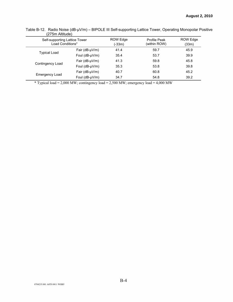
August 2, 2010
B-4 0704235.001 A0T0 0811 WHB5
Table B-12. Radio Noise (dB-μV/m) – BIPOLE III Self-supporting Lattice Tower, Operating Monopolar Positive (275m Altitude)
Self-supporting Lattice Tower Load Conditions*
ROW Edge (-33m)
Profile Peak (within ROW)
ROW Edge (33m)
Typical Load Fair (dB-μV/m) 41.4 59.7 45.9
Foul (dB-μV/m) 35.4 53.7 39.9
Contingency Load Fair (dB-μV/m) 41.3 59.8 45.8
Foul (dB-μV/m) 35.3 53.8 39.8
Emergency Load Fair (dB-μV/m) 40.7 60.8 45.2
Foul (dB-μV/m) 34.7 54.8 39.2
* Typical load = 2,000 MW; contingency load = 2,500 MW; emergency load = 4,000 MW

Appendix C Modeling results: negative pole, monopolar operation

August 2, 2011
0704235.001 A0T0 0811 WHB5
C-1
Table C-1. Electric Fields (kV/m) – BIPOLE III Guyed Tower, Operating Monopolar Negative
Guyed Tower Load Conditions* ROW Edge
(-33m) Profile Peak
(within ROW) ROW Edge
(33m)
Typical Load Fair (kV/m) -4.7 -19.1 -1.6
Foul (kV/m) -10.1 -34.1 -3.9
Contingency Load Fair (kV/m) -4.7 -19.5 -1.6
Foul (kV/m) -10.1 -34.7 -3.9
Emergency Load Fair (kV/m) -4.6 -22.1 -1.6
Foul (kV/m) -10.1 -38.8 -3.8
* Typical load = 2,000 MW; contingency load = 2,500 MW; emergency load = 4,000 MW
Table C-2. Electric Fields (kV/m) – BIPOLE III Self-supporting Lattice Tower, Operating Monopolar Negative
Self-supporting Lattice Tower Load Conditions*
ROW Edge (-33m)
Profile Peak (within ROW)
ROW Edge (33m)
Typical Load Fair (kV/m) -4.7 -19.1 -1.6
Foul (kV/m) -10.3 -34.1 -3.9
Contingency Load Fair (kV/m) -4.7 -19.5 -1.6
Foul (kV/m) -10.2 -34.7 -3.9
Emergency Load Fair (kV/m) -4.7 -22.2 -1.6
Foul (kV/m) -10.2 -38.9 -3.9
* Typical load = 2,000 MW; contingency load = 2,500 MW; emergency load = 4,000 MW
Table C-3. Magnetic Fields (mG) – BIPOLE III Guyed Tower, Operating Monopolar Negative
Guyed Tower Load Conditions* ROW Edge
(-33m) Profile Peak (within ROW)
ROW Edge (33m)
Typical Load Total (mG) 49.8 280.2 49.8
Contingency Load Total (mG) 62.5 358.9 62.5
Emergency Load Total (mG) 102.7 666.7 102.7
* Typical load = 2,000 MW; contingency load = 2,500 MW; emergency load = 4,000 MW
Table C-4. Magnetic Fields (mG) – BIPOLE III Self-supporting Lattice Tower, Operating Monopolar Negative
Self-supporting Lattice Tower Load Conditions*
ROW Edge (-33m)
Profile Peak (within ROW)
ROW Edge (33m)
Typical Load Total (mG) 51.5 284.0 51.5
Contingency Load Total (mG) 64.7 363.6 64.7
Emergency Load Total (mG) 106.4 673.7 106.4
* Typical load = 2,000 MW; contingency load = 2,500 MW; emergency load = 4,000 MW

August 2, 2011
0704235.001 A0T0 0811 WHB5
C-2
Table C-5. Ion Current Flux (nA/m2) – BIPOLE III Guyed Tower, Operating Monopolar Negative
Guyed Tower Load Conditions* ROW Edge
(-33m) Profile Peak
(within ROW) ROW Edge
(33m)
Typical Load Fair (nA/m2) -1 -34 0
Foul (nA/m2) -6 -131 -1
Contingency Load Fair (nA/m2) -1 -36 0
Foul (nA/m2) -6 -138 -1
Emergency Load Fair (nA/m2) -1 -50 0
Foul (nA/m2) -6 -187 -1
* Typical load = 2,000 MW; contingency load = 2,500 MW; emergency load = 4,000 MW
Table C-6. Ion Current Flux (nA/m2) – BIPOLE III Self-supporting Lattice Tower, Operating Monopolar Negative
Self-supporting Lattice Tower Load Conditions*
ROW Edge (-33m)
Profile Peak (within ROW)
ROW Edge (33m)
Typical Load Fair (nA/m2) -1 -34 0
Foul (nA/m2) -6 -131 -1
Contingency Load Fair (nA/m2) -1 -36 0
Foul (nA/m2) -6 -138 -1
Emergency Load Fair (nA/m2) -2 -50 0
Foul (nA/m2) -6 -188 -1
* Typical load = 2,000 MW; contingency load = 2,500 MW; emergency load = 4,000 MW
Table C-7. Ion Density (ions/cm3) – BIPOLE III Guyed Tower, Operating Monopolar Negative
Guyed Tower Load Conditions* ROW Edge
(-33m) Profile Peak
(within ROW) ROW Edge
(33m)
Typical Load Fair (ions/cm3) -12,800 -73,800 -3,700
Foul (ions/cm3) -22,250 -165,650 -5,900
Contingency Load Fair (ions/cm3) -13,000 -76,250 -3,750
Foul (ions/cm3) --23,250 -165,600 -5,900
Emergency Load Fair (ions/cm3) -13,500 -93,550 -3,900
Foul (ions/cm3) -23,400 -200,850 -6,050
*Typical load = 2,000 MW; contingency load = 2,500 MW; emergency load = 4,000 MW
Table C-8. Ion Density (ions/cm3) – BIPOLE III Self-supporting Lattice Tower, Operating Monopolar Negative
Self-supporting Lattice Tower Load Conditions*
ROW Edge (-33m)
Profile Peak (within ROW)
ROW Edge (33m)
Typical Load Fair (ions/cm3) -13,250 -73,550 -3,650
Foul (ions/cm3) -23,800 -160,600 -5,850
Contingency Load Fair (ions/cm3) -13,150 -76,000 -3,700
Foul (ions/cm3) -23,600 -165,550 -5,850
Emergency Load Fair (ions/cm3) -13,650 -93,350 -3,900
Foul (ions/cm3) -23,800 -200,850 -6,000
* Typical load = 2,000 MW; contingency load = 2,500 MW; emergency load = 4,000 MW

August 2, 2011
0704235.001 A0T0 0811 WHB5
C-3
Table C-9. Audible Noise (dB-A) – BIPOLE III Guyed Tower, Operating Monopolar Negative (275m Altitude)
Guyed Tower Load Conditions* ROW Edge
(-33m) Profile Peak
(within ROW) ROW Edge
(33m)
Typical Load Fair (dB-A) 4.5 6.4 4.5
Foul (dB-A) <1 <1 <1
Contingency Load Fair (dB-A) 4.2 6.0 4.2
Foul (dB-A) <1 <1 <1
Emergency Load Fair (dB-A) 1.9 3.8 1.9
Foul (dB-A) <1 <1 <1
* Typical load = 2,000 MW; contingency load = 2,500 MW; emergency load = 4,000 MW
Table C-10. Audible Noise (dB-A) – BIPOLE III Self-supporting Lattice Tower, Operating Monopolar Negative (275m Altitude)
Self-supporting Lattice Tower Load Conditions*
ROW Edge (-33m)
Profile Peak (within ROW)
ROW Edge (33m)
Typical Load Fair (dB-A) <1 <1 <1
Foul (dB-A) <1 <1 <1
Contingency Load Fair (dB-A) <1 <1 <1
Foul (dB-A) <1 <1 <1
Emergency Load Fair (dB-A) <1 <1 <1
Foul (dB-A) <1 <1 <1
* Typical load = 2,000 MW; contingency load = 2,500 MW; emergency load = 4,000 MW
Table C-11. Radio Noise (dB-μV/m) – BIPOLE III Guyed Tower, Operating Monopolar Negative (275m Altitude)
Guyed Tower Load Conditions* ROW Edge
(-33m) Profile Peak (within ROW)
ROW Edge (33m)
Typical Load Fair (dB-μV/m) <1 <1 <1
Foul (dB-μV/m) <1 <1 <1
Contingency Load Fair (dB-μV/m) <1 <1 <1
Foul (dB-μV/m) <1 <1 <1
Emergency Load Fair (dB-μV/m) <1 <1 <1
Foul (dB-μV/m) <1 <1 <1
* Typical load = 2,000 MW; contingency load = 2,500 MW; emergency load = 4,000 MW

August 2, 2011
0704235.001 A0T0 0811 WHB5
C-4
Table C-12. Radio Noise (dB-μV/m) – BIPOLE III Self-supporting Lattice Tower, Operating Monopolar Negative (275m Altitude)
Self-supporting Lattice Tower Load Conditions*
ROW Edge (-33m)
Profile Peak (within ROW)
ROW Edge (33m)
Typical Load Fair (dB-μV/m) <1 <1 <1
Foul (dB-μV/m) <1 <1 <1
Contingency Load Fair (dB-μV/m) <1 <1 <1
Foul (dB-μV/m) <1 <1 <1
Emergency Load Fair (dB-μV/m) <1 <1 <1
Foul (dB-μV/m) <1 <1 <1
* Typical load = 2,000 MW; contingency load = 2,500 MW; emergency load = 4,000 MW

, 2011
Appendix 2
Space charge and research on the respiratory system, mood, and behavior
November 24, 2011
2-1
0704235.001 D0T0 1111 WHB6
Space charge and research on the respiratory system, mood, and behavior
Collectively small air ions and charged aerosols are referred to as space charge. Air ions are
simply air molecules that have gained or lost electrical charges, so it is understandable that
investigations into their effects would focus on the respiratory system and the skin. The
interactions of air ions with the body are similar to interactions with other components of the air
(e.g., gases such as oxygen and nitrogen), except that charged particles can be attracted to and
deposited on the skin and respiratory tract by electrostatic forces. The deposition of particles on
the skin is the same as produced by wind (NRPB, 2004a). Consideration of such forces with
respect to the respiratory tract suggests that most of the air ions would be retained in the nose and
bronchi with few reaching the deep alveoli of the lung (MEQB, 1982). Despite many theories
offered over the years, however, no mechanism has been confirmed to explain how air ions could
exert any significant biological effect on respiratory or other systems (MEQB, 1982; NRPB,
2004a).
One mechanism by which air ions are neutralized is the transfer of charge from small air ions to
larger aerosols (charged aerosols). This route of interaction of space charge with the body has
been given less attention because ambient aerosols are already charged to some degree, and for
particles up to 1 µm, multiple charges up to 5 or 10 Q (Q = the charge on a single electron) are
quite likely (Kunkel, 1950).
Laboratory studies have demonstrated that large amounts of charge on aerosol particles increase
their deposition in the respiratory tract. Melandri et al. (1977, 1983) were able to determine the
level of charge per particle that had to be exceeded to increase deposition in the human
respiratory tract above that of uncharged particles. This particle charge threshold was as low as
Q = 9 for 0.3 µm diameter particles and as high as Q = 21-49 for 0.6 µm and 1.0 m particles.
(Common atmospheric aerosols, such as dust and pollen, are generally composed of particles 1.0
m or larger in diameter, while the particles of fumes and smoke generally have diameters less
than 1.0 µm).

November 24, 2011
2-2
0704235.001 D0T0 1111 WHB6
This work has been confirmed by Prodi and Mularoni (1985) who reported that 29 Q was
required to enhance deposition of 0.6 µm particles. Scheuch et al. (1990) reported that
conditions simulating the operation of a room ionizer in a closed room achieved about 50
charges per particle (50 Q) but increased deposition of particles in the human respiratory tract by
less than 2% (0.5 µm particles) or 6.4% (1.4 µm particles).
Hoppel (1980) has calculated an upper bound for the median charge on particles of different
sizes as a function of particle concentration and charging time for particles carried downwind of
a DC transmission line. His results suggest that few aerosol particles less than 1.0 m in
diameter would acquire a charge greater than 10 Q per particle. This is within the range of a
Maxwell-Boltzman distribution that describes the distribution of charge on aerosols under
equilibrium conditions (NRPB, 2004a), and thus does not indicate that a DC transmission line
would add sufficient charge to aerosols beyond that already present to significantly enhance
deposition.
A review of research on the DC transmission line environment by MEQB with respect to the
dosimetry of charged aerosols concluded it is unlikely that particles can be charged to a
sufficient degree or be present in high enough concentrations for this to be a problem (MEQB,
1982). Speculation as to whether exposure to ambient aerosols is increased by the addition of
electrical charge from corona on AC transmission lines has been raised on theoretical grounds,
but no supporting experimental evidence in humans has been put forth to support this specific
claim (Fews et al., 1999, 2002). Assessments of this hypothesis have criticized it on multiple
grounds (NRPB 2004a; Jeffers, 2005; WHO, 2007), including a lack of established relevance to
health (IARC, 2002). More recent modeling of aerosol charging by a DC transmission line has
confirmed that it could not add enough additional charges to aerosols to cause enhanced
deposition in the respiratory tract (Jeffers, 2007). This modeling is consistent with that of
Hoppel (1980) and with the measurements of charges on aerosols near DC transmission lines.
The above conclusions are supported by the measurements of charged aerosols around the
existing Bipole I and II DC transmission lines that suggested no increase in the fraction of
aerosols charged or the number of charges per particle (Bailey et al., (2011).

November 24, 2011
2-3
0704235.001 D0T0 1111 WHB6
Since the discovery of electrical charges on molecules in the air (Elster and Geitel, 1899), there
has been speculation about their influence on biological processes. A considerable amount of
popular and scientific literature has evolved since then; animals, humans, and lower organisms
(microorganisms, plants) have been studied to look for potential effects of space charge in the
form of small air ions and larger charged aerosols. Laboratory studies of humans and animals
have evaluated a wide range of exposures from ambient levels (about 1,000 ions/cm3), to levels
in the range of those found directly under a DC transmission line (i.e., about 100,000 ions/cm3),
and to very much higher levels (2,000,000 ions/cm3).
The effects of artificially generated air ions on humans have been studied for both experimental
and therapeutic purposes. In addition, attempts have been made to investigate naturally
occurring variations in air ion levels in relation to a variety of physiological conditions. The
reported biological and behavioral responses to air ion exposures in these studies, however, are
often inconsistent. Positive and negative air ion exposures sometimes have been reported to
exert opposite effects, while many other studies reported no effects.
The large quantity of studies that have been conducted to evaluate potential biological and
therapeutic effects of space charge provide a basis to evaluate the relevance of expected space
charge from the proposed Bipole III transmission line to human and animal health. Most of this
research has been thoroughly evaluated by the panel of scientists assembled by the MEQB
(MEQB, 1982). Their overall conclusion regarding air ions was:
In summary, while air ions appear to affect some biological processes in animals, plants, and microorganisms, there is insufficient reason to believe that acute exposures to air ions are harmful or injurious. As far as is known, all effects that have been described in animals and humans are quite mild and fully reversible, usually within a few hours. However, there are insufficient data to determine what effects, if any, might be observed with exposures to high ion concentrations over extended periods of time (MEQB, 1982, pp. 8-9).
Similar conclusions are reached in later reviews (MEQB, 1986; Bailey, 1987; Charry, 1987).
Human studies are most relevant to the assessment of potential effects in humans, and they are
inherently less susceptible to artifacts than some types of animal studies (because of behavioral

November 24, 2011
2-4
0704235.001 D0T0 1111 WHB6
and biological responses to sensory stimulation of body hair by space charge and the electric
field when present at high concentrations).1
This assessment focuses on two areas of research on human subjects with relevance to the DC
transmission line environment: 1) potential effects of space charge on the respiratory system
because it appears to be the only route of exposure for air ions with any potential health
relevance; and 2) research on the effects of air ions on mood. These areas of research are
summarized below, following a discussion of a single study of the Pacific Intertie DC
transmission line that evaluated multiple outcomes.
Study of the Pacific Intertie DC transmission line
A study sponsored by the Vermont Department of Public Service was designed to assess the
potential effects of air ions and charged aerosols on people’s respiratory and mood indicators.
The health experience of a population living near a DC transmission line was compared with a
similar population living away from the line. This cross-sectional study focused on a densely
populated community through which the Pacific Intertie DC transmission line passes (Nolfi and
Haupt, 1982). The Pacific Intertie was first energized in 1970 and runs from Washington State
to the Los Angeles area. It had been operating at ±400 kV for almost 12 years at the time the
study was conducted (1981), and was upgraded to ±500 kV in 1984. The health endpoints
surveyed among the residents included headaches, number of illness days, depression,
drowsiness, and respiratory congestion.
Participants in the study were divided into groups depending on how close they lived to the DC
transmission line corridor. The “near” group lived within 0.14 miles (225 m) of the corridor and
was subdivided into those people who lived on the edge of the corridor and those who lived
beyond it. The “far” group lived between 0.65 and 0.85 miles from the line (1 to 1.4 km).
Interviews were conducted by home visits, and all members in the household over the age of two
were included. Data were collected on 438 individuals from 128 households. The responses
from all the groups were compared, and no differences for any of the endpoint measures were
1 By and large the weight of evidence from animal studies does not indicate any adverse effects of exposure to air
ions and associated charged aerosols (MEQB, 1982, 1986).

November 24, 2011
2-5
0704235.001 D0T0 1111 WHB6
observed, indicating no acute health impacts. Study quality could have been improved by better
exposure measurements and a higher response rate. Nevertheless, the study is consistent with the
results of experimental and clinical studies reviewed below and by the MEQB (1982).
Human experimental studies of space charge
The following section evaluates experimental studies of humans exposed to air ions and charged
aerosols. These studies evaluated the effect of exposure on the respiratory system, behavior, and
mood.
Respiratory system
A systematic literature review was conducted to identify studies relevant to the effects of air ions
and space charge on respiratory effects. The MEQB prepared a detailed review of studies
relevant to this topic in 1982 (MEQB, 1982). The systematic literature review identified 22
studies including those previously reviewed by the MEQB (1982) and those published thereafter
(Table 1).2 The table describes the measured ion concentration, exposure duration, study
measures affected or not affected, and comments regarding strengths and weaknesses of each
study.
Air ion exposure levels from 1,600 ions/cm3 to 1,500,000 ions/cm3 were measured in 19 of these
studies. A wide range of respiratory measures were studied, including respiratory rate, multiple
measures of pulmonary function, and respiratory symptoms. Of note, most of the studies were
performed to test for a therapeutic effect of air ions. Many of the subjects were adults and
children with pre-existing asthma and related respiratory conditions. These studies provide no
persuasive evidence for an effect of air ions (and concomitant charged aerosols) on respiratory
effects. There was no consistency as to the direction of the response (i.e., beneficial or adverse)
or the polarity of ions to which the subjects were exposed (i.e., + or -). Furthermore, there was
no clear dose-response relationship. These conclusions are consistent with the MEQB review, 2 Yaglou et al., 1933; Herrington, 1935; Kornblueh and Griffin, 1955; Kornblueh et al., 1958; Winsor and Beckett,
1958; Zylberberg and Loveless, 1960; Yaglou, 1961; Lefcoe, 1963; Blumstein et al., 1964, Motley and Yanda, 1966; Palti et al., 1966, McDonald et al., 1967; Jones et al., 1976; Albrechtsen et al., 1978; Ben-Dov et al., 1983; Dantzler et al., 1983; Nogrady and Furglass, 1983; Wagner et al., 1983; Kirkham et al., 1984; Lipin et al., 1984; Finnegan et al., 1987; Reilly and Stevenson, 1993.

November 24, 2011
2-6
0704235.001 D0T0 1111 WHB6
which stated that only minor symptoms, e.g., throat dryness, were related to experimental ion
exposures, with limited evidence of any dose-response relationships. The MEQB also concluded
that short- and long-term exposures to positive and negative ions do not affect persons with pre-
existing allergies, asthma, or respiratory disease, or persons more sensitive to respiratory
irritants. This assessment is also consistent with a recent review by Blackhall et al. (2010) which
concluded that research has failed to demonstrate any benefit of air ionizers in the treatment of
chronic asthma in children and adults.
These studies had several limitations. Many of the studies did not report blinding the subjects or
investigators to exposure to prevent expectation or placebo effects. Some studies did not
quantitatively evaluate the respiratory response or measure the level of exposure. Furthermore,
none of the studies controlled for the reduction in particulate levels by air ionizers. Therefore,
where beneficial effects of air ionizers were reported, it is possible that the benefits resulted from
the reduction of particulate levels in the rooms (dust, allergens).
In conclusion, the research does not provide reliable evidence to support the inference that short-
term or extended exposure to air ions or charged aerosols (including levels greater than will be
produced by the proposed Bipole III project) would produce either adverse or beneficial effects
on respiratory function. This is consistent with the conclusion that charges on aerosols are of
greater significance for aerosol therapy, in which there may be hundreds to thousands of
charges/particle, than for inhalation toxicology (Isaacs et al., 2005).
Behavior and mood
Some of the earliest research on human responses to air ions focused on therapeutic behavioral
responses (e.g., Dessauer, 1931; Herrington, 1935; Silverman and Kornblueh, 1957; McGurk,
1959). Changes in air ion concentrations vary with the weather; therefore, some of the impetus
for this research was to explain people’s subjective responses to weather changes. In addition,
the speculation that exposure to negative air ions improves performance and mood was promoted
by manufacturers of air ion generators following a widely publicized article in Reader's Digest in
the 1960s. Some investigators had already formed the impression that exposure to air ions,

November 24, 2011
2-7
0704235.001 D0T0 1111 WHB6
particularly negative ions, had effects on mood and feelings of well being (Dessauer, 1931;
McGurk, 1959), stimulating research that continues to this day.
A systematic literature search was conducted to identify studies relevant to the effects of air
ions/charged aerosols on mood and well-being. Thirty English-language studies were identified
(Table 2).3 Table 2 describes the measured ion concentration, exposure duration, study measures
affected or not affected, and comments regarding strengths and weaknesses of each study.
All but two (Sigel, 1979, Yaglou, 1961) of the studies were published in peer-reviewed journals.
Air ion exposure levels were measured and reported in 23 of these studies and ranged from 1,000
ions/cm3 to 2,750,000 ions/cm3. Most studies investigated the potential effects of negative air
ions. Seven studies reported no significant response to ion treatment while the remainder
reported some type of response. These studies were grouped into four categories which are
reviewed separately below.
Observations of Relaxation and Sleepiness
Four studies evaluated relaxation and sleepiness; all reported that positive or negative air ion
exposure produced relaxation or sleepiness after exposures lasting between 0.5 and 1.5 hours.4
These studies had numerous limitations: ion levels were only measured in two studies; the
observations were not quantified or systematically evaluated in three studies; the fourth study
included only four subjects; and only one study blinded study participants to exposure.
3 Silverman and Kornbleuh, 1957; McGurk, 1959; Yaglou, 1961; Assael et al., 1974; Sigel, 1979; Charry and
Hawkinshire, 1981; Tom et al., 1981; Buckalew and Rizzuto, 1962; Baron et al., 1985; Dantzler et al., 1983; Deleanu and Stamatiu, 1985; Finnegan et al., 1987; Giannini et al., 1986/1987; Giannini et al., 1986; Hawkins, 1981; Hedge and Collis, 1987; Lips, 1987; Misiaszek et al., 1987; Reilly and Stevenson, 1993; Terman and Terman, 1995; Watanabe et al., 1997; Terman et al., 1998; Nakane et al., 2002; Iwama et al., 2004; Goel et al., 2005; Goel and Etwaroo, 2006; Terman and Terman, 2006; Giannini et al., 2007; Malcolm et al., 2009; Flory et al., 2010.
4 Silverman and Kornbleuh, 1957; Yaglou, 1961; Assael et al., 1974; Misiaszek et al., 1987.

November 24, 2011
2-8
0704235.001 D0T0 1111 WHB6
Personal comfort ratings
Six studies described personal comfort ratings after exposure to positive or negative air ions,
ranging from 10 minutes to 6-8 weeks.5 In three studies, air ions of either polarity had no effect
on personal comfort ratings with exposures of 18,000 ions/cm3, 20,000 ions/cm3, and 172,000
ions/cm3. In the remaining three studies, negative ions were reported to increase ratings of
improved personal comfort with exposures of 3,500 ions/cm3, 8,000 ions/cm3, and 50,000
ions/cm3. The rating changes in these studies were similar to or less than the small changes
associated with environmental exposures (e.g., temperature and humidity). Some precautions
were taken to minimize the subjects’ awareness of exposure conditions in all six studies.
Ratings of activation, anxiety, and mood
Twelve studies rated the subjects’ mood responses to positive or negative air ions at exposure
levels between 2,300 ions/cm3 and 100,000 ions/cm3 and durations ranging from 15 minutes to 3
days6; only one study did not measure air ion levels. Three of the studies reported no response to
ion exposures; the remainder reported a variety of responses, which were not consistent in the
direction of response to air ions compared to controls or the polarity of ions associated with the
response. Where responses were quantified, they were of very small magnitude and weaker than
those reported for other environmental factors (e.g., temperature and humidity). Negative ions
were more often reported to decrease indicators of tension, anxiety, and a lowered mood rating,
but the direction of the response often depended upon characteristics of the subjects and testing
conditions.7 Furthermore, no dose-response relationships were evident. Overall, these studies
provide no consistent evidence for the hypothesis that air ions are important modulator of subject
responses to environmental conditions.
5 McGurk, 1959; Hawkins, 1981; Finnegan et al., 1987; Lips, 1987; Reilly and Stevenson, 1993; Watanabe et al.,
1997. 6 Sigel, 1979; Charry and Hawkinshire, 1981; Tom et al., 1981; Buckalew and Rizzuto, 1962; Dantzler et al.,
1983; Baron et al., 1985; Giannini et al., 1986/1987; Giannini et al., 1986; Hedge and Collis, 1987; Nakane et al., 2002; Iwama et al., 2004; Malcolm et al., 2009.
7 For example, one of the best controlled studies reported that exposure to positive air ions increased ratings of anxiety, inattention, tension, and decreased task involvement on the first day of testing, but the subjects’ ratings were the opposite on the second day of testing, i.e., subjects exposed to (+) air ions had lower ratings of anxiety, tension, and higher task involvement (Charry and Hawkinshire, 1981).

November 24, 2011
2-9
0704235.001 D0T0 1111 WHB6
Indicators of clinical depression
Eight studies exposed patients with depression to air ions at levels between 3,000 ions/cm3 and
2,700,000 ions/cm3 for durations ranging from 1 hour on a single day to 1 hour exposures every
day for 30 days.8 Air ion levels were not measured in five of these studies. Treatment effects
were assessed by either standardized assessment ratings by clinicians or patient questionnaires.
Seven of these eight studies reported a beneficial effect associated with air ion exposure, the
exception being the study by Flory et al. (2010), who reported no response. Some studies
provided evidence of a dose-response relationship; five studies reported no clear effect of low air
ion levels (~10,000 ions/cm3), but much higher levels (2,700,000 ions/cm3) were interpreted as
producing a reduction in symptoms of depression. There was also some suggestion that daily
exposures for more than 10 to 14 days were required to produce a greater therapeutic response
(Terman and Terman, 1995, 2006; Terman et al., 1998; Goel et al., 2005).
While there appears to be some consistency in the positive responses of depressed patients to
high levels of air ions, researchers express concern that the effect is an artifact of the placebo or
expectation effect. Subject responses to treatments (and the beliefs of the investigators
themselves) often can result entirely from the subjects’ or investigators’ false beliefs that the
treatment produces a change. For beneficial effects, this is referred to as a placebo response;
conversely, the nocebo response arises from beliefs that an exposure produces harm when it is
inert. This problem is compounded when subjects are able to discern whether they have been
given a hypothesized effective or ineffective treatment and respond to questions accordingly.
For studies of mood and depression where the measure of effect is often subjective, the
magnitude of the placebo effect can be considerable.9 One investigator suggested that the
“largest component of antidepressant treatments, including bright light or negative ions, can be
the placebo effect” (Flory et al., 2010).
8 Deleanu and Stamatiu, 1985; Terman and Terman, 1995; Terman et al., 1998; Goel et al., 2005; Goel and
Etwaroo, 2006; Terman and Terman, 2006; Giannini et al., 2007; Flory et al., 2010.
9 For example, Burgess et al. (2004) report that exposure to dummy ion generators (inert boxes) each morning for
four weeks produced the same reduction in depression ratings as exposure to light in the morning or at night (hypothesized antidepressant treatments).

November 24, 2011
2-10
0704235.001 D0T0 1111 WHB6
A number of the studies have failed to report that study participants were blinded to their
exposure condition (i.e., single blinding), and an even larger number failed to report that the
study investigators were also blinded to exposure assignments (i.e., double blinding). In better
studies, such precautions are taken to minimize the potential bias on the part of the subjects and
investigators that would affect the study results. This potential bias from the subjects’
knowledge and expectations was estimated in some studies by comparing subjects’ expectations
about treatments with ratings of depression at the conclusion of the study. Some studies reported
no association between expectations and outcome, suggesting minimal bias (Terman et al., 1998;
Goel and Etwaroo, 2006), while others reported a significant association (Terman and Terman,
2006; Flory et al., 2010), suggesting a greater potential for bias.
Overall, the studies of behavior and mood in subjects exposed to air ions do not show any
consistent results with respect to relaxation and sleepiness, personal comfort ratings, and ratings
of activation, anxiety, and mood. If there is any influence of air ions on these measures, the
effect is less than is observed for small changes in other environmental factors, e.g., humidity
and temperature. While a beneficial effect on depression was observed in studies with exposures
to high levels of air ions, this is likely due to the placebo effect. Most studies had limitations in
their design and procedures. Some limitations may have led to artifactual findings, while other
limitations (e.g., small number of subjects and failure to measure ion concentrations) are
inadequacies that reduce the investigators’ ability to detect an effect, if it exists.
In conclusion, the research to date does not show that air ions at the levels and durations of
exposures that might be encountered by persons around the proposed Bipole III transmission line
have any adverse effects on behavior and mood.

November 24, 2011
2-11
0704235.001 D0T0 1111 WHB6
References
Albrechtsen O, Clausen V, Christensen FG, Jensen JG, Moller T. The influence of small atmospheric ions on human well-being and mental performance. Int J Biometeor 22:249-262, 1978.
Assael M, Pfeifer Y, Sulman FG. Influence of artificial air ionisation on the human electroencephalogram. Int J Biometeor 18:306-312, 1974.
Bailey WH. Biological responses to air ions: Is there a role for serotonin? In Charry JM, Kavet R (eds.). CRC Press, Inc.: Boca Raton Florida, 1987.
Baron RA, Russell GW, Arms RL. Negative ions and behavior: impact on mood, memory, and aggression among Type A and Type B persons. Journal of Personality and Social Psychology 48:746-754, 1985.
Ben-Dov I, Amirav I, Shochina M, Amitai I, Bar-Yishay E, Godfrey S. Effect of negative ionization of inspired air on the response of asthmatic children to exercise and inhaled histamine. Thorax 38:584-588, 1983.
Blackhall K, Appleton S, Cates CJ. Ionisers for chronic asthma. Cochrane Database of Systematic Reviews (Art. No.: CD003986. DOI: 10.1002/14651858), 2003.
Blumstein GE, Spiegelman J, Kimbel P. Atmospheric ionization in allergic respiratory diseases: a double blind study. Arch Environ Health 8:818-819, 1964.
Buckalew LW and Rizzuto A. Subject response to negative air ion exposure. Aviation, Space and Environmental Medicine 822-823, 1982.
Charry JM. Biological effects of air ions: A comprehensive review of laboratory and clinical data. In Charry JM, Kavet R (eds.). CRC Press, Inc.: Boca Raton Florida, 1987.
Charry JM and Hawkinshire FBW. Effects of atmospheric electricity of some substrates on disordered social behavior. Journal of Personality and Social Psychology 41:185-197, 1981.
Dantzler BS, Martin BG, Nelson HS. The effect of positive and negative air ions on bronchial asthma. Annals of Allergy 51:362-366, 1983.
Deleanu M and Stamatiu C. Influence of aeroionotherapy on some psychiatric symptoms. Int J Biometeor 29:91-96, 1985.
Dessauer F. Zehn Jahre Forschung auf dem Physitzalisch – Medizinischen Grenzgelbeit. Leipzig: Georg Thieme, 1931.
Elster J and Geitel H. Uber die existenz electoscher ionen in der atmosphere. Terr Mage 4:213, 1899.

November 24, 2011
2-12
0704235.001 D0T0 1111 WHB6
Fews AP, Henshaw DL, Wilding RJ, Keitch PA. Corona ions from power lines and increased exposure to pollutant aerosols. Int J Radiat Biol 75:1523-1531, 1999.
Fews AP, Wilding RJ, Keitch PA, Holden NK, Henshaw DL. Modification of atmospheric DC fields by space charge from high-voltage power lines. Atmospheric Research 63:271-289, 2002.
Finnegan NJ, Pickering CAC, Gill FS, Ashton I, Froese D. Effect of negative ion generators in sick buildings. Br Med J 294:1195-1196, 1987.
Flory R, Ametepe J, Bowers B. A randomized, placebo-controlled trial of bright light and high-density negative air ions for treatment of Seasonal Affective Disorder. Psychiatry Res 15:101-108, 2010.
Giannini AJ, Jones BT, Loiselle RH. Reversibility of serotonin irritation syndrome with atmospheric anions. J Clin Psychiatry 47:141-143, 1986.
Giannini AJ, Jones BT, Loiselle RH, Price WA. Anxiogenic effects of generated ambient cations-a preliminary study. Intl J Psychiatry in Medicine 16:243-248, 1986-87.
Giannini AJ, Giannini JD, Melemis S, Giannini JN. Treatment of acute mania with ambient air anionization: variants of climactic heat stress and serotonin syndrome. Psychological Reports 100:157-163, 2007.
Goel N, Terman M, Terman JS Macchi MM, Stewart JW. Controlled trial of bright light and negative air ions for chronic depression. Psychol Med 35:945-955, 2005.
Goel N and Etwaroo GR. Bright light, negative air ions and auditory stimuli produce rapid mood changes in a student population: a placebo-controlled study. Psychol Med 36:1253-1263, 2006.
Hawkins LH. The influence of air ions, temperature and humidity on subjective wellbeing and comfort. Journal of Environmental Psychology 1:279-292, 1981.
Hedge A and Collis MD. Do negative air ions affect human mood and performance? Ann Occup Hyg 31:285-290, 1987.
Herrington LP. The influence of ionized air upon normal subjects. J Clin Invest 14:70-80, 1935.
Herrington LP and Kuh C. The reaction of hypertensive patients in atmospheres containing high concentrations of heavy ions. J Ind Hys Toxicol 20:179-187, 1938.
Hoppel WA. Study of Drifting, Charged Aerosols from HVDC Lines. Final Report. Palo Alto: Electric Power Research Institute Report No. EL-1327, 1980.
International Agency for Research on Cancer (IARC). IARC Monographs on the Evaluation of Carcinogenic Risks to Humans: Volume 80 Non-Ionizing Radiation, Part 1: Static and Extremely Low-Frequency (ELF) Electric and Magnetic Fields. Lyon, France: World Health Organization, 2002.

November 24, 2011
2-13
0704235.001 D0T0 1111 WHB6
Isaacs KK, Rosati JA, Martenen TB. Mechanisms of Particle Deposition in Ruzer LS and NH Harley (eds). Aerosols Handbook: Measurement, Dosimetry and Health Effects. Boca Raton: CRC Press, 2005.
Iwama H, Ohmiza H, Obara S. The relaxing effects of negative air ions on ambulatory surgery patients. Can J Anaesth 51:187-188, 2004.
Jeffers D. Relative magnitudes of the effects of electrostatic image and thermophoretic forces on particles in the respiratory tract. Rad Prot Dosimetry 113:189-194, 2005.
Jeffers D. Modelling and analyses do not support the hypothesis that charging by power-line corona increases lung deposition of airborne particles. Radiat Prot Dosimetry 123:257-261, 2007
Jones DP, O’Connor SA, Collins JV, Watson BW. Effect of long-term ionized air treatment on patients with bronchial asthma. Thorax 31:428-432, 1976.
Kirkham AJT, Hawkins L, Guyatt AR, Lumley K, Horsfield K, Cumming G. The effect of air ionization on lung function in chronic asthmatics. Clinical Science - Medical Research Society Communications 67:62P-63P, 1984.
Kornbleuh IH, Piersol GM, Speicher FP. Relief from pollinosis in negatively ionized rooms. Am J Phys Med 37:18-27, 1958.
Lefcoe N. Ventilatory function after exposure to ionized air. Arch Environ Health 7:664-667, 1963.
Lipin I, Gur I, Amitai Y, Amirav I, Godfrey S. Effect of positive ionization of inspired air on the response of asthmatic children to exercise. Thorax 39:594-596, 1984.
Lips R, Salawu HT, Kember P, Probert SD. Intermittent exposures to enhances air-ion concentrations for improved comfort and increase productivity? Applied Energy 28:83-94, 1987.
Malcolm CP, Cowen PJ, Harmer CJ. High-density negative ion treatment increases positive affective memory. Psychol Med 39:1930-932, 2009.
McDonald RD, Bachman CH, Lorenz PJ. Some psyehomotor and physiological tests on humans exposed to air ions. Aerospace Med 38:145-148, 1967.
McGurk FCJ. Psychological effects of artificially produced air ions. American Journal of Physical Medicine 38:136-137, 1959.
Melandri C, Prodi V, Tarroni G, Formingnani M, DeZaiacom T, Bompane GF, Maestri G. On the deposition of unipolarly charged particles in the human respiratory tract. In: Inhaled Particles IV, Part I. Walton WH and McGovern B (eds.). Oxford:Pergamon Press, 1977.
Melandri C, Torroni G, Prodi V, DelZalacomo T, Formignani M, Lombardi CC. Deposition of charged particles in human airways. J. Aerosol Sci. 14, 657-670, 1983.

November 24, 2011
2-14
0704235.001 D0T0 1111 WHB6
Minnesota Environmental Quality Board (MEQB). Science Advisors. A health and safety evaluation of the ±400-kV DC powerline. St. Paul: Minnesota Environmental Quality Board, 1982.
Misiaszek J, Gray F, Yates A. The calming effects of negative air ions on manic patients: a pilot study. Biol Psychiatry 22:107-110, 1987.
Motley HL and Yanda R. Environmental air pollution, emphysema and ionized air. Dis Chest 50:343-352, 1966.
Nakane H, Asami O, Yamada Y, Ohira H. Effect of negative air ions on computer operation, anxiety and salivary chromogrania A-like immunoreactivity. Int J Psychophysiol 46:85-89, 2002.
National Radiological Protection Board (NRPB). Particle deposition in the vicinity of power lines and possible effects on health. National Radiological Protection Board (NRPB). Volume 15, No 1, 2004a.
Nolfi JR and Haupt RC. Effects of high voltage power lines on health: Results from a systematic survey of a population sample along the ±400-kV DC Pacific Intertie. Report for State of Vermont, Public Service Department. Montpelier, VT: Associates in Rural Development, Inc., 1982.
Nogrady SG and Furnass SB. Ionisers in the management of bronchial asthma. Thorax 38:919-922, 1983.
Palti Y, De Nour E, Abrahamov A. The effects of atmospheric ions on the respiratory system of infants. Pediatrics 38:405-411, 1966.
Pavlik I. The fate of light air ions in the respiratory pathways. Int J Biometeor 11:175-185, 1967.
Prodi V and Mularoni A. Electrostatic lung deposition experiments with humans and animals. Ann Occup Hyg 29:229–240, 1985.
Reilly T and Stevenson IC. An investigation of the effects of negative air ions on responses to submaximal exercise at different times of day. J Human Ergol 33:1-9, 1993.
Scheuch G, Gebhart J, Roth C. Uptake of electrical charge in the human respiratory tract during exposure to air loaded with negative ions. J Aerosol Sci 21 (Suppl. 1):S439-8442, 1990.
Sigel S. Bio-psychological influences of air ions in men: effects on 5-hydroxytryptamine (5HT) and mood. Unpublished Ph.D. Thesis. University of California, San Francisco. Diss Abstr E10 F918266, 1979.

November 24, 2011
2-15
0704235.001 D0T0 1111 WHB6
Silverman D and Kornbleuh IH. Effect of artificial ionization of the air on the electroencephalogram—Preliminary report. American Journal of Physical Medicine 36:352-358, 1957.
Simon NJ. Biological Effects of Static Magnetic Fields. Boulder, CO: International Cryogenic Materials Commission, Inc., 1992.
Terman M and Terman JS. Treatment of seasonal affective disorder with a high-output negative ionizer. J Altern Complement Med 1:87-92, 1995.
Terman M, Terman JS, Ross DC. A controlled trial of timed bright light and negative air ionization for treatment of winter depression. Arch Gen Psychiatry 55:875-882, 1998.
Terman M and Terman JS. Controlled trial of naturalistic dawn simulation and negative air ionization for seasonal affective disorder. Am J Psychiatry 163:2126-2133, 2006.
Tom G, Poole MF, Gaila J, and Berrier J. The influence of negative air on human performance and mood. Human Factors 23:633-636, 1981.
Wagner CJ, Danziger RE, Nelson HS. Relation between positive small air ions, weather fronts and pulmonary function in patients with bronchial asthma. Annals of Allergy 51:430-435, 1983.
Watanabe I, Noro H, Ohtsuka Y, Mano Y, Agishi Y. Physical effects of negative air ions in a wet sauna. Int J Biometeorol 40:107-112, 1997.
Winsor T and Beckett JC. Biologic effects of ionized air in man. Am J Phys Med 37, 83-89, 1958.
World Health Organization (WHO). Environmental Health Criteria 238: Extremely Low Frequency (ELF) Fields. Geneva, Switzerland: World Health Organization, 2007.
Yaglou CP, Brandt AD, Benjamin LC. Observation of a group of subjects before, during, and after exposure to ionized air. J Ind Hygiene 15:241-353, 1933.
Yaglou CP. Are Air Ions a Neglected Biological Factor? In: The Air We Breathe, Farber SM (ed.). Springfield, Illinois: Charles C. Thomas Publisher, 1961.
Zylberberg B and Loveless MH. Preliminary experiments with ionized air in asthma. J Asthma 31:370-374, 1960.

November 24, 2011
2-16
0704235.001 D0T0 1111 WHB6
Table 2-1. Studies of air ions and respiratory parameters
Study Author(s), Year
Ion Polarity
Ion Concentration (ions/cm3) Exposure
Duration Parameters NOT Affected
by Ion Exposure Effects Reported Design QA
Yaglou et al., 1933
(-) 5.0 x 10² - 1.5 x 10⁶ 1 hr (30
min - 3 hrs) Respiration rate
Strengths: Ss blinded Weaknesses: No blinded analysis; test subject randomization not reported. (+) 1.0 x 10⁴ - 1.25 x 10⁶
Herrington, 1935 (-) / (+) 5.0-6.0 x 10⁶ 30 min Respiratory rate
Strengths: Detailed description of procedure Weaknesses: Ss not blinded; no blinded analysis; test subject randomization not reported.
Kornblueh and Griffin, 1955
(-) < 1.0 x 10⁴ 10-110 min 17/27 patients reported partial or complete reduction in symptoms of allergy and asthma.
Weaknesses: Exact ion concentrations not measured or reported; no quantitative measures reported; subjective relief in symptoms assessed; blinded analysis and test subject randomization not reported.
Kornbleuh et al., 1958
(-) 1.2-2.6 x 10³ 12-50 min 37/37 patients without symptoms at time of exposure not affected
34/54 symptomatic patients reported relief of hay fever and asthma symptoms.
Weaknesses: No quantitative measures reported; subjective relief in symptoms assessed; Ss not blinded; blinded analysis and test subject randomization not reported. (+) 2.0-6.5 x 10³ 12-50 min
4/5 symptomatic patients reported no relief of hay fever and asthma symptoms; 6/10 asymptomatic patients experienced symptoms with exposure.
Winsor and Beckett, 1958
(-)
3.2 x 10⁴
20 min 9/13 subjects: no symptoms
4/13 subjects: slight dryness, irritation of nose and throat. Strengths: Ss blinded, S beds
grounded Weaknesses: Few quantitative measures reported; subjective reports of symptoms assessed; other experiments assessing duration of symptoms and effects of switching from (+) to (-) ions also conducted; blinded analysis and test subject randomization not reported.
(+)
20 min Increase in symptoms in all subjects (headache, nasal obstruction, sore throat, etc). "All symptoms were mild."
2 x 15 min Increase in symptoms in 17/20 subjects
10 min Increased upper airway congestion

November 24, 2011
2-17
0704235.001 D0T0 1111 WHB6
Study Author(s), Year
Ion Polarity
Ion Concentration (ions/cm3) Exposure
Duration Parameters NOT Affected
by Ion Exposure Effects Reported Design QA
Zylberberg and Loveless, 1960
(-) NR 120 min Symptoms of wheezing or dyspnea
Strengths: Double blind, randomized study Weaknesses: Subjects exposed to (-) and (+) ions in random order; no control group evaluated.
(+) NR 120 min
Yaglou, 1961
(-) 5.0-10.0 x 10³ 1-2 hrs
Respiration rate; no effect on subjective rating of air quality or symptoms.
Strengths: Ss blinded, grounded bed Weaknesses: Test subject randomization not reported.
(+) 5.0-10.0 x 10³ 1-2 hrs
Some subjects reported irritation of respiratory tract. Authors point out that the "experiments were made during the winter, when upper respiratory symptoms were common."
(-) 2.0-4.0 x 10³ 2 x 2
hrs/day for 14 days
No effect on respiration rate of malnourished infants.
Lefcoe, 1963
(-) 1.25 x 10⁵ 4 hrs Pulmonary function tests (forced vital capacity, forced expiratory volume, and maximum mid-expiratory flow rate), symptoms of bronchial asthma.
Strengths: Ion measurements taken every hr during control, exposure and post-exposure periods; most subjects tested in 3 separate runs on separate days; values reported as percentage of control mean values. Weaknesses: Blinded analysis and test subject randomization not reported, insufficient data provided for adequate evaluation.
(+) 1.25 x 10⁵ 4 hrs
Blumstein et al., 1964
(-) 1.0 x 10⁴.
1.0 x 10⁴
30 min, 5 consecutive
days
Six measures of pulmonary function, subjective symptom relief, did not differ by exposure treatment in patients with respiratory allergy, asthma, or pulmonary emphysema.
None Strengths: Double blind, direct evaluation of placebo effect
(+)
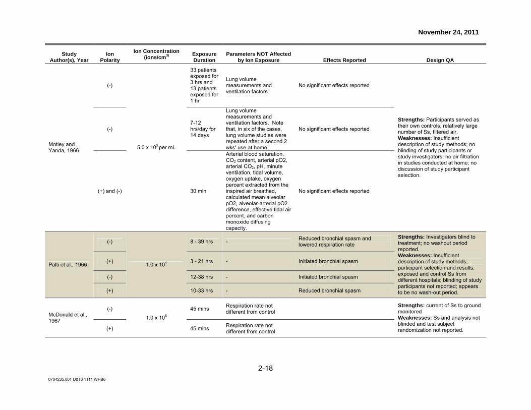
November 24, 2011
2-18
0704235.001 D0T0 1111 WHB6
Study Author(s), Year
Ion Polarity
Ion Concentration (ions/cm3) Exposure
Duration Parameters NOT Affected
by Ion Exposure Effects Reported Design QA
Motley and Yanda, 1966
(-)
5.0 x 10⁵ per mL
33 patients exposed for 3 hrs and 13 patients exposed for 1 hr
Lung volume measurements and ventilation factors
No significant effects reported
Strengths: Participants served as their own controls, relatively large number of Ss, filtered air. Weaknesses: Insufficient description of study methods; no blinding of study participants or study investigators; no air filtration in studies conducted at home; no discussion of study participant selection.
(-) 7-12 hrs/day for 14 days
Lung volume measurements and ventilation factors. Note that, in six of the cases, lung volume studies were repeated after a second 2 wks' use at home.
No significant effects reported
(+) and (-) 30 min
Arterial blood saturation, CO2 content, arterial pO2, arterial CO2, pH, minute ventilation, tidal volume, oxygen uptake, oxygen percent extracted from the inspired air breathed, calculated mean alveolar pO2, alveolar-arterial pO2 difference, effective tidal air percent, and carbon monoxide diffusing capacity.
No significant effects reported
Palti et al., 1966
(-)
1.0 x 10⁴
8 - 39 hrs - Reduced bronchial spasm and lowered respiration rate
Strengths: Investigators blind to treatment; no washout period reported. Weaknesses: Insufficient description of study methods, participant selection and results, exposed and control Ss from different hospitals; blinding of study participants not reported; appears to be no wash-out period.
(+) 3 - 21 hrs - Initiated bronchial spasm
(-) 12-38 hrs - Initiated bronchial spasm
(+) 10-33 hrs - Reduced bronchial spasm
McDonald et al., 1967
(-)
1.0 x 10⁶
45 mins Respiration rate not different from control
Strengths: current of Ss to ground monitored Weaknesses: Ss and analysis not blinded and test subject randomization not reported. (+) 45 mins
Respiration rate not different from control

November 24, 2011
2-19
0704235.001 D0T0 1111 WHB6
Study Author(s), Year
Ion Polarity
Ion Concentration (ions/cm3) Exposure
Duration Parameters NOT Affected
by Ion Exposure Effects Reported Design QA
Jones et al., 1976
(-) NR
4 wks placebo; 8 wks active; 4 wks no ionizer
No significant difference among three time periods in clinical-subjective combined score. Effects measured as morning and evening PEFR scores.
Weaknesses: Not randomized. No control group, wide age range, small numbers
Albrechtsen et al, 1978
(-) 8 x 10³ 8 min
Respiratory rate
Strengths: Measured ion mobility, grounded Ss, constant humidity, temperature; controlled, well-described experiment Weaknesses: No selection criteria
(+) 1 x 10⁴ 8 min
(-) 15 min
Respiratory rate
(+) 15 min
Ben Dov, 1983
(-) 4.0-10.0 X10⁵
2, 6 min exercise tests, 3-24 hrs apart
Breathing ionized air for 10 mins did not significantly change lung function (FEV1) of children.
Breathing ionized air significantly reduced exercise induced asthma/bronchial reactivity.
Strengths: Double blind study Weaknesses: No details of severity reported, inclusion and exclusion criteria not stated, not randomized, ozone contamination "negligible" but even trace amounts would have been inhaled because of mouthpiece.
(-) 4.0-10.0 X10⁵
histamine challenge tests 24 hrs apart
Histamine results inconclusive
Danzler et al., 1983
(-) 1.0 x 10⁵ 6 hrs FEV and somatic symptoms reported did not differ significantly from baseline or between (-) and (+) ion exposures.
Strengths: Double blind study; measured ions and grounded Ss; pulmonary measurements taken at 15, 30, 120, 240, and 360 min during exposures Weaknesses: No selection criteria and control period, data on symptoms not quantified
(+) 1.0 x 10⁵ 6 hrs

November 24, 2011
2-20
0704235.001 D0T0 1111 WHB6
Study Author(s), Year
Ion Polarity
Ion Concentration (ions/cm3) Exposure
Duration Parameters NOT Affected
by Ion Exposure Effects Reported Design QA
Nogrady and Furnglass, 1983
(-) >1.5 x 10⁵
2 x 8-wk periods with 4-wk washouts; ioniser active from 10PM-8AM daily
PEFR; symptom score; and bronchodilator consumption
Strengths: Double-blind; dust measurements taken; included a wash-out period Weaknesses: Randomization method unclear; differences in baseline PEF; non-validated symptom scale
Wagner et al., 1983
(-) 500-1,600 32 days PEFR (4 tests/day) for 48 days
Weaknesses: No selection criteria; single blind; ions measured at a single regional monitor distant from S residence; analyses incomplete; (-) ions measured but NR. (+) 500-1,600 32 days
Kirkham et al., 1984
(-) NS 4 wks, 8 hrs per night
Lung 'mechanics' measure by whole body plethysmography; gas mixing (nitrogen washout)
Strengths: Ss blinded Weaknesses: Summary results only, no test results reported; method of blinding not described; not randomized; diagnostic criteria not given; no subjective information after testing; control number not reported; no measures of ion concentration.
Lipin et al., 1984 (+) 5-10 x 105
10 min, then 6 min with exercise, repeated in 24 hrs
Exercise tests for minute ventilation, oxygen consumption, baseline FEV in asthmatic children
Post exercise fall in FEV1 significantly greater in exposed. 8/12 subjects developed more exercise-induced asthma and two subjects less, two no difference.
Strengths: Double blind; exposure delivered direct to mouth Weaknesses: No clear randomization. Inclusion and exclusion criteria not given.
Finnegan et al., 1987
(-) 1.84 x 10³ 6-8 wks
Daily ratings of personal comfort (5 measures) and environmental comfort (4 measures); upper respiratory symptoms
Proportion of Ss with upper respiratory tract infections during exposed period > control period
Strengths: Daily ion measurements; Ss blinded; ratings adjusted for temp and RH Weaknesses: No random assignment; no symptom data reported

November 24, 2011
2-21
0704235.001 D0T0 1111 WHB6
Study Author(s), Year
Ion Polarity
Ion Concentration (ions/cm3) Exposure
Duration Parameters NOT Affected
by Ion Exposure Effects Reported Design QA
Reilly and Stevenson, 1993
(-) 1.72 x 10⁵
30 min pre-test + 40 min during test
No differences in VO2 or VE at submax or maximal exercise with (-) ions; difference in VO2 and VE between rest and both exercise conditions significantly greater with (-) ions
Oxygen uptake (VO2) and ventilation (VE) significantly reduced at rest with (-) ions
Strengths: Ss blinded Weaknesses: Not known if analyses conducted in blinded manner or if test subjects were randomized; evaluations at 1:30, 10:00, 14:00 and 18:00 hrs; perceived exertion during 40 min submax and maximum exercise; significant inter-subject variability in all physiological measures.
Warner et al., 1993
NR NR
6 wks of active ioniser in home followed by 6 wks of placebo ioniser in home
PEFR, night time wheeze, daytime wheeze, nighttime cough, daytime cough, daytime activity, medication
Strengths: Double-blind; placebo-controlled Weaknesses: Randomization method unclear; residential exposure only
Abbreviations key: f = female; fev = forced expiratory volume; hr = hour; m = male; min = minute; mo = month; NS = not specified; NR = not reported; PEF = peak expiratory flow; PEFR = peak expiratory flow rate; pO2= partial pressure of oxygen; VO2 = oxygen update; VE = ventilation; wk = week; yr = year

November 24, 2011
2-22
0704235.001 D0T0 1111 WHB6
Table 2-2. Studies of air ions and mood Study
Author(s), Year
Ion Polarity
Ion Concentration
Exposure Duration
Parameters NOT Affected by Ion
Exposure Effects Reported Design QA
Silverman and Kornbleuh, 1957
(-)
NR
30 min
Transient decrease in EEG alpha frequency in most subjects; half of subjects reported dryness of mouth and upper respiratory tract, relaxation and sleepiness with ionization (slightly more frequent for (-) than (+) ion exposure)
Blinded analysis and test subject randomization not reported; small sample size
(+) 30 min
McGurk, 1959
(-) 8.0 x 10³ 5 hrs
A significant percent of subjects appeared to detect ionization condition despite blinding and reported more pleasant feelings.
Strengths: Ss blind to exposures Weaknesses: Blinded analysis and test subject randomization not reported.
(+) 8.0 x 10³ 2 hrs
Subjects reported more unpleasant feelings.
Yaglou, 1961
(-)
5.0-10.0 x 10³ 1-2 hrs No effect on subjective rating of mood or symptoms
Strengths: Ss blind to exposures Weaknesses: Blinded analysis and test subject randomization not reported.
(+)
(-) 2.0-4.0 x 10³ 2 x 2 hrs/day for 14 days
Infants appeared quieter and cried less.
Blinded analysis and test subject randomization not reported.
Assael et al., 1974
(-) 3.5 x 10⁵ 45 mins EEG changes not observed in patients given tranquilizers
Increase amplitude and synchronization of EEG with decrease in alpha frequency. Subjective reports of relaxation with ionization
Strengths: Subjects given tranquilizers first tested with placebo and double blinded. Weaknesses: All results are in the form of EEGs. The authors interpret a decrease in alpha frequency as relaxation.

November 24, 2011
2-23
0704235.001 D0T0 1111 WHB6
Study Author(s),
Year Ion
Polarity Ion
Concentration Exposure Duration
Parameters NOT Affected by Ion
Exposure Effects Reported Design QA
Sigel, 1979 (+)/(-) 1.0 x 10⁵ 2 hrs
Ion exposure (+) or (-) did not affect mood ratings relating to tension, depression, anger, fatigue, or confusion.
Mood alterations: higher vigor and friendliness in ionized subjects
Strengths: Randomly assigned to exposure conditions, data presented as mean values for each 15-min interval during exposure period Weaknesses: Blinded analyses not reported
Charry and Hawkinshire, 1981
(+) 2.0-3.0 x 10⁴
1.5 hrs positive ion exposure, 3-day wash-out period, 1.5 hrs ambient exposure
Mood alterations as indicated by decreased attention and task involvement and increased tension and anxiety. A measure of low-lability autonomic response identified by decreased skin conductance (arousal) High lability displayed increased skin conductance.
Strengths: Participants blind to treatment; controlled trial; relatively large number of participants Weaknesses: Insufficient description of study methods
Tom et al., 1981
(-) 16,160 ions/cm3 15 mins No effect on mood, sociability, or relaxed state subtests
Strengths: Controlled experiment; random assignment; double-blinded; temperature and humidity controlled; time of day controlled Weaknesses: Control n and experimental n not specified; baseline characteristics of total group only, not control and experimental Ss; S pool not described & exclusions & withdrawals not mentioned; randomization method not stated; outcome variable--one item on a questionnaire with 5 items total--no information concerning the reliability and validity of the questionnaire.

November 24, 2011
2-24
0704235.001 D0T0 1111 WHB6
Study Author(s),
Year Ion
Polarity Ion
Concentration Exposure Duration
Parameters NOT Affected by Ion
Exposure Effects Reported Design QA
Buckalew and Rizzuto, 1982
(-) NR 6 hrs Anxiety (TMAS)
Subjective feelings of relaxations. Reductions in irritability, depression and tenseness. Increases in calmness and stimulation. Improved mood or psychological states.
Strengths: Double blind. Exposed and controls matched on age, education, smoking. Weaknesses: Ion concentration not reported. Mood index was self report. No base line data either group.
Baron et al., 1985
(-) 4 x 10⁴/cm3
7.0-8.0 x 10⁴/cm3 20 min
Non-angry depression ration: no difference was noted in the pleasantness scale although only the raw scores were shown.
For the non-angry subjects: Feelings of depression, anger, and fatigue "generally" decreased as the ion concentration increased. For the angry subjects: Feelings of depression, anger, and fatigue increased as the ion concentration increased. Results interpreted as increased arousal or activation.
Randomization method: no mention of randomization. Blinding: subjects were blinded. Subject pool: male undergraduates fulfilling a course requirement. Excluded: not mentioned. Withdrawals: not mentioned. Baseline characteristics: all male undergraduates. Strengths: Controlled experiment; subjects were blinded; ion concentrations measured; Ss grounded. Weaknesses: Researchers were not blinded; unclear if Ss were randomly assigned to the ion groups; small number of Ss.
Dantzler et al., 1983
(-)
6-10 x 104 6 hrs
Three questionnaires on symptom and mood changes, including mood, energy level, sociability, tension level, and concentration.
Weaknesses: No selection criteria; double blind; measured ions and grounded Ss; no control period; questionnaire data NR; questionnaires not validated.
(+)
Deleanu and Stamatiu, 1985
(-) 1-1.5 x 10⁴/cm3
Daily, 10-30 days, 15 min or up to 50
min
Aggravation of psychiatric symptoms
Exposure ameliorated symptoms reported by patients for astenia, depression. Favorable results for sleep normalization.
Weaknesses: No control groups, no mention of blinding, results subjective, qualitative, descriptive. No tabular results. Results not explained clearly.
Finneagan et al., 1987
(-) 1.84 x 10³ 6-8 wks Daily ratings of 5 personal comfort and 4 environmental comfort ratings
Strengths: Daily ion measurements; ratings adjusted for temp and RH. Weaknesses: Ss were workers in a 'sick bldg'; no random assignment; no symptom data reported. (-) 1.84 x 10³ 6-8 wks

November 24, 2011
2-25
0704235.001 D0T0 1111 WHB6
Study Author(s),
Year Ion
Polarity Ion
Concentration Exposure Duration
Parameters NOT Affected by Ion
Exposure Effects Reported Design QA
Giannini et al., 1986/1987
(+) 2 -2.3 x 10³/cm3 2 hours BRPS, psychiatric scale. Rise in symptoms of anxiety and excitement.
Strengths: Double blind, 2 raters. Weaknesses: Subjective data only
Giannini et al.., 1986
(-) NR 20 min Anxiety and tension in prionization with anions.
Cations increase anxiety, suspicion, and excitement. Follow up exposure to anions reduced anxiety tension, suspiciousness and excitement.
Strengths: double blind. BPRS for all subjects. Weaknesses: Tables of results not consistent with method in text. Overall mean of BPRS not reported. (+) 2.x 103/cm3 20 min
Hawkins, 1981
(-) 2-3.5x 10³
Ss rated (-) ion periods as slightly warmer and fresher ENV & give slightly higher PERS ratings for warmth and alertness; higher ratings of comfort, pleased alert during night shift in area 3.
Double blind; ion measurements; data from area 2 partial reported; inadequate methods and analysis.
(+) 50-125
8 wks on; 4 wks off (areas 1 & 2); 4 wks on; 8 wks off (area 2).
Hedge and Collins, 1987
(-) 2x 10⁴ ions/cm3 placebo 2.5x10²
3 consecutive working days
Stress, arousal, cognitive task performance
No effects reported.
Validated tests used for mood, both a control and a placebo used: randomization of the 3 treatments for each individual. Double blind until ionization turned on.
Lips, 1987 (-) 5 x 10⁴ions/cm3 of
air
Ionisers continuously
turned on 9AM-5PM
Thermal comfort scores
Subjects' assessments of both their own well-being and the quality of the environment improved significantly.
Strengths: Controlled trial. Weaknesses: No randomization; outcome based on self report; small study size.

November 24, 2011
2-26
0704235.001 D0T0 1111 WHB6
Study Author(s),
Year Ion
Polarity Ion
Concentration Exposure Duration
Parameters NOT Affected by Ion
Exposure Effects Reported Design QA
Misiaszek et al., 1987
(-)
4-6 x 10⁴ sm ions
50-1000 med ions,
50-4000 lg ions
1 hr
All subjects fell to sleep, reported being calm afterwards; manic behavior reappeared 5-10 min after treatment
No control exposures; unblinded study; small sample size (4).
5-7 x 10⁴ sm ions,
70,000, 50-3200 med
ions, 50-7000 lg ions
1.5 hrs
3/4 subjects fell to sleep, 1 subject appeared less agitated; manic behavior reappeared 5-10 min after treatment
Small sample size (4).
Reilly and Stevenson, 1993
(-) 1.72 x 10⁵ 30 mins pre-
test + 40 mins during test
No effect on pre- or post-exercise anxiety, state anxiety or perception of effort.
Subjects blinded to exposure conditions; not known if analyses conducted in blinded manner or if test subjects were randomized; no description of methods or quantitative summary of results.
Terman and Terman, 1995
(-) 1.0 x 10⁴ 2.7 x 10⁶
20 min x 20 days
Lower scores on the SIGH-SAD scale indicating improvement in depression. Improvement noted on both subscales.
Strengths: Experiment; random assignment; apparently double blinded. Weaknesses: Subject pool not described; excluded & withdrawal of Ss not mentioned; significant difference in ages between groups; randomization method not stated; Ss self-exposed at home; ion concentrations not measured; in the procedure section, two outcome scales were described but in the results section only one was discussed.

November 24, 2011
2-27
0704235.001 D0T0 1111 WHB6
Study Author(s),
Year Ion
Polarity Ion
Concentration Exposure Duration
Parameters NOT Affected by Ion
Exposure Effects Reported Design QA
Terman et al., 1998
(-)
1.0 x 10⁴ ions/cm3
10,000 2.7 x 10⁶ ions/cm3
30 min x 10-14 days
Improved depression rating of 16-20% and 5-10% remission rate. This response was described as “ineffective.”
Improved depression rating of 42-50% and 20-40% remission rate. Described as a "small effect" in P1 and "large effect" in P2.
Strengths: Raters of depression status were blinded; several tests given to volunteers--must fulfill certain criteria to be included. Weaknesses: No measurements of ion concentration; randomization method not stated; S characteristics not described; unclear if the subjects receiving the negative air ionization were blinded; Ss self-exposed at home; the absence of a relation between the Ss expectation of benefit and result is contrary to experience; baseline characteristics given for the total group--not individual treatment groups.
Nakane et al., 2002
(-) 5.5-7.3 x 10³
Either 40 minutes
during task or 30 minutes post-task
(-) ions during task or during post-task recovery period reduced State-Trait Anxiety Inventory, Anxiety State (STAI-S) scores.
Strengths: Exposures randomized and subjects blinded to exposure conditions. Weaknesses: Small sample size (n = 4).
Iwama et al., 2004
(-) 1000 parts/mL
Length of surgery; exact
time not specified
Degree of tension reported by study participants during first or latter half of surgery significantly reduced among ion-exposed group.
Strengths: Controlled trial. Weaknesses: No blinding of patients reported; no randomization; outcome based on self report.

November 24, 2011
2-28
0704235.001 D0T0 1111 WHB6
Study Author(s),
Year Ion
Polarity Ion
Concentration Exposure Duration
Parameters NOT Affected by Ion
Exposure Effects Reported Design QA
Goel et al., 2005
(-)
High density=4.5 x 10¹⁴ ions/s Low-density, control group=1.7 x 10¹¹ ions/s
1 hr upon wakening for 5
wks
Melatonin onset, sleep onset, sleep midpoint, and sleep offset
Improved SIGH-SAD total score, Hamilton subscale, and atypical symptom subscale
Strengths: Controlled double-blind trial. Weaknesses: Effects compared to low, negative ion exposure, rather than no exposure; small sample size.
Goel and Etwaroo, 2006
(-)
High density=4.5 x 10¹⁴ ions/s Low-density,
control group=1.7 x 10¹¹ ions/s
30 mins for three
consecutive evenings
Likert scale ratings of perceptual characteristics and some moods (anger, vigor, tension, fatigue, and confusion).
Reduced depression scores after 15-30 min
Strengths: Controlled trial; relatively large number of participants; controlled for seasonal effects. Weaknesses: No blinding; effects compared to low, negative ion exposure, rather than no exposure.
Terman and Terman, 2006
(-) 1.7 x 10¹¹ ions/s4.5 x 1014 ions/s
93 minutes
The Atypical Symptom Scale did not show significant group effect with raw scores but did when percentage improvement was used.
For the SIGH-SAD scores the improvement in the low-density ion group was significantly lower than the high-density ion group (and other non-ion groups as well). The Hamilton-D scale also showed a significant group effect.
Strengths: Random assignment of Ss; raters blinded; extensive entry criteria Weaknesses: Randomization method not stated; Withdrawals- 126 subjects entered; 118 completed and reasons given. 99 were analyzed (additional cases were excluded after the data was analyzed); Unclear as to the validity of the removal of subjects after initial analysis has been completed--rationale was given.

November 24, 2011
2-29
0704235.001 D0T0 1111 WHB6
Study Author(s),
Year Ion
Polarity Ion
Concentration Exposure Duration
Parameters NOT Affected by Ion
Exposure Effects Reported Design QA
Giannini et al., 2007
(-) 3 x 10³/cm3 60 mins
No effect of order for treatment versus sham. No significant difference in pre-and post-treatment scores for individual items.
Significant reduction in manic symptoms on BPRS score.
Strengths: Two raters for BRS. Weaknesses: No biochemical measures. Subjects varied in days under med treatment. Began with 24 subjects but ended with 20, no explanation.
Watanabe et al., 1997
(-) 2.0 x 10⁴ ions/cm3 10 mins
No difference was noted in the pleasantness scale although only the raw scores were shown.
Strengths: Controlled experiment; S pool not described & exclusion and withdrawals of Ss not described; Ss were blinded; time of day, temperature, humidity were controlled. Weaknesses: Researchers were not blinded; subjects were both control and experimental groups; "Pleasantness scale" was just one of four items that were asked by an interviewer. No information regarding the reliability and validity of the questionnaire.
Malcolm et al., 2009
(-) NR
30 mins prior to testing + 60
mins during testing
Facial expression recognition and dot-probe tasks.
Association between Beck Depression Inventory score and treatment; increased recall and recognition of positive terms versus negative terms
Strengths: Subjects randomly assigned to exposure groups and blinded to exposure conditions. Weaknesses: Not reported if analyses conducted in blinded manner; Insufficient description of study methods.
Flory et al., 2010
(-) 4.0 x 10³ (control)
≥ 2.0 x 10⁶
(exposed)
30 mins x 12 days
Ratings of depression – two scales (HAM-D, BDI); remission rate criteria; symptoms of SAD; comparisons of ion groups to placebo group (red light) shows strong placebo effect.
Strengths: Measurements of ion and ozone concentrations; independent treatment groups; multiple measures of symptoms; inclusion & exclusion criteria; Ss randomly assigned to test groups; assessment of placebo effects. Weaknesses: Ss assembled and tested over 5 yrs; no true unexposed control group ; post-hoc inappropriate merging of groups for some analyses; no statistical analysis of % subjects; no validation of treatment expectation questionnaire.
Abbreviations key: hr = hour; m = medium; min = minute; n = number; NR = not reported; Ss= subjects; wk = week.

Health Sciences and Electrical and Semiconductors Practices
Modeling of the Electrical Environment for Proposed AC Components of the Bipole III Project

0704235.001 A0T0 0411 WHB5
Modeling of the Electrical Environment for proposed AC Components of the Bipole III Project Prepared for Manitoba Hydro Prepared by Exponent 17000 Science Drive Suite 200 Bowie, MD 20715 April 23, 2011 Exponent, Inc.

0704235.001 A0T0 0411 WHB5
Notice At the request of Manitoba Hydro, Exponent conducted specific modeling and evaluations of
components of the electrical environment of the Bipole III project. This report summarizes work
performed to date and presents the findings resulting from that work. In the analysis, we have
relied on geometry, material data, usage conditions, specifications, regulatory status, and various
other types of information provided by the client. We cannot verify the correctness of this input
data, and rely on the client for the data’s accuracy. Although Exponent has exercised usual and
customary care in the conduct of this analysis, the responsibility for the design and operation of
the project remains fully with the client.
The findings presented herein are made to a reasonable degree of engineering and scientific
certainty. Exponent reserves the right to supplement this report and to expand or modify
opinions based on review of additional material as it becomes available, through any additional
work, or review of additional work performed by others.
The scope of services performed during this investigation may not adequately address the needs
of other users of this report, and any re-use of this report or its findings, conclusions, or
recommendations presented herein are at the sole risk of the user. The opinions and comments
formulated during this assessment are based on observations and information available at the
time of the investigation. No guarantee or warranty as to future life or performance of any
reviewed condition is expressed or implied.

April 23, 2011
0704235.001 A0T0 0411 WHB5
ii
Contents
Page
List of Figures iii
List of Tables iv
Acronyms and Abbreviations v
Introduction 1
Methods 2
AC electric and magnetic field calculations 2
AC audible noise calculations 2
AC radio noise calculations 3
Modeling Results for the 230-kV Transmission Lines in the Corridor 4
Electric fields 8
Audible noise 9
Radio noise 10
Assessment Criteria and Conclusions 11
AC electric and magnetic fields 11
AC audible noise 11
AC radio noise 12
Conclusions 12
References 13 Appendix A - Input data for AC EMF, AN, and RN modeling of the
Corridor
Appendix B – Exponent’s report on EMF and health

April 23, 2011
0704235.001 A0T0 0411 WHB5
iii
List of Figures
Page
Figure 1. Location of existing 230-kV AC transmission lines and proposed Bipole III AC 230-kV transmission lines 4
Figure 2. Configuration of the corridor (view facing north). 5
Figure 3. Calculated magnetic field profile under average loading conditions with Keeyask generation and the Keewatinoow Converter Station operating. 6
Figure 4. Calculated AC electric field profile for the proposed cross-section in the Corridor 8
Figure 5. Calculated AC AN profile in foul weather conditions for the proposed cross-section in the Corridor. AN under fair weather conditions will be 25 dbA lower than the levels shown above. 9
Figure 6. Calculated AC RN profile in foul weather conditions for the proposed cross-section in the Corridor calculated at 0.5 MHz. RN levels under fair weather will be 17 dBV/m lower than those shown above. 10

April 23, 2011
0704235.001 A0T0 0411 WHB5
iv
List of Tables
Page
Table 1. AC magnetic field (mG) and AC electric field (kV/m) at specified locations 7
Table 2. Electric field (kV/m) for the transmission corridor 8
Table 3. Audible noise from the AC lines at specified locations under fair and foul weather 9
Table 4. Radio noise from the AC lines at specified locations under fair and foul weather 10

April 23, 2011
v 0704235.001 A0T0 0411 WHB5
Acronyms and Abbreviations
AC Alternating current
AM Amplitude modulated
AN Audible noise
BPA Bonneville Power Administration
Corridor The Henday-Keewatinow Transmission Corridor
dB Decibels
dB-A Decibels on the A-weighted scale
DC Direct current
EPRI Electric Power Research Institute
FM Frequency modulated
Hz Hertz
km Kilometre
ICES International Committee on Electromagnetic Safety
ICNIRP International Commission on Non-Ionizing Radiation Protection
kV Kilovolts
m Metre
mHz Megahertz
mT millitesla
MVA Megavolt ampere
MW Megawatt
NRPB National Radiological Protection Board
RN Radio noise
ROW Right-of-way
rms Root mean square
SPL Sound pressure level
µPa Micropascal
µVm microvolt/metre
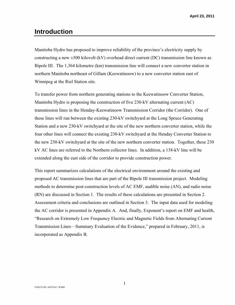
April 23, 2011
1 0704235.001 A0T0 0411 WHB5
Introduction
Manitoba Hydro has proposed to improve reliability of the province’s electricity supply by
constructing a new ±500 kilovolt (kV) overhead direct current (DC) transmission line known as
Bipole III. The 1,364 kilometre (km) transmission line will connect a new converter station in
northern Manitoba northeast of Gillam (Keewatinoow) to a new converter station east of
Winnipeg at the Riel Station site.
To transfer power from northern generating stations to the Keewatinoow Converter Station,
Manitoba Hydro is proposing the construction of five 230-kV alternating current (AC)
transmission lines in the Henday-Keewatinoow Transmission Corridor (the Corridor). One of
these lines will run between the existing 230-kV switchyard at the Long Spruce Generating
Station and a new 230-kV switchyard at the site of the new northern converter station, while the
four other lines will connect the existing 230-kV switchyard at the Henday Converter Station to
the new 230-kV switchyard at the site of the new northern converter station. Together, these 230
kV AC lines are referred to the Northern collector lines. In addition, a 138-kV line will be
extended along the east side of the corridor to provide construction power.
This report summarizes calculations of the electrical environment around the existing and
proposed AC transmission lines that are part of the Bipole III transmission project. Modeling
methods to determine post-construction levels of AC EMF, audible noise (AN), and radio noise
(RN) are discussed in Section 1. The results of these calculations are presented in Section 2.
Assessment criteria and conclusions are outlined in Section 3. The input data used for modeling
the AC corridor is presented in Appendix A. And, finally, Exponent’s report on EMF and health,
“Research on Extremely Low Frequency Electric and Magnetic Fields from Alternating Current
Transmission Lines—Summary Evaluation of the Evidence,” prepared in February, 2011, is
incorporated as Appendix B.

April 23, 2011
2 0704235.001 A0T0 0411 WHB5
Methods
AC electric and magnetic field calculations
The design parameters and operating conditions used in the modeling of the electrical
environment around the proposed 230-kV transmission lines in the Corridor are summarized in
Appendix A.
Pre- and post-construction AC EMF levels were calculated using computer algorithms developed
by the Bonneville Power Administration (BPA), an agency of the U.S. Department of Energy
(BPA, 1991). These algorithms have been shown to accurately predict AC EMF levels measured
near power lines. The inputs to the programs are data regarding voltage, current flow, phasing,
and conductor configurations. The fields associated with power lines were estimated along
profiles perpendicular to lines at the point of lowest conductor sag, i.e., closest to the ground.
The program assumed that the transmission conductors were at maximum sag for the entire
distance between structures and flat terrain and currents were balanced on all phases. An
overvoltage condition of 5 percent for all AC transmission lines was assumed for the electric
field calculations.
The EMF levels were calculated at 1 m (3.28 feet) above ground, in accordance with IEEE Std.
0644-1994, as the RMS value of the field ellipse. Additional analyses also were performed to
determine which phasing of the 230-kV lines proposed for the Corridor would result in minimum
magnetic field levels at the ROW edge. This would provide the option for Manitoba Hydro to
select an optimal phasing for the circuits, a low-cost approach to minimize magnetic field levels
consistent with the World Health Organization’s recommendations (WHO, 2007).
AC audible noise calculations
The conductors of 230-kV transmission lines are designed to produce minimal AN under ideal
conditions; however, protrusions on the conductor surface—particularly water droplets on or
dripping off the conductors—can cause the electric field intensity at the conductor surface to
exceed the breakdown strength of air, producing AN. Therefore, unlike DC transmission lines,
AN from AC transmission lines is generally a foul-weather (wet-conductor) phenomenon. Wet

April 23, 2011
3 0704235.001 A0T0 0411 WHB5
conductors can occur during periods of rain, fog, snow, or ice. This AN can be characterized as
a hissing, crackling sound that may be accompanied by a 120-Hz hum.
Foul-weather AN levels for the lines in dBA units weighted by the sensitivity of the human ear
were calculated using computer algorithms developed by the BPA. Fair weather levels were
calculated by the subtraction of 25 dBA from the calculated foul-weather values as
recommended by the BPA (BPA, 1991).
An altitude of 250 m (~820 feet) and the height of a sound receiver of 1.52 m (5 feet) were
assumed for the calculation of AC AN. AN levels will increase at higher altitudes at a rate of
approximately 1 dB per 300 m.
AC radio noise calculations
Corona caused by high electric field levels at a conductor surface induces impulsive currents
along a transmission line. These induced currents, in turn, cause wideband electric and magnetic
noise fields that can affect radio and television reception. RN can produce interference to an
amplitude-modulated (AM) signal such as a commercial AM radio station’s audio signal or the
video portion of the present analog television station’s signal, which is expected to be converted
to digital in Canada in 2011. Frequency modulated (FM) radio stations and the audio portion of
a television station (which is also FM) are generally not affected by RN from a transmission line.
Weather has a large influence on corona-generated RN levels, as it does for AN levels.
Similarly, altitude elevates RN levels as well.
RN is measured in units of dB based on its field strength referenced to a signal level of
1 microvolt/metre (μV/m). The levels of RN were calculated at a frequency of 0.5 megahertz
(MHz) for the proposed configuration in foul weather and referenced to a CISPR-type meter.
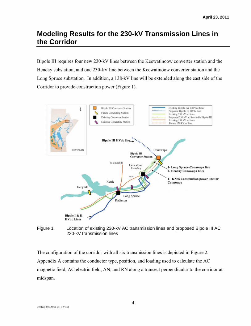
April 23, 2011
4 0704235.001 A0T0 0411 WHB5
Modeling Results for the 230-kV Transmission Lines in the Corridor
Bipole III requires four new 230-kV lines between the Keewatinoow converter station and the
Henday substation, and one 230-kV line between the Keewatinoow converter station and the
Long Spruce substation. In addition, a 138-kV line will be extended along the east side of the
Corridor to provide construction power (Figure 1).
Figure 1. Location of existing 230-kV AC transmission lines and proposed Bipole III AC 230-kV transmission lines
The configuration of the corridor with all six transmission lines is depicted in Figure 2.
Appendix A contains the conductor type, position, and loading used to calculate the AC
magnetic field, AC electric field, AN, and RN along a transect perpendicular to the corridor at
midspan.
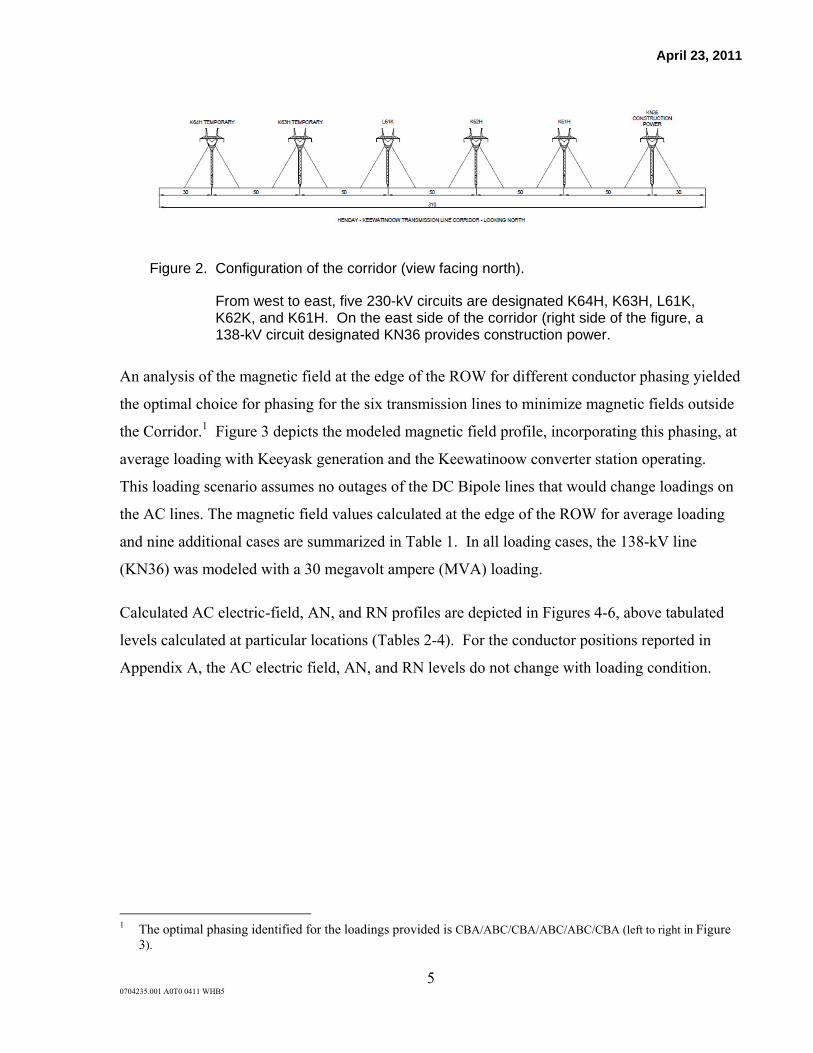
April 23, 2011
5 0704235.001 A0T0 0411 WHB5
Figure 2. Configuration of the corridor (view facing north).
From west to east, five 230-kV circuits are designated K64H, K63H, L61K, K62K, and K61H. On the east side of the corridor (right side of the figure, a 138-kV circuit designated KN36 provides construction power.
An analysis of the magnetic field at the edge of the ROW for different conductor phasing yielded
the optimal choice for phasing for the six transmission lines to minimize magnetic fields outside
the Corridor.1 Figure 3 depicts the modeled magnetic field profile, incorporating this phasing, at
average loading with Keeyask generation and the Keewatinoow converter station operating.
This loading scenario assumes no outages of the DC Bipole lines that would change loadings on
the AC lines. The magnetic field values calculated at the edge of the ROW for average loading
and nine additional cases are summarized in Table 1. In all loading cases, the 138-kV line
(KN36) was modeled with a 30 megavolt ampere (MVA) loading.
Calculated AC electric-field, AN, and RN profiles are depicted in Figures 4-6, above tabulated
levels calculated at particular locations (Tables 2-4). For the conductor positions reported in
Appendix A, the AC electric field, AN, and RN levels do not change with loading condition.
1 The optimal phasing identified for the loadings provided is CBA/ABC/CBA/ABC/ABC/CBA (left to right in Figure
3).

April 23, 2011
6 0704235.001 A0T0 0411 WHB5
Figure 3. Calculated magnetic field profile under average loading conditions with Keeyask generation and the Keewatinoow Converter Station operating.
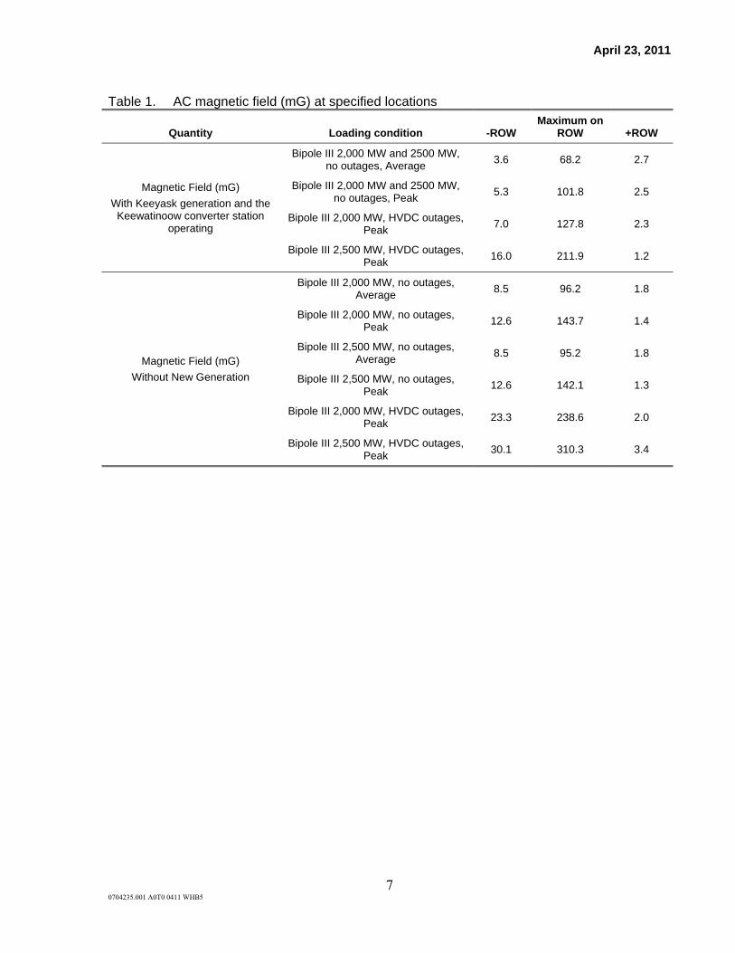
April 23, 2011
7 0704235.001 A0T0 0411 WHB5
Table 1. AC magnetic field (mG) at specified locations
Quantity Loading condition -ROW Maximum on
ROW +ROW
Magnetic Field (mG)
With Keeyask generation and the Keewatinoow converter station
operating
Bipole III 2,000 MW and 2500 MW, no outages, Average
3.6 68.2 2.7
Bipole III 2,000 MW and 2500 MW, no outages, Peak
5.3 101.8 2.5
Bipole III 2,000 MW, HVDC outages, Peak
7.0 127.8 2.3
Bipole III 2,500 MW, HVDC outages, Peak
16.0 211.9 1.2
Magnetic Field (mG)
Without New Generation
Bipole III 2,000 MW, no outages, Average
8.5 96.2 1.8
Bipole III 2,000 MW, no outages, Peak
12.6 143.7 1.4
Bipole III 2,500 MW, no outages, Average
8.5 95.2 1.8
Bipole III 2,500 MW, no outages, Peak
12.6 142.1 1.3
Bipole III 2,000 MW, HVDC outages, Peak
23.3 238.6 2.0
Bipole III 2,500 MW, HVDC outages, Peak
30.1 310.3 3.4

April 23, 2011
8 0704235.001 A0T0 0411 WHB5
Electric fields
Figure 4. Calculated AC electric field profile for the proposed cross-section in the Corridor
Table 2. Electric field (kV/m) for the transmission corridor
Quantity Loading condition -ROW Maximum on ROW +ROW
Electric Field (kV/m) Any 0.33 2.93 0.17

April 23, 2011
9 0704235.001 A0T0 0411 WHB5
Audible noise
Figure 5. Calculated AC AN profile in foul weather conditions for the proposed cross-section in the Corridor. AN under fair weather conditions will be 25 dbA lower than the levels shown above.
Table 3. Audible noise from the AC lines at specified locations under fair and foul weather
Quantity
Fair weather Foul weather
-ROW +ROW -ROW +ROW
Audible Noise (dBA) 12.1 9.0 37.1 34.0

April 23, 2011
10 0704235.001 A0T0 0411 WHB5
Radio noise
Figure 6. Calculated AC RN profile in foul weather conditions for the proposed cross-section in the Corridor calculated at 0.5 MHz. RN levels under fair weather will be 17 dBV/m lower than those shown above.
Table 4. Radio noise from the AC lines at specified locations under fair and foul weather
Quantity
Fair weather Foul weather
-15 m beyond western-most
conductor
+15 m beyond eastern-most
conductor
-15 m beyond western-most
conductor
+15 m beyond eastern-most
conductor
Radio Noise (dBV/m)
34.6 27.4 51.6 44.4

April 23, 2011
11 0704235.001 A0T0 0411 WHB5
Assessment Criteria and Conclusions
AC electric and magnetic fields
Guidelines for exposure to AC electric and magnetic fields have been recommended by ICNIRP
and the International Committee on Electromagnetic Safety (ICES) to address health and safety
issues (ICNIRP, 2010; ICES, 2002). The ICNIRP guideline limits are lower and recommended
electric field exposures less than 4.2 kV/m and magnetic field exposures less than 2,000 mG for
the general public. The levels of EMF from the new 230-kV and 138-kV transmission lines are
calculated to be well below the ICNIRP and ICES guidelines for human exposure. A review and
evaluation of current research on EMF and health relevant to exposures below these guidelines is
provided in the companion report “Research on Extremely Low Frequency Electric and
Magnetic Fields from Alternating Current Transmission Lines—Summary Evaluation of the
Evidence.” The report states:
The current consensus among the numerous national and international scientific agencies that have reviewed this extensive body of research (including the World Health Organization, the International Agency for Research on Cancer, the National Institute of Environmental Health Sciences, the Health Protection Agency of Great Britain, and the Federal-Provincial-Territorial Radiation Protection Committee of Canada) is that there is no known relationship between exposure to ELF EMF at the levels generally found in residential and occupational environments and adverse health effects. Recent research does not provide evidence to alter this conclusion.
AC audible noise
Manitoba’s Provincial Guidelines specify maximum desirable 1-hour equivalent noise levels for
residential and commercial areas of 55 dBA and 45 dBA, for day-time and night-time periods,
respectively. The median AN levels, generated by corona on the proposed 230-kV and 138-kV
transmission lines at the edge of the ROW, are estimated to be 12.1 dBA during fair weather and
37.1 dBA during foul weather, well below the Province’s AN guidelines.

April 23, 2011
12 0704235.001 A0T0 0411 WHB5
AC radio noise
The Industry Canada standard for RN for a 230-kV transmission lines is 53 dBV/m at 15 m
from the nearest conductor that would be measured by a CISPR-type measuring instrument
according to CSA Standard C108.1.1-1977 (Industry Canada, 2001). The calculated levels of
RN at 15 m from the outer conductor of the Henday to Keewatinoow K64H line is 51.6
dBV/m; at 15 m from the outermost conductor of the 138-kV circuit (KN36), on the opposite
side of the Corridor, the calculated RN level is 44.4 dBV/m. Thus, the anticipated levels of RN
associated with the operation of proposed 230-kV and 138-kV lines on this corridor are
calculated to be below the Industry Canada standard.
Conclusions
Based on the modeling of the AC Northern collector and construction power transmission lines,
the following conclusions pertain to these lines:
The levels of EMF, AN, and RN of the proposed 230-kV and 138-kV transmission lines
that will provide power to Bipole III from existing hydro-generating sources are all below
provincial, national, and international guidelines.
Further, the conclusions of these scientific agencies have been generally consistent.
Overall, they concluded that the research does not show that electric or magnetic fields
are a known or likely cause of any disease, including cancer. They also concluded that
some statistical data suggests a relationship between childhood leukemia and rare
exposure to high magnetic field levels, although the uncertainty associated with these
findings and the lack of support from experimental studies does not support a true
relationship. (Refer to Appendix B for a more detailed summary).
Although there are no residential areas close to the Northern Collector line, nevertheless,
an optimized phasing for the lines was proposed that will minimize magnetic field levels
outside the right-of-way. This no-cost action is consistent with the recommendations of
the World Health Organization (WHO, 2007).
April 23, 2011
13 0704235.001 A0T0 0411 WHB5
References
American Conference of Governmental Industrial Hygienists (ACGIH). Documentation of the Threshold Limit Values for Physical Agents. Cincinnati, OH: ACGIH, 7th Edition, 2009.
Bonneville Power Administration (BPA), USDOE. “Corona and Field Effects.” Computer Program Bonneville Power Administration, 1991.
CSA. Electromagnetic Interference Measuring Instrument – CISPR Type. Standard C108.1.1-1977, Reaffirmed 2008.
CENELEC. Human Exposure to Electromagnetic fields low-frequency (0 Hz to 10 kHz). ENV 50166-1, 1995.
Environmental Management Division, Province of Manitoba Enforcement (EMD). Guidelines for Sound Pollution. September 21, 1992.
Industry Canada. Spectrum Management and Telecommunications Policy, Interference-Causing Equipment Standard. Alternating Current High Voltage Power Systems. ICES-004, Issue 3, December, 2001.
International Commission on Non-Ionizing Radiation Protection (ICNIRP). Guidelines on limits of exposure to static magnetic fields. Health Physics 96:504-514. 2009.
International Commission on Non-Ionizing Radiation Protection (ICNIRP). ICNIRP statement—guidelines for limiting exposure to time-varying electric and magnetic fields (1 Hz to 100 kHz). Health Physics 99:818-836, 2010.
International Committee on Electromagnetic Safety (ICES). IEEE Standard for Safety Levels with Respect to Human Exposure to Electromagnetic Fields 0 to 3 kHz C95. 6-2002. Piscataway, NJ: IEEE, 2002.
Institute of Electrical and Electronics Engineers (IEEE). IEEE Standard Procedures for Measurement of Power Frequency Electric and Magnetic Fields from AC Power Lines. ANSI/IEEE Std. 0644-1994 (Revision of IEEE Standard 644-1987, Reaffirmed 2001, 2008), 1994a.
Institute of Electrical and Electronics Engineers (IEEE). IEEE recommended practice for instrumentation: specifications for magnetic flux density and electric field strength meters-10 Hz to 3 kHz. IEEE Standard 1308-1994, 1994b.
Ministry of Health of Russian Federation (MHRF). SanPin (Sanitary and Epidemiological Norms) 2.2.4. 1294-03 (New SanPin), June 16, 2003. http://www.ionization.info/issue/iss6.htm
National Radiological Protection Board (NRPB). Electromagnetic fields and the risk of cancer. Supplementary report by the Advisory Group on Non-ionising Radiation. National Radiological Protection Board. 5(2):77-81, 1994.
April 23, 2011
14 0704235.001 A0T0 0411 WHB5
National Geophysical Data Center (NGDC). 2010. Compute Earth's Magnetic Field Values. Internet website: http://www.ngdc.noaa.gov/geomag/magfield.shtml. Accessed: April, 2010.
World Health Organization (WHO). Environmental Health Criteria 238: Extremely Low Frequency (ELF) Fields. Geneva, Switzerland: World Health Organization, 2007.
.

April 23, 2011
Appendix A Input data for AC EMF, AN, and RN modeling of the Corridor

April 23, 2011
A-1 0704235.001 A0T0 0411 WHB5
Table A-1. Conductor types
Circuit Voltage
(kV) Conductor
type
Conductor diameter
(mm) Number of conductors
Conductor spacing (mm) SW type
SW diameter
(mm)
L61K 230 ACSR Drake 28.1 2 457.2 Steel
Strand 9
K61H 230 ACSR Falcon 39.2 1 0 Steel
Strand 9
K62H 230 ACSR Falcon 39.2 1 0 Steel
Strand 9
K63H 230 ACSR Falcon 39.2 1 0 Steel
Strand 9
K64H 230 ACSR Falcon 39.2 1 0 Steel
Strand 9
KN36 138 ACSR Oriole 18.8 1 0 Galvanized
Steel 9
Table A-2. Conductor locations (horizontal “x” locations measured from the west/left ROW edge)
Circuit
Conductor at mid-span [m] Shield Wire at mid-span [m]
A B C 1 2
X Y X Y X Y X Y X Y
L61K 136.7 11.1 130.0 11.1 123.3 11.1 126.9 21.9 133.1 21.9
K61H 223.3 9.6 230.0 9.6 236.7 9.6 226.9 21.9 233.1 21.9
K62H 173.3 9.6 180.0 9.6 186.7 9.6 176.9 21.9 183.1 21.9
K63H 73.3 9.6 80.0 9.6 86.7 9.6 76.9 21.9 83.1 21.9
K64H 36.7 9.6 30.0 9.6 23.3 9.6 26.9 21.9 33.1 21.9
KN36 286.7 9.1 280.0 9.1 273.3 9.1 276.9 23.4 283.1 23.4

April 23, 2011
A-2 0704235.001 A0T0 0411 WHB5
Table A-3. Loading conditions with Keeyask and the Keewatinoow converter station operating
Circuit
Bipole III 2000 MW and 2500 MW, no outages,
Average
Bipole III 2000MW and 2500 MW, no outages,
Peak Bipole III 2000MW, HVDC
outages, Peak Bipole III 2500MW, HVDC
outages, Peak
MW MVar Amps MW MVar Amps MW MVar Amps MW MVar Amps
L61K 154.77 13.40 389.96 231.00 20.00 582.03 288.00 37.00 728.88 469.00 61.00 1,187.21
K61H 58.96 4.02 148.35 88.00 6.00 221.41 117.00 11.00 294.99 280.00 16.00 704.01
K62H 58.96 4.02 148.35 88.00 6.00 221.41 117.00 11.00 294.99 280.00 16.00 704.01
K63H 58.96 4.02 148.35 88.00 6.00 221.41 117.00 11.00 294.99 280.00 16.00 704.01
K64H 58.96 4.02 148.35 88.00 6.00 221.41 117.00 11.00 294.99 280.00 16.00 704.01
KN36 29.93 2.04 125.51 29.93 2.04 125.51 29.93 2.04 125.51 29.93 2.04 125.51
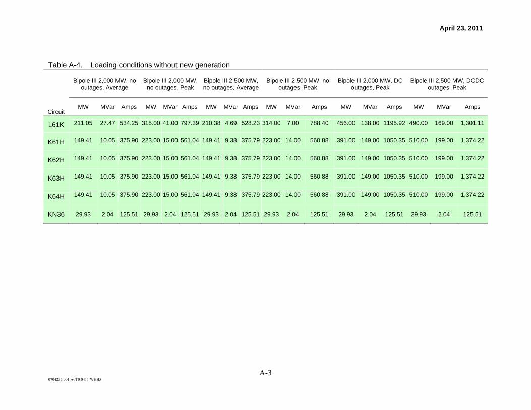
April 23, 2011
A-3 0704235.001 A0T0 0411 WHB5
Table A-4. Loading conditions without new generation
Circuit
Bipole III 2,000 MW, no outages, Average
Bipole III 2,000 MW, no outages, Peak
Bipole III 2,500 MW, no outages, Average
Bipole III 2,500 MW, no outages, Peak
Bipole III 2,000 MW, DC outages, Peak
Bipole III 2,500 MW, DCDC outages, Peak
MW MVar Amps MW MVar Amps MW MVar Amps MW MVar Amps MW MVar Amps MW MVar Amps
L61K 211.05 27.47 534.25 315.00 41.00 797.39 210.38 4.69 528.23 314.00 7.00 788.40 456.00 138.00 1195.92 490.00 169.00 1,301.11
K61H 149.41 10.05 375.90 223.00 15.00 561.04 149.41 9.38 375.79 223.00 14.00 560.88 391.00 149.00 1050.35 510.00 199.00 1,374.22
K62H 149.41 10.05 375.90 223.00 15.00 561.04 149.41 9.38 375.79 223.00 14.00 560.88 391.00 149.00 1050.35 510.00 199.00 1,374.22
K63H 149.41 10.05 375.90 223.00 15.00 561.04 149.41 9.38 375.79 223.00 14.00 560.88 391.00 149.00 1050.35 510.00 199.00 1,374.22
K64H 149.41 10.05 375.90 223.00 15.00 561.04 149.41 9.38 375.79 223.00 14.00 560.88 391.00 149.00 1050.35 510.00 199.00 1,374.22
KN36 29.93 2.04 125.51 29.93 2.04 125.51 29.93 2.04 125.51 29.93 2.04 125.51 29.93 2.04 125.51 29.93 2.04 125.51

Appendix B Exponent’s Report on EMF and Health

Health Sciences Group
Research on Extremely Low Frequency Electric and Magnetic Fields from Alternating Current Transmission Lines—Summary Evaluation of the Evidence

0704235.001 A0T0 0411 WHB5
Research on Extremely Low Frequency Electric and Magnetic Fields from Alternating Current Transmission Lines—Summary Evaluation of the Evidence Prepared for Manitoba Hydro Transmission Planning & Design 820 Taylor Avenue Winnipeg, Manitoba R3C2P4 Prepared by Exponent 17000 Science Drive Suite 200 Bowie, MD 20715 February 2011 Exponent, Inc.

0704235.001 A0T0 0411 WHB5
Notice This report summarizes work performed to-date and presents the findings resulting from that work. The findings presented herein are made to a reasonable degree of scientific certainty. Exponent reserves the right to supplement this report and to expand or modify opinions based on review of additional material as it becomes available through any additional work or review of additional work performed by others

February 25, 2011
0704235.001 A0T0 0411 WHB5
B-i
Contents
Page
Executive Summary ii
1. Introduction to Electric and Magnetic Fields 1
2. Scientific Research Process 5
3. Scientific Reviews of ELF EMF 10
4. Current Consensus on Specific Health Outcomes 13
Childhood leukemia 13
Childhood brain cancer 16
Adult brain and lymphohematopoietic cancers 17
Breast cancer 17
Neurodegenerative diseases 18
Reproductive and developmental effects 18
5. Standards and Guidelines 20
6. Precautionary Measures 22
7. Other Research Topics 24
References 25
Appendix 1—Conclusions of the WHO’s Environmental Health Criteria 238 Appendix 2—Health Canada (It’s Your Health – Electric and Magnetic Fields at Extremely Low Frequencies) Appendix 3— Relevant Epidemiology Studies Published after the WHO Report by Health Outcome

February 25, 2011
0704235.001 A0T0 0411 WHB5
B-ii
Executive Summary
Over the past 30 years, an extensive body of research has developed that addresses extremely
low frequency electric and magnetic fields (ELF EMF) and health. As described in Section 1 of
this report, ELF EMF is associated with anything that generates, transmits, or uses electricity, so
it is a ubiquitous exposure in all technologically advanced societies. As such, questions about
whether such exposure could affect our health were raised in the late 1970s, prompted by
epidemiology research that studied the relationship of cancer in children with potential exposure
to ELF EMF from nearby power lines.2 Since that time, researchers from many different
scientific disciplines have investigated this question and conducted thousands of epidemiology
and laboratory studies related to the potential effects of ELF EMF, including studies of cancer,
reproductive effects, and neurological effects, among other outcomes.
The current consensus among the numerous national and international scientific agencies that
have reviewed this extensive body of research (including the World Health Organization, the
International Agency for Research on Cancer, the National Institute of Environmental Health
Sciences, the Health Protection Agency of Great Britain, and the Federal-Provincial-Territorial
Radiation Protection Committee of Canada) is that there is no known relationship between
exposure to ELF EMF at the levels generally found in residential and occupational environments
and adverse health effects. Recent research does not provide evidence to alter this conclusion.
Despite the conclusions reached based upon this research, the public frequently expresses
concern about ELF EMF, often in the context of proposed new transmission lines. One question
that often arises is why scientists continue research if there is strong evidence of no effect.
Scientific research and the publication of study results is a constantly evolving process. The fact
that scientists have failed to identify any adverse effects of ELF EMF after extensive testing
increases the certainty that there are not any risks, or that any possible risk associated with
exposure is small. The nature of scientific investigation dictates that the possibility that ELF
EMF (or any other exposure in our environment) might have some adverse effect can never be
completely ruled out because it is impossible to prove the absence of an effect. Given the 2 Wertheimer N. and Leeper E. Electrical wiring configuration and childhood cancer. Am J Epidemiol 109:273-
284, 1979.

February 25, 2011
0704235.001 A0T0 0411 WHB5
B-iii
amount and quality of research that has been conducted thus far, however, the opinion of
scientific organizations is strong that there is not a cause-and-effect relationship.
A conclusion about any risk associated with ELF EMF is only reached by an unbiased evaluation
of the entire research database using established scientific methods. The scientific research
process and the scientific organizations that have carried out evaluations of research on ELF
EMF are highlighted in Sections 2 and 3. In Section 4, the current consensus these organizations
related to particular health outcomes, including childhood cancers (leukemia and brain cancer),
adult cancers (brain, lymphohematopoietic, and breast), neurodegenerative diseases, and
reproductive effects, is summarized. Finally, the standards and guidelines that have been
established, the precautionary measures that are recommended, and a brief review of some
additional research topics are covered in Sections 5, 6, and 7, respectively.

February 25, 2011
0704235.001 A0T0 0411 WHB5
B-1
1. Introduction to Electric and Magnetic Fields
The term “field” describes the space surrounding a particular object where the properties of that
object exert an influence—a temperature field, for example, surrounds warm objects because of
the radiating nature of heat. Electric fields and magnetic fields (EMF) surround both man-made
and natural sources.3 Man-made EMF surrounds objects that generate, transmit, or use
electricity such as power stations, transmission lines, distribution lines, the wiring in our homes
and offices, and the appliances and myriad of electronic devices used in everyday life. EMF
from these sources changes direction and intensity 60 times, or cycles, per second—a frequency
of 60 Hertz (Hz)—is, therefore, referred to as alternating current (AC) power. Research on ELF
EMF has focused primarily on AC power.4 Fields generated at these extremely low frequencies
(i.e., 30 – 300 Hz) differ significantly from the natural static fields (0 Hz) of the earth and fields
at higher frequencies characteristic of radio and television signals, microwave ovens, cellular
phones, and radar, all of which can have frequencies up to billions of Hz.
Electric fields are the result of voltages applied to electrical conductors and equipment. The
electric field is expressed in measurement units of volts per meter (V/m) or kilovolts per meter
(kV/m), where 1 kV/m is equal to 1,000 V/m. Most objects including fences, shrubbery, and
buildings easily block electric fields. Therefore, certain appliances within homes and the
workplace are the major sources of electric fields indoors, while power lines are the major
sources of electric fields outdoors (Figure 1, lower panel).
Magnetic fields are produced by the flow of electric currents. Unlike electric fields, most
materials do not readily block magnetic fields. The strength of magnetic fields is commonly
expressed as magnetic flux density in units of gauss (G) or milligauss (mG), where 1 G is equal
3 Natural sources of electric fields occur in the earth’s atmosphere, most commonly experienced during
thunderstorms. Although it differs from the magnetic fields generated by AC electricity because it is static, the earth’s geomagnetic field is the dominant natural source of magnetic fields. The intensity of the geomagnetic field varies with latitude; the lowest values (~ 300 mG) are measured near the equator and higher values (up to ~700 mG) are measured near the north and south poles.
4 Throughout the world, AC transmission is a more common means of power distribution than direct current (DC) or static transmission, which is used primarily for transmission of power across very long distances. For this reason, research has focused on the effects of AC EMF.

February 25, 2011
0704235.001 A0T0 0411 WHB5
B-2
to 1,000 mG.5 The strongest sources of AC magnetic fields that we encounter indoors are
electrical appliances (Figure 1, upper panel).
Figure 7. Typical exposure potentials to electric and magnetic fields in common environments.
The level of EMF produced by these sources depends on their structure, location, and various
operating characteristics; the magnetic field level produced by a particular power line, for
5 Scientists more commonly refer to magnetic flux density at lower levels in units of microtesla (µT). Magnetic
flux density in milligauss units can be converted to µT by dividing by 10, i.e., 1 mG = 0.1 µT.

February 25, 2011
0704235.001 A0T0 0411 WHB5
B-3
example, depends on the configuration of its conductors, their height from the ground, and the
amount of current running through the line, among other things.
The strength of both electric fields and magnetic fields decreases with distance from the source.
Thus, personal exposure to EMF from a particular object depends largely on a person’s distance
from that object. While appliances tend to produce the highest levels of magnetic fields in our
home and work environments, the magnetic fields from appliances drop off more quickly with
distance than other EMF sources. 6
Every individual has an “average” EMF exposure level that is defined by the environments
where they spend time, the sources encountered in those locations, and the duration of exposure
to these sources. If any of these variables change, the person’s average exposure may be altered.
Occupation as a welder or railway worker, for example, would elevate a person’s average EMF
exposure for the duration of that employment; or, if a person lived in a home with faulty wiring,
his or her average EMF exposure may be elevated during that period. Background levels of
magnetic fields (estimated from an average of measurements taken throughout a typical home
away from appliances) range from 1-2 mG, while background levels of electric fields range from
0.01-0.02 kV/m; however, in proximity to appliances, magnetic field levels can be hundreds of
times higher and electric field levels tens of times higher, as illustrated in Figure 1 (Savitz et al.,
1989; WHO, 2007). The ubiquitous nature of EMF and variability in average exposure levels
make it difficult to quantify levels of exposure for research studies. As a result, the major
limitation of health studies of EMF is the methods used for estimating exposure.
Data from Canada show that persons are exposed to daily average levels of approximately 1 mG
(Armstrong et al., 2001). The average magnetic-field exposures of American children are similar
(Zaffanella, 1998). Figure 2 below displays data from measurements taken by a gaussmeter
worn by a person for a 48-hour period while conducting ordinary activities at home, at work, and
in between (i.e., driving and riding the train). These measurements illustrate the continuous but
varying levels of magnetic fields that most people encounter each day. Even though high levels
6 Fields near appliances vary over a wide range, from a fraction of 1 mG to 1,000 mG or more. Gauger (1985)
reported the maximum AC magnetic field at 3 centimeters from a sampling of appliances as 3,000 mG (can opener), 2,000 mG (hair dryer), 5 mG (oven), and 0.7 mG (refrigerator).

0704235.001 A0T
of exposu
brief. Av
Figure 8.
T0 0411 WHB5
ure were com
verage expos
. Magn
Source
mmon and th
sure over the
netic field exp
e: Exponent (20
he highest le
ese two days
posure over
007)
B-4
evel reached
s was just a f
the course o
168 mG, su
fraction over
of a 48-hour
F
uch high expo
r 1 mG.
period.
February 25,
osures were
, 2011

February 25, 2011
0704235.001 A0T0 0411 WHB5
B-5
2. Scientific Research Process
Scientific inquiry is not simply a collection of facts – it is a systematic and unbiased reasoning
process used to arrive at accurate and balanced conclusions. The scientific process must,
therefore, be conducted in a manner to ensure that conclusions are supported by the research.
Many misconceptions in human reasoning occur, for example, when casual observations are
made about a particular experience (for example, if a person develops a headache after eating a
particular food, he or she may ascribe the headache to the food). Proximity of events or
conditions, however, does not guarantee a causal relationship. The same mistake can occur
when conclusions are based on the results of single studies. Scientists use systematic methods to
evaluate observations and assess the potential impact of a specific agent on human health.
The scientific process involves looking at all the evidence on a particular issue in a systematic
and thorough manner, an evaluation that is often referred to as a weight-of-evidence review.
This process is designed to ensure that more weight is given to studies of better quality and that
studies with a given result are not selected from the available evidence to advocate or suppress a
preconceived hypothesis. Conclusions about health risks cannot be drawn from single studies
because every study has limitations in one way or another. A weight-of-evidence review is
based on a comprehensive assessment of the three main types of scientific research (Figure 3):
epidemiology studies of humans; experimental studies in animals (in vivo); and experimental
studies in isolated cells and tissues (in vitro).

February 25, 2011
0704235.001 A0T0 0411 WHB5
B-6
Figure 9. Study types included in a weight-of-evidence
review
A weight-of-evidence review first evaluates individual studies in terms of their strengths and
weaknesses and then evaluates all of the studies together, taking the appropriate pieces of
evidence from each study to form a conclusion. In this process, the information provided by
epidemiology and in vivo studies is complementary. Epidemiology studies are limited by the
lack of control they have over their study participants, but provide information directly relevant
to the species of interest; the results from in vivo studies, while often more accurate because of
the experimental nature of the study, need to be extrapolated to what would be expected in
humans. Thus, the overall patterns of results from epidemiology and in vivo studies are
considered because epidemiology studies address the limitations of in vivo studies and vice
versa.7
Each study contributes a different type and weight of evidence due to the inherent qualities of its
study design, the methods used in collecting and analyzing the data, and any biases that may
have arisen during the course of the study. A high-quality epidemiology study, for example,
would consist of a large cohort of a highly-exposed population with follow-up of all its study
participants over a long period of time with detailed measurements of exposure for each study
participant during the relevant periods of exposure. This study design is expensive and time-
7 The findings of in vitro studies are used by health and regulatory agencies to help them interpret the results of in
vivo studies, but in vitro studies may not be representative of the response to the agent of interest. These agencies, therefore, do not directly rely on in vitro studies to make policy decisions.
The data from all three study types should be considered in evaluating health risks

February 25, 2011
0704235.001 A0T0 0411 WHB5
B-7
consuming; thus, other study types (e.g., the case-control design) and dosimetric methods (e.g.,
job-exposure matrices) are used with a full understanding of their limitations.
The main result of an epidemiology study is the statistical association measured between the
exposure and disease of interest. When evaluating any study, it is important to consider that its
results do not represent the real relationship between an exposure and a disease; rather, the
results represent some estimation of the relationship in a single population, which is limited by
the study’s methods and, in the case of epidemiology studies, the unpredictable behavior of the
study’s participants. In fact, much of epidemiologic analysis involves the interpretation of how
outside factors could have affected the study’s statistical findings.
Statistical associations in cohort studies are summarized by a computed relative risk, which is a
ratio of the risk of the disease in the exposed group to the ratio of the risk in the unexposed
group. A value greater than 1.0 indicates a positive association and a possible risk associated
with exposure. Case-control studies estimate relative risks with an odds ratio, which is a ratio of
the odds of exposure among persons with a disease (i.e., cases) to the odds of exposure among a
similar population without disease (i.e., controls).
Three factors are always considered when evaluating the weight assigned to any statistical
association:
1. Chance. A statistical association may simply be due to a chance occurrence.
Statistical tests are performed to evaluate whether chance is a likely explanation.
2. Bias. Bias is any systematic error in the design, implementation, or analysis of a
study that results in a mistaken estimate of an exposure’s effect on the risk of disease.
Bias can occur, for example, if a study compares disease rates of exposed and
unexposed groups comprised of persons in different age groups.
3. Confounding. A confounder is something that is related to both the disease under
study and the exposure of interest such that one cannot be sure what causes the
observed association—the confounder or the exposure of interest. With regard to
epidemiology studies of EMF from distribution lines and childhood cancer, some

February 25, 2011
0704235.001 A0T0 0411 WHB5
B-8
scientists have investigated whether the association is confounded by exposures to
emissions from vehicles on adjacent roadways.
Scientific diligence and care must be taken in the design and analysis of studies to evaluate the
role of chance and minimize bias and confounding so these factors do not distort the study’s
findings.
Scientific panels often classify epidemiologic data as providing sufficient, limited, inadequate
evidence in support of carcinogenicity (i.e., the ability of an agent to cause cancer), or evidence
suggesting a lack of carcinogenicity, using the standardized classification process established by
the International Agency for Research on Cancer (IARC). For the evidence to be considered
sufficient, the role of chance, bias, and confounding on the observed association must be ruled
out with “reasonable confidence.” If the role these factors may play in the calculated statistical
association cannot be ruled out with reasonable confidence, then the data is classified as
providing limited evidence. Inadequate evidence describes a data set that lacks quality,
consistency, or power for conclusions regarding causality to be drawn. This classification
system is used for both epidemiology studies and in vivo studies and is used to provide summary
descriptions of an exposure’s potential to cause cancer – known carcinogens, probable
carcinogens, possible carcinogens, not classifiable, and probably not a carcinogen (as illustrated
in Figure 4).

February 25, 2011
0704235.001 A0T0 0411 WHB5
B-9
Figure 10. IARC method for classifying exposures according to carcinogenicity

February 25, 2011
0704235.001 A0T0 0411 WHB5
B-10
3. Scientific Reviews of ELF EMF
Multidisciplinary scientific panels of both international and national scientific and governmental
agencies regularly conduct weight-of-evidence reviews about possible health risks—it is these
evaluations and the conclusions stemming from them that guide research priorities and help set
standards and guidelines to reduce potential exposure risks. Numerous weight-of-evidence
reviews of the research literature on ELF EMF and possible adverse health effects have been
conducted by and national scientific and governmental agencies. The major agencies that have
reviewed this topic are listed below in Table 1, with their most recent weigh-of-evidence review
indicated.
Table 5. Weight-of-evidence and other major reviews, 1998 - 2010 Year Agency Publication
1998 National Institute for Environmental Health Sciences (NIEHS)
Assessment of health effects from exposure to power-line frequency electric and magnetic fields: working group report
1998, updated in
2005
Federal-Provincial-Territorial Radiation Protection Committee (FPTRPC)
Health effects and exposure guidelines related to extremely low frequency electric and magnetic fields—an overview
2002 International Agency for Research on Cancer (IARC)
IARC monographs on the evaluation of carcinogenic risks to humans. Volume 80: Static and extremely low-frequency (ELF) electric and magnetic fields
2004
National Radiological Protection Board of Great Britain (NRPB)
Currently known as the Health Protection Agency [HPA] of Great Britain
Review of the scientific evidence for limiting exposure to electromagnetic fields (0-300 GHz). Volume 15, No. 3
2007 World Health Organization (WHO) Environmental Health Criteria 238: Extremely low frequency (ELF) Fields
2008 Swedish Radiation Protection Agency (SSI)
Fifth Annual report from SSI’s Independent Expert Group on electromagnetic fields, 2007: Recent research on EMF and health risks
2009 Scientific Committee on Emerging and Newly Identified Health Risks (SCENIHR)
Health effects of exposure to EMF
2010 ICNIRP ICNIRP Statement—Guidelines for limiting exposure to time-varying electric and magnetic fields (1 Hz to 100 KHz)
None of these agencies has concluded that exposure to ELF EMF is a demonstrated cause of any
long-term adverse health effect. Section 4 describes the current scientific evidence with regard
to specific health outcomes. The evidence in support of a causal relationship is weak because it
is founded largely, if not entirely, on some epidemiology studies that reported statistical

February 25, 2011
0704235.001 A0T0 0411 WHB5
B-11
associations between higher estimated average magnetic field exposure and a disease. Overall,
the in vivo studies did not report an increase in cancer among animals exposed to high levels of
electric or magnetic fields, and in vitro studies have not confirmed a mechanism that would
explain how electric or magnetic fields could initiate disease.
Most notably, a weak statistical association was reported between childhood leukemia and
estimates of long-term exposure to high average magnetic field levels (3-4 mG). The overall
body of research, however, does not indicate that this association, or any other, is causal in
nature. Weaknesses in the epidemiology studies of childhood leukemia limit the significance of
their findings; specifically, scientists have not been able to rule out the possibility that
confounding or bias contributes to the statistical association between magnetic fields and
childhood leukemia reported in these studies. Furthermore, findings from in vivo and in vitro
studies do not support a causal relationship.
The only studies that can be said to confirm a relationship between electric fields or magnetic
fields and an adverse biological or health effect are those in which very high levels of exposure
to these fields produce currents and fields in the body, which can result in a shock-like effect.
The levels at which these short-term effects occur are very high and may not even be reached in
high exposure occupational environments. Several organizations have recommended exposure
guidelines to protect against their occurrence. These guidelines are summarized in Section 5.
The conclusions of the most extensive of these scientific reviews—the WHO review—, which
were published in 2007, are summarized in Appendix 1. Several scientific organizations have
recently released reports or statements of note related to ELF EMF. When ICNIRP prepared
revised guidelines for ELF EMF exposure, which were released in December 2010, they also
reviewed the evidence related to long-term health effects, and they concluded the following:
The literature on chronic effects of ELF fields has been evaluated in detail
by individual scientists and scientific panels. WHO’s cancer research
institute, IARC (International Agency for Research on Cancer) evaluated
ELF magnetic fields in 2002 and classified them in category 2B, which
translates to “possibly carcinogenic to humans.” The basis for this
classification was the epidemiologic results on childhood leukemia. It is

February 25, 2011
0704235.001 A0T0 0411 WHB5
B-12
the view of ICNIRP that the currently existing scientific evidence that
prolonged exposure to ELF magnetic fields is causally related with an
increased risk of childhood leukemia is too weak to form the basis for
exposure guidelines (ICNIRP 2010, p. 824).
The FPTRPC of Canada released a statement in November 2008 that concluded the following
with respect to EMF and health:
In summary, it is the opinion of the Federal-Provincial-Territorial
Radiation Protection Committee that there is insufficient scientific
evidence showing exposure to EMFs from power lines can cause adverse
health effects such as cancer.
This conclusion is consistent with statements by Health Canada in their publication “It’s Your
Health—Electric and Magnetic Fields at Extremely Low Frequencies,” which were updated in
January 2010. Specifically, they state, “In summary, when all of the studies are evaluated
together, the evidence suggesting that EMFs may contribute to an increased risk of cancer is very
weak.” This publication can be found on Health Canada’s website and is also included in
Appendix 2.8
The following section reviews the current consensus of these organizations related to particular
health outcomes, including childhood cancers (leukemia and brain cancer), adult cancers (brain,
lymphohematopoietic, and breast), neurodegenerative diseases, and reproductive effects. For
reference Appendix 3 provides a listing of epidemiology studies published since the time of the
WHO 2007 review.
8 http://www.hc-sc.gc.ca/hl-vs/iyh-vsv/environ/magnet-eng.php

February 25, 2011
0704235.001 A0T0 0411 WHB5
B-13
4. Current Consensus on Specific Health Outcomes
Childhood leukemia
The incidence rate of leukemia in children is approximately 3 per 100,000 per year, making it a
relatively rare cancer, and in the vast majority of cases, the cause is unknown. The only
identified causes of childhood leukemia include certain genetic diseases, chemotherapeutic
agents, and ionizing radiation from sources such as maternal x-rays during pregnancy, but these
account for only a very small percentage of cases. Since so little is known about the cause of this
disease, many exposures have been investigated, including infectious agents and environmental
exposures such as pesticides, solvents, pollution, and magnetic fields, but no clear patterns have
emerged. Suggestive data exists for the role of infections in promoting leukemia in already
susceptible children, but the research is inadequate so conclusions about this possible cause are
not definitive.
Since 1979, epidemiology studies conducted in the United States, Canada, Europe, New Zealand,
and Asia have evaluated the relationship between childhood leukemia and some proxy of
magnetic field exposure. Independently, these studies did not show a clearly consistent
association between magnetic fields and childhood leukemia. The largest and most
methodologically sound case-control studies in this group that directly estimated magnetic field
exposure through long-term personal measurements were conducted by Linet et al. (1997) in the
United States, McBride et al. (1999) in Canada, and the United Kingdom Childhood Cancer
Study Investigators in the UK (UKCCS, 1999, 2000). None of the investigator who performed
these studies concluded that their data showed a causal relationship between childhood leukemia
and magnetic fields.

February 25, 2011
0704235.001 A0T0 0411 WHB5
B-14
A 2-fold statistically-significant association was observed between magnetic fields and
childhood leukemia when two independent pooled analyses combined the data from most of the
case-control studies published prior to 2000; this association was only observed at rare average
magnetic field exposure levels above 3-4 mG (Ahlbom et al., 2000; Greenland et al., 2000).9 As
a result of the findings by Ahlbom et al. and Greenland et al., the IARC and WHO concluded
that there is a statistical association between magnetic fields and childhood leukemia.
Researchers have not concluded, however, that the weak association between childhood
leukemia and magnetic fields is causal in nature because the studies are of insufficient quality to
rule out the role that chance, bias (e.g., exposure misclassification), and confounding may have
on the observed statistical association with “reasonable confidence.” As described in Section 2,
statistical associations are a measure of how disease and exposure estimates vary together in a
specific population, but do not indicate that two factors are causally related. Conclusions about
causality are made only when strong epidemiologic data are consistent with the data from in vivo
research, and the studies that present such data have confidently ruled out that chance, bias, or
confounding played a role in the statistical association. In their 2007 report, the WHO concluded
that, while chance is an unlikely explanation, bias arising from uncertainties in exposure (i.e.,
misclassification) and non-participation of highly-exposed controls (i.e., selection bias) is likely.
Although the WHO report (2007) identified confounding as an unlikely explanation for the
statistical association, the reviewers could not rule out its influence because so little is known
about the causes of childhood leukemia. Since transmission line right-of-ways are often built
along highways, children who live near power lines may also be likely to live near highways. If
pollutants from traffic emissions were a cause of childhood leukemia, the association between
residential distance to power lines and childhood leukemia could be the result of pollutants from
traffic, not magnetic fields from transmission lines. While this is a plausible theory, the research
on traffic emissions and childhood leukemia is inconsistent and weak.
9 Pooled and meta-analyses combine data from original studies to calculate a summary estimate of the association.
Pooled analyses combine the actual raw data, while meta-analyses combine the measures of association. The results indicate that children with leukemia were about two times more likely to have had estimated average magnetic field exposures above 3-4 mG.

February 25, 2011
0704235.001 A0T0 0411 WHB5
B-15
Approximately 18 studies related to childhood leukemia have been published between 2006 and
2010, but these have failed to explain the statistical association between estimates of high
average exposure to magnetic fields (i.e., greater than 3-4 mG) and childhood leukemia.10 Most
notably, Kheifets et al. (2010) conducted a pooled analysis of studies published between 2000
and 2010 that was intended to mirror the earlier pooled analyses of studies published between
1974 and 1999 (Ahlbom et al., 2000; Greenland et al., 2000). Kheifets et al. identified six
studies for the main analysis that met their inclusion criteria (i.e., population-based studies of
childhood leukemia that measured or calculated magnetic fields inside a home). A large number
of cases were identified by Kheifets et al. (10,865), but a relatively small number of cases (23)
were classified in the highest exposure category (>3 mG). A positive association was reported
(OR=1.44), but it was weaker than the previous pooled estimates and not statistically significant
(95% CI=0.88–2.36); a non-significant dose-response relationship was described.
No studies have replicated the statistical association between childhood leukemia and average
personal exposure greater than 3-4 mG, although recent studies have reported associations of
magnetic fields with poor health outcomes at estimates of elevated magnetic field levels.
Specifically, these studies reported that children with leukemia and estimates of elevated average
magnetic field exposures had poorer survival rates; children with Down’s syndrome and
childhood leukemia were more likely to have an estimated magnetic field exposure greater than 6
mG; and children with leukemia and a genetic variation associated with a reduced ability to
repair DNA were more likely to live closer to an electrical installation. None of the studies,
however, is methodologically strong.
Recent studies have also reported an association between higher calculated magnetic fields from
nearby power lines and childhood leukemia. Like the studies reviewed by the WHO, these
studies have limitations that preclude any clear interpretation. Furthermore, the studies tested
new hypotheses without supporting biological evidence and, therefore, require replication. Thus,
reviews of these newer studies by the Swedish Radiation Protection Authority and the Scientific
Committee on Emerging and Newly Identified Health Risks have not concluded that they
strengthen the weight of evidence for an association of magnetic fields and childhood leukemia
(SCENIHR, 2009; SSI, 2007, 2008). 10 A table of epidemiology studies published after the WHO report is included in Appendix 3.

February 25, 2011
0704235.001 A0T0 0411 WHB5
B-16
As suggested by the WHO report, methodological research has recently been conducted to
determine the role that confounding or control selection bias may have on the observed
association. 11 Findings suggest that control selection bias is operating to some extent. More
research is required to further evaluate the role of control selection bias and confounding.
None of these recent studies are sufficiently strong methodologically, nor do the findings display
causal patterns (i.e., exposure-response, consistency, and strength) to alter previous conclusions
that the epidemiologic evidence related to magnetic fields and childhood leukemia is limited.
Chance, confounding, and several sources of bias cannot be ruled out as an explanation for the
observed statistical association. The lack of evidence from recent in vivo research supports this
conclusion.
Childhood brain cancer
Similar to childhood leukemia, the causes of childhood brain cancer are relatively unknown.
Only two causes—radiotherapy for the treatment of other cancers and a particular genetic
mutation—have been identified. Far fewer studies have been published on magnetic fields and
childhood brain cancer than studies on childhood leukemia. The WHO report described the
results of these studies as inconsistent and limited by small sample size and recommended that a
meta-analysis of the data related to childhood brain cancer and magnetic field exposure be
performed.
Five studies have been published on childhood brain cancer and EMF since the time of the WHO
report. The meta- and pooled analyses conducted in response to the WHO’s recommendation
reported a very weak association between estimated average exposures greater than 3-4 mG and
childhood brain cancer, although the association was not statistically significant (i.e., not
distinguishable from chance). The authors concluded that the analyses provide little evidence for
a relationship between magnetic fields and childhood brain cancer. Recent studies on the risk of
11 Control selection bias refers to a particular type of bias that occurs in case-control studies. If the characteristics
of the control group differ from the characteristics of the case group in a way that is related to exposure, the measured statistical association will not represent a true relationship. In the case of magnetic fields and childhood leukemia, researchers are concerned that, because of factors that affect participation in a study, the control group may have a higher socio-economic status than the case group and, as a result, lower magnetic field exposures.

February 25, 2011
0704235.001 A0T0 0411 WHB5
B-17
childhood brain cancer related to pre- and post-conception parental ELF EMF exposure do not
provide strong evidence of a risk and add little to the existing body of inconsistent literature in
this area. Thus, the evidence related to childhood brain cancer and magnetic field exposure
remains inadequate.
Adult brain and lymphohematopoietic cancers
The WHO and other agencies previously classified studies of these cancer types as inadequate,
weak, and seriously limited by methods used for exposure assessment. Twelve recent studies
have reported data on adult leukemia, brain cancer and/or lymphoma. Recent studies have
reduced possible exposure misclassification by improving exposure assessment methods and
attempted to clarify inconsistencies by updating studies and meta-analyzing data; however,
despite these advancements, no consistent association has been observed. A meta-analysis was
conducted as recommended in the WHO report, which reported a small and statistically
significant increase of leukemia and brain cancer in relation to the highest estimate of magnetic-
field exposure in the individual studies (Kheifets et al., 2008). Several findings, however, led the
authors to conclude that magnetic field exposure is not likely to be responsible for the observed
associations. While an association cannot be entirely ruled out because of the remaining
deficiencies in exposure assessment methods, the current database of studies provides weak
evidence of an association between magnetic fields and adult brain and lymphohematopoietic
cancers.12
Breast cancer
The WHO concluded that there was strong evidence in support of no relationship between
magnetic fields and breast cancer; six recent studies, including one large cohort study, support
this conclusion.
12 A recent consensus statement by the National Cancer Institute’s Brain Tumor Epidemiology Consortium
confirms this statement. They classified residential power frequency EMF in the category “probably not risk factors” and described the epidemiologic data as “unresolved” (p. 1958, Bondy et al., 2008).

February 25, 2011
0704235.001 A0T0 0411 WHB5
B-18
Neurodegenerative diseases
The research on ELF EMF and neurodegenerative diseases such as Alzheimer’s disease and
amyotrophic lateral sclerosis (ALS), also known as Lou Gehrig’s disease, did not begin until
around 1995, later than other areas of ELF EMF research. The WHO report stated that there is
inadequate data in support of an association between magnetic fields and either of these two
diseases. Alzheimer’s disease, in particular, presents a unique challenge to epidemiologists
because of the nature of the disease. Disease onset is typically late in life and is difficult to
define because it is often preceded by a period of dementia, which can be misdiagnosed as other
neurodegenerative conditions, such as cerebrovascular disease. Misclassification of disease is,
therefore, common and the since the disease may be present well before symptoms appear, the
etiologically relevant time period used to make estimates of exposure may be incorrect.
Six studies have been published since the WHO report was released that addressed magnetic
field exposure and neurodegenerative diseases. While most recent studies and a meta-analysis
reported an association between occupational magnetic field exposure and Alzheimer’s disease
or ALS, the studies are weak in design, meaning the data in support of a causal relationship is
still limited. The first study that investigated non-occupational exposure was published recently,
reporting that persons living close to high-voltage transmission lines were more likely to have
died from Alzheimer’s disease than persons living at a distance from these lines. These findings
do not provide strong evidence in support of a relationship between Alzheimer’s disease and
EMF, however, mainly because distance is not a good proxy for magnetic-field exposure.
The recent epidemiology studies do not alter the conclusion that there is “inadequate” data on
Alzheimer’s disease and ALS. While a good number of studies have been published since the
WHO report, little progress has been made on clarifying these associations. Further research is
still required, particularly on electrical occupations and ALS. There is currently no body of in
vivo research to suggest an effect.
Reproductive and developmental effects
Very little epidemiologic research has been published in this area. The WHO categorized this
data as inadequate, stating that there is some evidence in support of peak magnetic-field

February 25, 2011
0704235.001 A0T0 0411 WHB5
B-19
exposures and miscarriage, but there were methodological issues with this research. The results
from two recently published studies support the role of bias in the studies of peak magnetic-field
exposure and miscarriage. There continues to be no convincing epidemiologic evidence linking
magnetic field exposure to the risk of miscarriage.

February 25, 2011
0704235.001 A0T0 0411 WHB5
B-20
5. Standards and Guidelines
Since the scientific organizations that regularly review research on ELF EMF have determined
there are no known long-term health effects from exposure, no standards or guidelines limiting
exposure to ELF EMF based on long-term health effects have been recommended. Accordingly,
there are no national standards in Canada or the United States limiting exposures to ELF EMF
based on long-term or other health effects.
Two of the scientific organizations that review the scientific literature on ELF EMF (ICNIRP
and the International Commission on Electromagnetic Safety [ICES]) have published guidelines
limiting exposure to very high levels of ELF EMF based on the avoidance of immediate short-
term health effects, which include biological responses such as perception, annoyance, and the
stimulation of nerves and muscles. Following a thorough review of the scientific literature
related to short- and long-term adverse effects, the ICNIRP published revised guidelines in
December 2010 to replace their 1998 ELF EMF guidelines. The document recommended no
change to ICNIRP’s assessment of the scientific evidence; as before, research related to long-
term health effects does not provide sufficient evidence to warrant a change to the exposure
guidelines. ICNIRP did, however, raise the residential screening value for magnetic fields from
833 to 2,000 mG. The occupational screening value of 4,200 mG (ICNIRP, 1998; ICNIRP,
2010) was not changed.
The ICES also recommends limiting exposures at high levels because of the risk of immediate
stimulation responses, although their guidelines are set well above ICNIRP’s guidelines (ICES,
2002). 13 In almost all cases, transmission lines meet these magnetic-field exposure guidelines,
although some appliances do not.
13 The ICES is “responsible for development of standards for the safe use of electromagnetic energy in the range of
0 Hz to 300 GHz relative to the potential hazards of exposure of humans, volatile materials, and explosive devices to such energy, standards for products that emit electromagnetic energy by design or as a by-product of their operation, and standards for environmental limits.”

February 25, 2011
0704235.001 A0T0 0411 WHB5
B-21
Table 6. Reference levels for whole body exposure to 60-Hz fields: general public
Organization recommending limit Magnetic
fields Electric fields
ICNIRP restriction level 2,000 mG 4.2 kV /m
ICES maximum permissible exposure (MPE) 9,040 mG 5 kV/m
10 kV/ma a This is an exception within transmission line rights of way (ROW) because people do not spend a
substantial amount of time in ROWs and very specific conditions are needed before a response is likely to occur (i.e., a person must be well insulated from ground and must contact a grounded conductor).
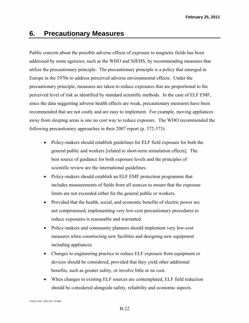
February 25, 2011
0704235.001 A0T0 0411 WHB5
B-22
6. Precautionary Measures
Public concern about the possible adverse effects of exposure to magnetic fields has been
addressed by some agencies, such as the WHO and NIEHS, by recommending measures that
utilize the precautionary principle. The precautionary principle is a policy that emerged in
Europe in the 1970s to address perceived adverse environmental effects. Under the
precautionary principle, measures are taken to reduce exposures that are proportional to the
perceived level of risk as identified by standard scientific methods. In the case of ELF EMF,
since the data suggesting adverse health effects are weak, precautionary measures have been
recommended that are not costly and are easy to implement. For example, moving appliances
away from sleeping areas is one no cost way to reduce exposure. The WHO recommended the
following precautionary approaches in their 2007 report (p. 372-373):
Policy-makers should establish guidelines for ELF field exposure for both the
general public and workers [related to short-term stimulation effects]. The
best source of guidance for both exposure levels and the principles of
scientific review are the international guidelines.
Policy-makers should establish an ELF EMF protection programme that
includes measurements of fields from all sources to ensure that the exposure
limits are not exceeded either for the general public or workers.
Provided that the health, social, and economic benefits of electric power are
not compromised, implementing very low-cost precautionary procedures to
reduce exposures is reasonable and warranted.
Policy-makers and community planners should implement very low-cost
measures when constructing new facilities and designing new equipment
including appliances.
Changes to engineering practice to reduce ELF exposure from equipment or
devices should be considered, provided that they yield other additional
benefits, such as greater safety, or involve little or no cost.
When changes to existing ELF sources are contemplated, ELF field reduction
should be considered alongside safety, reliability and economic aspects.

February 25, 2011
0704235.001 A0T0 0411 WHB5
B-23
Local authorities should enforce wiring regulations to reduce unintentional
ground currents when building new or rewiring existing facilities, while
maintaining safety. Proactive measures to identify violations or existing
problems in wiring would be expensive and unlikely to be justified.
National authorities should implement an effective and open communication
strategy to enable informed decision-making by all stakeholders; this should
include information on how individuals can reduce their own exposure.
Local authorities should improve planning of ELF EMF-emitting facilities,
including better consultation between industry, local government, and citizens
when siting major ELF EMF-emitting sources.
Government and industry should promote research programmes to reduce the
uncertainty of the scientific evidence on the health effects of ELF field
exposure.
In Canada, the FPTRPC’s approach to precautionary measures is similar to the recommendations
made by the WHO. The FPTRPC stated, “In the context of power-frequency EMFs, health risks
to the public from such exposures have not been established; therefore, it is the opinion of the
FPTRPC that any precautionary measures applied to power lines should favour low cost or no
cost options.”

February 25, 2011
0704235.001 A0T0 0411 WHB5
B-24
7. Other Research Topics
High-voltage and ultra-high-voltage transmission lines often traverse farmland, forests, and
woodlands that have substantial populations of both domestic and wild animals and a wide
variety of crops and plants. Prompted by concerns about the effects of EMF through these areas,
research has been conducted since the 1970s on the possible effects of EMF on the health,
behavior, and productivity of a number of species, including livestock and a range of wild
animals and insects, as well as the possible effects on farm crops and natural flora. The research
to date does not suggest that magnetic or electric fields (or any other aspect of high-voltage
transmission lines, such as audible noise) result in adverse effects on the health, behavior, or
productivity of fauna, including livestock such as dairy cows, sheep, pigs, and a variety of other
species including small mammals, deer, elk, birds, and bees. Studies were also conducted to
evaluate whether EMF could affect crops or plants, but did not suggest any adverse effects on
growth or viability.
Another area of concern that has been raised in relation to EMF exposure is the effects of these
fields on pacemakers or implanted cardiac devices (ICDs). The heart’s rhythm is controlled
naturally by electrical signals. When there is a disturbance to this rhythm, a pacemaker or ICD is
implanted to restore normal cardiac function. Since the sensing system of these devices is
naturally responsive to the heart’s electrical signal, other electrical signals can interfere with the
normal functioning of pacemakers and ICDs, a phenomenon called electromagnetic interference
(EMI). Potential sources of EMI include cellular telephones, anti-theft devices in stores, MRI
machines, slot machines, and certain medical procedures (e.g., radiation therapy, electrocautery,
and defibrillation). Experimental tests have shown sometimes subtle effects of strong electric
fields on pacemaker operation, but no case reports of interference with patients’ pacemakers by
electric or magnetic fields associated with transmission lines have been reported in the literature.
Transmission line magnetic fields are generally too weak to affect pacemakers, and electric field
strength decreases with distance and is shielded by trees, buildings, vehicles, fences, etc. Most
devices are now constructed with features that prevent interference.

February 25, 2011
0704235.001 A0T0 0411 WHB5
B-25
References
Ahlbom A, Day N, Feychting M, Roman E, Skinner J, Dockerty J, Linet M, Michealis J, Olsen JH, Tynes T, Verkasalo PK. A pooled analysis of magnetic fields and childhood leukemia. Br J Cancer 83:692-698, 2000.
Armstrong BG, Deadman J, McBride ML. The determinants of Canadian children’s personal exposure to magnetic fields. Bioelectromagnetics 22:161-169, 2001.
Federal-Provincial-Territorial Radiation Protection Committee. Health effects and exposure guidelines related to extremely low frequency (ELF) 50/60 Hz electric and magnetic fields – an overview. Prepared by the ELF Working Group, 1998.
Federal-Provincial-Territorial Radiation Protection Committee. Heath Effects and Exposure Guidelines Related to Extremely Low Frequency Electric and Magnetic Fields - An Overview. Prepared by The ELF Working Group, 2005.
Federal-Provincial-Territorial Radiation Protection Committee (FPTRPC). Response Statement to Public Concerns Regarding Electric and Magnetic Fields (EMFs) from Electric Power Transmission and Distribution Lines. November 8, 2008. http://www.hc-sc.gc.ca/ewh-semt/radiation/fpt-radprotect/emf-cem-eng.php)
Greenland S, Sheppard AR, Kelsh MA, Kaune WT. A pooled analysis of magnetic fields, wire codes, and childhood leukemia. Epidemiology 11:624-634, 2000.
International Agency for Research on Cancer (IARC). IARC monographs on the evaluation of carcinogenic risks to humans. Volume 80: static and extremely low-frequency (ELF) electric and magnetic fields. IARC Press, Lyon, France, 2002.
International Committee on Electromagnetic Safety (ICES). IEEE Standard for Safety Levels with Respect to Human Exposure to Electromagnetic Fields 0 to 3 kHz C95. 6-2002. Piscataway, NJ: IEEE, 2002.
International Commission on Non-Ionizing Radiation Protection (ICNIRP). Guidelines for limiting exposure to time-varying electric, magnetic, and electromagnetic fields (up to 300 GHz). Health Phys 74:494-522, 1998.
International Commission on Non-ionizing Radiation Protection (ICNIRP). ICNIRP Statement—Guidelines for limiting exposure to time-varying electric and magnetic fields (1Hz to 100 KHz). Health Physics 99:818-836, 2010.
Kheifets L, Monroe J, Vergara X, Mezei G, Afifi A. Occupational electromagnetic fields and leukemia and brain cancer: An update to two meta-analyses. JOEM 50:677-88, 2008.

February 25, 2011
0704235.001 A0T0 0411 WHB5
B-26
Kheifets L, Ahlbom A, Crespi CM, Draper G, Hagihara J, Lowenthal RM, Mezei G, Oksuzyan S, Schüz J, Swanson J, Tittarelli A, Vinceti M, Wunch Filho V. Pooled analysis of recent studies on magnetic fields and childhood leukaemia. Br J Cancer 103:1128-1135, 2010.
Linet MS, Hatch EH, Kleinerman A, Robinson LL, Kaune WT, Friedman DR, Severson RK, Haines CM, Hartsock CT, Niwa S, Wachholder S, and Tarone RE. Residential exposure to magnetic fields and acute lymphoblastic leukemia in children. N Engl J Med 337:1-7, 1997.
McBride ML, Gallagher RP, Thériault G, Armstrong BG, Tamaro S, Spinelli JJ, Deadman JE, Fincham S, Robson D, Choi W. Power-frequency electric and magnetic fields and risk of childhood leukemia in Canada. Am J Epidemiol 149:831-842, 1999.
National Institute of Environmental Health Sciences (NIEHS). Assessment of health effects from exposure to power-line frequency electric and magnetic fields: working group report. NIH Publication No. 98-3981. Research Triangle Park, NC: National Institute of Environmental Health Sciences of the U.S. National Institutes of Health, 1998.
National Radiological Protection Board (NRPB). Review of the scientific evidence for limiting exposure to electromagnetic fields (0-300 GHz). National Radiological Protection Board (NRPB). Volume 15, No 3, 2004.
Savitz DA, Pearce NE, Poole C. Methodological issues in the epidemiology of electromagnetic fields and cancer. Epidemiologic Reviews 11:59-78, 1989.
Scientific Committee on Emerging and Newly Identified Health Risks (SCENIHR). Possible Effects of Electromagnetic Fields (EMF) on Human Health. European Commission. Directorate C – Public Health and Risk Assessment, 2007.
Scientific Committee on Emerging and Newly Identified Health Risks (SCENIHR) for the Directorate-General for Health & Consumers of the European Commission. Health Effects of Exposure to EMF. January 2009.
Swedish Radiation Protection Authority (SSI). Fourth annual report from SSI’s Independent Expert Group on Electromagnetic Fields, 2006: Recent Research on EMF and Health Risks. SSI Rapport 2007:04, 2007.
Swedish Radiation Protection Authority (SSI). Fifth annual report from SSI’s Independent Expert Group on Electromagnetic Fields, 2007: Recent Research on EMF and Health Risks. SSI Rapport 2008:12, 2008.
United Kingdom Childhood Cancer Study Investigators (UKCCS). Exposure to power-frequency magnetic fields and the risk of childhood cancer. Lancet 354:1925-31, 1999.
United Kingdom Childhood Cancer Study Investigators (UKCCS). Childhood cancer and residential proximity to power lines. Br J Cancer 83:1573-1580, 2000.
World Health Organization (WHO). Environmental Health Criteria 238: Extremely Low Frequency (ELF) Fields. WHO, Geneva, Switzerland, ISBN 978-92-4-157238-5, 2007.

February 25, 2011
0704235.001 A0T0 0411 WHB5
B-27
Zaffanella LE, Kalton GW. Survery of personal magnetic field exposures. Phase II: 1000-person Survery. EMF RAPID Engineering Project #6. Oak Ridge, TN: Lockheed Martin Energy Systems, Inc., 1998.

Appendix 1 Conclusions of the WHO’s Environmental Health Criteria 238

February 25, 2011
0704235.001 A0T0 0411 WHB5
B-29
Outcome WHO conclusion or recommendation in 2007
Overall conclusions
“New human, animal, and in vitro studies published since the 2002 IARC Monograph, 2002 [sic] do not change the overall classification of ELF as a possible human carcinogen” (p. 347).
“Acute biological effects [i.e., short-term, transient health effects such as a small shock] have been established for exposure to ELF electric and magnetic fields in the frequency range up to 100 kHz that may have adverse consequences on health. Therefore, exposure limits are needed. International guidelines exist that have addressed this issue. Compliance with these guidelines provides adequate protection. Consistent epidemiological evidence suggests that chronic low-intensity ELF magnetic field exposure is associated with an increased risk of childhood leukaemia. However, the evidence for a causal relationship is limited, therefore exposure limits based upon epidemiological evidence are not recommended, but some precautionary measures are warranted” (p. 355-6).
Childhood leukemia
“Consistent epidemiological evidence suggests that chronic low intensity ELF magnetic field exposure is associated with an increased risk of childhood leukaemia. However, the evidence for a causal relationship is limited, therefore exposure estimates based upon epidemiological evidence are not recommended, but some precautionary measures are warranted” (p. 355-6).
Childhood brain cancer
The WHO described the data related to childhood brain cancer as inadequate. They stated, “As with childhood leukaemia, a pooled analysis of childhood brain cancer studies should be very informative and is therefore recommended. A pooled analysis of this kind can inexpensively provide a greater and improved insight into the existing data, including the possibility of selection bias and, if the studies are sufficiently homogeneous, can offer the best estimate of risk” (p. 18).
Adult leukemia The WHO concluded, “In the case of adult brain cancer and leukaemia, the new studies published after the IARC monograph do not change the conclusion that the overall evidence for an association between ELF [EMF] and the risk of these disease remains inadequate” (p. 307).
Adult brain cancer
Breast cancer
The WHO concluded, “[w]ith these [recent] studies, the evidence for an association between ELF magnetic field exposure and the risk of female breast cancer is weakened considerably and does not support an association of this kind” (p. 9).

February 25, 2011
0704235.001 A0T0 0411 WHB5
B-30
Outcome WHO conclusion or recommendation in 2007
In vivo cancer research
The WHO concluded “[t]here is no evidence that ELF exposure alone causes tumours. The evidence that ELF field exposure can enhance tumour development in combination with carcinogens is inadequate” (p. 10).
Neurodegenerative diseases
“Overall, the evidence for the association between ELF exposure and ALS is considered inadequate. The few studies investigating the association between ELF exposure and Alzheimer’s disease are inconsistent. However, the higher quality studies that focused on Alzheimer morbidity rather than mortality do not indicate an association. Altogether, the evidence for an association between ELF exposure and Alzheimer’s disease is inadequate” (p. 206).
Reproductive effects
“On the whole, epidemiological studies have not shown an association between adverse human reproductive outcomes and maternal or paternal exposure to ELF fields. There is some evidence for increased risk of miscarriage associated with measured maternal magnetic field exposure, but this evidence is inadequate” (p. 255).

Appendix 2 Health Canada It’s Your Health – Electric and Magnetic Fields at Extremely Low Frequencies

Electric and Magnetic Fields AtExtremely Low Frequencies
Electric and Magnetic Fields At Extremely
Low Frequencies
Updated January 2010IT’S YOUR HEALTHIT’S YOUR HEALTH
The Issue
There are concerns that daily exposure toelectric and magnetic fields (EMFs) maycause health problems. These concerns arereflected in a number of reports that haveattempted to link EMF exposure to avariety of health issues, includingchildhood cancer.
Background
Electricity delivered through power linesplays a central role in modern society. Itis used to light homes, prepare food, runcomputers and operate other householdappliances, such as TVs and radios. InCanada, appliances that plug into a wallsocket use electric power that flows backand forth at a power frequency of 60cycles per second (60 hertz).
Every time you use electricity andelectrical appliances, you are exposed toelectric and magnetic fields (EMFs) atextremely low frequencies (ELF). Theterm “extremely low” is used to describeany frequency below 300 hertz. EMFsproduced by the transmission and use ofelectricity belong to this category.
Electric and Magnetic Fields(EMFs)
Electric and magnetic fields are invisibleforces that surround electrical equipment,power cords and wires that carryelectricity, including outdoor power lines.You cannot see or feel EMFs.
Electric Fields: These are formedwhenever a wire is plugged into an outlet,even when the appliance is not turned on.The higher the voltage, the stronger theelectric field.
Magnetic Fields: These are formed whenelectric current is flowing within a deviceor wire. The greater the current, thestronger the magnetic field.
Electric and magnetic fields can occurseparately or together. For example, whenyou plug the power cord for a lamp into awall socket, it creates an electric fieldalong the cord. When you turn the lampon, the flow of current through the cordcreates a magnetic field. Meanwhile, theelectric field is still present.
The Strength of EMFs
Electric and magnetic fields are strongestwhen close to their source. As you moveaway from the source, the strength of thefields fades rapidly. This means you are

exposed to stronger electric andmagnetic fields when standing close toa source (e.g., right beside atransformer box or under a high voltagepower line), and you are exposed toweaker fields as you move away.When you are indoors at home, themagnetic fields from high voltagepower lines and transformer boxes areweaker than those from householdelectrical appliances.
Canadian Exposures toEMFs at ELF
On a daily basis, most Canadians areexposed to EMFs generated byhousehold wiring, fluorescent lighting,and any electrical appliance that plugsinto the wall, including hair dryers,vacuum cleaners and toasters. In theworkplace, common sources includevideo display terminals (computermonitors), air purifiers, photocopiers,fax machines, fluorescent lights,electric heaters and electric tools inmachine shops, such as drills, powersaws, lathes and welding machines.
Exposures in CanadianHomes, Schools andOffices Present No KnownHealth Risks
Research has shown that EMFs fromelectrical devices and power lines cancause weak electric currents to flowthrough the human body. However,these currents are much smaller thanthose produced naturally by your brain,nerves and heart, and arenot associatedwith any known health risks.
There have been many studies aboutthe effects of exposure to electric andmagnetic fields at extremely lowfrequencies. Scientists at HealthCanada are aware that some of thesestudies have suggested a possible linkbetween exposure to ELF fields and
simply move the computer to anotherpart of the room where the magneticfields are weaker.
Minimizing Your Risk
You do not need to take actionregarding daily exposures to electricand magnetic fields at extremely lowfrequencies. There is no conclusiveevidence of any harm caused byexposures at levels found in Canadianhomes and schools, including thoselocated just outside the boundaries ofpower line corridors.
Health Canada’s Role
Health Canada, along with the WorldHealth Organization, monitorsscientific research on EMFs and humanhealth as part of its mission to helpCanadians maintain and improve theirhealth. At present, there are noCanadian government guidelines forexposure to EMFs at ELF. HealthCanada does not consider guidelinesfor the Canadian public necessarybecause the scientific evidence is notstrong enough to conclude thatexposures cause health problems for the public.
Some national and internationalorganizations have published health-based exposure guidelines for EMFs atELF. However, these guidelines arenot based on a consideration of risksrelated to cancer. Rather, the point ofthe guidelines is to make sure thatexposures to EMFs do not causeelectric currents or fields in the bodythat are stronger than the onesproduced naturally by the brain, nervesand heart. EMF exposures in Canadianhomes, schools and offices are farbelow these guidelines.
certain types of childhood cancer. TheInternational Agency for Research onCancer (IARC) has evaluated thescientific data and has classified ELFmagnetic fields as being “possiblycarcinogenic” to humans. IARC basedthis classification on the following:
• human health population studiesshowing weak evidence of anassociation with childhoodleukemia; and
• a large database of laboratory study results showing inadequateevidence of an association withcancer in animals.
To put this into context, it is importantto understand that the “possiblycarcinogenic” classification is alsoapplied to coffee, gasoline engineexhaust and pickled vegetables, and isoften used for agents that requirefurther study. In summary, when all ofthe studies are evaluated together, theevidence suggesting that EMFs maycontribute to an increased risk ofcancer is very weak.
Concerns aboutElectromagneticInterference
In certain circumstances, EMFs cancause interference with electronicdevices. For example, office workersmay notice image movement (jitter) ontheir computer screens if the computeris in an area where magnetic fields areslightly elevated above backgroundlevels. Some sources that generatethese slightly elevated levels are thecables that bring electrical power intoan office area, and common electricalequipment, such as power transformers.
Magnetic fields that are capable ofcausing jitter on computer screens donot present any known risks to humanhealth. To solve the jitter problem,

Need More Info?
For further information contact:
The Consumer and Clinical RadiationProtection BureauHealth Canada775 Brookfield RoadOttawa, ON K1A 1C1Telephone: (613) 954-6699Fax: (613) 952-7584E-mail: [email protected]/ahc-asc/branch-dirgen/hecs-dgsesc/psp-psp/ccrpb-bpcrpcc-eng.php
Also, see the following Fact Sheets on theWorld Health Organization (WHO) Websections:Electromagnetic Fields and Public Health:Exposure to Extremely Low FrequencyFields, at:www.who.int/mediacentre/factsheets/fs322/en/index.html
Electromagnetic Fields and Public Health:Extremely Low Frequency(ELF), at:www.who.int/docstore/peh-emf/publications/facts_press/efact/efs205.html
Electromagnetic Fields and Public Health:Extremely Low Frequency Fields andCancer, at: www.who.int/docstore/peh-emf/publications/facts_press/efact/efs263.html
For more information visit the followingWeb sites: The International Agency for Research onCancer (IARC), Static and extremely lowfrequency (ELF) electric and magneticfields. Report No. 80, at:www.iop.org/EJ/abstract/0952-4746/21/3/604
IARC Carcinogen Classifications, at:http://monographs.iarc.fr/ENG/Classification/index.php
The U.S. National Institute ofEnvironmental Health Sciences (NIEHS),Questions and Answers about EMF at :www.niehs.nih.gov/health/topics/agents/emf/
It’s Your Health, Safety of Exposure toElectric and Magnetic Fields fromComputer Monitors and Other VideoDisplay Terminals at : www.hc-sc.gc.ca/hl-vs/iyh-vsv/prod/monit-eng.php
For additional articles on health and safetyissues go to the It’s Your Health Websection at: www.healthcanada.gc.ca/iyh You can also call toll free at 1-866-225-0709 or TTY at 1-800-267-1245*
Electric and Magnetic Fields At Extremely
Low Frequencies
Updated January 2010IT’S YOUR HEALTHIT’S YOUR HEALTH
Original: December 2001©Her Majesty the Queen in Right of Canada, representedby the Minister of Health, 2010Catalogue # H13-7/70-2010E-PDF ISBN # 978-1-100-14655-3

Appendix 3 Relevant Epidemiology Studies Published after the WHO Report by Health Outcome

February 25, 2010
Relevant epidemiology studies published after the WHO report by health outcome Authors Study Title Journal
Childhood Leukemia
Abdul Rahman HI, Shah SA, Alias H, et al.
A case-control study on the association between environmental factors and the occurrence of acute leukemia among children in Klang Valley, Malaysia.
Asian Pac J Cancer Prev 9:649-652, 2008
Fezei AA and Arabi MA. Acute childhood leukemias and exposure to magnetic fields generated by high voltage overhead power lines – a risk factor in Iran
Asian Pac J Cancer Prev 8:69-72, 2007
Foliart DE, Pollack BH, Mezei G.
Magnetic field exposure and long-term survival among children with leukaemia
Br J Cancer 94:161-164, 2006
Foliart DE, Mezei G, Iriye R, et al.
Magnetic field exposure and prognostic factors in childhood leukemia
Bioelectromagnetics 28:69-71, 2007
Greenland S and Kheifets L.
Leukemia attributable to residential magnetic fields: Results from analyses allowing for study biases
Risk Anal 26:471-482, 2006
Hug K, Grize L, Seidler A, et al.
Parental occupational exposure to extremely low frequency magnetic fields and childhood cancer: a German case-control study
Am J Epidemiol 171:27-35, 2010
Kheifets L, Ahlbom A, Crespi CM, et al.
Pooled analysis of recent studies on magnetic fields and childhood leukaemia
Br J Cancer 103:1128-1135, 2010
Kroll ME, Swanson J, Vincent TJ, Draper GJ.
Childhood cancer and magnetic fields from high-voltage power lines in England and Wales: a case-control study
Br J Cancer 103:1122-1127, 2010
Malagoli C, Fabbi S, Teggi S, et al.
Risk of hematological malignancies associated with magnetic fields exposure from power lines: a case control study in two municipalities in northern Italy.
Environ Health 9:16, 2010
Maslanyj M, Simpson J, Roman E, et al.
Power frequency magnetic fields and risk of childhood leukaemia: Misclassification of exposure from the use of the ‘distance from power line’ exposure surrogate
Bioelectromagnetics 30:183-188, 2009
Mejia-Arangure JM, Fajardo-Guitierrez A, Perez-Saldivar ML, et al.
Magnetic fields and acute leukemia in children with Down syndrome
Epidemiology 18:158-161, 2007
Mezei G and Kheifets L. Selection bias and its implications for case-control studies: A case study of magnetic field exposure and childhood leukaemia
Int J Epidemiol 35:397-406, 2006
Mezei G, Spinelli JJ, Wong P, et al.
Assessment of selection bias in the Canadian case-control study of residential magnetic field exposure and childhood leukemia
Epidemiology 29:424-430, 2008a
Pearce MS, Tupitsyn AN, Legros A, et al.
Paternal occupational exposure to electro-magnetic fields as a risk factor for cancer in children and young adults: A case-control study from the North of England
Pediatr Blood Cancer 49:280-286, 2007
Schüz J, Svendsen AL, Linet MS, et al.
Nighttime exposure to electromagnetic fields and childhood leukemia: An extended pooled analysis
Am J Epidemiol 166:263-269, 2007
Svendson AL, Weihkopf T, Kaatsch P, et al.
Exposure to magnetic fields and survival after diagnosis of childhood leukemia: An extended pooled analysis
Cancer Epidemiol Biomarkers Prev 16:1167-171, 2007
Sohrabi MR, Tarjoman T, Abadi A, et al.
Living near overhead high voltage transmission power lines as a risk factor for childhood acute lymphoblastic leukemia: a case-control study
Asian Pac J Cancer Prev 22:423-427, 2010

February 25, 2010
Authors Study Title Journal
Yang Y, Jin X, Yan C, et al.
Case-only of interactions between DNA repair genes (hMLH1, APEX1, MGMT, XRCC1, and XPD) and low frequency electromagnetic fields in childhood acute leukemia
Leukemia & Lymphoma 49:2344-2350, 2008
Childhood Brain Cancer
Hug K, Grize L, Seidler A, et al.
Parental occupational exposure to extremely low frequency magnetic fields and childhood cancer: a German case-control study
Am J Epidemiol 171:27-35, 2010
Kheifets L, Ahlbom A, Crespi CM, et al.
A pooled analysis of extremely low-frequency magnetic fields and childhood brain tumors
Am J Epidemiol 172:752-761, 2010
Li P, McLaughlin J, Infante-Rivard C.
Maternal occupational exposure to extremely low frequency magnetic fields and the risk of brain cancer in the offspring
Cancer Causes Control 20:945-955, 2009
Mezei G, Spinelli JJ, Wong P, et al.
Residential magnetic field exposure and childhood brain cancer: a meta-analysis
Am J Epidemiol 167:1504-1510, 2008b
Saito T, Nitta H, Kubo O, et al.
Power-frequency magnetic fields and childhood brain tumors: a case-control study in Japan
J Epidemiol 20:54-61, 2010
Adult Brain Cancer and Lymphohematopoietic Cancers
Coble JB, Dosemeci M, Stewart PA, et al.
Occupational exposure to magnetic fields and the risk of brain tumors
Neuro Oncol 11:242-249, 2009
Forssén UM, Lonn S, Ahlbom A.
Occupational magnetic field exposure and the risk of acoustic neuroma
Am J Ind Med 49:112-118, 2006
Gobba F, Bargellini A, Scaringi M, et al.
Extremely low frequency-magnetic fields (ELF-EMF) occupational exposure and natural killer activity in peripheral blood lymphocytes
Sci Total Environ 15:407:1218-1223, 2009
Johansen C, Raaschou-Nielsen O, Olsen JH, et al.
Risk for leukaemia and brain and breast cancer among Danish utility workers: A second follow-up.
Occup Environ Med 64:782-784, 2007
Karipidis K, Benke G, Sim M, et al.
Occupational exposure to power frequency magnetic fields and risk of non-Hodgkin lymphoma.
Occup Environ Med 64:25-29, 2007a
Karipidis K, Benke G, Sim MR, et al.
Occupational exposure to low frequency magnetic fields and the risk of low grade and high grade glioma
Cancer Causes Control 18:305-313, 2007b
Kaufman DW, Anderson TE, Issagragrisil S.
Risk factors for leukemia in Thailand Ann Hematol 88:1079-1088, 2009
Kheifets L, Monroe J, Vergara X, et al.
Occupational electromagnetic fields and leukemia and brain cancer: An update to two meta-analyses
JOEM 50:677-688, 2008
Lowenthal RM, Tuck DM, Bray IC.
Residential exposure to electric power transmission lines and risk of lymphoproliferative and myeloproliferative disorders: A case-control study
Intern Med J 37:614-619, 2007
Richardson DB, Terschuren C, Hoffmann W.
Occupational risk factors for non-Hodgkin’s lymphoma: A population-based case-control study in northern Germany
Am J Ind Med 51:258-268, 2008
Röösli M, Lörtscher M, Egger M, et al.
Leukaemia, brain tumors and exposure to extremely low frequency magnetic fields: Cohort study of Swiss railway employees
Occup Environ Med 64:553-559, 2007a

February 25, 2010
Authors Study Title Journal
Wong O, Harris F, Wang Y, et al.
A hospital-based case-control study of non-Hodgkin lymphoid neoplasms in Shanghai: Analysis of personal characteristics, lifestyle, and environmental risk factors by subtypes of the WHO classification
J Occup Environ Med 52:39-53, 2010
Breast Cancer
Chen C, Ma X, Zhong M, et al.
Extremely low-frequency electromagnetic fields exposure and female breast cancer risk: a meta-analysis based on 24,338 cases and 60,628 controls.
Breast Cancer Res Treat 123:569-576, 2010
Davis S and Mirick DK. Residential magnetic fields, medication use, and the risk of breast cancer.
Epidemiology 18:266-299, 2007
Davis S, Mirick DK, Chen C, et al.
Effects of 60-Hz magnetic field exposure on nocturnal 6-sulfatoxymelatonin, estrogens, luteinizing hormone, and follicle-stimulating hormone in healthy reproductive-age women: results of a crossover trial.
Ann Epidemiol 16:62-631, 2006
Johansen C, Raaschou-Nielsen O, Olsen JH, et al.
Risk for leukaemia and brain and breast cancer among Danish utility workers: A second follow-up.
Occup Environ Med 64:782-784, 2007
McElroy JA, Egan KM, Titus-Ernstoff L.
Occupational exposure to electromagnetic field and breast cancer risk in a large, population-based, case-control study in the United States.
J Occup Environ Med 49:266-274, 2007
Ray RM, Gao DL, Li W, et al.
Occupational exposures and breast cancer among women textile workers in Shanghai
Epidemiology 18:383-392, 2007
Neurodegenerative diseases
Andel R, Crow M, Feytching M, Pedersen N, et al.
Work-related exposure to extremely low-frequency magnetic fields and dementia: results from the population-based study of dementia in Swedish twins
J Gerontol A Biol Sci Med Sci 65:1220-1227, 2010
Davanipour Z, Tseng CC, Lee PJ, et al.
A case-control study of occupational magnetic field exposure and Alzheimer’s disease: results from the California Alzheimer’s Disease Diagnosis and Treatment Centers.
BMC Nrueol 7:13, 2007
García AM, Sisternas A, Hoyos SP.
Occupational exposure to extremely low frequency electric and magnetic fields and Alzheimer disease: a meta-analysis.
Int J Epidemiol 37:329-340, 2008
Huss A, Spoerri A, Egger M, et al.
Residence near power lines and mortality from neurodegenerative diseases: longitudinal study of the Swiss population.
Am J Epidemiol 169:167-175, 2009
Seidler A, Geller P, Nienhaus A, et al.
Occupational exposure to low frequency magnetic fields and dementia: a case-control study.
Occup Environ Med 64:108-114, 2007
Sorahan T and Kheifets L.
Mortality from Alzheimer's, motor neurone and Parkinson's disease in relation to magnetic field exposure: findings from the study of UK electricity generation and transmission workers, 1973-2004.
Occup Environ Med 64:820-826, 2007
Reproductive and Developmental Effects
Auger N, Joseph D, Goneau M, et al.
The relationship between residential proximity to extremely low frequency power transmission lines and adverse birth outcomes
J Epidemiol Community Health 65:83-85, 2010
De Fleurian G, Perrin J, Ecochard R.
Occupational exposures obtained by questionnaire in clinical practice and their association with semen quality
J Androl 30:566-579, 2009

February 25, 2010
Authors Study Title Journal
Fadel RA, Salem AH, Ali MA, et al.
Growth assessment of children exposed to low frequency electromagnetic fields at the Abu Sultan area in Ismailia (Egypt).
Anthropol Anz 64:211-226, 2006
Mezei G, Bracken TD, Senior R, et al.
Analysis of magnetic field peak-exposure summary measures.
J Expo Sci Environ Epidemiol 16:477-485, 2006
Savitz DA, Herring AH, Mezei G, et al.
Physical activity and magnetic field exposure in pregnancy Epidemiology 17:222-225, 2006