BIOSTATISTICS II

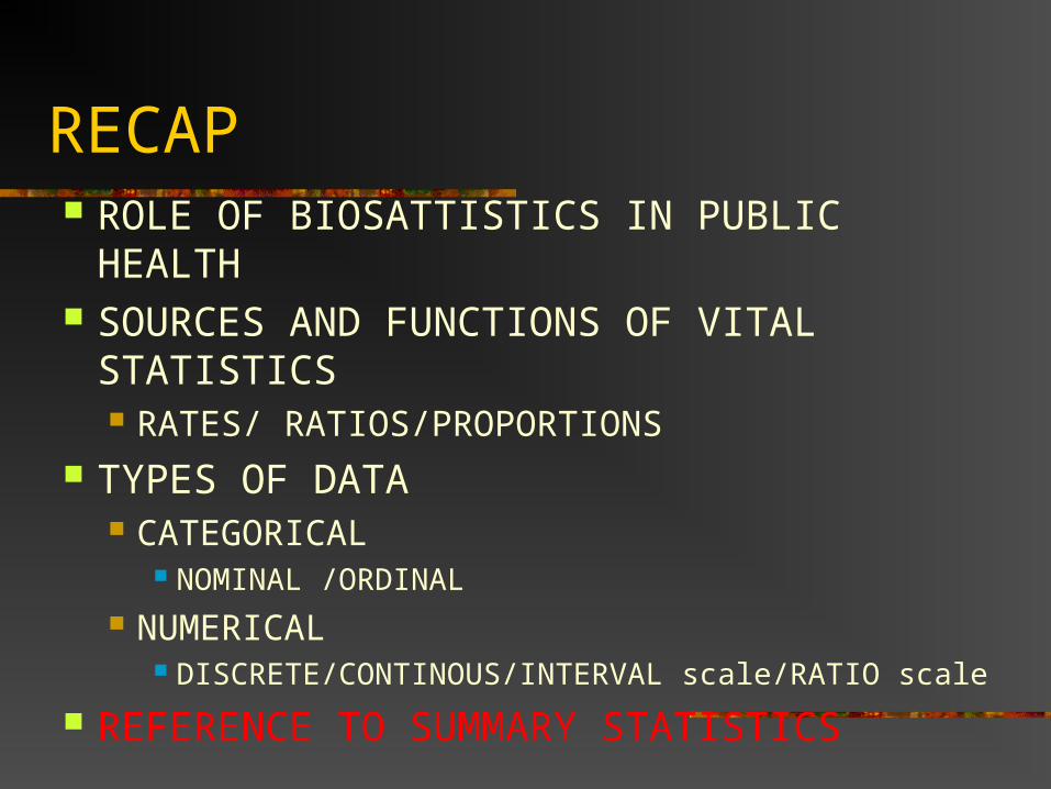
RECAP ROLE OF BIOSATTISTICS IN PUBLIC

HEALTH SOURCES AND FUNCTIONS OF VITAL

STATISTICS RATES/ RATIOS/PROPORTIONS

TYPES OF DATA CATEGORICAL

NOMINAL /ORDINAL NUMERICAL

DISCRETE/CONTINOUS/INTERVAL scale/RATIO scale

REFERENCE TO SUMMARY STATISTICS

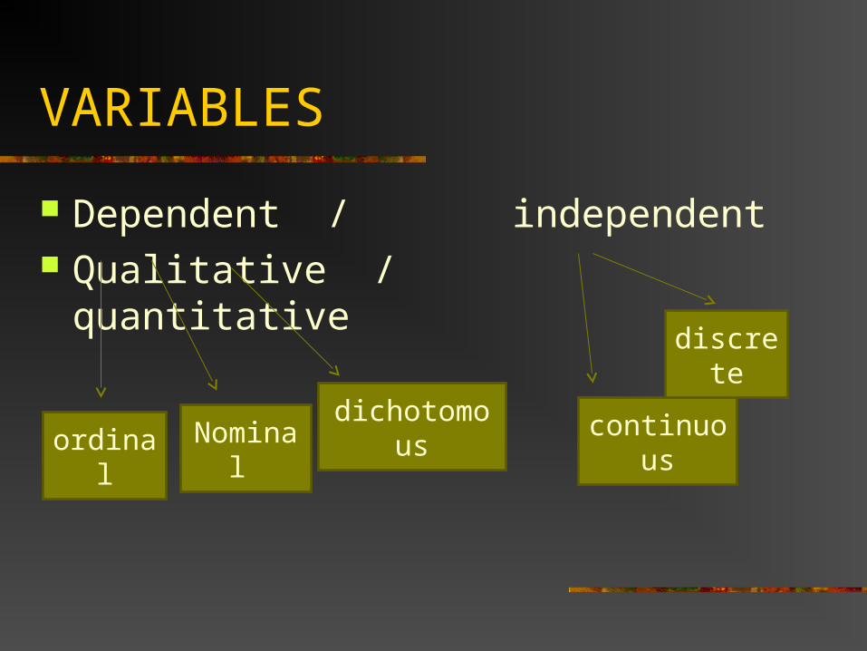
VARIABLES

Dependent / independent Qualitative / quantitative

ordinal Nominal dichotomous continuous

discrete

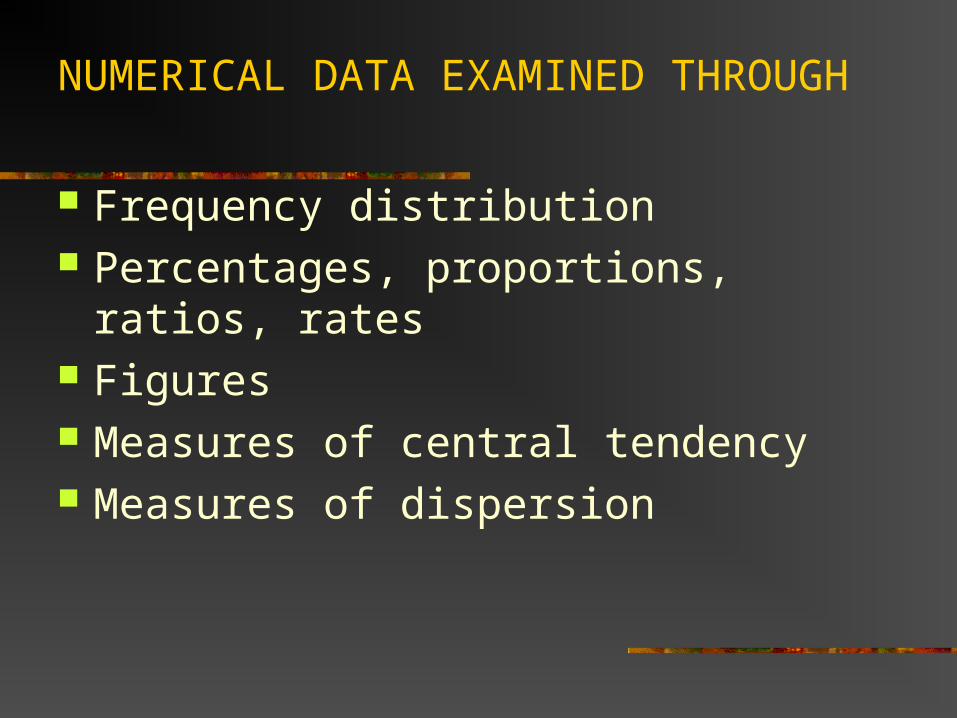
NUMERICAL DATA EXAMINED THROUGH

Frequency distribution Percentages, proportions, ratios, rates Figures Measures of central tendency Measures of dispersion

LEARNING OBJECTIVES

From frequency tables to distributions

Types of Distributions: Normal, Skewed

Central Tendency: Mode, Median, Mean

Dispersion: Variance, Standard Deviation

Descriptive statistics are concerned with describing the characteristics of

frequency distributions

Where is the center? What is the range? What is the shape [of the

distribution?

Frequency Distributions

Simple depiction of all the data Graphic — easy to understand Problems

Not always precisely measured Not summarized in one number or datum

Frequency TableTest Scores

Observation Frequency

65 1

70 2

75 3

80 4

85 3

90 2

95 1

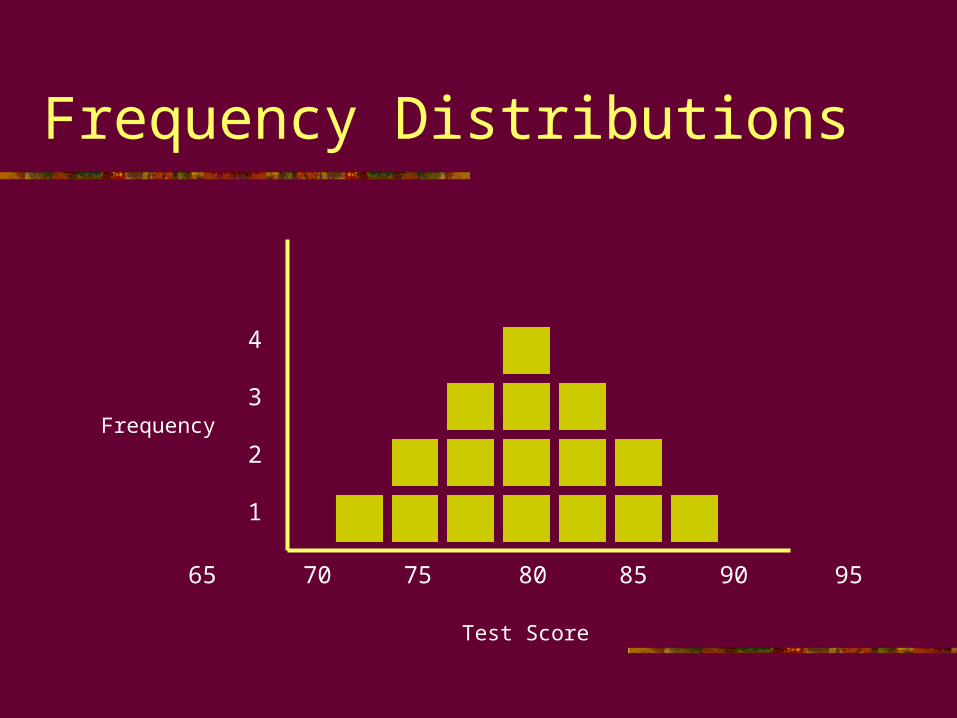
Frequency Distributions

Test Score

Frequency

4

3

2

1

65 70 75 80 85 90 95

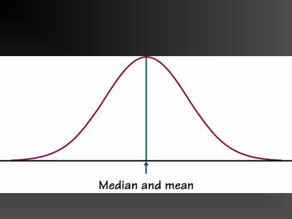
Normally Distributed Curve

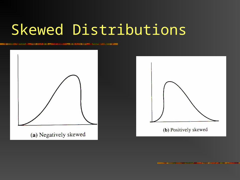
Skewed Distributions

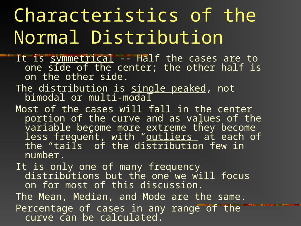
Characteristics of the Normal DistributionIt is symmetrical -- Half the cases are to one side of

the center; the other half is on the other side.The distribution is single peaked, not bimodal or

multi-modalMost of the cases will fall in the center portion of the

curve and as values of the variable become more extreme they become less frequent, with “outliers” at each of the “tails” of the distribution few in number.

It is only one of many frequency distributions but the one we will focus on for most of this discussion.

The Mean, Median, and Mode are the same.Percentage of cases in any range of the curve can be

calculated.

Summarizing Distributions

Two key characteristics of a frequency distribution are especially important when summarizing data or when making a prediction from one set of results to another:

Central Tendency What is in the “Middle”? What is most common? What would we use to predict?

Dispersion How Spread out is the distribution? What Shape is it?

Measures of Central Tendency

The goal of measures of central tendency is to come up with the one single number that best describes a distribution of scores.

Lets us know if the distribution of scores tends to be composed of high scores or low scores.

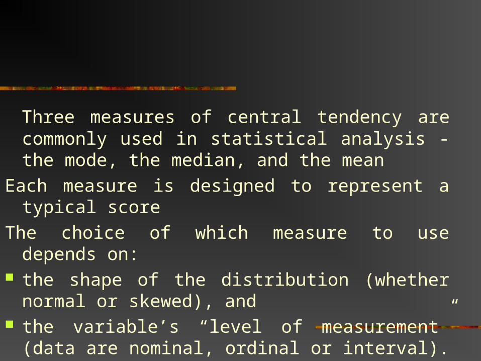
Three measures of central tendency are commonly used in statistical analysis - the mode, the median, and the mean

Each measure is designed to represent a typical score

The choice of which measure to use depends on: the shape of the distribution (whether normal or

skewed), and the variable’s “level of measurement” (data are

nominal, ordinal or interval).

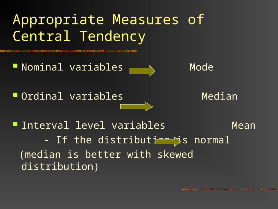
Appropriate Measures of Central Tendency

Nominal variables Mode

Ordinal variables Median

Interval level variables Mean

- If the distribution is normal

(median is better with skewed distribution)

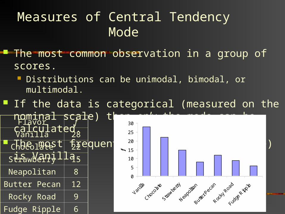
Measures of Central TendencyMode

The most common observation in a group of scores. Distributions can be unimodal, bimodal, or multimodal.

If the data is categorical (measured on the nominal scale) then only the mode can be calculated.

The most frequently occurring score (mode) is Vanilla.

0

5

10

15

20

25

30

Vanilla

Choco

late

Strawbe

rry

Neapo

litan

Butte

r Pec

an

Rocky

Roa

d

Fudg

e Ripp

le

fFlavor f

Vanilla 28

Chocolate 22

Strawberry 15

Neapolitan 8

Butter Pecan 12

Rocky Road 9

Fudge Ripple 6

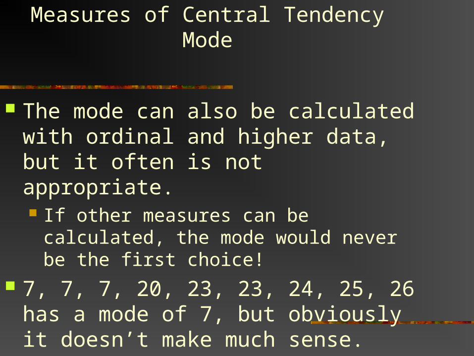
Measures of Central TendencyMode

The mode can also be calculated with ordinal and higher data, but it often is not appropriate. If other measures can be calculated, the

mode would never be the first choice! 7, 7, 7, 20, 23, 23, 24, 25, 26 has a mode

of 7, but obviously it doesn’t make much sense.

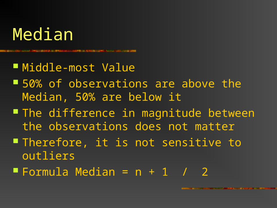
Median

Middle-most Value 50% of observations are above the

Median, 50% are below it The difference in magnitude between the

observations does not matter Therefore, it is not sensitive to outliers Formula Median = n + 1 / 2

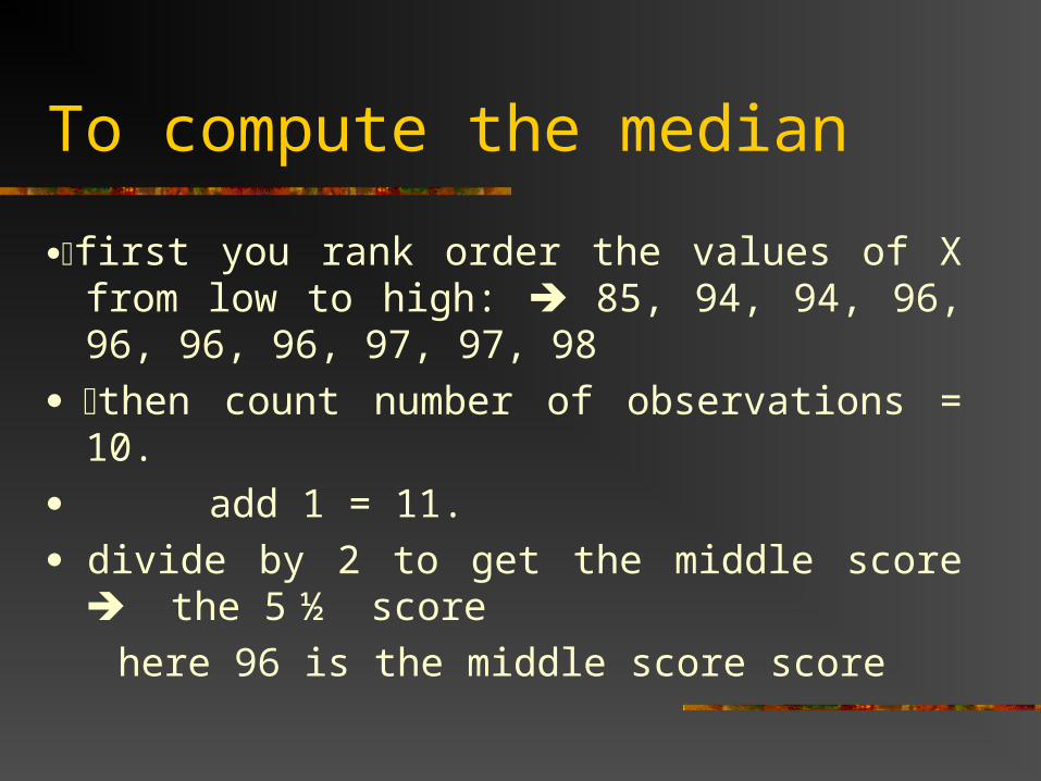
To compute the median

first you rank order the values of X from low to high: 85, 94, 94, 96, 96, 96, 96, 97, 97, 98

then count number of observations = 10.

add 1 = 11.

 divide by 2 to get the middle score the 5 ½ score

here 96 is the middle score score

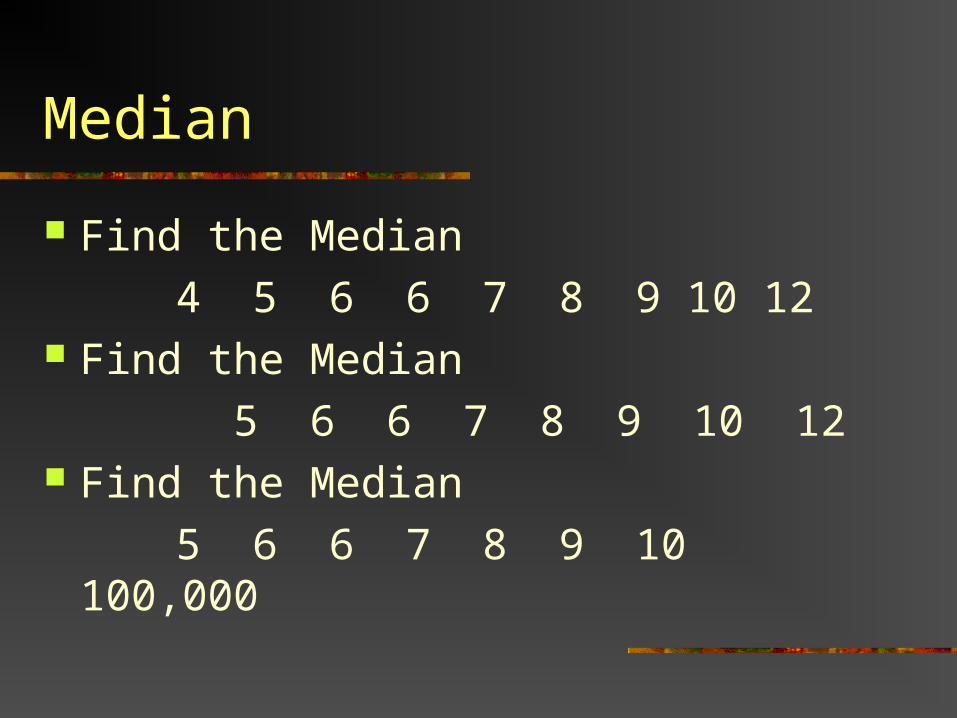
Median

Find the Median

4 5 6 6 7 8 9 10 12 Find the Median

5 6 6 7 8 9 10 12 Find the Median

5 6 6 7 8 9 10 100,000

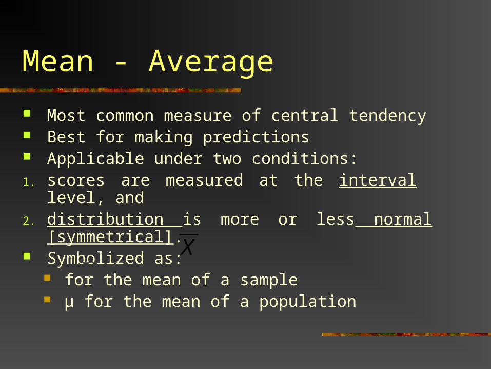
Mean - Average

Most common measure of central tendency Best for making predictions Applicable under two conditions:1. scores are measured at the interval level, and2. distribution is more or less normal [symmetrical]. Symbolized as:

for the mean of a sample μ for the mean of a population

X

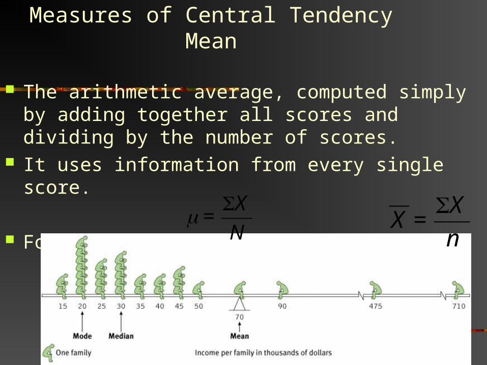
Measures of Central TendencyMean

The arithmetic average, computed simply by adding together all scores and dividing by the number of scores.

It uses information from every single score.

For a population: For a Sample:N

X=

n

X=X

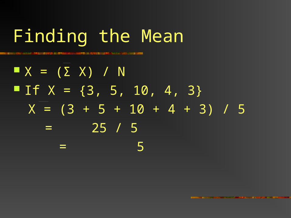
Finding the Mean

X = (Σ X) / N If X = {3, 5, 10, 4, 3}

X = (3 + 5 + 10 + 4 + 3) / 5

= 25 / 5

= 5

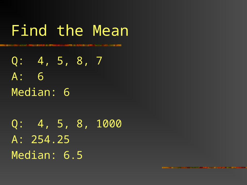
Find the Mean

Q: 4, 5, 8, 7

A: 6

Median: 6

Q: 4, 5, 8, 1000

A: 254.25

Median: 6.5

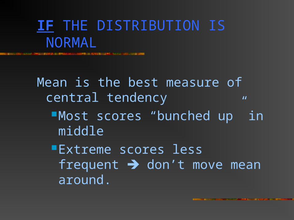
IF THE DISTRIBUTION IS NORMAL

Mean is the best measure of central tendencyMost scores “bunched up” in middleExtreme scores less frequent

don’t move mean around.

Measures of Central Tendency ;Mean

If data are perfectly normal, then the mean, median and mode are exactly the same.

I would prefer to use the mean whenever possible since it uses information from EVERY score.

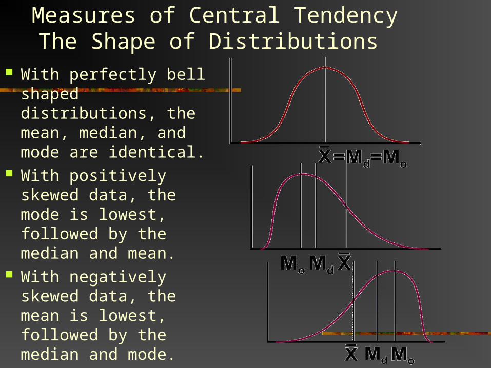
Measures of Central TendencyThe Shape of Distributions

With perfectly bell shaped distributions, the mean, median, and mode are identical.

With positively skewed data, the mode is lowest, followed by the median and mean.

With negatively skewed data, the mean is lowest, followed by the median and mode.

Measures of Central TendencyUsing the Mean to Interpret DataDescribing the Population Mean

Remember, we usually want to know population parameters, but populations are too large.

So, we use the sample mean to estimate the population mean.

X

How well does the mean represent the scores in a distribution? The logic here is to determine how much spread is in the scores. How much do the scores "deviate" from the mean? Think of the mean as the true score or as your best guess. If every X were very close to the Mean, the mean would be a very good predictor.

If the distribution is very sharply peaked then the mean is a good measure of central tendency and if you were to use the mean to make predictions you would be right or close much of the time.

Why can’t the mean tell us everything?

Mean describes Central Tendency, what the average outcome is.

We also want to know something about how accurate the mean is when making predictions.

The question becomes how good a representation of the distribution is the mean? How good is the mean as a description of central tendency -- or how good is the mean as a predictor?

Answer -- it depends on the shape of the distribution. Is the distribution normal or skewed?

What if scores are widely distributed?

The mean is still your best measure and your best predictor, but your predictive power would be less.

How do we describe this? Measures of variability

Mean Deviation Variance Standard Deviation

Measures of Variability

Central Tendency doesn’t tell us everything

Dispersion/Deviation/Spread tells us a lot about how a variable is distributed.

We are most interested in Standard Deviations (σ) and Variance (σ2)

DispersionOnce you determine that the variable of interest is

normally distributed, ideally by producing a

histogram of the scores, the next question to be

asked about the NDC is its dispersion: how spread out are the scores around the mean.

Dispersion is a key concept in statistical thinking.

The basic question being asked is how much do the scores deviate around the Mean? The more “bunched up” around the mean the better your ability to make accurate predictions.

Mean Deviation

The key concept for describing normal distributions

and making predictions from them is called

deviation from the mean.

We could just calculate the average distance between each observation and the mean.

We must take the absolute value of the distance, otherwise they would just cancel out to zero!

Formula:

| |iX X

n

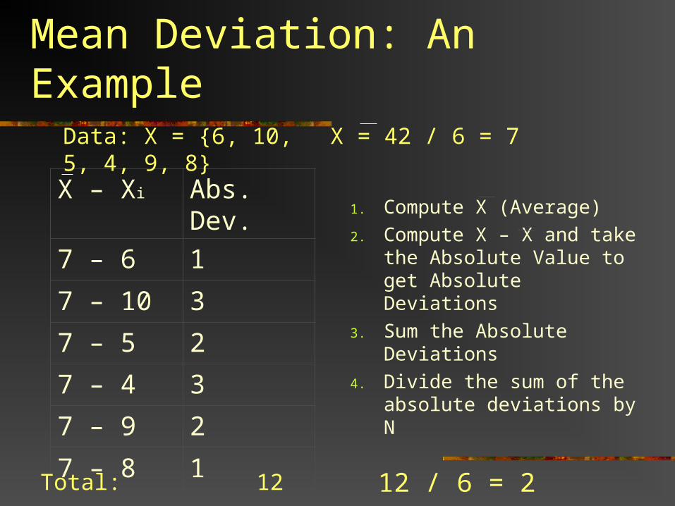
Mean Deviation: An Example

1. Compute X (Average)

2. Compute X – X and take the Absolute Value to get Absolute Deviations

3. Sum the Absolute Deviations

4. Divide the sum of the absolute deviations by N

X – Xi Abs. Dev.

7 – 6 1

7 – 10 3

7 – 5 2

7 – 4 3

7 – 9 2

7 – 8 1

Data: X = {6, 10, 5, 4, 9, 8} X = 42 / 6 = 7

Total: 12 12 / 6 = 2

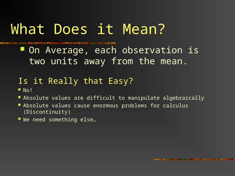
What Does it Mean? On Average, each observation is two units

away from the mean.

Is it Really that Easy? No! Absolute values are difficult to manipulate algebraically Absolute values cause enormous problems for calculus (Discontinuity) We need something else…

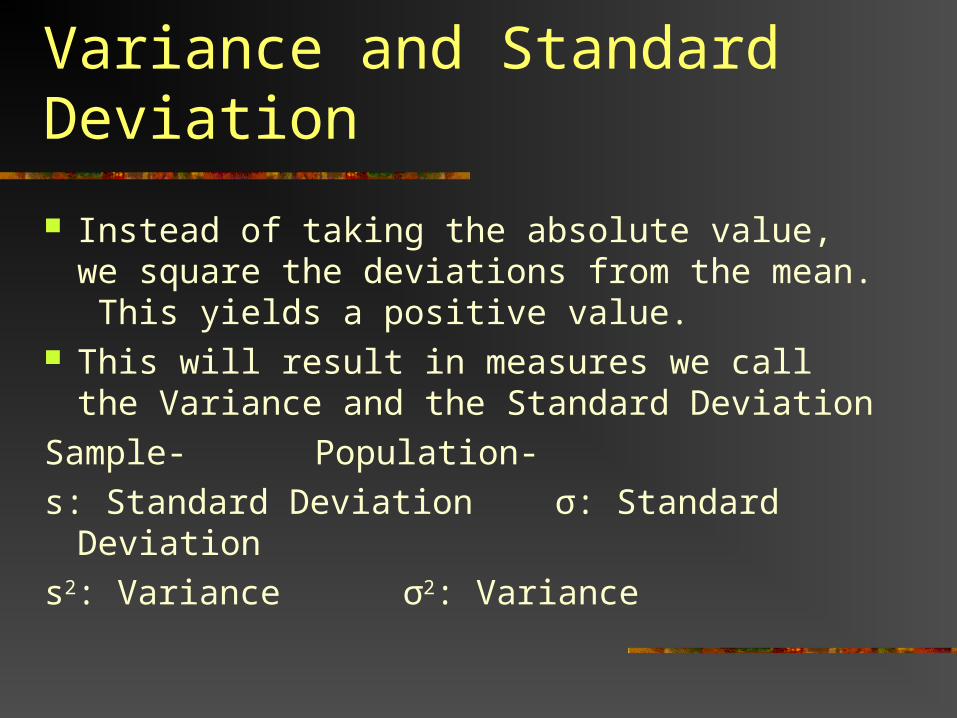
Variance and Standard Deviation

Instead of taking the absolute value, we square the deviations from the mean. This yields a positive value.

This will result in measures we call the Variance and the Standard Deviation

Sample- Population-

s: Standard Deviation σ: Standard Deviation

s2: Variance σ2: Variance

Calculating the Variance and/or Standard Deviation

Formulae:

Variance:

Examples Follow . . .

2( )iX Xs

N

2

2 ( )iX Xs

N

Standard Deviation:

Example:

-1 1

3 9

-2 4

-3 9

2 4

1 1

Data: X = {6, 10, 5, 4, 9, 8}; N = 6

Total: 42 Total: 28

Standard Deviation:

76

42

N

XX

Mean:

Variance:2

2 ( ) 284.67

6

X Xs

N

16.267.42 ss

XX 2)( XX X

6

10

5

4

9

8

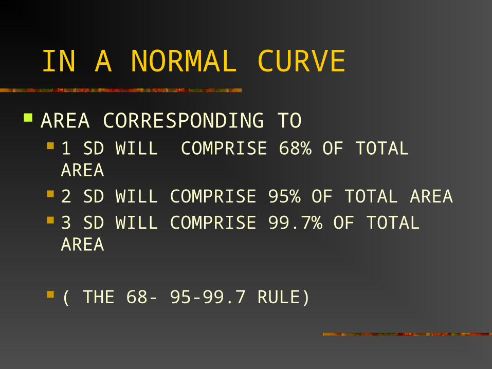
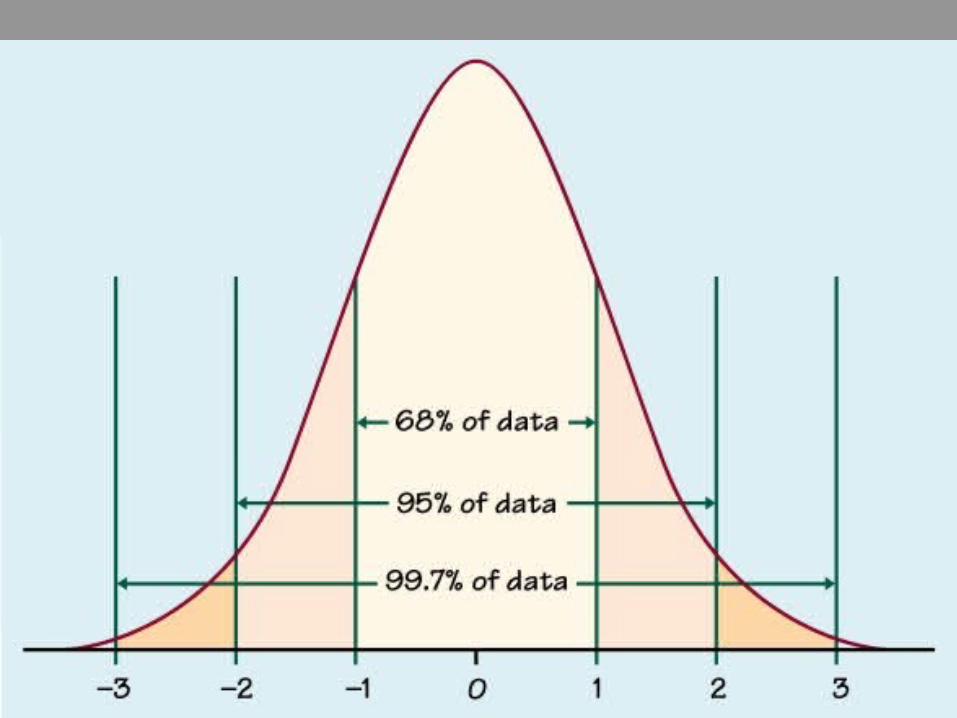
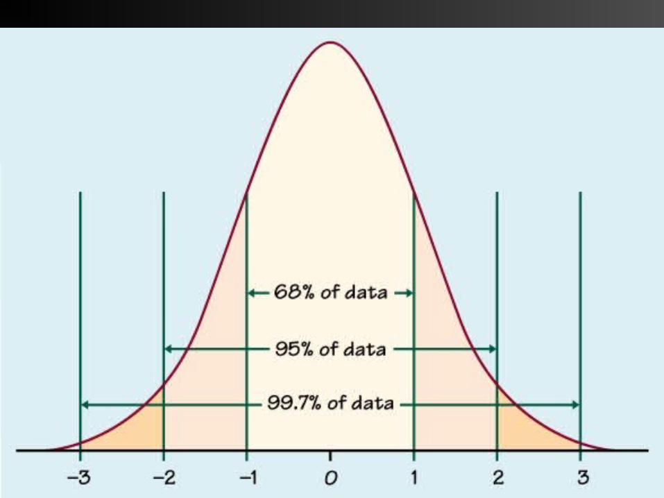
IN A NORMAL CURVE

AREA CORRESPONDING TO 1 SD WILL COMPRISE 68% OF TOTAL AREA 2 SD WILL COMPRISE 95% OF TOTAL AREA 3 SD WILL COMPRISE 99.7% OF TOTAL

AREA

( THE 68- 95-99.7 RULE)

COEFFICIENT OF VARIANCE

Measures the spread the spread of data set as a proportion of its mean

Expressed as percentage It is ratio of sample standard deviation to

sample mean. CV of population is based on expected value and SD of a random variable

CV = standard deviation/mean x 100

PERCENTILES

Give variability of the distribution The p’th percentile of distribution is the

value such that p% of observations fall at or below it

Median is the 50th percentile Used in calculation of growth charts for

nutritional surveillance and monitoring

QUARTILES

Values that divide the data into four groups containing equal numbers of observations

Quartiles are the 25th and 75th percentiles First quartile is the median of observations

below the median of the complete data set, Third quartile is the median of observations

above the median of the complete data.

RANGE

The range of a sample /data set is the difference between the largest and smallest observed value of some quantifiable characteristic.

A simple summary measure but crude Like mean it is affected by extreme values Data: 2,3,4,5,6,6,6,7,7,8,9 RANGE 2- 9= 7

INTERQUARTILE RANGE(IQR)

Calculated by taking difference between upper and lower quartiles

IQR is the width of an interval which contains middle 50% of sample

Smaller than range and less affected by outliers.

Data: 2,3,4,56,6,6,7,7,8,9 Upper quartile=7, lower quartile=4, IQR=3

QUESTIONS ARE WELCOME

FEELING READY FOR RESEARCH AND APPROPRIATE DATA

COLLECTION ????????

THERE WILL BE A CLASS TEST OF 50 MCQs OUT OF SUBJECTS STUDIED SO FAR ON

15 TH OCT 2012