sample size determination for categorical responsescgga/jfs2009mavridis.pdf · sample size...

Dimitris Mavridis,1 Ph.D. and Colin G.G. Aitken,1 Ph.D.

Sample Size Determination forCategorical Responses

ABSTRACT: Procedures are reviewed and recommendations made for the choice of the size of a sample to estimate the characteristics (some-times known as parameters) of a population consisting of discrete items which may belong to one and only one of a number of categories withexamples drawn from forensic science. Four sampling procedures are described for binary responses, where the number of possible categories is onlytwo, e.g., licit or illicit pills. One is based on priors informed from historical data. The other three are sequential. The first of these is a sequentialprobability ratio test with a stopping rule derived by controlling the probabilities of type 1 and type 2 errors. The second is a sequential variation ofa procedure based on the predictive distribution of the data yet to be inspected and the distribution of the data that have been inspected, with a stop-ping rule determined by a prespecified threshold on the probability of a wrong decision. The third is a two-sided sequential criterion which stopssampling when one of two competitive hypotheses has a probability of being accepted which is larger than another prespecified threshold. The fifthprocedure extends the ideas developed for binary responses to multinomial responses where the number of possible categories (e.g., types of drug ortypes of glass) may be more than two. The procedure is sequential and recommends stopping when the joint probability interval or ellipsoid for theestimates of the proportions is less than a given threshold in size. For trinomial data this last procedure is illustrated with a ternary diagram with anellipse formed around the sample proportions. There is a straightforward generalization of this approach to multinomial populations with more thanthree categories. A conclusion provides recommendations for sampling procedures in various contexts.

KEYWORDS: forensic science, sample size, evidence evaluation, likelihood ratio, ternary diagram, multinomial data, misleading evidence,power priors

Sample size determination (SSD) is a crucial aspect of anyexperimental design and there have been a number of papersaddressing this subject both from a frequentist and a Bayesianapproach. A review of the subject up to the mid-1990’s can befound in Ref. (1) and references therein. Most examples in the liter-ature come from medical studies and from the quality assessmentof products. Another field where SSD may play a crucial role inthe saving of resources is in forensic analysis. For instance, theremay be a consignment of discrete units with certain proportionscontaining illegal materials of different types. Such units may bepills (which may be drugs, possibly of more than one type), CDsor pornographic computer files. The traditional approach to SSDfrom a frequentist perspective is to control some aspects of thesampling distributions of the statistics that are used for drawinginference and to define null and alternative hypotheses for the valueof the characteristic of interest (e.g., proportion of pills of a certaintype). The sample size is then determined by controlling the proba-bilities of type 1 and type 2 errors, respectively, the probabilities ofrejecting the null hypothesis (e.g., that the proportion of pills is lessthan a certain value) when it is true and of not rejecting the nullhypothesis when it is false.

Emphasis is given here on the use of Bayesian methodology inwhich inferences are made directly about the characteristic of inter-est which is categorical. The characteristic, conventionally denotedh, is considered to be random and to have an associated probabilitydistribution in some relevant population from which all relevantinformation about h may be obtained. Such information can includethe mean, the variance and distributional results such that the prob-ability that h is greater than a certain value, for example, may be

determined. An extension to consider quantities is described inRefs (2,3).

It is common in forensic analysis to encounter a consignment ofdiscrete units, some of which may contain illegal material. Exam-ples of such units are pills, some of which may be illicit, CDs,some of which may be pirated, or computer files, some of whichmay be pornographic. For illicit drugs in pills there may be two ormore mutually exclusive categories for classification (e.g., powdercocaine, crack cocaine, heroin, LSD, and marijuana). Consider asample of known size, n say, taken from the consignment. Whenthere are only two mutually exclusive categories, such as licit andillicit, a common distribution associated with the number of pills inone of the categories, conditional on the total number of pills inthe sample, is the binomial distribution. When there are more thantwo mutually exclusive categories, the analogous distribution forthe number of pills in each of the categories is known as a multino-mial distribution. Izenman points out that inaccuracies may occurwhen the whole seizure is being analyzed due to time and man-power constraints (4). Furthermore, he argues that certain chemicaltesting destroys the evidence and that evidence may need tobe shown to the jury or given to the defense to make their owntesting. Also forensic scientists may be exposed to potential healthhazards through airborne dust or physical contact. Thus, for variousreasons, as little analysis as possible is desirable so a sample is ana-lyzed rather than every member of the consignment. Criteria arerequired in order to give meaning to the phrase ‘‘as little...aspossible.’’

Many simple approaches to the determination of a sample sizehave been adopted. These approaches include choosing the samplesize to be the size of the square root of the size of the whole con-signment. Other rules are to analyze a number equal to half thesquare root of the size of the whole consignment, or equal to acertain proportion, such as 10%, of the size of the whole consign-ment. These methods, although simple to remember, have little or

1School of Mathematics and The Joseph Bell Centre for Forensic Statis-tics and Legal Reasoning, The King’s Buildings, The University of Edin-burgh, Mayfield Road, Edinburgh EH9 3JZ, U.K.

Received 24 Mar. 2007; and in revised form 31 May 2008; accepted 8Aug. 2008.

J Forensic Sci, January 2009, Vol. 54, No. 1doi: 10.1111/j.1556-4029.2008.00920.x

Available online at: www.blackwell-synergy.com

� 2008 American Academy of Forensic Sciences 135

no statistical justification and may lead to the inspection of quanti-ties of pills considerably in excess of those required for an infer-ence to be made that is sufficient for legal purposes. Methodsbased on the beta and binomial distributions for samples in whichall sampled items are illicit are described in Ref. (5) and extendedhere to sequential sampling. Samples contain items of more thanone category. For binary models these categories could be licit andillicit in drug cases and four models are described in this context.

A fifth model is described for samples with more than two catego-ries. The method described here assumes that the number of catego-ries is known. The purpose of the sampling is to estimate theproportions of each category in the consignment. Further work isrequired in order to develop a sampling protocol for situations inwhich the number of categories is unknown. The example describedhere considers three categories for pills in a drug case where the cate-gories are licit, ecstasy, and LSD. Other examples include:

• a mixture of glass fragments of a known number of categories;• an autosomal locus with a known number of different alleles;• soil which is a mixture of several different soil types;• a pollen composition which is a mixture of several different

types.

In each example, the purpose of the sampling is to estimate theproportion of each type or category.

Binomial Sampling

Consider circumstances in which a sample of size n items aretaken at random and without replacement from a large populationof size m. Items may be assigned to one and only one of two cate-gories, conventionally known as ‘‘success’’ and ‘‘failure.’’ As men-tioned above, examples include illicit or licit drugs, pirated or legalCDs, pornographic or nonpornographic computer files.

Consider the case of illicit or licit drugs. In some jurisdictions,the numbers of pills seized is a contributory factor in the determi-nation of the defendant’s sentence and hence accurate estimation ofthese numbers, with knowledge of the associated uncertainty in theestimation, is important. These numbers may be obtained from esti-mates of the proportions of drugs in each category by multiplica-tion of these estimated proportions by the consignment size. Theprocedures described here consider estimation of proportions as thisis statistically the best way to proceed. It is straightforward to trans-form the results into numbers in a consignment.

Denote the proportion of items in the population that are catego-rized as successes (or, more briefly, known as ‘‘successes’’) as h. Inthe context of illicit and licit drugs, the proportion of pills that areillicit is of interest so a ‘‘success’’ would be an illicit tablet. Thisinformation about the population is then translated to record that foran item drawn at random from the population (pill from the con-signment), the probability it is a success (illicit) is h. The populationis deemed to be sufficiently large relative to the sample size thatthe probabilities for successive drawings without replacement fromthe sample to be successes may be treated as constant and equal toh; i.e., sampling is taken to be equivalent to sampling with replace-ment. For small consignments, analyses using the beta–binomialdistribution are appropriate and described in the section on ‘‘Predic-tive sample size determination.’’ Let X denote the phrase ‘‘the num-ber of drawings from a sample of size n that are successes’’ (thenumber of pills in the sample that are illicit) and let x be the sym-bol denoting the number of successes (illicit pills) in a sample ofsize n. Thus, the phrase ‘‘the probability the number of drawingsfrom a sample of size n that are successes equals x’’ may be writtensymbolically as Pr(X ¼ x). When there are two, and only two

categories for a population into which an item may be placed,with probabilities h and (1 ) h), respectively, then the number ofsuccesses, X, in a sample of size n, has a binomial distribution

PrðX ¼ xjn; hÞ ¼ n

x

� �hxð1� hÞðn�xÞ; 0 < h < 1; x ¼ 0; 1; . . . ; n

The vertical bar | denotes conditioning in that symbols to theright of the bar are taken to be known. Here these are n, thesample size and h, the probability of a success. The expressionto the left of the bar is taken to be unknown and the expressionwhose probability it is desired to determine. Thus, the probabil-ity statement concerns the probability the number of successesequals x, conditional on (or ‘‘given’’) n, the sample size and h,the probability of a success. Sometimes, as in the discussion ofpower priors, this function is expressed as a function of h and itis then known as a likelihood

Lðhjn;X ¼ xÞ ¼ n

x

� �hxð1� hÞðn�xÞ; 0 < h < 1; x ¼ 0; 1; . . . ; n

ð1Þ

The sample proportion h ¼ x=n provides a good estimate of h.

The variance of h including a so-called ‘‘finite population correc-tion’’ (m ) n) ⁄ (m ) 1) is

hð1� hÞn

m� n

m� 1

� �(6). As an example of the use of the finite population correctionconsider the example where the sample is the whole populationso that n ¼ m. Then the sample proportion is the populationproportion and there is no uncertainty; the variance is zerowhich is the result given from the expression of the varianceusing the finite population correction. If the sampling fractionn ⁄ m is low the finite population correction (m ) n) ⁄ (m ) 1) ¼1 ) (n ) 1) ⁄ (m ) 1) can be ignored. Assume that the sampleproportion is asymptotically Normally distributed. Then

h � N h;hð1� hÞ

n

� �ð2Þ

One criterion for the choice of sample size in such a contextis that there should be 100(1 ) a)% confidence that the sampleproportion lies within an interval of desired length 2d of the trueproportion h. Then

za=2

ffiffiffiffiffiffiffiffiffiffiffiffiffiffiffiffiffiffiffihð1 � hÞ

n

r� d

and hence n � z2a=2hð1 � hÞ=d2 where za/2 is the 100(1 ) a/2)%

point of the standard Normal distribution. For example, whena ¼ 0.05, za/2 ¼ 1.96, the 97.5% point of the standard Normaldistribution. As h is not known in advance there are two coursesof action. One is to use a prior subjective estimate for h. The otheris to use the value of h for which h(1 ) h) is a maximum which iswhen h ¼ 0.5. This latter choice leads to the rule

n �z2a=2

4d2ð3Þ

which is conservative in that it gives the largest sample sizenecessary to satisfy the criterion.

Thus, for a ¼ 0.05 and d ¼ 0.01, the sample size n shouldbe greater than or equal to 1.962 ⁄ (4 · 0.0001) ¼ 3.84 ⁄0.0004 ¼

136 JOURNAL OF FORENSIC SCIENCES

9600; i.e., to obtain an estimate of the true proportion in a categoryto within 0.01 of the true proportion, with 95% confidence, a sam-ple of size 9600 items is needed. This is a large sample but also astringent criterion. To obtain an estimate of the true proportion in acategory to within 0.1 of the true proportion, with 95% confidence,a sample of size 96 items is needed. The sample size has to beincreased by a factor of 100 to narrow the width of the interval bya factor of 10. As an example, for consignments of CDs, with 95%confidence, an estimate could be given to within 0.1 of the trueproportion of pirated CDs in a consignment if 96 were examined.In practice, it is suggested 100 CDs be examined.

In a Bayesian paradigm, uncertainty in parameter estimation ismodeled with probability distributions for the parameters of interest.The beta distribution is commonly chosen to represent uncertaintyabout the parameter h and details are given in the Appendix. Thisdistribution is a so-called conjugate prior distribution for the bino-mial distribution in that the posterior distribution is also a beta dis-tribution, but with different parameters.

Let uncertainty about h, the probability of success for an itemdrawn in a sample of size n from a population, be represented witha beta distribution beta(m1,m2). The number of successes, X, in thesample has a binomial distribution. The combination of the betaprior and binomial distribution gives a posterior distributionbeta(m1 + x, n ) x + m2) for h which is also a beta distribution, asa result of the property of conjugacy. The probability densityfunction is

f ðhjm1 þ x; m2 þ n� xÞ

¼ Cðnþ m1 þ m2ÞCðm1 þ xÞCðm2 þ n� xÞ h

m1þx�1ð1� hÞn�xþm2�1;

m1 > 0; m2 > 0; 0 < h < 1; x ¼ 0; 1; . . . ; n ð4Þ

The Bayesian approach provides answers to the questions ofinterest of the forensic scientist in that it provides probabilitiesfor the uncertainties about the probabilities of success (propor-tions of illicit drugs, proportions of pirated CDs, or porno-graphic files).

This is in contrast to the frequentist approach in which confi-dence limits are provided. Confidence limits are limits which applyin the long run in that if identical conditions apply many times thenthese limits will contain the true answer a certain proportion of thetime; no statement is made about the particular occasion underinspection. Thus, as stated above, for consignments of CDs, the95% confidence limits are such that in 95% of cases in which CDsare examined, the proportion of pirated CDs in a sample of size 96will be within 0.1 of the true proportion of pirated CDs in thewhole consignment.

Likelihood Principle

A method that has been widely used for evaluating statisticalevidence for one hypothesis versus another is the likelihood ratio.The term ‘‘likelihood ratio’’ is used because reference is made to‘‘how likely the data x are if one hypothesis (denoted H2 say) is truerelative to how likely the data are if another hypothesis (denoted H1

say) is true.’’ Hacking (7) defined the likelihood law as

If one hypothesis, H1, implies that a random variable X takes thevalue x with probability f(x|H1), while another hypothesis, H2,implies that the probability is f(x|H2), then the observation X ¼ xis evidence supporting H2 over H1 if f(x|H2) > f(x|H1), and thelikelihood ratio, LR,

f ðxjH2Þf ðxjH1Þ

measures the strength of that evidence.This definition provides a common approach to the evaluation of

evidence in forensic science when H2 is taken as the prosecutionproposition, H1 as the defense proposition, and x as the evidencethat is being evaluated (8). Note that in evidence evaluation theterm proposition is preferred to the term hypothesis, because of thestatistical frequentist connotations of the latter term. The term‘‘proposition’’ will be used from now on as far as is appropriate.

The LR may also be given as the ratio of the posterior odds infavor of H2 to the prior odds in favor of H2:

LR ¼ f ðxjH2Þf ðxjH1Þ

¼ f ðH2jxÞ=f ðH1jxÞf ðH2Þ=f ðH1Þ

ð5Þ

where f(H1) and f(H2) are the prior probabilities, the probabili-ties that H1 and H2 are true, respectively, prior to the conductof the experiment, their ratio is the prior odds in favor of H2,f(H1|x) and f(H2|x) are the posterior probabilities for proposi-tions H1 and H2, and their ratio is the posterior odds in favor ofH2. The expression f(H2|x), for example, may be read as theprobability H2 is true, given x successes out of a sample of sizen. The LR is the factor which converts prior odds into posteriorodds. An interpretation of the likelihood ratio is to say that theevidence is so many times more likely if H2 is true than if H1

is true.The LR is non-negative and can take values greater than 1. An

LR equal to one indicates that the evidence is equally probableunder either of the two competing propositions. Values of LRgreater than one indicate that the evidence supports H2 over H1

and values smaller than one favor H1 over H2. For ease of interpre-tation and for the better understanding of the strength of the evi-dence, the possible values of the LR can be divided into regions toindicate the differing strengths of the evidence. Therefore, it maybe taken that LRs close to one represent weak evidence and thatLRs greater than some threshold t (t > 1) or less than t)1 representmoderate or strong evidence in favor of H2 or H1, respectively,according to some numerical criterion for t. Thresholds (t ¼ 8and t ¼ 32) with conventional descriptions ‘‘weak,’’ ‘‘moderate,’’and ‘‘strong’’ have been suggested by Royall (9) such that

• weak evidence– for H2 over H1: 1 £ LR < 8,– for H1 over H2: 1/8 < LR £ 1;

• moderate evidence– for H2 over H1: 8 £ LR < 32,– for H1 over H2: 1/32 < LR £ 1/8;

• strong evidence– for H2 over H1: LR ‡ 32,– for H1 over H2: LR £ 1/32.

There is a nonzero probability that the likelihood ratio may yieldstrong evidence supporting H2 over H1 when, in fact, H1 is correct,or vice versa. The wrong proposition is then accepted. In such acase the evidence is known as misleading evidence. A probabilisticlimit on this situation is described.

Probability of Accepting the Wrong Proposition

Consider two propositions of interest H1 and H2 concerning abinomial characteristic, h say, such that H1:h £ hl and H2:h ‡ hu.This characteristic could be the proportion of illicit drugs in a

MAVRIDIS AND AITKEN • SAMPLE SIZE DETERMINATION 137

consignment (and by multiplication, the total number in the con-signment) with interest being in the value for sentencing purposes.A binomial experiment (i.e., one with a fixed number of items withtwo possible categories into which items can be assigned, with aconstant assignation probability for each trial and such that eachtrial is independent of all other trials) is conducted and x successesare observed out of n trials. The LR is given by f(x|H2) ⁄ f(x|H1)where f is the probability function of the binomial distribution. Theprobability of H2 being accepted is

f ðH2jxÞ ¼f ðxjH2Þf ðH2Þ

f ðxjH1Þf ðH1Þ þ f ðxjH2Þf ðH2Þð6Þ

which can be rewritten as

f ðH2jxÞ ¼LRf ðH2Þ

f ðH1Þ þ LRf ðH2Þð7Þ

by dividing the numerator and denominator of the right-handside by f(x|H1). By further dividing both the numerator anddenominator of the right-hand side by f(H1),

f ðH2jxÞ ¼LR f ðH2Þ

f ðH1Þ

1þ LR f ðH2Þf ðH1Þ

ð8Þ

There are two and only two propositions. If H2 is not true thenH1 is true. Thus, f(H2|x) + f(H1|x) ¼ 1 and hence

f ðH1jxÞ ¼1

1þ LR f ðH2Þf ðH1Þ

ð9Þ

It is evident from Eqs (8) and (9) that the probability of the truthof either of the two propositions given the data (x successes out ofn items sampled) is a function of the likelihood ratio and the priorodds f(H2) ⁄ f(H1) in favor of H2.

If both competing propositions are equiprobable a priorif ðH1Þ ¼ f ðH2Þ ¼ 1

2

� �, then

f ðH2jxÞ ¼LR

LRþ 1

and

f ðH1jxÞ ¼1

LRþ 1

It can be deduced that for any given constant k > 0, Pr(LR ‡k|H1 is true) £ 1 ⁄k; i.e., the probability of evidence that supportsH2 with an LR ‡ k when H1 is true is £ 1 ⁄k. Evidence that sup-ports H2 when H1 is true is misleading. Consider S to be the set ofvalues of x that produce a value of the LR in favor of H2 versusH1 of at least k. For x 2 S, f(x|H2) ⁄ f(x|H1) ‡ k and hencef(x|H1) £ f(x|H2) ⁄k, where 2 is read as ‘‘is a member of.’’ ThenPr(S) ¼

Px 2 S f(x|H1) £

Px 2 S f(x|H2) ⁄k £ 1/k. Equation (7)

enables the formation of a scale of evidence in favor of one propo-sition or the other. For instance, sampling could be stopped whenthe probability that one proposition is correct, given the sampleddata, is above some predefined threshold.

Sequential Sampling

Sequential analysis was developed during the Second WorldWar (10) mainly because war production and development requiredresults as quickly as possible. In sequential sampling a consignment(of pills, for example) is inspected, usually one item at a time (butsometimes in small batches). After inspection of each item (or

small batch) a decision is made as to whether to continue samplingor to terminate the process. Sampling is terminated when the cumu-lative sample contains enough information to make a decisionbased on some prespecified probabilistic criterion. Analysis happensas the data are collected in contrast with sampling plans where sta-tistical analysis is conducted after a sample of a size fixed inadvance has been collected; see Eq. (3) for an example of a samplesize fixed in advance. Sequential sampling is best used when theemphasis is on decision making and there are well-defined proposi-tions about which decisions can be made. The methods used tomake decisions from sequential sampling are called stopping rules.The accumulated data are analyzed at each step to see if one of thestopping rules has been attained and hence sampling may stop,otherwise sampling is continued.

Large values (>1) of the likelihood ratio constitute statistical evi-dence in favor of one proposition whereas small values (<1) aresupportive of the other proposition. The likelihood ratio may becomputed sequentially as data are inspected. In such a case, sam-pling is stopped when enough data have been collected to supportone of the competing propositions in the sense that the LR isgreater than a threshold t, (e.g., t ¼ 32) or smaller than t)1 (e.g.,1 ⁄32). A well-known test that distinguishes between two competingpropositions by using the likelihood ratio and controlling the proba-bilities of type 1 and type 2 errors is the sequential probability ratiotest (SPRT) (10).

Sequential Probability Ratio Test

Suppose that there are two competing propositions H1 and H2

for the value of the parameter h, where h is the proportion of itemsin the population falling into a certain category. For example, H1

could be that h ¼ h1 and H2 could be that h ¼ h2, respectively.As an example consider a seizure of 5000 pills. The exact size

of the seizure is not important for determination of proportionsexcept that it must be sufficiently large that sampling of the pillsmay be considered to be with replacement; i.e., the proportions oflicit and illicit pills remain effectively unchanged with the removalof a few pills from the consignment. The exact size of the seizureis relevant when estimates of the absolute numbers of licit and illi-cit pills are required, for example when sentencing. Assume thereare three levels of criminality associated with the seizure, otherthan the one of innocence in which no pills are illicit. These levelsdepend on the proportion h of illicit pills in the seizure and aredefined by 0 < h £ 0.2, 0.2 < h < 0.6 and h ‡ 0.6. Therefore, thepropositions being tested are H1:h £ 0.2 versus H2:h ‡ 0.6. Theerror probabilities are set as a ¼ 0.01 (probability of a type 1error, rejecting H1[h £ 0.2] when H1 is true) and b ¼ 0.1 (proba-bility of a type 2 error, not rejecting H1 when it is false). It is con-sidered more serious to convict an innocent person (i.e., increasethe likelihood of such a verdict by deciding the proportion of illicitpills is larger than it actually is) than to fail to convict a guiltyperson (i.e., decrease the likelihood of a conviction by deciding theproportion of illicit pills is less than it actually is). In this contextthis would suggest it is more serious to decide h ‡ 0.6 when in facth £ 0.2 than vice versa. Hence the probability of the former erroris set at a value a factor of 10 lower than the probability of thelatter error. The exact values of a and b chosen are a matter ofsubjective judgment based on consideration of the consequences ofincorrect decisions. A numerical solution is given after the mathe-matical principles are explained. Notice also that inequalities aregiven here for h while the theory is developed for exact values forh. The results developed for the exact values for h (0.2 and 0.6 inthis example) are conservative for the inequalities in the sense that


the sample sizes derived using the exact values for h will give errorprobabilities no greater than those specified for the inequalities.

Each item sampled is inspected immediately after collection. Fol-lowing such an inspection a decision has to be made as to whetherone of the propositions should be treated as being true (accepted)or sampling should be continued. Sampling is stopped whenenough information has been accumulated to accept one of thecompeting propositions. Another possibility is that limitations onresources are such that it is not possible to continue sampling. Sam-pling is then stopped with the conclusion that there is insufficientevidence to choose between the two propositions. Observations areassumed to be independent and are denoted by xi (i ¼ 1,…,n)where i is the number of the sampling unit. For the consignment ofpills, an observation is the licit or illicit nature of the inspected pilland xi is set equal to 1 if the pill is illicit and to 0 if the pill is notillicit. Similar notation may be used for pirated CDs or porno-graphic computer files or any other similar contexts. The probabil-ity of observing a sequence x ¼ (x1,x2,…,xn) (of zeros and ones)assuming H1 to be true is

f ðxjH1Þ ¼ f ðx1jH1Þ � � � f ðxnjH1Þ ð10Þ

and, assuming H2 to be true, is

f ðxjH2Þ ¼ f ðx1jH2Þ � � � f ðxnjH2Þ ð11Þ

where in both situations independence is assumed for the resultsfrom each sampled unit.

The likelihood ratio f(x|H2) ⁄ f(x|H1) is computed after the inspec-tion of each additional xi. Sampling is stopped either when thisratio is very small and less than 1 (with an acceptance of H1) orwhen the ratio is very large and greater than 1 (with an acceptanceof H2). Two constants, A and B, for the likelihood ratio are upperand lower limits as follows:

B � f ðxjh2Þf ðxjh1Þ

� A ð12Þ

The constants A and B are determined in such a way that theprobability H1 is rejected (i.e., H2 is accepted as being true) whenH1 is actually true is at most a and the probability that H2 isrejected (i.e., H1 is accepted as being true) when H2 is actually trueis at most b. The SPRT controls the probability of observing evi-dence that is misleading in the sense that it leads to acceptance ofa certain proposition when the alternative proposition is true.

The probabilities of making a decision with respect to a pair ofpropositions under the set of circumstances that each of the com-peting two propositions in turn is correct is given in Table 1.

The process is terminated with the acceptance of H2, iff(x|h2) ⁄ f(x|h1) > A. This inequality can be written as f(x|h2) > Af(x|h1) which is equivalent to 1 ) b > Aa when H2 is correct andhence A < (1 ) b) ⁄a. Similarly, the process is terminated, with theacceptance of H1, if f(x|h2) ⁄ f(x|h1) < B and B > b ⁄ (1 ) a). As set-ting A and B further from one decreases the probabilities of errors,(1 ) b) ⁄a is a lower limit for A and b ⁄ (1 ) a) is an upper limit for B.

Consider an example using the binomial distribution with successprobability h. Denote individual members of a sample of size n byxi with xi ¼ 1 for a success (illicit pill, pirated CD, pornographiccomputer file) and xi ¼ 0 for a failure (licit pill, legal CD,

nonpornographic computer file) and let x ¼Pn

i¼1 xi denote thetotal number of successes in the sample. Then the total number ofsuccesses has the binomial distribution

PrðX ¼ xjn; hÞ ¼ n

x

� �hxð1� hÞðn�xÞ; 0 < h < 1; x ¼ 0; 1; . . . ; n

Equation (12) can be analyzed further as

B � f ðxjh2Þf ðxjh1Þ

� A;

b1� a

�nx

� �ð1� h2Þn�xhx

2nx

� �ð1� h1Þn�xhx

1

� 1� ba

;

logb

1� a� n log

1� h2

1� h1þ x log

h2ð1� h1Þh1ð1� h2Þ

� log1� b

a

ð13Þ

where log denotes Napierian logarithms, i.e., logarithms tobase ‘‘e.’’ With the help of Eq. (13), the SPRT of the proposi-tion H1:h ¼ h1 versus the proposition H2:h ¼ h2 with proba-bilities of type 1 and type 2 errors a and b, respectively, can besummarized as:• accept H1, if x £ k1 + kn;• accept H2, if x ‡ k2 + kn;• continue sampling if k1 + kn < x < k2 + kn where x is the num-

ber of successes and

k1 ¼ logb

1�a

log h2ð1�h1Þh1ð1�h2Þ

ð14Þ

k2 ¼log 1�b

a


ð15Þ

k ¼log 1�h1

1�h2


ð16Þ

This sequential test, denoted as Q1(a, b) in Table 2, can be seen astesting the proposition H1:h £ h1 because if the acceptance region isattained it means strictly that h £ h1 and not just that h ¼ h1. Simi-larly, the rejection region for H1 corresponds to h ‡ h2.

For a ¼ b, the limits A and B are t ¼ (1 ) a) ⁄a andt)1 ¼ a ⁄ (1 ) a), respectively. The SPRT is the sequential estima-tion of the LR until a value larger than (1 ) a) ⁄a or smaller thana ⁄ (1 ) a) is observed.

An Application of the SPRT

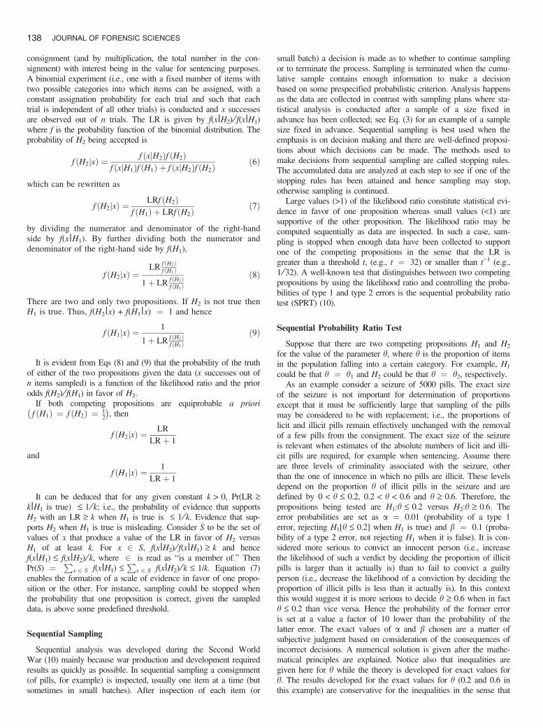
Consider the seizure of 5000 pills and propositions H1:h £ 0.2and H2:h ‡ 0.6; with a ¼ 0.01, b ¼ 0.1. As stated above, theinequalities for h may be replaced with equalities when developingthe test protocol. Insertion of the values h1 ¼ 0.2, h2 ¼ 0.6,a ¼ 0.01, and b ¼ 0.1 into Eqs (14)–(16) gives values for k1,k2, and k of )1.3, 2.8, and 0.4, respectively. Figure 1 illustrates theprocedure. The two parallel lines represent the lower and upperthresholds (k1 + kn, k2 + kn) where

k1 þ kn ¼ �1:3þ 0:4n

k2 þ kn ¼ 2:8þ 0:4n

Suppose the first five pills inspected in a sample were foundto be illicit. The line 2.8 + 0.4n is crossed and it can be decidedto act as if H2 is true (h ‡ 0.6).

TABLE 1—Probabilities of accepting a certain hypothesis.

LR>A (Accept H2) LR<B (Accept H1)

H1 is correct a 1)aH2 is correct 1)b b


This example may be used to illustrate the result that Pr(LR ‡k|H1) £ 1 ⁄k. For 5 ‘‘successes’’ out of 5 pills, theLR ¼ h5

2=h51 ¼ ð0:6=0:2Þ5 ¼ 35 ¼ 243 . Set k ¼ 243. Then

PrðLR � 243jH1Þ ¼ Prð5 successes out of 5 pills jh ¼ 0:2Þ¼ 0:25 ¼ 1=3125 < 1=243

Bayesian Approaches to Sample Size Determination for

Binary Responses

The work of Royall (9) was extended by De Santis (11) to aBayesian setting. De Santis used the LR and determined an appro-priate sample size to be one for which there was a large probabilityof observing strong, correct evidence while there was a small prob-ability of observing weak, misleading evidence. The probability ofobserving strong evidence is associated with the other two probabil-ities of observing weak and moderate evidence. As before (9),

thresholds need to be set in order to determine what constitutesstrong and weak evidence. The probability of accepting a certainproposition after data have been observed (Eq. [7]) may providesuch thresholds or Royall’s benchmarks

8; 32;18;

132

� �

might be used (9).Other Bayesian approaches determine the sample size as that for

which a function, such as the variance (12) of the posterior distri-bution of the characteristic of interest, h, satisfies some prespecifiedcriterion, e.g., the variance is less than a certain value. This wouldcorrespond to a requirement to estimate the characteristic to withina certain precision. Let T(h|xn) denote a function of the posteriordistribution of h whose performance is to be controlled. This is tobe carried out by the design of an experiment that will provide asample of size n, and xn denotes the number of members of thesample with the characteristic, where the subscript in this contextdenotes the sample size. Other examples of such functions are theaverage posterior interquartile range, the width of the highest pos-terior density (HPD) interval (13) (a procedure which considers theposterior density of h, f(h|x), and finds the shortest interval forwhich the probability that h lies in that interval is a predeterminedprobability, say 0.95) and the posterior probability of a certainproposition (14). Most Bayesian SSD techniques select the minimaln for chosen values of � (>0) and a (>0) (significance level) thatsatisfy either of the two following statements

E½TðhjxnÞ� � � ð17Þ

or

Pr½TðhjxnÞ=2R� � a ð18Þ

equivalently Pr½TðhjxnÞ 2 R� � 1� a ð19Þ

for an appropriate interval R, where =2 indicates ‘‘is not a mem-ber of.’’

Average Posterior Variance

In the examples that follow, the criterion that is used is the meanposterior variance where T(h|xn) ¼ var(h|xn). A reason for using

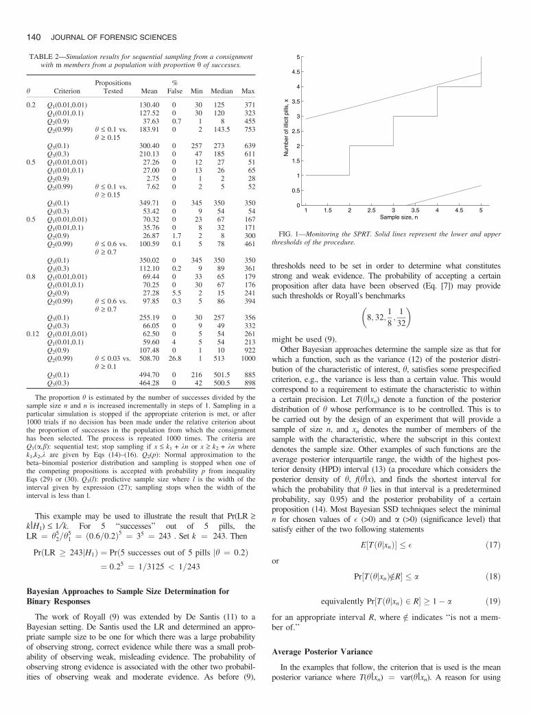
TABLE 2—Simulation results for sequential sampling from a consignmentwith m members from a population with proportion h of successes.

h CriterionPropositions

Tested Mean%

False Min Median Max

0.2 Q1(0.01,0.01) 130.40 0 30 125 371Q1(0.01,0.1) 127.52 0 30 120 323Q2(0.9) 37.63 0.7 1 8 455Q2(0.99) h £ 0.1 vs.

h ‡ 0.15183.91 0 2 143.5 753

Q3(0.1) 300.40 0 257 273 639Q3(0.3) 210.13 0 47 185 611

0.5 Q1(0.01,0.01) 27.26 0 12 27 51Q1(0.01,0.1) 27.00 0 13 26 65Q2(0.9) 2.75 0 1 2 28Q2(0.99) h £ 0.1 vs.

h ‡ 0.157.62 0 2 5 52

Q3(0.1) 349.71 0 345 350 350Q3(0.3) 53.42 0 9 54 54

0.5 Q1(0.01,0.01) 70.32 0 23 67 167Q1(0.01,0.1) 35.76 0 8 32 171Q2(0.9) 26.87 1.7 2 8 300Q2(0.99) h £ 0.6 vs.

h ‡ 0.7100.59 0.1 5 78 461

Q3(0.1) 350.02 0 345 350 350Q3(0.3) 112.10 0.2 9 89 361

0.8 Q1(0.01,0.01) 69.44 0 33 65 179Q1(0.01,0.1) 70.25 0 30 67 176Q2(0.9) 27.28 5.5 2 15 241Q2(0.99) h £ 0.6 vs.

h ‡ 0.797.85 0.3 5 86 394

Q3(0.1) 255.19 0 30 257 356Q3(0.3) 66.05 0 9 49 332

0.12 Q1(0.01,0.01) 62.50 0 5 54 261Q1(0.01,0.1) 59.60 4 5 54 213Q2(0.9) 107.48 0 1 10 922Q2(0.99) h £ 0.03 vs.

h ‡ 0.1508.70 26.8 1 513 1000

Q3(0.1) 494.70 0 216 501.5 885Q3(0.3) 464.28 0 42 500.5 898

The proportion h is estimated by the number of successes divided by thesample size n and n is increased incrementally in steps of 1. Sampling in aparticular simulation is stopped if the appropriate criterion is met, or after1000 trials if no decision has been made under the relative criterion aboutthe proportion of successes in the population from which the consignmenthas been selected. The process is repeated 1000 times. The criteria areQ1(a,b): sequential test; stop sampling if x £ k1 + kn or x ‡ k2 + kn wherek1,k2,k are given by Eqs (14)–(16). Q2(p): Normal approximation to thebeta–binomial posterior distribution and sampling is stopped when one ofthe competing propositions is accepted with probability p from inequalityEqs (29) or (30). Q3(l): predictive sample size where l is the width of theinterval given by expression (27); sampling stops when the width of theinterval is less than l.

1 1.5 2 2.5 3 3.5 4 4.5 50

0.5

1

1.5

2

2.5

3

3.5

4

4.5

5

Sample size, n

Num

ber

of il

licit

pills

, x

FIG. 1—Monitoring the SPRT. Solid lines represent the lower and upperthresholds of the procedure.


that function is its simplicity both in intuitive terms as it is an ana-logue of Cochran’s (1977) method (Eq. [2]) of determining thesample size as well as in mathematical terms as a beta conjugateprior can be used for h leading to a beta posterior with a mathe-matical expression for the variance (Eq. [49]). The mean posteriorvariance criterion finds the minimum n for which

E½varðhjxnÞ� � � ð20Þ

where � is some prespecified limit.

Predictive Sample Size Determination

When the consignment size m is known it is possible to deter-mine an appropriate sample size by estimation of the distributionof the number y of items that are illicit in the m)n units notinspected (15). This is in contrast to the estimation of h, a propor-tion. The reason for the contrast may be explained in the contextof a super-population. The consignment may itself be considered asa sample from a larger population, known as a super-population(such as the overall output of a drug factory), within which hdenotes the proportion of items that are illicit. This proportion maybe estimated from a sample from the consignment under inspectionfrom the super-population. The super-population may be conceptu-ally infinite, for example as the total output of the drug factorymay be unknown other than it is extremely large.

The approach that estimates y directly is an alternative to consid-eration of properties of h, the proportion of illicit items in a con-signment and, by extension, the super-population. A beta(m1,m2)prior for h is considered which yields an updated posterior distribu-tion for h of beta(m1 + x, n ) x + m2). The so-called predictive dis-tribution of Y is then given by

PrðY ¼ yjxÞ ¼Z 1

0PrðY ¼ yjhÞf ðhjxÞdh ð21Þ

where f(h|x) is the posterior distribution of h (beta(m1 + x,n ) x + m2)) and

PrðY ¼ yjhÞ ¼ m� n

y

� �hyð1� hÞm�n�y ð22Þ

It can be shown that

PrðY ¼ yjxÞ ¼ m� n

y

� �Bðm1 þ xþ y;m� x� yþ m2Þ

Bðm1 þ x; n� xþ m2Þ;

y ¼ 0; . . . ;m� n

a beta–binomial distribution with parameters (m1 + x + y,m ) x ) y + m2) (5). It is necessary to work with the cumulativedistribution function in order to determine probabilities that Y isgreater than a certain value and hence the total size of the illicitpart of the consignment is greater than a certain value. If m islarge this will involve the summation of many values. It is com-putationally intensive but feasible with computer software pack-ages such as MATLAB. If a suitable computer package is notavailable an alternative option is to use the beta distribution (5).Alternatively, the normal approximation to the beta–binomialdistribution may be used (5) where the mean l is given by

l ¼ ðm� nÞðxþ m1Þnþ m1 þ m2

ð23Þ

and the variance r2 is given by

r2 ¼ ðm� nÞðxþ m1Þðn� xþ m2Þðmþ m1 þ m2Þðnþ m1 þ m2Þ2ðnþ m1 þ m2 þ 1Þ

ð24Þ

The sample size may then be determined as the smallest n, forgiven m and h, such that

PrðY � cm� xnÞ � 1� a ð25Þ

where PrðY � y0Þ ¼Py0

y¼0 f ðyjxnÞ; xn is the number of illicititems, and c, 0 £ c £ 1, is a prespecified threshold. Similarly,there may be interest in satisfying a criterion of the form

PrðY � cm� xnÞ � 1� a ð26Þ

Note that (xn + y) ⁄ m is the proportion of illicit pills in the con-signment and hence y £ cm ) xn is equivalent to the proportion(xn + y) ⁄ m £ c. Hence, the above inequalities Eqs (25) and (26)denote probabilistic bounds on the sample sizes. In summary,after n and xn have been observed and for given m, a Normalapproximation may be used to determine the total number of illi-cit pills in the consignment, with mean and variance given byEqs (23) and (24), respectively. Therefore, in an extreme sce-nario and for significance level a, either ya or y1)a illicit pillsare found in the remaining m ) n trials, depending on which ofthe propositions Eqs (25) and (26) ‘‘Y less than a certain value’’or ‘‘Y greater than a certain value’’ are to be tested, withya ¼ l + zar, U(za) ¼ a, U(z1)a) ¼ 1 ) a, where U denotesthe cumulative distribution of the standard normal distributionand 0 £ a £ 0.5. Therefore the 100(1 ) a)% interval for the pro-portion, h, of illicit pills in the population is the interval

x þ l þ zarm

;x þ l þ z1�ar

m

� �where the subscript n has been dropped from the x for ease ofnotation. This method can be used both for making an infer-ence from the sample to the population and for a sequentialsampling scheme where sampling is stopped when the proba-bility interval

xþ lþ z1�arm

;xþ lþ zar

m

� �ð27Þ

has a width less than a certain value l or when the estimatedprobability, (x + y) ⁄ m, of an illicit pill in the population fallsinto a prespecified interval. In simulation results reported inTable 2 the first method is used and denoted by Q3(l). Theremay be cases where there is interest only in rejecting one of thetwo competing propositions without any need for an accurateestimation of h. A requirement to control the width of the prob-ability interval may result in a big sample size especially if h isclose to 0.5. Alternatively, sampling may be stopped whenalong with the upper and lower bounds satisfying either H1 orH2, a specific number of sampling units has been inspected,e.g., 10 or 20.

Items are tested sequentially and stopping rules are defined. Forexample, a rule may be to stop if the proportion of illicit drugs inthe consignment is estimated to exceed 60%. Alternatively, a rulemay be to stop if the proportion in the consignment is estimated tobe below 20%. For intermediate values as well as for values thatlie both in the acceptance and rejection regions [i.e., (x + l +zar) ⁄m lies in the lower region and (x + l + z1)ar) ⁄m in the upperregion] sampling is continued until only one of the two criteria issatisfied, or an upper limit, e.g., 1000, is reached when it is decidedto behave as if 0.2 < h < 0.6.

Suppose a sample of six units (n ¼ 6) from a seizure ofm ¼ 5000 pills is taken and there are six successes (i.e., the num-ber x of illicit pills equals the sample size six). The beta prioris taken to be beta(1,1). The mean l (Eq. [23]) of the posterior


beta–binomial distribution is 4369.75, a proportion 87.4% of 5000.The variance r2 (Eq. [24]) is 550.9782. The significance level a istaken to be 0.01 so that za ¼ )2.3263 and z1)a ¼ 2.3263. Then

ya ¼ l þ zar ¼ 3088:01 andx þ ya

m¼ 0:62 > 0:6

i.e., the probability that the true proportion of illicit pills isgreater than 0.62 is 0.99. Sampling is stopped with the decisionto act as if the seizure is contaminated to a degree larger than60%.

Criterion for Sample Size Calculations for Proportions with

Binary Responses

Return now to consideration of a population proportion ratherthan a number of items in a consignment. A criterion where thescientist wants to be 100p% certain that at least 100l% of aconsignment contains drugs when all n units in the sample containillicit drugs is provided by (5). As an example, when p ¼ 0.95and l ¼ 0.5, the criterion can be written mathematically as

Prðh > 0:5jm1 þ n; m2Þ ¼R 1

0:5 hnþm1�1ð1� hÞm2�1 dh

Bðnþ m1; m2Þ� 0:95 ð28Þ

A context different from that of drugs is that of the inspection ofa hand for gunshot residue. A person is suspected of firing a gun.A sample of particles is taken from his hands and wrists. Samplingof particles can stop when the first particle of gunshot residue isfound. The problem is to determine a number for the particles thatshould be sampled before stopping if no particle has been found.This number can be determined by using a criterion that the scien-tist wishes to be 100p% certain that the probability there is no gun-shot residue present is at least 100l%. In this context possiblevalues for p and l are 0.95 and 0.99, say. Consider m1 ¼ m2 ¼ 1(the uniform prior mentioned in the Appendix and the skepticalprior of the following section) in Eq. (28). Denote the probabilitythat no gunshot residue is present by h. Then the criterion may bewritten mathematically as

Prðh > 0:99j1þ n; 1Þ ¼R 1

0:99 hn dh

Bðnþ 1; 1Þ ¼ ðnþ 1ÞZ 1

0:99hndh � 0:95

(Note that (1 ) h)m2 ) 1 ¼ (1 ) h)0 ¼ 1 when m2 ¼ 1.) Thesample size n is chosen as the smallest integer that satisfies thisinequality. This value is determined as follows.

ðnþ 1ÞZ 1

0:99hndh � 0:95) ½hnþ1�10:99 � 0:95

) 1� 0:99nþ1 � 0:95

) 0:99nþ1 � 0:05

) ðnþ 1Þ � logð0:05Þ= logð0:99Þ) n � 297:07

Thus if the scientist wishes to be 95% certain that the probabil-ity there is no gunshot residue present is at least 99% then justunder 300 particles have to be examined. This is a very strictcriterion and leads to a large sample size which may not bepossible to achieve in practice. An alternative approach is toconsider the inference that may be made if a fixed sample sizeis chosen and no particles of gunshot residue are found in thatsample. For example, if the sample size n is chosen to be 10,then it can be shown that it is 50% certain that the probability

no gunshot residue is present is greater than 0.94 and approxi-mately 70% certain that the probability no gunshot residue ispresent is greater than 0.90.

It is suggested in Ref. (16) that a community of priors represent-ing skeptical, enthusiastic, and weak prior beliefs should be consid-ered in every experiment and that all three beliefs should lead tothe same conclusion in order to make inference about the targetpopulation. Parameter values m1 and m2 need to be found for thebeta distribution that will represent the three different beliefs. Suchparameters can be m1 ¼ 1 and m2 ¼ 1 for the skeptical belief,m1 ¼ 10 and m2 ¼ 1 for the enthusiastic belief, and m1 ¼ 1 andm2 ¼ 10 for the weak belief. The sample sizes following thismethod and for p ¼ 0.95 and l ¼ 0.5 are 4, 1, and 18, respec-tively. The last two figures show that an enthusiastic prior beliefrequires little extra evidence to satisfy the criterion and a weakprior belief requires much extra evidence. The results also illustratehow previous knowledge can lead to variations in the sample sizeand hence the cost of analysis. However, such a criterion should betested sequentially because if the first item sampled is ‘‘negative’’sampling has to continue beyond these values. Application of asequential sampling scheme enables the prior beliefs to be updatedas samples are investigated.

A Bayesian Two-Sided Sequential Criterion

Suppose that there are two competing propositions H1:h £ h‘and H2:h ‡ hu, (hu > h‘). These two propositions are tested sequen-tially. First, some stopping rules are defined. It is decided to act asif H1 is true if there is at least a p1% probability that h < h‘ and toact as if H2 is true if there is a p2% probability that h > hu. Sam-pling is continued until either of these rules is satisfied. Assume abeta prior, beta(m1,m2), for h. The posterior distribution after theinspection of the ith sampling unit is also a beta distribution withparameters m1 + xi and m2 + i ) xi where xi is the number of ‘‘suc-cesses’’ up to the ith inspected sampling unit, and h is the probabil-ity of a success.

Therefore, sampling is stopped, either when

Prðh < h‘jm1 þ xi; m2 þ i� xiÞ

¼R h‘

0 hm1þxi�1ð1� hÞm2þi�xi�1 dh

Bðm1 þ xi; m2 þ i� xiÞ� p1 ð29Þ

or when

Prðh > hujm1 þ xi; m2 þ i� xiÞ

¼R 1

huhm1þxi�1ð1� hÞm2þi�xi�1 dh

Bðm1 þ xi; m2 þ i� xiÞ� p2 ð30Þ

For hu ¼ 0.5 and p2 ¼ 0.95, Eq. (30) is equivalent to the cri-terion suggested in Eq. (28) when only ‘‘successes’’ areobserved (xi ¼ i).

The Use of Historical Data for Determination of the Sample

Size with Power Priors

Prior information from historical data may lead to a substantialsaving of time and financial resources. The so-called power priorsfor the incorporation of information from previous studies wereused in Ref. (17) to form a suitable prior for a current study.

Consider the previous example with 5000 illicit pills. There areno historical data from the suspect but there are historical dataassociated with the conditions under which the seizure is captured.For instance, there may be information about the location where


the seizure has been found (e.g., hidden in a boat in transit) orthere may be historical data from circumstantial evidence associatedwith the suspect (e.g., previous convictions, illegal possession ofweapons, fake transport or other papers, possession of largeamounts of money). Suppose now that the seizure was caughtunder circumstances similar to those of a previous seizure of illicitpills in which 25 pills were analyzed and all of them were foundto be illicit. These 25 pills may be used as historical data. The wayin which the data may be used is explained in general and then thisparticular example is developed.

Previous studies should be similar to the current one in that thesame likelihood should be able to be used for inference about thecharacteristics of interest. Suppose that the data (sample size andthe number of illicit drugs in the sample) from a previous similarstudy are denoted by D0. The power prior fp/(h|D0) that will beused in the current study is

f pðhjD0Þ / LðhjD0Þf0 f ðhÞ ð31Þ

where h is the parameter of interest, superscript ‘‘p’’ denotespower prior, L denotes the likelihood and f0 is a coefficient,between 0 and 1, weighting the effect of historical data on thecurrent study and f(h) is a prior before consideration of the his-torical data. As f0 fi 1 the standard posterior of (h|D0) isobtained whereas as f0 fi 0 the prior that would have beenused in the absence of historical data is obtained. Intermediatevalues of f0 are associated with different weights for historicaldata, the closer f0 is to 1, the stronger the belief in the validityand relevance to the case in hand of the historical data.

Suppose a binomial experiment is conducted. A beta prior,beta(m1,m2), is considered. There is also some information from asimilar experiment conducted in the past. The likelihood obtainedfrom that previous experiment is

LðhjD0Þ ¼n0

x0

� �hx0ð1 � hÞn0�x0

with n denoting the sample size, x the number of successes andindex 0 denoting reference to a previous study; see Eq. (1) with(n0,x0) ¼ D0. The power prior is a beta with parameters(f0x0 + m1,f0(n0 ) x0) + m2),

f pðhjD0Þ / LðhjD0Þf0 f ðhÞ

¼ n0

x0

� �hx0ð1� hÞn0�x0

� �f0

hm1�1ð1� hÞm2�1

/ hf0x0þm1�1ð1� hÞðn0�x0Þf0þm2�1 ð32Þ

Suppose that instead of one, there are multiple (G) prior indepen-dent sets of results from historical data, denoted byD0 ¼ (D01,…,D0G)¢. Each previous case is given a weight fgf0

(g ¼ 1,…,G) where f0 is the overall weight that is assigned to pre-vious data and fg(>0) is the specific weight assigned to case g andPG

g¼1 fg ¼ 1. The power prior in such a situation is defined as

f pðhjD0Þ / ðLðhjD01Þf1 � � � LðhjD0GÞfGÞf0 f ðhÞ ð33Þ

Power priors have been combined with results from simulations,conducted under experimental conditions, to determine appropriatesample sizes (18). For various sample sizes, values were generatedfrom the power prior distribution Eqs (32)–(33) of the parameter ofinterest and the information in the posterior distribution was sum-marized by some statistic such as the posterior variance. Then thevalue of that statistic for various sample sizes was plotted against

the corresponding sample sizes. A minimal sample size was chosenso that a certain criterion was met. Let T(h|xn) denote the statisticfrom a sample of size n from the posterior distribution of h, givendata xn, whose performance is to be controlled by appropriate sam-pling. Examples of such statistics are, as before, the posterior vari-ance (12), the mean posterior interquartile range and the width ofthe HPD interval (13). De Santis’ method (18) for estimation of theprecision of a statistic T in a power prior where the statistic cannotbe determined analytically consists of the following steps:

• Draw a number, let it be b, of h*s ðh�1; . . . ; h�bÞ from the powerprior distribution f p(h*|D0) with given values n0, x0, f0, m1, andm2. (The symbol * denotes a simulated value.) A typical valueof b may be 1000.

• Draw, for each h*, a simulated sample x�n of size n from thesampling distribution f(x|h*), to give a likelihood Lðhjx�nÞ.

• Compute f ðhjx�n;D0Þ / Lðhjx�nÞf pðh�jD0Þ for each of the bgenerated samples.

• Compute Tðhjx�nÞ for each of the b generated samples.• Approximate Pr(T(h|xn)) 2 A with the proportion of the b gen-

erated samples Tðhjx�nÞ that belong to the set A. Similarly,E[T(h|xn)] is estimated by the sample arithmetic mean of the bgenerated values Tðhjx�nÞ and varðTðhjx�nÞ by the samplevariance.

This method, with the same b, is applied repeatedly to larger val-ues of n until the required criterion is met, for example that theposterior standard error of the statistic T is less than a certain value.This gives the sample size to be used in future cases for which thecorresponding power prior is relevant.

Suppose the posterior variance for a sample of size n because ofits relative simplicity is chosen as the statistic T of the posteriordistribution. Assume a beta prior and a binomial sample. Thevariance of the beta posterior (or power prior) described here isgiven by ðm�1m�2Þ=ððm�1 þ m�2Þ

2ðm�1 þ m�2 þ 1ÞÞ where m�1 ¼ f0x0þm1 þ x� and m�2 ¼ f0ðn0 � x0Þ þ m2 þ n � x�. This is dividedby the sample size n and then the square root is taken to obtain theposterior standard error. The simulation process is not required hereas the posterior standard error can be determined analytically.

The sample size could then be chosen as the minimum samplesize for which the posterior standard error is lower than some pre-specified value, 0.01 or 0.05, for example. In practice by drawingplots of the posterior standard error against the sample size thebehavior of the procedure can be monitored by observing decreasesin the posterior standard error as the sample size increases anddetermining the appropriate sample size as that one after which theposterior standard error decreases only slightly. A crucial aspect ofthe power prior approach is the choice of the weight f0 given tothe previous study. Optimal sample sizes are decreasing functionsof f0 as the less weight that is given to a previous, similar, studythe more uncertainty there is about the current study. The majoradvantage of this method is its simplicity and the fact that itenables numerous scenarios to be considered without any constraintof time or finance as everything is based on the previous study andon simulated results.

Consider the consignment of 5000 illicit pills withn0 ¼ x0 ¼ 25. A beta(1,1) prior is taken. Figure 2 shows themean posterior standard error, using De Santis’ method (18), forvarious weights f0 given to the previous study, as the sample sizeincreases. For large values of n the weight given to the previousstudy is of little importance. A sample size of 60 seems adequateregardless of the weight attached to the previous study.

If a large degree of trust (e.g., f0 ¼ 0.8) is permitted for thehistorical data, a sample size of 10 yields a posterior standard error


smaller than 0.01 and that would lead to a considerable saving oftime and financial resources. This can be verified numerically.First, consider f0 ¼ 0.8, n0 ¼ x0 ¼ 25, m1 ¼ m2 ¼ 1,n ¼ x* ¼ 10. Then m�1 ¼ 31 and m�2 ¼ 1. The posterior vari-ance ¼ 31/(322·33).0.0302882 and the posterior standard errorequals 0:030288=

ffiffiffinp¼ 0:0096 ¼ 0:01, to two decimal places,

when n ¼ 10. Second, consider f0 ¼ 0. Values ofn ¼ x* ¼ 10 give a posterior standard error of 0.024 and valuesof n ¼ x* ¼ 20 give a posterior standard error of 0.01. Thus,without the historical data, the sample size required to provide thesame standard error is bigger by a factor of two.

If there are no historical data available, a similar approach maybe followed by investigating a fraction of the data as if it were his-torical data. This fraction should be given full weight (f0 ¼ 1) asit is part of the data. By applying the power prior approach, afterinspecting an initial fraction of the data, the extra samples thatshould be taken may be determined.

Comparison by Simulations of Methods for Sample Size

Determination for Binomial Populations

So far, three sequential methods have been suggested for SSDfor binomial populations. The results of comparisons of their per-formances using simulations are presented in Table 2. The firstmethod is the SPRT which, in the simulations presented in Table 2,is denoted by Q1(a, b) where a and b are the probabilities of type1 and type 2 error, respectively. The other two methods are Bayes-ian and they employ the conjugacy property of the beta distributionwith respect to binomial sampling to obtain a closed-form posterior(beta–binomial). In all simulations conducted a beta(1,1) prior wasassumed for the probability of ‘‘success’’ h. One method uses onlythe posterior distribution of the population parameter and samplingis stopped when one of the competing propositions is accepted witha certain probability (either inequality Eq. [29] or inequality Eq.[30] is satisfied). This two-sided sequential criterion is denoted byQ2(p) in Table 2 with p denoting the probability that one of thecompeting propositions is accepted. The last method combinesinformation both from the inspected units, up to a specific point,and from the predictive distribution of the units not inspected. Thecriterion Q3(l) is used and sampling is stopped when the predictiveprobability interval, expression (27), is less than l in width.

The analysis of random samples is used for evaluating the differ-ent criteria. The results presented in Table 2 are obtained from1000 random samples. All three methods [Q1(a, b), Q2(p), Q3(l)]are compared on the same simulated samples.

The Q1 criterion (SPRT) yields the most stable results even ifvery small type 1 and type 2 error probabilities (a and b) are used.Also, the mean sample size is always close to the median (slightlylarger), although the distance of the maximum sample to mediansample size is much larger than the corresponding distance of themedian sample size to the minimum one. Very large sample sizeswere observed in less than 0.5% of the samples.

The Q2 criterion (two-sided sequential criterion) is very muchdependent on the probability p defined a priori for selecting one ofthe two competing propositions. It gives very small sample sizeswhen the true population proportion h is far away from both h1

and h2 or when h1 is not very close to h2. The population propor-tion is not known in advance and when it is close to either h1 orh2 the sample size required is increased considerably. Also the dis-tribution of the sample size is skewed to the right and there is aconsiderable probability of obtaining a large sample size. There arealso cases where the entirety of the samples (maximum equals1000) is investigated without reaching any conclusion.

The Q3 criterion is dependent on the maximum width of theinterval that is specified. For values of h close to 0.5, with a popu-lation size equal to 1000 and for a maximum permitted width ofthe interval equal to 0.1, the sample size required is around 350with little variation. An increase in the maximum permitted widthof the interval leads, not surprisingly, to a reduction in the requiredsample size.

If there is no restriction on the width of the interval, the methodmay lead to sample sizes of just one unit with a high probability ofaccepting the wrong proposition. Alternatively, the restrictionplaced on the width of the probability interval for h can beremoved and a restriction instead placed on the number of sam-pling units, e.g., to be at least equal to 20. This method leads tosmall sample sizes with zero probability of accepting the wrongproposition in all cases presented in Table 2 with the exception ofthe last case (h ¼ 0.12 and h £ 0.03 vs. h ‡ 0.1) which gives aprobability very close to 0.6 (0.571). From various simulations,under different scenarios, the conclusion is that when h is veryclose to either of the propositions being tested there is a high prob-ability of obtaining misleading results.

Multinomial Sampling

Previous examples have considered a binary response. There aresituations in forensic science where a consignment may have morethan two categories of items in it. For example, in a drug case aconsignment of pills may have three categories such as licit,ecstasy, and LSD and several other examples have been given inthe introduction. In all of these examples the problem is to deter-mine the size of the sample needed in order to estimate the propor-tions of each category.

There are extensions to the ideas presented here for which fur-ther work is needed. In the examples in the previous paragraph thenumber of categories is assumed known. If this is not the case thena different approach is needed to estimate the number of categoriesas well as the proportion of each. Also, even if the number of cate-gories is known, another problem is to determine how big a sam-ple is needed in order to ensure there is at least one item in thesample from each type. This problem has already been consideredabove in the example of gunshot residue where the sample sizewas determined in order to have a certain probability of detecting

0 20 40 60 80 1000

0.02

0.04

0.06

0.08

0.1

0.12

Sample size, n

Ave

rage

pos

terio

r st

anda

rd e

rror

0.2

0.5

0.8

FIG. 2—Graphs of the sample size versus the average posterior standarderror for various weights assigned to historical data [f0 ¼ (0.2,0.5,0.8)]for inspection of a consignment of 5000 pills, each of which is either licitor illicit. Historical data are available of a sample of size n0 ¼ 25 pills inwhich all pills were illicit (x0 ¼ 25).


the presence of a particle of gunshot residue if a certain proportionof the total number of particles were gunshot residue. The problemcan be extended further. Consider a collection of glass fragments.The problem is to determine the size of the sample that is neededto ensure there is at least one item in the sample from each cate-gory of glass.

Study of the problem of estimation of proportions when there aremore than two categories requires a generalization of the situationin which there is a binary response and for which a binomial distri-bution is appropriate. The binomial distribution models the variationfor the number of outcomes of a particular type in a sequence ofindependent trials where there are only two possible, mutuallyexclusive outcomes and the probability of a particular outcome isconstant and fixed from trial to trial. The generalization models thevariation for the number of outcomes of a particular type in asequence of independent trials where there are several possiblemutually exclusive outcomes and the probability of a particular out-come is constant and fixed from trial to trial. The distribution whichgeneralizes the binomial distribution is the multinomial distribution.The probability of a success in a binomial context is denoted h withthe corresponding probability of a failure denoted (1 ) h). Consider,now, k categories, where k ‡ 2 and k ¼ 2 corresponds to the bino-mial context. The parameters of the multinomial distribution may bedenoted h ¼ (h1,…,hk)

¢, wherePk

j¼1 hj ¼ 1 and h1,…,hk > 0.The distribution is itself denoted Mn(h1,…,hk) where Mn is shortfor ‘‘multinomial.’’ The probability function for x is given by

Prðxjn; h1; . . . ; hkÞ ¼n!Qk

j¼1 hxijQk

j¼1 xj!ð34Þ

where

Xk

j¼1

hj ¼ 1;Xk

j¼1

xj ¼ n ð35Þ

It is desired to obtain the set of k intervals Sj, j ¼ 1,…,k, ofthe shortest length such that

Pr\kj¼1

ðhj 2 SjÞ( )

� 1� a ð36Þ

The sample proportions are denoted by the vectorh ¼ ðh1; . . . ; hkÞ0 where hj ¼ xj=n. An example for the inter-vals Sj may be those defined by the absolute difference of theestimates hj and the corresponding parameters hj, and a criterionthat the absolute difference be less than dj, j ¼ 1,…,k. It isrequired that the probability will be at least 1)a that all of theestimated proportions hj will simultaneously be within dj of thetrue population proportions hj, that is,

Pr\kj¼1

jhj � hjj � dj

( )� 1� a ð37Þ

It is assumed that the population is large enough for finite popu-lation correction factors to be ignored and that sample sizes arelarge enough for the normal approximation to be used. The sampleproportions h converge asymptotically to a so-called degeneratemultivariate normal distribution

h � N h;Vð Þ ð38Þ

where V ¼ (1/n) (diag(h))hh¢) is the k · k covariance matrixand diag denotes a diagonal matrix (i.e., a matrix in whichthe diagonal terms are the components (h1,…,hk) and the

off-diagonal terms are zero. The covariance matrix V has theelements (1 ⁄ n)hj(1 ) hj) on its main diagonal and off-diagonalelements )(1 ⁄ n)hj1

hj2for j1 „ j2 and j1, j2 ¼ 1,…,k. This is a

singular covariance matrix (i.e., one whose inverse does notexist) of dimension k ) 1 due to the restriction

Pkj¼1 hj ¼ 1,

hence the term ‘‘degenerate.’’A method for constructing simultaneous confidence intervals for

multinomial proportions is presented in Ref. (19). The methodassumes that nhj is large enough (at least 5) for the square of thePearson’s residual

Xk

j¼1

ðxj � nhjÞ2

nhj

to be chi-squared distributed with k ) 1 degrees of freedom.This result was improved through the construction of less con-servative confidence intervals (19). This improved method wasbased on the normal approximation for a binomial proportionand used Bonferroni’s inequality to put a bound on the probabil-ity that all of the intervals would be simultaneously correct.Neither Goodman (20) nor Quesenberry and Hurst (19)addressed the problem of the sample size. Goodman’s (20)equation for a (1 ) a)% confidence interval for hi is

hj � z a2k

ffiffiffiffiffiffiffiffiffiffiffiffiffiffiffiffiffiffiffiffihjð1� hjÞ

n

r; hj þ z a

2k


n

r !ð39Þ

Angers (21) noted that because the distribution of hj convergesasymptotically to a degenerate multivariate normal distribution witha singular variance covariance matrix of rank k ) 1 the correct(1 ) a)% confidence interval for hj is

hj � z a2ðk�1Þ


n

r; hj þ z a

2ðk�1Þ


n

r !ð40Þ

The probability aj, that the sample estimate hj is further than dj

from hj is given by the normal approximation to a binomialproportion

aj ¼ Prðjhj � hjj > djÞ ’ 2ðk � 1Þ 1� Udj

ffiffiffinpffiffiffiffiffiffiffiffiffiffiffiffiffiffiffiffiffiffiffiffi

hjð1� hjÞp ! !

ð41Þ

The smaller the ajs the larger the sample size required in orderto attain them. A decrease in aj implies a decrease in

1 � Udj

ffiffiffinpffiffiffiffiffiffiffiffiffiffiffiffiffiffiffiffiffiffiffiffiffi

hjð1 � hjÞp ! !

which arises from an increase in n, for unchanged dj and h. Inthe multinomial setting, two simple methods for deriving theappropriate sample size are as follows:

1 Assume the parameter vector h ¼ (h1,…,hk)¢ is known. Select

a sample size n, observe x1,…,xk, calculate hj; j ¼ 1; . . . ; k andcompute

Pkj¼1 aj for given dj, j ¼ 1,…,k. If

Pkj¼1 aj < a,

repeat with a smaller value of n. Otherwise, repeat with a largervalue for n until the smallest n is found such that

Pkj¼1 aj � a.

The algorithm is usually initialized with sample size equal toone and the sample size is incremented gradually by one unit ata time until

Pkj¼1 aj � a. This method is employed in Ref.

(22) where the vector h was considered known and the sample


size for obtaining confidence intervals of specified lengths wasto be determined. An obvious disadvantage of this method isthat the vector of proportions attributed to each category isnever known in advance.

2 The second method is to carry out the first procedure with allpossible parameter values to determine the parameter vectorwhich gives the largest sample size and use this sample size.This method was applied by Thompson (23) and the form ofthe worst case scenario was established. More specifically,Thompson proved that the worst case scenario for a multinomialdistribution occurs when k ) h (0 £ h £ k) proportions are equalto zero and the remaining h have probability h)1. If, for a casewith k categories, zero proportions for k ) h of the categoriesare observed the dimensionality of the data is reduced by k ) h.Zero observations for a category are taken to imply the trueprobability for the category is zero. For example if there is onecategory with zero frequency this means that the appropriatesample size is estimated considering a vector of equal probabili-ties assigned to k ) 1 categories. A disadvantage of this methodis that it might lead to unnecessarily large samples especiallywhen there are categories with high or low proportions and,therefore, small variances.

Table 3 gives the appropriate sample sizes needed for a trinomialexperiment so that the probability that one or more of the k esti-mates of proportions hj, j ¼ 1,…,k is outside an interval of length2d ¼ 2 · 0.05 ¼ 0.1 centered on the true, unknown, proportionh, will be less than or equal to a. For larger numbers of categories,the sample sizes are the same as with k ¼ 4 as the worst casescenario gives zero frequencies to many cells leaving only fourwith nonzero and equal probabilities. This is a restriction of theworst case scenario defined by Thompson.

The effect on sample size of assuming the worst case can beillustrated with other choices of the set of proportions. Considerk ¼ 3 and a ¼ 0.05. First, assume the true set of proportions ish ¼ (0.2,0.3,0.5)¢ rather than the worst case scenario. In that casethe sample size reduces from 624 (Table 3) to 593. If the seth ¼ (0.05,0.05,0.9)¢ is considered the necessary sample size isreduced to 182. Assumption of the worst case scenario leads to amuch larger sample size than necessary, with a consequent unnec-essary expenditure of resources. An alternative Bayesian procedureis shown to reduce the sample size considerably.

Bayesian techniques for SSD

Given a multinomial likelihood and a Dirichlet prior (Eq. [49])in the Appendix, the posterior distribution of the parameter vectorh is also a Dirichlet distribution

This posterior distribution can be approximated by the singularmultivariate normal distribution with mean vector l and variance–covariance matrix V. Then, it can be shown that (1)

T2 ¼ nþXk

j¼1

mj þ 1

!ðh� lÞ0V�ðh� lÞ � v2

k�1 ð42Þ

where v2k�1 denotes the chi-squared distribution with (k ) 1)

degrees of freedom, V) is the generalized inverse of V (see theAppendix for an explanation of a generalized inverse) and(m1,…,mk) are the prior parameters of the Dirichlet distribution.The sample size may be estimated using the requirementPr[T2 £ d2] ¼ 1 ) a that leads to the rule

nþXk

j¼1

mj þ 1 � v2k�1;a=d2 ð43Þ

where d2 ¼ (h ) l)¢V)(h ) l) is an ellipsoid in (k ) 1)-dimen-sional space, centered on l and v2

k�1;a denotes the percentagepoint of v2

k�1 such that for a random variable X2 with a v2k�1 distri-

bution PrðX2 > v2k� 1;aÞ ¼ a. Thus, from Eq. (43) a value for n

may be obtained (1). Note, although, that the choice of d and thechoice of parameters for the prior distribution both affect thechoice of sample size. Note that for large values of the priorparameters, and hence large

Pkj¼1 mj, one obtains smaller sample

sizes that in extreme cases may even become negative. A negativeresult implies that our prior beliefs are so strong that there is noneed to collect more data. The choice of n such thatn � v2

k�1;a=d2 is an appropriate conservative choice.

Power Priors for Multinomial Experiments

The use of historical data for determining the sample size usingpower priors for beta and binomial distributions can be extended tomultinomial data by using a Dirichlet prior for the parameters ofinterest.

Suppose a multinomial likelihood from a previous experimentleads to a Dirichlet power prior. More specifically, a Dirichlet priorwith parameters v ¼ (v1,…,vk) is combined with data (x01,…,x0k)from an experiment subsequent to the choice of prior but beforethe planned experiment. These data are given a weight f0. TheDirichlet power prior is then

f ðh1; . . . ; hkjvÞ /Yk

j¼1

hx0j

j

!f0Yk

j¼1

hvj�1j ¼

Yk

j¼1

hf0x0jþvj�1j

The power prior, combined with current data (x1,…,xk) yields aDirichlet posterior with parameters (f0x0j + xj+vj; i ¼ 1,…,k).The current data are not known in advance and a simulation-based approach, as that presented earlier in the context of thebeta distribution, is used to determine the sample size as that forwhich a function of the posterior distribution satisfies a prespec-ified threshold. Such a threshold may be the trace of the poster-ior covariance matrix (sum of parameter variances) or the sumof the posterior standard deviations. The parameters of theDirichlet posterior distribution are v�j ¼ f0x0j þ xj þ vj. Letv�0 ¼

Pkj¼1 v�j . The posterior covariance matrix has variances

varðxjjv�Þ ¼v�j ðv�0 � v�j Þv2

0ðv0 þ 1Þ ¼ njj

and covariances

TABLE 3—Appropriate sample sizes n using Thompson’s method(d ¼ 0.05) which assumes the worst assignment of proportions,

h1 ¼ … ¼ hk for various significance probabilities a and numbers k ofcategories such that the probability one or more of the estimates of theindividual category proportions are outside the intervals of length 2d

centered on the true, unknown, proportions h1,…,hk.

a n k

0.1 510 30.05 624 30.025 748 30.02 788 30.01 915 30.1 574 40.05 684 40.01 946 4


Cðxj1 ; xj2 jv�Þ ¼�v�j1 v�j2

v20ðv0 þ 1Þ ¼ nj1j2 ¼ nj2j1

where v� ¼ ðm�1; . . . ; m�kÞ0.

Suppose that there are historical data of n0 ¼ 100 observationsfrom a trinomial population with 20 observations falling in the firstcategory, 30 observations falling in the second category, and 50observations falling in the third category [x0 ¼ (20, 30, 50)]. Thecriterion for the choice of sample size is to choose as that size ofsample, the value for which the sum of the posterior standard devi-ations for the three categories is less than some prespecified value.Figure 3 plots the sample size for the current data versus the sumof the posterior standard deviations for various weights assigned tohistorical data. It can be seen that large sample sizes are needed,even for f0 ¼ 0.8, to provide estimates of the trinomial propor-tions in which the sum of the posterior standard deviations is lessthan 0.1.

Ternary Diagrams

Ternary diagrams are very popular in the geochemical sciences(24) and have been extensively used to represent the relative per-centages of three components as points in an equilateral triangle. Anecessary requirement for the construction of such a diagram is thatthe three components should sum to a fixed amount, for example,to 1 if proportions are being used or to 100 if percentages are beingused. This requirement places the restriction that once two of thecomponents are known the other is obtained by subtracting thesum of the two known components from the fixed amount. Hence,only two out of the three components are freely selected reducingthe dimension of the problem from three to two. Therefore, whilstternary diagrams provide a visual representation of apparentlythree-dimensional data, they are able to be plotted in two dimen-sions which eases interpretation. A ternary plot may be representedas an equilateral triangle as shown in Fig. 4.

Consider a trinomial experiment. Each subject gives only oneresponse but the cumulative proportion of each category may beseen as a form of compositional data as the sum of these is a con-stant (100%). This is illustrated in Table 4 where the cumulativepercentages, up to any number of subjects, may be seen as acomposition.

A brief discussion of the construction of such a diagram is given.Figure 5 shows the increments along the first axis. If the composi-tion of the first element is 0.1 then that element would lie on theline that corresponds to 0.1 in Fig. 5. All elements on that line referto two different combinations of the other two variables whichshould sum to 0.9.

The representation of the point (0.2, 0.3, 0.5) on a ternary dia-gram is shown in Fig. 6. Approximation of the multinomial proba-bility by a multivariate normal (Eq. [38]) enables the constructionof ellipsoidal contours of any precision. Figure 7 shows a 95%probability ellipse contour. The area E under the ellipse is given asthe product

0 50 100 150 2000.08

0.1

0.12

0.14

0.16

0.18

0.2

0.22

0.24

0.26

0.28

Sample size

Sum

of p

oste

rior

stan

dard

dev

iatio

ns 0.2

0.5

0.8

FIG. 3—Graphs of the sample size versus the sum of the posterior stan-dard deviations for various weights assigned to historical data[f0 ¼ (0.2,0.5,0.8)] based on historical data of a sample of size n0 ¼ 100pills from a trinomial population with 20 pills licit, 30 pills LSD, and 50pills ecstasy [x0 ¼ (20,30,50)].

0

0

0

0.1

0.1

0.1

0.2

0.2

0.2

0.3

0.3

0.3

0.4

0.4

0.4

0.5

0.50.5

0.6

0.6

0.6

0.7

0.7

0.7

0.8

0.8

0.8

0.9

0.9

0.9

1

1

1

FIG. 4—Ternary diagram.

TABLE 4—Sequential representation of data with three components.

Subject j x1 x2 x3

Pxj1

n %

Pxj2

n %

Pxj3

n %

1 0 1 0 0 100 02 1 0 0 50 50 03 1 0 0 67 33 04 0 0 1 50 25 255 0 1 0 40 40 20... ..

. ... ..

. ... ..

. ...

0

0

0

0.1

0.1

0.1

0.2

0.2

0.2

0.3

0.3

0.3

0.4

0.4

0.4

0.5

0.50.5

0.6

0.6

0.6

0.7

0.7

0.7

0.8

0.8

0.8

0.9

0.9

0.9

1

1

1

B

A

C

FIG. 5—Ternary diagram showing increments along the A-axis parallelto the C-axis; the line A ¼ 0 is the line labeled C in the diagram. TheB- and C-axes may be illustrated similarly.


E ¼ pk1k2 ð44Þ

where k1 and k2 are half the lengths of the major and minoraxes, respectively. For example, for k1 ¼ k2 ¼ k say, theellipse is a circle and the area is pk2. Note that each point inFig. 7 does not represent a sampling unit but the composition ofthe data up to, and including, the inspection of that point. Thefirst 200 units are depicted in Fig. 7. Units have converged inthe ternary plot and the nucleus of the points has convergedaround the true proportions (A ¼ 0.2, B ¼ 0.3, C ¼ 0.5).

A Sequential Method Stopping when the Joint Probability

Interval or Ellipsoid for the Parameter Estimates is Less than

a Given Threshold

In the method described in Ref. (23), the sample size is defineda priori under the proposition that the worst possible scenario willhappen. Alternatively, a sequential sampling scheme using Thomp-son’s method can be adopted allowing estimation of the value ofthe parameter vector incrementally and thus avoiding use of theworst possible parameter vector which may be far from being true.The parameter vector is estimated as sampling units are examinedand the criterion

Pkj¼1 aj � a is attained much sooner, with a con-

sequent saving of resources.

Furthermore, ellipsoids around the data points can be formedsequentially and sampling can be stopped when the volume of theellipsoid is below a prespecified threshold so long as it is within thesample space. The procedure can be illustrated in the trinomial casewhere data points can be represented graphically in two dimensionsusing ternary diagrams but is applicable to any number of dimen-sions. After each unit has been sampled an ellipsoid of prespecifiedprobability volume (e.g., 95%) is formed around the latest data point.Sampling can be stopped when the area of the ellipse is below a cer-tain proportion of the area of the equilateral triangle (e.g. 1% and5%). The ellipses are defined by the set of h such that

ðh� lÞ0V�ðh� lÞ � v2k�1;a

where l and V� are given by the posterior mean and covarianceof the Dirichlet distribution in the Appendix.

Suppose that there is a seizure of 10,000 pills suspected to con-tain illicit drugs. Suppose that out of the N ¼ 10,000 pills, 10%are ecstasy pills, 20% are nonillicit drugs, and 70% are LSD pills,although in practice these proportions are not known. The popula-tion is assumed to be homogeneous in the sense that a simpleinspection of the pills did not reveal any visual differences (e.g.,shape and color). Thompson’s method leads to a sample size of624 for d ¼ 0.05 and significance level a ¼ 0.05. The worstpossible scenario in that case is one for which two of the cells haveprobability 0.5 while the other has zero probability. This scenariois far from being true for the specific data. If Thompson’s methodis applied sequentially, vector h ¼ (h1,h2,h3)

¢ is estimated sequen-tially and comes closer to the vector of true estimates. This leadsto a sample size of 437. For application of the third method, sam-pling is stopped when the area of the ellipse formed around thedata is below 5% of the area of a ternary diagram, 0:05

ffiffiffi3p

=4. Thisway, the sample size from one simulation is 88. The ternary dia-gram and the corresponding ellipse after the inspection of the 88sampling units are shown in Fig. 8. The ellipse shows a 95%region for the composition of the data when sampling is stopped.The estimated proportions are very close to the true ones.

Sequential methods do not necessarily give an invariant samplesize as they are dependent on the data being inspected. Repetitionsmay give different sample sizes. The sequential sampling schemewith a stopping rule defined by the area of the 95% ellipse aroundthe data points was repeated with 100 simulations from the con-signment. The average sample size needed was found to be 83.89with values ranging from 38 to 112 and a standard deviation of 17.

0

0

0

0.1

0.1

0.1

0.2

0.2

0.2

0.3

0.3

0.3

0.4

0.4

0.4

0.5

0.50.5

0.6

0.6

0.6

0.7

0.7

0.7

0.8

0.8

0.8

0.9

0.9

0.9

1

1

1

B

A

C

FIG. 6—Representation of point (0.2, 0.3, 0.5) in a ternary diagram.

0

0

0

0.1

0.1

0.1

0.2

0.2

0.2

0.3

0.3

0.3

0.4

0.4

0.4

0.5

0.50.5

0.6

0.6

0.6

0.7

0.7

0.7

0.8

0.8

0.8

0.9

0.9

0.9

1

1

1

B

A

C

(0.2, 0.3, 0.5)

FIG. 7—Ternary diagram with confidence region. The arrow indicatesthe point (0.2, 0.3, 0.5). The first 200 points in the sequential compositionare depicted.

0

0

0

0.1

0.1

0.1

0.2

0.2

0.2

0.3

0.3

0.3

0.4

0.4

0.4

0.5

0.50.5

0.6

0.6

0.6

0.7

0.7

0.7

0.8

0.8

0.8

0.9

0.9

0.9

1

1

1

Licit

Ecst

asy LSD

FIG. 8—Ternary diagram and a 95% ellipse around data points.


In all cases a much smaller sample size than both Thompson’sfixed sample size method and the sequential Thompson’s methodwas obtained. Prior information will reduce the variability and leadto smaller ellipses and consequent smaller sample sizes.

In practice, the guidance to a practicing forensic scientist is tosample sequentially, calculate the probability ellipse at regular inter-vals and stop when the necessary criterion is attained. The simula-tions described here demonstrate that if one wishes to have a 95%probability that the true proportions lie within an ellipse of area nogreater than 5% of the total sample space then the expected samplesize is 84 (83.89 to two decimal places).

Simulations

The ability of many methods to determine the appropriate sam-ple size for drawing valid inference is illustrated using a simulationstudy and a parametric bootstrap method. One hundred data setsare generated from multinomial distributions and some of the aboveapproaches are compared. The criterion to stop sampling when thearea under the 95% ellipse formed by the data is below a thresholdt is denoted by C(t) in Table 5. The modified sequential Thomp-son’s criterion to stop sampling when

Pkj¼1 aj � a so that the

probability is at least (1 ) a) that the estimated proportions willsimultaneously be within specified distances d of the populationproportions is denoted I(a, d) in Table 5.

Column �n gives the mean sample size for two different multino-mial populations, namely Mn(0.2, 0.3, 0.5) and Mn(0.05, 0.05,0.9). Smaller sample sizes are obtained by controlling the areaunder the ellipse formed from the data points than by controllingthe widths of the multiple confidence intervals. These two methodscannot be compared directly as they do not necessarily have thesame coverage probability. However, the last row [I(0.05, 0.05)] ofTable 5 can be compared to Thompson’s method (under the worstpossible scenario) which gives a sample size of 624, larger than theone obtained using a sequential approach. Furthermore, the moreunequal the multinomial proportions, the smaller the sample sizesneeded to distinguish between them.

Conclusions

The paper considers the use of some sampling schemes for test-ing propositions about binomial and multinomial variables. Exam-ples are given from the forensic sciences. Traditional SSDtechniques (6, 23) are designed to ensure that, in the absence ofprior information for the parameters of interest, the sample sizeshould be adequate for any possible parameter values. Therefore,the sample size is determined as that for which a prespecifiedthreshold is defined under the worst possible scenario. This may

lead to unnecessarily large data sets which require large amountsof time and financial resources.

Five sampling procedures of which four are for binomial variablesand one is multinomial have been described. One is based on powerpriors, informed from historical data. The other four are sequential.One is an SPRT with a stopping rule derived from the probabilitiesof type 1 and type 2 errors. One is a sequential variation of a proce-dure based on the predictive distribution of the data yet to beinspected and the distribution of the data that have been inspected,with a stopping rule determined by a threshold. One is based on esti-mating the posterior probabilities of the competing propositionssequentially and sampling is stopped when these probabilities exceeda prespecified threshold. The fifth is for use with more than two cate-gories. Sampling is stopped when the joint probability interval orellipsoid for the parameter estimates is less than a given threshold.For trinomial data this last procedure is illustrated in ternary diagramswith ellipses formed around the sample points. There is a straightfor-ward generalization to multinomial populations with more categories.Sequential methods do not yield standard sample sizes every timethey are applied to data sets of similar contexts. Thus it is not possibleto specify in advance of inspection the required size of sample. In allcases, however, they yield smaller sample sizes than those takenunder the worst possible scenario.

Consider binomial data. The SPRT (Eq. [12]) gives more reliableand stable results, using fewer samples, than the predictiveapproach Eqs (25) and (26) and the two-sided sequential criterionEqs (29) and (30). The two-sided sequential criterion yields smallersample sizes and there is a very small probability of accepting thewrong proposition when the true value of h does not lie very closeto the propositions being tested (h1 and h2). Conversely, larger sam-ple sizes occur when h1 is close to h2 and h is not far from h1 orh2. The predictive method (14) yields very large samples whenrestrictions are imposed on the width of the probability interval ofh. The value of h is not known a priori. Instead of applying justone SSD method, all three methods (SPRT, predictive method,two-sided sequential criterion) may be applied simultaneously. Ifeither the predictive method or the two-sided sequential criterionprovide a conclusion (accept either H1 or H2) check if h is far fromeither of the propositions and if this is the case sampling can bestopped because this suggests the original propositions are incorrect,otherwise continue sampling until the SPRT provides a conclusion.

Prior elicitation is one of the key aspects of Bayesian analysis andthe power prior approach takes advantage of previous similar studies.If there is a large seizure of pills suspected to contain illicit substances,prior information may be acquired by circumstantial evidence. Alter-natively, a fraction of the data may be investigated as if they were his-torical data. This fraction should be given full weight (f0 ¼ 1) as itis part of the data. By applying the power prior approach, afterinspecting an initial fraction of the data, the number of extra samplesthat should be investigated may be simply determined.

The method illustrated for trinomial data is easily extended tomultinomial populations with more categories. Obviously, in such acase, the sampling units cannot be represented graphically usingternary diagrams but the method can also be applied estimating thevolume (now that the dimension is more than two) of an ellipsoidsequentially until a threshold is satisfied.

Acknowledgments

This research was supported by ESRC grant Res-000-23-0729. The authors also acknowledge very helpful advice fromMarjan Sjerps and Annabel Bolck and constructive reviews byanonymous referees.

TABLE 5—Mean sample sizes, �n, based on the sizes of 100 simulationsfrom multinomial distributions with parameters h ¼ (0.2,0.3,0.5) and

h ¼ (0.05,0.05,0.90).

Criterion �n; h ¼ ð0:2; 0:3; 0:5Þ0 �n; h ¼ ð0:05; 0:05; 0:90Þ0

C(0.01) 498.1 153.19C(0.02) 254.37 77.58C(0.05) 55.42 42.14I(0.05, 0.05) 593.51 181.67

C(t) is the criterion to stop sampling when the area under the 95% ellipseformed by the data and using the posterior Dirichlet distribution is belowthe threshold t for t ¼ 0.01,0.02,0.05. I(a, d) is the criterion to stopsampling when the sum of the individual significance probabilities aj

(j ¼ 1,…,k) is £a and the probability is at least (1 ) a) that the estimatedproportions, h1; h2; h3, will simultaneously be within specified distances d(i.e., d1 ¼ d2 ¼ d3 ¼ d) of the true population proportions.


References

1. Adcock CJ. Sample size determination: a review. The Statistician1997;46(2):261–83.

2. Aitken CGG, Bring J, Leonard T, Papasouliotis O. Estimation of quanti-ties of drugs handled and the burden of proof. J R Stat Soc Ser A,1997;160(2);333–50.

3. Aitken CGG, Lucy D. Estimation of the quantity of a drug in a consign-ment from measurements on a sample. J Forensic Sci 2002;47; 968–75.

4. Izenman AJ. Statistical and legal aspects of the forensic study of illicitdrugs. Stat Sci 1997;16(1):35–57.

5. Aitken CGG. Sampling–how big a sample? J Forensic Sci 1999;44(4):750–60.

6. Cochran WG. Sampling techniques, 3rd edn. Chichester: Wiley, 1977.7. Hacking I. Logic of statistical inference. New York: Cambridge Univer-

sity Press, 1965.8. Aitken CGG, Taroni, F. Statistics and the evaluation of evidence. Chich-

ester: John Wiley and Sons Ltd, 2004.9. Royall R. On the probability of observing misleading statistical evi-

dence. J Am Stat Assoc 2001;95(451):760–8.10. Wald A. Sequential tests of statistical hypotheses. Ann Math Stat

1945;16(2):117–86.11. De Santis F. Statistical evidence and sample size determination for

Bayesian hypothesis testing. J Stat Plan Inference 2004;124(1):121–44.12. Pham-Gia T, Turkkan N. Sample size determination: a review. The Stat-

istician 1992;46(2):392–7.13. Joseph L, Wolfson DB, Berger RD. Sample size calculations for bino-

mial proportions via highest posterior density intervals. The Statistician1995; 44(2):143–54.

14. Weiss R. Bayesian sample size calculations for hypothesis testing. TheStatistician 1997;46(2):185–91.

15. Woodward P, Branson, J. A graphical approach for incorporating priorknowledge when determining the sample size for the assessment ofbatched products. The Statistician 2001;50(4):417–26.

16. Spiegelhalter DJ, Freedman LS, Parmar MK. Bayesian approaches torandomized trials (with discussion). J R Stat Soc Ser A1994;157(3):357–416.

17. Ibrahim JG, Chen MH. Power prior distributions for regression models.Stat Sci 2000;15(1):46–60.

18. De Santis F. Using historical data for Bayesian sample size determina-tion. J R Stat Soc Ser A 2007;170(1):95–113.

19. Quesenberry CP, Hurst DC. Large sample simultaneous confidenceintervals for multinomial proportions. Technometrics 1964;6(2):191–5.

20. Goodman LA. On simultaneous confidence intervals for multinomialproportions. Technometrics 1965;7(2):247–54.

21. Angers C. Note on quick simultaneous confidence intervals for multino-mial proportions. Am Stat 1989;43(2):91.

22. Angers C. A graphical method to evaluate sample sizes for the multino-mial distribution. Technometrics 1974;16(3):16.

23. Thompson SK. Sample size for estimating multinomial proportions. AmStat 1987;41(1):42–6.

24. Aitchison J. The statistical analysis of compositional data. New York:Chapman & Hall, 1986.

Additional information and reprint requests:Colin G.G. Aitken, Ph.D.School of MathematicsThe King’s BuildingsThe University of EdinburghMayfield RoadEdinburgh EH9 3JZU.K.E-mail: [email protected]

Appendix

Notation

The following notation is used throughout the paper. Distribu-tional formulae are given at appropriate points in the text or in thelast part of the Appendix.• h: the true proportion of a category in the relevant population

(or consignment) (e.g., the proportion of illicit pills in aconsignment);

• n: the size of the sample taken from the population;• m: the population size (perhaps unknown, perhaps very large)

from which the sample is to be taken;• x: number of members of a sample of size n belonging to the cate-

gory of interest when h is the probability an individual memberbelongs to the category of interest (e.g., the number of illicit pillsin a sample of size n from a consignment of pills of size m);

• y: number of (unknown) members in the (m ) n) members of theconsignment which have not been examined (e.g., the number ofillicit pills in the m ) n pills not examined in a consignment ofpills of size m from which a sample of size n has been examined);

• h ¼ x=n, the sample proportion of successes in n trials, thisratio is used as an estimate of h;

• t: threshold for the strength of evidence as measured by thelikelihood ratio;

• k: the number of categories in a multinomial experiment (e.g.,for a trinomial experiment k would be set equal to 3);

• x ¼ (x1,…,xk)¢ with a fixed sum,

Pki¼1 xi ¼ n, the observed

cell frequencies in a sample size n from a multinomial distribu-tion. A bold x denotes a vector of two or more numbers;

• The ¢ symbol denotes that the set (x1,…,xk) is transposed to bea column of counts rather than a row. This is a mathematicalconvention for representation of a vector.

• The ^ symbol denotes that the characteristic over which it isplaced is an estimate of the uncovered characteristic. The sym-bol is read as ‘hat.’ Thus hi (read as ‘theta-i-hat’) is an estimateof hi, and varðhiÞ is an estimate of the variance of hi (see thesection on the Dirichlet distribution later in the Appendix);

• hj: for a multinomial experiment, the true proportion of categoryj in the population (j ¼ 1,…,k,

Pkj¼1 hj ¼ 1) (for the trino-

mial example, k would equal 3, and h1,…,h3 would be the pro-portions [unknown] of the three categories in the consignment);the column vector (h1,…,hk)

¢ is denoted h;• hj ¼ xj=n: the sample proportion of category j in n trials, an

estimate of hj;• H1: h £ hl (l for ‘‘lower’’) vs. H2:h ‡ hu, (u for ‘‘upper’’) the

two competing hypotheses being tested throughout the paper;for drugs cases, the length of sentence may be determined par-tially on the estimated values for the proportions, h1 andh2 ¼ 1 ) h1, of illicit and licit categories and where hl and hu

are lower and upper bounds on a sentencing guideline interval;• beta(m1,m2): beta distribution with parameters m1 and m2. The true

value of the proportion h may be unknown but there may beprior information about its value; this information is modeledprobabilistically by a distribution known as a beta distribution;see later in the Appendix for more details;

• Dir(m): Dirichlet distribution with parameter vector m ¼(m1,…,mk)

¢, mj > 0, j ¼ 1,…,k. The Dirichlet distribution is ageneralization of the beta distribution. The beta distributionmodels uncertainty about the proportions, h1 and h2 ¼ 1 ) h1,in two categories. The Dirichlet distribution models uncertaintyabout the proportions, h1,…,hk in each of k categories withhk ¼ 1 ) (h1 + � � � + hk)1); hj > 0, j ¼ 1,…,k; see later inthe Appendix for more details;

• dj: the maximum permitted distance jhj � hjj between hj andhj, the proportion of category j and its estimate in the popula-tion, to satisfy a threshold. For example, a criterion for thechoice of sample size n may be to choose n such that dj is lessthan some prespecified value;

• a: the significance level of a test, the probability of rejecting anull hypothesis, H1, when it is true. This error is also known asa type 1 error and can be written as a ¼ Pr(H1 is rejected |H1

is true);


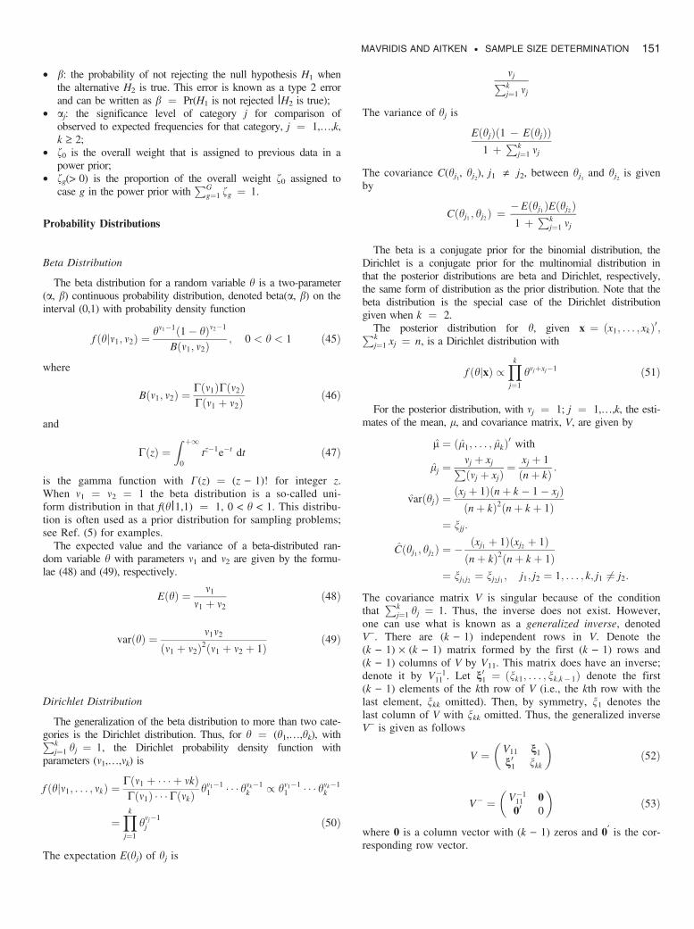
• b: the probability of not rejecting the null hypothesis H1 whenthe alternative H2 is true. This error is known as a type 2 errorand can be written as b ¼ Pr(H1 is not rejected |H2 is true);

• aj: the significance level of category j for comparison ofobserved to expected frequencies for that category, j ¼ 1,…,k,k ‡ 2;

• f0 is the overall weight that is assigned to previous data in apower prior;

• fg(> 0) is the proportion of the overall weight f0 assigned tocase g in the power prior with

PGg¼1 fg ¼ 1.

Probability Distributions

Beta Distribution

The beta distribution for a random variable h is a two-parameter(a, b) continuous probability distribution, denoted beta(a, b) on theinterval (0,1) with probability density function

f ðhjm1; m2Þ ¼hm1�1ð1� hÞm2�1

Bðm1; m2Þ; 0 < h < 1 ð45Þ

where

Bðm1; m2Þ ¼Cðm1ÞCðm2ÞCðm1 þ m2Þ

ð46Þ

and

CðzÞ ¼Z þ1

0tz�1e�t dt ð47Þ

is the gamma function with C(z) ¼ (z ) 1)! for integer z.When m1 ¼ m2 ¼ 1 the beta distribution is a so-called uni-form distribution in that f(h|1,1) ¼ 1, 0 < h < 1. This distribu-tion is often used as a prior distribution for sampling problems;see Ref. (5) for examples.

The expected value and the variance of a beta-distributed ran-dom variable h with parameters m1 and m2 are given by the formu-lae (48) and (49), respectively.

EðhÞ ¼ m1

m1 þ m2ð48Þ

varðhÞ ¼ m1m2

ðm1 þ m2Þ2ðm1 þ m2 þ 1Þð49Þ

Dirichlet Distribution

The generalization of the beta distribution to more than two cate-gories is the Dirichlet distribution. Thus, for h ¼ (h1,…,hk), withPk

j¼1 hj ¼ 1, the Dirichlet probability density function withparameters (m1,…,mk) is

f ðhjm1; . . . ; mkÞ ¼Cðm1 þ � � � þ mkÞCðm1Þ � � �CðmkÞ

hm1�11 � � � hmk�1

k / hm1�11 � � � hmk�1

k

¼Yk

j¼1

hmj�1j ð50Þ

The expectation E(hj) of hj is

mjPkj¼1 mj

The variance of hj is

EðhjÞð1 � EðhjÞÞ1 þ

Pkj¼1 mj

The covariance C(hj1, hj2

), j1 „ j2, between hj1and hj2

is givenby

Cðhj1 ; hj2Þ ¼�Eðhj1ÞEðhj2Þ1 þ

Pkj¼1 mj

The beta is a conjugate prior for the binomial distribution, theDirichlet is a conjugate prior for the multinomial distribution inthat the posterior distributions are beta and Dirichlet, respectively,the same form of distribution as the prior distribution. Note that thebeta distribution is the special case of the Dirichlet distributiongiven when k ¼ 2.

The posterior distribution for h, given x ¼ ðx1; . . . ; xkÞ0;Pkj¼1 xj ¼ n, is a Dirichlet distribution with

f ðhjxÞ /Yk

j¼1

hmjþxj�1 ð51Þ

For the posterior distribution, with mj ¼ 1; j ¼ 1,…,k, the esti-mates of the mean, l, and covariance matrix, V, are given by

l ¼ ðl1; . . . ; lkÞ0 with

lj ¼mj þ xjPðmj þ xjÞ

¼ xj þ 1ðnþ kÞ :

varðhjÞ ¼ðxj þ 1Þðnþ k � 1� xjÞðnþ kÞ2ðnþ k þ 1Þ

¼ njj:

Cðhj1 ; hj2Þ ¼ �ðxj1 þ 1Þðxj2 þ 1Þðnþ kÞ2ðnþ k þ 1Þ

¼ nj1j2 ¼ nj2j1 ; j1; j2 ¼ 1; . . . ; k; j1 6¼ j2:

The covariance matrix V is singular because of the conditionthat

Pkj¼1 hj ¼ 1. Thus, the inverse does not exist. However,

one can use what is known as a generalized inverse, denotedV). There are (k ) 1) independent rows in V. Denote the(k ) 1) · (k ) 1) matrix formed by the first (k ) 1) rows and(k ) 1) columns of V by V11. This matrix does have an inverse;denote it by V�1

11 . Let n01 ¼ ðnk1; . . . ; nk;k� 1Þ denote the first(k ) 1) elements of the kth row of V (i.e., the kth row with thelast element, nkk omitted). Then, by symmetry, n1 denotes thelast column of V with nkk omitted. Thus, the generalized inverseV) is given as follows

V ¼ V11 n1n01 nkk

� �ð52Þ

V� ¼ V�111 000 0

� �ð53Þ

where 0 is a column vector with (k ) 1) zeros and 0¢ is the cor-responding row vector.


sample size determination for categorical responsescgga/jfs2009mavridis.pdf · sample size...

Documents