biometrical modeling of twin and family data · biometrical modeling of twin and family data sophia...

Biometrical modeling of twin and family data

Sophia Rabe-HeskethGraduate School of Education & Graduate Group in Biostatistics

University of California, BerkeleyInstitute of Education, University of London

joint work with Anders Skrondal and Håkon Gjessing

German Stata Users Group MeetingBerlin, June 2010

– p.1

Outline

Genetic variance components model: ACDE

Liability model for binary traits

Models for twin designs

Assumptions and two parameterizations (P1, P2) asmixed/multilevel models

Continuous adult height: P1 ACE, P2 ACE

Continuous neuroticism: P2 ADE

Binary hay-fever status: P2 ADE & AE

Models for nuclear family designs

Continuous birth weight data

– p.2

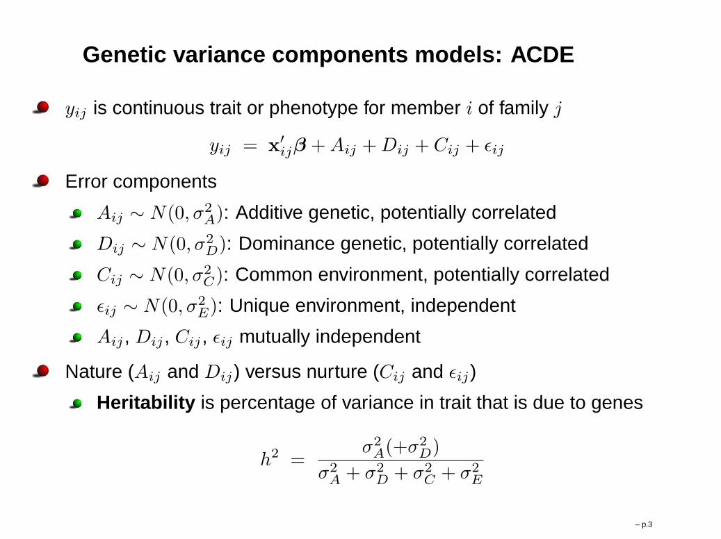
Genetic variance components models: ACDE

yij is continuous trait or phenotype for member i of family j

yij = x′

ijβ +Aij +Dij + Cij + εij

Error components

Aij ∼ N(0, σ2A): Additive genetic, potentially correlated

Dij ∼ N(0, σ2D): Dominance genetic, potentially correlated

Cij ∼ N(0, σ2C): Common environment, potentially correlated

εij ∼ N(0, σ2E): Unique environment, independent

Aij , Dij , Cij , εij mutually independent

Nature (Aij and Dij) versus nurture (Cij and εij)

Heritability is percentage of variance in trait that is due to genes

h2 =σ2A(+σ2

D)

σ2A + σ2

D + σ2C + σ2

E

– p.3

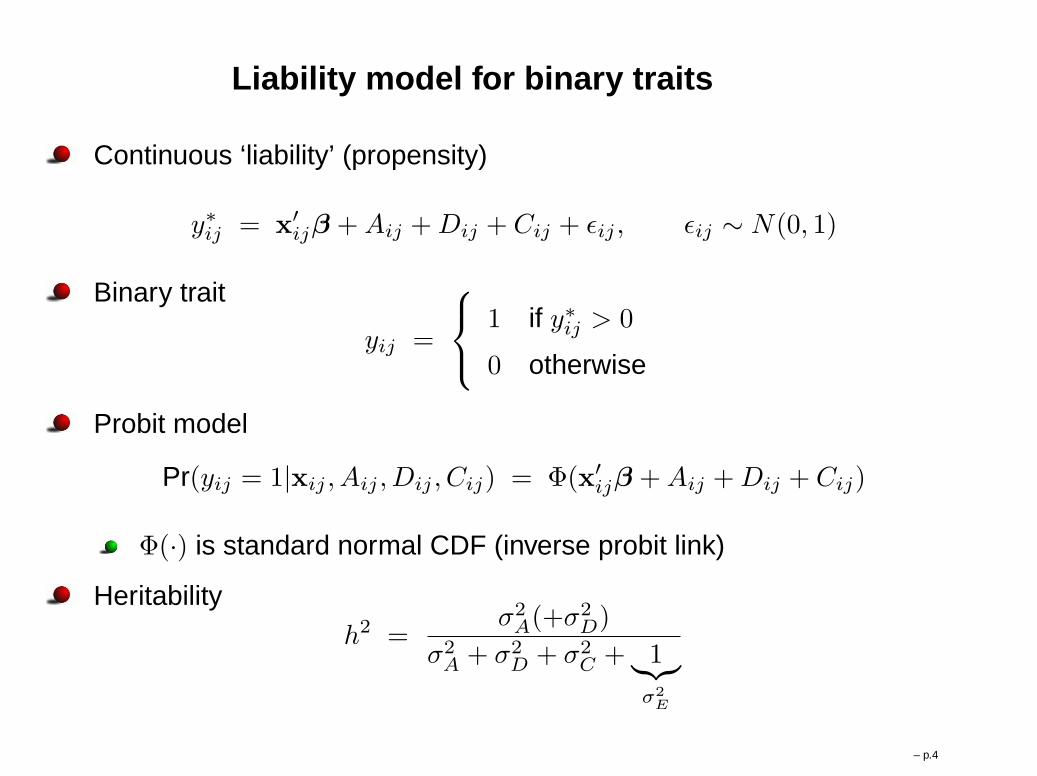
Liability model for binary traits

Continuous ‘liability’ (propensity)

y∗ij = x′

ijβ +Aij +Dij + Cij + εij , εij ∼ N(0, 1)

Binary trait

yij =

1 if y∗ij > 0

0 otherwise

Probit model

Pr(yij = 1|xij , Aij , Dij , Cij) = Φ(x′

ijβ +Aij +Dij + Cij)

Φ(·) is standard normal CDF (inverse probit link)

Heritabilityh2 =

σ2A(+σ2

D)

σ2A + σ2

D + σ2C + 1︸︷︷︸

σ2

E

– p.4

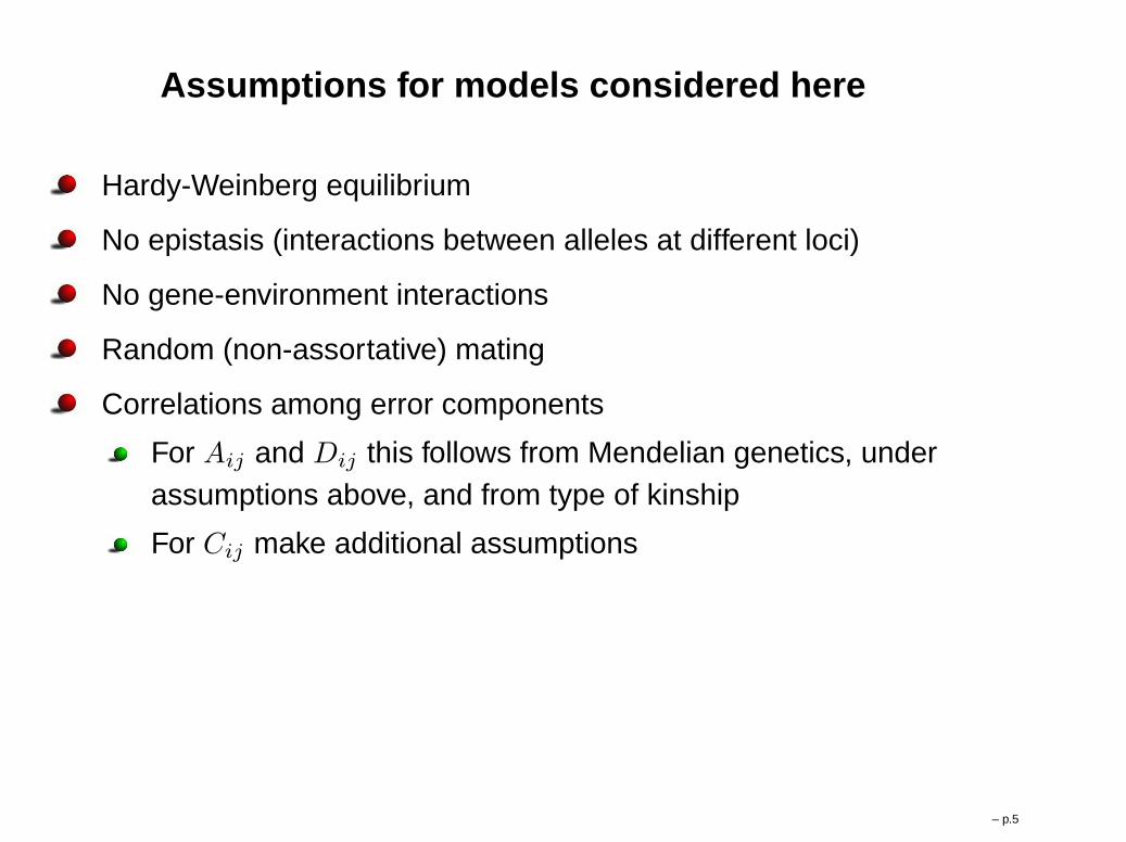
Assumptions for models considered here

Hardy-Weinberg equilibrium

No epistasis (interactions between alleles at different loci)

No gene-environment interactions

Random (non-assortative) mating

Correlations among error components

For Aij and Dij this follows from Mendelian genetics, underassumptions above, and from type of kinship

For Cij make additional assumptions

– p.5

Model formulation

Usually biometrical models for twin and family data expressed as amulti-group structural equation models (SEMs) and fitted in Mx,Mplus, or other SEM software

Can formulate models as mixed/multilevel models [Rabe-Hesketh,

Gjessing & Skrondal, 2008] and fit them in Stata

xtmixed : Continuous phenotypes and models that do notrequire equality constraints for variances at different levels

gllamm : Continuous, binary (or ordinal) phenotypes

Models with the fewest random effects are easiest to estimate forbinary (or ordinal) phenotypes

– p.6

Models for twin designs

Monozygotic (MZ) or ‘identical’ twins share all genes by descent

Dizygotic (DZ) or ‘fraternal’ twins share half their genes by descent

Equal environment assumption: MZ and DZ twins have same degreeof similarity in their environments, so that excess similarity betweenMZ twins can be attributed to the greater proportion of shared genes

– p.7

Models for twin designs (cont’d)

Consider two twin pairs: (MZ1, MZ2), (DZ1, DZ2):

Cov(A) = σ2A

1 1 0 0

1 1 0 0

0 0 1 1/2

0 0 1/2 1

Cov(D) = σ2D

1 1 0 0

1 1 0 0

0 0 1 1/4

0 0 1/4 1

Cov(C) = σ2C

1 1 0 0

1 1 0 0

0 0 1 1

0 0 1 1

Cov(E) = σ2E

1 0 0 0

0 1 0 0

0 0 1 0

0 0 0 1

ACDE model not identified here; consider ACE and ADE (as well asAE, CE)

– p.8

Twin datasets

All data: Mis dummy for MZ; pair is twin-pair j; member is i

Continuous adult heights twin_bmi.dta [Posthuma & Boomsma, 2005]

Variables height (in cm) and male

304 twin pairs (13% with height missing for one member)307 DZ members (40% male). 262 MZ members (43% male)

Continuous neuroticism twin_neur.dta [Sham, 1998]

Variable neurot (Eysenck personality questionnaire)

794 female twin pairs (no missing data)272 DZ pairs. 522 MZ pairs

Binary hay fever status twin_hay.dta [Hopper et al., 1990]

Variables h, male , pair-level frequency weights freq

3,807 twin pairs (no missing data)2,009 DZ pairs (18% male, 45% mix). 1,798 MZ pairs (31% male)

– p.9

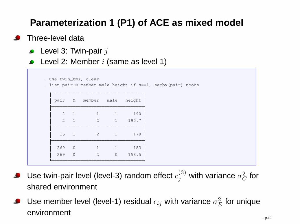
Parameterization 1 (P1) of ACE as mixed model

Three-level data

Level 3: Twin-pair jLevel 2: Member i (same as level 1)

. use twin_bmi, clear

. list pair M member male height if s==1, sepby(pair) noobs

pair M member male height

2 1 1 1 190

2 1 2 1 190.7

16 1 2 1 178

269 0 1 1 183

269 0 2 0 158.5

Use twin-pair level (level-3) random effect c(3)j with variance σ2C for

shared environment

Use member level (level-1) residual εij with variance σ2E for unique

environment– p.10

Parameterization 1 (P1) of ACE as mixed model (cont’d)

Problem: Additive genetic component completely shared (correlation1) for MZ twins and partially shared (correlation 0.5) for DZ twins

Solution:

Shared component a(3)j with variance σ2A contributes only half as

much variance to DZ twins as to MZ twins

a(3)j [Mj +

√1

2M j ]

Mj is dummy for MZM j = 1−Mj is dummy for DZ

Remaining variance for DZ twins comes from unsharedcomponent a(2)ij with variance σ2

A

a(2)ij

√1

2M j

– p.11

Continuous adult height: P1 ACE

Cannot estimate in xtmixed because of equality constraint forvariances at different levels

In gllamm :

generate var3 = M + sqrt(1/2) * (1-M)

generate var2 = sqrt(1/2) * (1-M)

eq var3: var3

eq var2: var2

generate one = 1

eq cons: one

cons def 1 [mem1_1]var2 = [pai2_1]var3

gllamm height male, i(member pair) nrf(1 2)

eqs(var2 var3 cons) nocor constr(1) adapt

– p.12

Continuous adult height: P1 ACE (cont’d)

log likelihood = -1727.820312522015

( 1) [mem1_1]var2 - [pai2_1]var3 = 0

height Coef. Std. Err. z P>|z| [95% Conf. Interval]

male 12.99536 .6166593 21.07 0.000 11.78673 14.20398

_cons 167.9549 .438026 383.44 0.000 167.0963 168.8134

Variance at level 1

--------------------------------------------------- ---------------------------

2.392252 (.30445676)

Variances and covariances of random effects

--------------------------------------------------- ---------------------------

*** level 2 (member)

var(1): 40.342974 (5.1760754)

*** level 3 (pair)

var(1): 40.342974 (5.1760754)

cov(2,1): fixed at 0

var(2): 1.8175006 (5.2567317)

--------------------------------------------------- ---------------------------

. disp 40.342974/(40.342974+1.8175006+ 2.392252 )

.90551078

– p.13

Parameterization 2 (P2) of ACE as mixed model

Three-level model

Level 3: Twin-pair j

Level 2: Hybrid k, k =

pair j for MZ twins

member i for DZ twins

Level 1: Member i

εij with variance σ2E for unique environment as before

u(2)kj with variance σ2

A/2 for half the additive genetic variance that isshared for MZ and unique for DZ

u(3)j with variance σ2

A/2 + σ2C for the other half of additive genetic

variance that is shared for everyone and for common environment

Note: Only two random effects instead of three

– p.14

Continuous adult height: P2 ACE

generate k = pair if M==1

replace k = member if M==0

xtmixed height male || pair: || k:, mle variance

Wald chi2(1) = 446.47

Log likelihood = -1727.8203 Prob > chi2 = 0.0000


male 12.99535 .6150212 21.13 0.000 11.78993 14.20077

_cons 167.9549 .4379076 383.54 0.000 167.0966 168.8131

Random-effects Parameters Estimate Std. Err. [95% Conf. Interval]

pair: Identity

var(_cons) 21.98932 3.482324 16.12173 29.99244

k: Identity

var(_cons) 20.17123 2.588088 15.68621 25.9386

var(Residual) 2.392253 .3044573 1.864131 3.069997

– p.15

Continuous adult height: P2 ACE: (cont’d)

Already have σ̂2E

Get σ̂2A and σ̂2

C using nlcom

. nlcom (var_A: 2 * exp(2 * [lns2_1_1]_cons))

> (var_C: exp(2 * [lns1_1_1]_cons)-exp(2 * [lns2_1_1]_cons))

var_A: 2 * exp(2 * [lns2_1_1]_cons)

var_C: exp(2 * [lns1_1_1]_cons)-exp(2 * [lns2_1_1]_cons)


var_A 40.34246 5.176177 7.79 0.000 30.19734 50.48758

var_C 1.818089 5.256801 0.35 0.729 -8.485051 12.12123

* Heritability:

. disp 40.34246/(40.34246+1.818089+2.392253)

.90549771

Use _diparm with option ci(probit) to get confidence interval forheritability; however, requires derivatives

Would be nice to have ci(probit) option in nlcom !– p.16

Parameterization 2 for ACE, AE, ADE, CE

ACE: σ̂2A = 2V̂ar(u(2)

kj ) and σ̂2C = V̂ar(u(3)

k )− V̂ar(u(2)kj )

Potential problem: σ̂2C can be negative

Solution 1: AE: constrain σ2C to zero by constraining

Var(u(3)j ) = Var(u(2)

kj ) (in gllamm only; see slide 22)

Solution 2: ADE (see below)

ADE (same model as ACE):

σ̂2A = 3V̂ar(u(3)

j )− V̂ar(u(2)kj ) and σ̂2

D = 2[V̂ar(u(2)kj )− V̂ar(u(3)

j )]

CE: Set Var(u(2)kj ) = 0, giving two-level model

Note: Conventional likelihood ratio tests to compare models areconservative [Dominicus et al., 2006]

– p.17

Continuous neuroticism: P2 ADE

generate k = pair if M==1

replace k = member if M==0

xtmixed neurot || pair: || k:, mle variance

neurot Coef. Std. Err. z P>|z| [95% Conf. Interval]

_cons 10.23203 .1237788 82.66 0.000 9.989426 10.47463


pair: Identity

var(_cons) 3.345268 1.034871 1.824351 6.134134

k: Identity

var(_cons) 5.023933 1.187507 3.161151 7.984402

var(Residual) 9.559881 .5823694 8.483966 10.77224

– p.18

Continuous neuroticism: P2 ADE (cont’d)

Note that σ̂2C = V̂ar(u(3)

k )− V̂ar(u(2)kj ) < 0

For ADE model, get σ̂2A and σ̂2

D using nlcom

. nlcom (var_A: 3 * exp(2 * [lns1_1_1]_cons) - exp(2 * [lns2_1_1]_cons) )

> (var_D: 2 * (exp(2 * [lns2_1_1]_cons) - exp(2 * [lns1_1_1]_cons)))

var_A: 3 * exp(2 * [lns1_1_1]_cons) - exp(2 * [lns2_1_1]_cons)

var_D: 2 * (exp(2 * [lns2_1_1]_cons) - exp(2 * [lns1_1_1]_cons))

neurot Coef. Std. Err. z P>|z| [95% Conf. Interval]

var_A 5.01187 4.088337 1.23 0.220 -3.001123 13.02486

var_D 3.357331 4.180764 0.80 0.422 -4.836817 11.55148

* heritability

. disp (5.01187+3.357331)/(5.01187+3.357331+9.559881)

.46679473

– p.19

Binary hay fever status: P2 ADE

generate num3 = freq

gllamm h male, i(k pair) link(probit) fam(binom)

adapt weight(num)

log likelihood = -4603.3053

h Coef. Std. Err. z P>|z| [95% Conf. Interval]

male -.1636205 .0534943 -3.06 0.002 -.2684675 -.0587736

_cons -.6874611 .040749 -16.87 0.000 -.7673276 -.6075945


--------------------------------------------------- ---------------------------

*** level 2 (k)

var(1): .89076163 (.16434027)

*** level 3 (pair)

var(1): .65503535 (.10341492)

--------------------------------------------------- ---------------------------

Note: Estimation fast because only 40 rows of data andpair-level frequency weights

– p.20

Binary hay fever status: P2 ADE (cont’d)

. nlcom (var_A: 3 * [pair2]_consˆ2 - [k1]_consˆ2)

> (var_D: 2 * ([k1]_consˆ2 - [pair2]_consˆ2))

var_A: 3 * [pair2]_consˆ2 - [k1]_consˆ2

var_D: 2 * ([k1]_consˆ2 - [pair2]_consˆ2)


var_A 1.074344 .3679161 2.92 0.003 .3532421 1.795447

var_D .4714526 .4085908 1.15 0.249 -.3293708 1.272276

. * Heritability

. disp (1.074344+.4714526)/(1.074344+.4714526+1)

.60719564

– p.21

Binary hay fever status: P2 AE (cont’d)

constr def 1 [pair2]_cons = [k1]_cons

gllamm h male, i(k pair) link(probit) fam(binom) adapt

weight(num) constr(1)

log likelihood = -4604.027077892745

( 1) - [k1]_cons + [pair2]_cons = 0


male -.1608356 .0523616 -3.07 0.002 -.2634623 -.0582088

_cons -.6758232 .0388389 -17.40 0.000 -.751946 -.5997004


--------------------------------------------------- ---------------------------

*** level 2 (k)

var(1): .73240456 (.08174648)

*** level 3 (pair)

var(1): .73240456 (.08174648)

--------------------------------------------------- ---------------------------

. disp .73240456/(.73240456+1)

.42276762

– p.22

ACE for nuclear family designs

Nuclear family with two children (mother, father, child1, child2)

Cov(A) = σ2A

1 0 1/2 1/2

0 1 1/2 1/2

1/2 1/2 1 1/2

1/2 1/2 1/2 1

Cov(C) = σ2C

1 0 0 0

0 1 0 0

0 0 1 1

0 0 1 1

Cov(E) = σ2E

1 0 0 0

0 1 0 0

0 0 1 0

0 0 0 1

– p.23

Parametrization as mixed model

Four-level model

Level 4: Family k

Level 3: Hybrid: Sibling pair j, individual parents i

Level 2: Member i (same as level 1)

yijk = x′

ikβ+a(4)1k [Mi+Ki/2]+a

(4)2k [Fi+Ki/2]+a

(2)ijk[Ki/

√2]+c

(3)jk +εijk

Mi is a dummy for mother, Fi for father, Ki for child

Var(c(3)jk ) = σ2C and Var(εijk) = σ2

E

First three terms represent additive genetic component withVar(a(4)1k ) = Var(a(4)2k ) = Var(a(2)ijk) = σ2

A

a(4)1k and a

(4)2k induce the required additive genetic covariances

between each parent and each child and among the children

a(2)ijk provides remaining variance σ2

A/2 for children

– p.24

Continuous birthweight: Nuclear family data

1000 Nuclear families from Norwegian birth registry [Magnus et al., 2001]

One child per family (no level 3, j), model simplifies to two-levelmodel

yijk = x′

ikβ + a(4)1k [Mi+Ki/2] + a

(4)2k [Fi+Ki/2] + a

(2)ijk[Ki/

√2] + c

(3)jk + εijk

yik = x′

ikβ + a(4)1k [Mi+Ki/2] + a

(4)2k [Fi+Ki/2] + a

(4)3k [Ki/

√2] + εij

Model with c(3)jk not identified

a(2)ijk[Ki/

√2] ≡ a

(4)3k [Ki/

√2] because Ki is non-zero for one

member per family

Level 4 becomes level 2

yik = x′

ikβ+a(2)1k [Mi+Ki/2]+a

(2)2k [Fi+Ki/2]+a

(2)3k [Ki/

√2]+ εij

– p.25

Continuous birthweight: Nuclear family data (cont’d)

fam_birthwt.dta contains M, F, K, family , bwt and

male : dummy for being malefirst : dummy for being the first childmidage : dummy for mother aged 20-35 at time of birthhighage : dummy for mother’s age above 35 at time of birthbirthyr : year of birth minus 1967

. list family M F K male birthyr bwt if family<3, sepby(family ) noobs

family M F K male birthyr bwt

1 1 0 0 0 5 3520

1 0 1 0 1 6 3940

1 0 0 1 0 26 3240

2 1 0 0 0 5 3660

2 0 1 0 1 2 3990

2 0 0 1 1 29 4330

– p.26

Estimation using xtmixed

Stata commands:

generate var1 = M + K/2

generate var2 = F + K/2

generate var3 = K/sqrt(2)

xtmixed bwt male first midage highage birthyr

|| family: var1 var2 var3,

nocons cov(ident) mle variance

Note: Option covariance(identity) enforces variance equalityconstraint (and independence of error components) within a level

– p.27

Estimation using xtmixed

. xtmixed bwt male first midage highage birthyr || family: va r1 var2 var3,

> nocons cov(ident) mle variance

bwt Coef. Std. Err. z P>|z| [95% Conf. Interval]

male 158.4546 17.34853 9.13 0.000 124.4521 192.4571

first -139.3974 18.7415 -7.44 0.000 -176.13 -102.6647

midage 57.0553 31.89569 1.79 0.074 -5.459111 119.5697

highage 118.8564 54.67221 2.17 0.030 11.70082 226.0119

birthyr 3.627799 .6882291 5.27 0.000 2.278894 4.976703

_cons 3461.459 34.77956 99.53 0.000 3393.292 3529.625


family: Identity

var(var1 var2 var3) 99263.68 10157.96 81223.99 121310

var(Residual) 133560.1 9069.929 116915.7 152574.2

LR test vs. linear regression: chibar2(01) = 97.80 Prob >= ch ibar2 = 0.0000

– p.28

Concluding remarks

Advantage of using multilevel models

More widely known and available in software than SEM

Can handle varying family sizes and missing data easily

Can extend to more levels, e.g., random neighborhoodenvironment effects

Other models considered in [Rabe-Hesketh, Skrondal & Gjessing, 2008]

Sibling and cousin data

Prameterization 1 for Twin ADE models

Wishlist for Stata 12

Constraints for variance-covariance parameters in xtmixed ,particularly equality constraints across levels

nlcom with ci(probit) option

– p.29

References to own work

Rabe-Hesketh, S., Skrondal, A. and Gjessing, H. K. (2008).Biometrical modeling of twin and family data using standard softwarefor mixed models. Biometrics 64, 280-288.

Rabe-Hesketh, S. and Skrondal, A. (2008). Multilevel andLongitudinal Modeling Using Stata (Second Edition). StataPress.

Rabe-Hesketh, S., Skrondal. A. and Pickles, A. (2005). Maximumlikelihood estimation of limited and discrete dependent variablemodels with nested random effects. Journal of Econometrics 128,301-323.

– p.30

Other references

Dominicus, A., Skrondal, A., Gjessing, H. K., Pedersen, N. andPalmgren, J. (2006). Likelihood ratio tests in behavioral genetics:Problems and solutions. Behavior Genetics 36, 331-340.

Hopper, J. L., Hannah, M. C. and Mathews, J. D. (1990). Twinconcordance for a binary trait: III. A binary analysis of hay fever andasthma. Genetic Epidemiology 7, 277-289.

Magnus, P., Gjessing, H. K., Skrondal, A. and Skjærven, R. (2001).Paternal contribution to birth weight. Journal of Epidemiology andCommunity Health 55, 873-877.

Posthuma, D. and Boomsma, D. I. (2005). Mx Scripts library:Structural equation modeling scripts for twin and family data.Behavior Genetics 35, 499-505.

Sham, P. (1998). Statistics in Human Genetics. London: Arnold.

– p.31

biometrical modeling of twin and family data · biometrical modeling of twin and family data sophia...

Documents