biomechanics of rowing biomechanics in nolte.pdf · length usually occurs at stroke rate around 24...

◾ 105

Chapter 9

Biomechanics of Rowing

Valery Kleshnev

Performance in rowing is a complex matter, as is performance in any sport. It requires high physiological power production, effective technique, strong psychology, and

smart race strategy. The main purpose of biomechanics in rowing is improvement of technique. Previous authors have presented charts of rowing biomechanics based on mechanical relationships between variables (Affeld, Schichl, & Ziemann, 1993; Kleshnev, 2007). Because this book is intended mainly for coaches and rowers, we have organized the general picture by the components of rower’s technical skills that can be analyzed to develop good technique and the biomechanical variables that need to be measured to provide data for the analysis. Figure 9.1 on page ___ shows relationships among these components and variables. Obviously, the real picture is much more complicated since the components of rowing technique are interrelated and usually affected by more than one biomechanical variable. For example, rowing style is related to many other components of technique, including blade and boat efficiencies, force curve, drive length, and others. Therefore, we can consider rowing style to be the key component of rowing technique.

The chart of rowing biomechanics has three levels: measurement, analysis, and per-formance. At the measurement level we collect information from sensors, process it (e.g., apply calibration and filters), store it, and feed it into the next analysis level.

During analysis, we combine information from various channels, calculate derivative variables and values, and produce meaningful knowledge out of them. There are two separate areas at the analysis level: theory and practice. In the theory area, we analyze acquired data with the purpose of producing and publishing common knowledge (e.g., average values in athlete groups, correlations, normative criteria). In the practice area, we compare the acquired data with the normative criteria and produce conclusions and recommendations for a specific athlete that are fed into the next performance level.

At the performance level, we try to correct rowing technique with instructions obtained at the analysis level. Various methods of feedback can be used at this level, including delayed, postexercise, and immediate feedback. Parameters of rowing technique need

106 ◾ Kleshnev

to be measured and analyzed again after correction, which creates an endless loop of technique improvement.

In this chapter, we will discuss components of rowing biomechanics according to the direction of information flow: from measurement to analysis and then to performance.

Biomechanical measuRementAny science starts with obtaining quantitative information and analyzing it. Rowing is a productive sport in terms of biomechanical measurements. There are many points where transducers can be mounted, including the oar, gate, pin, stretcher, and seat. Therefore, biomechanical measurement in rowing can be a sophisticated process. Here we describe only those variables that we measure in standard biomechanical testing and use for analysis and technique improvement. Many other variables could be measured for research purposes.

horizontal Oar angle and Drive LengthHorizontal oar angle is a key variable in rowing biomechanics because it is used for defining the drive and recovery phases of the stroke cycle. We assume the horizontal angle to be 0 at the perpendicular position of the oar axis relative to the longitudinal boat axis. The beginning of the stroke cycle occurs when the oar passes 0° horizontal angle during recovery.

The horizontal angle can be measured at the oar (figure 9.2, a-b) or at the gate. The last method produces 4° to 5° larger numbers, which occur mainly by means of release angles. Two reasons for this phenomenon can be speculated:

1. Bend of the oar shaft. When force increases at the first half of the drive, angular velocity of the oar is slightly higher. At the second half of the drive, the oar extends, and its rotation appears to be slower than the gate rotation. Oar bend probably is the reason for small differences in catch angle and has no effect on finish angle because the force at this point is minor.

E5068/Nolte/Rowing Faster, 2e/F09.01/404119/TimB/R1

Result

Horizontal oarangles

Segments’velocities

Boat velocityand acceleration

Verticaloar angle

Technique(biomechanics)

Metabolic power(physiology)

Race strategyPsychology

EfficiencyEffectiveness

Rowingpower

Forcecurve

Rowing style andrower’s efficiency

Boatefficiency

Bladeefficiency

Performance level

Analysis level

Measurementlevel

Handle andgate force

Figure 9.1 Simplified chart of rowing biomechanics in relation to performance.

Biomechanics of Rowing ◾ 107

2. Backlash of the oar sleeve in the gate. This is probably the main contributor to the differences in angle readings. It depends on the geometry of the gate, sleeve, and button, plus coordination of feathering along with horizontal and vertical movements of the oar. It is difficult to predict the amount of backlash that varies with rowers’ release motions.

Catch angle αcatch is defined as the minimal negative oar angle and finish angle αfin as the maximal positive oar angle. Total rowing angle αtot is calculated as the difference between finish and catch angles:

αtot = αfin − αcatch.

Drive length is defined as the displacement of the center of the handle from catch to finish and can be calculated using actual inboard length Linb-a measured from the center of the pin to the middle of the handle (6 cm from the handle top in sculling and 15 cm in rowing):

Larc = Linb-a × π × αtot / 180.

The drive length is a critical component of rowing effectiveness (Nolte, 1991). The maximal length usually occurs at stroke rate around 24 spm. The length is 2 to 3 cm shorter at low rates and much shorter at high rates. Reduction of the stroke length is more significant in bigger boats. Measurements show that in 4x and 8+ boats, it can be up to 10 to 11 cm shorter at 40 spm relative to 24 spm, but in smaller boats it is only 6 to 7 cm shorter at the same rate. Shortening of the stroke length at higher rates occurs at both ends of the stroke: catch and finish. At catch it is more significant in sweep boats (6-10 cm between 24 and 40 spm) than in sculling (4-6 cm). At finish the shortening is noticeable in sculling (4-6 cm) but very small in sweep boats. Therefore, decreased the stroke length at higher ratings occurs mainly at catch in sweep boats and at both ends in sculling.

Force MeasurementsForce applied by the rower is the earliest measurement ever taken in rowing biomechan-ics—it was measured in 1896 by Atkinson (Filter, 2009). Similar to oar angle, the force can be measured at the oar handle or at the gate or pin (figure 9.3).

E5068/Nolte/Rowing Faster, 2e/F09.02a/404120/TimB/R1

RecoveryHor

izon

tal a

ngle

(°)

Drive

Oar Gate

Recovery

6040200

–20–40–60

Drive Release

Ang

ular

vel

ocity

(ra

d/s) 3

2

1

0

–1

–2

Oar flexion

Oarextension

Backlash of theoar in the gate

Figure 9.2 (a) Horizontal angle α measured at the oar and gate; (b) device for measurement of horizontal and vertical oar angles.

a b

108 ◾ Kleshnev

These methods have the following features:

1. Handle force Fhnd can be measured perpendicular to the oar direction either with strain gauges applied directly on the oar shaft or with detachable sensors. In fact, the sensor measures the oar bend, which is proportional to the torque M or moment of the force Fhnd and can be calibrated as a force applied at a known point on the handle. The rower’s power production P can be derived as

P = M × ω = Fhnd × Lin-a × ω,

where Lin-a is the actual oar inboard lever and ω is oar angular velocity, which can be derived from measurements of the horizontal oar angle. In this case the calculated power is not affected by the point of the rower’s force application, which is unknown and may vary significantly, especially in sweep rowing. With an estimated error of 1%, this is the most accurate method for measurement of rower’s power. The practical problem of this method is the necessity to calibrate every oar, which can be solved with modern technology (Caplan & Gardner, 2007).

The resultant force Fhnd-res, which the rower applies to the handle, is not always per-pendicular to the oar axis. Therefore, it can be resolved into the perpendicular Fhnd and axial Fhnd-ax components. The last is quite difficult to measure, but it does not produce any mechanical power at the oar. It is statically transferred through the oar shaft and creates axial force at the gate Fgate-ax, which is a sum of vectors Fhnd-ax and axial force at the blade Fbl-ax. Then, the axial force Fgate-ax is transferred through the gate, pin, and rigger and statically balanced with the stretcher force Fstr. Therefore, a rower should apply only a small axial force to keep the button in contact with the gate and pull the handle as close to perpendicular as possible.

The perpendicular component of the blade force Fbl can be measured using the same method as was described previously for the handle force. This would produce the same accuracy of the rower’s power calculation.

2. The gate rotates together with the oar, and the perpendicular Fgate and axial Fgate-ax components of the gate force can be measured in the reference frame of the oar using various instrumented gates. Rower’s power can be derived using equation on page ___, but Fhnd must be calculated as

Fhnd = Fgate × [Lout-a / (Lin-a + Lout-a)],

where Lout-a is actual outboard length from pin to the center of the blade force. We do not know Lin-a and Lout-a exactly because actual points of force application during rowing are uncertain. We can only guess that they are located at the center of the handle and

E5068/Nolte/Rowing Faster, 2e/F09.03/404122/TimB/R1

Lin-a

Fhnd-ax

Fhnd-res

Fstr

FpinY

FgateFg-p-res

Vboat

Fpin

ααβ

Fgate-axFhnd

Fbl-ax

FblFbl-res

Lout-a

Figure 9.3 Schematics of force measurement in rowing.


blade. The estimated error of rower’s power calculation using this method could be up to 5%. The sum of the normal Fgate and axial Fgate-ax components is a resultant gate force Fg-p-res, which is transferred to the pin.

3. The pin is fixed relative to the boat and the pin sensor measures force in the reference frame of the boat (Hill & Fahrig, 2009). Usually it measures only parallel to the boat axis component Fpin of the resultant gate-pin force Fg-p-res. Rower’s power can be derived using the first and second equations (pages ___ and ___); however, gate force Fgate must be derived as

Fgate = Fpin × cos α.

Only part of the rower’s force production can be measured using this method (e.g., only half at the catch oar angle, -60° as cos[60o] = 0.5). Also, the readings are affected by axial gate force Fgate-ax, which, as we have shown, does not produce power. The estimated error of the rower’s power calculation is 10% in sculling and up to 20% in rowing. Accuracy of this method can be improved with two-dimensional sensors of pin force, which can also measure perpendicular to the boat component FpinY. In this case, the accuracy would match the gate force sensors. The magnitude of the resultant force Fg-p-res is determined as

Fg-p-res = (Fpin2 + FpinY2)0.5.

Its direction can be defined by the angle β:

β = accros(Fpin / Fg-p-res)

Then perpendicular component Fgate is derived using known gate angle α.

Fgate = Fg-p-res × cos(α − β).

The situation with accuracy is the opposite if the purpose is calculation of balance of forces on the hull, which could be a target in some research studies. Usually, the stretcher force Fstr is measured in these studies and propulsive force acting on the boat Fprop-boat can be derived for each rower:

Fprop-boat = Fpin − Fstr.

If the force is measured at the handle, then Fgate must be derived from Fhnd using Lin-a and Lout-a and then Fpin obtained using oar angle α. In this case, measurement of the pin force Fpin is the most accurate method, and its calculation from measurement of Fhnd can give a significant error, especially in sweep rowing.

Segment VelocitiesThe position of the sliding seat can be measured using a spring-loaded transducer with a string. Similarly, position of the top of the trunk can be measured with the same trans-ducer mounted on a mast at the level of the sternoclavicular joint (figure 9.4a).

Strictly speaking, displacement of legs should be defined at the hip joint, the center of which is located 8 to 10 cm above the seat. However, from a practical standpoint it is much more convenient to measure seat displacement.

Velocities can be derived by differentiating the displacement data:

◾ Leg velocity is derived from the seat displacement.

◾ Trunk velocity is derived as the difference between top-of-the-trunk and seat displacements.

110 ◾ Kleshnev

◾ Arm velocity is derived as the difference between top-of-the-trunk and handle dis-placements. The handle displacement is obtained from oar angle and actual inboard (see the third equation above).

Figure 9.4b shows typical velocity curves of the handle and body segments for a single sculler at a stroke rate of 35 spm and average boat speed of 5 mps (meters per second) measured with the described method.

Boat, rower, and System VelocitiesFor many decades, boat velocity was considered to be the most important variable in rowing biomechanics. Obviously, average boat speed is the resultant parameter directly related with performance. As soon as instantaneous boat velocity became available for measurements, it was used to indicate efficiency of rowing techniques (Zatsiorsky & Yakunin, 1991), and a theory was developed that emphasized smoothness of boat velo-city. This theory had a negative effect on rowing technique, because boat velocity cannot be constant due to two reasons:

1. Periodical application of propulsive force

2. Movement of the heavier mass of the rower relative to the lighter mass of the boat

Later it was found that fluctuations of boat velocity play a relatively small role in per-formance and can be changed very little with rowing technique (Klavora, 1977; Nolte, 1984; Sanderson & Martindale, 1986). The only movement pattern that can improve velocity fluctuations is a smooth movement without jerks at the beginning of the recovery.

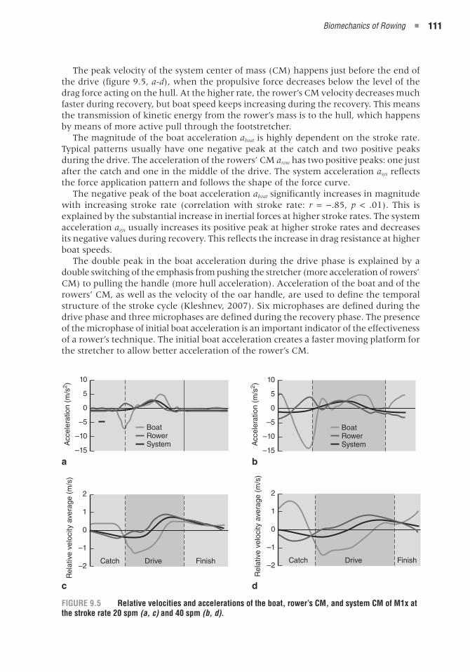
The measure of fluctuations is a variation of the hull speed (ratio of its standard devia-tion to the average). Generally, the variation increases from 11.7% at the rate of 20 spm up to 13.7% at the rate of 40 spm (figure 9.5, c-d). This decreases the efficiency of the boat speed (ratio of actual propulsive power to minimum required power for the same average speed) from 96.25% to 94.79%. This 1.46% difference in efficiency would make the time of a 2,000 m race only 1.5 seconds slower, which is very small compared with the difference in the overall speed: 4.31 mps at 20 spm and 5.29 mps at 40 spm equates to a time difference of 86.1 seconds over 2,000 m.

Seat position sensor

E5086/Nolte/Rowing Faster, 2e/Fig 09.04a/404123/TB/R1

Hip joint

Trunk position sensor

E5068/Nolte/Rowing Faster, 2e/F09.04b/404124/TimB/R1

3

2

1

0–60 –20 10–50 –10 3020

Velocity (m/s)

Angle (°)

DriveCatch

Finish

Handle LegsTrunk Arms

–30–40

–1

–2

–3Recovery

Figure 9.4 (a) Schematics of measurement of the seat and trunk positions; (b) typical graph of the segment and handle velocities.

a b


The peak velocity of the system center of mass (CM) happens just before the end of the drive (figure 9.5, a-d), when the propulsive force decreases below the level of the drag force acting on the hull. At the higher rate, the rower’s CM velocity decreases much faster during recovery, but boat speed keeps increasing during the recovery. This means the transmission of kinetic energy from the rower’s mass is to the hull, which happens by means of more active pull through the footstretcher.

The magnitude of the boat acceleration aboat is highly dependent on the stroke rate. Typical patterns usually have one negative peak at the catch and two positive peaks during the drive. The acceleration of the rowers’ CM arow has two positive peaks: one just after the catch and one in the middle of the drive. The system acceleration asys reflects the force application pattern and follows the shape of the force curve.

The negative peak of the boat acceleration aboat significantly increases in magnitude with increasing stroke rate (correlation with stroke rate: r = −.85, p < .01). This is explained by the substantial increase in inertial forces at higher stroke rates. The system acceleration asys usually increases its positive peak at higher stroke rates and decreases its negative values during recovery. This reflects the increase in drag resistance at higher boat speeds.

The double peak in the boat acceleration during the drive phase is explained by a double switching of the emphasis from pushing the stretcher (more acceleration of rowers’ CM) to pulling the handle (more hull acceleration). Acceleration of the boat and of the rowers’ CM, as well as the velocity of the oar handle, are used to define the temporal structure of the stroke cycle (Kleshnev, 2007). Six microphases are defined during the drive phase and three microphases are defined during the recovery phase. The presence of the microphase of initial boat acceleration is an important indicator of the effectiveness of a rower’s technique. The initial boat acceleration creates a faster moving platform for the stretcher to allow better acceleration of the rower’s CM.


10

5

0

–5

–10

–15

BoatRowerSystemA

ccel

erat

ion

(m/s

2 )


10

5

0

–5

–10

–15

BoatRowerSystemA

ccel

erat

ion

(m/s

2 )

E5068/Nolte/Rowing Faster, 2e/F09.05c/404127/TimB/R1

2

1

0

–1

–2DriveCatch Finish

Rel

ativ

e ve

loci

ty a

vera

ge (

m/s

)

E5068/Nolte/Rowing Faster, 2e/F09.05d/404128/TimB/R1

2

1

0

–1

–2DriveCatch Finish

Rel

ativ

e ve

loci

ty a

vera

ge (

m/s

)

Figure 9.5 relative velocities and accelerations of the boat, rower’s CM, and system CM of M1x at the stroke rate 20 spm (a, c) and 40 spm (b, d).

a b

c d

112 ◾ Kleshnev

Vertical Oar angleFor practical reasons we assume 0 vertical angle (θ) of the oar is located at the center of the blade at water level. Though exact position of the center of the blade could be dif-ficult to locate, it is easy to set θ to 0 before a measurement, when the feathered blade is floating at water level. As the positive direction, we assume θ of the oar above the water level, and as the negative direction, we assume θ of the oar below the water level. Figure 9.6a shows the reference system used for measurements of the vertical angle.

The angle β between 0 oar angle and the horizontal plane depends on the length of the outboard and the height OH of the gate above water level. Because the last usually lies between 22 and 26 cm, the most common angle β is 9° to 10° in sculling and 6° to 7° in rowing.

Suspension of the rower’s weight during the drive and changes of the roll and pitch of the hull affect the height of the gate above water and hence θ. The amplitude of this variation could be up to 5 cm during the stroke cycle, which changes vertical oar angle up to 1.7° in sculling and 1.2° in rowing. This limitation of the method could be corrected using measurement of the pitch, roll, or three-dimensional acceleration of the hull.

The trajectory of the blade relative to the water level can be plotted using the previ-ously described reference system (see figure 9.6b).

The stroke cycle starts at point A during recovery (the oar is perpendicular to the boat in horizontal plane). Here θ is 2.4° ± 0.8° (mean ± SD) and does not differ between sculling and rowing. Then the blade rises to provide space for squaring. The θ reaches a maximum at point B, achieving 4.9° ± 1.2° in sculling and 4.1° ± 1.2° in rowing. The blade starts descending after this point, continues to move horizontally 2° to 4° toward


OHWater level

Positive (+)

Negative (–)

βθ

0

–3

–6

A I

H

GF

E

D

C

B

Water level

Drive

Effective angles Release slipCatch slip

Recovery

Vertical angle (°)

Horizontal angle–25–50

E5068/Nolte/Rowing Faster, 2e/F09.06b/404130/TimB/R1Figure 9.6 (a) reference system of the vertical oar angle and (b) criteria of the trajectory of the center of the blade.

a

b


the bow, and then changes direction at point C. The horizontal oar angle at this point is called the catch angle. The θ at point C is close to +3°, which means the bottom edge of the blade is close to the water level. Catch slips can be defined in two ways:

◾ From catch point C to point D, where the center of the blade crosses water level. This depth of the blade in the water is enough to provide propulsive force, which over-comes the drag and starts moving the boat–rower system forward.

◾ From catch point C to point E, where the whole blade is covered below water level and full propulsive force is provided. Angle θ at this point may vary depending on blade width and outboard. For simplicity, we set the criterion at −3°, which guarantees blade coverage with all oar dimensions.

At point F, the blade achieves its minimal θ (largest blade depth in the water), which is 7.2° ± 1.3° in sculling and −5.7° ± 1.2° in rowing. Similarly to the catch slips, release slips can be defined in two ways: from point G at −3° θ or from point H at 0° θ, both ending at point I (the finish angle). Table 9.1 shows catch and release slips and corresponding effective angles, which are parts of total angle, where the blade moves below defined cr

We found that blade propulsive efficiency has moderate correlations with both effec-tive angles (r = .45 for 0° θ criterion and r = .38 for −3° θ). Measurements of the vertical oar angle can help improve the blade propulsive efficiency and increase boat speed.

taBle 9.1

Criteria of the Vertical Oar Angle

Catch slip to 0° θ (°)

Catch slip to –3° θ (°)

release slip to 0° θ (°)

release slip to –3° θ (°)

effective angle at 0° θ (%)

effective angle at –3° θ (%)

Sweep 4.8 13.1 3.4 14.3 90.1% 68.4%

±SD 2.9 5.1 3.2 7.2 4.6% 8.1%

Scull 4.1 10.0 6.5 18.5 89.7% 73.1%

±SD 2.0 3.1 3.9 6.5 3.8% 6.7%

Biomechanical analysisThe measurements just presented provide the data to analyze rowing further. Most interesting, of course, is the influence of rowing technique on the effective usage of all forces applied by the rower for propulsion of the overall system.

rowing efficiency and effectivenessThe standard definition of the efficiency E of any object or system is the ratio of output to input power:

E = Pout / Pin.

We define effectiveness here as the capability of producing an effect. For example, a high effectiveness is reached when the rower’s efforts produce the maximal average speed of the boat–rower system. Efficiency and effectiveness are related to some extent, but they

114 ◾ Kleshnev

are not the same. Efficiency could be high when energy consumption Pin is low, which could happen if a rower uses mainly small muscle groups (arms) and underuses large muscles (legs and trunk). However, the output power Pout will be low in this case and hence effectiveness and performance of such technique will not be high.

Efficiency is relatively easy to measure; only input and output powers need to be determined. However, it is difficult to quantify because it refers to some hypothetical boat speed that could be achieved provided the crew fully utilizes its potential. Also, the boat speed itself depends on many factors that could be beyond our control, includ-ing weather conditions, rowers’ efforts, and rowers’ capabilities. Therefore, we use the term effectiveness in a qualitative way and base its evaluation mainly on biomechanical modeling, which we try to relate to empirical data.

Effectiveness could be defined as the product of the rower’s power production and efficiency of power utilization. Various features of rowing technique could have an opposite effect on these two components; for instance, a long finish of the drive using the trunk could increase power production but decrease efficiency because it creates excessive energy losses for overcoming inertia and gravity forces. Therefore, effective rowing technique is an optimal balance of efficiency and effectiveness, which must be related to the characteristics of a specific rower.

Components of rowing efficiencyIn rowing, energy is transferred from one component to the next in order to propel the overall system: from the rower to the oar and then to the boat. Figure 9.7a shows this chain.

Efficiency of the rower Erow can be measured as the ratio of the total mechanical power Pmech applied at the handle and the stretcher (Kleshnev, 2006) to the consumed metabolic power Pmet, which can be evaluated using physiological gas-analysis methods.

Erow = Pmech / Pmet.

This efficiency was measured at 22.8 ± 2.2% (mean ± SD) (Haines, 2004).Blade propulsive efficiency Ebl is the ratio of the propulsive power at the blade Pprop

to Pmech. Pprop can be calculated as the difference between Ptot and waste power Pw, which is spent moving the water:

Ebl = Pprop / Pmech = (Ptot − Pw) / Pmech.

Ebl was determined to be equal to 78.5% ± 3.1% for a single (Affeld et al., 1993; Kleshnev, 2006; Nolte, 1984), which has a high SD owing to variation in weather conditions.

b

E5086/Nolte/Rowing Faster, 2e/Fig 09.07a/404132/TB/R1

Blade propulsive efficiency

Rower efficiency

Boat efficiency

Ptot

Pmet

Pmin

PpropPw

E5086/Nolte/Rowing Faster, 2e/Fig 09.07b/404133/TB/R1

Energy losses

Rower

Oar

Boat

1.1%77.2%

21.7%

Figure 9.7 (a) Schematic chain of efficiencies of the rower–oar–boat system and (b) energy losses in the system.

a


Boat efficiency Eboat can be defined as

Eboat = Pmin / Pprop,

where Pmin is the minimal power required for propelling the boat and rower with a con-stant speed equal to the average boat velocity. Eboat was calculated using the variation of the boat velocity and was found to be 93.8% ± 0.8% (Kleshnev, 2006).

Overall efficiency of the rower–oar–boat system is the product of the efficiencies of its components:

Esys = Erow × Ebl × Eboat.

Using the average values just given, we can estimate overall efficiency of the system as 16.8%; in other words, 83.2% of metabolic energy consumed by a rower is wasted. From this amount, the majority of the energy losses, 77.2%, occur inside the rower’s body (figure 9.7b). Blade slippage contributes merely 4.9% and boat speed variation only 1.1% to the overall energy loss. These numbers suggest that the greatest scope for per-formance gain is found inside the rower’s body. To model a possible gain in boat speed, we increase efficiency of a component by its SD. In this case we can gain 12.0 seconds from Erow improvement by 2.2%, 4.9 seconds from Ebl increase by 3.1%, and only 1.1

seconds from Eboat increase by 0.8%. Moreover, variation in Ebl and Eboat depends mainly on wind resistance and stroke rate, and the rower cannot improve them significantly.

Definition of Blade propulsive efficiencyWith some assumptions (Kleshnev, 2006), we define blade propulsive efficiency Ebl using mea-surements of the boat velocity Vboat, oar angle α, and handle force Fh. The force applied at the center of the blade Fbl is calculated using measured Fh and actual oar gearing. The velocity of the blade relative water Vbl.w is determined using oar angular velocity and Vboat (figure 9.8a). The waste power Pw is calculated as a scalar product of the force Fb and velocity Vbl.w vectors,

Pw = FbVbl.w cos φ,

Blade velocity

Center ofpressure

α

ϕ

δ

Flift

Vsys

Freact

Freact

Fside

FblR

Fbl.w

Fdrag

Pwaste

Pprop

Fprop


Oar angle (°)

Velocity (m/s)

Vbl.wVboat


50250–25–50–75

54321

Figure 9.8 (a) Horizontal path of the blade through the water and all forces on the blade, and (b) variables of the blade efficiency.

ba

116 ◾ Kleshnev

where φ is the angle between these vectors. The total power applied to the handle Ptot is calculated as a product of Fh and handle velocity. Propulsive power Pprop can be derived as a product of the propulsive force Fprop and a velocity of the CM of the rower–boat system Vsys. It is quite difficult to calculate Vsys, so we derive Pprop as the difference between Ptot and Pw. Blade efficiency Ebl is derived:

Ebl = Pprop / Ptot = (Ptot − Pw) / Ptot.

Through the horizontal movement of the blade in the water, the fluid flows at a certain angle relative to the blade, which is the angle of attack δ. If δ is not 90o, lift forces Flift are developed and the blade acts as a hydrofoil. Flift is directed perpendicularly to the oncoming fluid Vbl.w and has 100% efficiency. This means that all energy losses are generated by the drag forces Fdrag, which act opposite to the oncoming flow Vbl.w. Flift and Fdrag are components of a total blade reaction force FblR, which has the same magnitude and opposite direction as Fbl. FblR is transferred through the oar shaft to the system and can be divided at the pin into the aforementioned Fprop and Fside. This side force Fside does not create any energy losses since there is no movement in its direction. Figure 9.8b shows data of a single sculler rowing at a stroke rate of 36 spm plotted relative to the oar angle.

The lift and drag factors were taken from Dal Monte and Komor (1989) for a flat plate, so they can be used quite approximately here. In this example, Flift contributes to 56% of the average blade force and Fdrag contributes to the remaining 44%. Total distance of the slippage of the blade center was 1.7 m and minimal slippage velocity was 1.25 mps at perpendicular position of the blade.

Factors Influencing the rower’s effectivenessWhereas boat and blade efficiencies are mainly design and environment related, rowers control their efficiency and effectiveness, which is described in their rowing technique. Biomechanics helps quantify these connections and gives qualified suggestions of areas to improve.

Work and PowerRowing power is an important variable because it directly affects performance and plays the main role in calculation of rowing efficiency. We can calculate power in rowing in three ways:

1. Traditional method. This method is based on the assumption that the rower applies power to the handle only. In this model, the oar is assumed to be a first-class lever with a pivot point (fulcrum) at the pin (figure 9.9a). In this case, power equates to a product of the torque M and angular velocity ω or to a product of the force applied to the handle Fh and the linear velocity of the handle vh (see the equation on page ___).

2. Propulsive–waste power. The pin moves with the boat with irregular accelera-tion; therefore, the boat is not an inertial reference frame in Newton mechanics. If we set the reference frame based on earth (or water), the oar fulcrum is located somewhere close to the blade and the oar acts as the second-type lever (figure 9.9b). Two compo-nents of the power could be defined: propulsive power Pprop on the inboard side from the fulcrum and waste power Pwaste on the blade side. Propulsive power equates to the scalar product of the force vector acting on the rower–boat system Fprop and velocity of the system CM vCM:

Pprop = Fprop × vCM.

Waste power was defined in the section on blade efficiency.


Figure 9.9 Methods of rowing power calculation: (a) traditional, (b) propulsive–waste power, and (c) rower’s power. (d) Various power measurements for an M1x boat at a stroke rate of 32 spm.

This method is not very practical, because velocity of the system CM vCM cannot deter-mined accurately and easily. The position of the center of pressure on the blade is affected by blade hydrodynamics, boat speed, and oar angle and also can’t be determined easily.

3. Rower’s power. The rower is the only source of mechanical energy in rowing. The rower applies force (i.e., power) only at two points: the handle and the footstretcher (figure 9.9c). The fulcrum here is the rower’s CM. The power can be calculated as a sum of the handle and footstretcher powers, and each of them equates to a scalar product of correspondent force and velocity vectors.

Figure 9.9d shows the power calculated using all three methods and also their components: propulsive–waste, handle, and footstretcher powers (M1x, 32 spm). Cor-respondence between the traditional and the propulsive–waste power curves is quite good in this example. The average rowing powers were Ptraditional = 462.9 W, (Pprop and Pw) = 465.5 W, and Prower = 494.4 W. The reason for the difference between the first two and the rower’s power is that the last includes the inertial component, which is necessary to move the boat relative to the rower. In this case inertial losses were 6.4% of the total rower’s power. The blade propulsive efficiency equates to a ratio of the propulsive power to the total power, which was 80.4% in this case. The handle–footstretcher power ratio was 60% to 40% in this case. This ratio depends on the shape of the force curve: The footstretcher share is higher if the force curve has an emphasis at catch.

Parameters of Force CurveLet’s use a simple model for analysis of the force curve. Imagine three force curves (figure 9.10a): F1 with early peak of the force (front loaded), F2 with even force distribution, and F3 with late peak of the force (back loaded). Average forces and impulses are equal in all three cases.


Fulcrum

Rin

Fhandle

ω

E5086/Nolte/Rowing Faster, 2e/Fig 09.09b/404137/TB/R1

Phandle

Pstretcher

Fulcrum(CM)


FulcrumCM

Pwaste

Pprop


Time

Pow

er (

W)

1800

1400

1000

600

200

–200

PtraditionalPprop + PwProwerPfootPhandlePpropulsionPwaste

a b

c d

118 ◾ Kleshnev

When these forces act on a body, the acceleration, velocity, and applied power can be derived. In all cases we have the same total amount of force and power and the same final speed of the body. However, the front-loaded curve F1 has two advantages:

◾ Earlier increase of force and velocity means higher average speed and longer distance travelled per stroke (47% difference in this case between F1 and F3).

◾ F1 creates the most even power distribution. The back-loaded F3 requires double the peak power. In rowing, this late power peak would overload the trunk and arms, which are weaker than the legs.

Figure 9.10b shows a typical force curve and graphical representation of its criteria. The maximal force Fmax is the highest point on the force curve. The average force Faver is equal to the height of a rectangle, of which the area is equal to the area under the force curve. The ratio of the average to maximal forces (Ra-m = Faver / Fmax) reflects fat or slim force curves:

◾ For a perfect rectangular shape, Ra-m = 100%.

◾ For a perfect triangular shape, Ra-m = 50%.

It was found that Ra-m in rowing ranges from 38% to 64%, with average 50.9% ± 4.5% (mean ± SD).

Values of 30% and 70% of the maximal force were usually used as the criteria for the force gradient. We define the catch gradient as an angle through which the oar travels from the catch point to the point where the force achieves the criterion (A30 and A70). The release gradient is defined as an angle from the point where the force drops below the criterion to the finish of the drive (D70 and D30). Parameter A100 reflects the posi-tion of the peak force and can be used as a definition of a front-loaded drive.

The purpose of the A30 criterion is to determine how quickly the blade grips the water. We found that A30 has a slight correlation with the efficiency of the blade (r = −.34). Ram also correlates with the blade efficiency (r = .32), which means a quicker force increase and a rectangular shape of the force curve reduce slippage of the blade in the water.

On the other hand, A70 has an insignificant correlation with the blade efficiency (r = −.13), but it relates to the effectiveness of rowing technique. This fundamental difference can be explained by the mechanics of force increase: The 30% level can be achieved by handling the oar well and using the small muscles of the arms and shoulders, but the 70% level is not achievable without dynamic acceleration of the rower’s mass and involvement of the large leg and trunk muscles. As a confirmation, we found that only A70 and D70 correlate with maximal leg velocity (r = −.28 and r = −.38), which means quicker legs produce steeper gradients of force.

Figure 9.10 (a) Schematic chain of efficiency of rower–oar–boat system and (b) energy losses in the system.E5068/Nolte/Rowing Faster, 2e/F09.10a/404140/TimB/R1

F1F2F3

For

ce (

N)

For

ce


A100

D70A70

D30A30

Oarangle

Faver

Fmax. = 100%

70%

30%

a b


Parameters of force gradients depend on the stroke rate: A30 and A70 are getting shorter at high rates (r = −.30 and r = −.43), but D70 and D30 are getting slightly longer (r = .21 and r = .18). This reflects changes in the force curve at higher rates. Table 9.2 shows average values of the criteria of the force curve at training rates below 30 spm (T) and at racing rates above 30 spm (R).

Body Segments and rowing StyleOn average, the legs produce nearly half (46.4%) of the total rowing power; the trunk contributes about one-third (30.9%), and the arms with shoulders produce about one-fifth (22.7%)(Kleshnev, 1999). Utilization of work capacity of the body segments varies significantly: Legs use up to 95% of their power, trunk muscles use 55%, and arms use about 75%. Therefore, the largest reserve for increasing rowing power can be found in utilization of the trunk work capacity. However, utilization of the trunk creates significant extra energy losses due to larger inertia forces and higher vertical oscillations of the hull.

Rowing style plays a critical role because it determines coordination and utilization of the two largest body segments, the legs and trunk, which affects both efficiency and effectiveness of the rower. The most popular classification of rowing styles was introduced by Klavora in 1977 (Kleshnev, 1988). Three rowing styles were defined: the Adam style, the DDR style, and the Rosenberg style. Later, we defined two main factors that distin-guish these styles (Kleshnev, 2006): timing of leg and trunk activities (simultaneous or

consequent) and emphasis during the drive (on legs or trunk). These factors can be represented as x- and y-axes of a quadrant (figure 9.11 on page ___) and four rowing styles can be defined. We gave imper-sonal names to these styles to avoid subjectivity:

◾ Simultaneous with trunk emphasis ST (DDR style in Klavora’s classification)—Large forward lean of the trunk that begins the drive, followed by simultaneous activity of the legs and trunk

◾ Simultaneous with legs emphasis SL (Adam style)—Comparatively long-leg drive and limited amplitude of the trunk; simultaneous activity of legs and trunk during the stroke.

taBle 9.2

Time to reach Criteria of the Force Curve in % at Training (T) and racing (r) rates

Degrees A30 A70 D70 D30

rate T r T r T r T r

Rowing 6.7 5.2 16.7 13.6 30.3 34.0 11.5 12.8

±SD 1.9 1.6 3.8 3.1 7.6 7.3 3.1 3.5

Sculling 5.8 3.8 17.2 13.4 35.6 38.2 14.5 15.7

±SD 2.0 1.5 4.8 4.6 7.0 6.6 3.3 3.3

E5086/Nolte/Rowing Faster, 2e/Fig 09.11/404143/TB/R1

Leg emphasis

Trunk emphasis

Simultaneous timing Consequent timing

ST

SL

CT

CL

Figure 9.11 Quadrant of rowing styles.

120 ◾ Kleshnev

◾ Consequential with trunk emphasis CT (Rosenberg style)—Large forward lean of the trunk at the beginning of the stroke and then strong leg extension without significant trunk activation; at the end of the cycle the trunk finishes with a large backward lean

◾ Consequential with legs emphasis CL (we called it Ivanov style after the three-time Olympic champion)—Fast leg extension at the beginning of the drive without significant trunk activation; small to moderate lean of the trunk at the beginning and end of the drive

These four rowing styles can be identified using measurements of the segments’ velocities. Then the power of each segment can be calculated as a product of force and velocity. Simple modeling can be used to find the effect of rowing styles on force–power curves (see figure 9.12, a-d).

Simultaneous activity of the legs and trunk produces a more rectangular shape of the power curve, but the peak power is lower. More even pressure on the blade improves its propulsive efficiency. However, slower and more static movement of the legs and trunk does not allow delivery of the highest power.

Sequential work of the legs and trunk produces a triangular shape of the power curves and higher peak power values. This leads to higher slippage of the blade through the water that causes energy losses. However, lower blade propulsive efficiency can be more than compensated by higher values of force and power produced per kilogram of body weight. Active usage of the trunk produces even more power, so the Rosenberg style is considered to be the most powerful rowing style.

Emphasis on the legs or trunk affects the position of the force and power peaks. Styles with leg emphasis allow a quicker increase of the force and earlier peak of the force curve. This improves the initial boat acceleration microphase and makes the drive timing more effective.

Figure 9.12 Body-segment power in the four rowing styles.


Angle

Power (W)ST style Total

Legs

Trunk

Arms

3000

2500

2000

1500

1000

500

0


Total

Angle

Power (W)CT style

Legs

Trunk

Arms

3000

2500

2000

1500

1000

500

0


Total

Angle

Power (W)SL style

Legs

Trunk

Arms

3000

2500

2000

1500

1000

500

0


Total

Angle

Power (W)CL style

Legs

Trunk

Arms

3000

2500

2000

1500

1000

500

0

a b

c d


Styles with trunk emphasis produce more power owing to better utilization of big muscles (mainly the gluteus maximus). However, these muscles are slow since they are intended to maintain body posture in humans, and this prevents a quick increase of force and power when using trunk muscles. A shift of the peak of the power curve closer to the middle of the drive makes the temporal structure of the drive less effective.

conclusionOther important components that were mentioned previously affect rowing performance (see figure 9.1 on page ___). The most important is physiology, which can help to win or lose tens of seconds in a race. However, the role of biomechanics and rowing tech-nique is to use the rower’s present physiology most effectively. The effect of technique can be estimated quite clearly when results from both on-water and ergometer rowing are available. The ergo score explains only 40% to 84% of variation in on-water per-formance in small boats and 10% to 50% in big boats (Mikulic, Smoljanovic, Bojanic, Hannafin, & Pedisic, 2009); the rest is explained by other factors, including technique, crew synchronization, psychology, and so on. Rowers with equal ergo scores could perform with a 10- to 15-second difference on water, and winners and losers of world regattas are often split by fraction of a second. All this means that technique can play a decisive role in rowing.

Rowing biomechanics is an important part of the coach education process. As Sir Steven Redgrave (2004, p. 310) said, “Sport is such an enormous industry today; there’s no reason why [coach education] shouldn’t happen.” Objective biomechanical data and good understanding of the principles and rules of rowing biomechanics are necessary to make technical training controllable and effective, avoiding the hit-and-miss approach. Many national and even club squads use biomechanical equipment these days and have staff to provide biomechanical services. We hope that this chapter will be one of the stones on this road to using biomechanics.

This page left intentionally blank.

biomechanics of rowing biomechanics in nolte.pdf · length usually occurs at stroke rate around 24...

Documents