big data - systems group · – evolved from apache lucene/nutch open-source web search engine ......

Big Data

Donald Kossmann & Nesime Tatbul Systems Group

ETH Zurich

First, an Announcement

• There will be a “repetition exercise group” on Wednesday this week. – TAs will answer your questions on SQL, relational

algebra, and basic query processing. – You may also ask questions about the solutions of

the first exercise sheet. – Please prepare your questions in advance.

• No exercise group on Friday this week.

2

MapReduce & Hadoop

The new world of Big Data (programming model)

Overview of this Lecture Module

• Background • Google MapReduce • The Hadoop Ecosystem

– Core components: • Hadoop MapReduce • Hadoop Distributed File System (HDFS)

– Other selected Hadoop projects: • HBase • Hive • Pig

4

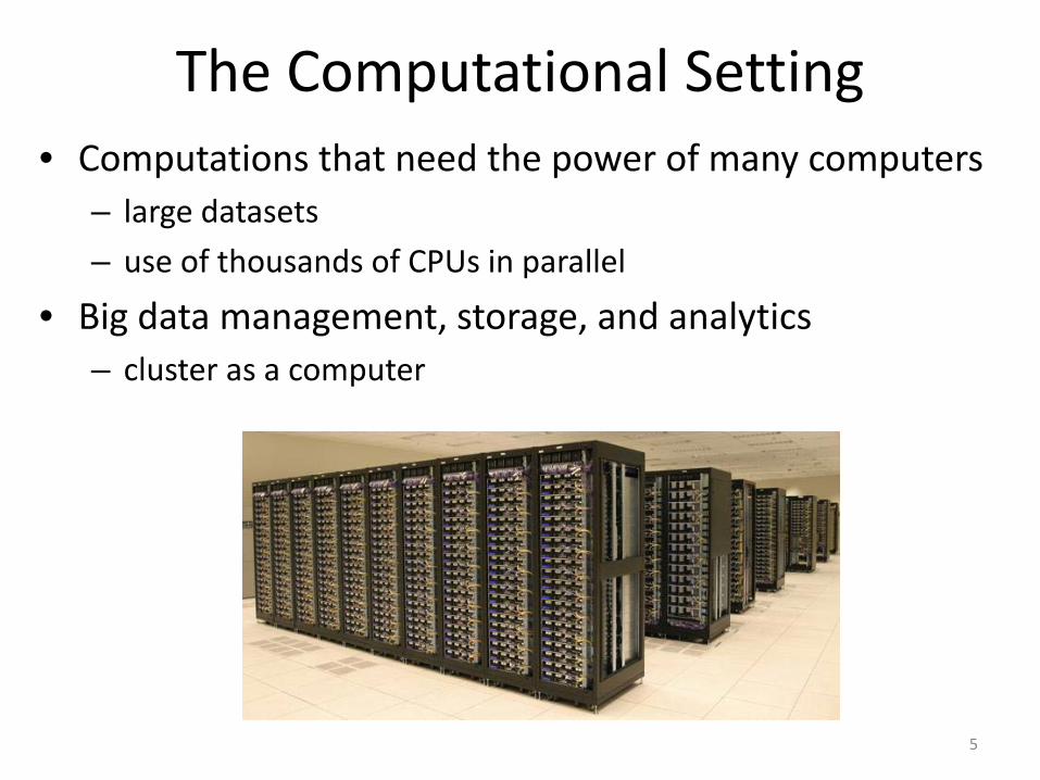
The Computational Setting • Computations that need the power of many computers

– large datasets – use of thousands of CPUs in parallel

• Big data management, storage, and analytics – cluster as a computer

5

MapReduce & Hadoop: Historical Background • 2003: Google publishes about its cluster architecture & distributed file

system (GFS) • 2004: Google publishes about its MapReduce programming model used

on top of GFS – both GFS and MapReduce are written in C++ and are closed-source, with

Python and Java APIs available to Google programmers only • 2006: Apache & Yahoo! -> Hadoop & HDFS

– open-source, Java implementations of Google MapReduce and GFS with a diverse set of APIs available to public

– evolved from Apache Lucene/Nutch open-source web search engine (Nutch MapReduce and NDFS)

• 2008: Hadoop becomes an independent Apache project – Yahoo! uses Hadoop in production

• Today: Hadoop is used as a general-purpose storage and analysis platform for big data – other Hadoop distributions from several vendors including EMC, IBM,

Microsoft, Oracle, Cloudera, etc. – many users (http://wiki.apache.org/hadoop/PoweredBy) – research and development actively continues…

6

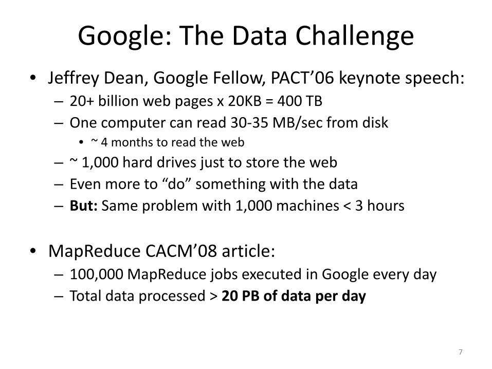
Google: The Data Challenge • Jeffrey Dean, Google Fellow, PACT’06 keynote speech:

– 20+ billion web pages x 20KB = 400 TB – One computer can read 30-35 MB/sec from disk

• ~ 4 months to read the web – ~ 1,000 hard drives just to store the web – Even more to “do” something with the data – But: Same problem with 1,000 machines < 3 hours

• MapReduce CACM’08 article:

– 100,000 MapReduce jobs executed in Google every day – Total data processed > 20 PB of data per day

7

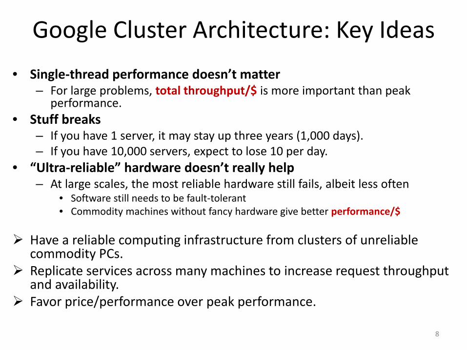
Google Cluster Architecture: Key Ideas • Single-thread performance doesn’t matter

– For large problems, total throughput/$ is more important than peak performance.

• Stuff breaks – If you have 1 server, it may stay up three years (1,000 days). – If you have 10,000 servers, expect to lose 10 per day.

• “Ultra-reliable” hardware doesn’t really help – At large scales, the most reliable hardware still fails, albeit less often

• Software still needs to be fault-tolerant • Commodity machines without fancy hardware give better performance/$

Have a reliable computing infrastructure from clusters of unreliable

commodity PCs. Replicate services across many machines to increase request throughput

and availability. Favor price/performance over peak performance.

8

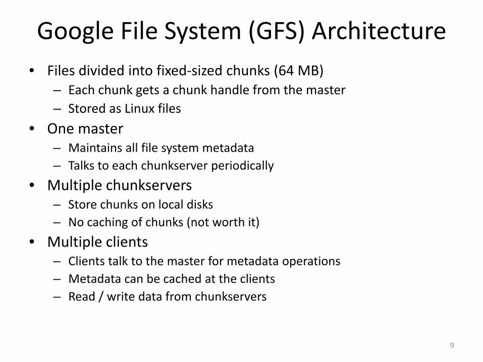
Google File System (GFS) Architecture • Files divided into fixed-sized chunks (64 MB)

– Each chunk gets a chunk handle from the master – Stored as Linux files

• One master – Maintains all file system metadata – Talks to each chunkserver periodically

• Multiple chunkservers – Store chunks on local disks – No caching of chunks (not worth it)

• Multiple clients – Clients talk to the master for metadata operations – Metadata can be cached at the clients – Read / write data from chunkservers

9

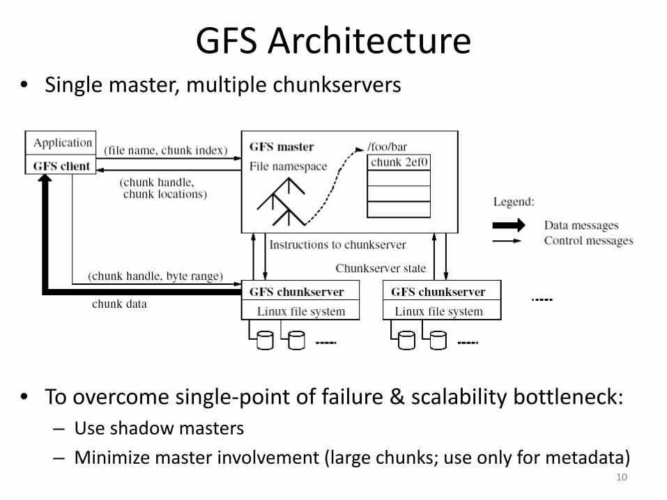
• Single master, multiple chunkservers

• To overcome single-point of failure & scalability bottleneck: – Use shadow masters – Minimize master involvement (large chunks; use only for metadata)

GFS Architecture

10





11

MapReduce

• a software framework first introduced by Google in 2004 to support parallel and fault-tolerant computations over large data sets on clusters of computers

• based on the map/reduce functions commonly used in the functional programming world

12

MapReduce in a Nutshell • Given:

– a very large dataset – a well-defined computation task to be performed on elements of

this dataset (preferably, in a parallel fashion on a large cluster)

• MapReduce framework: – Just express what you want to compute (map() & reduce()). – Don’t worry about parallelization, fault tolerance, data

distribution, load balancing (MapReduce takes care of these). – What changes from one application to another is the actual

computation; the programming structure stays similar.

13

MapReduce in a Nutshell

• Here is the framework in simple terms: – Read lots of data. – Map: extract something that you care about from each record. – Shuffle and sort. – Reduce: aggregate, summarize, filter, or transform. – Write the results.

• One can use as many Maps and Reduces as needed to model a given problem.

14

MapReduce vs. Traditional RDBMS

15

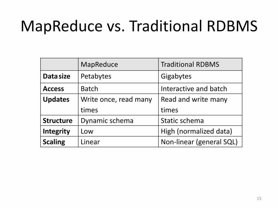
MapReduce

Traditional RDBMS

Data size Petabytes Gigabytes

Access Batch Interactive and batch Updates Write once, read many

times Read and write many times

Structure Dynamic schema Static schema Integrity Low High (normalized data) Scaling Linear Non-linear (general SQL)

Functional Programming Foundations

• map in MapReduce ↔ map in FP • reduce in MapReduce ↔ fold in FP

• Note: There is no precise 1-1 correspondence,

but the general idea is similar.

16

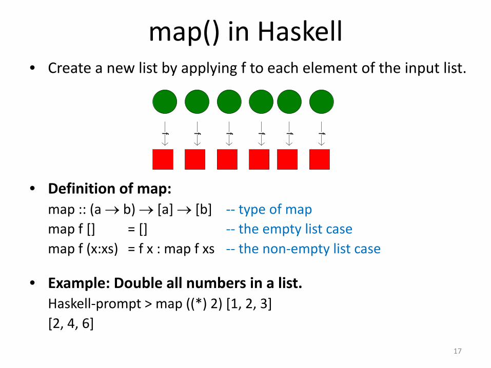
map() in Haskell • Create a new list by applying f to each element of the input list.

• Definition of map: map :: (a → b) → [a] → [b] -- type of map map f [] = [] -- the empty list case map f (x:xs) = f x : map f xs -- the non-empty list case

• Example: Double all numbers in a list. Haskell-prompt > map ((*) 2) [1, 2, 3] [2, 4, 6]

17

f f f f f f

Implicit Parallelism in map()

• In a purely functional setting, an element of a list being computed by map cannot see the effects of the computations on other elements.

• If the order of application of a function f to elements in a list is commutative, then we can reorder or parallelize execution.

• This is the “secret” that MapReduce exploits.

18

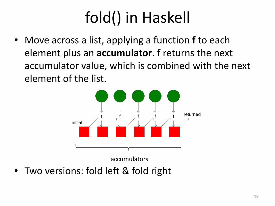
fold() in Haskell • Move across a list, applying a function f to each

element plus an accumulator. f returns the next accumulator value, which is combined with the next element of the list.

• Two versions: fold left & fold right

19

f f f f f returned

initial

accumulators

fold() in Haskell • Definition of fold left: foldl :: (b → a → b) → b → [a] → b -- type of foldl foldl f y [] = y -- the empty list case foldl f y (x:xs) = foldl f (f y x) xs -- the non-empty list case • Definition of fold right: foldr :: (a → b → b) → b → [a] → b -- type of foldr foldr f y [] = y -- the empty list case foldr f y (x:xs) = f x (foldr f y xs) -- the non-empty list case • Example: Compute the sum of all numbers in a list. Haskell-prompt > foldl (+) 0 [1, 2, 3] foldl (+) 0 [1, 2, 3] 6 ⇒ (((0 + 1) + 2) + 3) ⇒ 6

20

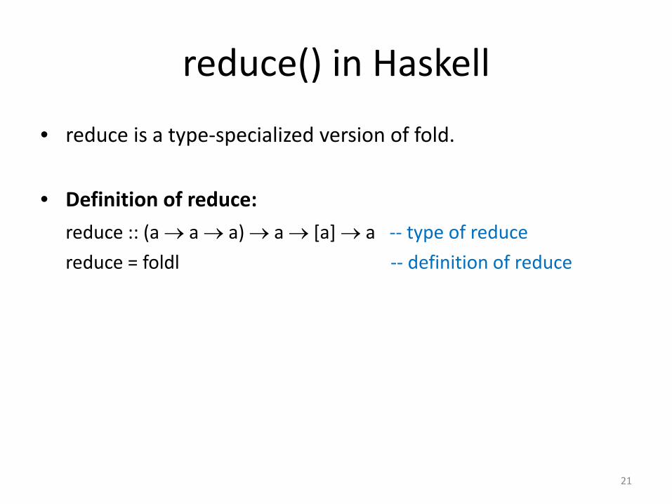
reduce() in Haskell

• reduce is a type-specialized version of fold.

• Definition of reduce: reduce :: (a → a → a) → a → [a] → a -- type of reduce reduce = foldl -- definition of reduce

21

MapReduce Basic Programming Model

• Transform a set of input key-value pairs to a set of output values: – Map: (k1, v1) → list(k2, v2) – MapReduce library groups all intermediate pairs

with same key together. – Reduce: (k2, list(v2)) → list(v2)

22

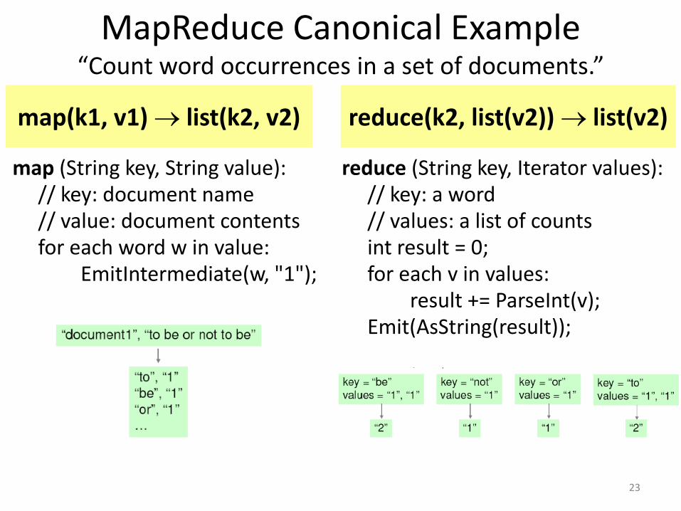
MapReduce Canonical Example “Count word occurrences in a set of documents.”

map (String key, String value): // key: document name // value: document contents for each word w in value: EmitIntermediate(w, "1");

reduce (String key, Iterator values): // key: a word // values: a list of counts int result = 0; for each v in values: result += ParseInt(v); Emit(AsString(result));

23

map(k1, v1) → list(k2, v2) reduce(k2, list(v2)) → list(v2)

MapReduce Parallelization • Multiple map() functions run in parallel, creating

different intermediate values from different input data sets.

• Multiple reduce() functions also run in parallel, each working on a different output key.

• All values are processed independently.

• Bottleneck: The reduce phase can’t start until the map phase is completely finished.

24

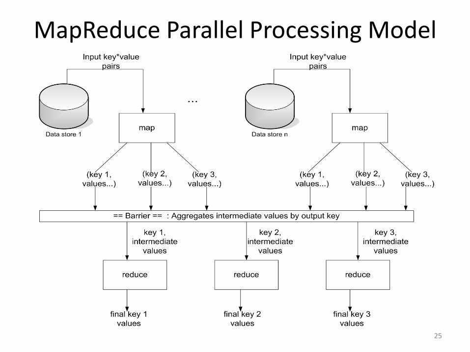
MapReduce Parallel Processing Model

25

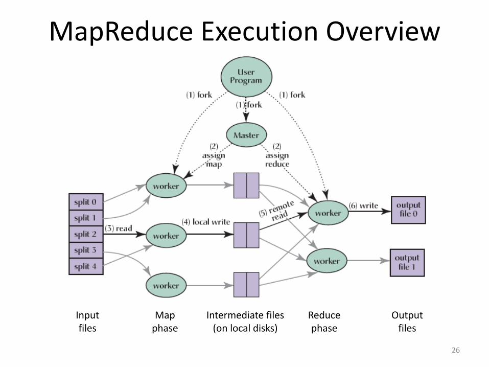
MapReduce Execution Overview

26

Map phase

Reduce phase

Input files

Output files

Intermediate files (on local disks)

MapReduce Scheduling • One master, many workers

– Input data split into M map tasks (typically 64 MB (~ chunk size in GFS)) – Reduce phase partitioned into R reduce tasks (hash(k) mod R) – Tasks are assigned to workers dynamically

• Master assigns each map task to a free worker

– Considers locality of data to worker when assigning a task – Worker reads task input (often from local disk) – Worker produces R local files containing intermediate k/v pairs

• Master assigns each reduce task to a free worker

– Worker reads intermediate k/v pairs from map workers – Worker sorts & applies user’s reduce operation to produce the output

27

Choosing M and R • M = number of map tasks, R = number of reduce tasks • Larger M, R: creates smaller tasks, enabling easier load

balancing and faster recovery (many small tasks from failed machine)

• Limitation: O(M+R) scheduling decisions and O(M*R) in-memory state at master – Very small tasks not worth the startup cost

• Recommendation: – Choose M so that split size is approximately 64 MB – Choose R a small multiple of the number of workers;

alternatively choose R a little smaller than #workers to finish reduce phase in one “wave”

28

MapReduce Fault Tolerance • On worker failure:

– Master detects failure via periodic heartbeats. – Both completed and in-progress map tasks on that worker should

be re-executed (→ output stored on local disk). – Only in-progress reduce tasks on that worker should be re-

executed (→ output stored in global file system). – All reduce workers will be notified about any map re-executions.

• On master failure: – State is check-pointed to GFS: new master recovers & continues.

• Robustness: – Example: Lost 1600 of 1800 machines once, but finished fine.

29

MapReduce Data Locality • Goal: To conserve network bandwidth. • In GFS, data files are divided into 64 MB blocks and 3

copies of each are stored on different machines. • Master program schedules map() tasks based on the

location of these replicas: – Put map() tasks physically on the same machine as one of

the input replicas (or, at least on the same rack / network switch).

• This way, thousands of machines can read input at local disk speed. Otherwise, rack switches would limit read rate.

30

Stragglers & Backup Tasks • Problem: “Stragglers” (i.e., slow workers) significantly

lengthen the completion time. • Solution: Close to completion, spawn backup copies of

the remaining in-progress tasks. – Whichever one finishes first, “wins”.

• Additional cost: a few percent more resource usage. • Example: A sort program without backup = 44% longer.

31

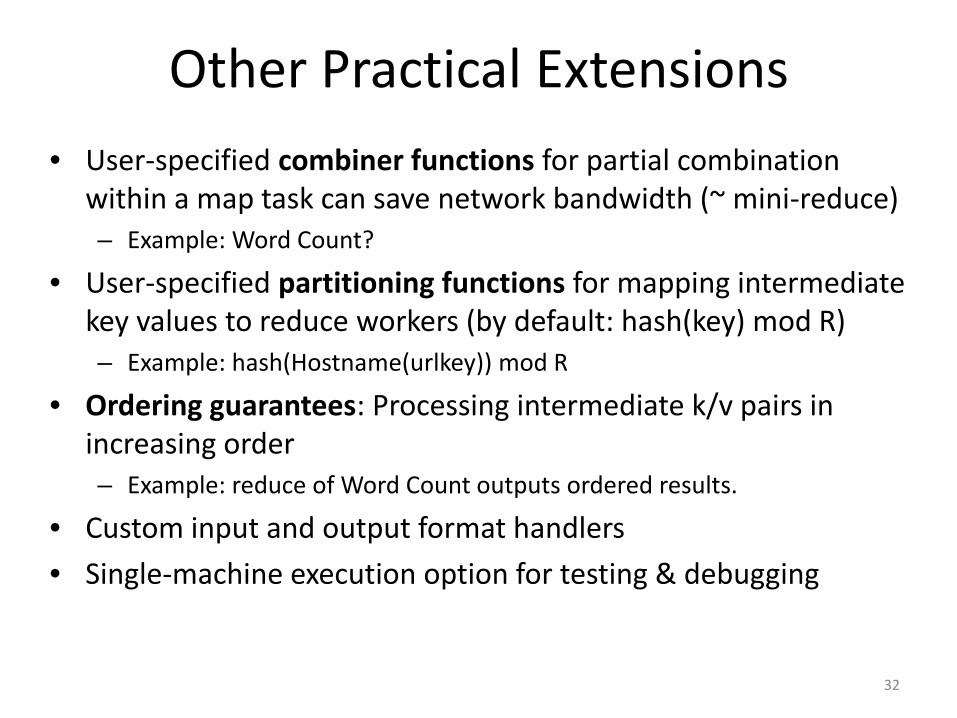
Other Practical Extensions • User-specified combiner functions for partial combination

within a map task can save network bandwidth (~ mini-reduce) – Example: Word Count?

• User-specified partitioning functions for mapping intermediate key values to reduce workers (by default: hash(key) mod R) – Example: hash(Hostname(urlkey)) mod R

• Ordering guarantees: Processing intermediate k/v pairs in increasing order – Example: reduce of Word Count outputs ordered results.

• Custom input and output format handlers • Single-machine execution option for testing & debugging

32

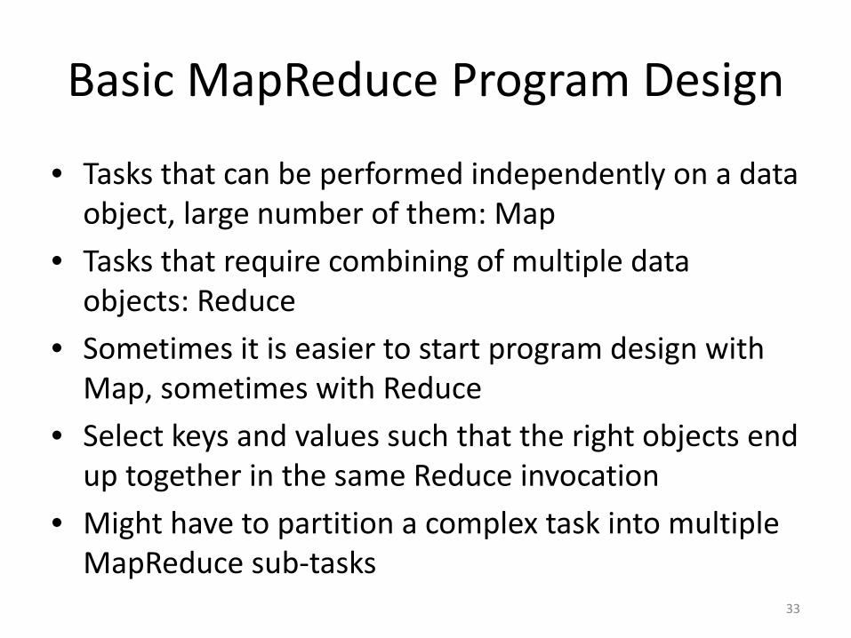
Basic MapReduce Program Design

• Tasks that can be performed independently on a data object, large number of them: Map

• Tasks that require combining of multiple data objects: Reduce

• Sometimes it is easier to start program design with Map, sometimes with Reduce

• Select keys and values such that the right objects end up together in the same Reduce invocation

• Might have to partition a complex task into multiple MapReduce sub-tasks

33





34

What is Hadoop?

• Hadoop is an ecosystem of tools for processing “Big Data”.

• Hadoop is an open source project.

35

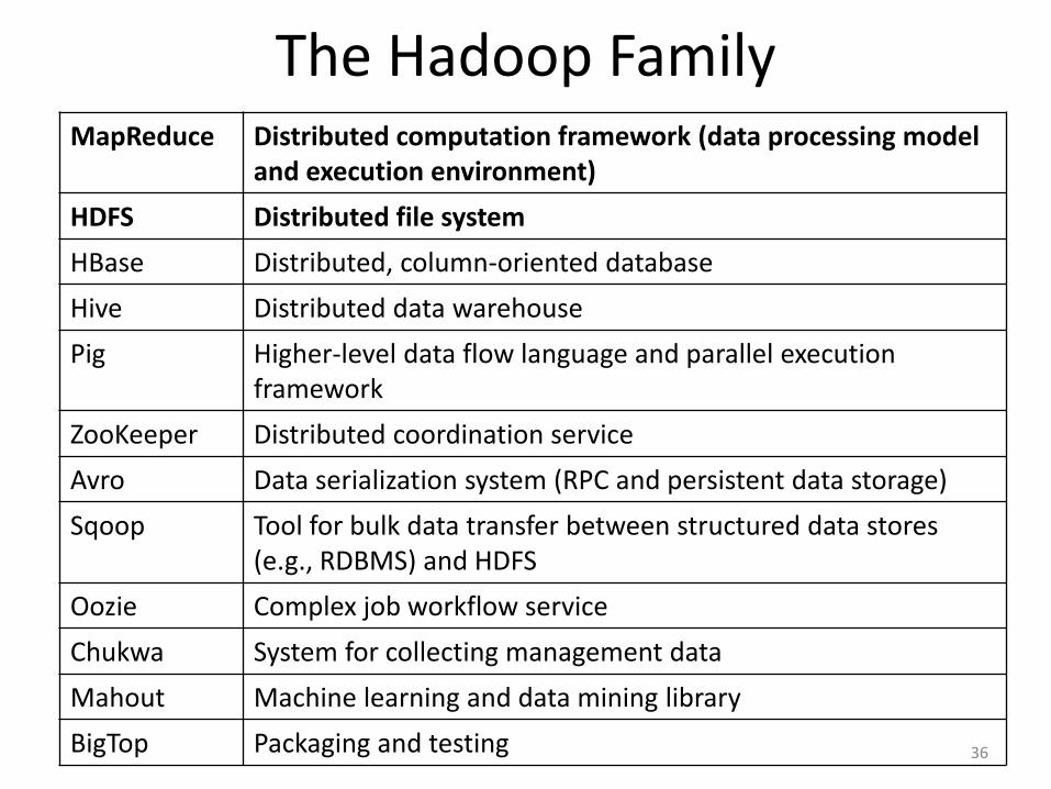
The Hadoop Family MapReduce Distributed computation framework (data processing model

and execution environment) HDFS Distributed file system HBase Distributed, column-oriented database Hive Distributed data warehouse Pig Higher-level data flow language and parallel execution

framework ZooKeeper Distributed coordination service Avro Data serialization system (RPC and persistent data storage) Sqoop Tool for bulk data transfer between structured data stores

(e.g., RDBMS) and HDFS Oozie Complex job workflow service Chukwa System for collecting management data Mahout Machine learning and data mining library BigTop Packaging and testing 36

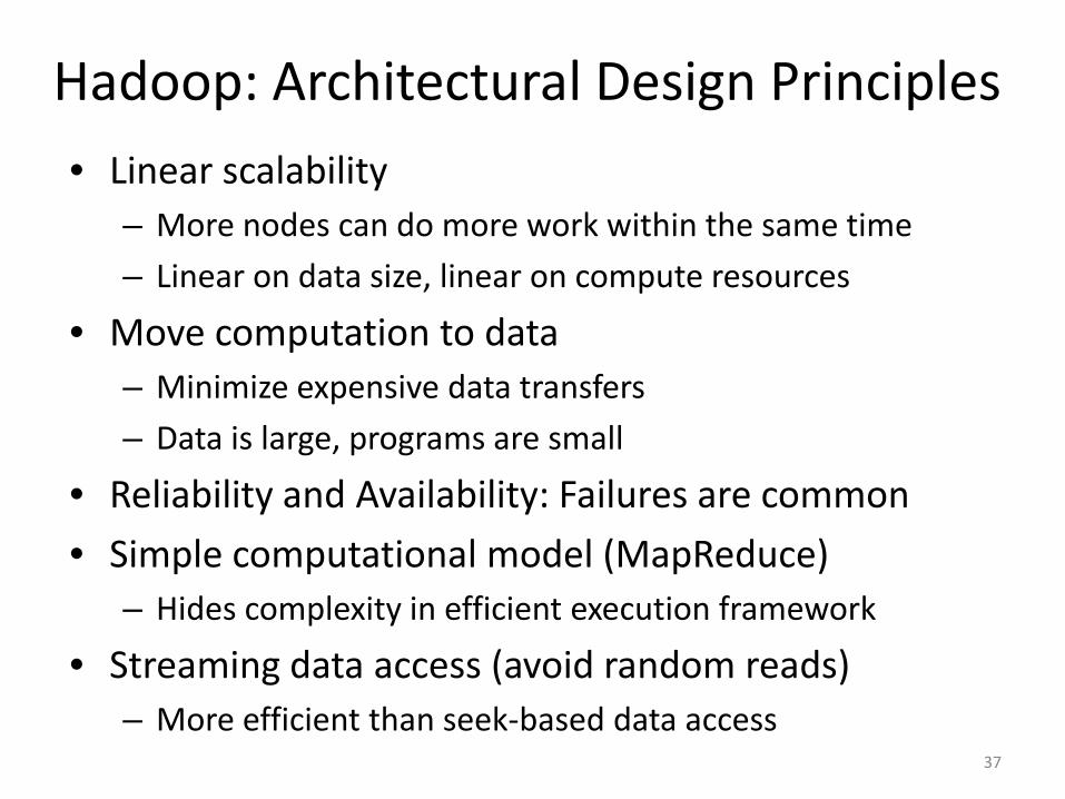
Hadoop: Architectural Design Principles • Linear scalability

– More nodes can do more work within the same time – Linear on data size, linear on compute resources

• Move computation to data – Minimize expensive data transfers – Data is large, programs are small

• Reliability and Availability: Failures are common • Simple computational model (MapReduce)

– Hides complexity in efficient execution framework

• Streaming data access (avoid random reads) – More efficient than seek-based data access

37

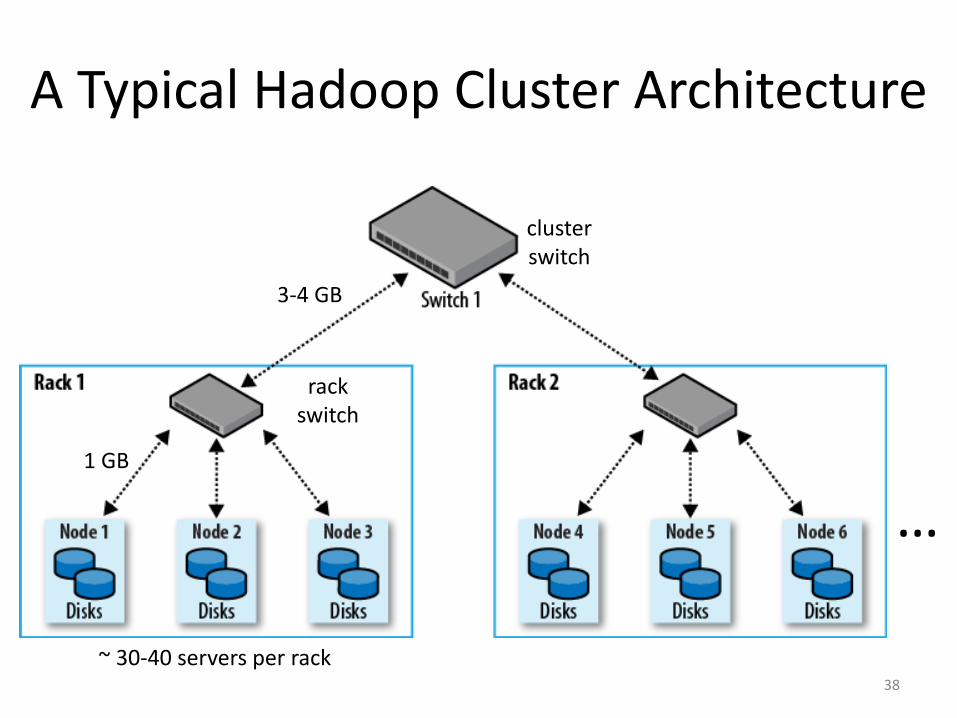
A Typical Hadoop Cluster Architecture

38

cluster switch

rack switch

…

~ 30-40 servers per rack

1 GB

3-4 GB

Hadoop Main Cluster Components • HDFS daemons

– NameNode: namespace and block management (~ master in GFS) – DataNodes: block replica container (~ chunkserver in GFS)

• MapReduce daemons – JobTracker: client communication, job scheduling, resource

management, lifecycle coordination (~ master in Google MR) – TaskTrackers: task execution module (~ worker in Google MR)

NameNode JobTracker

TaskTracker TaskTracker TaskTracker

DataNode DataNode DataNode 39

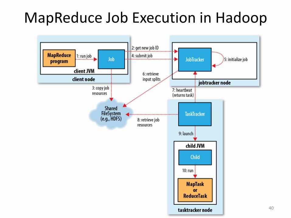
MapReduce Job Execution in Hadoop

40

Job Submission (1-4)

• Client submits MapReduce job through Job.submit() call

• Job submission process – Get new job ID from JobTracker – Determine input splits for job – Copy job resources (job JAR file, configuration file,

computed input splits) to HDFS into directory named after the job ID

– Inform JobTracker that job is ready for execution

41

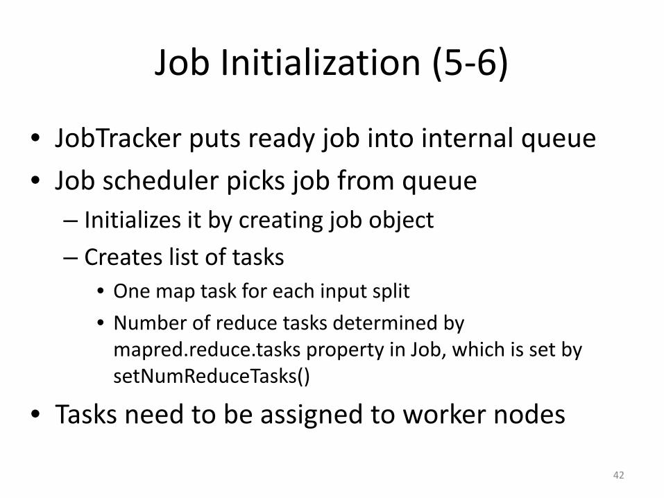
Job Initialization (5-6)

• JobTracker puts ready job into internal queue • Job scheduler picks job from queue

– Initializes it by creating job object – Creates list of tasks

• One map task for each input split • Number of reduce tasks determined by

mapred.reduce.tasks property in Job, which is set by setNumReduceTasks()

• Tasks need to be assigned to worker nodes

42

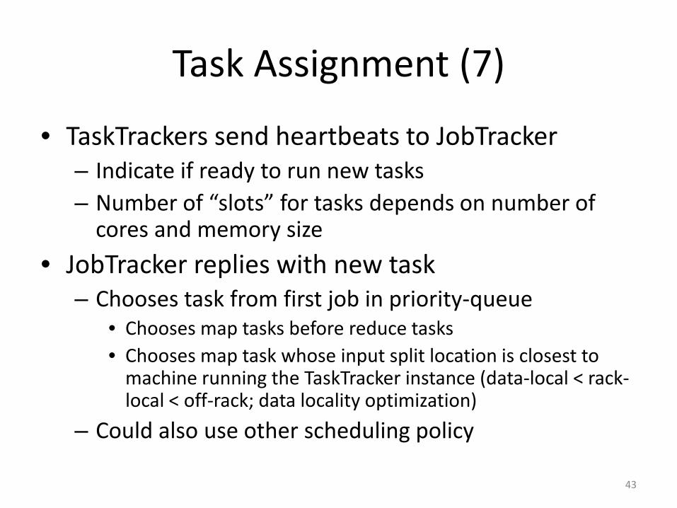
Task Assignment (7)

• TaskTrackers send heartbeats to JobTracker – Indicate if ready to run new tasks – Number of “slots” for tasks depends on number of

cores and memory size • JobTracker replies with new task

– Chooses task from first job in priority-queue • Chooses map tasks before reduce tasks • Chooses map task whose input split location is closest to

machine running the TaskTracker instance (data-local < rack-local < off-rack; data locality optimization)

– Could also use other scheduling policy

43

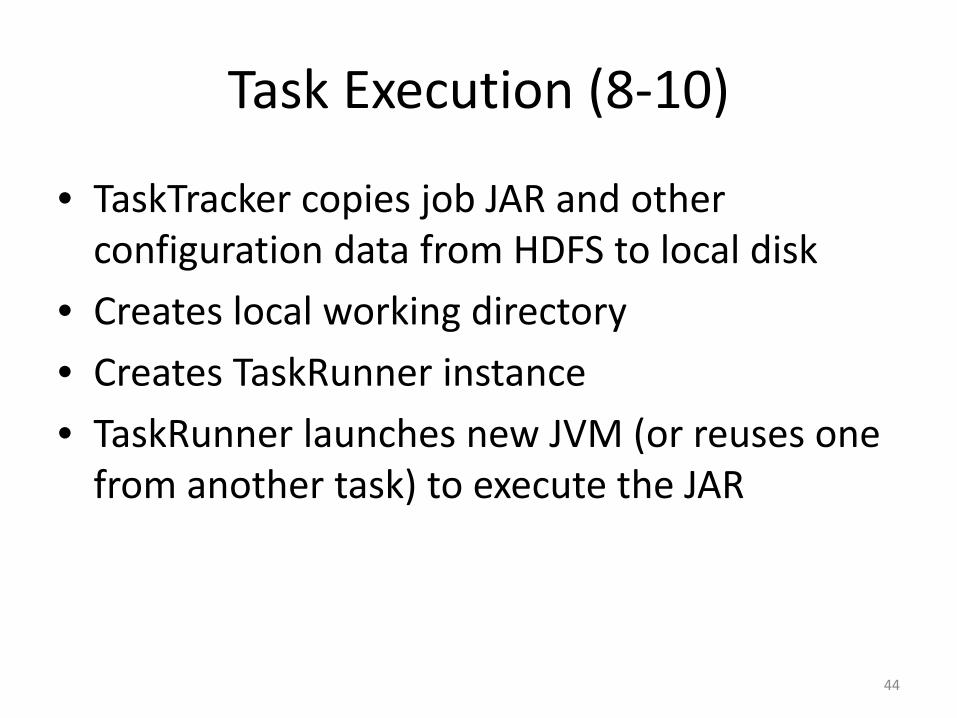
Task Execution (8-10)

• TaskTracker copies job JAR and other configuration data from HDFS to local disk

• Creates local working directory • Creates TaskRunner instance • TaskRunner launches new JVM (or reuses one

from another task) to execute the JAR

44

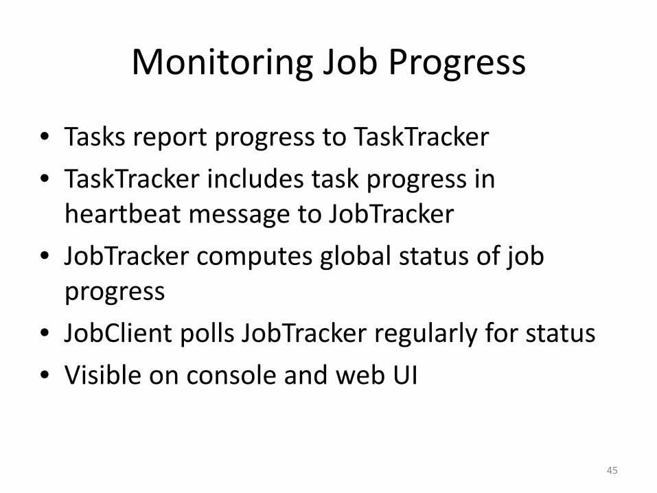
Monitoring Job Progress

• Tasks report progress to TaskTracker • TaskTracker includes task progress in

heartbeat message to JobTracker • JobTracker computes global status of job

progress • JobClient polls JobTracker regularly for status • Visible on console and web UI

45

Handling Task Failures

• Error reported to TaskTracker and logged • Hanging task detected through timeout • JobTracker will automatically re-schedule

failed tasks – Tries up to mapred.map.max.attempts many times

(similar for reduce) – Job is aborted when task failure rate exceeds

mapred.max.map.failures.percent (similar for reduce)

46

Handling TaskTracker & JobTracker Failures

• TaskTracker failure detected by JobTracker from missing heartbeat messages – JobTracker re-schedules map tasks and not

completed reduce tasks from that TaskTracker

• Hadoop cannot deal with JobTracker failure – Could use Google’s proposed JobTracker take-over

idea, using ZooKeeper to make sure there is at most one JobTracker

– Improvements in progress in newer releases…

47

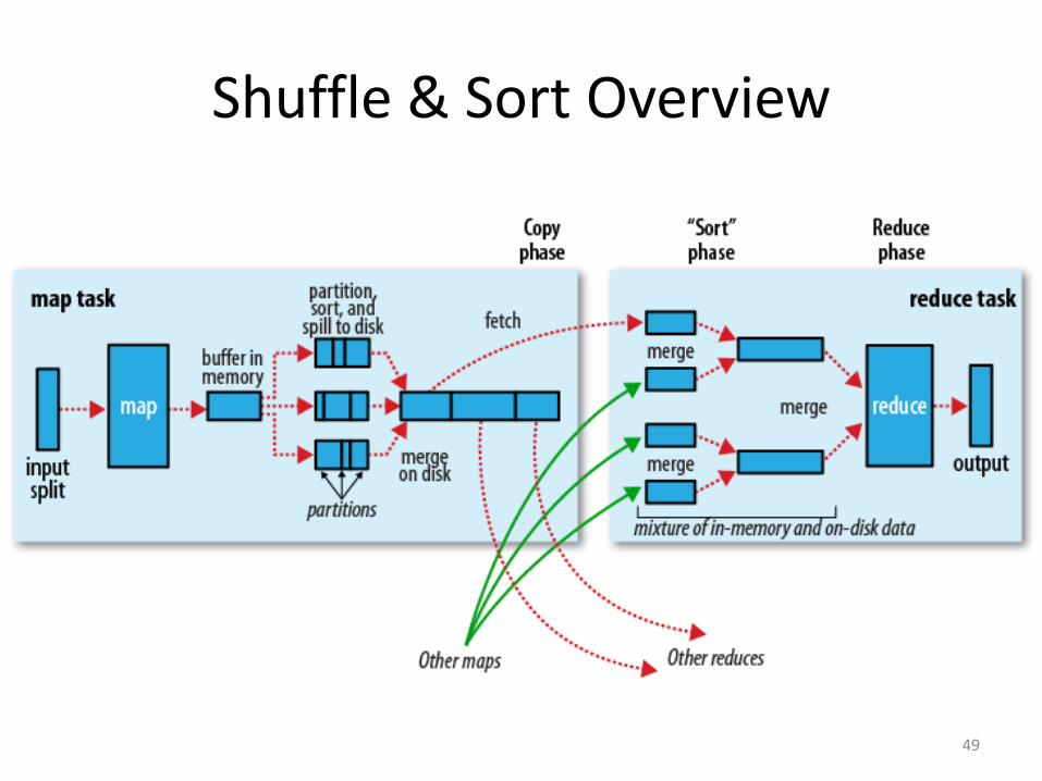
Moving Data from Mappers to Reducers

• “Shuffle & Sort” phase – synchronization barrier between map and reduce phase – one of the most expensive parts of a MapReduce

execution

• Mappers need to separate output intended for different reducers

• Reducers need to collect their data from all mappers and group it by key – keys at each reducer are processed in order

48

Shuffle & Sort Overview

49

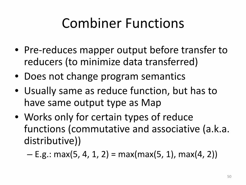
Combiner Functions

• Pre-reduces mapper output before transfer to reducers (to minimize data transferred)

• Does not change program semantics • Usually same as reduce function, but has to

have same output type as Map • Works only for certain types of reduce

functions (commutative and associative (a.k.a. distributive)) – E.g.: max(5, 4, 1, 2) = max(max(5, 1), max(4, 2))

50

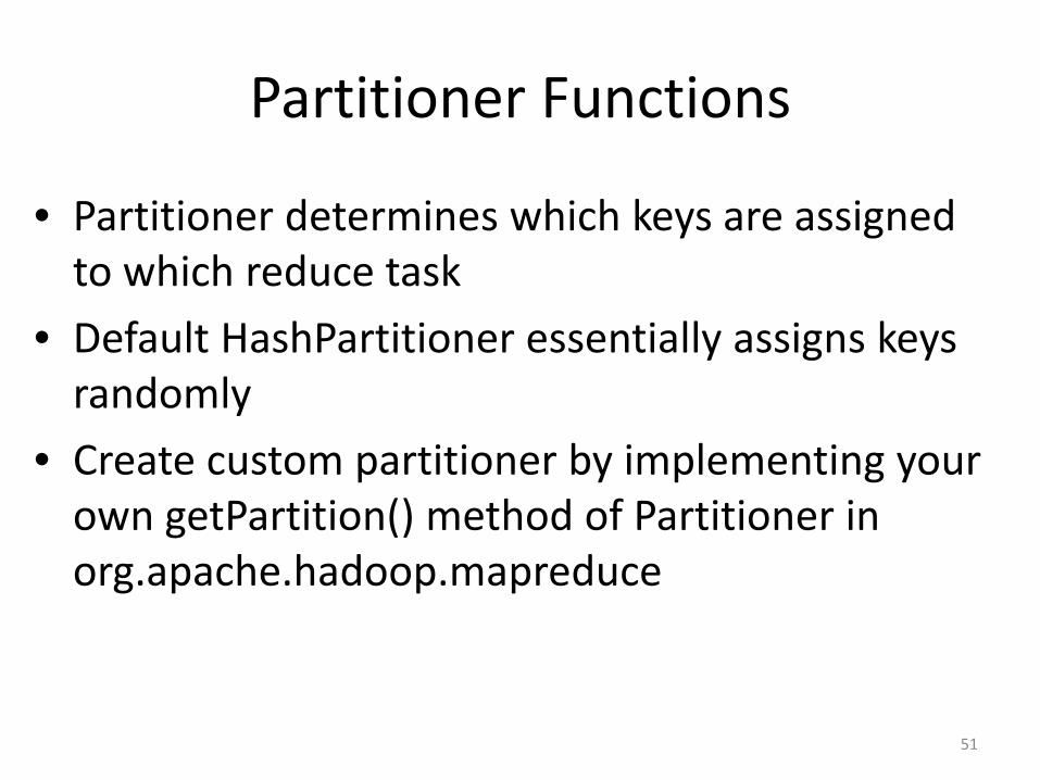
Partitioner Functions

• Partitioner determines which keys are assigned to which reduce task

• Default HashPartitioner essentially assigns keys randomly

• Create custom partitioner by implementing your own getPartition() method of Partitioner in org.apache.hadoop.mapreduce

51

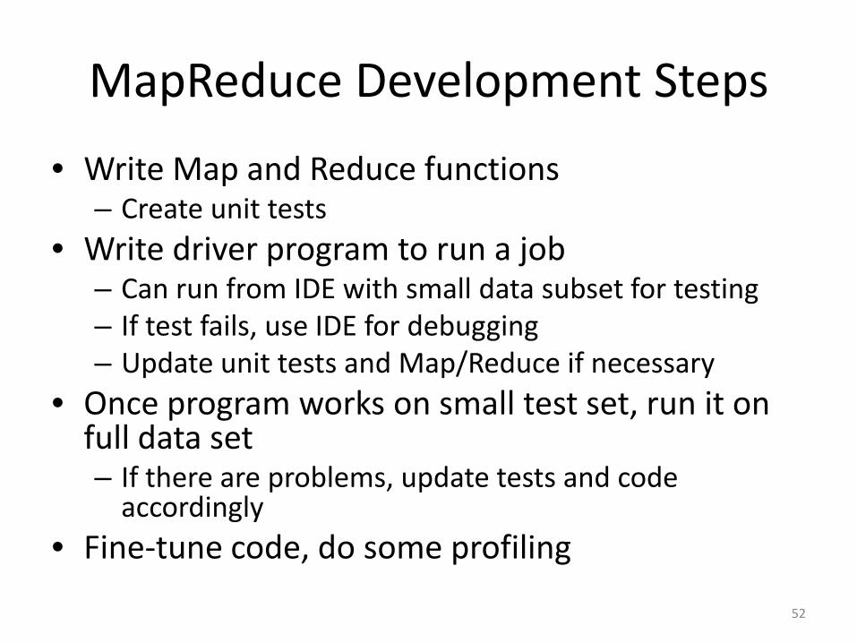
MapReduce Development Steps

• Write Map and Reduce functions – Create unit tests

• Write driver program to run a job – Can run from IDE with small data subset for testing – If test fails, use IDE for debugging – Update unit tests and Map/Reduce if necessary

• Once program works on small test set, run it on full data set – If there are problems, update tests and code

accordingly • Fine-tune code, do some profiling

52

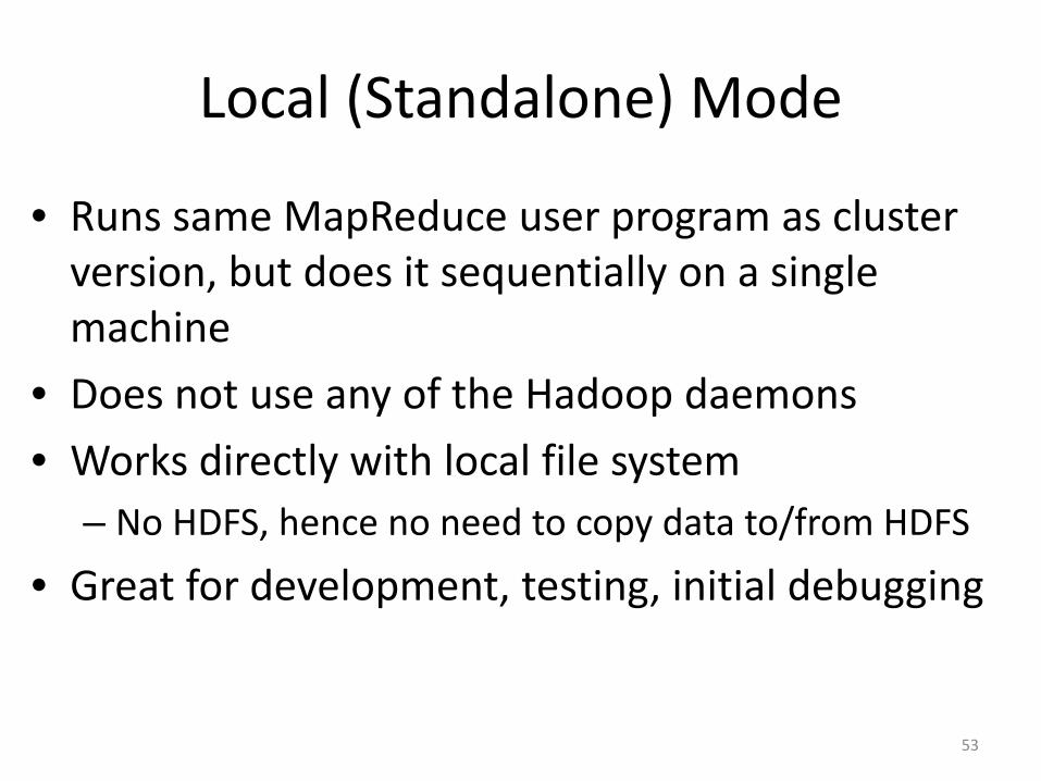
Local (Standalone) Mode

• Runs same MapReduce user program as cluster version, but does it sequentially on a single machine

• Does not use any of the Hadoop daemons • Works directly with local file system

– No HDFS, hence no need to copy data to/from HDFS

• Great for development, testing, initial debugging

53

Pseudo-Distributed Mode

• Still runs on a single machine, but simulating a real Hadoop cluster – Simulates multiple nodes – Runs all daemons – Uses HDFS

• For more advanced testing and debugging • You can also set this up on your laptop

54

Programming Language Support

• Java API (native) • Hadoop Streaming API

– allows writing map and reduce functions in any programming language that can read from standard input and write to standard output

– Examples: Ruby, Python

• Hadoop Pipes API – allows map and reduce functions written in C++ using

sockets to communicate with Hadoop’s TaskTrackers

55


• Motivation • Google MapReduce • The Hadoop Ecosystem



56

Hadoop Distributed File System (HDFS)

• Distributed file systems manage the storage across a network of machines.

• Hadoop has a general-purpose file system abstraction (i.e., can integrate with several storage systems such as the local file system, HDFS, Amazon S3, etc.).

• HDFS is Hadoop’s flagship file system.

57

HDFS Design • Very large files • Streaming data access

– write-once, read-many-times pattern – time to read the whole dataset is more important

• Commodity hardware – fault-tolerance

• HDFS is not a good fit for – low-latency data access – lots of small files – multiple writers, arbitrary file modifications

58

Blocks

• HDFS files are broken into block-sized chunks (64 MB by default)

• With the (large) block abstraction: – a file can be larger than any single disk in the

network – storage subsystem is simplified (e.g., metadata

bookkeeping) – replication for fault-tolerance and availability is

facilitated

59

Namenodes and Datanodes • Two types of HDFS nodes:

– one Namenode (the master) – multiple Datanodes (workers)

• Namenode manages the filesystem namespace. – file system tree and metadata, stored persistently – block locations, stored transiently

• Datanodes store and retrieve data blocks when they are told to by clients or the Namenode.

• Datanodes report back to the Namenode periodically with lists of blocks that they are storing.

60

HDFS Federation & High-Availability

• In latest releases of Hadoop: – HDFS Federation allows multiple Namenodes, each

of which manages a portion of the file system namespace; the goal is to enhance the scalability of the Namenode on very large clusters with many files and blocks.

– HDFS High-Availability provides faster recovery from Namenode failures using a pair of namenodes in an active standby configuration.

61

Reading from HDFS

62

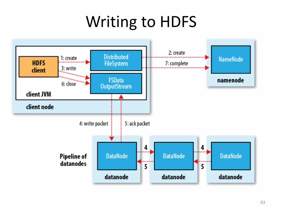
Writing to HDFS

63

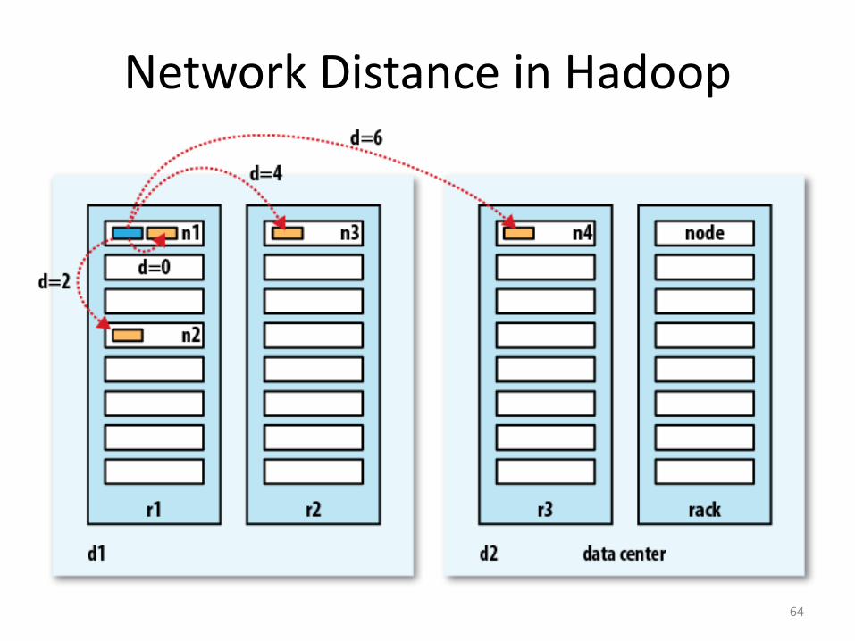
Network Distance in Hadoop

64

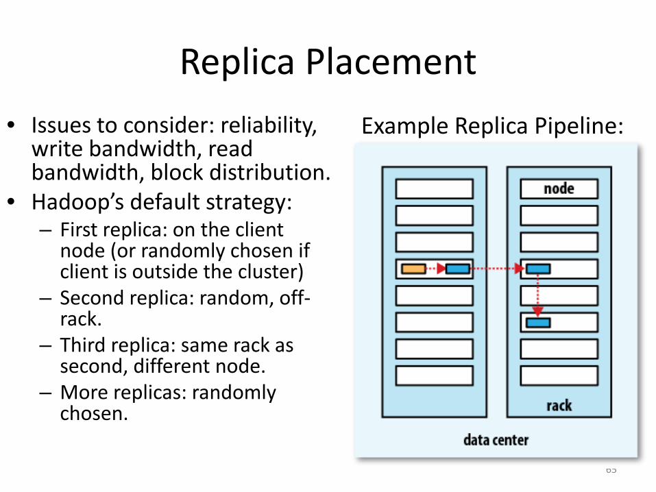
Replica Placement • Issues to consider: reliability,

write bandwidth, read bandwidth, block distribution.

• Hadoop’s default strategy: – First replica: on the client

node (or randomly chosen if client is outside the cluster)

– Second replica: random, off-rack.

– Third replica: same rack as second, different node.

– More replicas: randomly chosen.

65

Example Replica Pipeline:

Coherency Model • Coherency model describes the data visibility of

reads and writes for a file. • In HDFS:

– The metadata for a newly created file is visible in the file system namespace.

– The current data block being written is not guaranteed to be visible to other readers.

• To force all buffers to be synchronized to all relevant datanodes, you can use the sync() method.

• Without sync(), you may lose up to a block of (newly written) data in the event of client or system failure.

66

Tools for Ingesting Data into HDFS

• Apache Flume – to move large quantities of streaming data into

HDFS (e.g., log data from a system)

• Apache Sqoop – to perform bulk imports of data into HDFS from

structured data stores, such as relational databases

67

References • “Web Search for a Planet: The Google Cluster Architecture”, L. Barroso, J.

Dean, U. Hoelzle, IEEE Micro 23(2), 2003. • “The Google File System”, S. Ghemawat, H. Gobioff, S. Leung, SOSP 2003. • “MapReduce: Simplified Data Processing on Large Clusters”, J. Dean, S.

Ghemawat, OSDI 2004 (follow-up papers: CACM 2008, CACM 2010). • “The Hadoop Distributed File System”, K. Shvachko et al, MSST 2010. • “Hadoop: The Definitive Guide”, T. White, O’Reilly, 3rd edition, 2012.

68

big data - systems group · – evolved from apache lucene/nutch open-source web search engine ......

Documents