Big Bang Nucleosynthesis 

The emergence of elements in the universe 

Benjamin Topper 

 

 

 

 

Abstract. 

In this paper, I will first give a brief overview of what general relativity has to say about cosmology, getting an expanding universe as a solution to Einstein's equation, i.e. a universe with a [thermal] history. We will go through the different steps of the big bang nucleosynthesis, briefly justifying the particle‐antiparticle asymmetry (otherwise no nucleosynthesis would happen) and then evaluating and discussing in details the abundances of the first elements. I will then discuss the consequences of the Big Bang B nucleosynthesis on modern physics: the constraints it gives on the standard model, on dark matter...   

 

Contents 

 

1. Introduction to standard cosmology . The Friedmann‐Lemaitre‐Robertson‐Walker models . Thermal history of the universe  

2. Big Bang Nucleosynthesis . Nuclear equilibrium . Weak interaction freeze‐out 

. Element synthesis: Primordial abundances of , , Deuterium,  . 

. Uncertainties  

3. Constraints on new physics . Number of neutrino generations . Neutrino masses . Dark matter  

4. Conclusion 

 

 

 

 

Disclaimer. This lecture is mainly based on Jean Philippe Uzan and Patrick Peter’s book “Cosmologie Primordiale” (chapter4), Mark Trodden and Sean Carroll’s “TASI Lectures : Introduction to Cosmology”, and the review article “Big Bang nucleosynthesis and physics beyond the Standard Model”. The complete list of references used can be found on the last page of this document. 

 

 

 

Introduction to standard cosmology 

The first cosmological solutions to Einstein’s equations were given by Einstein himself in the early 1917. However the general solutions were independently found by Alexandre Friedmann and Georges Lemaitre only in 1922 and 1927. 

The standard Big Bang cosmological model is based on what is now called the “Cosmological Principle”, which assumes that the universe is spatially homogeneous and isotropic. This principle enforces the geometry of the universe to be one that is described by Friedmann and Lemaitre solutions to Einstein’s equations. 

a)  The Friedmann‐Lemaitre‐Robertson‐Walker models 

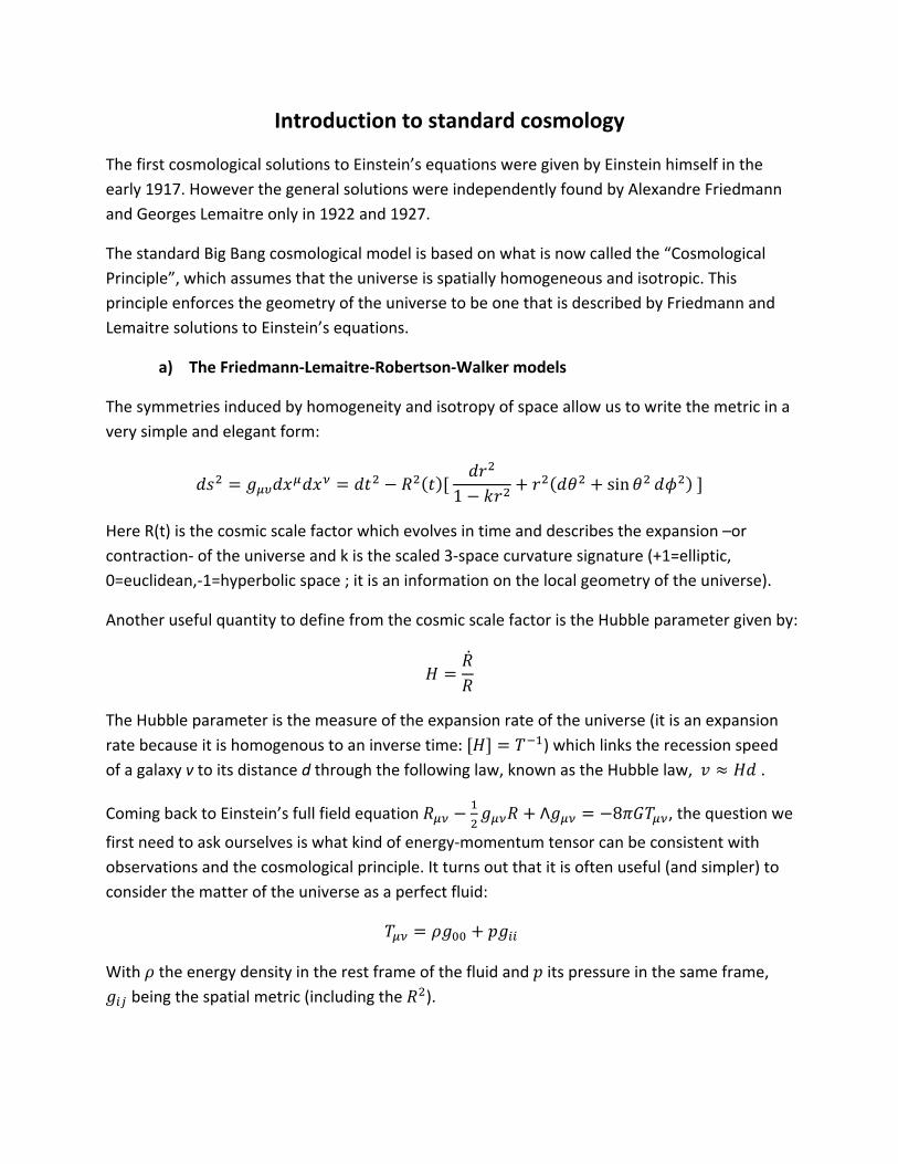
The symmetries induced by homogeneity and isotropy of space allow us to write the metric in a very simple and elegant form: 

1 sin  

Here R(t) is the cosmic scale factor which evolves in time and describes the expansion –or contraction‐ of the universe and k is the scaled 3‐space curvature signature (+1=elliptic, 0=euclidean,‐1=hyperbolic space ; it is an information on the local geometry of the universe). 

Another useful quantity to define from the cosmic scale factor is the Hubble parameter given by: 

 

The Hubble parameter is the measure of the expansion rate of the universe (it is an expansion rate because it is homogenous to an inverse time: ) which links the recession speed of a galaxy v to its distance d through the following law, known as the Hubble law,   . 

Coming back to Einstein’s full field equation Λ 8first need to ask ourselves is what kind of energy‐momentum tensor can be consistent with 

 

 

With   the energy density in the rest frame of the fluid and   its pressure in the same frame, 

, the question we 

observations and the cosmological principle. It turns out that it is often useful (and simpler) toconsider the matter of the universe as a perfect fluid:  

 being the spatial metric (including the ). 

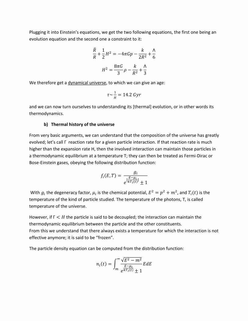
Plugging it into Einstein’s equations, we get the two following equations, the first one being an evolution equation and the second one a constraint to it: 

12 4 2

Λ6 

83

Λ3 

We therefore get a dynamical universe, to which we can give an age:  

~ 14.2

,

  

and we can now turn ourselves to understanding its [thermal] evolution, or in other words its thermodynamics. 

b) Thermal history of the universe 

From very basic arguments, we can understand that the composition of the universe has greatly evolved; let’s call Γ  reaction rate for a given particle interaction. If that reaction rate is much higher than the expansion rate H, then the involved interaction can maintain those particles in a thermodynamic equilibrium at a temperature T; they can then be treated as Fermi‐Dirac or Bose‐Einstein gases, obeying the following distribution function: 

1 

 With  the degeneracy factor,   is the chemical potential, , and   is the  of the photon  call

However, if Γ the particle is said to be decoupled; the interaction can maintain the mic eq

interaction is not 

The particle density equation can be computed from the distribution function: 

√

temperature of the kind of particle studied. The temperature s, T, is ed temperature of the universe. 

thermodyna uilibrium between the particle and the other constituents. From this we understand that there always exists a temperature for which the effective anymore; it is said to be “frozen”. 

1

∞

 

 

This equation, applied to bosons and fermions at different temperatures, gives the following table:  

Limit  Type of particle  n 

,       

     Bosons gζ 3π

T  

    Fermions 

3gζ 34π T  

     

      Bosons  g

mT2π e

E μT  

gmT2π

    Fermions  e

E μT  

Table 1: Thermodynamics 

The photons are known to have zero chemical potential (as the number of photons is not 

conserved), therefore the particle‐antiparticle annihilation process:  must satisfy the following conservation law: . Plugging this in the particle density equation, we find an asymmetry in the number of particles and antiparticles:  

0

Note: at low temperature ( ) we get, as expected, an exponential suppression of this asymmetry that goes 

  

with . 

like . 

This asymmetry explains the domination of matter over antimatter and therefore allows the 

The early universe being dominated by radiation, we can rewrite, using [table 1] the expansion rate of 

83

formation of nuclei. 

expansion of the universe: 

30  

 

 

H being homogenous to an inverse time, we can rewrite it as: 

2.42 

with T in MeV,  being the number of relativistic degrees of freedom at a given temperature. The synopsis of the Big Bang nucleosynthesis can be split into three major phases: 

T >> 1 MeV  Thermodynamic equilibrium between all the components of the universe ; 

Universes dominated by radiation ; ##

~  

Photodissociation prevents any complex nuclei to form.  1>T >0.7Mev  Weak interaction cannot maintain equilibrium between all particles; neutrons 

decouple: “neutron freeze‐out”:##

~  . Free neutrons decay into 

protons; atomic nuclei stay at thermodynamic equilibrium. Freeze‐out temperature . 

0.7>T>0.05Mev  Nuclear thermodynamic equilibrium cannot be maintained. Electron‐positron annihilation has heated the photon bath. Atomic nuclei form through 2‐body collisions:   (only one way because radiation density is low enough). 

Table 2: Thermal evolution of the universe 

 

 

 

 

 

 

 

 

 

 

Big Bang Nucleosynthesis 

a) Nuclear equilibrium   

For temperatures greater or of the order of 100Mev, the universe is dominated by relativistic particles in equilibrium: electrons, positrons, neutrinos and photons. The contribution from non‐relativistic particle can be neglected; the weak interactions between neutrons, protons and leptons: 

 

 

 

keep all the particles (as well as the non‐relativistic baryons) in thermodynamic equilibrium. 

At temperatures larger than 1Mev, the nuclear interactions still maintain the very first nuclei in 

fore given by: 

nA gA mAT2π

 

and the electromagnetic interaction between electrons and positrons: 

thermodynamic equilibrium – their fraction can therefore be computed only using thermodynamic considerations, as shown below. The density of those non‐relativistic nuclei is there

eA A

Tμ

gA mAT2π e

AT e

μT Z e

μT A Z 

 with μ , μ the chemical potential of protons and neutrons.  

g as t e chemical equilibrium imposes 

μA μ A Z μ   

 eglecting the difference in mass between protons and neutrons in the prefactor, we can 

/ 2 2

As lon he reaction rates are higher the expansion rate, ththe chemical potential to be: 

Nextract from this formula the density ratio of protons and neutrons: 

2

/ /

/

 

Rewriting the exponential in the nuclear density, we get: 

nA gA mAT2π e

AT gA

mAT2π 2 AnZnA Z π

mNT

/e

BAT  

 ith   is the binding energy of the nucleon. W

Defining ,  ,  abundances of 

uclei in ermodynamic equilibrium:  

/

∑   , we finally obtain the 

atomic n  th

32

/

 

 

with   the baryon to photon ratio. 

We can use this formula to  e bindi nd the temperature at 

     

get th ng energy of the light nuclei awhich their abundance will be at a maximum:    

  2.22  6.92  7.72  28.3    0.066  0.1  0.11  0.28 

 In particular, it gives the exact good primordial evolution for the Deuterium abundance up to its 

le we understand that even at thermal equilibrium, nucleosynthesis cannot start 

b) Weak interaction freeze‐out and neutron abundance  

t some stage , X can be said to freeze‐out if its abundance stops evolving greatly. on rea rium: 

7π60

peak, and for the other light until elements until they depart from equilibrium (we’ll discuss this point later). From this tabbefore T=0.3MeV. Thermal photons prevent formation of large quantity of deuterium until T>0.3MeV (photodissociation) even though the cross section for  is high.   

 AWeak interacti ction rate for     keeps protons and neutrons in equilib

Γ 1 A F

 ut when this reaction rate becomes of the order of the expansion rate, the thermal 

H

3g G T  

Bequilibrium is broken : 

Γ T0.8 T 0.8MeV or t 1.15s 

Therefore, when the weak interaction (i.e. the neutron abundance) freezes out, the neutron to 

T1

1 T

proton ration is: 

1/6 

Just considering the expansion to get  e neutron abundance at the beginning of icle it will 

e 

6

thnucleosynthesis is a bit too naïve though, ), as the free neutron is not a stable partdecay with a lifetime of 887s from the time weak interaction freezes out to  , temperaturthat allows Deuterium to form (T=0.086MeV, t=180sec). We therefore get :  

1 / 0.136  

c) Element synthesis: Primordial abundances of , , Deuterium,   

utrons are locked up and no heavier  any 

ore e 

synthesis is that no   elements exist with

Let’s start our analysis with qualitative arguments: The formation of deuterium is a crucial factor for the continuation of the Big Bang nucleosynthesis: if too much   is formed, then neelements can be created. However if too little is formed, then an important factor infurther fusion is missing; especially, when deuterium can form, helium4 can form much measily because the following reactions   and    enable thcreation of large amounts for Helium through  and  .  A very important factor in the Big Bang nucleo stable  A=5 and A=8 (figure 4). Therefore we would expect  to greatly this “anomaly”  decrease any 

lium ndance than Helium‐4 (tritium is 

t 

 

 Figure 1: Nuclear reactions ‐ http://physicsworld.com/cws/article/print/30680/1/PWfea4_08‐07 

nucleation process at A=4 and A=7 (it is a lot less likely for A=4 to go to A=6 than to A=5).  From this, we understand that: 

• The abundance of  should at first increase then decrease when Helium‐4 can be onsumed in the reactions). produced (as it is being c

• The abundances of  and  should increase then level up or decrease when heis getting created. They should have a lower final abu

e sh  decradioactive therefor ould rease over long periods –longer than the one studied here) 

• Helium‐4, which is stable, and at the end of the “first chain” (before A=5) should be present in large quantities at the end of the Big Bang nucleosynthesis. All the previous elements can fuse to form Helium‐4, and Helium‐4 is very unlikely (but not 0) to reacwith protons or neutrons to jump to A=6 

• Abundances of Lithium and Beryllium should be very low compared to the other. We can expect   and   to be the end of the Big Bang nucleosynthesis because of theA=8 “barrier” (also helped by the fact that Be7 is radioactive and therefore decays to lighter elements). 

• Lithium valley:  destroyed by protons but Be7 contribution. 

Now let’s get into some little computations: The easiest estimation is for Helium‐4: we now that all free neutrons left after freeze‐out will get bound up to He‐4 because of nuclei stability. Estimations on He‐4 abundances depend mostly on the neutron to proton rate, thus most of the uncertainties are based on the uncertainties of the free neutron lifetime (τ= 887 seconds)  

~ 21 0.24  

For Deuterium, we can get its creation slope with the thermal‐equilibrium equation given previously (simply using Mathematica, it work perfectly); however getting its final abundance is much more difficult as we have to compute all its “sink terms”. The same problem appears for all the other elements. It is however doable without a computer, starting with the very general statement: 

Γ  

where J(t) and  Γ  are time‐dependant source and sink terms. The solution to this equation is 

Γ Γ 

This requires, as expected, careful examination of all the different reaction networks and keeping track of their reaction rate as temperature decreases, therefore it is a very tedious 

Γ

computation (figure 2)1.  Generally freeze‐out occurs when Γ~ . It is possible to show that X approaches this equilibrium 

value for  ∞  

 Figure 2: Analytic computation 

http://arxiv.org/PS_cache/hep‐ph/pdf/9602/9602260v2.pdf 

                                                            1 Esmailzadeth et al (1991) ; Dimopoulos et al (1988) 

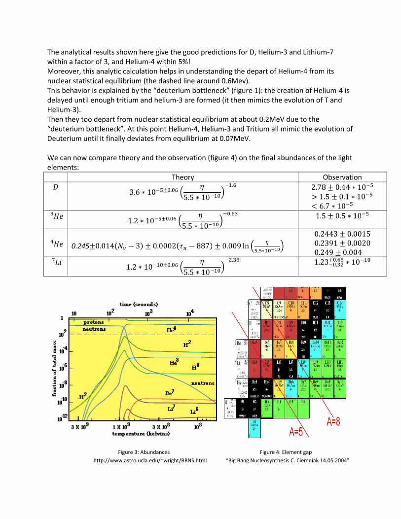
The analytical results shown here give the good predictions for D, Helium‐3 and Lithium‐7 within a factor of 3, and Helium‐4 within 5%! Moreover, this analytic calculation helps in understanding the depart of Helium‐4 from its nuclear statistical equilibrium (the dashed line around 0.6Mev). This behavior is explained by the “deuterium bottleneck” (figure 1): the creation of Helium‐4 is delayed until enough tritium and helium‐3 are formed (it then mimics the evolution of T and Helium‐3). Then they too depart from nuclear statistical equilibrium at about 0.2MeV due to the “deuterium bottleneck”. At this point Helium‐4, Helium‐3 and Tritium all mimic the evolution of Deuterium until it finally deviates from equilibrium at 0.07MeV.  We can now compare theory and the observation (figure 4) on the final abundances of the light elements: 

  Theory  Observation   3.6 10 .

5.5 10. 

2.78 0.44 101.5 0.1 106.7 10

  1.2 10 .5.5 10  

10  . 1.5 0.5

  

 

0.245 0.014 3 0.0002 887 0.009 ln.

  

0.00150.2391 0.0020 

04

0.2443

0.249 0.0  1.2 10 .

5.5 10.

 1.23 .

. 10   

 

 

      Figure 3: Abundances        Figure 4: Element gap                    http://www.astro.ucla.edu/~wright/BBNS.html            “Big Bang Nucleosynthesis C. Ciemniak 14.05.2004” 

d) Uncertainties 

As nucleosynthesis involves many different reactions, there are many sources of uncertainty.  The major uncertainties in   are due to  

• The experimental uncertainty on the neutron lifetime. The current value is considered to be2 887 2 . A change of 2  in the neutron lifetime causes a change in Helium‐4 prediction of about 0.4%.  

• The number of neutrino generations ; if the number of generations is more than 3, say 3.3 (as we will this that seems to be the current bound on the number of neutrino generations) then we get a change of about 1.5% in the abundance prediction. 

 For the other elements, uncertainties in the nuclear cross sections can dramatically modify the abundance predictions. They can alter D and   by up to 15% and   by about 50%! And all of this being a “chain reaction” a change in the reaction rate of one element will affect all the others. These effects can be neglected for the Helium‐4 abundance ( 0.3%) because as we have seen it is possible to calculate its abundance only using the neutron’s abundance at nucleation time; 

already got  very precis

Big  an  nucleosynthesis also allows to calculate the baryon to photon ratio .  

1.75 10  e, 

ced Hubble to put constraints on other observables like the 

we did not have to consider any of the nuclear reactions to do this calculations and a e result.  

B gFrom spectroscopic measurements, and taking 3, one gets the following value: 

5.15Which corresponds to ΩBh 0.018 0.006 where ΩB is the baryonic content of the universand   the redu  constant. As we will see later those parameters allow usnumber of neutrinos generations, their masses, but also to test the value of the fundamental 

constants like G and the fine structure constant  (constraint given by BBN is Δαα

5%.) 

 Big Bang nucleosynthesis is therefore a test for the hot Big Bang model, nuclear physics, and 

                                                           

astrophysics in general.           

 2 Particle Data Group 

Constraints 

to n rate of e niverse, therefore more neutrons will survive until nucleosynthesis which leads to an increase 

Number of Neutrino Flavors 

Model predictions for He‐4 

on new physics 

a) Number of neutrino generations 

An increase in the number of neutrino   leads   an increase in the expansio  thuin the Helium‐4 abundance. 

2 ~ 0.2273 ~ 0.2424 ~ 0.254

 Constraints from Big Bang nucleosynthesis are still very difficult to estimate (many different 

alues can be found in the literature). It seems like the best fit  ~3 0.3v . 

 

        Credits : arXiv:astro‐ph/9706069 

 

 

 

b) Neutrino masses 

Although in the “naïve” version of the Standard Model neutrinos are massless, recent experiments have tended to show that neutrinos were actually massive (from neutrino oscillation experiments mainly3). 

Even though their mass is thought to be extremely small, the large quantity of neutrinos implies that any non‐zero mass have an observable impact on cosmology. 

From nucleosynthesis, we can get an upper limit to the mass of all the neutrinos, by combining the relic neutrino abundance with observational bounds on present energy density (thanks to WMAP): 

2 94  

summing over all neutrino species that are relativistic at decoupling (i.e.   1 ). 

If we consider that neutrinos are more massive and therefore where not relativistic (!), then tic decoupling, the we get a lower limit 

on their mass:  2 . 

Therefore no stable neutrino can have a mass in the 100eV to 2GeV range. urrent neutrino mass estimations are: 

, 160 , 24  

n region. 

Ω  

ΩB

they fall out of chemical equilibrium before the relativis

C

2.1That is for now, only the electron‐neutrino is known to have a mass out of the forbidde

c) Dark matter 

Direct observations of luminous matter give the following result toward the content of the universe: 

h ~ 0.005

Comparing this to the previous value of ΩBh , we quickly understand that there is a problem : Ω

n 

30% ! Where are the other 70%?  

• Baryonic => no nucleonic dark matter, planetary mass black holes, “strange quark nuggets” (should have enhanced production of heavy elements during BBN). 

                                                           

• Non‐baryonic => Relic particles? New particles?  

 3 Super‐Kamiokande, 1998 

Conclusion 

For a long time, primordial nucleosynthesis and spectroscopic measurements where the only way to predict and test the light elements abundances, and to get a value for the baryonic content of the 

B) have allowed to c content of the universe: 

Ω h 0.0224 0.0009 which corresponds to a baryon to photon ratio : 

universe. However recent calculations4 of the Cosmic Microwave Background (CMmeasure with extreme accuracy the baryoni

6.14 0.25 10   If we redo all the previous calculations with those values, we get the following abundances: 

prediction using CMB values 

Element  Theoretical 

  2.60 0.170.19 10

  1.04 0.04 10 5 0.04

  0.247 0.0004   4.15 0.45

0.49 10 10  

photon ratio.  

The vertical line represents WMAP 

 The curves are the BBN predictions. 

Uzan & Peter 

On this graph are shown the theoretical predictions for 

Deuterium, Helium‐3, Helium‐4 and Lithium‐7 with respect to the baryon 

value for , the horizontal ones indicate the spectroscopic 

measurements for each element, the width representing the uncertainties.

Credits : “Cosmologie Pirmordiale” 

Tho  are in  theoretical predictions. Nuclear reaction rates are being reanalyzed because, , a slight change in one of them could greatly affect all the predictions. 

                                                           

se results conflict with the  as we have seen

 4 WMAP results on the CMB 

References 

Books 

“Cosmologie Primordiale” – Jean Philippe Uzan & Patrick Peter 

“Princ ” P.J.E Peebles iples of physical cosmology

ArXiV 

Xiv:astro‐ph/9706069 : Big‐bang Nucle

astro‐ph/0009506 : Light Elem

arXiv:astro‐ph/9905211 : Primordial Lithiu

rXiv:astro‐ph/0008495 : What Is The BBN

rXiv:astro‐ph/9905320 : Primordial Nucl

arXiv:hep‐ph/9602260 : Big Bang nucleosynthesis and physics beyond the Standard Model 

ar osynthesis Enters the Precision Era 

arXiv: ent Nucleosynthesis 

m and Big Bang Nucleosynthesis 

a  Prediction for the Baryon Density and How Reliable Is It? 

a eosynthesis: Theory and Observations 

Other Internet resources 

http://www.astro.ucla.edu/~wright/BBNS.html http://www‐thphys.physics.ox.ac.uk/users/SubirSarkar/mytalks/groningen05.pdf http://www.astro.uu.se/~bg/cosmology http://www.mpia.de/homes/rix/BBN_Lect.pdf 

rodden and Sean Carroll “TASI Lectures: Introduction to Cosmology” 

.pdf 

Mark T