berry-esseen bounds for general nonlinear statistics, with...
TRANSCRIPT

Berry-Esseen bounds for general nonlinearstatistics, with applications to Pearson’s and
non-central Student’s and Hotelling’s
Iosif Pinelis1,2 and Raymond Molzon1
1Department of Mathematical SciencesMichigan Technological University
2Supported in part by NSF grant DMS-0805946
September 18, 2011

Main results
Supporting and/or related results
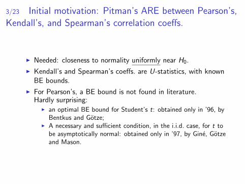
3/23 Initial motivation: Pitman’s ARE between Pearson’s,Kendall’s, and Spearman’s correlation coeffs.
I Needed: closeness to normality uniformly near H0.
I Kendall’s and Spearman’s coeffs. are U-statistics, with knownBE bounds.
I For Pearson’s, a BE bound is not found in literature.Hardly surprising:
I an optimal BE bound for Student’s t: obtained only in ’96, byBentkus and Gotze;
I A necessary and sufficient condition, in the i.i.d. case, for t tobe asymptotically normal: obtained only in ’97, by Gine, Gotzeand Mason.
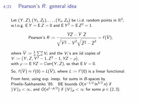
4/23 Pearson’s R : general idea
Let (Y ,Z ), (Y1,Z1), . . . , (Yn,Zn) be i.i.d. random points in R2;w.l.o.g. EY = EZ = 0 and EY 2 = EZ 2 = 1.
Pearson’s R :=YZ − Y Z√
Y 2 − Y2√
Z 2 − Z2
= f (V ),
where V := 1n
∑n1 Vi and the Vi ’s are iid copies of
V :=(Y ,Z ,Y 2 − 1,Z 2 − 1,YZ − ρ
),
with ρ := EYZ = Corr(Y ,Z ), so that EV = 0.
So, f (V ) ≈ f (0) + L(V ), where L := f ′(0) is a linear functional.
From here, using exp. ineqs. for sums in B-spaces byPinelis–Sakhanenko ’85: BE bounds O(n−1/2 ln3/2 n) if‖V ‖3 <∞, and O(n1−p/2) if ‖V ‖p <∞ for some p ∈ (2, 3).
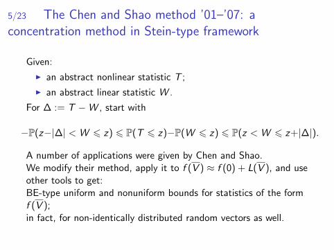
5/23 The Chen and Shao method ’01–’07: aconcentration method in Stein-type framework
Given:
I an abstract nonlinear statistic T ;
I an abstract linear statistic W .
For ∆ := T −W , start with
−P(z−|∆| <W 6 z) 6 P(T 6 z)−P(W 6 z) 6 P(z <W 6 z+|∆|).
A number of applications were given by Chen and Shao.We modify their method, apply it to f (V ) ≈ f (0) + L(V ), and useother tools to get:BE-type uniform and nonuniform bounds for statistics of the formf (V );in fact, for non-identically distributed random vectors as well.
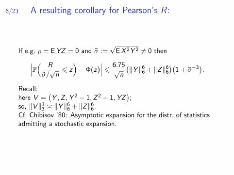
6/23 A resulting corollary for Pearson’s R :
If e.g. ρ = EYZ = 0 and σ :=√
EX 2Y 2 6= 0 then∣∣∣P( R
σ/√n6 z)− Φ(z)
∣∣∣ 6 6.75√n
(‖Y ‖66 + ‖Z‖66
)(1 + σ−3
).
Recall:here V =
(Y ,Z ,Y 2 − 1,Z 2 − 1,YZ
);
so, ‖V ‖33 � ‖Y ‖66 + ‖Z‖66.Cf. Chibisov ’80: Asymptotic expansion for the distr. of statisticsadmitting a stochastic expansion.
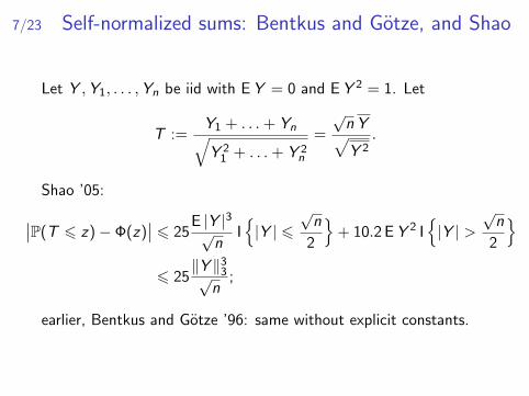
7/23 Self-normalized sums: Bentkus and Gotze, and Shao
Let Y ,Y1, . . . ,Yn be iid with EY = 0 and EY 2 = 1. Let
T :=Y1 + . . .+ Yn√Y 21 + . . .+ Y 2
n
=
√n Y√Y 2
.
Shao ’05:∣∣P(T 6 z)− Φ(z)∣∣ 6 25
E |Y |3√n
I{|Y | 6
√n
2
}+ 10.2 EY 2 I
{|Y | >
√n
2
}6 25
‖Y ‖33√n
;
earlier, Bentkus and Gotze ’96: same without explicit constants.
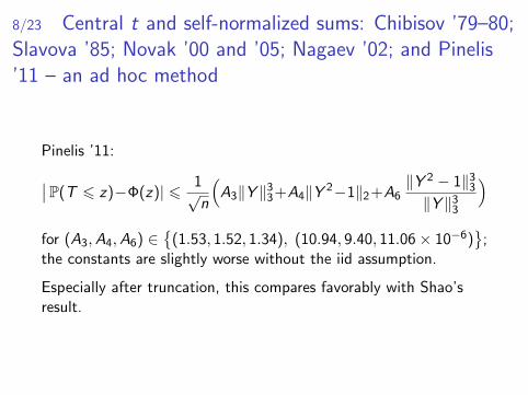
8/23 Central t and self-normalized sums: Chibisov ’79–80;Slavova ’85; Novak ’00 and ’05; Nagaev ’02; and Pinelis’11 – an ad hoc method
Pinelis ’11:∣∣P(T 6 z)−Φ(z)| 6 1√n
(A3‖Y ‖33+A4‖Y 2−1‖2+A6
‖Y 2 − 1‖33‖Y ‖33
)for (A3,A4,A6) ∈
{(1.53, 1.52, 1.34), (10.94, 9.40, 11.06× 10⁻⁶)
};
the constants are slightly worse without the iid assumption.
Especially after truncation, this compares favorably with Shao’sresult.
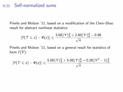
9/23 Self-normalized sums
Pinelis and Molzon ’11, based on a modification of the Chen–Shaoresult for abstract nonlinear statistics:∣∣P(T 6 z)− Φ(z)
∣∣ 6 3.68‖Y ‖33 + 2.60‖Y ‖44 − 0.98√n
.
Pinelis and Molzon ’11, based on a general result for statistics ofform f (V ):
∣∣P(T 6 z)− Φ(z)∣∣ 6 5.08‖Y ‖33 + 5.08‖Y ‖64 + 0.26‖Y 2 − 1‖33√
n.
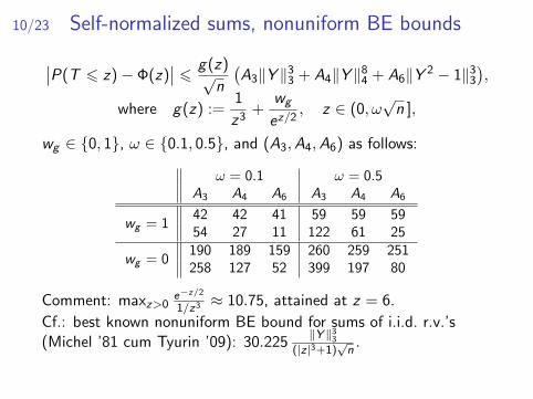
10/23 Self-normalized sums, nonuniform BE bounds
∣∣P(T 6 z)− Φ(z)∣∣ 6 g(z)√
n
(A3‖Y ‖33 + A4‖Y ‖84 + A6‖Y 2 − 1‖33
),
where g(z) :=1
z3+
wg
ez/2, z ∈ (0, ω
√n ],
wg ∈ {0, 1}, ω ∈ {0.1, 0.5}, and (A3,A4,A6) as follows:
ω = 0.1 ω = 0.5A3 A4 A6 A3 A4 A6
wg = 142 42 41 59 59 5954 27 11 122 61 25
wg = 0190 189 159 260 259 251258 127 52 399 197 80
Comment: maxz>0e−z/2
1/z3≈ 10.75, attained at z = 6.
Cf.: best known nonuniform BE bound for sums of i.i.d. r.v.’s(Michel ’81 cum Tyurin ’09): 30.225
‖Y ‖33(|z|3+1)
√n.

11/23 Self-normalized sums vs. Student’s statistic
For all n > 1∣∣∣∣ supz∈R
∣∣P(t 6 z)− Φ(z)∣∣− sup
z∈R
∣∣P(T 6 z)− Φ(z)∣∣∣∣∣∣ < C
n − 1,
where t is the Student statistic, T is again the self-normalized sum,
C :=(k − 1
2
)e−k
√k
π= 0.162 . . . , and k := 1 +
√3
2.
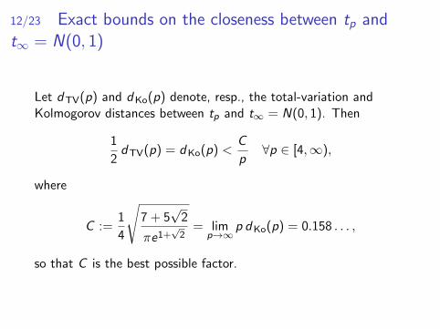
12/23 Exact bounds on the closeness between tp andt∞ = N(0, 1)
Let dTV(p) and dKo(p) denote, resp., the total-variation andKolmogorov distances between tp and t∞ = N(0, 1). Then
1
2dTV(p) = dKo(p) <
C
p∀p ∈ [4,∞),
where
C :=1
4
√7 + 5
√2
πe1+√2
= limp→∞
p dKo(p) = 0.158 . . . ,
so that C is the best possible factor.
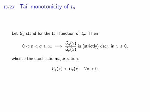
13/23 Tail monotonicity of tp
Let Gp stand for the tail function of tp. Then
0 < p < q 6∞ =⇒ Gq(x)
Gp(x)is (strictly) decr. in x > 0,
whence the stochastic majorization:
Gq(x) < Gp(x) ∀x > 0.

14/23 Exact upper bounds on the mean of theWinsorised-tilted distribution
For each h > 0 and each w ∈ R, the maximum of the tilted mean
EXeh(X∧w)
E eh(X∧w)
given EX and EX 2 is attained when X has a two-pointdistribution.
For EX = 0 and w > 0, this maximum is
<ehw − 1
wEX 2,
and the factor ehw−1w is the best possible.
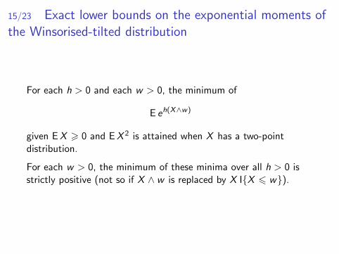
15/23 Exact lower bounds on the exponential moments ofthe Winsorised-tilted distribution
For each h > 0 and each w > 0, the minimum of
E eh(X∧w)
given EX > 0 and EX 2 is attained when X has a two-pointdistribution.
For each w > 0, the minimum of these minima over all h > 0 isstrictly positive (not so if X ∧ w is replaced by X I{X 6 w}).

16/23 An asymptotically Gaussian bound on theRademacher tails
P(a1ε1 + · · ·+ anεn > x) 6 P(Z > x) +Cϕ(x)
9 + x2
< P(Z > x)(
1 +C
x
)∀x > 0,
where ε1, . . . , εn are independent Rademacher r.v.’s,
a21 + · · ·+ a2n = 1,
Z ∼ N(0, 1) with density ϕ, andC := 5
√2πe P(|Z | < 1) = 14.10 . . . is a best possible constant
factor: the 1st inequality above turns into the equality whenx = n = 1.
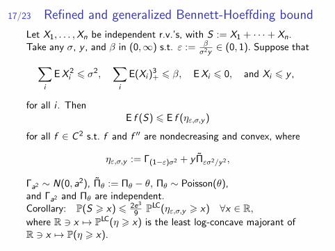
17/23 Refined and generalized Bennett-Hoeffding bound
Let X1, . . . ,Xn be independent r.v.’s, with S := X1 + · · ·+ Xn.Take any σ, y , and β in (0,∞) s.t. ε := β
σ2y∈ (0, 1). Suppose that∑
i
EX 2i 6 σ2,
∑i
E(Xi )3+ 6 β, EXi 6 0, and Xi 6 y ,
for all i . ThenE f (S) 6 E f (ηε,σ,y )
for all f ∈ C 2 s.t. f and f ′′ are nondecreasing and convex, where
ηε,σ,y := Γ(1−ε)σ2 + y Πεσ2/y2 ,
Γa2 ∼ N(0, a2), Πθ := Πθ − θ, Πθ ∼ Poisson(θ),and Γa2 and Πθ are independent.Corollary: P(S > x) 6 2e3
9 PLC(ηε,σ,y > x) ∀x ∈ R,where R 3 x 7→ PLC(η > x) is the least log-concave majorant ofR 3 x 7→ P(η > x).
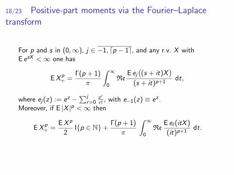
18/23 Positive-part moments via the Fourier–Laplacetransform
For p and s in (0,∞), j ∈ −1, dp − 1e, and any r.v. X withE esX <∞ one has
EX p+ =
Γ(p + 1)
π
∫ ∞0
ReE ej((s + it)X
)(s + it)p+1
dt,
where ej(z) := ez −∑j
r=0z r
r ! , with e−1(z) ≡ ez .Moreover, if E |X |p <∞ then
EX p+ =
EX p
2I{p ∈ N}+
Γ(p + 1)
π
∫ ∞0
ReE e`(itX )
(it)p+1dt.
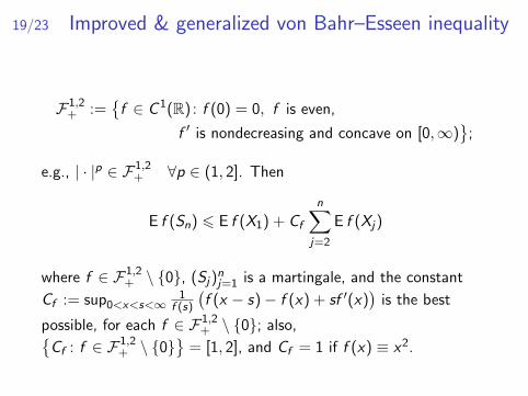
19/23 Improved & generalized von Bahr–Esseen inequality
F1,2+ :=
{f ∈ C 1(R) : f (0) = 0, f is even,
f ′ is nondecreasing and concave on [0,∞)}
;
e.g., | · |p ∈ F1,2+ ∀p ∈ (1, 2]. Then
E f (Sn) 6 E f (X1) + Cf
n∑j=2
E f (Xj)
where f ∈ F1,2+ \ {0}, (Sj)
nj=1 is a martingale, and the constant
Cf := sup0<x<s<∞1
f (s)
(f (x − s)− f (x) + sf ′(x)
)is the best
possible, for each f ∈ F1,2+ \ {0}; also,{
Cf : f ∈ F1,2+ \ {0}
}= [1, 2], and Cf = 1 if f (x) ≡ x2.

20/23 Corollary: concentration of measure for separatelyLipshitz (sep-Lip) functions
Let X1, . . . ,Xn be independent r.v.’s with values in X1, . . . ,Xn,resp.; here, all spaces and functions are measurable. Suppose
Y := g(X1, . . . ,Xn)
and the sep-Lip condition
|E g(x1, . . . , xi−1, xi ,Xi+1, . . . ,Xn)
−E g(x1, . . . , xi−1, xi ,Xi+1, . . . ,Xn)| 6 ρi (xi , xi )
holds for some functions ρi : Xi × Xi → R and all i , xj ∈ Xj , andxi ∈ Xi .(The sep-Lip condition is easier to check and more generally
applicable than joint-Lip. On the other hand, when joint-Lip holds,generally better bounds can be obtained.
)
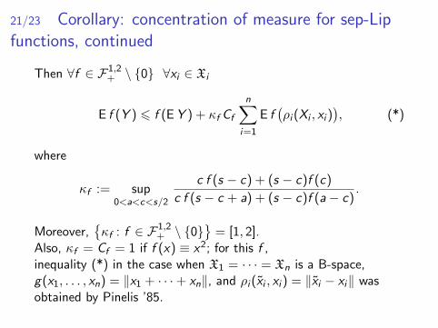
21/23 Corollary: concentration of measure for sep-Lipfunctions, continued
Then ∀f ∈ F1,2+ \ {0} ∀xi ∈ Xi
E f (Y ) 6 f (EY ) + κf Cf
n∑i=1
E f(ρi (Xi , xi )
), (*)
where
κf := sup0<a<c<s/2
c f (s − c) + (s − c)f (c)
c f (s − c + a) + (s − c)f (a− c).
Moreover,{κf : f ∈ F1,2
+ \ {0}}
= [1, 2].Also, κf = Cf = 1 if f (x) ≡ x2; for this f ,inequality (*) in the case when X1 = · · · = Xn is a B-space,g(x1, . . . , xn) = ‖x1 + · · ·+ xn‖, and ρi (xi , xi ) = ‖xi − xi‖ wasobtained by Pinelis ’85.
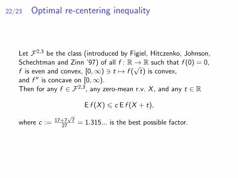
22/23 Optimal re-centering inequality
Let F2,3 be the class (introduced by Figiel, Hitczenko, Johnson,Schechtman and Zinn ’97) of all f : R→ R such that f (0) = 0,f is even and convex, [0,∞) 3 t 7→ f (
√t) is convex,
and f ′′ is concave on [0,∞).Then for any f ∈ F2,3, any zero-mean r.v. X , and any t ∈ R
E f (X ) 6 c E f (X + t),
where c := 17+7√7
27 = 1.315... is the best possible factor.

23/23
Thank you!