benefits to processor load for quadrature baseband versus radio

Benefits to Processor Load for Quadrature

Baseband versus Radio Frequency Demodulation

Algorithms

LUSUNGU NDOVI

Thesis presented in partial fulfilment of the requirements for the degree of

Master of Science in Electronic Engineering

At Stellenbosch University

SUPERVISOR: Prof. J.G. LOURENS

Co-SUPERVISOR: Dr. R. WOLHUTER

December 2008

Declaration By submitting this thesis electronically, I declare that the entirety of the work contained

therein is my own, original work, that I am the owner of the copyright thereof (unless to

the extent explicitly otherwise stated) and that I have not previously in its entirety or in

part submitted it for obtaining any qualification.

Date: December 2008

Copyright © 2008 Stellenbosch University

All rights reserved

i

Abstract Keywords: Quadrature baseband, QBB, Radio frequency, RF, Beamforming,

Multipath compensation, Doppler shift compensation, Software-defined radio, SDR,

Matched filter detection.

The continued advancement and improvement of software-defined radio technology has

been a key factor in furthering research into the implementation of most signal

processing algorithms at baseband. Traditionally, these algorithms have been carried

out at RF, but with the coming of SDR, there has been a need to shift the processing

down to baseband frequencies which are more compatible with the fast developing

software radio technology.

The study looks at selected demodulation algorithms and investigates the

possibility and benefits of carrying them out at QBB. The study ventures into the area

of beamforming, multipath compensation, Doppler shift compensation and matched

filter detection. The analysis is carried out using Matlab simulations at RF and QBB.

The results obtained are compared, not only to evaluate the possibility but also the

benefits in terms of the processing load. The results of the study showed that indeed,

carrying out the selected demodulation algorithms at QBB was not only possible, but

also resulted in an improvement in the processing speed brought about by the reduction

in the processing load.

ii

Opsomming Kernwoorde: Kwadratuur basisband, QBB, Radiofrekwensie, RF, Bundelvorming

Multi-pad kompensasie, Dopplerskuif kompensasie, Sagteware gedefineerde radio,

SDR, aangepaste filter deteksie.

Die aangaande vooruitgang en verbetering in sagteware gedefineerde radio tegnologie

was ‘n groot faktor om die implementasie van meeste sein verwerkings algoritmes by

basisband verder na te vors. Tradisioneel, was hierdie algoritmes by RF gedoen, maar

met die ontwikkeling van SDR was daar 'n behoefte om die verwerking by basisband te

doen wat meer versoenbaar is met vinnige groeiende sagteware radio tegnologie

Die studie kyk na geselekteerde demodulasie algoritmes en ondersoek die

moontlikheid en voordele daarvan om dit by QBB uit te voer. Die studie kyk verder na

bundelvorming, multi-pad kompensasie, Doppler skuif en aangepaste filters deteksie.

Die analise word uitgevoer deur van Matlab implementasies gebruik te maak by RF en

QBB. Die resultate word vergelyk om nie net die moontlikheid nie, maar ook die

voordele in terme van verwerkingslas te ordersoek. Die resultate van die studie het

gewys dat die demodulasie algoritmes by QBB nie net moontlik is nie, maar ook’ n die

verbetering in prossesserings-spoed veroorsaak het, deur die verwerkingslas te

verminder.

iii

Acknowledgements

I would like to thank the following:

• My supervisor, Prof Johan Lourens for his support, supervision and guidance

during the whole course of my studies.

• My co-supervisor Dr Riaan Wolhuter for his support, supervision and guidance

in finalising my studies.

• Dr G-J van Rooyen for his support.

• My friends and colleagues in the DSP lab.

• The Copperbelt University (CBU) in Zambia for their financial support.

• My mom and sisters Suzyo and Lushomo for their encouragement.

• Above all GOD the creator.

iv

Contents

Nomenclature

1 INTRODUCTION

1.1 Motivation………………………………………………………….….

1.2 Objectives……………………………………………………………...

1.3 Thesis overview………………………………………………...……...

2 BACKGROUND THEORY

2.1 Software defined radio and baseband processing……………………..

2.2 Quadrature baseband………………………………………………….

2.3 Beamforming……………………………………………………….....

2.3.1 Beamforming at RF…………………………………………………...

2.3.2 Beamforming at QBB…………………………………………………

2.4 Multipath………………………………………………………………

2.4.1 Spectral changes due to time shift in a signal……………….….....

2.4.2 RF and QBB multipath compensation…..……..…………………...

2.5 Doppler shift………………………………...…………………………

2.6 Multiple compensation……….………………………………………..

2.7 Matched filtering:- Chirp signal………………………………….........

2.8 AMDSB-SC, AMDSB-LC, FM and QAM……………………………

2.8.1 AMDSB-SC.................................................................................

2.8.2 AMDSB-LC..……………………………………………..…….

2.8.3 FM ………………………….……..................................................

2.8.4 QAM (analogue)………….…….…………………..…………..…...

2.9 Channel/Compensator reciprocity………...………..………...................

2.10 Benefits of working at QBB…………………………….………………

2.11 Conclusion………………...……………….…………………..………..

3 BEAMFORMING SIMULATION RESULTS

3.1 RF Beamforming……………………………..……………………….

3.2 QBB Beamforming……………………………………..……………..

xiii

1

1

1

1

5

5

5

9

10

10

12

12

13

14

14

15

17

17

18

19

19

20

21

21

22

22

24

v

3.3 MatLab simulation results AMDSB-SC………..………..…………....

3.4 Simulation results:-QBB Beamforming………………………………..

3.5 Beam patterns comparisons…………………………………………….

3.6 MatLab simulation results AMDSB-LC……………………………….

3.6.1 Beamforming AMDSB-LC……………………….…………………..

3.6.2 Coherent and Non-Coherent methods………………..…………….

3.6.2.1 Coherent detection………………..…............................

3.6.2.2 Envelope detection…………………….………………

3.6.4 Simulation results:- QBB……………………………………...……..

3.6.5 Beam pattern comparisons……………………………………....

3.7 MatLab simulation results:-FM………………………………...............

3.7.1 Simulation results:-beamforming at RF……………………….......

3.7.2 Simulation results:-beamforming at QBB ………………............

3.7.3 Numerical comparison of beam patterns ......……………….….

3.8 Benefits of beamforming at QBB……………………….……………..

3.8.1 Sampling frequency and bandwidth……………….………………

3.8.2 Sample processing and simulation time……..…………..……….

3.9 Conclusion………...……………………………………………………

4 MULTIPATH COMPENSATION:- SIMULATION RESULTS

4.1 Multipath compensation.……………………………………………….

4.2 Multipath compensation:- RF………………………………………......

4.3 Multipath compensation:-QBB……...………………………………….

4.4 Simulation results QAM RF compensation...…………………………..

4.5 Simulation results QAM QBB compensation………………………….

4.6 Simulation results FM RF compensation……………………………....

4.7 Simulation results FM QBB compensation results.…………………….

4.8 Benefits of multipath compensation at QBB…...…………………...….

4.9 Conclusion………….……………………………………………...…...

27

28

29

31

31

31

32

33

33

39

39

39

41

42

43

43

45

48

49

49

51

54

57

60

63

66

67

70

vi

5 DOPPLER SHIFT COMPENSATION:- SIMULATION RESULTS

5.1 Doppler shift……………………………………...…………………..

5.2 Doppler shift model signal modelling……...………………………...

5.3 Theoretical analysis:- Compensation at RF…………………………..

5.4 Theoretical analysis:- Compensation at QBB…..……………………

5.5 Simulation:- QAM RF compensation…………….....………………..

5.6 Simulation:- QAM QBB compensation…………...………….……...

5.7 Simulation results:-FM Doppler shift compensation at RF…………..

5.8 Simulation results:-FM Doppler shift compensation at QBB………..

5.9 Benefits of compensating for Doppler shift at QBB…………………

5.10 Conclusion……………………………………………………………

6 MULTIPLE COMPENSATION:- SIMULATION RESULTS

6.1 Signal modelling………….…………………………………………..

6.2 Special case…………………………………………………………..

6.3 Simulation results……………..……………………………………...

6.4 Special case simulation results RF…………………………………...

6.5 Special case simulation results QBB……………….………………...

6.6 Benefits of multiple compensation at QBB….…………………….....

6.7 Conclusion……………………………………………………………

7 MATCHED FILTER DETECTION:- SIMULATION RESULTS

7.1 Matched filter detection………………………...…………………….

7.2 Matched filter detection:-noiseless channels………………………....

7.2.1 Theoretical analysis:- RF………...............................................

7.2.2 Theoretical analysis:- QBB…..………………………………..

7.3 MatLab simulation results:- RF and QBB………….....…...…………

7.3.1 RF:- direct path………………….………………....................

7.3.2 QBB:- direct path………..…………..………………………..

7.4 RF multipath……………….....……………….……………………...

7.5 QBB multipath……………………….....……………...…………….

7.6 RF Doppler shift…..…………..……....……………….…...………...

71

71

72

72

75

77

81

84

85

86

88

89

89

92

93

95

97

99

101

102

102

103

103

104

105

105

107

108

110

112

vii

7.7 QBB Doppler shift..…………………..……….....……………………

7.8 Multiple signal input: RF……………….…………………………..…

7.9 Multiple signal input: QBB……………….………………..……..….

7.10 Matched filter detection:- noisy channels…………………………......

7.10.1 Matched filter detection:- RF…………………………….......

7.10.2 Simulation results:-RF……………………………………….

7.10.3 Matched filter detection:- QBB.……………..……………….

7.10.4 Simulation results:-QBB….…………………………...……..

7.11 Matched filter detection: Multiple signal input at RF and QBB...........

7.11.1 Simulation results:-RF…………………………………..........

7.11.2 Simulation results:-QBB………………………………..…….

7.12 Benefits of matched filter detection at QBB…………………..………

7.13 Conclusion…………………………………………………….............

8 CONCLUSIONS

8.1 Conclusion…………………………………………………………….

8.2 Summary of overall results……………………………………………

8.3 Future work…….…………….………………………………………..

BIBLIOGRAPHY M FILES CREATED

APPENDIX A Probability of error derivation theoretical derivation.……..…... APPENDIX B Model of slowly fluctuating target……………………….…….. APPENDIX C Matlab source code CD ……………………………………….

113

115

117

119

121

122

123

124

125

128

129

132

133

134

134

135

136

137

140

142

145

147

viii

List of Figures 2.1 Comparison of baseband and radio frequency version of an AM signal…… 2.2 Conversion of an RF signal to QBB………………………………...……… 2.3 Spectral changes from RF to QBB………………………………………..... 2.4 Analogue down-mixing and QBB generation……………………………… 2.5 Channel impulse response………………………………………………….. 2.6 Matched filter detection flow diagrams (RF and QBB)……………………. 2.7 QBB DSB-SC demodulation block diagram……………………………….. 2.8 QAM QBB demodulation………………………………………………….. 2.9 Channel/Compensator reciprocity structure………………………………... 3.1 RF beamforming theoretical analysis block diagram……………………..... 3.2 QBB beamforming theoretical analysis block diagram…………………...... 3.3 Simulation results RF beamforming for AMDSB-SC……………………… 3.4 Beam pattern QBB beamforming…………………………………………... 3.5 Beam pattern comparisons………………………………………………….. 3.6 Difference plots…………………………………………………………….. 3.7 AMDSB-LC beamforming RF beamforming flow diagram………….…..... 3.8 MatLab code structure coherent detection………………………………...... 3.9 Simulation results RF beamforming:-coherent detection…………………... 3.10 Beam pattern:-coherent detection…………………………………….…...... 3.11 MatLab code structure:-Envelope detection……………………………....... 3.12 Simulation results AMDSB-LC Envelope detection……………………….. 3.13 Beam pattern:-Envelope detection………………………………………...... 3.14 MatLab code structure QBB AMDSB-LC beamforming…………………... 3.15 Simulation results AMDSB-LC QBB AMDSB-LC………………………... 3.16 MatLab comparison structure and difference plots………………………… 3.17 Simulation results beamforming FM:-QBB………………………………... 3.18 Simulation results beamforming FM:-QBB………………………………... 3.19 MatLab comparison structure and difference plot………………………….. 3.20 RF/QBB sampling frequency comparison………………………………….. 4.1 Multipath signal reception model………………………………................... 4.2 RF multipath compensation theoretical analysis flow diagram…………..… 4.3 QBB multipath compensation theoretical analysis flow diagram……..…… 4.4 Simulation results QAM RF multipath compensation……………..……..... 4.5 Simulation results:-demodulated signals and error plot…………………..... 4.6 Magnitude spectral plots RF multipath compensation…………………....... 4.7 Magnitude spectrum of compensated signal…………………………..…… 4.8 Channel impulse response…………………………………………..…..….. 4.9 Simulation results QBB……………………………………………….......... 4.10 Simulation results QBB continued……………………………………….....

6 7 8 11 13 16 17 20 21 23 26 27 29 30 30 32 33 34 35 35 36 37 37 38 39 40 41 42 43 49 52 55 57 58 59 59 60 61 61

ix

4.11 Simulation results QBB demodulated signal and error plot………………. 4.12 Spectral changes QBB………………………………………..…………… 4.13 Simulation results FM RF multipath compensation……………………..... 4.14 Demodulated output and difference plot………………………………...... 4.15 Simulation results FM QBB multipath compensation…………………...... 4.16 Difference plot…………………………………………………..………… 5.1 Doppler shift model……………………………………………………...... 5.2 Theoretical analysis at RF………………………………………………… 5.3 Theoretical analysis at QBB……………………………………………..... 5.4 Simulation results QAM RF……………………………………………..... 5.5 Simulation results QAM RF continued…………………………………… 5.6 Spectral plots QAM RF…………………………………………..……….. 5.7 Spectral plots QAM RF continued……………………………………....... 5.8 Spectral plots QAM RF continued………………………………………... 5.9 Simulation results QAM QBB…………………………………………...... 5.10 Demodulated output and difference plot………………………………...... 5.11 Spectral analysis QBB…………………………………………………...... 5.12 Simulation results FM RF continued……………………………………… 5.13 Simulation results FM QBB……………………………………………..... 5.14 Difference plot…………………………………………………………...... 6.1 Multiple signal reception model…………………………………………... 6.2 Received signal generation structure……………………………………… 6.3 Spectra of input signal for special case…………………………………… 6.4 Simulation results multiple compensation RF…………………………….. 6.5 Simulation results multiple compensation RF continued……………….… 6.6 Special case simulation results RF………………………………………... 6.7 Spectral plots for special case at RF………………………………………. 6.8 Compensated and demodulated outputs…………………………………... 6.9 Special case simulation results QBB……………………………………… 6.10 Compensated demodulated outputs and error plot………………………... 7.1 RF chirp analysis………………………………………………………….. 7.2 QBB chirp analysis………………………………………………………... 7.3 Simulation results:- RF direct path…………………………...…………… 7.4 Simulation results:- QBB direct path…………………..…………………. 7.5 RF multipath analysis model……………………………………………… 7.6 Simulation results:- RF multipath……………………………...………..... 7.7 QBB multipath analysis model……………………………………………. 7.8 Simulation results:- QBB multipath…………………………...………...... 7.9 RF Doppler shift analysis model………………………………………….. 7.10 Simulation results:- RF Doppler shift……………………...…………….... 7.11 QBB Doppler shift analysis model………………………………………... 7.12 Simulation results:- QBB Doppler shift………...…………………………

62 63 64 65 66 67 71 74 76 77 78 78 79 79 81 82 83 84 85 86 89 91 92 93 94 95 96 97 98 99 103 104 105 107 108 109 110 111 112 112 113 114

x

7.13 RF Multiple input analysis model………………………………………… 7.14 Simulation results:- RF Multiple input………….……………………....... 7.15 QBB Multiple input analysis model………………………………………. 7.16 Simulation results:- QBB Multiple input………………………...……….. 7.17 RF simulation flow:-direct path…………………………………………… 7.18 Simulation results:- RF direct path…………………………………...…… 7.19 QBB simulation flow:-direct path………………………………………… 7.20 Simulation results:- QBB direct path…..…………………………………. 7.21 RF theoretical analysis:-Multiple input…………………………………… 7.22 QBB theoretical analysis:-Multiple……………………..………………… 7.23 QBB simulation flow diagram:-Multiple input………….………………... 7.24 Simulation results RF:-Multiple input…...………………..……………..... 7.25 Probability of error plots:- RF Multiple input…………...………………... 7.26 Simulation results QBB:- Multiple input…………...…………………….. 7.27 Probability of error plots:- QBB Multiple input………...…………………

115 116 117 118 119 122 123 124 126 126 127 128 129 130 131

xi

List of Tables 3.1 Sample processing for AMDSB-SC simulation………………………..….

3.2 Simulation time and sample processing ratio summary………………..….

4.1 Sample processing for QAM simulation….……...………………….….…

4.2 Simulation time and sample processing ratio summary……………….…..

5.1 Sample processing for QAM simulation……………………………..……

5.2 Simulation time and sample processing ratio summary………………..….

6.1 Sample processing at for multiple signal input simulation………………..

6.2 Simulation time and sample processing ratio summary…………………...

7.1 Simulation time and sample processing ratio summary…………………....

8.1 Summary of overall simulation results……………………….………….....

46

47

68

69

87

88

100

100

132

135

xii

Nomenclature Acronyms AM Amplitude Modulation LSB Lower Sideband LO Local Oscillator RF Radio Frequency QBB Quadrature Baseband SDR Software Defined Radio AM DSB-SC Amplitude Modulated Double Side Band-Suppressed Carrier AM DSB-LC Amplitude Modulated Double Side Band-Large Carrier FM Frequency Modulation QAM Quadrature Amplitude Modulation LPF Low Pass Filter MIMO Multiple Input Multiple Output FFT Fast Fourier Transform DFT Discrete Fourier Transform IFFT Inverse Fourier Transform SDMA Space Division Multiple Access MAX Maximum DSP Digital Signal Processor I/Q In-phase and Quadrature Components MF Matched Filter

xiii

Variables Symbol Description

f(t) Modulating input for AM m(t) Modulated signal input for AM fc Carrier frequency fm Modulating signal frequency ω Instantaneous frequency ωc Carrier angular frequency ωm Modulating signal angular frequency θ Phase angle Ф Phase angle delay F(ω) General frequency domain signal λ Wave length c Speed of light dt Time delay t Continuous time T Discrete time period AF Antenna array factor f(ψ) Normalized array factor Pe Probability of error

1

Chapter 1

Introduction

1.1 Motivation

Modulation shifts a signal up to much higher frequencies than its original span. This

often results in doubling of the bandwidth. However, baseband frequencies are much

lower than radio frequencies and therefore, signal processing at baseband presents this

key advantage of working at much lower frequencies [2]. Processing at the lower QBB

enables more sub-sampling to take place than at RF and this in turn results in a

reduction in the number of samples being processed entailing a reduction in the

processor load and subsequently an improvement in processing speed. However, one

cannot substantiate the advantages of working at QBB without firstly carrying out the

study and then producing results that will justify the purpose of the research.

1.2 Objectives

The primary objective of the study was to investigate the possibility and benefits in

terms of processor load of carrying out beamforming, multipath compensation, Doppler

shift compensation, multiple compensation for multipath and Doppler shift, and

matched filter detection at quadrature baseband for selected modulation schemes. The

study showed the expected benefits of carrying out these techniques at quadrature

baseband and the advantages of QBB over RF were seen by comparing and discussing

the results from the RF and QBB simulations. Noiseless transmissions and narrowband

signals were assumed.

1.3 Thesis overview

The structure of the thesis is as follows:

Chapter 2: Background theory and literature review

This chapter outlines software defined radio and its development in relation to the

advancement of baseband processing. Quadrature baseband is explained and its

2

CHAPTER 1 - INTRODUCTION

role in the advancement of software radio technologies is also discussed. A general

general for the beamforming, multipath, Doppler shift, multiple compensation and

matched filter detection is given. The QBB demodulation of the modulation schemes

that were used in the simulations are summarised and the reciprocity that exists between

a channel and compensator is discussed. The mode of accessing the benefits in terms of

processor load and speed of QBB over RF implementation of the techniques and

demodulation algorithms under discussion is also given.

Chapter 3: Beamforming

This chapter investigates beamforming for AM DSB-SC, AM DSB-LC and FM

modulation schemes and simulation results obtained from the RF and QBB

beamforming are given and discussed. Firstly, the possibility of beamforming at QBB

is proved as well as the benefits and outcome of beamforming at QBB. The benefits of

working at QBB in terms of processor load will be seen in terms of simulation runtime

and number of calculations done for the simulations at RF and QBB. It should be noted

that the analogue and digital ways of generating QBB will be both considered in the

comparison process. It is shown from the results obtained that the processing load does

increase when beamforming at QBB as compared to RF for the simulation case in

which the QBB signals are generated digitally. However, when considering the real life

case in which the QBB signals are generated using analogue method, QBB emerged

more superior to RF in terms of processing load which in turn resulted in a reduction in

the processing time required.

Chapter 4: Multipath compensation

This part of the study investigated multipath compensation at RF and QBB for QAM

and FM modulation schemes. Similarly, the simulation results from the multipath

compensation analysis for the two modulation schemes are discussed and the benefits of

compensating at QBB compared to their RF counterparts. It is shown that the

compensation process is possible at QBB coupled with the expected benefits that come

along with doing so in terms of the processing time and load.

3

CHAPTER 1 - INTRODUCTION

Chapter 5: Doppler shift compensation

This chapter investigates Doppler shift compensation at RF and QBB for QAM and FM

modulation schemes. The simulation results from the Doppler shift compensation

analysis for the two modulation schemes are given and discussed. The possibility of

compensating for Doppler shift at QBB is shown and the benefits of working at QBB in

comparison to RF will be evaluated. Similarly, the simulation runtime and sample

processing results show why QBB is more advantageous than RF implementation of the

compensation process.

Chapter 6: Multiple signal compensation

The study in this chapter considers a special case where we have multiple inputs but

with a signal output. This part of the study investigates the possibility and benefits of

compensating for multipath and Doppler shift compensation at QBB as compared to RF

in the case of multiple signal reception. The simulation results are given, analysed and

discussed. The analysis considers QAM modulated signals. The chapter shows the

possibility of multiple compensation RF and QBB and if not, the reasons for the

simulation outcome are outlined and discussed. For the possible compensation

scenario, the benefits in terms of processing load and time of QBB against RF are

shown and reasons why it is more advantageous to work at QBB.

Chapter 7: Matched filter detection

The study moves to the digital processing arena by investigating matched filter

detection of a chirp signal at RF and QBB. It considers cases of the direct path,

multipath, Doppler shift and multiple signal input situation. The simulation results are

given and discussed as done for the previous chapters. The chapter firstly considers

noiseless transmissions and then considers two cases of noisy channel transmissions

with the matched filter detection taking place at RF and QBB. The processing load and

simulation run times are analysed for the noiseless and noisy transmission cases and the

results show that it is more advantageous in terms of processing load to carry out the

4

CHAPTER 1 – INTRODUCTION

matched filter detection process at QBB as compared to doing so at RF.

Chapter 8: Conclusion, M-Files

The study is concluded in this chapter and a summary of the findings from the study is

given and discussed. It will be interesting to see the variations in results obtained from

the various simulations carried out. The M-Files which were created are also given.

The study results show that carrying out the selected demodulation algorithms at

quadrature baseband is not only possible but does also result in an improvement in

processing speed caused by the reduction in processing load when sub-sampling is

carried out. Interesting results are seen for the beamforming case where the processor

load is more at QBB than at RF for the simulated QBB but when the real life analogue

down-mixed QBB case is considered, there is a much bigger reduction in the amount of

computation required at QBB.

5

Chapter 2

Background theory: Quadrature baseband,

beamforming, compensation and demodulation

algorithms

The chapter gives a background of the main components of the study. The concept of

quadrature baseband is explained in detail giving an insight into the reasons for carrying

out the study. The selected demodulation algorithms that were analysed in the study

are outlined and the general simulation flow structures are given so as to have a preview

of the actual simulation analysis to be carried out in later chapters. The mode of

measuring the simulation runtime and amount of computation so as to see the benefits

of working at quadrature baseband is explained.

2.1 Software defined radio and baseband processing Software radio technology advancement has been a factor in promoting research into

baseband signal processing. Baseband signal processing technology is experiencing a

period of radical change [16, 17]. This has prompted the need to investigate more about

baseband processing in order to implement most functions that were traditionally

implemented at RF so as to utilise the benefits that come with working at baseband.

2.2 Quadrature baseband

Quadrature baseband is a term that refers to the generation of in-phase and quadrature

components of a signal at baseband. Baseband is an adjective that describes signals

and systems whose range of frequencies is measured from 0 to a maximum bandwidth

or highest signal frequency [15]. Usually, it is considered as a synonym to lowpass and

an antonym to passband. The simplest definition is that a signal’s baseband bandwidth

is its bandwidth before modulation and multiplexing, or after demultiplexing and

demodulation. The figure on the next page illustrates the comparison between radio

frequency and baseband.

6

CHAPTER 2 – BACKGROUND THEORY

Power

Signal at basebandSignal at RF (radio fequency)

frequency0 fc

Figure 2.1: Comparison of the baseband version and RF version of an AM modulated

signal. The RF signal sits at the carrier frequency fc.

Quadrature baseband modulation/demodulation basically processes baseband signals

which is basically a signal having in-phase and quadrature phase components [1, 15].

Before undertaking the study in depth, it is necessary to define and distinguish clearly

the various components of software defined radio. These are defined below [6]:

- Baseband modulation:- refers to the generation of I and Q signals containing

modulated information (digital).

- Quadrature upmixing:- refers to the multiplication of the I(t) and Q(t) signals

with quadrature shifted carriers which are subtracted from each other to produce

the RF signal (analogue).

- Quadrature modulation:- refers to the combination of the baseband modulation

and quadrature upmixing and in its entirety represents the conversion from the

modulating to modulated signal.

- Baseband demodulation:- refers to the DSP method of recovering a modulated

signal from I and Q signals (digital).

- Quadrature downmixing:- refers to the multiplication of the received RF signal

(analogue) with quadrature shifted carriers resulting in two baseband signals I(t)

and Q(t).

- Quadrature demodulation:- refers to the combination of the baseband

demodulation and quadrature downmixing and in its entirety represents the

conversion from the modulated to the demodulated signal [6].

7


- Sampling:- refers to the conversion of analog signals into discrete impulses or

samples so as to be easily processed using digital technology.

The conversion of an RF signal to quadrature baseband is carried out by the following

steps:

• The RF signal is multiplied with a complex carrier in what is referred to as

down-mixing.

• The complex down-mixed signal is then lowpass filtered resulting in the

quadrature baseband version of the RF signal. The expressions given below

illustrate these steps.

Let ωc be the carrier frequency of the modulated RF signal, it follows that the complex

carrier used in the down-mixing process is a complex exponential with the same carrier

frequency ωc.

( ) ( ) cj tdownmixedf t f t e ω−= i (2.1)

The low pass filter then eliminates the high frequency component of the spectrum

resulting in the complex baseband signal.

( ) [ ( ) ]qbb downmixed LPFf t f t= (2.2)

The real part of the lowpass filtered signal corresponds to the inphase quadrature

component of the baseband signal [1]. The figure below illustrates the process outlined

above. The spectral changes resulting from the conversion from RF to baseband are

also shown in Figure 2.3 on the next page.

LPFXRF input QBB output

cj te ω−

down-mixed signal

Figure 2.2: Conversion of an RF carrier to quadrature baseband.

8


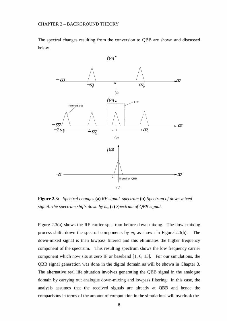
The spectral changes resulting from the conversion to QBB are shown and discussed

below.

( )f ω

ω

ω

ω

cω

( )f ω

( )f ω

0

0

0

Filtered out

Signal at QBB

(a)

(b)

(c)

LPF

cω−

cω−

cω2 cω−

ω−

ω−

ω−

Figure 2.3: Spectral changes (a) RF signal spectrum (b) Spectrum of down-mixed

signal:-the spectrum shifts down by ωc (c) Spectrum of QBB signal.

Figure 2.3(a) shows the RF carrier spectrum before down mixing. The down-mixing

process shifts down the spectral components by ωc as shown in Figure 2.3(b). The

down-mixed signal is then lowpass filtered and this eliminates the higher frequency

component of the spectrum. This resulting spectrum shows the low frequency carrier

component which now sits at zero IF or baseband [1, 6, 15]. For our simulations, the

QBB signal generation was done in the digital domain as will be shown in Chapter 3.

The alternative real life situation involves generating the QBB signal in the analogue

domain by carrying out analogue down-mixing and lowpass filtering. In this case, the

analysis assumes that the received signals are already at QBB and hence the

comparisons in terms of the amount of computation in the simulations will overlook the

9


down-mixing and lowpass filtering stage. Chapter 3 will gives more details about this

process.

2.3 Beamforming

Beamforming is a signal processing technique that is widely used to enhance signal

strength. It enables the reuse of the same carrier frequency by signals from other

directions. It also enhances antenna sensitivity so as to improve the signal to noise ratio

especially in the event of receiving weak signals [9]. Through beamforming, smart

antennas offer low co-channel interference and large antenna gain to the desired signals

which leads to more improved performance than conventional antenna systems.

Implementing beamforming in DSP enables arrays to benefit from a single steerable

antenna with a narrow gain pattern. SDR enables the beamforming to be performed

using software and hence formation of several beams is possible by simply reusing the

array output. This entails the possible usage of these software techniques in MIMO

systems. Smart antennas have brought about significant benefits to latest wireless

technologies [16]. The coming of software defined radio is a key advancement in

enabling smart antenna base stations to be realized by utilizing baseband beamforming

[16]. The study carries out beamforming at RF and QBB and compares the results.

Sections 2.3.1 and 2.3.2 outline beamforming at RF and QBB respectively.

The study will be carried out using MatLab analysis and then, comparisons will be

made between the beam patterns produced by the two beamforming methods. It

involves carrying out beamforming upon the reception of 4 input signals for each of the

modulation methods under investigation. The 4 input signals for both the RF and QBB

case are aligned at an angle theta `θ’ to the antenna array. The weighting coefficient of

the antennas was assumed to be unity for simplicity sake. The first signal has no input

delay whilst the other three signals have a delay `∆t’ determined by ‘θ’ and other

parameters. The analysis is to be done by varying ‘θ’ from 0 to 2π. Therefore, the

results of our analysis in MatLab will justify the possibility of carrying out

beamforming at quadrature baseband.

10


2.3.1 Beamforming at RF

Simple beamforming at RF involves summing up the 4 input signals at RF before

demodulating the summed-up signal. The beam pattern is produced from the output

signal by plotting the amplitude of the output signal against theta. The antenna

weighting coefficients are assumed to be equal to 1 for simplicity.

2.3.2 Beamforming at QBB

The procedure under QBB involves mixing down the incoming signals to quadrature

baseband. The beamforming process now takes place at QBB. The processing in an

SDR (real life case) assumes the processing of the signals already at QBB. Therefore,

comparisons will be made between the simulated QBB beamforming and the simulated

RF beamforming. The real life analogue down-mixed QBB scenario was considered for

merely showing the benefits of QBB over RF in terms of processing load and was thus

not simulated. In the chapters that follow, it will be interesting to see why working at

QBB is more beneficial in terms of the simulation runtime and the amount of numerical

processing as compared to RF. The main reason that will be seen that makes working

at QBB superior to RF in terms of processor load reduction is the fact that working at

QBB facilitates for further downsampling [32] to take place which inturn reduces the

number of samples being processed. Does this entail a definite reduction in the

simulation runtime too? The simulation results given in the next chapters will answer

this question since comparisons between the runtimes and number of calculations in the

simulation code at RF and QBB will be compared. Working at RF does have a

limitation in the downsampling process with aliasing more likely to occur resulting in

signal distortion. The analogue down-mixing process is illustrated in the Figure 2.4 on

the next page. In our simulations, the processing time was measured using inbuilt

MatLab commands and the amount of processing was depicted by the number of

numerical calculations taking place in the codes that executed the processes being

analyzed. It should be emphasised that the simulation runtime and numerical

processing measurements that were carried out in the study were carried out using

relative methods.

11


X

X LPF

LPF

DSP

sampling takesplace here

inphase carrier

Quadrature phase carrier

Received signal

I(t)

Q(t)

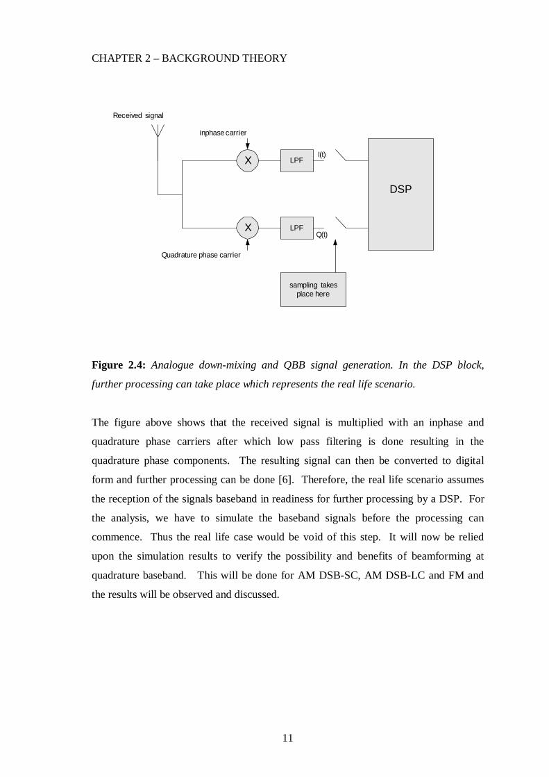
Figure 2.4: Analogue down-mixing and QBB signal generation. In the DSP block,

further processing can take place which represents the real life scenario.

The figure above shows that the received signal is multiplied with an inphase and

quadrature phase carriers after which low pass filtering is done resulting in the

quadrature phase components. The resulting signal can then be converted to digital

form and further processing can be done [6]. Therefore, the real life scenario assumes

the reception of the signals baseband in readiness for further processing by a DSP. For

the analysis, we have to simulate the baseband signals before the processing can

commence. Thus the real life case would be void of this step. It will now be relied

upon the simulation results to verify the possibility and benefits of beamforming at

quadrature baseband. This will be done for AM DSB-SC, AM DSB-LC and FM and

the results will be observed and discussed.

12


2.4 Multipath

Multipath is a form of interference and therefore it is undesired in radio propagation.

Some of the effects of multipath distortion include data corruption, increased signal

amplitude (constructive interference), reduced signal amplitude (destructive

interference), unwanted frequency response, co-symbol interference, etc [21]. In order

to mitigate the effects of multipath, a signal processing technique called ‘multipath

compensation’ is used. This implies that a receiver should be equipped with a

compensator that will eliminate the multipath effects and allow for the processing of the

desired direct-path signal only.

Multipath propagation plays a vital role in determining the nature of communication

channels. This implies determination of the impulse, or frequency response of radio

channels [20]. However, this study does not consider other channel factors in detail but

focuses on the compensation aspect of multipath. We will also ignore angular spread

and constriction effects since the main purpose of the study is to investigate the

possibility and benefits of compensating for multipath at QBB. It should also be noted

that we are using narrow band signals and noiseless channels are assumed. It is

required by this study to find out the possibility of compensating at baseband

frequencies as compared to the traditional RF methods and analyzing the benefits of

compensating at QBB.

2.4.1 Spectral changes due to time-shift in a signal

Time delay in a signal causes a linear phase shift in its spectrum. It does not change the

amplitude spectrum [3]. Suppose f(t) is being synthesized by its fourier components,

which are sinusoids of certain amplitudes and phases. It is seen that the delayed signal

f(t-to) can be synthesized by the same sinusoidal components, each delayed by to

seconds [27]. The amplitudes of the components remain unchanged. Therefore, the

amplitude spectrum of f(t-to) is identical to that of f(t). The time delay to in each

sinusoid does however change the phase of each component. It is therefore, seen that a

time delay to in a sinusoid frequency ω manifests as a phase delay of ωto. This is a

linear function of ω, which entails that higher-frequency components must undergo

proportionately higher phase shifts to achieve the same time delay. Let us now consider

13


the unit impulse response for the multipath channel. The response is expected to have

the direct path and delayed echo components. The mathematical expressions and

graphical plot for a delayed unit impulse are shown below.

( ) ( )

(1 )

( ) * ( ) * ( ( ) ( )) ( ) ( )

j

j

f t F e

H ke

f t H f t t k t f t kf t

ωτ

ωτ

τ ω

δ δ τ τ

−

−

− ↔= +

∴ = + − = + − (2.1)

The plot below illustrates the results above expressions.

0t

f(t)

1k

τ

Figure 2.5: Channel impulse response.

From the expressions above and assuming that the unit impulse is transmitted through a

multipath channel, it is seen that the convolution [27] between the unit impulse and the

channel H results in the direct path signal and an echo which is a delayed and scaled

down version of the direct path signal. In this case, the delayed signal is scaled down

by a factor ` k’.

2.4.2 RF and QBB Multipath compensation

In this part of the study as was explained for the beamforming case, the compensation

process is done at RF and then shifts to quadrature baseband in view of compensating

for multipath at QBB and utilising the benefits that come along with it. For the

multipath analysis, noiseless transmissions and narrow band signals were assumed.

14


2.5 Doppler shift

Doppler shift is another form of interference encountered in wireless communications.

Its effects are immense and the final result is that the received signal is distorted and

hence the need to compensate for the Doppler shift arising from motion between the

transmitting and receiving ends [25]. Doppler shift compensation restores the

frequency spectrum of the received signal by undoing the effects caused by the Doppler

shift. The simulations for this case will similarly be run at RF and QBB.

Frequency shifting

The frequency shift property of the Fourier transform forms the basis for our modeling

of a Doppler signal and its spectrum in MatLab. The duality between the time and

frequency domains does enable the frequency translation of a time domain signal by a

given value by multiplying the time domain signal with an exponent whose frequency is

equal to the required frequency shift [3]. The above statement is illustrated below:

( ) ( )f t F ω⇔ (2.2)

Multiplying a time function with the djw te yields the required frequency shift ‘dω ’.

( ) ( )

( ) ( )

d

d

j td

j td

f t e F

or

f t e F

ω

ω

ω ω

ω ω−

⇔ −

⇔ +

(2.3)

The expressions above thus entail the possibility of simulating the Doppler shift signal

by use of the frequency shifting property.

2.6 Multiple compensation

The study also looks at a scenario where multiple signals are received and summed up

together. The signals comprise the direct path signal, multipath signal, Doppler shift

signal and a signal that has been subjected to both multipath and Doppler shift effects. It

is required to compensate for the multipath and Doppler shift effects simultaneously.

15


This need not be confused with a MIMO system which has multiple inputs and multiple

outputs [36]. For the beamforming case, the presence of multiple antennas at the

transmitting and receiving ends creates a MIMO channel which offers significant

diversity [34]. The simulation results in Chapter 6 will show whether it is possible to

carry out multiple compensation.

2.7 Matched filtering :- Chirp signal

The study also carries out matched filter detection at RF and investigates the possibility

of doing so at QBB. A chirp signal will be used in the simulations. A chirp is a signal

whose frequency either increases or decreases with time [30]. A linear chirp is one

whose frequency varies linearly with time as shown in the expression on the next page.

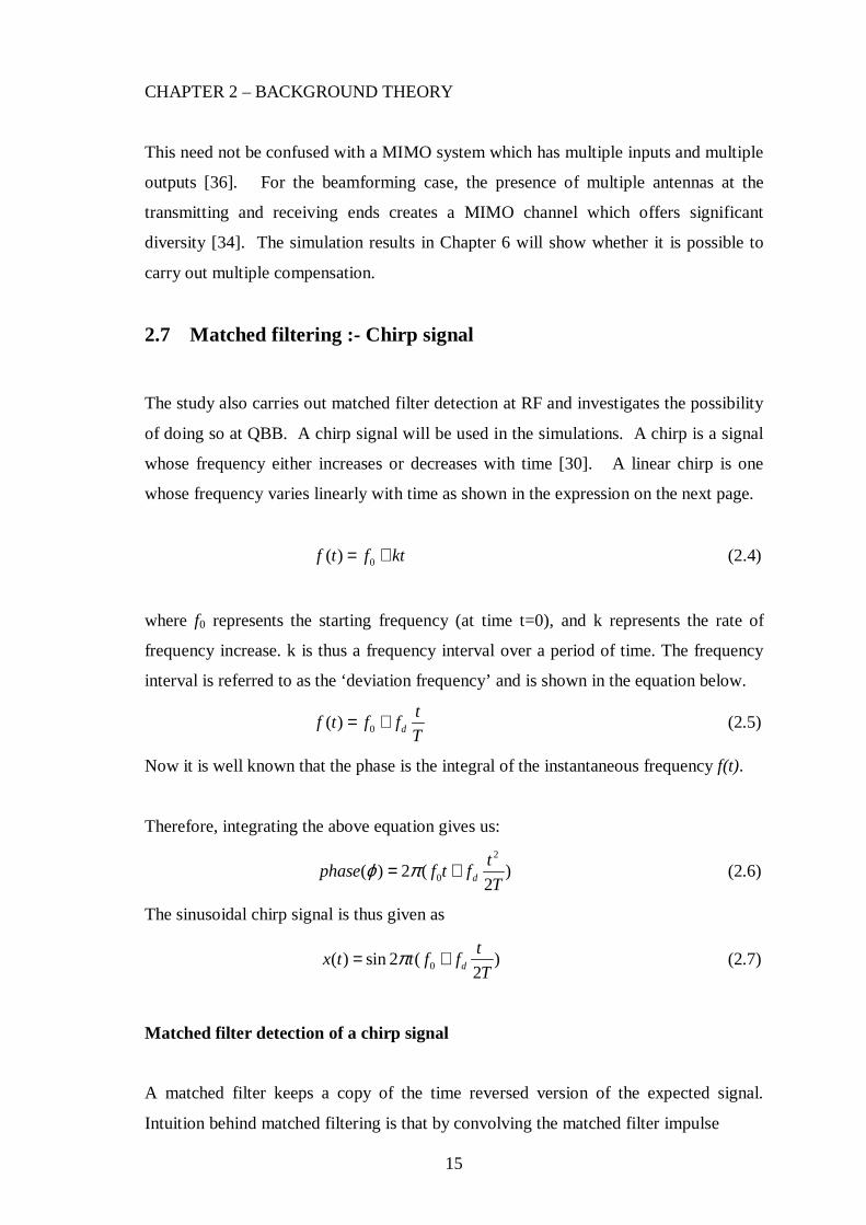
0( )f t f kt= + (2.4)

where f0 represents the starting frequency (at time t=0), and k represents the rate of

frequency increase. k is thus a frequency interval over a period of time. The frequency

interval is referred to as the ‘deviation frequency’ and is shown in the equation below.

0( ) d

tf t f f

T= + (2.5)

Now it is well known that the phase is the integral of the instantaneous frequency f(t).

Therefore, integrating the above equation gives us:

2

0( ) 2 ( )2d

tphase f t f

Tϕ π= + (2.6)

The sinusoidal chirp signal is thus given as

0( ) sin 2 ( )2d

tx t t f f

Tπ= + (2.7)

Matched filter detection of a chirp signal

A matched filter keeps a copy of the time reversed version of the expected signal.

Intuition behind matched filtering is that by convolving the matched filter impulse

16


response with the received signal (chirp), you are basically sliding across your time

reversed h(t) across your received signal doing a point wise multiplication and then

integrating over the area of that product [31]. Thus, the peak in the real part of the

output is only going to occur when the chirp in h(t) is exactly lined up with a chirp in

the received signal. In other words, the spike output corresponds to the point where the

greatest area underneath the curve is produced from the point-wise multiplication. The

location of the spike itself corresponds to the location of where the right most edge of a

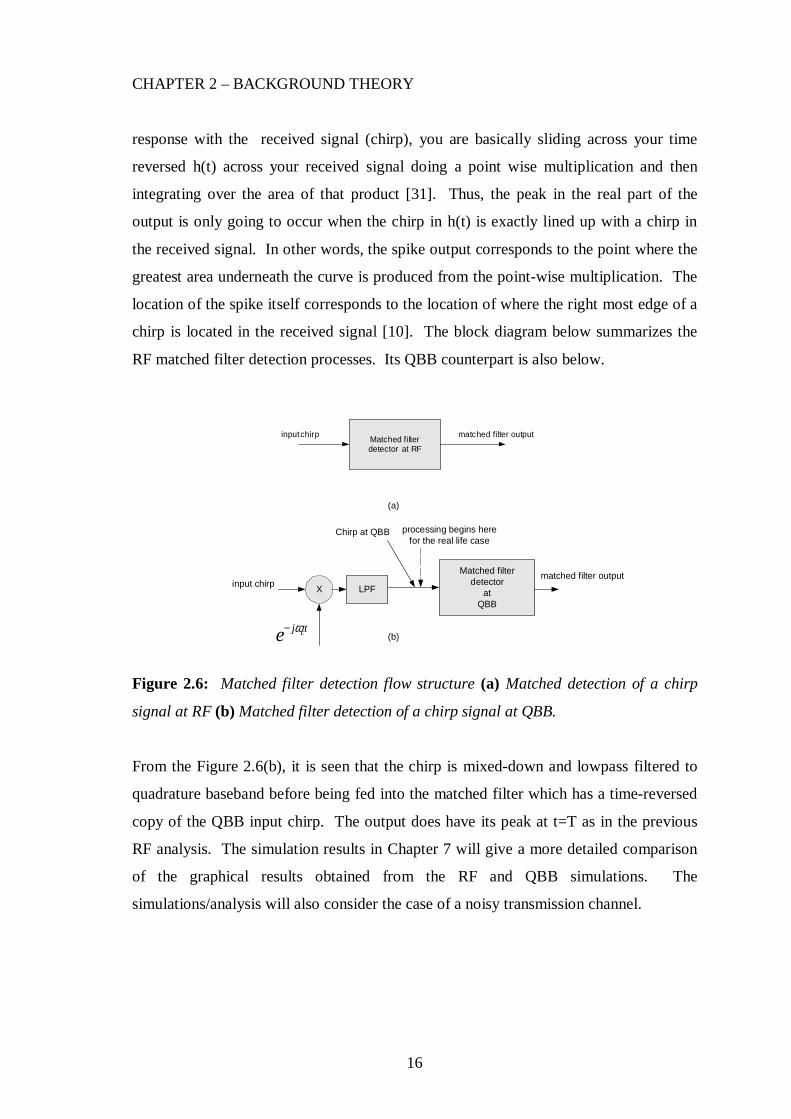
chirp is located in the received signal [10]. The block diagram below summarizes the

RF matched filter detection processes. Its QBB counterpart is also below.

Matched filterdetector

atQBB

input chirpmatched filter output

X

cj te ω−

LPF

Chirp at QBB

(b)

Matched filterdetector at RF

input chirp matched filter output

(a)

processing begins herefor the real life case

Figure 2.6: Matched filter detection flow structure (a) Matched detection of a chirp

signal at RF (b) Matched filter detection of a chirp signal at QBB.

From the Figure 2.6(b), it is seen that the chirp is mixed-down and lowpass filtered to

quadrature baseband before being fed into the matched filter which has a time-reversed

copy of the QBB input chirp. The output does have its peak at t=T as in the previous

RF analysis. The simulation results in Chapter 7 will give a more detailed comparison

of the graphical results obtained from the RF and QBB simulations. The

simulations/analysis will also consider the case of a noisy transmission channel.

17


2.8 AM DSB-SC, AM DSB-LC, FM and QAM

A brief summary of the 4 modulation schemes used in the simulations is given in the

following sub-sections. The focus is on carrying out the processing at QBB and hence

the demodulation at QBB for the selected modulation schemes is outlined.

2.8.1 AM DSB-SC

An Amplitude Modulated Double Sideband signal with Suppressed Carrier can be

represented by the equation shown below.

( ) ( )cos cm t f t tω= (2.8)

where f(t) is the message signal [3,4,12]. The modulated signal is then transmitted and

at the receiving end, the signal has to be demodulated.

QBB demodulation:- DSB-SC

Consider the figure shown below:

X Lowpass filter

(Local oscillator)

r(t)DSB-SC

Input Signal abs[qbb output]

Downmixing

cj te ω−

Figure 2.7: QBB demodulation block diagram.

The figure above shows that the demodulation of a DSB-SC quadrature baseband signal

is done by simply taking real part of the QBB signal and this gives the demodulated

signal. The QBB signal output is complex with the imaginary part being neglected and

hence taking the real part of this complex signal does give us the demodulated signal.

18


2.8.2 AM DSB-LC

The second modulation method that will be used in the simulations is AM DSB-LC.

The demodulation of a DSB-LC signal is done either coherently or non-coherently. The

non-coherent method being used here is envelope detection. A DSB-LC modulated

signal is given by the following expression [3, 12]:

m(t)=(Ac + mf(t))cos(ωct) (2.9)

where m= modulation index,

Ac= carrier amplitude,

Normalizing the carrier amplitude results in the following expression:

m(t)=(1 + mf(t))cos(ωct) (2.10)

AM DSB-LC QBB demodulation

For the QBB demodulation, the coherent and non coherent methods are used with the

coherent QBB demodulation method being similar to the DSB-SC method. For the

analysis, only the coherent QBB method was simulated.

2.8.3 FM

Unlike AM, FM is a non-linear type of modulation [8]. In our analysis, we will look at

a single-tone modulated FM signal. Assuming the modulating signal is a unit amplitude

sinusoid of the form m(t)=cos(ωmt), the FM modulated signal can be expressed as

( ) cos( .sin( ))c my t A t m tω ω= + (2.11)

where m represents the modulation index and is the ratio of the maximum frequency

deviation to the particular modulating frequency, fc is the carrier frequency (Hz), and Фc

is the initial phase (rads). θ(t) is the modulation phase, which changes with the

amplitude of the input m(t). The expression for θ(t) is given as

19


0

( ) ( )t

ot K m t dtθ = ∫ (2.12)

where Ko is the sensitivity factor, which represents the gain of the integrator output [8].

FM demodulation at QBB

On the other hand, FM QBB demodulation is done by unwrapping of the phase angle

using a MatLab command ‘unwrap’ followed by differentiating so as to give the

demodulated signal. The equation below illustrates this.

theta=unwrap(atan2(imag[s4],Real[s4])) (2.13)

where s4 is the QBB FM signal. The unwrapped angle is the differentiated as shown in

the equation on the next page.

s5=diff(theta) (2.14)

2.8.4 QAM (analogue)

The beamforming analysis modulation schemes that will be used are AM DSB-SC and

AM DSB-LC and FM. However, under multipath and Doppler shift we consider QAM

and FM. Before getting into the study of multipath compensation for QAM, it is

necessary to have a brief background about this modulation method. QAM modulates

an in-phase signal mI(t) and a quadrature signal mQ(t) using the expression shown

below:

( ) ( ). os ( )sin( )I c Q cy t m t c t m t tω ω= + (2.15)

Alternatively, a QAM signal may also be represented on the next page.

ˆ( ) ( ) cos( ) ( )sin( )c cy t m t t m t tω ω= + (2.16)

20


where m(t) represents a message signal and ˆ ( )m t is the Hilbert transform of m(t). It

should be noted that the expression above is for single side band QAM [22].

QAM demodulation at QBB

The QBB demodulation process is summarised by the block diagram below.

X LPF

Real(yqbb)

Imag(yqbb)

QAM input

down-mixed signal

QBB output

yqbb

Inphaseoutput

Quadrature phaseoutput

cj te ω−

Figure 2.8: QAM demodulation at QBB. After the mixing down process and lowpass

filtering, the real and imaginary parts of the resulting signal are taken resulting in the

inphase and quadrature phase outputs corresponding to the original inputs.

2.9 Channel / Compensator reciprocity

The study will carry out compensation for multipath, Doppler shift and also considers

multiple compensation. The aim of compensation is basically to retrieve the original

signal from the distorted received signal. A layman would say “the solution to a

problem lies in knowing the cause of the effect”. An engineer would paraphrase this

statement for the compensation case at hand and say “finding the compensator lies in

knowing characteristics of the channel”. By this is meant that in order to compensate

for an effect, the transfer function (channel) that caused the effect must be known. This

leads us to the reciprocity relationship between the channel and compensator illustrated

in the figure which follows. Thus, the compensator is seen as the inverse of the channel

transfer function. The simulations will verify this relationship. Will this relationship

hold for the multiple signal input case too? Chapter 6 adequately analyses and answers

this question. The block diagram on the next page illustrates this.

21


H(recieved signal

generating transferfunction)

Hc=1/H(Compensator)

Direct path signalReceived

signalCompensated output

signal

Figure 2.9: Channel/Compensator reciprocity structure.

2.10 Benefits of working at Quadrature baseband:- processor load

The focus of the study as mentioned earlier aims to verify possibility and the benefits of

working at QBB as compared to working at RF for selected demodulation algorithms

and compensation methods. The study will accomplish this by comparing two

parameters of the simulations run in MatLab. The main benefit of working at QBB

compared to RF is that the operating and sampling frequency is reduced. The other

benefit is derived from the sub-sampling carried out for the QBB case and for the

simulations, it will be assumed that the sub-sampling factor chosen would cause

limitations for the RF brought about by aliasing. Therefore, relative methods were

employed in order to quantify the sample processing. Chapter 3 illustrates how this was

done in the study. The processing time was also estimated using in-built Matlab

commands which measure the elapsed time between relevant parts of the simulation

code. This does not represent the true processing time that would take place in a DSP.

It is just a relative way of consolidating the processing load results as it expected that a

reduction in the processing load should result in a reduction in the processing time.

2.11 Conclusion

The chapter introduced the quadrature baseband theory and gave a brief overview of the

algorythms under investigation in this study. The modulation schemes used in the

analysis were also outlined. Flow diagrams were given so as to have an overview of the

general flow of the analysis that was carried out using MatLab simulations. The

procedure for finding out the benefits of working at QBB as compared working at RF

were also explained and as mentioned, Chapter 3 will give a more detailed outline of

this procedure. With this background theory discussed in this chapter, the analysis and

discussion of the simulations results takes place in the chapters that follow.

22

Chapter 3 Beamforming- simulation results

The MatLab simulation results for beamforming at RF and QBB for the selected

modulation schemes are given and discussed in this chapter. The theoretical analysis

for each method is given and the RF and QBB results compared, discussed and a

summary of the results is given. The study does indeed show the possibility of

beamforming at QBB. The chapter concludes by comparing the RF and QBB

simulations in terms of simulation runtime and number of processing calculations for

the signal samples processed by the simulations. Does QBB come out advantageous in

this case? The latter part of the chapter should answer this question.

3.1 RF beamforming

In this analysis, four input signals are summed up together and the summed up signal is

demodulated and then a beam pattern is produced. Earlier in Chapter 2, the RF and

QBB beamforming processes where outlined.

Theoretical Analysis

A theoretical summary of the RF beamforming process is given below. The reference

signal is the non-delayed sinusoidal input s0. The reference signal in this case is the

AMDSB-SC/AMDSB-LC or FM input depending on which modulation scheme is

being analyzed. Therefore, taking s0 as the reference signal, we generate 3 other signals

with a fixed delay separation in between each signal.

1 0

2 0

3 0

( )

( 2 )

( 3 )

s s t t

s s t t

s s t t

= − ∆= − ∆= − ∆

(3.1)

The 4 signals were summed up to give the signal s4. This represents a simple

beamforming stage of the analysis.

23

CHAPTER 3 – BEAMFORMING: SIMULATION RESULTS

s4=s0+s1+s2+s3 (3.2)

The beamformed signal is then demodulated using the demodulation method for each

modulation scheme as outlined in Chapter 2 resulting in the demodulated signal which

is denoted as s5. The size of the demodulated signal is then determined so as to get the

beam pattern. The figure below summarises the theoretical analysis beam forming at

RF.

4 e lem e n t A n ten na a rra y

B ea m fo rm in g a t R F

D em od u la t io n

Incom ing de la ye ds igna ls

D e m odu la te do u tp u t + B ea m

p a tte rn

0s 1s2s 3s

4s

5s

sa m p lin g ta ke sp la ce h e re

Figure 3.1: RF Beamforming theoretical analysis block diagram.

The block diagram above basically illustrates the processing of the signal from the input

up to the final stage of forming the beam pattern. The delayed signals are thus arriving

at the antenna array from a range of angles and the result of the signal size is stored up

to the last value of theta. For the simulations carried out, the incoming signals were

sampled before the beamforming stage. The beam pattern is then produced by taking

the maximum signal size and making a polar plot against theta.

24


3.2 Quadrature Baseband (QBB) Beamforming

The idea of quadrature baseband beamforming involves carrying out beamforming at

quadrature baseband frequencies. The procedure under QBB involves mixing down the

four incoming signals to baseband and then lowpass filtering to get their quadrature

baseband equivalents. The beamforming takes place at quadrature baseband after which

demodulating the summed signal follows from which the maximum value of the output

signal is taken so as to make a polar plot. For the simulations carried out, the four

incoming signals are mixed down to baseband using a local oscillator having an

exponential complex and then lowpass filtered to convert our down-mixed signals to

quadrature baseband signals. Sub-sampling is done followed by QBB demodulation

from which the beam pattern was derived.


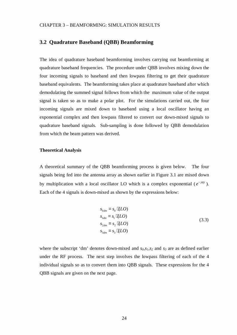
A theoretical summary of the QBB beamforming process is given below. The four

signals being fed into the antenna array as shown earlier in Figure 3.1 are mixed down

by multiplication with a local oscillator LO which is a complex exponential ( cj te ω− ).

Each of the 4 signals is down-mixed as shown by the expressions below:

0 0

1 1

2 2

3 3

( )

( )

( )

( )

dm

dm

dm

dm

s s LO

s s LO

s s LO

s s LO

= ⋅= ⋅= ⋅= ⋅

(3.3)

where the subscript ‘dm’ denotes down-mixed and s0,s1,s2 and s3 are as defined earlier

under the RF process. The next step involves the lowpass filtering of each of the 4

individual signals so as to convert them into QBB signals. These expressions for the 4

QBB signals are given on the next page.

25


0 0 1 1

2 2 3 3

[ ] , [ ]

[ ] , [ ]

qbb dm LPF qbb dm LPF

qbb dm LPF qbb dm LPF

s s s s

s s s s

= =

= = (3.4)

At this stage we have four QBB signals and the downsampling process can take place at

this stage. This is done by taking every nth sample of the signal where n represents the

downsampling factor. The downsampled version of s0qbb is obtained as follows in

MatLab:

0 0 1 1

2 2 3 3

(1: : ), (1: : )

(1: : ), (1: : )

qbbds qbb qbbds qbb

qbbds qbb qbbds qbb

s s n end s s n end

s s n end s s n end

= =

= = (3.5)

Beamforming can now take place at this stage.

s4=s0qbbds+s1qbbds+s2qbbds+s3qbbds (3.6)

To get our demodulated output signal, the absolute value of s4 is taken and this gives us

our quadrature baseband demodulated out put signal.

5 4[ ]s abs s= (3.7)

The maximum of s5 is then taken and a polar plot is done to give us the required beam

pattern. The block diagram on the next page summarizes the theoretical analysis for

beamforming at QBB. As was mentioned earlier in Chapter 2, the QBB signals are

generated by the simulation before the beamforming can take place. As explained

earlier in Chapter 2, representing the real-life analogue processing is basically the same

as that for the simulated representation but with the down-mixing and lowpass filtering

stages skipped which precede the sampling process. Figure 3.2 on the next page

summarises the QBB beamforming process.

26


4 element Antenna array

Incoming Inputsignals

X X X X

Local oscillator

LPF LPF LPF LPF

Beamforming at QBB

QBB Demodulation

DemodulatedOutput+ Beam

pattern

( )cj te ω−

Downsampling

4s

5s

0dms 1dms2dms 3dms

3qbbs2qbbs1qbbs0qbbs

0s1s 2s 3s

sampling takes placehere

Figure 3.2: Quadrature baseband beamforming theoretical analysis block diagram. It

is seen from the diagram that the signal outputs at each stage have been shown. The

figure above represents the beamforming process for the simulated QBB signals. The

real life scenario representation would skip the generation stage and proceed with the

processing of the analogue down-mixed QBB signals. It will be seen when analysing

the benefits in terms of processor load of how the simulated and real life scenario QBB

method compare with the simulated RF results.

27


3.3 Simulation results – AM DSB-SC

This chapter analyses and discusses the actual simulation results of the MatLab analysis

of RF and QBB beamforming. The beam pattern shapes are also controlled by factors

like the antenna spacing and array factor [11, 19]. For the analysis, parameters like the

antenna weight were normalised for simplicity’s sake.

Simulation results: - RF Beamforming

The graphical results below result from RF beamforming simulations.

0 50 100 150 200 250 300 350 400 450 500-8

-6

-4

-2

0

2

4

6

8Summed signal

samples

am

plit

ud

e

0 50 100 150 200 250 300 350 400 450 500-8

-6

-4

-2

0

2

4

6

8summed signal * carrier(Local oscillator)

samples

am

plit

ud

e

(b)

0 50 100 150 200 250 300 350 400 450 500-8

-6

-4

-2

0

2

4

6

8Demodulated signal

samples

am

plit

ud

e

(c)

10

20

30

40

50

30

210

60

240

90

270

120

300

150

330

180 0

beam pattern

(d)

(a)

Figure 3.3: Simulation results.(a) Summed signal (b) Summed signal multiplied with

carrier (c) Demodulated output (d) Beam pattern.

28


The simulation results obtained for RF beamforming for the signals being received by

the antenna array are now analyzed. In Figure 3.3(a) it seen that there are three cycles

for the 512 samples of the summed up signal. The local oscillator translates the

frequency of the summed signal to 2fc on the frequency spectrum where fc represents the

carrier frequency. This is done in order to facilitate for the demodulation of the

summed signal using the AMDSB-SC demodulation method outlined earlier in Chapter

2. The resulting demodulated output is shown in Figure 3.3(c). Plotting the maximum

of the demodulated output against theta yields the beam pattern shown in Figure 3.3(d)

and consists of the main beam and side lobes. It is a well known fact that side lobes are

undesirable in any beam pattern because they reduce the energy in the main beam. The

resulting beam pattern has a maximum value of approximately 40 and has 6 sidelobes.

The study is yet to come to its fulfilment because, we now have to carry out

beamforming at quadrature baseband and compare the two results.

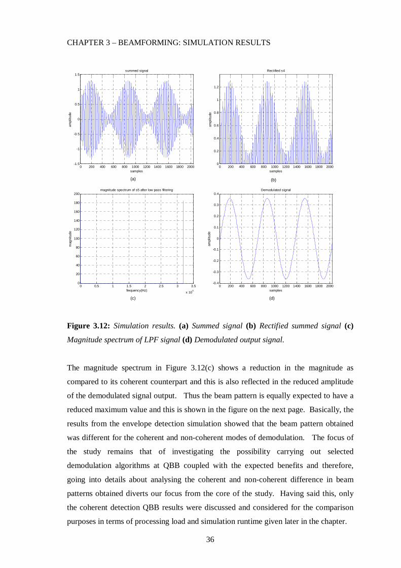
3.3 Simulation results - QBB Beamforming

The analysis moves down to quadrature baseband where beamforming will now take

place. The signals now sit at QBB facilitating for beamforming at QBB. Sub-sampling

which takes place before the beamforming and in this particular simulation, the sub-

sampling factor was 4. Therefore, as can be seen from the demodulated output, there is

a 4-fold reduction in the number of samples down to 128 samples as compared to the

initial 512 samples that the input signals had. It is seen that this does not affect the

demodulated output as well as the beam the resulting pattern. In actual fact, this

presents an advantage of the beamforming at QBB in that the same results as at RF can

be produced but with fewer samples. The beamformed signal is then demodulated

using QBB demodulation by taking the real part of the QBB signal resulting in the

demodulated output shown in Figure 3.4(a) on the next page and the corresponding

beam pattern shown in Figure 3.4(b).

29


0 20 40 60 80 100 120-8

-6

-4

-2

0

2

4

6

8demodulated signal

samples

ampl

itude

10

20

30

40

30

210

60

240

90

270

120

300

150

330

180 0

beam pattern

(a) (b)

Figure 3.4: Simulation plots (a) Demodulated signal (b) Beam Pattern.

Are there any changes in the results obtained at QBB as compared to its RF

counterpart? The beam pattern produced should answer the question. Compared to the

RF demodulated signal output, it is seen that the two signals are the ‘same’ having the

same amplitude and frequency characteristics and therefore, we expect to have similar

beam patterns. However, the visual similarity can not be substantiated unless it

accompanied by numerical backing. Therefore, the next section will verify the

similarity between the RF and QBB beam patterns by plotting the numerical difference

between them.

3.4 Beam pattern comparisons

The beam patterns are now shown together in Figure 3.5 on the next page for easy

analysis and comparison of the patterns. In order to numerically prove the similarity

of the two beam patterns, a MatLab program was created to carry out the numerical

comparison. The program incorporates the two beamforming codes (RF and QBB) and

then gets the difference between the normalized beam patterns is shown in figure 3.6(b)

on the next page.

30


10

20

30

40

50

30

210

60

240

90

270

120

300

150

330

180 0

beam pattern

(a) (b)

10

20

30

40

30

210

60

240

90

270

120

300

150

330

180 0

beam pattern

Figure 3.5: Beam pattern comparisons (a) RF beam pattern (b) QBB beam pattern.

The error/difference plot is given below.

INPUTPARAMETERS

AM DSB-SC RFBeamforming

AM DSB-SC QBBBeamforming

Beam pattern Beam pattern

Comparison of beampatterns & Difference

plot

Difference plot

(a) (b)

0 50 100 150 200 250 300 350

0

0.5

1

1.5

2

2.5

3

3.5

4

4.5

x 10-3 difference plot for RF and QBB beam patterns

theta (degrees)

ampl

itude

Difference/Error plot

Figure 3.6: (a) Difference plot flow diagram (b) Difference plot.

It is clearly seen that the difference between the two plots is minimal and therefore, it

suffices to say that the two beam patterns are similar and that it has been verified that

beamforming at QBB gives a similar beam pattern to its RF counterpart. Therefore,

suffices to say that beamforming at quadrature baseband is possible and this comes with

31


its main advantage of working at lower sampling frequencies unlike for the high RF

frequencies.

3.6 MatLab Analysis Simulation Results: –AM DSB-LC

3.6.1 Beamforming: AM DSB-LC

This part of the study analyses RF beamforming for another AM modulation technique

AM DSB-LC. The two methods being considered are the Coherent method and the

Envelope detector (non-coherent). The MatLab analysis results are also shown and

discussed in this chapter. The modulation method being analyzed is AM DSB-LC.

There is a difference in the way an AM DSB-SC and AM DSB-LC signal is represented

which is evidenced by the expressions given in Chapter 2. The demodulation of a DSB-

LC signal is done either coherently or non-coherently. The non-coherent method being

used here is envelope detection.

3.6.2 Coherent and Non-Coherent (Envelope) detection methods

As mentioned already in Chapter 2, two methods will be used to carry out our RF

analysis of the beamforming process for the AMDSB-LC signals so as to see any

changes that take place in the beam pattern shape when the detection process is done

coherently and non-coherently. We have the coherent and the non-coherent method of

which the latter is also referred to as the envelope detector. The flow diagram on the

next page is a structural summary of the whole RF analysis that was used in the MatLab

simulations.

32


Begin

Define input parameters

Beamforming at RFAM DSB-LC

Envelope Detection Coherent Detection

Demodulated OutputSignal

Demodulated Output

Beam pattern Beam Pattern

s4 s4

s5 s5

Figure 3.7: AM DSB-LC beamforming at RF analysis structure flow diagram. The same

analysis applies for the QBB case though for the QBB case, only the coherent case was

looked at to avoid repetition in the analysis.

3.6.2.1 Coherent detection

The detection process under this method is done by multiplying the summed signal with

a local oscillator whose frequency is synchronized to the carrier frequency. i.e

s5=s4(LO). The demodulated output is give below as

s5=[s5]LPF. (3.8)

The amplitude of s5 is the taken and a polar plot of the amplitude against theta is done to

give the beam pattern.

33


3.6.2.2 Envelope detection

Under this detection method, the summed signal is rectified using a half-wave rectifier

(HWR) and then the rectifier output is lowpass filtered to give the demodulated output

signal [33]. The envelope detector circuit is given earlier in Chapter 2. The expression

below illustrates the process.

s4r= [s4]HWR (3.9)

The demodulated output is the lowpass filtered version of s4r .

s5=[s4r]LPF (3.10)

This gives us the demodulated output from which our beam pattern will be formed by

taking the maximum value of the output and making a polar plot.

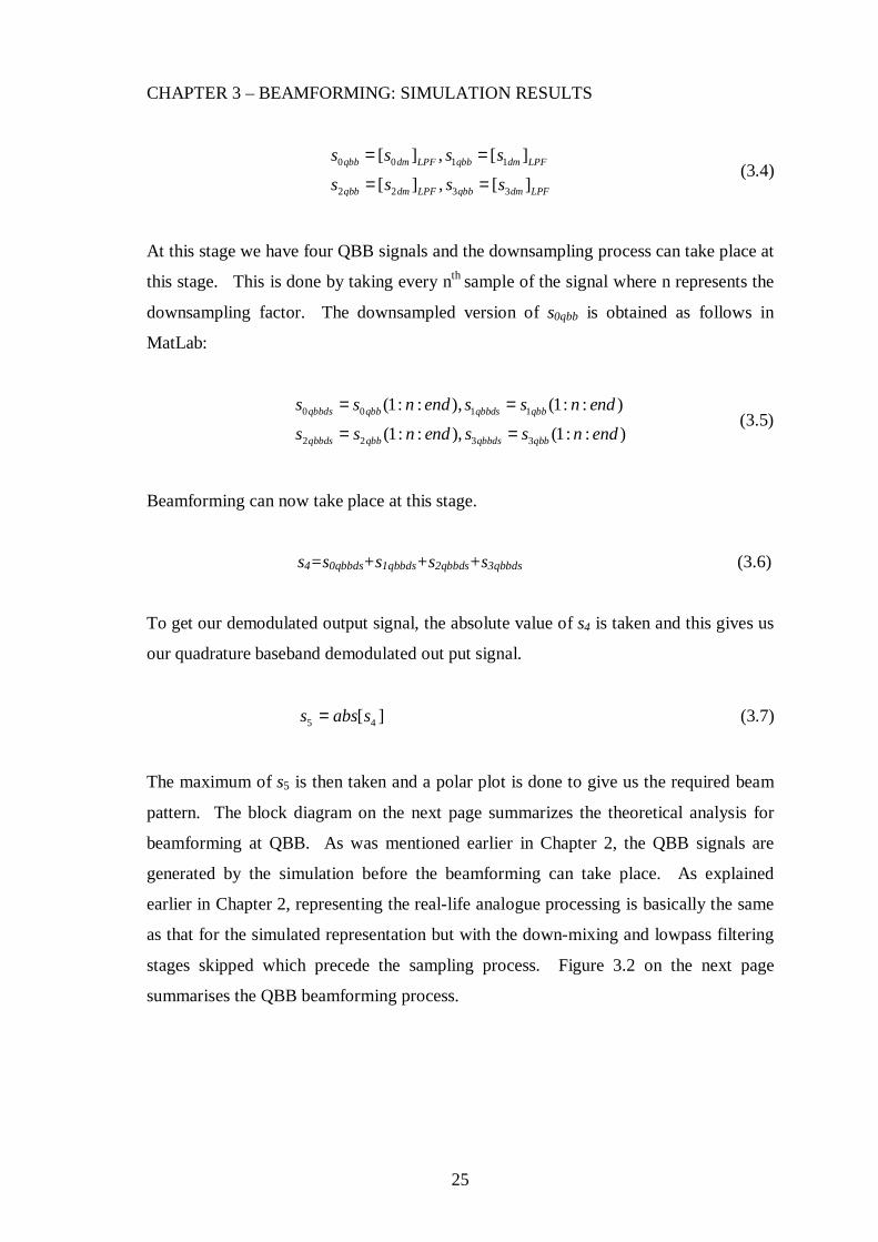
3.6.3 Simulation results:- AMDSB-LC Beamforming at RF

The simulation results for beamforming at RF for the coherent and non-coherent

method are given in the following sections. For this simulation the number of samples

was increased to 2048 and the sampling frequency used was 32000Hz.

3.6.3.1 Coherent detection

This method as already explained earlier does employ a local oscillator whose

frequency is equal to the carrier frequency. The block diagram shown below is an

illustration of the MatLab code which is used in this analysis.

Set inputparameters

Define loop,delaysand signal inputs

beamforming +demodulation ofsummed signal

Max ofdemodulated

signal andformation of beam

pattern

beam pattern

Figure 3.8: MatLab code structure:-Coherent detection.

34


Figures 3.9(a), (b), (c) and (d) below illustrate the graphical results of our MatLab

analysis. The beamformed / summed signal in Figure 3.9(a) is multiplied with the local

oscillator frequency and this translates the low frequency summed up signal to + 2ωc on

the frequency spectrum. The resulting signal is shown in Figure 3.9(b). The higher

(double) frequency components are then effectively filtered out by a low pass filter

resulting in the spectrum shown in Figure 3.9(c). The resulting demodulated signal is

shown in Figure 3.9(d).

0 200 400 600 800 1000 1200 1400 1600 1800 2000-1.5

-1

-0.5

0

0.5

1

1.5summed signal

samples

ampl

itude

(a)

0 200 400 600 800 1000 1200 1400 1600 1800 2000-0.2

0

0.2

0.4

0.6

0.8

1

1.2

Summed signal*LO

samples

ampl

itude

0 0.5 1 1.5 2 2.5 3 3.5

x 104

0

50

100

150

200

250

300magnitude spectrum of s5 after low pass filtering

frequency(Hz)

mag

nitu

de

0 200 400 600 800 1000 1200 1400 1600 1800 2000-0.8

-0.6

-0.4

-0.2

0

0.2

0.4

0.6

0.8Demodulated signal

samples

ampl

itude

(d)

(b)

(c)

Figure 3.9: Simulation plots.(a) Summed signal (b) Summed signal*Local oscillator (c)

Magnitude Spectrum after LPF. (d) Demodulated output signal.

A polar plot of the maximum value of the demodulated output gives the required beam

pattern entailing the successful beamforming process using the coherent method. The

resulting beam pattern is given in the figure on the next page.

35


1

2

3

4

30

210

60

240

90

270

120

300

150

330

180 0

beam pattern

Figure 3.10: Beam pattern.

3.6.3.2 Envelope Detection

The beamforming was now carried out for the non-coherent method which is also

referred to as the envelope detector. It will be interesting to see the changes that take

place in the resulting beam pattern from this type of demodulation. The block diagram

shown below illustrates the MatLab code used for the analysis.

Set inputparameters

DefineLoop,delays and

signal inputs

Beamforming,1/2wave rectification

+demodulation

max ofdemodulatedoutput +beam

pattern

Beam pattern

Figure 3.11: Matlab code structure:-Envelope detector simulation.

The simulation results are given in the figures on the next page. The beamformed

signal remains the same as in the coherent case. The summed signal was passed

through a simulated half-wave rectifier where it was seen that the diode in the rectifier

clips out the negative cycles of the signal leaving the positive cycles from which our

envelope will be extracted.

36


0 200 400 600 800 1000 1200 1400 1600 1800 2000-1.5

-1

-0.5

0

0.5

1

1.5summed signal

samples

ampl

itude

0 200 400 600 800 1000 1200 1400 1600 1800 20000

0.2

0.4

0.6

0.8

1

1.2

Rectified s4

samples

ampl

itude

(b)

0 0.5 1 1.5 2 2.5 3 3.5

x 104

0

20

40

60

80

100

120

140

160

180

200magnitude spectrum of s5 after low pass filtering

frequency(Hz)

mag

nitu

de

0 200 400 600 800 1000 1200 1400 1600 1800 2000-0.4

-0.3

-0.2

-0.1

0

0.1

0.2

0.3

0.4Demodulated signal

samples

ampl

itude

(a)

(c) (d)

Figure 3.12: Simulation results. (a) Summed signal (b) Rectified summed signal (c)

Magnitude spectrum of LPF signal (d) Demodulated output signal.

The magnitude spectrum in Figure 3.12(c) shows a reduction in the magnitude as

compared to its coherent counterpart and this is also reflected in the reduced amplitude

of the demodulated signal output. Thus the beam pattern is equally expected to have a

reduced maximum value and this is shown in the figure on the next page. Basically, the

results from the envelope detection simulation showed that the beam pattern obtained

was different for the coherent and non-coherent modes of demodulation. The focus of

the study remains that of investigating the possibility carrying out selected

demodulation algorithms at QBB coupled with the expected benefits and therefore,

going into details about analysing the coherent and non-coherent difference in beam

patterns obtained diverts our focus from the core of the study. Having said this, only

the coherent detection QBB results were discussed and considered for the comparison

purposes in terms of processing load and simulation runtime given later in the chapter.

37


0.5

1

1.5

2

2.5

30

210

60

240

90

270

120

300

150

330

180 0

beam pattern

Figure 3.13: Beam pattern

3.6.4 Simulation results:- AMDSB-LC Beam forming at QBB

The simulation for the QBB analysis was done for the coherent and non-coherent

methods though only the coherent method was discussed below due to the fact that the

results obtained for the two methods are similar and as required by focus of the study,

we basically aim to show that processing carried out at RF can equally be carried out at

QBB with the processing load expected to be less at QBB which will be verified later in

the chapter. The block diagram below illustrates the MatLab code structure.

Define inputparameters

Define loop delaysand signal inputs

+ down-mixing

LPF to get QBBsignals+

Downsampling

Beamforming +QBB

demodulation +beam pattern

formation

Beampattern

Figure 3.14: MatLab code structure.

Figures 3.15(a), (b), (c) and (d) on the next page are the simulation results obtained for

the beamforming process at QBB. The input parameters used in the simulation were the

same as those used for the two RF methods and hence this will facilitate for the correct

comparison of the beam pattern outputs for the two procedures (RF and QBB). The

procedure for the beamforming remains the same as explained earlier for the AMDSB-

SC process and hence the earlier explanation given does suffice in explaining the

current situation. Figure 3.15(a) represents the complex QBB beamformed signal and

its magnitude spectrum in Figure 3.15(b). The magnitude spectrum is plotted in terms of

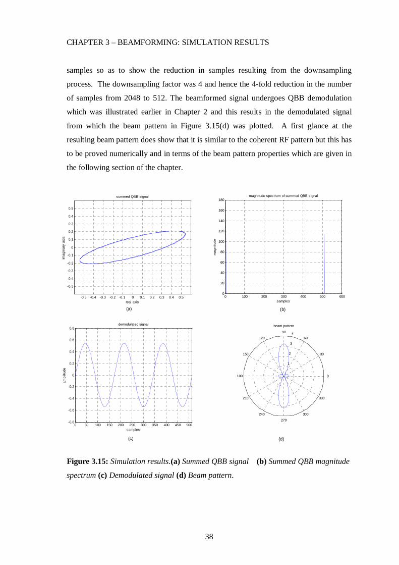
38


samples so as to show the reduction in samples resulting from the downsampling

process. The downsampling factor was 4 and hence the 4-fold reduction in the number

of samples from 2048 to 512. The beamformed signal undergoes QBB demodulation

which was illustrated earlier in Chapter 2 and this results in the demodulated signal

from which the beam pattern in Figure 3.15(d) was plotted. A first glance at the

resulting beam pattern does show that it is similar to the coherent RF pattern but this has

to be proved numerically and in terms of the beam pattern properties which are given in

the following section of the chapter.

0 50 100 150 200 250 300 350 400 450 500-0.8

-0.6

-0.4

-0.2

0

0.2

0.4

0.6

0.8demodulated signal

samples

ampl

itude

1

2

3

4

30

210

60

240

90

270

120

300

150

330

180 0

beam pattern

(d)

0 100 200 300 400 500 6000

20

40

60

80

100

120

140

160

180magnitude spectrum of summed QBB signal

samples

mag

nitu

de

(a) (b)

(c)

-0.5 -0.4 -0.3 -0.2 -0.1 0 0.1 0.2 0.3 0.4 0.5

-0.5

-0.4

-0.3

-0.2

-0.1

0

0.1

0.2

0.3

0.4

0.5

summed QBB signal

real axis

imag

inar

y ax

is

Figure 3.15: Simulation results.(a) Summed QBB signal (b) Summed QBB magnitude

spectrum (c) Demodulated signal (d) Beam pattern.

39


3.6.5 Beam pattern comparisons

As with the previous analysis, the beam patterns resulting from the analysis done are

compared so as numerically verify the similarity of the beam patterns. The figure below

shows the comparison structure and resulting error plot.

Coherent method RFbeamforming

Coherent method QBBbeamforming


Comparison of beam patterns(numerical difference)

Differnce/error plot

Input parameters

(a) (b)

0 50 100 150 200 250 300 350

-6

-5

-4

-3

-2

-1

0

1

2

x 10-4 difference/error plot

theta (degrees)

ampl

itude

Figure 3.16: (a) MatLab simulation structure for beam pattern comparison (b)

Difference/error plot: the error is very minimal and thus the beam patterns are similar.

3.7 MatLab Analysis Simulation Results:– Frequency Modulation

The results of the FM beamforming simulations are outlined in this section and a

numerical comparison is made between the resulting beam patterns and draws up a

conclusion over the possibility of beamforming at QBB

3.7.1 Simulation results:– Beamforming for FM at RF

The analysis results for RF beam forming for FM are given and discussed below. For

this analysis, the sampling frequency used was 3000Hz, the deviation was 100Hz, and

40


the number of samples used to represent a signal was 512. The Matlab code structure is

the same as that given earlier in the chapter. The figures that follow are the simulation

results obtained at RF. The summed signal in Figure 3.17(a) resulted in the magnitude

spectrum in Figure 3.17(b). From the spectrum it is seen that the signal sits at ‘fc’ and

has harmonics spreading out on the spectrum. The in-built ‘fmdemod’ Matlab function

effectively demodulates the beamformed signal and which is shown in Figure 3.17(c).

The resulting beam pattern is given in 3.17(d).

0 50 100 150 200 250 300 350 400 450 500-10

-5

0

5

10

15summed signal

samples

ampl

itude

0 500 1000 1500 2000 2500 30000

100

200

300

400

500

600

700

800

900

1000magnitude spectrum of summed signal

frequency(Hz)

mag

nitu

de

0 50 100 150 200 250 300 350 400 450 500-1.5

-1

-0.5

0

0.5

1

1.5output signal

samples

ampl

itude

(c)

0.2

0.4

0.6

0.8

1

30

210

60

240

90

270

120

300

150

330

180 0

beam pattern

(d)

(a)(b)

Figure 3.17: Simulation results (a) Summed signal (b) Magnitude spectrum of summed

signal (c) Demodulated output signal (d) Normalised beam pattern.

41


3.7.2 Simulation results:-Beamforming for FM at QBB

The graphical results below show quadrature baseband beam forming for FM signals.

The demodulation of FM signals at QBB was outlined earlier in Chapter 2. The

conditions and parameters used are the same as at for the RF simulation. The sampling

frequency being 3000Hz and the number of samples 512. The summed QBB signal and

its downsampled spectrum are shown in Figures 3.18 (a) and (b) respectively. The

downsampling factor was 2 and hence the 2-fold reduction in the number of samples.

The demodulated signal and the resulting beam pattern are shown in Figure 3.18(c) and

(d) respectively on the next page.

0 50 100 150 200 250-1.5

-1

-0.5

0

0.5

1

1.5summed-up demodulated signal

samples

ampl

itude

(c)

0.2

0.4

0.6

0.8

1

30

210

60

240

90

270

120

300

150

330

180 0

beam pattern

(d)

0 50 100 150 200 2500

200

400

600

800

1000

1200magnitude spectrum of QBB signal

samples

mag

nitu

de

(b)

-10 -8 -6 -4 -2 0 2 4 6 8 10-10

-8

-6

-4

-2

0

2

4

6

8

10summed complex baseband signal

real axis

imag

inar

y ax

is

(a)

Figure 3.18: Simulation results (a) Summed QBB signal (b) Magnitude spectrum of

summed QBB signal (c) Demodulated signal output (d) Normalised beam pattern.

42


The RF and QBB beam patterns look similar and it will be validated by the numerical

proof in the following section where a difference plot will show the actual numerical

difference between the two beam patterns.

3.7.3 Numerical Comparison of beam Patterns

The normalised beam patterns for the RF and QBB beamforming were compared

numerically using a MatLab program. The figure below shows the difference plot flow

between the two beam patterns produced and the error/difference plot against theta

(degrees).

INPUT PARAMETERS

FM RF Beamforming FM QBB Beamforming


Comparison of beampatterns & Difference

plot

Difference plot

(a)

0 50 100 150 200 250 300 350 4000

0.5

1

1.5

2

2.5

3

3.5

4

4.5

5x 10

-3 difference plot for RF and QBB beam patterns

theta (degrees)

ampl

itude

difference plot

b

Figure 3.19: (a) Difference plot Matlab structure flowchart. (b) Difference plot.

From the difference plot between the two beam patterns, it is seen that the two beam

patterns match perfectly/precisely and so, it suffices to say that the two beam patterns

are similar and that it has been verified that beamforming in QBB gives a similar beam

pattern to its RF counterpart. This justification also entails that beamforming can be

done at quadrature baseband which for reasons already mentioned; does have more

advantages than the traditional RF method. The Table 3.3 on the next page further

illustrates the beam pattern properties for the beam patterns plotted under the FM

simulations. It is seen that the two patterns match in terms of the pattern properties and

43


hence substantiating the purpose of this part the study which aims to beamform at QBB

and achieve the same results as at RF. The benefits in terms of processing load and

time of QBB versus RF beamforming will be seen in the next section of the chapter.

3.8 Benefits of beamforming at quadrature baseband

The benefits of beamforming at quadrature baseband can be expressed in terms of the

sampling frequency. The fast growing telecommunications industry does strive to

make efficient and effective use of the available resources of which bandwidth is very

significant. The benefits of processing at QBB were investigated and a conclusion was

drawn from the results obtained from the simulation runtimes and theoretical

calculations based on the simulation code.

3.8.1 Sampling frequency and bandwidth

According to nyquist’s criterion [4], the sampling frequency must be at least twice the

bandwidth.

2( )2s c

Bf f≥ + (3.11)

where B represents the signal bandwidth. Consider the figure shown below.

cff

sfs cf f−2c

Bf +

2c

Bf −

B

Power

0

Figure 3.20: RF/QBB sampling frequency comparison.

Referring to the figure above, the sampling frequency for the signal at RF is twice the

sum of the carrier frequency and signal bandwidth. And hence this entails that the

beamforming at RF is done at a higher frequency too. However, looking at the

44


QBB case, the required bandwidth is equal to the signal bandwidth itself and this is

because the carrier frequency is eliminated by the shifting down process. The

percentage saving in terms of sampling frequency is significant in ensuring more

efficient usage of available resources like bandwidth. The mathematical derivation of

the saving is given below. Let fsqbb denote the QBB sampling frequency and fsrf the RF

sampling frequency. The ratio of fsqbb to fsrf is found as follows:

0| 2( ) |

2

2( )2

csqbb c f

sqbb

Bf f

Bf B

=≥ +

≥ = (3.12)

Similarly

2( )

22

srf c

srf

Bf f

f fc B

≥ +

= + (3.13)

The required ratio is given below.

2 2

sqbb

srf c c

f B B

f f B f B∴ = =

+ + (3.14)

Assuming fc =1000Hz and B=40Hz, then the percentage saving by working at QBB in

terms of bandwidth is calculated below:

40 1

2040 51sqbb

srf

f

f∴ = = (3.15)

The percentage saving is thus equal to

(2040 40)

100 98%2040

− × ≈

Therefore, the above ratio shows a very significant saving being achieved by operating

at QBB in terms of the sampling frequency [2].

When fc=0.5B

This worst case scenario assumes that fc=0.5B. Therefore, considering Equation 3.14, B

is neglected and the ratio reduces to ½. This implies that the minimum saving in terms

of sampling frequency reduction that can be achieved is 50%.

45


When fc >>B

This scenario presents another extreme case. From Equation 3.14, it is seen that for this

particular case, the ratio fsqbb: fsrf approaches 1/2fc.

3.8.2 Sample processing and simulation time

This aspect of showing the savings achieved from working at QBB looks at the number

of calculations in the simulation code carried out RF and QBB in terms of ‘N’ which

represents the number of samples. Therefore, the MatLab code for the RF and QBB

simulations was redefined in terms of N. The filtering process involves taking the FFT

and then killing off the unwanted part of the spectrum by multiplication with the filter

response and then taking the IFFT to get back to the time domain. It is already known

that carrying out an FFT involves NLog2N multiplications when N is a power of 2 [7].

The same is assumed for the IFFT. As mentioned earlier the processing load was

measured using a relative method. The simulation runtime was measured using the

inbuilt Matlab [5] commands ‘tic’ and ‘toc’. Therefore, timers were introduced into the

simulations so as to measure the elapsed time for each simulation. It should be noted

that the time and numerical calculation measurements start from the received signal

models down to the demodulation as this is forms the focus of the analysis with other

defined parameters not shown. The sample processing measurements for the

simulations that were run, is given in the CD in Appendix C illustrates how the

simulation time and number of processing calculations was measured. The table on the

next page summarises the sample processing for AMDSB-SC beamforming at RF and

QBB.

46


Simulation Stages Radio Frequency Quadrature baseband (simulated)

Mixing down + QBB ____ 4N + 4NLog2N + 8kN+4kNLog2kN

Beamforming 3N 3kN

Demodulation N+2NLog2N+N ____

Total ‘N’ operations 5N + 2NLog2N 4N+ 11kN+ 4kNLog2kN+4NLog2N

Total : N=512 and k=1/4 11776 25472

Table 3.1: Number of calculations at RF and QBB

For the simulation carried out for AMDSB-SC beamforming, N had a value of 512 and

the downsampling factor was 4 (i.e. k=1/4). Substituting into the expressions given in

the table above facilitates the evaluation of the amount of numerical processing

calculations for the simulations run at RF and QBB.

Let Nrf and Nqbb represent the sample processing at RF and QBB respectively, then the

ratio of the RF to QBB sample processing is given as:

11776

0.46325472

rf

qbb

N

N= = (3.16)

Therefore, it was seen that the amount of processing taking place at QBB was more than

that taking place at RF. Therefore, it suffices to say that for the simulated case, the

beamforming at RF was more efficient than at QBB in terms of the amount of sample

processing required. What is meant by this statement is that the sample reduction due to

the downsampling process does not directly translate to a reduction in the amount of

processing and hence the simulation time will verify this as it is expected that beam

forming at RF should take less time than beam forming at QBB. The ratio of the

number of calculations at RF to those at QBB in the simulation code was verified by

correlating against the simulation processing time ratio. For the real life case, as was

mentioned in chapter 2, the processing commences from the QBB signal components

and thus the QBB generation stage in the Table 3.1 is skipped. This reduces the number

of calculations reduces to ‘3kN’ which has a numerical value equal to 384. Thus we

notice a big reduction in the number of calculations at QBB.

47


The ratio of the number of calculations for the real life QBB processing to the number

of calculations at RF is given below as

1177630.67

384rf

qbb

N

N= = (3.19)

The result above should translate into a much reduced simulation runtime too.

Therefore, it is seen that despite the simulation of beamforming at QBB falling short of

being advantageous as compared to the RF case, it does significantly become more

advantageous for the real life case which processes the QBB signals. Therefore, we see

that working at QBB did indeed maintain its superiority in terms of processing and

runtime over working at RF. The table on the next page summarises the results obtained

for the simulations at RF and simulated QBB in terms of simulation runtime and

number of calculations for the simulation codes. It should be noted that the number of

calculations for the coherent AMDSB-LC simulation is the same as at for the AMDSB-

SC simulation. However, the FM theoretical prediction did have limitations in that the

representation for some of the commands used in the demodulation process could not be

theoretically quantified or rather is too complicated to come up with. Therefore, in such

cases, the simulation runtime had to be solely relied upon.

RF (trf) QBB(tqbb) trf/tqbb Nrf Nqbb Nrf/Nqbb

BEAMFORMING Time in seconds Ratio Number of calculations Ratio

1. AM DSB-SC 0.36318 0.74992 0.48 11776 25472 0.46

2. AM DSB-LC 0.35836 0.77418 0.46 11776 25472 0.46

Table 3.2: Simulation time and sample processing comparison table:- the results show

a close match between the theoretical prediction from the sample processing ratio and

the actual simulation time ratio with a maximum discrepancy of 4.2% attributed to the

variation in the computer processing time variance.

48


3.9 Conclusion

The chapter discussed the simulation results for the beamforming process for AMDSB-

SC, AMDSB-LC and FM at RF and QBB. The results showed that Beamforming

could take place at QBB with the key advantage being the lower frequency of operation.

The beam pattern comparisons did justify the similarity between the RF and QBB beam

patterns obtained. The latter part of the chapter looked at the benefits and outcomes of

the simulation analysis carried out where it was seen that despite the saving in terms of

sampling frequency due to the sub-sampling that took place at QBB, the beamforming

process for the simulated RF case was less tedious when compared to the simulated

QBB case for the simulations carried out. This was seen from the theoretical prediction

and simulation results obtained which showed less processing being done at RF and the

simulation time equally followed suit. The ideal QBB case which represents the

processing in an actual DSP does however become superior over RF in terms of

processing load and simulation runtime.

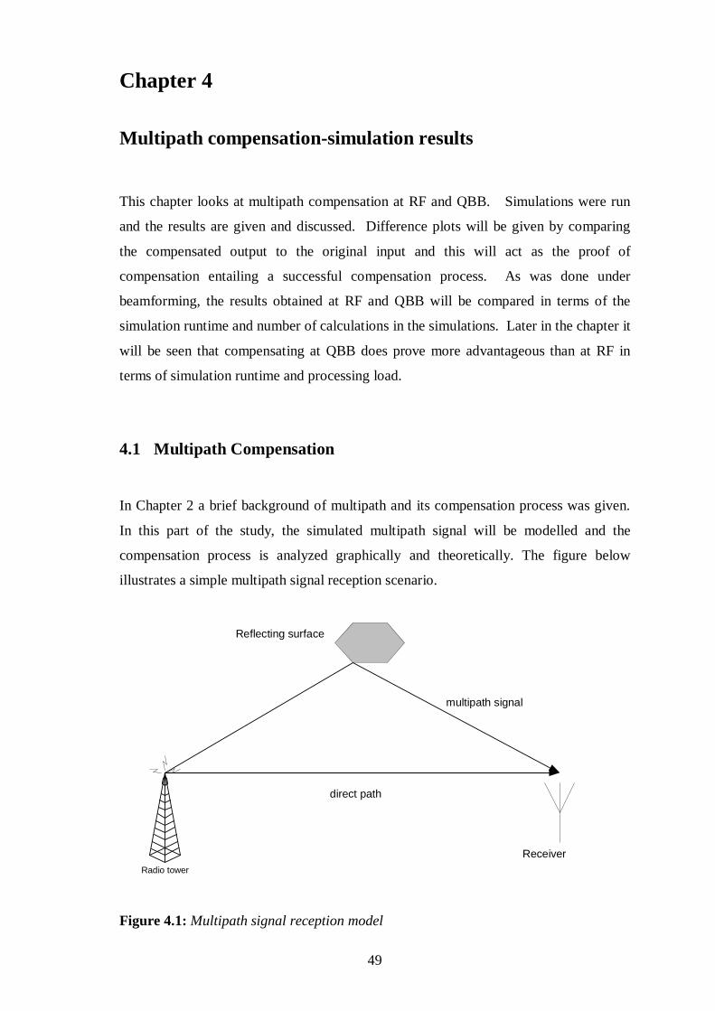
49

Chapter 4

Multipath compensation-simulation results This chapter looks at multipath compensation at RF and QBB. Simulations were run

and the results are given and discussed. Difference plots will be given by comparing

the compensated output to the original input and this will act as the proof of

compensation entailing a successful compensation process. As was done under

beamforming, the results obtained at RF and QBB will be compared in terms of the

simulation runtime and number of calculations in the simulations. Later in the chapter it

will be seen that compensating at QBB does prove more advantageous than at RF in

terms of simulation runtime and processing load.

4.1 Multipath Compensation

In Chapter 2 a brief background of multipath and its compensation process was given.

In this part of the study, the simulated multipath signal will be modelled and the

compensation process is analyzed graphically and theoretically. The figure below

illustrates a simple multipath signal reception scenario.

Radio tower

multipath signal

direct path

Receiver

Reflecting surface

Figure 4.1: Multipath signal reception model

50

CHAPTER 4 – MULTIPATH COMPENSATION: SIMULATION RESULTS

In Figure 4.1 on the previous page, it is seen that the antenna at the destination receives

two signals namely the direct-path and delayed signal. For analysis purposes, we will

restrict the number of multipath signals to one. Before carrying out the analysis, there is

need to model the multipath signal and correct compensator which will eliminate the

multipath effects and resulting in the required direct-path signal output.

Multipath signal modelling

The multipath channel H comprises a component of the direct path signal and the

delayed multipath signal. The multipath signal is undesired and hence the need for us to

compensate for its presence and thus eliminate its effects. The goal of the compensation

is to recreate the characteristics of the original signal just as it was before the delayed

signal was introduced. This requires us to have knowledge of the characteristics of the

channel (i.e. frequency or impulse response) in order to determine the correct

compensator denoted as Hc. It is well known that convolving in the time domain is

equivalent to multiplication in the frequency domain and vice-versa [3]. This means

that we can equally have a model for the multipath signal by convolving in the time

domain. However, using the time domain method, there are some important limitations

in that we are restricted to discrete sample delays ‘nTs’ and thus the compensation

process is limited by the fact that we cannot carry out downsampling beyond a point

where the echo does not lie on a sample instant anymore and this has much to do with

the echo positioning. The multipath channel modelling was done in the frequency

domain and hence the signal compensation equally took place in the frequency domain.

The famous time delay Fourier transform [3, 5] does facilitate for operating in the

frequency domain. This is given below.

( ) ( )jf t F e ωττ ω −− ↔ (4.1)

Therefore, the received signal as already mentioned in Chapter 2 has the direct and

multipath components in it and so the multipath channel ‘H’ will be given as

H= 1+ e-jωτ (4.2)

51


It should be noted that in this case, τ is not restricted to nTs. The modelling of the

multipath signal is thus done in the frequency domain and hence it is required that an

equivalent domain is used in the compensation process. The QAM/FM modulated

signal direct path signal is ‘zero padded ‘and its FFT [5] is taken. This facilitates the

circular convolution in the frequency domain whose equivalent is linear convolution in

the time domain [24].

Similarly, the channel response is zero padded and followed by the FFT so as to have

its frequency domain equivalent in readiness for the circular convolution. After

carrying out the circular convolution, the resulting signal is transformed back to the

time domain by taking its IFFT. The signal at hand is now a real multipath signal in

readiness for analysis. The analysis then moves to the receiving end where the

compensation takes place. Here, the received signal was transformed back to the

frequency domain by taking the FFT and this was done so as to compensate in the

frequency domain.

4.2 Multipath Compensation:–Radio Frequency

RF multipath compensation represents a traditional method of compensating for

unwanted multipath signal effects. In this study, we assumed noiseless channels since,

we are basically showing the possibility of compensating for multipath at RF and QBB

with the latter being the new method and showing the expected benefits of

compensating at quadrature baseband.


The theoretical analysis for the multipath compensation at RF is given below. In this

part of the study, QAM and FM modulation were analyzed.

The direct path signal is represented asdx . The received multipath signal being the sum

of the direct path and its delayed echo is thus given as

( )mp d dx x kx t τ= + − (4.3)

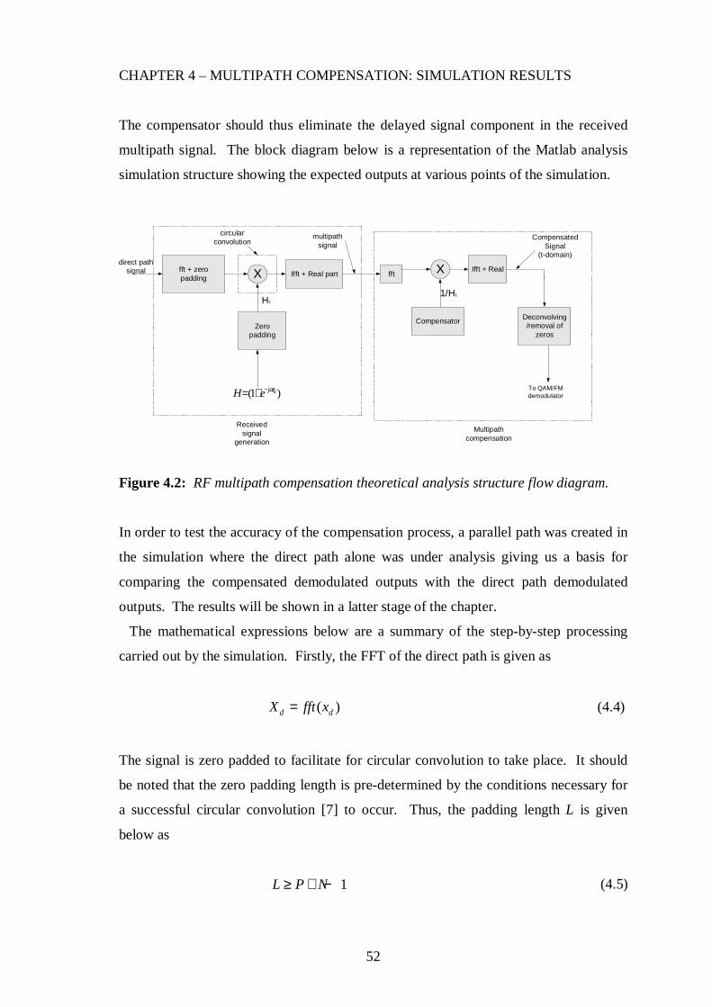
52


The compensator should thus eliminate the delayed signal component in the received

multipath signal. The block diagram below is a representation of the Matlab analysis

simulation structure showing the expected outputs at various points of the simulation.

fft + zeropadding X Ifft + Real part

Zeropadding

direct pathsignal fft X Ifft + Real

Deconvolving/removal of

zeros

H1

Receivedsignal

generation

Multipathcompensation

multipathsignal

1/H1

circularconvolution

CompensatedSignal

(t-domain)

To QAM/FMdemodulator(1 )dj tH e ω−= +

Compensator

Figure 4.2: RF multipath compensation theoretical analysis structure flow diagram.

In order to test the accuracy of the compensation process, a parallel path was created in

the simulation where the direct path alone was under analysis giving us a basis for

comparing the compensated demodulated outputs with the direct path demodulated

outputs. The results will be shown in a latter stage of the chapter.

The mathematical expressions below are a summary of the step-by-step processing

carried out by the simulation. Firstly, the FFT of the direct path is given as

( )d dX fft x= (4.4)

The signal is zero padded to facilitate for circular convolution to take place. It should

be noted that the zero padding length is pre-determined by the conditions necessary for

a successful circular convolution [7] to occur. Thus, the padding length L is given

below as

1L P N≥ + − (4.5)

53


where P is the length of the direct path signal and N the length of the channel impulse

response [24]. Therefore, the frequency domain multipath signal Xmp which now has a

length twice that of xd is given as

mp dX X H= (4.6)

Taking the real part of the IFFT of Xmp gets rid of the small imaginary part due to

limited numerical accuracy resulting in the received multipath signal expressed below

as

Re[ ( )]rmp mpx ifft X= (4.7)

where xrmp represents the received multipath signal. As mentioned earlier, the

compensation will take place in the frequency domain and hence the need to convert the

received signal xrmp to the frequency domain before compensation can take place. Now

Hc=H -1 and H being a frequency domain vector means the compensator is thus in the

frequency domain and thus the compensation can now proceed, having achieved the

same domain of operation for the received signal and compensator.

rc rmp cX X H= (4.8)

where Xrc represents the compensated received signal in the frequency domain. The

time domain equivalent of the compensated signal is given below as

Re[ ( )]rc rcx ifft X= (4.9)

The original size of the compensated signal is achieved by removing the padded zeros.

The original modulated signal is thus retrieved and the demodulated outputs achieved

by carrying out QAM/FM demodulation resulting in the compensated demodulated

output xrcd .

54


4.3 Multipath compensation:- Quadrature baseband

The analysis moves down to quadrature baseband where the compensation will now

take place. This in itself presents a major advantage of operating at lower sampling

frequencies added on to the fact that operating at baseband also facilitates for

downsampling which further reduces the operating frequency of the compensation

process.

Theoretical analysis:-QBB

The input parameters used for this analysis are the same as those of their RF

counterparts. This implies that we have the same signal parameters like amplitude,

angular velocity etc. Similarly we have the same initial sampling rate (fs) and the local

oscillator frequency used in the complex down-mixing process is coherent with the

carrier frequency.

Upon analysis of the results, a decisive conclusion was to be reached about the

possibility of compensating at QBB accompanied by the various benefits that come with

working at QBB frequencies. Some of the advantages of working at baseband

frequencies are attributed to the ease of handling of baseband digital signals by software

defined radios and hence resulting in the immense benefits of SDR technology being

utilized [16]. The expressions for the direct path and multipath signals have already

modelled under the RF theoretical analysis. And thus the analysis moves on to the

receiver where it is required that we compensate at QBB. The received signal ‘xrmp’ is

down-mixed and lowpass filtered so as to generate its QBB equivalent.

[ ]cjw trmpqbb rmp LPFx x e−= (4.10)

where xrmpqbb represents the QBB version of the received multipath signal. The block

diagram on the next page is a representation of the Matlab analysis simulation structure

showing the expected outputs at various points of the simulation. The figure on the next

page summarises the theoretical analysis.

55


Direct path signal FFT + zeropadding

Zeropadding

Ifft + Real partX X LPF FFT X

X

ifft

Deconvolution/removal of

zeros

LPF + FFT

Received signalmodelling Multipath compensation

Receivedmultipath signal

QBB signal

(1 )dj te ω−+

cj te ω−

Downsamplingtakes place here

Compensator

circular convolution

mixed-down signal

H=

H1

To QAM/FM QBBdemodulator

Hc=1/H1

Figure 4.3: QBB multipath compensation theoretical analysis flow structure.

The compensation is thus done at QBB as required by the study. The simulation results

will verify the compensation process illustrated theoretically by the figure above. Upon

generating the QBB equivalent of the multipath signal, down sampling is also carried

out. The quadrature baseband signal is downsampled by a factor ‘n’ whose value is

restricted to the point where there is no aliasing in the spectrum. What this statement

implies is that one can only downsample up to a certain point and that point is where

aliasing begins to take place. It is a well known factor that aliasing is an undesirable

situation and thus it has to be avoided at all costs. The downsampled signal is given in

Matlab as

(1: : )rqbbdsx xrqbb n end= (4.11)

where xqrbbds represents the downsampled QBB signal. At this stage, the analysis

focuses on the compensation process where it was required to compensate for the

multipath effects. Now, in order to compensate for multipath at this stage, it is required

to shift the compensation down to baseband because the signal now sits at baseband.

This in itself is an added advantage of compensating at QBB because this takes place at

much lower frequencies unlike for the RF situation. The compensator should equally be

56


downsampled before the compensation can take place. The QBB downsampled

compensator is denoted as Hcds. The compensation can now take place and this is done

by multiplying Hcds with the FFT of xrbbds denoted as Xrqbbds. This is shown below as

rc rqbbds cdsX X H= (4.12)

where Xrc denotes the compensated signal in the frequency domain whose time domain

equivalent is given in Equation 4.13 below. The padded zeros should be eliminated at

this stage. There is need to take into consideration the fact that the signal length has

reduced by a factor ‘n’ and hence this should not be overlooked when removing the

padded zeros. The IFFT of Xrc is given below as

( )rc rcx ifft X= (4.13)

The signal xrc is then demodulated and is denoted as xrcd. In the simulations that follow,

a parallel analysis is run for the direct path signal which is demodulated and compared

with the compensated output so as to test the accuracy of the compensation process.

The demodulated output from the parallel analysis is denoted as xrd. The next section of

the chapter gives the RF simulation results.

57


4.4 Simulation Results:–QAM RF compensation

The figures below are the results obtained from the multipath compensation simulation

at RF. The sampling frequency fs used was 4000Hz and x1 and x2 shown in Figure

4.4(a) are the unmodulated inputs of the QAM direct path signal shown in Figure 4.4(b).

As mentioned under the RF theoretical analysis, the zero padding during the multipath

signal generation doubles the signal length and this is evidenced in Figure 4.4(c).

Compensating for multipath as outlined in the theoretical analysis results in the output

shown in Figure 4.4(d). It can be seen here that the QAM signal has been retrieved and

the multipath effects compensated for. The demodulated outputs and difference plot

should further consolidate the accuracy of the compensation.

0 100 200 300 400 500 600 700 800 900 1000-1

-0.8

-0.6

-0.4

-0.2

0

0.2

0.4

0.6

0.8

1unmodulated inputs

samples

ampl

itude

x1

x2

0 100 200 300 400 500 600 700 800 900 1000-1

-0.8

-0.6

-0.4

-0.2

0

0.2

0.4

0.6

0.8

1QAM modulated signal

samples

ampl

itude

0 200 400 600 800 1000 1200 1400 1600 1800 2000-2

-1.5

-1

-0.5

0

0.5

1

1.5

2received signal

samples

ampl

itude

(c)

0 100 200 300 400 500 600 700 800 900 1000-1

-0.8

-0.6

-0.4

-0.2

0

0.2

0.4

0.6

0.8

1received compensated QAM modulated signal

samples

ampl

itude

(d)

(a) (b)padded zeros

Figure 4.4: Simulation results (a) Unmodulated inputs:- these represent the inphase

and quadrature phase inputs of the QAM signal (b) QAM modulated signal (c)

Received signal:-the last 1020 samples consist of padded zeros (d) Compensated signal.

58


The figures below show the demodulated outputs and difference plot.

(a) (b)

(c)

0 200 400 600 800 1000 1200-1

-0.8

-0.6

-0.4

-0.2

0

0.2

0.4

0.6

0.8

1demodulated outputs from direct path signal only

samples

ampl

itude

demodulated output xd1


0 200 400 600 800 1000 1200-1

-0.8

-0.6

-0.4

-0.2

0

0.2

0.4

0.6

0.8

1demodulated outputs

samples

ampl

itude

demodulated output x1

demodulated output x2

0 100 200 300 400 500 600 700 800 900 1000

-2.5

-2

-1.5

-1

-0.5

0

0.5

1

1.5

2

2.5

x 10-15 Difference/error plot

samples

ampl

itude

xd1-x1

xd2-x2

Figure 4.5: Simulation results. (a) Demodulated output after compensation (b)

Demodulated output from direct path (c) Difference plot between direct path and

multipath compensated demodulated outputs.

The difference plot clearly shows a very small and insignificant error. This proves that

the compensation was accurate and successful. A look at the spectral changes in the

following section of the chapter further consolidates the proof of a successful

compensation.

59


Spectral Analysis of results

The figures below represent the magnitude spectra of the signals resulting from the RF

multipath compensation simulation. The spectral changes that took place are analyzed

in order to have proof of the compensation from the spectral point of view.

0 500 1000 1500 2000 2500 3000 3500 40000

50

100

150

200

250

300magnitude spectrum of modulated signal

frequency(Hz)

mag

nitu

de

0 500 1000 1500 2000 2500 3000 3500 40000

100

200

300

400

500

600magnitude spectrum received signal

frequency(Hz)

mag

nitu

de

(b)(a)

Figure 4.6: Magnitude spectrum of (a) Modulated input signal (b) Received signal

The Figure 4.6 (a) above illustrates the magnitude spectrum of the QAM modulated

signal before multipath and Figure 4.6(b) represents the magnitude spectrum of the

received signal. The multipath component increased the magnitude of the spectral

content of the signal as can be seen. Figure 4.7 below shows that the compensation

process restored the original spectrum of the signal.

0 500 1000 1500 2000 2500 3000 3500 40000

50

100

150

200

250

300magnitude spectrum of compensated signal

frequency(Hz)

mag

nitu

de

(c)

Figure 4.7: Magnitude spectrum of compensated signal.

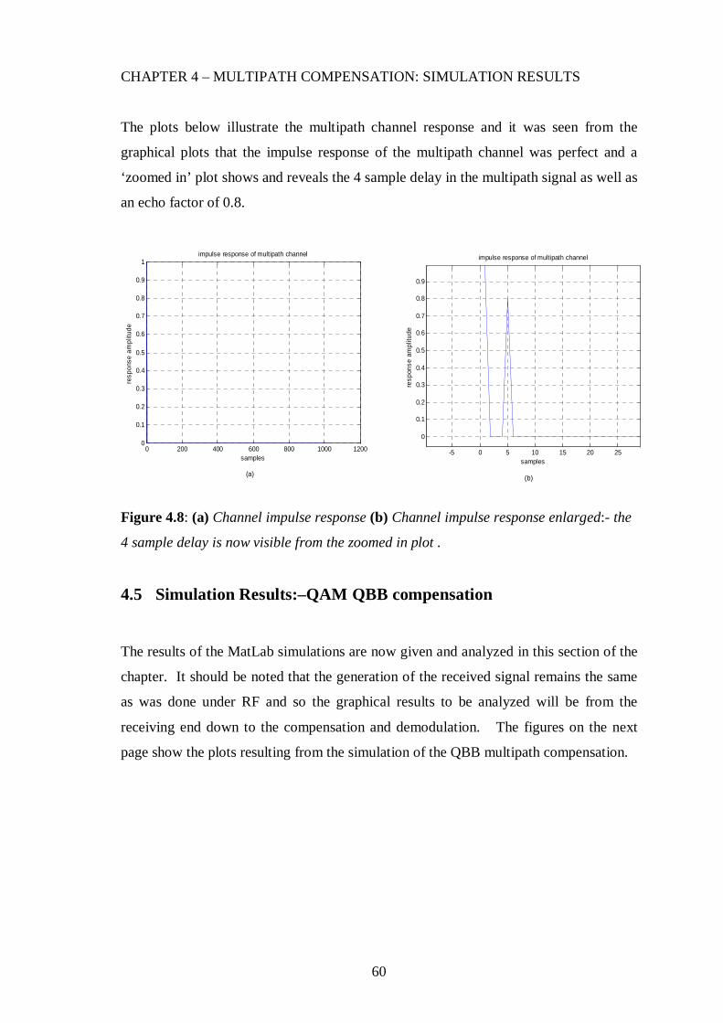
60


The plots below illustrate the multipath channel response and it was seen from the

graphical plots that the impulse response of the multipath channel was perfect and a

‘zoomed in’ plot shows and reveals the 4 sample delay in the multipath signal as well as

an echo factor of 0.8.

0 200 400 600 800 1000 12000

0.1

0.2

0.3

0.4

0.5

0.6

0.7

0.8

0.9

1impulse response of multipath channel

samples

resp

onse

am

plitu

de

-5 0 5 10 15 20 25

0

0.1

0.2

0.3

0.4

0.5

0.6

0.7

0.8

0.9

impulse response of multipath channel

samples

resp

onse

am

plitu

de

(b)(a)

Figure 4.8: (a) Channel impulse response (b) Channel impulse response enlarged:- the

4 sample delay is now visible from the zoomed in plot .

4.5 Simulation Results:–QAM QBB compensation

The results of the MatLab simulations are now given and analyzed in this section of the

chapter. It should be noted that the generation of the received signal remains the same

as was done under RF and so the graphical results to be analyzed will be from the

receiving end down to the compensation and demodulation. The figures on the next

page show the plots resulting from the simulation of the QBB multipath compensation.

61


-1.5 -1 -0.5 0 0.5 1 1.5-1.5

-1

-0.5

0

0.5

1

1.5received QAM modulated down-mixed signal

real part

imag

inar

y pa

rt

(a) (b)

-2 -1.5 -1 -0.5 0 0.5 1 1.5 2-2

-1.5

-1

-0.5

0

0.5

1

1.5

2received QAM QBB signal

real part

imag

inar

y pa

rt

Figure 4.9: Simulation results (a) Down-mixed received signal (b) QBB received signal

before compensation..

The figures below show the QBB signal after compensation and the demodulated

output. It is seen that the original inputs were successfully retrieved from the multipath

signal.

-1 -0.8 -0.6 -0.4 -0.2 0 0.2 0.4 0.6 0.8 1-1

-0.8

-0.6

-0.4

-0.2

0

0.2

0.4

0.6

0.8

1compensated QBB signal

real part

imag

inar

y pa

rt

(d)

0 50 100 150 200 250-1

-0.8

-0.6

-0.4

-0.2

0

0.2

0.4

0.6

0.8

1compensated received QBB demodulated signal

samples

ampl

itude

demodulated output y1demodulated output y2

(b)

Figure 4.10: (a) QBB signal after compensation (b) Demodulated compensated output.

The compensated signal had the padded zeros, that were introduced in the generation

stage, removed, and the original signal length was thus restored. The signal length was

reduced by the downsampling factor ‘n’ and in this particular case, the demodulated

signal outputs have a length of 256 samples the due to the downsampling factor being

equal to 4. The figures on the next page show the demodulated outputs from the direct

path signal demodulation for comparison purposes.

62


A difference plot is also given to further verify the compensation accuracy.

0 50 100 150 200 250-1

-0.8

-0.6

-0.4

-0.2

0

0.2

0.4

0.6

0.8

1demodulated signal from direct path signal only

samples

ampl

itude

xrd1

xrd2

(a) (b)

0 100 200 300 400 500 600 700 800 900 1000

-2

-1

0

1

2

3x 10

-14 Difference/Error plot

samples

ampl

itude

Figure 4.11: (a) Direct path demodulated output:-forms the basis for comparison so as

to determine the preciseness of the compensation process. (b) Difference/error plot:-

indicates that the compensation was successful despite the error being slightly higher

than for the previous analyses.

4.5.1 Spectral Analysis

The spectral changes and results of the QBB compensation process are shown in the

figures on the next page. The spectral changes do elaborate more on the compensation

process and also show that the compensation process took place at quadrature baseband.

63


0 500 1000 1500 2000 2500 3000 3500 40000

50

100

150

200

250

300

350

400

450magnitude spectrum of received multipath signal

frequency(Hz)

mag

nitu

de

0 500 1000 1500 2000 2500 3000 3500 40000

50

100

150

200

250

300

350

400

450magnitude spectrum of down-mixed signal

frequency(Hz)

mag

nitu

de

(b)(a)

0 500 1000 1500 2000 2500 3000 3500 40000

100

200

300

400

500

600

700

800


frequency(Hz)

mag

nitu

de

0 100 200 300 400 500 600 700 800 900 10000

20

40

60

80

100

120

140magnitude spectrum of compensated received signal

frequency(Hz)

mag

nitu

de

(d)(c)

Figure 4.12: Magnitude spectra plots.(a) Received signal (b) Down-mixed signal (c)

QBB downsampled signal (d) QBB downsampled compensated signal.

The conversion process from RF to QBB has been outlined in earlier chapters. The

down conversion of the sample rate is an important part of digital signal processing.

The compensated signal spectrum is shown at quadrature baseband in Figure 4.12(d).

4.6 Simulation results:– FM RF compensation

This section continues the multipath compensation analysis but looks at FM modulated

signals. The simulation results are given and discussed. It should be noted that the

spectral analysis done in the previous QAM study does suffice in explaining the

changes that will take place in under the FM analysis and hence referring back does

suffice in explaining the current analysis so as to avoid repetition. The principles of the

64


compensation process carried out under QAM compensation remain the same under FM

and therefore, it suffices to go straight to the actual simulation results. The figures

below illustrate the simulation results obtained for compensation at RF. The sampling

frequency used was 4000Hz and the number of samples was 1024. As done in the

previous simulations, the parameter conditions used for the RF simulations are the same

as those used for the QBB simulations so as to have a fair comparison between the two.

0 100 200 300 400 500 600 700 800 900 1000-1

-0.8

-0.6

-0.4

-0.2

0

0.2

0.4

0.6

0.8

1compensated received signal

samples

ampl

itude

(d)

(a) (b)

0 200 400 600 800 1000 1200 1400 1600 1800 2000-2

-1.5

-1

-0.5

0

0.5

1

1.5

2recieved signal

samples

am

plit

ud

e

(c)

0 100 200 300 400 500 600 700 800 900 1000-1

-0.8

-0.6

-0.4

-0.2

0

0.2

0.4

0.6

0.8

1modulating input signal

samples

ampl

itude

0 100 200 300 400 500 600 700 800 900 1000-1

-0.8

-0.6

-0.4

-0.2

0

0.2

0.4

0.6

0.8

1direct path signal

samples

ampl

itude

Figure 4.13: Simulation results. (a) modulating signal (b) FM modulated input signal

(c) Received signal:-comprises the actual signal with padded zeros (d) Compensated

signal: the original signal is restored.

From Figure 4.13(c) it is seen that the signal has 2048 samples of which the last 1020

are zeros and this is due to the zero padding that was done when carrying out the

circular convolution. The delay in the FM analysis was 4 samples too and so the

received signal had non-zero values up to 1028 samples. The compensation process

effectively compensated for the multipath effects and therefore, the compensated signal

65


had non-zero values up to 1024 and the remaining zeros were eliminated to retain the

original input signal length. The figures on the next page show the demodulated output

resulting from the compensated signal and the direct path signal only and the difference

plot between the demodulated compensated output and the direct path demodulated

output.

0 100 200 300 400 500 600 700 800 900 1000-1

-0.8

-0.6

-0.4

-0.2

0

0.2

0.4

0.6

0.8

1demodulated signal

samples

ampl

itude

0 100 200 300 400 500 600 700 800 900 1000-1

-0.8

-0.6

-0.4

-0.2

0

0.2

0.4

0.6

0.8


samples

ampl

itude

(b)(a)

(c)

0 100 200 300 400 500 600 700 800 900 1000

-3

-2

-1

0

1

2

x 10-14 Difference/Error plot

samples

ampl

itud

e

Figure 4.14: (a) Compensated signal demodulated output: the compensated modulated

output was demodulated and gives this signal output. The effectiveness or accuracy of

the compensation process remains to be tested by demodulating the direct path signal

with the same filter characteristics and compare the results. (b) Direct path signal

demodulated output: this signal output facilitates for measuring of the accuracy of the

compensation process by plotting its difference from the compensated demodulated out

put. (c) Difference/error plot: shows a successful compensation was done.

66


4.7 Simulation results:– FM QBB compensation

Here, we are again carrying out multipath compensation process but at QBB

frequencies. The multipath compensation is also done at much lower sampling rates

after carrying downsampling of the QBB received signal at baseband. The first four

figures below represent the received signal, down-mixed signal QBB signal before

compensation and after compensation. The FM modulated signal remains as given in

Figure 4.13(b) and is therefore not shown. Referring back to the QAM QBB

description of the above mentioned signals does suffice in describing the signals below

taking note however, that the modulation being considered is FM.

0 50 100 150 200 250-1

-0.8

-0.6

-0.4

-0.2

0

0.2

0.4

0.6

0.8

1demodulated compensated signal

samples

ampl

itude

(c)

0 50 100 150 200 250-1

-0.8

-0.6

-0.4

-0.2

0

0.2

0.4

0.6

0.8

1

demodulated signal from direct path signal only

samples

am

plit

ude

(d)

-2 -1.5 -1 -0.5 0 0.5 1 1.5 2-2

-1.5

-1

-0.5

0

0.5

1

1.5

2Received QBB signal

real axis

imag

inar

y ax

is

-1 -0.8 -0.6 -0.4 -0.2 0 0.2 0.4 0.6 0.8 1

-1

-0.8

-0.6

-0.4

-0.2

0

0.2

0.4

0.6

0.8

1

compensated received QBB signal

real axis

imag

ina

ry a

xis

(a)(b)

Figure 4.15: Simulation results (a) QBB signal before compensation.(b) Compensated

QBB signal. (c) Compensated demodulated output (d) Direct path demodulated output.

67


It is seen from Figure 4.15(c) and (d) that the direct path demodulated signal is similar

to the demodulated output from the compensated signal.

0 50 100 150 200 250

-2.5

-2

-1.5

-1

-0.5

0

0.5

1

1.5

x 10-3 Difference/error plot

samples

ampl

itude

Figure 4.16: Difference/error plot: shows that the compensation process was successful

with insignificant mismatches expected at some points of the plot.

The difference plot above does justify the accuracy and efficiency of the compensation.

The spectral changes are as seen under the QAM case and therefore the explanation

given earlier does suffice in explaining the expected spectral changes throughout the

FM QBB multipath compensation process. Therefore, it suffices to fairly conclude that

the multipath compensation has been successful and the error plot in itself serves as the

proof of compensation.

4.8 Benefits of compensating for multipath at QBB

Having run the simulations and analyzed the results, it is necessary to consolidate the

results by comparing the sample processing and sampling times as was done under

beamforming. The table on the next page summarises the sample processing at RF and

QBB for the multipath compensation simulation carried out for QAM modulation. The

sample processing was derived from the simulation code in the same way as was done

in the previous Chapter 3 for the AMDSB-SC RF/QBB simulations under beamforming

and is given in Appendix C which contains the simulation M-Files too.

68


For the simulated QBB case, the number of samples reduces after the downsampling

stage determined by the factor k.

Simulation Stages Radio Frequency Quadrature baseband(simulated)

Mixing down + QBB

+ Down sampling

____ 2N+2NLog22N

2N+2kN

Compensation

process

2N+ 2NLog22N

2N+ 2Nlog22N

2N+ N+ N

2kN+2kNLog22kN

2kN+2kNLog22kN

kN

Demodulation 2N + 2NLog2N+ N

2NLog2N + N

_______

Total sample

processing

10N+4NLog22N+

4NLog2N

2N+6kN+2NLog22N+

4kNLog22kN

Total sample

processing for

N=1024 and k=1/4

98304 37632

Table 4.1: Number of calculations at RF and QBB

The value of N was 1024 representing the number of samples with the downsampling

factor used for the simulation QBB case being equal to 4 (i.e. k=1/4). The sample

processing result shows that more processing was done at RF than QBB. The sub-

sampling done at QBB is the main reason for the reduction for the reduction in sample

processing at QBB. The runtime time for each simulation was measured as illustrated

earlier under beamforming. The simulation runtime comparisons given in the Table

below show that the processing at RF equally took longer than the processing at QBB

and this is due to the obvious reason that less samples were being processed for the

QBB simulation. Therefore, the sample processing results serve as the theoretical

verification of the actual simulation results. The table on the next page summarises the

simulation runtime and sample processing for the RF and QBB simulations carried out.

69



Multipath compensation Time in seconds Ratio Number of calculations Ratio

QAM 0.02715 0.01025 2.65 98304 37632 2.61

Table 4.2: Simulation runtime and number of calculations: RF/QBB ratio comparison.

It is seen from the table that the discrepancy between the simulation and theoretical

results is small (about 1.5%) and hence it suffices to say that the analysis carried out by

the simulations was correctly done. The analogue real life QBB method should result in

even further reduced calculations due to the fact that the real life situation assumes the

processing of the signals at QBB already. Thus from Table 4.1, the number of

calculations for the case at hand reduces to 10496 resulting in the ratio of the number of

calculations at RF to those at QBB being equal to

98304

9.3710496

rf

qbb

N

N= = (4.14)

Thus we see a bigger reduction in the number of calculations for the analogue QBB case

with the simulation processing time expected to follow suit. The limitation faced for the

FM case is also encountered here for reasons explained earlier under the beamforming

simulation result analysis. From the results obtained it is seen that compensating for

multipath at QBB reduced the amount of processing carried out as compared to the RF

case and consequently the simulation runtime was less for the latter which entails that

processing at QBB was thus faster.

70


4.9 Conclusion

The chapter illustrated that multipath compensation is possible at baseband frequencies

and there are benefits that come with operating at baseband which have been stressed

already. The study analysis did bring to light another added advantage: the

downsampling possibilities when operating at baseband. Therefore, latest baseband

technologies will be gaining on costs and reduced operation complexity by

implementing quadrature baseband multipath compensation. It was observed that the

analysis started with a much higher sampling rate and at baseband, the sampling rate

was reduced by a quarter and it should be noted that further reduction is possible and

the furthest point the downsampling can go is at the point where aliasing begins to

occur. However, it does suffice to say that QBB compensation surpasses RF

compensation in terms of operational advantages. Multipath does have remedies and

the traditional means of compensating for its effects have worked well over the years.

However, increasing technological awareness has given room for further research of

which Software defined radio technology stands out as the most prominent driving

factor. The study was able to carry out simulation analysis and it has been verified that

compensation at quadrature baseband can take place and indeed it comes with

significant processing advantages which would make it more preferable to radio

frequency compensation. Therefore, the study was worthwhile and relevant so as to

verify the possibility and effectiveness of quadrature baseband multipath compensation

for which we saw that we are able to downsample our signal during the analysis

facilitating for much lower sampling frequencies and hence reducing the complexity

[35] of the overall compensation process. The benefits are expected to pour down to

SDR technologies which currently make use of baseband processing.

71

Chapter 5 Doppler Shift compensation-Simulation results

This chapter briefly outlines the Doppler shift theorem. The Doppler shift

compensation process is also analyzed in general and simulation results from the

compensation process for the QAM and FM modulation schemes are given and

discussed. The proof of compensation is illustrated by the difference plot and this was

done for each simulation. The simulation runtimes and number of calculations show

how much more advantageous compensating for Doppler shift at QBB than at RF is. A

much bigger gain in terms of simulation runtime and number of calculations is expected

for the real life QBB scenario as will be shown from the benefits of working at QBB.

5.1 Doppler Shift

The Doppler effect refers to the change in frequency and wavelength of a signal as seen

by a receiver moving relative to the transmission source [25]. The overall Doppler

effect may therefore result from either motion of the source or motion of the receiver.

Each of these effects is analyzed separately. For signals requiring a medium, such as

light or gravity in specific relativity, only the relative difference in velocity between the

observer and the source is worth considering. The figure below illustrates the Doppler

effect.

TRX RX

TRX RX

(a) Approaching Targets

(b) receeding targets

Doppler shifted signal

Doppler shifted signal

Figure 5.1: Doppler Shift Model (a) Approaching Targets: result in a positive Doppler

shift frequency. (b) Receding targets: results in a negative Doppler shift.

72

CHAPTER 5 – DOPPLER SHIFT COMPENSATION: SIMULATION RESULTS

In Figure 5.1(a) on the previous page the transmitter and the receiver approach each

other resulting in a positive Doppler shift due to compression of the signal waveforms

resulting in a higher received frequency. This is also referred to as a positive Doppler

shift. In part Figure 5.1(b), the targets are receding from each other resulting in

expansion of the received signal waveforms which results in a lower received

frequency. This is referred to as a negative Doppler shift. Appendix B derives the

Doppler shift frequency for a slowly fluctuating target. For analysis purposes, the

Doppler shift used in the simulations was large enough so as to be able to see and

analyze the spectral changes taking place. This assumption is an exaggeration of the

real life situation in terms of the Doppler shift frequency size merely for analytical

purposes. The assumption entails frequency shifting and not frequency scaling for the

modeling of the Doppler signal.

5.2 Doppler shift model signal modeling

A Doppler signal can be modeled using frequency translation analysis in the time

domain. Therefore, in order to successfully model a Doppler signal in MatLab, we need

to fully understand the frequency translation or frequency shifting theorem [3].

Therefore, the next part of this section illustrates the frequency translation theorem in

detail. The Doppler signal in our case is assumed to have a higher frequency than the

original direct path signal and hence the transmitter and receiver are assumed to be

approaching each other. This part of the study aims to compensate for Doppler shift at

RF and compare and at QBB so as to show that it is equally possible to compensate for

Doppler shift at quadrature baseband as it is done at RF. The RF and QBB theoretical

analysis are given in the following sections of the chapter.

5.3 Theoretical analysis:- Doppler shift compensation at RF

Let xd represent the direct path signal. The Doppler shifted version of the signal thus is

given as

dj tdp dx x eω= (5.1)

It must be noted that the received signal must be real and hence, the resulting complex

signal from the multiplication above is transformed to a real signal. The Doppler

73


shifted signal is given below as

Re{[ ] }dpr dp FILTERx x= (5.2)

At the receiving end, it is required that the frequency shift caused by the Doppler effect

is compensated for by restoring the frequency spectrum to its original form. The

Doppler shift compensation analysis structure was illustrated by means of a flow

diagram in Chapter 2. Having modeled the Doppler shifted signal, it is thus required to

compensate for the Doppler shift using an appropriate compensator. Considering the

generation of the doppler signal model, it is seen that multiplication with dj te ω shifts the

direct path signal spectrum up by dω and so the compensator must be able to shift back

the frequency spectrum of the received signal by the same amount so as to return the

original frequency characteristics of the transmitted signal before the doppler effect

occurred.

Let h = dj te ω represent the Doppler shift channel and hc the compensator transfer

function both being in the time domain. It will be seen that in order to compensate for

the Doppler shift, the compensator has to undo the effects of the Doppler shift channel

on the direct path signal and therefore, the compensator turns out to be the inverse of the

Doppler shift channel. Thus we have:

Re[ ]dpr dx x h= (5.3)

Let xdprc represent the Doppler shift compensated received signal and h is related to hc

by the following expression;

1 1/c ch h h−= = (5.4)

Or

dj tch e ω−= (5.5)

Having formulated the compensator, we have our Doppler shift compensated signal

given as

dprc dpr cx x h= (5.6)

74


Therefore, the compensated signal is the output of the multiplication between the

received Doppler shifted signal and the compensator hc and it is seen that the

compensation takes place in the time domain. At this stage the resulting signal is still

complex and hence the need to convert it to a real signal by filtering the higher

frequency component and taking the real part as was done in the generation of the

doppler shift signal. This is given below as

Re{[ ] }rc dprc FILTERx x= (5.7)

At this stage, the compensated signal is ready for demodulation so as to retrieve the

message signal. QAM/FM demodulation is then carried out resulting in the

compensated demodulated output. The figure below summarizes the theoretical

analysis discussed above.

Doppler channel 'H'Filter + ifft+ real part Compensator 'hc'

1/Filter+ ifft+ Real Part

Direct path signal

dj te ω dj teω

To demodulator

dprx

rcx

dprcx

dpx

Figure 5.2: Theoretical analysis general structure.

The generation of the Doppler shift signal model remains the same as in the previous

chapter with the difference being the compensation process. The aim of the study

entails compensating at quadrature baseband and hence we will justify its possibility

and compare the results with those from the RF process so as to show the accuracy of

the compensation process.

75


5.4 Theoretical analysis:- Doppler shift compensation at QBB

The received signal xdpr is mixed down at the receiver giving us the received down-

mixed signal given as

cj tdprdm dprx x e ω−= (5.8)

where xdprdm denotes the Doppler received down-mixed signal. The down-mixed signal

is then lowpass filtered resulting in the QBB signal xdprqbb.

[ ]dprqbb dprdm LPFx x= (5.9)

The Doppler QBB Doppler compensation process does allow for downsampling to be

incorporated and in this case it is implemented at this stage. The downsampling is

implemented as done in previous analysis. This should equally be done for the

compensator.

(1: : )dprqbbds dprqbbx x n end= and (1: : )cds ch h n end= (5.10)

where xdprqbbds represents the quadrature baseband Doppler shifted down sampled signal

and hcds the downsampled compensator. The compensation then proceeds as shown in

below:

rc dprqbbds cdsx x h= (5.11)

It will be interesting to note that the same compensator used at RF is used at QBB.

However, QBB provides even further advantages in that there is no need to carry out

any further filtering unlike in the RF process so as to have our real demodulated output

signals. This will be seen from the simulation results. This is in itself a big advantage

of the QBB Doppler shift compensation process because the number of processing

stages will reduce which in turn reflects in reduced costs and complexity of equipment.

Demodulation then follows resulting in the demodulated outputs.

76


The figure below summarizes the theoretical analysis showing the expected signals at

different points of the analysis.

Doppler Channel 'H' LPF+ifft+Real

LPF+ifft+downsampling

Downsampling ofcompensator

Compensator'Hc'

X

Direct path signal

dj teω

dj te ω−

To QBB demodulator

X

cj te ω−

dpx

dprx dprdmx

dprqbbdsx

cdsh

r cx

Figure 5.3: Theoretical analysis block diagram for compensation at QBB. The signal

outputs at various points of the analysis are given.

77


5.5 Simulation Results:- QAM RF compensation

The figures below show the simulation results obtained for the RF Doppler shift

compensation. The sampling frequency used was 4000Hz and the number of samples

was 1024.

0 100 200 300 400 500 600 700 800 900 1000-1

-0.8

-0.6

-0.4

-0.2

0

0.2

0.4

0.6

0.8

1received QAM signal

samples

ampl

itude

0 100 200 300 400 500 600 700 800 900 1000-1.5

-1

-0.5

0

0.5

1

1.5Received doppler shift signal

samples

ampl

itude

(b)

0 100 200 300 400 500 600 700 800 900 1000-1

-0.8

-0.6

-0.4

-0.2

0

0.2

0.4

0.6

0.8


samples

mag

nitu

de

(c)

0 100 200 300 400 500 600 700 800 900 1000-1

-0.8

-0.6

-0.4

-0.2

0

0.2

0.4

0.6

0.8

1compensated demodulated signal

samples

ampl

itude

demodulated output xrcd1


(d)

(a)

Figure 5.4: (a) QAM direct path signal (b) QAM doppler shifted signal (c)

Compensated output signal (d) Demodulated compensated output signal.

From the plots given above, it is seen in figure 5.4(b) that the Doppler shift caused a

change in the received signal amplitude. The compensation process retrieved the

original direct path signal from the Doppler shifted signal as shown in figure 5.4(c).

The demodulation then followed resulting in the demodulated outputs denoted as xrcd1

and xrcd2 in Figure 5.4(d). The proof of an accurate compensation process was given by

the difference plot which according to Figure 5.5 (b) on the next page shows a

78


successful and accurate compensation process.

0 100 200 300 400 500 600 700 800 900 1000-1

-0.8

-0.6

-0.4

-0.2

0

0.2

0.4

0.6

0.8

1demodulated outputs from direct path signal only

samples

ampl

itude



(a)

0 100 200 300 400 500 600 700 800 900 1000-0.02

-0.015

-0.01

-0.005

0

0.005

0.01

0.015

0.02Difference/error plot

samples

ampl

itude

xd1-xrcd1

xd2-xrcd2

(b)

Figure 5.5: (a) Direct path demodulated output:- the inphase and quadrature phase

demodulated outputs are denoted as xd1 and xd2 respectively. (b) Difference plot:-

shows that the compensation was with minimal error.

Spectral analysis:- RF

The spectral analysis of the frequency spectral changes taking place in the whole

compensation process is given and discussed in this part of the chapter. Figures 5.6 (a),

and (b) below represent the spectral changes from the QAM signal down to the Doppler

shifted signal model.

0 500 1000 1500 2000 2500 3000 3500 40000

50

100

150

200

250

300magnitude spectrum of modulated signal

frequency(Hz)

mag

nitu

de

(a)

0 500 1000 1500 2000 2500 3000 3500 40000

50

100

150

200

250

300unfiltered magnitude spectrum of filtered spectrum for doppler shift signal

frequency(Hz)

mag

nitu

de

(b)

Figure 5.6: (a) QAM direct path signal spectrum (b) Frequency shifted QAM signal.

79


The direct path signal was multiplied with dj te ω which shifted the spectrum up by ωd

which represents the Doppler shift. However, it is seen that this is not a true model of a

typical Doppler spectrum because the spectrum is reflective of a complex signal and

therefore, we have to transform this spectrum into a real Doppler shift signal spectrum.

This is done by filtering out the spectral component that sits at 3100Hz and then taking

the real part of the remaining component so that they eventually sit at 1100Hz and

2900Hz so as to have a real Doppler shifted signal spectrum. The Doppler shift

frequency has been exaggerated for analytical purposes so as to be able to see the

spectral changes clearly. In reality, this shift is much smaller but significant enough to

cause reasonable signal distortions. Figure 5.7(a) below illustrates the filtered part of

our signal spectrum which leaves the component at 1100Hz and taking the real part

results in the symmetrical spectrum shown in Figure 5.7(b) which is reflective of a true

Doppler shifted signal model.

0 500 1000 1500 2000 2500 3000 3500 40000

50

100

150

200

250

300filtered magnitude spectrum of filtered for doppler shift signal

frequency(Hz)

mag

nitu

de

0 500 1000 1500 2000 2500 3000 3500 40000

50

100

150

200

250

300magnitude spectrum of doppler shift signal

frequency(Hz)

mag

nitu

de

(a)(b)

Figure 5.7: Spectral plots.(a) Filtered signal spectrum:- this is done to create a spectral

representation of a real doppler shifted signal. (b) Doppler shift signal spectrum:- the

Doppler shifted signal spectrum is even and hence it is now representative of a real

Doppler shifted signal.

Having seen the Doppler shifted signal spectrum the analysis focuses on the

compensation and aims to verify whether the original signal spectrum is retained by the

compensation process. The theoretical analysis did explain the compensation process

and the graphical simulation results do verify the theoretical expectations. In Figure

80


5.8(a) below, it is seen that that the compensator managed to successfully shift down the

lower frequency component of the Doppler shifted signal spectrum to 1000Hz with the

higher frequency component moving down to 2800Hz. At this stage, we have a

complex signal output. Therefore, the filtering process that occurred earlier is repeated

as this stage so as to have a real compensated signal output in readiness for the

demodulation process. Thus the 2800Hz component was filtered out as shown in Figure

5.8(b) and taking the real part results in the Doppler shift compensated signal spectrum

in Figure 5.8(c). This is a real signal spectrum due to its symmetrical properties. A

comparison between the compensated signal spectrum and original signal spectrum

shows that the original spectrum was restored. This further verifies the accuracy of the

compensation process carried out and the analysis in the next section looks at the

quadrature baseband way of compensating for Doppler shift in a signal.

0 500 1000 1500 2000 2500 3000 3500 40000

50

100

150

200

250

300magnitude spectrum of compensated (before filtering)doppler shift signal

frequency(Hz)

mag

nitu

de

(a)

0 500 1000 1500 2000 2500 3000 3500 40000

50

100

150

200

250

300magnitude spectrum of filtered compensated doppler shift signal

frequency(Hz)

mag

nitu

de

(b)

0 500 1000 1500 2000 2500 3000 3500 40000

50

100

150

200

250


samples

ampl

itude

(c)

Figure 5.8 Magnitude spectra plots (a) Compensated complex signal spectrum (b)

Filtered compensated signal spectrum (c) Real compensated signal spectrum: it is seen

that the original spectrum has been restored.

81


5.6 Simulation Results:- QAM QBB compensation

The simulation analysis results are given and discussed below. The same parameters

used for the RF simulation were used for the QBB simulation too.

-1.5 -1 -0.5 0 0.5 1 1.5-1.5

-1

-0.5

0

0.5

1

1.5received QAM modulated QBB s ignal

real part

imag

ina

ry p

art

(a)

-1.5 -1 -0.5 0 0.5 1 1.5-1.5

-1

-0.5

0

0.5

1

1.5compensated QBB signal

real part

imag

inar

y pa

rt

(b)

0 50 100 150 200 250 300 350 400 450 500-1

-0.8

-0.6

-0.4

-0.2

0

0.2

0.4

0.6

0.8


samples

ampl

itude



(c)

0 50 100 150 200 250 300 350 400 450 500-1

-0.8

-0.6

-0.4

-0.2

0

0.2

0.4

0.6

0.8

1demodulated signal outputs from direct path signal only

samples

ampl

itude

xrd1

xrd2

(d)

Figure 5.9: Simulation plots. (a) QBB received signal (b) Compensated QBB signal (c)

compensated demodulated output. (d) Direct path demodulated output.

Figure 5.9(a) represents the quadrature baseband version of the received signal. The

signal was then downsampled by a factor of ‘2’ resulting in a 2-fold sample reduction

from 1024 to 512. The compensator is downsampled to so as to adequately compensate

for the Doppler shift in the downsampled QBB received signal. Thus, sample

processing is reduced for the QBB case and this could translate to a much faster

operating speed or less operating time as will be shown in the concluding part of the

chapter. The compensation then followed resulting in the compensated QBB signal in

82


Figure 5.9(b) on the previous page. At this stage, it is interesting to note that there is no

need for any filtering so as to come up with a real doppler shift compensated signal

spectrum as was done under the RF Doppler compensation analysis because the signal

sits at QBB and QBB demodulation is able to retrieve the original input from the

complex QBB signal spectrum. This further entails reduced processing under this the

QBB and hence presents a significant advantage of this method of Doppler

compensation. Below is shown the difference plot resulting from a numerical

comparison between the compensated demodulated output in Figure 5.9 (c) and the

direct path demodulated output. It is seen that again, the compensation was a success.

0 50 100 150 200 250 300 350 400 450 500

-0.015

-0.01

-0.005

0

0.005

0.01

0.015

0.02

Difference/error plot

samples

ampl

itude

xrd1-xrcd1

xrd2-xrcd2

Figure 5.10: Difference plot: shows the numerical difference between the direct- path

demodulated signal and the compensated demodulated output.

Spectral analysis:- QBB

Figure 5.11 on the next page illustrates the spectral changes taking place for under the

QBB analysis process. Figure 5.11(a) represents the Doppler shifted signal spectrum.

Figure 5.11(b) shows the spectral components shifted down after the down-mixing

process and converted to QBB by lowpass filtering resulting in the spectrum shown in

Figure 5.11(c). It is seen that the number of samples has reduced by a factor of 2 due to

the reduction in the sampling rate by a similar factor. Figure 5.11(d) shows the

compensated signal spectrum plotted in terms of the samples so as to show the sample

reduction that took place. It is also seen from the figure that the Doppler shift has been

eliminated hence restoring the original spectrum which is now at quadrature baseband

which provides evidence of a successful compensation process.

83


0 50 100 150 200 250 300 350 400 450 5000

50

100

150

200

250


samples

mag

nitu

de

(d)

0 500 1000 1500 2000 2500 3000 3500 40000

50

100

150

200

250

300magnitude spectrum of QAM recieved down-mixed signal

frequency(Hz)

mag

nitu

de

(b)

0 50 100 150 200 250 300 350 400 450 5000

50

100

150

200

250

300magnitude spectrum of QAM recieved QBB signal

samples

mag

nitu

de

0 500 1000 1500 2000 2500 3000 3500 40000

50

100

150

200

250

300magnitude spectrum of doppler shift signal

frequency(Hz)

mag

nitu

de

(a)

(c)

Figure 5.11: Magnitude spectrum of (a) Doppler shifted signal (b) Down-mixed signal

(c) QBB downsampled signal: the downsampled signal results in an equal reduction in

the number of samples to 512 (d) Compensated signal at QBB.

The Doppler shift compensation analysis continues in the following section but in this

case, the modulation scheme being analyzed is Frequency modulation. The Doppler

shift compensation will be analyzed for the RF and QBB cases.

84


5.7 Simulation results:-FM Doppler shift compensation at RF

The simulation results are given and discussed below. The sampling frequency was

4000Hz and the number of samples was 1024.

0 100 200 300 400 500 600 700 800 900 1000-1

-0.8

-0.6

-0.4

-0.2

0

0.2

0.4

0.6

0.8


samples

ampl

itude

(a)

0 100 200 300 400 500 600 700 800 900 1000-1

-0.8

-0.6

-0.4

-0.2

0

0.2

0.4

0.6

0.8

1demodulated output from direct path signal only

samples

ampl

itude

(b)

0 100 200 300 400 500 600 700 800 900 1000

-0.04

-0.02

0

0.02

0.04

0.06

Difference/error plot

samples

ampl

itude

(c)

Figure 5.12: (a) Direct path demodulated FM signal (b) Compensated output signal:-

the successful compensation process does manage to eliminate the Doppler shift effects

and restores the original modulated signal. (c) Difference/error plot.

The simulation results given above show that the compensation was successful since the

original direct path signal was retrieved. The figures on the next page show the direct-

path demodulated output and difference plot to further prove the accuracy of the

compensation process.

85


Therefore, it can be concluded from the difference plot that the compensation was

successful with the error being minimal.

5.8 Simulation results:-FM Doppler shift compensation at QBB

The figure below illustrates the graphical simulation results of the Doppler shift

compensation analysis. The simulation input parameters remain the same as those used

in the RF simulation. The compensation process at QBB was already outlined under the

QAM QBB case and therefore, referring back does suffice in explaining the

compensation process under the current FM QBB analysis.

0 50 100 150 200 250 300 350 400 450 500-1

-0.8

-0.6

-0.4

-0.2

0

0.2

0.4

0.6

0.8

1demodulated compensated FM signal

samples

ampl

itude

(c)

0 50 100 150 200 250 300 350 400 450 500-1

-0.8

-0.6

-0.4

-0.2

0

0.2

0.4

0.6

0.8


samples

ampl

itude

(d)

-1.5 -1 -0.5 0 0.5 1 1.5-1.5

-1

-0.5

0

0.5

1

1.5QBB received Doppler shifted signal

real part

imag

inar

y ax

is

(a)

-2 -1.5 -1 -0.5 0 0.5 1 1.5 2

-2

-1.5

-1

-0.5

0

0.5

1

1.5

2

Compensated QBB signal

real part

ima

gin

ary

axi

s

(b)

Figure 5.14: Simulation plots (a) QBB received doppler shifted signal (b) Compensated

QBB signal (c) Compensated demodulated output (d) Direct-path demodulated output.

86


It can be seen that there is a clear contrast between the QBB Doppler shifted received

signal in Figure 5.14(a) and the compensated QBB signal in Figure 5.14(b) and this

shows the severe effects of the Doppler shift. As done under the QAM analysis,

downsampling was carried out and the compensated demodulated and direct path

demodulated outputs both show a 2-fold reduction in the number of samples (i.e from

1024 to 512). The figure below shows the difference plot between the two outputs

given in Figure 5.14(c) and (d) on the previous page. It is seen that the compensation

process at quadrature baseband has been a success and thus motivates the purpose of the

study in that it has been seen that compensation at QBB is carried out successfully with

less sample processing and this will be shown in the conclusion of the chapter.

0 50 100 150 200 250 300 350 400 450 500-0.05

-0.04

-0.03

-0.02

-0.01

0

0.01

0.02

0.03

0.04


samples

ampl

itude

Figure 5.15: Difference/error plot.

The following section of the chapter summarises the benefits observed from the

simulations carried out at RF and QBB.

5.9 Benefits of compensating for Doppler shift at QBB

The core advantage of compensating at QBB remains as discussed earlier and therefore

as was done under multipath and beamforming, the simulation processing time and

amount of processing, ratio at RF and QBB are compared so as to see the discrepancy

between the theoretical prediction and actual simulation results. The table on the next

page summarize amount of sample processing at RF and QBB for the QAM simulation.

87


It should be noted that the FM simulation sample processing evaluation did face the

same constraints faced under the beamforming and multipath analysis.

Simulation Stages Radio Frequency Quadrature baseband

Mixing down + QBB +

Down sampling

____ N+NLog2N

N+ NLog2N+kN

Compensation process N

N+ 2NLog2N

kN

kN

Demodulation 2N+NLog2N+N

NLog2N+N

_____

Total sample processing 6N+4NLog2N 2N+3kN+2NLog2N

Total sample processing

for N=1024 and k=1/2 47104 24064

Table 5.1: Sample processing for QAM at RF and QBB. This was derived from a step-

by-step representation of the processing done at RF and QBB by the MatLab

simulations in terms of N and k.

From the table above it is seen that there was less processing at QBB than at RF which

is expected to verify the simulation runtime measured in MatLab by appropriate

commands. The real life QBB method in this particular case reduces the number of

calculations to 3kN which has a numerical value of 1536. The ratio of the number of

calculations at RF to those at QBB is thus given as:

47104

30.71536

rf

qbb

N

N= = (5.12)

Here we see a much bigger increase in the ratio which concludes that operating at QBB

does indeed result in a reduction in the number of operations which implies reduced

amount of processing and reduced processing time. It should be emphasised again that

this is just but a small picture of the real world situation where millions of samples are

processed in much bigger and complex systems but like every other study, we aim to

show that indeed, the model simulations do give an insight into

88


the actual real life situation. The table below summarises the results obtained in terms

of simulation time and sample processing. As was encountered in the previous analysis,

the simulation runtime ratio and number of calculations was done for the QAM case

only whose results are given in the table below. For the FM case, despite the limitation

faced, it was still seen from the simulation runtime that the QBB processing was faster.


Doppler shift compensation Time in seconds Ratio Number of

calculations Ratio

1. QAM 0.00119 0.00062 1.92 47104 24064 1.96

2. FM 0.005664 0.005056 1.12 - - -

Table 5.2: Simulation processing time and sample processing ratio summary

The results show that there was a small discrepancy (about 2.1%) between the

simulation runtime ratio and the sample processing ratio caused by the computer

processing time which had a small variance each time the simulations were run. The

programs are almost instant in terms of the simulation runtime and hence the

significantly small value of the runtime values given in the table.

5.10 Conclusion

The chapter introduced the compensation process and a theoretical analysis of the

compensation process was given. It was seen that the filtering process was needed both

during the generation stage of the doppler shift signal as well as at the compensation

stage so as to compensate for the errors introduced during the generation and

compensation stages. It thus suffices to say that the compensation was successful as can

be seen from the difference plots. The simulation processing time and sample

processing also showed that it is more beneficial to compensate for Doppler shift at

QBB as compared to the traditional RF method. The reduction in the amount of

processing is much more for the real life quadrature baseband case and this translates to

reduced processing time too. Therefore, it can be safely concluded that the QBB way of

compensating results in less processor load and hence less processing time elapses.

89

Chapter 6 Multiple compensation- simulation results This chapter now considers a scenario where the received signal comprises multiple

input signals. This is a case where we have a single antenna with multiple inputs but

with a single output. The compensation is expected to be carried out at the

simultaneously for both multipath and Doppler shift and the obtained results will be

discussed and analyzed. Is it possible to compensate for multipath and Doppler shift at

the same time? The chapter should answer this question. It will be interesting to see

how the simulation runtimes and amount of processing differ for the RF and QBB cases.

6.1 Signal modelling

The received signal for the case at hand comprises the following signals:

(i) Direct path

(ii) Multipath

(iii) Doppler shift

(iv) Multipath + Doppler shifted signal

The received signal is thus the sum of these 4 signals. The figure below shows a model

for the analysis under discussion in this chapter.

Comm.Tower

direct path

doppler shiftedsignal

multipath+doppler shifted

signal

multipath signal

Figure 6.1: Multiple Signal reception model

90

CHAPTER 6 – MULTIPLE COMPENSATION SIMULATION RESULTS

In this part of the study, it is required to compensate for the multipath and Doppler shift

at the same time. This presents a very interesting and complex scenario. However,

simulating the received signal does not present any difficulty. The compensation

process is required to undo the changes brought about by the multipath and Doppler

shifts. Taking the direct path received signal xd as the reference, the multipath and

Doppler shift signals should be easily simulated as was done in the previous analysis.

In order to generate a signal that has both multipath and Doppler shift effect, we can

generate the delayed signal first and then introduce a Doppler shift to the signal or vice-

versa. The question arises as to what is the correct way of simulating the combined

multipath and Doppler shifted signal. The correct procedure of simulating the required

multipath and Doppler shifted signal is to generate the delayed signal first followed by

subjecting it to a Doppler shift [26]. Coming to the case at hand, a theoretical analysis

of the problem is given which will form the basis for simulating the compensation

process in MatLab. Whereas in the multipath and Doppler shift analysis, we had the

compensator being the inverse of the channel transfer function, we will find out whether

reciprocity exists between the channel and the compensator for this case. It is required

that the whole analysis be theoretically and mathematically verified so as to see the

processing taking place in terms of theoretical and mathematical models. Therefore, the

theory will derive expressions for the four input signals before going into the actual

analysis process. The multipath and Doppler shifted signals are generated as outlined in

the previous chapters. The received signal in the time domain is given as

xr = xd + xmp + xdp + xmpdp. (6.1)

The equation above written in the frequency domain is given below as

Xr = Xd + Xmp + Xdp + Xmpdp (6.2)

We intend to compensate for the multipath and Doppler effects so as to retrieve the

direct path signal from the received signal. The direct path is related to the received

signal by the following expression:

.d r c cX X H X= = (6.3)

where Xc denotes the compensated signal which is the direct path signal itself.

91


The figure below illustrates the received signal generation structure model.

1

fft +Filter + ifft+Real part

ifft+Real partX

X

Hmp Hdp

∑

direct path signal

multipath signal

doppler shifted signal

multipath+doppler shiftedsignal

multipath signal

direct pathsignal

Xr(received signal)

Hmp

Hdp

fft

fft

( )dj te ω−

( )dj te ω

Figure 6.2: Received signal generation structure. For the analysis, it was seen that the received signal did turn out to be complicated and

not linear because and the direct path signal could not be extracted from the final

equation hence providing the main hindrance to compensating for multipath and

Doppler shift at the same time. The reason for this is that the received signal spectrum

does not allow for isolation of the multipath and Doppler components from the

spectrum due to the Doppler shift frequency being less than the signal bandwidth. It is

seen that the received signal does show properties of non linear time-invariancy [18, 28]

as illustrated mathematically below.

Neither

*

.

d r eff

d r eff

x x h

nor

X X H

=

= (6.4)

Thus a mathematical analysis did fail to isolate Xd through the use of an effective

compensator transfer function denoted as ‘Heff ‘ . It is however possible to compensate

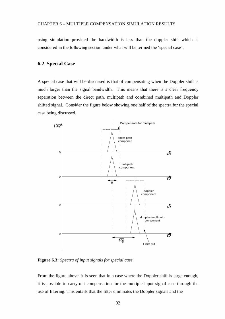
92


using simulation provided the bandwidth is less than the doppler shift which is

considered in the following section under what will be termed the ‘special case’.

6.2 Special Case

A special case that will be discussed is that of compensating when the Doppler shift is

much larger than the signal bandwidth. This means that there is a clear frequency

separation between the direct path, multipath and combined multipath and Doppler

shifted signal. Consider the figure below showing one half of the spectra for the special

case being discussed.

0

0

0

0

direct pathcomponet

multipathcomponent

dopplercomponent

doppler+multipathcomponent

Compensate for multipath

Filter out

Bω

ω

ω

ω

( )f ω

dω

Figure 6.3: Spectra of input signals for special case.

From the figure above, it is seen that in a case where the Doppler shift is large enough,

it is possible to carry out compensation for the multiple input signal case through the

use of filtering. This entails that the filter eliminates the Doppler signals and the

93


combined multipath and Doppler shifted signals leaving the multipath and direct path

signal from which the direct path signal can be retrieved because the simulation now

reduces to a multipath compensation case which was handled already under multipath

compensation. The main condition applied to the case above is that the signal band

width ought to be less than the Doppler shift (i.e ωd > B). The filter leaves us with the

direct and multipath signal and therefore, the required direct path signal can eventually

be extracted using multipath compensation. The same special case scenario would

apply when the Doppler shift is much lower than the bandwidth of the signal.

Therefore, it suffices to say that philosophical ways of carrying out compensation can

be deduced but with specific conditions applied in each case.

6.3 Simulation Results

Figure 6.4 below shows the combined multipath and Doppler signal with its spectrum.

This signal is a time and Doppler shifted version of the direct path signal. The signal

was delayed in time first and then Doppler shifted. This signal brought about the

complexity of the compensation process and thus it was not possible to come up with a

combined transfer function from which Xd would be extracted from the received signal.

The signal and its magnitude spectrum are shown in the figure below.

0 500 1000 1500 2000 2500 3000 3500 40000

50

100

150

200

250

300magnitude spectrum of multipath + doppler signal

frequency(Hz)

mag

nitu

de

(b)

0 100 200 300 400 500 600 700 800 900 1000

-1

-0.8

-0.6

-0.4

-0.2

0

0.2

0.4

0.6

0.8

1

multipath+doppler signal

samples

ampl

itude

(a)

Figure 6.4: (a) Multipath and Doppler shifted signal. (b) Magnitude spectrum of signal.

For the above results, the sampling frequency was 4000Hz and the carrier frequency of

1000Hz. The Doppler shift used was 50Hz (large merely for analysis purposes).

94


The magnitude spectrum of the signal shows that there exists a Doppler shift and

multipath component in the signal. One of the challenges at the compensation stage

was in getting the correct domain in which the compensation must take place. Under

multipath, the compensation took place in the frequency domain whilst for Doppler

shift, we compensated in the time domain. Now this case presents a situation where we

had both present and hence this in itself presented a major problem in trying to carry out

the compensation process. The received signal and its spectrum are shown in the

figure below. As was mentioned earlier, if the Doppler shift were much larger than the

bandwidth, a possibility for compensation would exist and this is considered under the

‘special case’ later in the chapter.

0 500 1000 1500 2000 2500 3000 3500 40000

50

100

150

200

250

300

350

400magnitude spectrum of received signal

frequency(Hz)

mag

nitu

de

(b)

0 100 200 300 400 500 600 700 800 900 1000

-3

-2

-1

0

1

2

3

received signal

samples

ampl

itude

(a)

Figure 6.5: (a) Received signal (b) Magnitude spectrum of received signal.

At this point, the limitation facing the compensation process comes in. From the

simulation results, it was seen that the Doppler components aliased with the multipath

components and hence a successful compensation was not possible. The mathematical

analysis stalemate faced does halt the compensation process at this stage. However, as

was discussed under the special case, the compensation is possible for the simulation

despite the barrier faced from the theoretical analysis and this is on condition that the

bandwidth-doppler shift ratio is small or less than 1.

95


6.4 Special Case:– Simulation results for Radio frequency

Figure 6.6(a) below shows the received signal having all the four input signals added

together and the resulting spectrum shown in (b). Here it is clear to see the separation

between the multipath, direct path, Doppler and multipath and Doppler spectral

components. The Doppler shift used was exaggerated to 500Hz which was large enough

for analytical purposes so as to clearly see the separation in the spectral components.

Therefore, it is intended to eliminate the Doppler and multipath components of the

spectrum and hence the need to filter out the unwanted part.

0 100 200 300 400 500 600 700 800 900 1000

-3

-2

-1

0

1

2

3

received signal

samples

ampl

itude

(a)

0 500 1000 1500 2000 2500 3000 3500 40000

50

100

150

200

250

300

350


frequency(Hz)

mag

nitu

de

(b)

Figure 6.6: (a) Received signal (b) Magnitude spectrum of received signal.

The figures on the next page show the filtered spectrum and the compensated spectrum

resulting from the compensation process. Figure 6.7(a) shows the filtered spectrum of

the received signal. It is seen that the Doppler content of the spectrum has been filtered

out together with the combined multipath and Doppler shifted signal components. This

leaves the multipath and direct path components from which the multipath component

was eliminated by the carrying out multipath compensation as was done in Chapter 4.

96


0 500 1000 1500 2000 2500 3000 3500 40000

50

100

150

200

250

300

350

400magnitude spectrum of received signal after filtering

frequency(Hz)

mag

nitu

de

(a)

0 500 1000 1500 2000 2500 3000 3500 40000

50

100

150

200

250

300magnitude spectrum of compensated signal

frequency(Hz)

mag

nitu

de

(b)

Figure 6.7: Spectral plots of :(a) Filtered received signal (b) Compensated signal.

The figures on the next page show the resulting compensated demodulated outputs xrcd1

and xrcd2 and the difference plot which is a plot of the numerical difference between the

compensated demodulated output and the direct-path demodulated outputs xd1 and xd2.

97


0 100 200 300 400 500 600 700 800 900 1000-1

-0.8

-0.6

-0.4

-0.2

0

0.2

0.4

0.6

0.8


samples

ampl

itude

0 100 200 300 400 500 600 700 800 900 1000-1

-0.8

-0.6

-0.4

-0.2

0

0.2

0.4

0.6

0.8

1Compensated demodulated output

samples

ampl

itude

xrcd1

xrcd2

(b)

0 100 200 300 400 500 600 700 800 900 1000-1

-0.8

-0.6

-0.4

-0.2

0

0.2

0.4

0.6

0.8

1Direct path demodulated output

samples

ampl

itude

xd1

xd2

(c)

(a)

0 100 200 300 400 500 600 700 800 900 1000-0.05

-0.04

-0.03

-0.02

-0.01

0

0.01

0.02

0.03

0.04

0.05compensated demodulated output - direct path demodulated output

xd1-xrcd1

xd2-xrcd2

(d)

Figure 6.8: (a) Compensated received signal (b) Compensated demodulated outputs

signal. (c) Direct-path demodulated outputs (d) Difference plot.

The error/difference plot show shows a small error and is evident of a successful

compensation process carried out under the special case. It therefore suffices to

conclude that it is possible to compensate simultaneously for multipath and Doppler

shift provided the Doppler shift is greater than the signal bandwidth. The analysis now

moves to quadrature baseband so as to see whether the special case is applicable at QBB

too.

6.5 Special Case – Simulation results for Quadrature baseband

The figures on the next page show the plots resulting from the simulation carried out at

QBB.

98


-4 -3 -2 -1 0 1 2 3 4-4

-3

-2

-1

0

1

2

3

4received QAM modulated down-mixed signal

real part

imag

inar

y pa

rt

(a)

0 500 1000 1500 2000 2500 3000 3500 40000

50

100

150

200

250

300

350

400magnitude spectrum of down-mixed signal

frequency(Hz)

mag

nitu

de

(b)

0 100 200 300 400 500 6000

50

100

150

200

250

300

350


samples

mag

nitu

de

(d)

0 100 200 300 400 500 6000

100

200

300

400

500


samples

mag

nitu

de

(f)

-4 -3 -2 -1 0 1 2 3 4-4

-3

-2

-1

0

1

2

3

4received QAM QBB signal

real part

imag

inar

y pa

rt

(c)

-2.5 -2 -1.5 -1 -0.5 0 0.5 1 1.5 2 2.5-2.5

-2

-1.5

-1

-0.5

0

0.5

1

1.5

2

2.5compensated QBB signal

real part

imag

inar

y pa

rt

(e)

Figure 6.9: Simulation results. (a) Down-mixed received signal (b) Down-mixed signal

spectrum (c) QBB received signal.(d) QBB received signal spectrum (e) Compensated

QBB signal (f) Compensated downsampled QBB signal spectrum. The sub-sampling

factor used was 2.

99


The plots in the figures on the previous page show the simulation results for the QBB

compensation analysis. As mentioned earlier, downsampling was carried out and hence

the sample reduction from 1024 to 512 due to the downsampling factor of ‘2’.

The spectral changes are also shown and it is seen that the uncompensated QBB

spectrum has the Doppler components filtered out and it was seen that the same filter

used in achieving QBB was used to filter out the Doppler components of the spectrum.

The signal now sits at QBB and compensation was carried out at this stage. The real

and imaginary parts were then taken to give the demodulated output signals y1 and y2

shown below.

0 50 100 150 200 250 300 350 400 450 500

-1

-0.8

-0.6

-0.4

-0.2

0

0.2

0.4

0.6

0.8

1

compensated received QBB demodulated signal

samples

ampl

itude

y1

y2

(a)

0 50 100 150 200 250 300 350 400 450 500-0.1

-0.08

-0.06

-0.04

-0.02

0

0.02

0.04

0.06

0.08


xd1-y1

xd2-y2

(b)

Figure 6.10: (a) Compensated demodulated output. (b) Difference plot.

The difference plot above where xd1 and xd2 are the direct-path demodulated outputs

shows that the compensation was successful with the error having a maximum value of

approximately 3%.

6.6 Benefits of Multiple compensation at QBB

The sample processing and simulation runtime results are now compared for the RF and

QBB QAM simulation for the multiple input signal case. As mentioned earlier, the

comparison starts from the received signal stage through the compensation and down to

the demodulation. The tables on the next page summarize the sample processing and

simulation runtime at RF and QBB.

100


Simulation Stages Radio Frequency Quadrature baseband

Mixing down + QBB +

Down sampling

____ N + NLog2N

2kN + kNLog2kN

Compensation process

NLog2N

N+ NLog2N

N

kN + 2kNLog2kN+2kN

kN + 2kNLog2kN

kN + 2kNLog2kN +

kN +2 kNLog2kN

Demodulation 2NLog2N+2N

2NLog2N

_____

Total sample processing 4N+ 6NLog2N N+8kN+NLog2N+

9kNLog2kN

Total sample processing

for N=1024 and k=1/2 67584 56832

Table 6.1: Sample processing at RF and QBB.


MIMO compensation Time in seconds Ratio Number of

Calculations Ratio

QAM 0.00122 0.00099 1.23 67584 56832 1.19

Table 6.2: Simulation runtime and sample processing ratio summary. The discrepancy

between the sample processing ratio and simulation runtime is 3.25% which is

reasonable enough given the variance in the computer processing time.

The results interms of the simulation runtime and number of calculations, we see a

significant reduction in the ratios for the multiple compensation case. From the Table

6.1 it can be seen that despite the downsampling process, the number of

calculation/operation taking place at QBB is a lot and as such the expected advantage

interms of reduced number of calculations and reduced simulation runtime is not as

large as in the previous analysis. The analogue QBB case too has a ratio output equal

to:

101

CHAPTER 6 – MIMO COMPENSATION: SIMULATION RESULTS

675841.48

45568rf

qbb

N

N= = (6.5)

It was seen that the analogue QBB case still proved slightly more advantageous than the

digital QBB case. However, we still saw a reduction in terms of the ratio for the

analogue case as compared to the values obtained in the previous analysis. The

simulation runtime should follow a similar trend.

6.7 Conclusion

The study carried out showed that compensating for multipath and Doppler shift

simultaneously a complicated and tedious task for cases where the Doppler shift is less

than the signal bandwidth. The compensation was however, possible for a smaller

bandwidth- doppler shift ratio and its is true to say that the smaller the ratio, the better

the compensation due to the easier filtering out of the Doppler components. This

presents a case where the simulation results had to be relied upon despite the stalled

mathematical analysis. The study considered QAM only because the same limitations

faced under QAM would be encountered under FM. It therefore, suffices to say that

compensating for multipath, Doppler shift simultaneously being reflective of a MIMO

system where we have multiple signals inputs and a single output is possible but under

certain conditions. An area of application is in multi-rate digital signal processing

techniques which improves the flexibility of software defined radio [23]. The benefits

for working at QBB here were seen to be less pronounced for this case as compared to

the previous analysis carried out but still, QBB does have the upper hand. Thus it is

seen that indeed the processing load at QBB was less and this equally translated to a

reduction in the processing time.

102

Chapter 7 Matched Filter Detection This part of the overall study ventures into the digital signal arena by analyzing a simple

chirp signal where a positive chirp represents a digital ‘1’ and its absence represents a

digital ‘0’. The analysis carried out involved carrying out matched filter detection of

the chirp signal at RF and QBB for different cases which include multipath, Doppler

shift and a combination of the two as was done in the previous study which involved

compensating for these effects. The study firstly assumes noiseless channels and

considers one case involving matched filter detection in a noisy channel. The core

purpose of the study remains investigating carrying various signal processing

techniques at QBB with the main advantage of working at QBB being the low operating

frequencies involved.

7.1 Matched Filter Detection

Before going down to the analysis results, it is necessary to get a brief background of

matched filter detection so as to understand the resulting outputs from the simulations

carried out. Matched filtering is a process known to be the optimum linear filter for

detecting a known signal in random noise [29]. The DSP responsible for the processing

of signals has a copy of the signal it should detect. It then time reverses the signal for

detection and cross-correlates it with the received signal [38]. A detailed derivation of

the matched detector is given in Appendix B.

The study looked at matched filter detection for noiseless transmissions before

looking at the real life situation where noise is a factor that affects the detection process.

The study looked at the direct path signal with no multipath or Doppler shift effects and

then subsequent simulations were carried out where multipath and Doppler shift were

introduced. As mentioned earlier the signal used in the simulations was a chirp signal

whose generation is discussed in the next section.

103

CHAPTER 7 – MATCHED FILTER DETECTION: SIMULATION RESULTS

7.2 Matched filter detection:- noiseless channels

The analysis was firstly carried out at RF and this involved analyzing the direct path,

multipath, Doppler shift and the combined multipath and Doppler shift cases. The

results will then be compared with there corresponding results achieved at QBB so as to

come up with a conclusion about investigating the results obtained at QBB coupled with

the already mentioned benefits of working at QBB.

7.2.1 Theoretical analysis:- RF

Consider the block diagram below which illustrates the analysis process carried out at

RF.

Matched filterdetector

h

xd y

Figure 7.1: RF chirp signal matched filter detection

The input chirp signal is fed into a matched filter whose output is a convolution between

the received signal and its time reversed version. Let the chirp input be xd . Matlab

uses an inbuilt command to execute the time reversal of the chirp input ‘xd’.

( )dh flipr x= (7.1)

The matched filter then convolves the chirp input ‘x’ with h given as

( , )dy conv x h= (7.2)

The matched filter output has its peak value at t=T. The theoretical analysis for the

QBB simulations is given in the next section and the simulation results which follow in

subsequent sections of the chapter will compare the results obtained at RF and QBB for

the multipath, Doppler shift and the combined multipath and Doppler shift cases.

104


7.2.2 Theoretical analysis QBB

The sole purpose of the study is to investigate the possibility of carrying out certain

signal processing techniques at quadrature baseband and hence, it is required to outline

the theory used to carryout the simulations at QBB.

Consider the figure below

Matched filter'h'detector

atQBB

X

cj te ω−

LPFdx dqbbx y

downsampling takes placehere

Figure 7.2: QBB chirp signal matched filter detection.

From the figure above, it is seen that the chirp is mixed down and lowpass filtered to

quadrature baseband before being fed into the matched filter which has a time-reversed

copy of the QBB input chirp. The output does have its peak at t=T as in the previous

RF analysis. The simulation results will give a more detailed comparison of the

graphical results obtained from the RF and QBB simulations.

| .* |cj tqbb LPFx x e ω−∴ = (7.3)

The matched filter output should show a perfect match occurs when the QBB chirp

input and its time-reversed copy make a complete overlap at t=T resulting in the large

spike at that point. A piece of Matlab code used to implement the matched filter

detection at QBB is given below:

h=conj(fliplr((xqbb))); % matched filter at QBB y=real(conv(xqbb,h)); % takes place at QBB

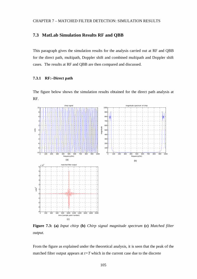
105


7.3 MatLab Simulation Results RF and QBB

This paragraph gives the simulation results for the analysis carried out at RF and QBB

for the direct path, multipath, Doppler shift and combined multipath and Doppler shift

cases. The results at RF and QBB are then compared and discussed.

7.3.1 RF:–Direct path

The figure below shows the simulation results obtained for the direct path analysis at

RF.

0 100 200 300 400 500 600 700 800 900 10000

100

200

300

400

500

600

700

800

900

1000magnitude spectrum of chirp

mag

nitu

de

frequency(Hz)

(b)

0 200 400 600 800 1000 1200 1400 1600 1800 2000-4

-3

-2

-1

0

1

2

3

4

5

6x 10

4 matched filter output

time (sample point number)

volts

2

0 100 200 300 400 500 600 700 800 900 1000-10

-8

-6

-4

-2

0

2

4

6

8

10chirp signal

frequency(Hz)

volts

(a)

(c)

Figure 7.3: (a) Input chirp (b) Chirp signal magnitude spectrum (c) Matched filter

output.

From the figure as explained under the theoretical analysis, it is seen that the peak of the

matched filter output appears at t=T which in the current case due to the discrete

106


domain being used, the point T corresponds to the sample point number n= 1024. The

matched filter output has a peak value of 5.12e4 at this point and this value was verified

mathematically. Let y(n) represent the matched filter output in the discrete domain. As

mentioned earlier the convolution is a point-wise multiplication and integration which

in the discrete domain is represented by the following operation.

1

( ) ( ) ( )N

n

y n x n h n=

=∑ (7.4)

Now for the current simulation, the input chirp x was sinusoidal having a peak value of

10 and the sampling frequency fs being 1000Hz. Replacing the expressions for x(n) and

h(n) with the discrete domain versions of x(t) and h(t) and ignoring other parameters of

the chirp expect for the amplitude and signal form( i.e. sine or cosine)

We have;

1024

1

( ) ( ) ( )N

n

y n x n h n=

== ∑ (7.5)

or

1024

1

( ) (10sin[...])(10sin[...]) *N

n

y n=

== ∑ (7.6)

Note that the ‘*’ denotes the conjugate of the time-reversed version of the chirp. It is

seen that a product of the two inputs of Equation 7.7 summed from n= 1 to N results in

a trigonometric expression given below which upon applying a trigonometric identity

reduces to the Equation 7.8 below.

1024

2

1

( ) 100sin [....]n

y n=

=∑ (7.7)

or

1024

1

1 1( ) 100( cos 2[....])

2 2n

y n=

= −∑ (7.8)

The absolute value of the matched filter output thus reduces to:

107


41| ( ) | (1024 100) 5.12 10

2y n = × = × (7.9)

Therefore, the output of the matched filter was correct as has been verified numerically.

7.3.2 QBB:- Direct path

The analysis then moves down to quadrature baseband where the matched filter

detection is now being implemented at QBB. The figures shown below are the

simulation results obtained from the QBB simulation. The parameters of the input chirp

are the same as those used for the RF simulation.

0 100 200 300 400 500 600 700 800 900 10000

100

200

300

400

500

600

700

800

900

1000magnitude spectrum of down-mixed chirp

mag

nitu

de

frequency(Hz)

(a)

-15 -10 -5 0 5 10 15-15

-10

-5

0

5

10

15QBB chirp

imag

inar

y ax

is

real axis

(c)

0 50 100 150 200 2500

50

100

150

200

250

300

350

400

450

500magnitude spectrum of QBB chirp

mag

nitu

de

samples

(b)

0 50 100 150 200 250 300 350 400 450 500-2

-1

0

1

2

3

4

5

6x 10



volts

2

(d)

Figure 7.4: Simulation plots.(a) Magnitude spectrum after down-mixing (b) After

lowpass filtering and downsampling (c) QBB chirp (d) Matched filter output.

108


The figures on the previous page show the conversion of the chirp to quadrature

baseband and the final matched filter detected output shown in Figure 7.4(d). It is seen

that downsampling is done at QBB and this reduced the samples by a factor of 4. Thus

the point-wise multiplication done by the matched filter takes place on fewer samples

and hence the sample processing is expected to be less which should translate to less

processing time. The maximum value of the matched filter shifts to the 256th sample

point after the downsampling. This presents an advantage of carrying out matched filter

detection at QBB compared to doing so at RF.

7.4 RF:- Multipath

The study then looked at a scenario where it was now assumed that the transmission is

subjected to multipath effects. This part of the study is relevant in that when applied or

related to digital transmissions, we are looking at a case where we have a bit stream

transmitted followed by its delayed version. Now in this case, we are considering

matched filter detection and seeing how the matched filter output can influence the

making of a correct decision during the detection process. Similarly, it is assumed for

analytical purposes that we have a noiseless transmission. The parameters of the input

chirp used in this simulation remains the same as used for the RF direct path case and

this is for purposes of comparing the changes that are brought about by the fact that we

now taking into consideration the multipath signal too in the matched filter detection.

The figure below shows the block diagram for the multipath analysis simulation. The

echo factor ‘k’ in the multipath signal is assumed to be equal to 1 for simplicity’s sake

in the analysis process.

Matched filter detector

MF detector output

direct path + multipathsignal

∑Chirp

Chirpdelayed chirp

k t∆

Figure 7.5: Multipath RF simulation flow.

109


The generation of the delayed version of the original chirp is done in the same way as

the delayed signals were generated under the previous study on multipath

compensation. The figures below show the results obtained from the multipath analysis

simulation.

0 100 200 300 400 500 600 700 800 900 1000-20

-15

-10

-5

0

5

10

15

20received multipath chirp signal

freq(Hz)

volts

0 100 200 300 400 500 600 700 800 900 10000

200

400

600

800

1000

1200

1400

1600

1800magnitude spectrum of received multipath chirp

mag

nitu

de

frequency(Hz)

0 200 400 600 800 1000 1200 1400 1600 1800 2000-1.5

-1

-0.5

0

0.5

1

1.5

2x 10



volts

2

(a) (b)

(c)

Figure 7.6: (a) Received multipath chirp (b) Magnitude spectrum (c) Matched filter

output.

From Figure 7.6 (a) it is seen that the amplitude of the received signal has increased and

the signal amplitude decreases as the frequency approaches 1000Hz. This is due to the

phase changes whose effects at higher frequencies result in the decreased amplitude due

to the out-of-phase summations of the direct path and time delayed signals taking place

as the frequency increases. A look at the magnitude spectrum also shows a considerable

increase brought about by the multipath and hence it is expected that the matched filter

output will follow suit and indeed it does so as shown in Figure 7.6(c). This result

entails that there is increased signal strength at the output of the matched filter and this

110


energy can be made use of in the detection process.

7.5 QBB:- multipath

The block diagram below illustrates the simulation flow for the analysis carried out at

quadrature baseband. The input parameters remain the same as used for the RF

simulation.

Matched filter detectorat QBB

MF detector output

direct path + multipathsignal

∑

k t∆

Chirp

Chirp delayed chirp

X LPF

cj teω−

QBB signal


Figure 7.7: QBB Matlab simulation flow.

The figure above shows that the received signal is down-mixed and then lowpass

filtered down to quadrature baseband before being fed into the matched filter which sits

at QBB enabling the detection process to take place at QBB. The simulations results

resulting from this simulation are shown in the Figure 7.8 (a), (b), (c) and (d) on the

next page. The downsampling reduced the sample point number by a factor of 4. The

peak value of the output remains the same as for the RF case entailing that it is equally

possible to carry out the matched filter detection at QBB with similar results being

obtained. The advantages of this in terms of sample processing and simulation runtime

have been discussed earlier.

The spectral changes are notable as was seen under the RF analysis where it was

observed that there was an increase in the magnitude of the magnitude spectrum which

eventually resulted in increased signal strength at the output of the matched filter and

the advantages brought about by this in terms of the detection process in digitals

transmissions has been explained. Therefore, it was seen from the results that we can

equally carry out matched filter detection at QBB frequencies just as it is done at RF.

111


0 100 200 300 400 500 600 700 800 900 10000

200

400

600

800

1000

1200

1400

1600

1800magnitude spectrum of down-mixed chirp

mag

nitu

de

frequency(Hz)0 50 100 150 200 250

0

100

200

300

400

500

600

700

800

900magnitude spectrum of QBB chirp

mag

nitu

de

samples)

0 50 100 150 200 250 300 350 400 450 500-1.5

-1

-0.5

0

0.5

1

1.5

2x 10



volts

2

(d)

(a) (b)

(c)

-25 -20 -15 -10 -5 0 5 10 15 20 25-25

-20

-15

-10

-5

0

5

10

15

20

25QBB chirp

imag

inar

y ax

is

real axis

Figure 7.8: Simulation plots. (a) Received signal magnitude spectrum (b) After down-

mixing and downsampling (c) After lowpass filtering (d) Matched filter output.

From Figure 7.8(d) it is seen that due to the downsampling, the maximum output of the

matched filter now occurs at the 256th sample point. The peak value of the matched

filter output for the QBB case is the same as that obtained at RF despite the sample

reduction brought about by the downsampling. Overall, it can be concluded for both the

RF and QBB cases that the multipath effects actually enhance the signal detection of the

matched filter by increasing the signal strength and hence resulting in increased signal

strength for the matched filter. Going by the aim of the study, it is seen that indeed we

were able to carry out the matched filter detection at lower QBB frequencies and at the

same time at lower sampling rates brought about by the further sub-sampling that was

carried out.

112


7.6 RF:-Doppler shift

The simulation moved on to look at the Doppler shift scenario so as to analyze the

changes that take place in the matched filter output due to the doppler shifting effects.

The block diagram below illustrates the simulation flow.

Matched filter detectorMF detector outputf∆Chirp


Figure 7.9: RF simulation flow.

The generation of the Doppler shifted version of the chirp signal is done in the same

way as was done for the Doppler shift compensation analysis. The figures below show

the simulation results.

0 100 200 300 400 500 600 700 800 900 1000-15

-10

-5

0

5

10

15received Doppler shifted chirp signal

freq(Hz)

volts

0 100 200 300 400 500 600 700 800 900 10000

100

200

300

400

500

600

700

800

900

1000magnitude spectrum of doppler shifted chirp

mag

nitu

de

frequency(Hz)

(b)

0 200 400 600 800 1000 1200 1400 1600 1800 2000-6

-4

-2

0

2

4

6x 10



volts

2

(a)

(c)

Figure 7.10: Simulation plots (a) Doppler shifted chirp (b) Magnitude spectrum of MF

input signal (c) MF output.

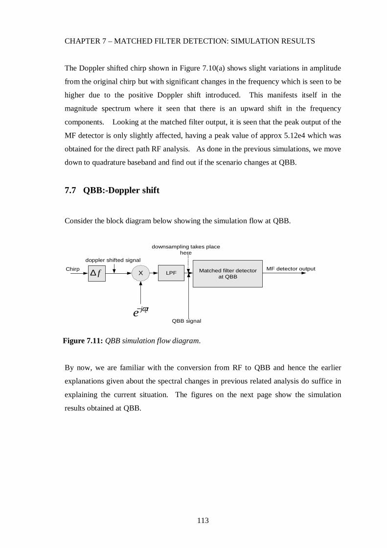
113


The Doppler shifted chirp shown in Figure 7.10(a) shows slight variations in amplitude

from the original chirp but with significant changes in the frequency which is seen to be

higher due to the positive Doppler shift introduced. This manifests itself in the

magnitude spectrum where it seen that there is an upward shift in the frequency

components. Looking at the matched filter output, it is seen that the peak output of the

MF detector is only slightly affected, having a peak value of approx 5.12e4 which was

obtained for the direct path RF analysis. As done in the previous simulations, we move

down to quadrature baseband and find out if the scenario changes at QBB.

7.7 QBB:-Doppler shift

Consider the block diagram below showing the simulation flow at QBB.


MF detector outputX LPF

cj teω−

QBB signal

f∆Chirp



Figure 7.11: QBB simulation flow diagram.

By now, we are familiar with the conversion from RF to QBB and hence the earlier

explanations given about the spectral changes in previous related analysis do suffice in

explaining the current situation. The figures on the next page show the simulation

results obtained at QBB.

114


0 100 200 300 400 500 600 700 800 900 10000

100

200

300

400

500

600

700

800

900

1000down-mixed doppler shifted signal spectrum before filtering

freq(Hz)

volts

(a)

0 50 100 150 200 2500

50

100

150

200

250

300

350

400

450

500QBB doppler shifted signal spectrum

samples

volts

(b)

0 50 100 150 200 250 300 350 400 450 500-4

-3

-2

-1

0

1

2

3

4

5

6x 10



volts

2

(d)

-15 -10 -5 0 5 10 15-15

-10

-5

0

5

10

15QBB doppler shifted chirp signal

real axis

imag

inar

y ax

is

(c)

Figure 7.12: Simulation plots (a) Magnitude spectrum of down-mixed Doppler shifted

chirp (b) Magnitude spectrum of QBB chirp (c) QBB chirp (d) QBB Doppler shifted

signal.

From Figure 7.12(d) it is seen that the Doppler shift effect on the maximum value of the

matched output is minimal. Therefore, it has been shown here that the matched filter

detection can take place at QBB and with the further sub-sampling that takes place, it is

seen that the processing load reduced which should further translated to a reduction in

the simulation processing time. This will be shown in a later part of the chapter.

115


7.8 Multiple signal reception:- Radio frequency

The block diagram below summarises the simulation flow for the case at hand.

Matched filter detector(matched to received

signal)

matched filter output

multipath + doppler shiftedsignal

multipath signal

k t∆ f∆

1

Chirp


direct pathsignal

k t∆

f∆

∑

Received signal

Figure 7.13: RF simulation flow:- It should be noted that the matched filter is matched

to the complex received signal comprising the four input signals summed together.

The analysis now considers a case of multiple signal reception and investigates the

changes observed at the matched filter output due to the multiple signal input to the

matched filter. The same mode of generation of the multipath and Doppler shifted

signal used for under the compensation analysis is used in the current analysis.

116


0 100 200 300 400 500 600 700 800 900 10000

200

400

600

800

1000

1200

1400

1600


mag

nitu

de

frequency(Hz)

(a)

0 100 200 300 400 500 600 700 800 900 1000-40

-30

-20

-10

0

10

20

30

40received chirp signal

freq(Hz)

volts

0 200 400 600 800 1000 1200 1400 1600 1800 2000-3

-2

-1

0

1

2

3

4x 10



volts

2

(b)

(c)

Figure 7.14: Simulation results.(a) Received signal magnitude spectrum (b) Received

Multipath and Doppler shifted signal .(c) Matched filter output.

The magnitude spectrum in Figure 7.14(a) shows the multipath and Doppler shifted

components of the received signal. A glance at the spectrum shows that it is a

combination of the two spectrums for the separate analysis carried out for multipath and

the Doppler shift. The matched filter output is thus expected to have a larger output

peak signal strength due to the presence of more signals whose energies are utilised

which when added up gave a much stronger signal and this is clearly seen in Figure

7.14(c).

117


7.9 Multiple signal reception:- Quadrature baseband

The figure below summarizes the simulation flow for the QBB analysis.


(matched to receivedQBB signal)

matched filter output

multipath + doppler shiftedsignal

multipath signal

k t∆ f∆

1

Chirp


direct pathsignal

k t∆

f∆

∑ X LPF

Received QBB signal

cj te ω−

downsampling is donehere

Received signal

Figure 7.15: QBB simulation flow:- the figure above clearly shows the 4 input signal

paths up to the point of summation. The mixing down follows and lowpass filter moving

the process down to QBB and after downsampling the matched filter detection takes

place.

As seen above, the procedure remains the same as in the previous analysis with the

same signal parameters being used for the sake of carrying out an effective comparison.

The figure on the next page show the simulation results for the QBB analysis.

118


0 100 200 300 400 500 600 700 800 900 10000

200

400

600

800

1000

1200

1400

1600

1800down-mixed received signal spectrum before filtering

freq(Hz)

mag

nitu

de

(a)

-60 -40 -20 0 20 40 60-60

-40

-20

0

20

40

60QBB received chirp

real axis

imag

inar

y pa

rt

0 50 100 150 200 250 300 350 400 450 5000

200

400

600

800

1000

1200

1400

1600

1800QBB received signal spectrum

samples

mag

nitu

de

0 100 200 300 400 500 600 700 800 900 1000-4

-2

0

2

4

6

8

10x 10



volts

2

(b)

(c) (d)

Figure 7.16: Simulation results (a) Magnitude spectrum of down-mixed chirp (b) QBB

magnitude spectrum (c) MF detector output.

The magnitude spectrum in Figure 7.16(a) shows the direct-path, multipath and Doppler

shift components of the received signal. The downsampling factor in this case was 2.

A further increase in the factor resulted in aliasing and hence the need to limit the factor

to ‘2’. The matched filter detection which takes place at QBB gives the output shown in

Figure 7.16 (d). From the resulting output, it is seen that output signal strength is more

than that for the individual direct-path, multipath and Doppler shift cases and thus hence

the detection process is more enhanced for the multiple input signal case. Indeed, it has

been shown that the matched filter detection could take place at QBB at much lower

sampling rates. The comparison in terms of the amount of processing for the RF and

QBB cases is given in a later part of the chapter.

119


7.10 Matched filter detection:-Noisy channel

One common problem in signal processing is that of detecting the presence of a known

signal against a background of noise. The main application for matched filtering

techniques is in the detection of known deterministic signals in a background of random

noise disturbances [4].

7.10.1 Matched Filter Detection- RF

The flow diagram below illustrates the analysis used for the matched filter detection in a

noisy channel. It should be noted that the chirp generation remains the same as for the

noiseless cases.

Chirp signal input

Add WhiteGaussian Noise

Matched FilterDetection

Thresholddetector/decision

process

Store decision/result

Simulation & Theoreticalprobability of error

plotting

Repeat Loop forn times

increasenoise level

in dBs

Figure 7.17: RF simulation flow diagram.

120


The Figure on the previous page represents a model used to simulate a matched filter

detector in a noisy channel. The Gaussian noise [14, 37] is added to the input chirp and

fed to the matched filter detector which has a copy of the original transmitted chirp.

The Gaussian noise generated has a normal distribution with a mean = 0 and a standard

deviation = 1. This is made possible by use of the MatLab command ‘randn’.

This part of the study considered a noisy channel and it was required to investigate the

matched filter output for detection in a Gaussian distributed noise channel at RF and

QBB. Appendix B gives more detail about matched filter detection in a noisy channel.

The study basically aims to investigate the possibility of carrying out matched filter

detection in a noisy channel at QBB and therefore, going into details of the matched

filter detection does not serve the main purpose of the study. The results from the

simulations carried out at RF and QBB are discussed later in the chapter. In this case,

the signal-to-noise ratio factor comes into play and therefore, the simulation needs to be

run several times in order to eventually come up with a probability of error plot. In this

particular analysis, a positive chirp was generated and transmitted in a noisy channel

before the matched filter receives the signal and convolves it with a copy of the time

reversed original signal. A threshold detector at the output of the matched filter carries

out the decision making process. If the MF output is greater than zero, the decision is

‘1’ and if the output is less than zero, the decision is ‘0’. The mathematical derivation

for the theoretical probability of error is given in Appendix A. The loop was run 1e6

times in order to achieve the results shown in the graphical plots. It should therefore be

noted that the larger the number of runs, the better the matching between the simulation

probability of error and the theoretical one. Appendix A also gives the values for the

simulation and theoretical probability of error obtained for the direct path case. The

noise level in the signal is increased and the loop runs through again and hence the

matched filter detection process equally takes place repeatedly. MatLab however only

shows the last value of the loop. An extract of part of the MatLab code executing the

RF simulation flow illustrated in the previous figure is given on the next page.

121


----------------------------------------------------------------------------------------------------------

nch=1e7/sqrt(10.^(dB/10)); %noise power defined with respect to varying dBs %--------------------------------------------------------------------- for i=1:1:n noise=randn(1,N)*nch; xr=x + noise; % received signal y=conv(xr,h); p=y(1024); if p>0, decision(i)=1; % chirp is detected else decision(i)=0; % chirp is not detected end; end; Proberr(dB)=1-(nnz(decision)/n); % calculates the simulated probability of error. M=5.12e4; Sigma=nch*sqrt(5.12e4) Theor=0.5*qrfc(m./(sqrt(2)*sigma)) % calculates the theoretical probability of error. end; -----------------------------------------------------------

The decision is made at the point where y=1024 because the sampling frequency used is

1024 and hence N=1024. The complete MatLab script is can be accessed from the M-

Files on the CD in Appendix C. The code therefore shows that for a noise power that

has its dB level changing and the simulation runs through from n=1 to n=1e6 and makes

a decision n times. This enables and error probability for each dB level to be calculated

resulting in a probability of error plot. The in built MatLab function ‘nnz’ gives the

number of non-zero values in a vector and hence is used to give the number of ones

from the decision vector which when subtracted from one gives the actual number of

zeros (errors). The next section of the chapter gives the simulation results.

7.10.2 Simulation results:- Radio Frequency.

The figures on the next page illustrate the results obtained form the simulation at RF.

The first figure shows the received signal for the last value of n which in our case was

1e6 implying that the loop was run 1e6 times. The matched filter convolves the original

signal with the received noisy signal and decision is eventually made based on the

matched filter output at N=1024. The matched filter output shown in Figure 7.18 (b) on

the next page represents the last value of the matched filter and Figure 7.18(c)

represents the probability of error plots for both the theoretical and simulation analysis.

122


(a) (b)

(c)

0 200 400 600 800 1000 1200-300

-200

-100

0

100

200

300

400received signal

samples

ampl

itude

0 500 1000 1500 2000 2500-6

-4

-2

0

2

4

6

8x 10



volts

2

Figure 7.18: Simulation results. (a) Received noisy signal:- the last plot of the received

signal shows the signal engulfed in noise. (b) Final plot of matched filter output:-shows

that the last value of the matched filter output at t=T is less than the expected value and

this due to noise which corresponds to the last plot of the received signal which has a

high level of noise. (c) Probability of error plots: the plots show that the simulation

probability of error does match with the calculated theoretical value.

The simulation moves down to quadrature baseband where received noisy signal now

sits at QBB and hence the matched filter detection is expected to take place at QBB too.

123


7.10.3 Matched Filter Detection- QBB

The simulation flow diagram given below summarizes the QBB analysis.

Chirp signal input

Add WhiteGaussian Noise

Matched FilterDetection at QBB

Thresholddetector/decision

process

Store decision/result

Simulation & Theoreticalprobability of error

plotting

Repeat Loop forn times

Down-mixing +lowpassfiltering

increasenoise level in

dBs

Downsamplingtakes place here

Figure 7.19: QBB simulation flow diagram.

The QBB simulation follows a similar looping process to the RF simulation except that

after the addition of the Gaussian noise, the signal undergoes conversion to quadrature

baseband facilitating for the matched filter detection process to take place at QBB. This

is the sole purpose of the study and hence the simulation results should verify the

possibility of working at quadrature baseband.

124


7.10.4 Simulation results:- Quadrature baseband

(a)

(c)

0 50 100 150 200 250 300 350 400 450 500-2

-1.5

-1

-0.5

0

0.5

1

1.5

2x 10


time (sample point number)vo

lts2

(b)

-150 -100 -50 0 50 100 150-150

-100

-50

0

50

100

150QBB received chirp

imag

inar

y ax

is

real axis

Figure 7.20: (a) QBB received chirp:-it is seen here that the signal is complex having a

real and imaginary part (b) Matched filter output:- the last value of the matched filter

shows that its maximum value at the 256th sample point is above zero which amounts to

a decision ‘1’. However, the intermediate values are present within the simulation. (c)

Probability of error plot:-the plots show that the simulated probability of error does

correspond with the theoretical probability of error entailing the correct operation of

the simulation. An increase in the number of runs would make the match much more

perfect.

125


The two curves in Figure 7.20(c) on the previous page show the probability of error

plots for the simulation and the theoretical probability calculated. It can be concluded

that the Matched filter detection at QBB was successful and that further adjustments in

the parameters used can result in better results. The sole purpose of this part of the

study has thus been achieved which is to carryout matched filter detection at QBB

accompanied with the excepted core benefit of working with at a lower sampling

frequency. Having considered the fact that working at QBB is of great benefit in terms

of sampling frequency and ultimately bandwidth requirements, the next section of the

chapter will consider the case of matched filter detection for multiple reception at QBB

whose results will be compared to the RF results through a comparison in terms of

probability of error ratios, simulation processing time and sample processing will be

made between the RF and QBB multiple signal reception simulations. Having thus far

seen the benefits of operating at QBB interms of sample processing reduction, the study

concludes by looking at the multiple signal reception case for matched filter detection at

RF and QBB.

7.11 Matched filter detection:- Multiple input signal at RF and QBB

The analysis finally looked at the reception of multiple signals. In this case the received

signal consists of the direct path chirp, a delayed version or multipath chirp and a

Doppler shifted version of the chirp. Noise is then added and then the signal is received

by the matched filter where detection takes place. In the QBB case, the signal gets

mixed down to quadrature baseband where the matched filter detection takes place. The

matched filter is matched to (a) direct path signal, (b) the direct path and multipath and

(c) a combination of the three signals, and the output is observed and three probability

of error plots are generated for each of the matched filters in both the RF and QBB

cases and then compared to the calculated theoretical probability of error plot.

Therefore, the generation of the input signals remains as given in an earlier part of the

chapter. The figures on the next page summarize the theoretical analysis for the radio

frequency and quadrature baseband simulations for the matched filter detection multiple

signal reception case. The focus is now on QBB having seen its benefits interms of

reduced sample processing.

126


In the figures that follow, xd represents the direct-path signal, xmp represents the

multipath signal and xdp represents the Doppler shifted signal.

+ + Matched filterat RF

(matched to xd)

Matched filterat RF

(matched toxd+xmp)

Matched filterat RF

(matched toxd+xmp+xdp)

Decision 1

Decision 2

Decision 3

xd

Gaussian noise(normally distributed)

k t∆

f∆

1eP

2eP

3eP

xdp

xmp xrxrn y1

y2

y3

received signal

Figure 7.21: Multiple signal input to matched filter detection at RF:- the 3 matched

filters result in 3 different outputs with different strengths.

The figure below summarises the theoretical analysis at QBB. The three match filters

are at QBB and matched to the different components of the multiple input signal.

+ + X LPF Matched filterat QBB

(matched to xd)

Matched filterat QBB

(matched toxd+xmp)

Matched filterat QBB

(matched toxd+xmp+xdp)

Decision 1

Decision 2

Decision 3

xd

Gaussian noise(normally distributed)

k t∆

f∆

cj te ω−

1eP

2eP

3eP

QBB signal (xrnqbb)

xdp

xmp xr xrn xrndm y1

y2

y3

downsamplingtakes place here

Figure 7.22: Theoretical flow QBB:-the expected signals at each point are shown in

this figure:- the decision is part of the simulation and details can be seen from the

simulation code.

127


The figure below shows the simulation flow for the matched filter detection analysis at

QBB. The RF flow diagram is similar to the QBB one but with the down-mixing, LPF

and downsampling stages omitted. The simulation loops are also shown. Each block

represents a piece of the overall MatLab code.

Add Normallydistributed Gaussian

noise

Increase noiselevel in dBs

Downmixing and LPF(QBB signal)

MF1(Matched filter at QBB

matched to xd)

MF2(Matched filter at QBB

matched to xd+xmp)

MF3(Matched filter at QBBmatched to xd+xmp+xdp )

Decision process basedon matched filter output



Store decision/result Store decision/result Store decision/result

Repeat loop for ncycles

Generate xd, xmp and xdp and sumthem up

Simulation probability oferror generation and

plotting


plotting


plotting

Downsampling donehere

Figure 7.23: Simulation flow: summarizes the flow of the simulation and each block

represent a part of the main MatLab code used for the whole process. The first loop

shows that the noise is increased in line with the dB range given so as to eventually

come up with the probability of error over that dB range for a given number of runs.

128


7.11.1 Simulation results:- Matched filter detection at RF

The simulation results are given in the figures below. It should be noted that MatLab

only shows the last values of a simulation loop and therefore intermediate values do

exist. The resulting probability of error plots are shown on the next page.

0 200 400 600 800 1000 1200 1400 1600 1800 2000-8

-6

-4

-2

0

2

4

6

8

x 104 matched filter output (matched to xd)


volts

2

(b)

0 200 400 600 800 1000 1200 1400 1600 1800 2000

-6

-4

-2

0

2

4

6

8x 10

4 matched filter output (matched to xd + xmp)


volts

2

0 200 400 600 800 1000 1200 1400 1600 1800 2000

-1.5

-1

-0.5

0

0.5

1

1.5

2

x 105 matched filter output (matched to xd + xmp + xdp)


volts

2

(d)

0 100 200 300 400 500 600 700 800 900 1000-30

-20

-10

0

10

20

30received chirp signal

freq(Hz)

volts

(a)

(c)

Figure 7.24: (a) Received summed input signal:- the input to the chirp consists of the

three signals which are summed up together. (b) Matched filter output when matched to

xd. (c) Matched filter output when matched to xd + xmp (d) Matched filter output when

matched to xd + xmp + xdp :- the last value of the matched filter output which was

matched to the direct path signal xd. It is seen that the maximum value of the matched

filter output is the largest for this output due to more signal strength brought about by

the three input signals.

129


The figure below shows the probability of error plots for the different matched filter

outputs. It is seen from the plots that the results further verify the matched filter

outputs as it can be seen that the probability of error gets smaller as the we move from

the 1st matched filter output to the 2nd and 3rd matched filter outputs due to increased

signal strength caused by the matched filter locking on to all the available energy in the

received signal.

Figure 7.25: Probability of error plots for multiple input signal matched filter detection

at RF.

7.11.2 Simulation results:- Matched filter detection at QBB

The figures on the next page show the matched filter outputs for the MIMO case at

QBB. The parameters used for the RF simulation are the same ones used in the QBB

simulation. For the QBB case, the downsampling comes into play and it thus

contributes to the reduced sample processing and hence less simulation runtime. In this

case, the downsampling factor used was equal to 4. Thus the decision point was made

at the 256th sample point of the matched filter output.

130


-300 -200 -100 0 100 200 300-400

-300

-200

-100

0

100

200

300QBB received chirp signal

real axis

imag

inar

y ax

is

(a)

0 50 100 150 200 250 300 350 400 450 500

-1

-0.5

0

0.5

1

1.5

2

x 104 matched filter output (matched to xd)


volts

2

0 50 100 150 200 250 300 350 400 450 500

-1

0

1

2

3

4

x 104 matched filter output (matched to xd + xmp)


volts

2

0 50 100 150 200 250 300 350 400 450 500

-5

0

5

10

15

x 104 matched filter output (matched to xd + xmp + xdp)


volts

2

(d)

(b)

(c)

Figure 7.26: (a) QBB received signal (b) Matched filter output when matched to xd (c)

Matched filter output when matched to xd + xmp (d) Matched filter output when matched

to xd + xmp +xdp. The sample reduction in the matched filter outputs can be seen from the

figures above.

From the figures above, it is seen that there is an increase in the matched filter outputs

from the one matched to xd to the one matched to xd + xmp and the largest output being

that of the matched filter that was matched to a xd + xmp+ xdp. It should be emphasised

again that MatLab plots only the last value of the loop. The figure on the next page

shows the probability of error plots for the QBB multiple signal input simulation. The

error plots should verify the statement made from the matched filter outputs shown in

Figure 7.26 above.

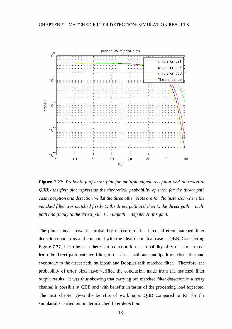
131


Figure 7.27: Probability of error plot for multiple signal reception and detection at

QBB:- the first plot represents the theoretical probability of error for the direct path

case reception and detection whilst the three other plots are for the instances where the

matched filter was matched firstly to the direct path and then to the direct path + multi

path and finally to the direct path + multipath + doppler shift signal.

The plots above show the probability of error for the three different matched filter

detection conditions and compared with the ideal theoretical case at QBB. Considering

Figure 7.27, it can be seen there is a reduction in the probability of error as one move

from the direct path matched filter, to the direct path and multipath matched filter and

eventually to the direct path, multipath and Doppler shift matched filter. Therefore, the

probability of error plots have verified the conclusion made from the matched filter

output results. It was thus showing that carrying out matched filter detection in a noisy

channel is possible at QBB and with benefits in terms of the processing load expected.

The next chapter gives the benefits of working at QBB compared to RF for the

simulations carried out under matched filter detection.

132


7.12 Benefits of carrying out matched filter detection at QBB

By now, from the previous chapters it has been shown how the processing load and

runtime for the simulations was measured. It was seen how the ratio of the amount of

processing correlated with the runtime ratios with reasonably small discrepancies

caused by the variance in the computer processing time. It was also seen that the

benefits were more for the real life case where the processing starts from baseband

itself. Therefore, for matched filtering case, the measurements for the runtimes and

calculations for the QBB case considered the real life scenario. In determining the

sample processing for the simulations, only the actual matched filtering stage was

considered with the signal generation procedures ignored and not being part of the

comparison process. The simulation runtime determination followed suit. The table

below summarises the outcome of the comparisons.


MF detection:-noiseless channel Time in seconds Ratio Number of

calculations Ratio

1. Direct path 0.01563 0.00372 4.20 2048 512 4.00

2. Multipath 0.01748 0.00461 3.79 2048 512 4.00

3. Doppler shift 0.01735 0.00444 3.91 2048 512 4.00

4. Multiple input 0.02925 0.00651 3.78 2048 512 4.00

MF detection :- noisy channel

1. Direct path 0.01568 0.00410 3.82 2048 512 4.00

2. Multiple input 0.04546 0.01203 4.11 6144 1536 4.00

Table 7.1: Simulation runtime and sample processing ratio comparisons. The highest

discrepancy between the ratios was about 5.8% which is reasonable given the slight

variance in the computer processing time. The amount of processing in terms of N for

the multiple signal input case for the noisy transmissions is three times more than that

for the direct path because of the 3 different matched filters used for the three

differently matched signals. The ratio however remains unaffected.

133


From the results obtained and shown in the table on the previous page, it does suffice to

conclude that matched filter detection at QBB is faster and less bulky in terms of

processor load than at RF. There were some limitations in defining some operations in

terms of N and therefore relevant assumptions were made so as to best show the

comparison between the processing at RF and that at QBB so as to correlate the

resulting ratio with that obtained for the simulation runtime. Again it should be noted

that the determination of the benefits interms of simulation runtime and sample

processing interms of N was just for analysis purposes and so as to see that indeed,

working at QBB is more advantageous.

7.13 Conclusion

The chapter looked at matched filter detection for various received signal scenarios and

considered noiseless and noisy transmissions. The matched filter output was larger for

multiple signal reception due to the matched filter locking on to the energies of the

individual input signals. For the detection in a noisy channel, the probability of error

plots showed a good correlation between the simulated and the theoretical probability of

error. The results obtained showed that working at QBB was not only possible but also

reduced the amount of sample processing due to the downsampling carried out. This in

turn reduced the simulation runtime. The discrepancies between the calculated and

simulated results were within reasonable limits and therefore, it does suffice to make a

firm conclusion that the benefits of working at QBB were indeed more than at RF in

terms of processing time and processing load.

134

Chapter 8

Conclusions This chapter concludes the study and gives an overview of the sample processing and

simulation runtime results for the whole study.

8.1 Conclusion The objectives of the study were achieved and it was verified that beamforming,

multipath compensation, Doppler shift compensation and the multiple compensation

special case and matched filter detection of a chirp signal (a) could take place at

quadrature baseband and (b) processing at quadrature baseband was more numerically

efficient which translated to less simulation runtimes. The various algorithms were

carried out at both RF and QBB and the results compared. It was seen under

beamforming that the results at QBB matched their corresponding RF counterparts and

so was the case for the multipath and Doppler shift cases. For the multiple input signal

case, there were some limitations in the compensation process but it was shown that

compensation was possible under certain conditions which were referred to as the

special case. Compensating for multipath and Doppler shift at quadrature baseband did

show that working at QBB facilitates sub-sampling which reduces the samples but does

not alter the information and hence the compensation process still proved a success.

The difference plots given after each of the compensation simulations did further

consolidate the effectiveness of the compensation process and thus acting as proof of

successful compensation. As already emphasised, working at quadrature baseband does

come with the main advantage of lower sampling frequencies which in-turn leads to less

complicated equipment and hence reducing operating costs. This study paves way for

further research into other signal processing techniques and the possibility of carrying

them out at QBB and hence this study is beneficial in that it would facilitate for the

enabling of most current signal processing techniques to be carried out at quadrature

baseband which comes with its core advantage of lower operating frequencies.

135

CHAPTER 8 – CONCLUSIONS

8.2 Summary of overall results

The overall results of the simulations carried out for whole study are summarised in the

table below. It was seen that operating at QBB did result in an overall improvement in

processing speed resulting from the reduction in samples by the downsampling process.

This was however not the case for the beamforming as it was seen that the amount of

processing required in the QBB case was more. The discrepancy range between the

sample processing and the simulation time ratios was from 1.5% to 5.8% and as

mentioned earlier, this was due to the variance in the computer processing runtime.


Beamforming Time in seconds Ratio Number of Calculations Ratio

AM DSB-SC 0.36318 0.74992 0.48 11776 25472 0.46

AM DSB-LC 0.35836 0.77418 0.46 11776 25472 0.46

Multipath Compensation

QAM 0.02715 0.01025 2.65 98304 37632 2.61

Doppler Shift Compensation

QAM 0.00119 0.00062 1.92 47104 24064 1.96

Multiple input:-Special case

QAM 0.00122 0.00099 1.23 67584 56832 1.19

Matched Filter(MF) Detection

Direct path 0.01563 0.00372 4.20 2048 512 4.00

Multipath 0.01748 0.00461 3.79 2048 512 4.00

Doppler shift 0.01735 0.00444 3.91 2048 512 4.00

Multiple input 0.02925 0.00651 3.78 2048 512 4.00

MF detection :-Noisy channel

Direct path 0.01568 0.00410 3.82 2048 512 4.00

Multiple input 0.04546 0.01203 4.11 6144 1536 4.00

Table 8.1: Summary of overall simulation results:- RF and QBB.

136

CHAPTER 8 – CONCLUSIONS

Finally, from the results, it was seen that working at lower QBB frequencies coupled

with its sub-sampling capabilities did indeed reduce the amount of processing required

which in turn led to a reduction in the simulation runtimes.

• For the beamforming case, the benefits of working at QBB were not felt in

terms number of calculations for the simulated QBB but when the real life case

of processing at baseband was considered the benefits were seen as the ratio of

the amount of processing at RF to that at QBB increased considerably by about

31 fold and thus entailing beamforming at QBB being much more efficient.

• For the multipath simulations, the amount of processing reduced by over 2-fold

for the simulated case and further reduced by about 9-fold for the real life case

showing the immense benefits of processing at QBB as compared to RF.

• For the Doppler shift case, the amount of processing reduced by less almost by

2-fold but upon taking up the processing from baseband itself for the real life

case as seen in chapter 5 there was approximately a 31 fold reduction which

showed that indeed, QBB does stand out in terms of processing benefits against

RF.

• The multiple compensation special case resulted in less reduction in processing

by operating at QBB but it still suffices to conclude that working at QBB was

more efficient.

• The matched filter detection showed a 4-fold reduction in processing load for

the real life QBB case which entails that carrying out the detection process at

QBB would result in less processing and hence when applied to real life digital

transmissions, it would entail much faster data rates, etc.

8.3 Future work The continued advancement in software defined radio technology entails the never

ending thirst for processing technologies that are compatible with the SDR equipment

and that enable more efficient use of available telecommunication resources such as

bandwidth. Therefore, this study focused on just a fragment of the many processing

techniques that would be required to be done at quadrature baseband considering the

benefits that come with it. Therefore, more research can be carried out into the

possibility of carrying out other processing techniques at QBB.

137

Bibliography

[1] J. Kirkhorn. ” Introduction to IQ demodulation of RF-data,” pp .4-10, EchoMAT

User Manual (FA292640), 15 September 1999.

[2] G-J van Rooyen and J.G. Lourens. ”A Quadrature Baseband Approach to Direct

Digital FM synthesis” pp. 228-229, IEEE Transactions on Broadcasting, Vol.46, NO 3 ,

September 2000.

[3] B.P. Lathi. ”Communication Systems,” Wiley and Sons, Inc, 1968.

[4] J.G. Proakis and M. Salehi. ”Communication Systems Engineering,” Prentice-Hall

International, Inc, 1994.

[5] “Signal Processing Toolbox User’s Guide-Version 4” pp 6-122 – 6-126, The

Mathworks, Inc, 1998.

[6] G-J van Rooyen. “Baseband Compensation Principles for Defects in Quadrature

Signal Conversion and Processing,” PhD Thesis, University of Stellenbosch, 2004.

[7] E.P. Cunningham. “Digital Filtering-An Introduction, “ John Wiley & Sons, inc,

1995.

[8] “Communications Toolbox User’s Guide -Version 1.3,” pp 3-65 – 3-67, The

Mathworks, Inc, 1996.

[9] V.K. Madisetti and D.B. Williams, “ The Digital Signal Processing Handbook,” 69-

1 -69-18, CRC press LCC, 1998.

[10] S. Haykin. “Adaptive Filter Theory”,2nd ed, Prentice-Hall, Englewood Cliffs, NJ,

1991.

[11] W.L. Stutzman and G.A. Thiele, “Antenna Theory and Design,” John Wiley and

Sons, Inc, 1998.

138

BIBLIOGRAPHY

[12] R. Kwok. “ AM modulation/demodulation,”

http://foe.mmu.edu.my/course/etm3046/notes/AM(-DSSC)ETM2042.doc

[13] H. Taub and D. L. Schilling. “Principles of Communication Systems,” pp 87 -131,

McGraw-Hill, inc, 1971.

[14] K.S. Shanmugam. ”Digital and Analog Communication systems,” John Wiley and

Sons,inc,1979.

[15] http://en.wikipedia.org/wiki/baseband

[16] P.B. Kenington. “RF and Baseband Techniques for Software Defined Radio,”

Artech house, Inc, 2005.

[17] W Tuttlebee. “Software defined radio,” John Wiley and Sons, Ltd 2002.

[18] C, Langton. “LTI and Matched Filter,” tutorial 21, 2003. www.complextoreal.com

,

[19] C.A Balanis. “Antenna theory,” 2nd edition, John Wiley & Sons Inc, 1982, 1997.

[20] ‘The digital signal processing handbook’,pp 68.2 -68.3,CRC press, LLC, 1992. [21] www.cisco.com/us/tech/tk722/multipath Document ID:27147

[22] L.R. Rabiner & B. Gold, “Theory and applications of DSP,“ prentice hall, Inc,

Bell Telephone laboratories and MIT Lincoln Libraries.1975

[23] J. H. Reed. “Software Radio-A modern approach to Radio Engineering” Prentice

Hall PTR, 2002.

[24] T . Niesler. “Digital Signal Processing notes,” SS 414 , slide 1.73 Stellenbosch

University, 2001-2008.

[25] http://en.wikipedia.org/wiki/Doppler_effect

139

BIBLIOGRAPHY

[26] H.L va Trees. “Detection,estimation and Modulation Theory,” part 3,Wiley, 2001

[27] S. W. Smith. “The scientist and Engineer’s Guide to Digital Signal Processing”,

www.dspguide.com/ch17/2.htm

[28] B, Gorid, R. Rabenstein and A.Stenger. “Signals and Systems,” John Wiley & Sons

Ltd, 2001.

[29].http://www.cambridge-en.com , Newsletter 5 -March 1999.html

[30] http://en.wikipedia.org/wiki/Chirp

[31] Mahafza, Bassem R. “Radar Systems Analysis and Design Using Matlab”

,Chapman &Hall/CRC, 2000.

[32] http://en.wikipedia.org/wiki/downsampling , 11/05/07.

[33] http://en.wikipedia.org/wiki/Envelope_detector , 9/04/07.

[34] http://en.wikipedia.org/wiki/Multiple-input_multiple-output , 6/3/07.

[35] H-S Lim, ”Benefits of FPGAs in Wireless Base Station Baseband Processing

Applications”, pp 1-10, XAPP726(v1.0) July,2005. www.xilinx.com

[36] http://www.agilent.com/find/mimo/ ,pp-6-11,application note 1509.

[37] B. Sklar. “Digital Communications Fundamentals and Applications,” Prentice

Hall, 1988.

[38] S. Haykin, “An Introduction to Analog and Digital Communications”, John

Wiley& Sons, Inc. 1989.

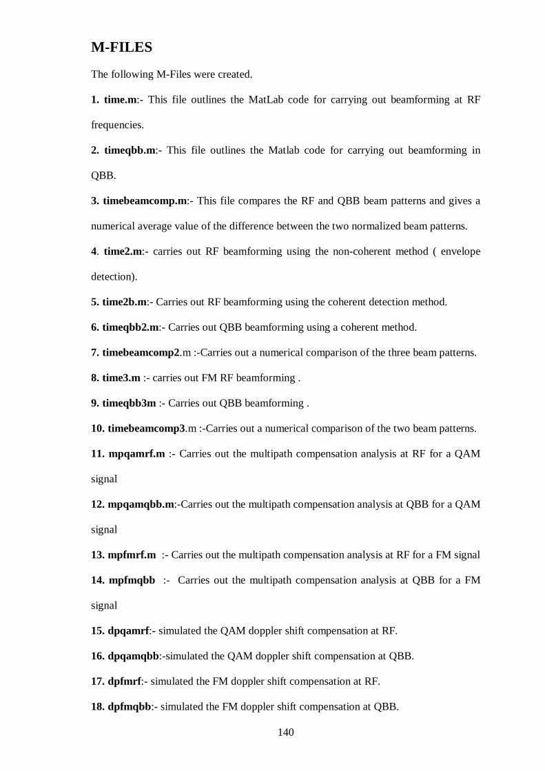
140

M-FILES The following M-Files were created. 1. time.m:- This file outlines the MatLab code for carrying out beamforming at RF

frequencies.

2. timeqbb.m:- This file outlines the Matlab code for carrying out beamforming in

QBB.

3. timebeamcomp.m:- This file compares the RF and QBB beam patterns and gives a

numerical average value of the difference between the two normalized beam patterns.

4. time2.m:- carries out RF beamforming using the non-coherent method ( envelope

detection).

5. time2b.m:- Carries out RF beamforming using the coherent detection method.

6. timeqbb2.m:- Carries out QBB beamforming using a coherent method.

7. timebeamcomp2.m :-Carries out a numerical comparison of the three beam patterns.

8. time3.m :- carries out FM RF beamforming .

9. timeqbb3m :- Carries out QBB beamforming .

10. timebeamcomp3.m :-Carries out a numerical comparison of the two beam patterns.

11. mpqamrf.m :- Carries out the multipath compensation analysis at RF for a QAM

signal

12. mpqamqbb.m:-Carries out the multipath compensation analysis at QBB for a QAM

signal

13. mpfmrf.m :- Carries out the multipath compensation analysis at RF for a FM signal

14. mpfmqbb :- Carries out the multipath compensation analysis at QBB for a FM

signal

15. dpqamrf:- simulated the QAM doppler shift compensation at RF.

16. dpqamqbb:-simulated the QAM doppler shift compensation at QBB.

17. dpfmrf:- simulated the FM doppler shift compensation at RF.

18. dpfmqbb:- simulated the FM doppler shift compensation at QBB.

141

M-FILES

19. mpdpqamrf.m:-Simulates the RF compensation process for the non-special case.

20. mpdpqamrf2.m:-Simulates the RF compensation process for the special case.

21. mpdpqamqbb.m:-Simulates the QBB compensation for the special case

22. chrf.m :- simulates the MF detection for the direct path signal at RF.

23. chqbb.m :- simulates the MF detection for the direct path signal at QBB.

24. chmprf.m :- simulates the MF detection for the multi-path signal at RF.

25. chmpqbb.m :- simulates the MF detection for the multi-path signal at QBB.

26. chdprf.m :- simulates the MF detection for the doppler-shift signal at RF.

27. chdpqbb.m :- simulates the MF detection for the doppler-shift signal at QBB.

28. chmpdprf.m :- simulates the MF detection for the multiple signal reception at RF.

29. chmpdpqbb.m :- simulates the MF detection for the multiple signal reception at QBB.

30. noiserf.m :- simulates the MF detection for the direct path signal at RF for a noisy channel.

31. noiseqbb.m :- simulates the MF detection for the direct path signal at QBB for a noisy channel.

32. mimonoiserf.m:- simulates the MF detection for the MIMO RF case for a noisy channel.

33. mimonoiseqbb.m:- simulates the MF detection for the MIMO QBB case for a noisy channel.

The M-files listed above were also re-run for the simulation time calculations too and

the processor load calculations for the simulations are included on the CD in Appendix

C.

142

Appendix A Theoretical derivation of probability of error

The derivation for the theoretical probability of error is given below. From the

mathematical analysis, the expected value of y(T) is 5.12e4 as shown in Chapter 7. We

now look at the noise power. In the simulation, the noise was multiplied by a variable

nch. Therefore we have:

{ }2 2oNo nch E xσ= = (A1)

The probability density function for a Gaussian distribution is given as

2

2

( )

2

2

1( )

2o

x m

o

f x e σ

πσ

− −

= (A2)

The expected value ‘m’ is the average of the value that a random variable takes in a

large number of experiments. The noise for the simulation is generated randomly using

‘randn’ and has a standard deviation of 1 because of the normal distribution [14, 18].

The noise power out numerical value is found using the following equations.

0

2| ( ) |outnoise op N nch H f df

−∞

= ∫ (A3)

which in the discrete domain is given as

1024

2

1

| ( ) |out

N

noise on

p N nch H n=

== ∑ (A4)

Inserting the limits of the integration leads us to the following expression in the discrete

domain:

1024

2

1

| ( ) | (5.12 4)out

N

noise o on

p N nch H n N nch e=

== =∑ (A5)

143

APPENDIX A – THEORETICAL DERIVATION OF PROBABILITY OF ERROR

The numerical value is substituted for |H(n)|2 because the absolute value of y(n) and

H(n) are the same. Referring back to equation A2, we can derive the expression for

the theoretical probability of error as follows:

2

2

( )0

2

2

1

2

x m

Pe e dxσ

πσ

− −

−∞

= ∫ (A6)

Let 2

x mt

σ− − =

then 2dx dtσ− = (A7)

The limits are equally changed due to the substitution gas shown below.

0,

2,

mx t

x tσ

→ →

→ −∞ → +∞ (A8)

Equation B6 then reduces to:

2 2

2

2

1 1m

t t

m

Pe e dt e dtσ

σ

π π

+∞− −

+∞

= − =∫ ∫ (A9)

Now MatLab does have an inbuilt command ‘erfc’ which executes the integral part of

equation B9 with the limits being positive.

erfc(x) = 22 t

x

e dtπ

+∞−

∫ (A10)

The outcome of the execution of this error function should give the same value as the

outcome of the same equation if it had its limits changed to negative values.

Therefore, the equation [37] can be re-written as:

Pe=2

2

1 t

m

e dt

σ

π

+∞−

∫ (A11)

144

APPENDIX A – THEORETICAL DERIVATION OF PROBABILITY OF ERROR

Written in terms of the MatLab error function, let a=2

m

σ we have:

Pe=1

( )2

erfc a (A12)

The values of m and σ are given below:

2

5.12 4

* | ( ) | (5.12 4)

m e

thus

nch h n nch eσ

=

= = (A13)

The theoretical Pe plot against the noise level in dBs was given earlier in Chapter 7 and

compared with the simulation plots. The actual values of the probability of error

theoretical and simulation plots obtained for at RF and QBB for the matched filter

detection in a noisy channel for the direct path case and multiple signal input case are

given in the Appendix C.

145

Appendix B

Model of a slowly fluctuating target

A slowly fluctuating target model for a radar/slowly fluctuating system is developed as follows;

Assume the sonar/radar system transmits a cosine wave continuously [26]. Thus;

( ) 2 cos( ) 2 Re[ ], .cj tt t c ts t P t Pe tωω= = −∞ < > ∞ (B1)

Now we assume a zero velocity target located at some range ‘R’ from the transmitter,

va Trees26 assumes that the target has a physical structure that includes several

reflecting surfaces. Thus the returned signal may be written as;

1

( ) 2 Re{ exp[ ( ) ]}K

r t i c ii

s t P g j tω τ θ=

= − +∑ (B2)

The attenuation gi includes the effects of the transmitting antenna gain. Assuming that

the reflection process is frequency-independent; thus if we transmit;

( ) 2 Re[ exp( )],t t cs t P j t j tω ω= + (B3)

We receive:

( ) 2 Re[ exp[( ( )( )]],r t cs t Pb j tω ω τ= + − (B4)

Assume a linear reflection process and considering a target with constant radial velocity

v and transmitted energy Et.. Further mathematical analysis leads us to the following

final expression below.

2 2

( ) 2 Re[ ( )exp[ ( )]].r c

v vs t Etbf t t j t t

c cτ ω= − + +ɶɶ (B5)

It is seen here that the target velocity has two effects which are;

1. A compression or stretching of the time scale of the complex envelope.

2. A shift of the carrier frequency.

146

APPENDIX C- MODEL OF SLOWLY MOVING TARGET

In most cases we can ignore this first effect. To demonstrate this, consider the error in

plotting ( )f tɶ instead of ( (2 / ) )f t v c t−ɶ . The maximum difference in the arguments

occurs at the end of the pulse (say T) and equals 2vT/c. The resulting error in amplitude

is a function of the signal bandwidth. If the signal bandwidth is W, the signal does not

change appreciably in a time equal to W-1 [26]. Therefore,

2 1vt

c W≪ (B6)

Or equivalently,

,2

cWT

v≪ (B7)

Ignoring the time-scale change, the shift in the carrier frequency is called the Doppler

shift.

2

( )D c

v

cω ω≜ (B8)

It should be noted that there some sonar problems in which Equation C8 is not satisfied.

In reality, we know that the speed of propagation of electromagnetic waves is very high

(3 x108) and therefore, the ratio given above will always be true in that the left hand

side will always be much greater than the RHS[26]. However, that is not the case for

acoustics propagation and therefore, the 1st part of our equation will have to be

considered.

147

Appendix C

Included CD

The CD included with this thesis contains the following

• The MatLab simulations and source code used to get the results in the thesis.

• The source code used in the simulation runtime and sample processing

calculations.

benefits to processor load for quadrature baseband versus radio

Documents