benefits derived from laser ranging measurements for orbit
TRANSCRIPT

Bryan W. Welch
Glenn Research Center, Cleveland, Ohio
Benefits Derived From Laser RangingMeasurements for Orbit Determinationof the GPS Satellite Orbit
NASA/TM—2007-214971
August 2007

NASA STI Program . . . in Profile
Since its founding, NASA has been dedicated to the
advancement of aeronautics and space science. The
NASA Scientific and Technical Information (STI)
program plays a key part in helping NASA maintain
this important role.
The NASA STI Program operates under the auspices
of the Agency Chief Information Officer. It collects,
organizes, provides for archiving, and disseminates
NASA’s STI. The NASA STI program provides access
to the NASA Aeronautics and Space Database and its
public interface, the NASA Technical Reports Server,
thus providing one of the largest collections of
aeronautical and space science STI in the world.
Results are published in both non-NASA channels and
by NASA in the NASA STI Report Series, which
includes the following report types:
• TECHNICAL PUBLICATION. Reports of
completed research or a major significant phase
of research that present the results of NASA
programs and include extensive data or theoretical
analysis. Includes compilations of significant
scientific and technical data and information
deemed to be of continuing reference value.
NASA counterpart of peer-reviewed formal
professional papers but has less stringent
limitations on manuscript length and extent of
graphic presentations.
• TECHNICAL MEMORANDUM. Scientific
and technical findings that are preliminary or
of specialized interest, e.g., quick release
reports, working papers, and bibliographies that
contain minimal annotation. Does not contain
extensive analysis.
• CONTRACTOR REPORT. Scientific and
technical findings by NASA-sponsored
contractors and grantees.
• CONFERENCE PUBLICATION. Collected
papers from scientific and technical
conferences, symposia, seminars, or other
meetings sponsored or cosponsored by NASA.
• SPECIAL PUBLICATION. Scientific,
technical, or historical information from
NASA programs, projects, and missions, often
concerned with subjects having substantial
public interest.
• TECHNICAL TRANSLATION. English-
language translations of foreign scientific and
technical material pertinent to NASA’s mission.
Specialized services also include creating custom
thesauri, building customized databases, organizing
and publishing research results.
For more information about the NASA STI
program, see the following:
• Access the NASA STI program home page at
http://www.sti.nasa.gov
• E-mail your question via the Internet to
• Fax your question to the NASA STI Help Desk
at 301–621–0134
• Telephone the NASA STI Help Desk at
301–621–0390
• Write to:
NASA Center for AeroSpace Information (CASI)
7115 Standard Drive
Hanover, MD 21076–1320

Bryan W. Welch
Glenn Research Center, Cleveland, Ohio
Benefits Derived From Laser RangingMeasurements for Orbit Determinationof the GPS Satellite Orbit
NASA/TM—2007-214971
August 2007
National Aeronautics and
Space Administration
Glenn Research Center
Cleveland, Ohio 44135
Prepared for the
63rd Annual Meeting
sponsored by the Institue of Navigation (ION)
Cambridge, Massachusetts, April 23–25, 2007

Acknowledgments
The author would like to thank the Space Communications Architecture Working Group for providing a forum to develop the orbit
determination navigation analysis tools, and the opportunity to contribute to the analysis a comparison of utilizing radiometric
versus radiometric/laser measurements for orbit determination of a GPS satellite orbit.
This work was performed at the NASA Glenn Research Center in Cleveland, Ohio, with funding being provided by the NASA
Space Operations Mission Directorate Space Communication and Navigation Project.
Available from
NASA Center for Aerospace Information
7115 Standard Drive
Hanover, MD 21076–1320
National Technical Information Service
5285 Port Royal Road
Springfield, VA 22161
Available electronically at http://gltrs.grc.nasa.gov
Level of Review: This material has been technically reviewed by technical management.
This report contains preliminary findings,
subject to revision as analysis proceeds.

NASA/TM—2007-214971 1
Benefits Derived From Laser Ranging Measurements for Orbit Determination of the GPS Satellite Orbit
Bryan W. Welch
National Aeronautics and Space Administration Glenn Research Center Cleveland, Ohio 44135
Abstract While navigation systems for the determination of the orbit
of the Global Position System (GPS) have proven to be very effective, the current research is examining methods to lower the error in the GPS satellite ephemerides below their current level. Two GPS satellites that are currently in orbit carry retro-reflectors onboard. One notion to reduce the error in the satellite ephemerides is to utilize the retro-reflectors via laser ranging measurements taken from multiple Earth ground stations. Analysis has been performed to determine the level of reduction in the semi-major axis covariance of the GPS satellites, when laser ranging measurements are supplemented to the radiometric station keeping, which the satellites undergo.
Six ground tracking systems are studied to estimate the performance of the satellite. The first system is the baseline current system approach which provides pseudo-range and integrated Doppler measurements from six ground stations. The remaining five ground tracking systems utilize all measurements from the current system and laser ranging measurements from the additional ground stations utilized within those systems. Station locations for the additional ground sites were taken from a listing of laser ranging ground stations from the International Laser Ranging Service.
Results show reductions in state covariance estimates when utilizing laser ranging measurements to solve for the satellite’s position component of the state vector. Results also show dependency on the number of ground stations providing laser ranging measurements, orientation of the satellite to the ground stations, and the initial covariance of the satellite’s state vector.
Introduction The task of the laser ranging analysis effort was to deter-
mine the added benefits derived from solving for a space-craft’s state vector when utilizing laser ranging measurements in addition to the current use of pseudo-range and accumulated delta range (ADR), also known as Integrated Doppler measurements. The methodology to complete this analysis is to perform a covariance study for the Global Positioning System (GPS) orbit. The definition for this study of added benefits was a reduction in the covariance estimate of the GPS
orbit state vector. The exact covariance statistic that was examined will be discussed in a later section.
Two methods were utilized in this study for the purposes of estimating benefits of laser ranging measurements being applied in solving for the GPS orbit state vector. The first method was to perform the estimated orbit determination (OD) using pseudo-range and ADR measurements from the six Monitor Stations (MS) for the GPS satellite orbit through an Extended Kalman Filter (EKF) analysis. The second method also used the EKF analysis tool, but included laser ranging measurements from the six MS sites along with various amounts of additional sites. Measurements from both methods were used to form estimates for the GPS satellite’s state vector, which was propagated until new measurements were available. Finally, comparisons were made between the performance of the current system and the modified system.
This analysis is intended to be the baseline study comparing the benefits of adding laser ranging measurements from various numbers of ground stations. This analysis is not meant to reflect on operational scenarios, nor provide a baseline operational concept. This analysis is meant to provide inform-ation on the benefits of having multiple ground stations in view while providing laser ranging measurements, in compari-son to the current system which uses pseudo-range (PR) and Accumulated Delta Range (a.k.a. Integrated Doppler) (ADR) measurements.
EKF Description The purpose of an EKF is to estimate the states of a non-linear
system. The EKF is an extension of the standard Kalman Filter, in which its purpose is to estimate the states of a linear system. The derivation of the EKF is based on linearizing the non-linear system using the Kalman Filter estimate as the nominal state trajectory. The non-linear system is linearized around the Kalman Filter estimate and the Kalman Filter estimate is based on the linearized system (ref. 1).
The method of the EKF used for these simulations was the discrete time system/discrete time measurement EKF. This was the most appropriate method to simulate the EKF because performing continuous time dynamics on a computer requires an extremely large amount of memory and processor power to be performed efficiently. Also, it is important to note initially that there are multiple runs performed for each scenario. This

NASA/TM—2007-214971 2
is due to the fact that the equations of the EKF dictate that the real noise parameters, instead of the covariance of the noise (as in linear Kalman filter problems), be used to form new estimates of the state estimates. The dictating equations for the EKF process can be found in reference one.
State Dynamics Description The orbit of the GPS satellite was viewed as a simplified
two-body problem for this analysis. Therefore, the differential equation that solves the two-body problem is as follows, in equation (1) (ref. 2).
darR
r =μ
+3
(1)
Where:
r is the position matrix r is the 2nd time derivative of the position matrix μ is the Earth’s Gravitational constant R is the magnitude of the position matrix
da is the orbital perturbation
It is important to note that the OD analysis solved for more than just the position matrix. The purpose of the OD analysis was to solve for position, velocity, clock bias, and frequency bias estimates. Therefore, the state equation that governed the OD analysis was an extension of the two-body problem. Keep in consideration that the orbital perturbation was assumed to be zero for this analysis. The state is defined in equation (2), while the state equation is given as follows in equation (3).
⎥⎥⎥⎥
⎦
⎤
⎢⎢⎢⎢
⎣
⎡
=
bias
bias
tcct
vr
x (2)
w
f
xR
v
x⎥⎥⎥⎥
⎦
⎤
⎢⎢⎢⎢
⎣
⎡
+
⎥⎥⎥⎥⎥
⎦
⎤
⎢⎢⎢⎢⎢
⎣
⎡μ−
=
/1100
00
3 (3)
Where: r is the position matrix v is the velocity matrix c is the speed of light in a vacuum
biast is the clock difference between the satellite and the ground stations
f is the GPS L1 frequency w is the state noise
⎥⎥⎥⎥⎥⎥⎥⎥⎥⎥⎥
⎦
⎤
⎢⎢⎢⎢⎢⎢⎢⎢⎢⎢⎢
⎣
⎡
=
⎥⎥⎥⎥⎥⎥⎥⎥⎥⎥⎥
⎦
⎤
⎢⎢⎢⎢⎢⎢⎢⎢⎢⎢⎢
⎣
⎡
=
bias
bias
zk
yk
xk
zk
yk
xk
k
k
k
k
k
k
k
k
k
tcctvvvrrr
xxxxxxxx
x
,
,
,
,
,
,
8,
7,
6,
5,
4,
3,
2,
1,
(4)
Equation (4) shows the fully expanded form of the discrete
state equation. Equation (5) converts the state equation from equation (3) into a discrete time state equation, needed for the discrete time EKF, in Earth-Centered Fixed coordinates. Where:
φ is the Earth rotation rate in radians/second Δ is the discrete time step
( ) ( ) ( ) ( )( ) ( ) ( ) ( )
( ) ( ) ( ) ( )
( ) ( ) ( ) ( ) kkk w
f
x
R
RR
RRx
⎥⎥⎥⎥⎥⎥⎥⎥⎥⎥⎥
⎦
⎤
⎢⎢⎢⎢⎢⎢⎢⎢⎢⎢⎢
⎣
⎡
+
⎥⎥⎥⎥⎥⎥⎥⎥⎥⎥⎥⎥⎥
⎦
⎤
⎢⎢⎢⎢⎢⎢⎢⎢⎢⎢⎢⎢⎢
⎣
⎡
μ−
φφ−φμ
−φμ
φφφμ
−φμ
−
ΔφΔφΔ−φφ−φΔφΔφφ
=+
/11000000
1000000001000000
0010000
000cossin0cossin
000sincos0sincos0000100000cossin0cossin000sincos0sincos
3
33
33
1 (5)

NASA/TM—2007-214971 3
Measurement Description There are three different measurement types that were
utilized within the trade space of this analysis. The first measurement was the pseudo-range (PR) measurement, which was utilized at the MS locations. The equation for the pseudo-range measurement is given in equation (6) (ref. 3).
( ) ( ) ( )PRbias vct
zzyyxxPR++
−+−+−= 221
221
221 (6)
Where:
PR is the pseudo-range measurement ( )111 ,, zyx was the position of the transmitter (or receiver) ( )222 ,, zyx was the position of the receiver (or transmitter)
PRv was the noise term in the pseudo-range measurement
The second measurement type that was utilized at the six MS locations was the Accumulated Delta Range (ADR) measurement. This measurement, which is also called carrier phase, is the integral of the range-rate measurement used with instantaneous Doppler shift. Equation (7) provides the mathematical description of the ADR measurement (ref. 3).
( ) ( )( ) ( )( ) ( )}( ) ( ) ( )
]ADRbias
n
i
vtfc
kzkzkykykxkx
kvzkvzkzkzkvykvykyky
kvxkvxkxkxADR
++
−+−+−
−−+
−−+
⎢⎣⎡⎩⎨⎧ −−= ∑
=
222
0
,2,1,2,1,2,1
,2,1,2,1
,2,1,2,1
,2,1,2,1
(7)
Where:
ADR was the accumulated delta range measurement ( )111 ,, vzvyvx was the velocity of the transmitter (or re-
ceiver) ( )222 ,, vzvyvx was the velocity of the receiver (or trans-
mitter) ADRv was the noise term in the accumulated delta range
measurement
The final measurement type which was utilized only in the modified systems, but at all ground station sites, was the laser ranging (LR) measurement. This was thought of as the equivalent of a two-way radiometric signal, in terms of the equation governing the measurement. Equation (8) provides the mathematical description of the LR measurement (ref. 3).
( ) ( ) ( ) LRvzzyyxxLR +−+−+−= 221
221
221 (8)
Where: LR was the laser ranging measurement
LRv was the noise term in the laser ranging measurement
Table 1 provides the standard deviation of the noise terms that are assumed for the three measurement equations provided in equations (6) through (8). TABLE 1.—MEASUREMENT NOISE STANDARD DEVIATION
Noise term PRv ADRv LRv σ 2 m 5 mm/s 1 m
Station Locations The first of the two proposed systems that were analyzed
was the current system (CS), which utilized pseudo-range and ADR measurements from the six MS locations. The second proposed system was the modified system, from which there were five versions (MSys1, MSys2, MSys3, MSys4, and MSys5). The modified system utilized all measurements for the current system, plus laser ranging measurements from the six MS locations along with measurements from various additional ground stations present in each system. The locations of the additional ground stations are from a listing of laser ranging sites from the International Laser Ranging Service (ref. 4). Figure 1 illustrates the locations of all of the ground station locations with color coded dots representing which system the ground stations are first utilized within on a Mercator projection of the Earth’s surface. Blue dots represent the six MS ground stations. Red dots represent the two sites first utilized in MSys1. Orange dots represent the two sites first utilized in MSys2. Green dots represent the four sites first utilized in MSys3. Pink dots represent the four sites first utilized in MSys4. Finally, purple dots represent the four sites utilized in MSys5. Table 2 provides an alphabetical listing of the all 22 ground stations locations utilized in the study and which systems they were part of.
Figure 1.—Ground station location map.

NASA/TM—2007-214971 4
TABLE 2.—GROUND STATIONS
Station CS
MSy
s1
MSy
s2
MSy
s3
MSy
s4
MSy
s5
Arequipa X Ascension Island X X X X X X Cape Canaveral X X X X X X Colorado Springs X X X X X X Concepcion X X X Diego Garcia X X X X X X Greenbelt X X X X X Hartebeesthoek X X X X Hawaii X X X X X X Koganei X Komsomolsk X X X Kwajalein X X X X X X McDonald Obs. X X X X X Metsahovi X X X Mt. Stromlo X X X Riyadh X San Fernando X X Tahiti X X Urumqi X X Wrightwood X Wuhan X X X X Yarragadee X X
Methodology Description This analysis was performed using the discrete
time/discrete measurement EKF procedure described previ-ously. The state was propagated at a rate of 1 Hz. The total simulation was set to run for 1 day (86400 s). It should be noted however, that measurements were not taken on this same one second time period.
The instant that line-of-sight was available, the pseudo-range measurements were recorded at the ground station and again every 60 s after the initial measurement, until the ground station was no longer visible to the satellite.
For ADR measurements, the integration of the delta-range measurements began the first second that the ground station was visible to the satellite. The measurement was completed once the ground station had been in view for 60 s. When the satellite lost visibility to the ground station, the integration procedure was reset and the measurement integration process had to start over on the next visible pass.
Laser ranging measurements were recorded at the ground station the instant that the ground station was visible to the satellite, and again every 60 s after the initial measurement, until the satellite was no longer visible to the ground station.
Note that in order for the ground station to be visible to the satellite, or for the satellite to be visible to the ground station, the ground station must see the satellite with an elevation angle of 10° minimum. This rule applied to all three measure-ment types that have been described.
The satellite was modeled in the GPS 12 hr orbit at an inclination of 55°. The orbit was assumed to start on the plane
of the Earth’s Equator. However, due to the nature that the ground stations were oriented on the surface, the satellite was modeled on starting longitudes of 0° and 90° E. Figures 2 and 3 show the points over the Earth surface (Mercator projection) in which the orbit for these two starting longitudes pass. Note that the point shown in red was the first point of the orbit in the simulation.
Initial errors on the order of 1 km were added to each Cartesian dimension along with 1 m/s velocity errors in each Cartesian dimension. Clock bias and frequency bias states also begin with a 1 km and 1 m/s error, respectively. The other condition that was varied for the simulation was the initial covariance estimate. Initial conditions for the covariance estimate are formed into nine cases, as listed in table 3.
Finally, for the purpose of this analysis, there were 10 noise profile runs performed for every starting longitude/initial covariance case simulation. Performance along the multiple runs will be combined to attain overall performance.
Figure 2.—Satellite ground path—starting longitude 0°.
Figure 3.—Satellite ground path—starting longitude 90°.

NASA/TM—2007-214971 5
TABLE 3.—INITIAL COVARIANCE CONDITIONS Case Position,
m2 Velocity,
(m/s)2 1 0.1 0.1 2 0.1 1 3 0.1 10 4 1 0.1 5 1 1 6 1 10 7 10 0.1 8 10 1 9 10 10
Results Results for the analysis of the comparison of the six systems
are shown through the use of the covariance estimate of the systems. Even though the variance of the noise terms is constant throughout the simulations, multiple noise profiles are needed to analyze the performance of an EKF simulation. This is due to the fact that the equations of the EKF dictate that the real noise parameters, instead of the covariance of the noise, are used to form new estimates of the state. The metric to compare the performance of the six systems was semi-major axis (SMA) covariance, which was based on the final covariance estimate at the end of the simulation.
Equation (9) was used to compare the systems for the SMA covariance statistic for the covariance estimate.
∑ ∑= =
++
=
nlong
i
nrun
iiiiikfiiikfiiikf
SMA
PPP
nrunnlongCOV
1 1,,),3,3(2,,),2,2(2,,),1,1(2
**1
(9)
Where: SMACOV was the semi-major axis covariance error from the covariance estimate
( )iiikfiiikfiiikf PPP ,,),3,3(,,),2,2(,,),1,1( ,, were the covariance terms for the individual Cartesian dimension position terms at final time kf for run ii at longitude case i
nlong was the number of starting longitude scenarios nrun was the number of noise profile runs
There will be a bar graph that corresponds to the final time SMA covariance statistic calculated by equation (9). Plots will illustrate the non-averaged SMA covariance statistic over time for all of the noise profiles for each of the systems that were examined, for the nine initial covariance estimates, respec-tively. Each figure has a top and bottom subplot, correspond-ing to the 0° and 90° E starting longitude conditions. Line color corresponds to systems in the following manner:
• Blue—CS • Red—Msys1 • Black—MSys2
• Green—MSys3 • Cyan—MSys4 • Yellow—MSys5
Figures 4 and 5 correspond to the results for the initial covari-
ance Case 1 simulations with initial covariance parameters are on the order of 0.1 m2 and 0.1 (m/s)2.
Figure 4.—Final time SMA covariance—Case 1.
Figure 5.—SMA covariance—Case 1.

NASA/TM—2007-214971 6
Figures 6 and 7 correspond to the results for the initial covariance Case 2 simulations with initial covariance parame-ters are on the order of 0.1 m2 and 1 (m/s)2.
Figure 6.—Final time SMA covariance—Case 2.
Figure 7.—SMA covariance—Case 2.
Figures 8 and 9 correspond to the results for the initial covariance Case 3 simulations with initial covariance parame-ters are on the order of 0.1 m2 and 10 (m/s)2.
Figure 8.—Final time SMA covariance—Case 3.
Figure 9.—SMA covariance—Case 3.

NASA/TM—2007-214971 7
Figures 10 and 11 correspond to the results for the initial covariance Case 4 simulations with initial covariance parame-ters are on the order of 1 m2 and 0.1 (m/s)2.
Figure 10.—Final time SMA covariance—Case 4.
Figure 11.—SMA covariance—Case 4.
Figures 12 and 13 correspond to the results for the initial covariance Case 5 simulations with initial covariance parame-ters are on the order of 1 m2 and 1 (m/s)2.
Figure 12.—Final time SMA covariance—Case 5.
Figure 13.—SMA covariance—Case 5.

NASA/TM—2007-214971 8
Figures 14 and 15 correspond to the results for the initial covariance Case 6 simulations with initial covariance parame-ters are on the order of 1 m2 and 10 (m/s)2.
Figure 14.—Final time SMA covariance—Case 6.
Figure 15.—SMA covariance—Case 6.
Figures 16 and 17 correspond to the results for the initial covariance Case 7 simulations with initial covariance parame-ters are on the order of 10 m2 and 0.1 (m/s)2.
Figure 16.—Final time SMA covariance—Case 7.
Figure 17.—SMA covariance—Case 7.
NASA/TM—2007-214971 9
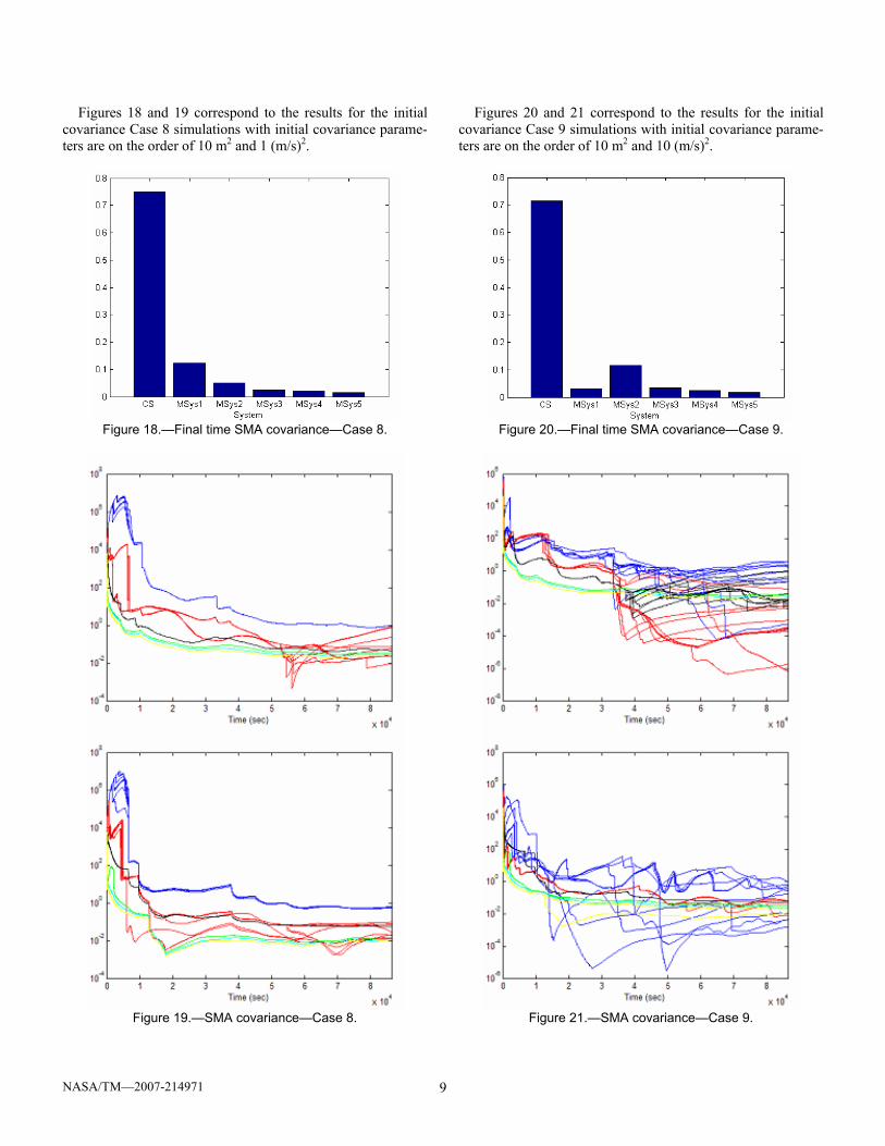
Figures 18 and 19 correspond to the results for the initial covariance Case 8 simulations with initial covariance parame-ters are on the order of 10 m2 and 1 (m/s)2.
Figure 18.—Final time SMA covariance—Case 8.
Figure 19.—SMA covariance—Case 8.
Figures 20 and 21 correspond to the results for the initial covariance Case 9 simulations with initial covariance parame-ters are on the order of 10 m2 and 10 (m/s)2.
Figure 20.—Final time SMA covariance—Case 9.
Figure 21.—SMA covariance—Case 9.

NASA/TM—2007-214971 10
It is important to notice how the starting longitude and initial starting covariance affect the performance for each of the systems. Starting longitude will change which stations are visible, and if there are fewer stations visible, then the covariance estimate will grow at a faster rate between measurements. Initial covariance cases in which the velocity terms have a lower or equal initial covariance than the position terms perform more consistently, compared to the opposite case when the velocity terms have larger initial covariance terms than the position terms. This is due to the fact that the position error grows faster as position is the integral of velocity. Table 4 provides the final time percentage of the SMA covariance of the five systems compared to the SMA covariance of the current system, averaged over all initial covariance/initial longitude/noise profile runs. Note that these values represent the percentage of the CS SMA covariance of the five different systems.
TABLE 4.—SMA COVARIANCE PERCENTAGE RESULTS System MSys1 MSys2 MSys3 MSys4 MSys5 Results 14.13% 11.01% 5.03% 3.84% 3.03%
Conclusion Results for the comparison between the current tracking
system utilizing pseudo-range and ADR measurements from the six MS locations with the five modified systems including laser ranging measurements from the same ground sites plus additional sites have been provided. All of the results show benefits of having laser ranging measurements used to solve for the satellite’s position component of the state vector. The results show an initial dependency on the initial longitude of the orbit. A second parameter that has been shown to affect performance is the initial covariance for the system. However, for both of these parameters, the final SMA covariance is not strongly affected.
The parameter that does strongly affect the final time co-variance is the number of laser ranging ground stations used. As seen in the results, it is typical that with an increase in the number of laser ranging ground stations, the final time SMA covariance statistic decreases. It is important to note that as more and more ground stations are added to the scenario, the final time covariance does not keep decreasing forever, but appears to reach a lower bound.
The initial covariance of the state is an estimate for how well the state is understood. Typically, when the state’s covariance is larger, then more emphasis is placed on the measurements when producing the EKF Kalman gain. The covariance of the measurement noise is also an important parameter for how the state covariance is propagated. However, when dealing with an OD type of analysis similar to the one performed, where and when there are few measure-ments available to the receiver, then covariance parameters can increase quickly.
Results shown from this study include the fact that there are differences in performance between the current system and the
modified systems including laser ranging measurements. Performance is dependent on the location of the ground stations and how those stations are viewed by the satellite. Therefore, if the additional ground stations for the modified systems were picked differently, then the results would vary. However, this issue is not viewed to significantly modify the results as laser ranging ground stations were selected to be spatially diverse. It is believed that if constraints (such as range and/or speed) are placed within the EKF, performance of the two systems may be better modeled.
This analysis has shown that laser ranging measurements are beneficial and reduce the steady state system performance. Typically, the more stations that are added to the scenario, the lower the steady state system performance will be. MSys3 provides SMA covariance results of 5.03% of the CS results. MSys4 provides SMA covariance of 3.84% of the CS results. MSys5 provides SMA covariance of 3.03% of the CS results. However, there are smaller reductions in SMA covariance when comparing MSys3 to MSys4 or MSys4 to MSys5. Therefore, given the orientation of the ground stations as such as in this report, it appears that MSys3 would give the most benefit. Therefore, it is believed that if laser ranging meas-urements would in the future be taken into account for doing orbit determination analysis on a GPS orbit, the recommenda-tion would be have measurements taken from the six MS stations with measurements from an additional eight ground stations around the world.
References 1. Dan Simon, Optimal State Estimation, John Wiley & Sons, 2006. 2. James R Wertz and Wiley J. Larson, Space Mission Analysis and
Design, Microcosm Press, 1999. 3. Mohinder S. Grewal, Lawrence R. Weill, & Angus P. Andrews,
Global Positioning Systems, Inertial Navigation and Integration, John Wiley & Sons, 2001.
4. International Laser Ranging Service, http://ilrs.gsfc.nasa.gov/, August 2006.
Biography Bryan W. Welch is a member of the Communication Sys-
tem Integration Branch of the Communications Technology Division at the National Aeronautics and Space Administra-tion's Glenn Research Center at Lewis Field in Cleveland, Ohio. Mr. Welch earned his Bachelor’s of Science Degree in Electrical Engineering from Cleveland State University, graduating summa cum laude in May 2003. In 2006, Mr. Welch earned his Master’s Degree in Electrical Engineering, also at Cleveland State University, with his thesis topic on the utilization of the Ruze Equation for inflatable aperture antennas. He has coauthored many papers, including some presented at the 4th ICNS Conference in April 2004, the ION National Technical Meeting in January 2006, and the Ka Band Conference in September 2006.

REPORT DOCUMENTATION PAGE Form Approved OMB No. 0704-0188
The public reporting burden for this collection of information is estimated to average 1 hour per response, including the time for reviewing instructions, searching existing data sources, gathering and maintaining the data needed, and completing and reviewing the collection of information. Send comments regarding this burden estimate or any other aspect of this collection of information, including suggestions for reducing this burden, to Department of Defense, Washington Headquarters Services, Directorate for Information Operations and Reports (0704-0188), 1215 Jefferson Davis Highway, Suite 1204, Arlington, VA 22202-4302. Respondents should be aware that notwithstanding any other provision of law, no person shall be subject to any penalty for failing to comply with a collection of information if it does not display a currently valid OMB control number. PLEASE DO NOT RETURN YOUR FORM TO THE ABOVE ADDRESS. 1. REPORT DATE (DD-MM-YYYY) 01-08-2007
2. REPORT TYPE Technical Memorandum
3. DATES COVERED (From - To)
4. TITLE AND SUBTITLE Benefits Derived From Laser Ranging Measurements for Orbit Determination of the GPS Satellite Orbit
5a. CONTRACT NUMBER
5b. GRANT NUMBER
5c. PROGRAM ELEMENT NUMBER
6. AUTHOR(S) Welch, Bryan, W.
5d. PROJECT NUMBER
5e. TASK NUMBER
5f. WORK UNIT NUMBER WBS 439432.07.04.03.01
7. PERFORMING ORGANIZATION NAME(S) AND ADDRESS(ES) National Aeronautics and Space Administration John H. Glenn Research Center at Lewis Field Cleveland, Ohio 44135-3191
8. PERFORMING ORGANIZATION REPORT NUMBER E-16125
9. SPONSORING/MONITORING AGENCY NAME(S) AND ADDRESS(ES) National Aeronautics and Space Administration Washington, DC 20546-0001
10. SPONSORING/MONITORS ACRONYM(S) NASA
11. SPONSORING/MONITORING REPORT NUMBER NASA/TM-2007-214971
12. DISTRIBUTION/AVAILABILITY STATEMENT Unclassified-Unlimited Subject Category: 17 Available electronically at http://gltrs.grc.nasa.gov This publication is available from the NASA Center for AeroSpace Information, 301-621-0390
13. SUPPLEMENTARY NOTES
14. ABSTRACT While navigation systems for the determination of the orbit of the Global Position System (GPS) have proven to be very effective, the current research is examining methods to lower the error in the GPS satellite ephemerides below their current level. Two GPS satellites that are currently in orbit carry retro-reflectors onboard. One notion to reduce the error in the satellite ephemerides is to utilize the retro-reflectors via laser ranging measurements taken from multiple Earth ground stations. Analysis has been performed to determine the level of reduction in the semi-major axis covariance of the GPS satellites, when laser ranging measurements are supplemented to the radiometric station keeping, which the satellites undergo. Six ground tracking systems are studied to estimate the performance of the satellite. The first system is the baseline current system approach which provides pseudo-range and integrated Doppler measurements from six ground stations. The remaining five ground tracking systems utilize all measurements from the current system and laser ranging measurements from the additional ground stations utilized within those systems. Station locations for the additional ground sites were taken from a listing of laser ranging ground stations from the International Laser Ranging Service. Results show reductions in state covariance estimates when utilizing laser ranging measurements to solve for the satellite’s position component of the state vector. Results also show dependency on the number of ground stations providing laser ranging measurements, orientation of the satellite to the ground stations, and the initial covariance of the satellite’s state vector. 15. SUBJECT TERMS Global positioning system; Navigation; Space navigation; Positioning; Orbit determination; State estimation; Kalman filters; Satellite laser ranging; Laser ranging
16. SECURITY CLASSIFICATION OF: 17. LIMITATION OF ABSTRACT UU
18. NUMBER OF PAGES
16
19a. NAME OF RESPONSIBLE PERSON STI Help Desk (email:[email protected])
a. REPORT U
b. ABSTRACT U
c. THIS PAGE U
19b. TELEPHONE NUMBER (include area code) 301-621-0390
Standard Form 298 (Rev. 8-98)Prescribed by ANSI Std. Z39-18

