Benchmarking Low-Volatility Strategies

David Blitz*

Head Quantitative Equity Research

Robeco Asset Management

Pim van Vliet, PhD**

Portfolio Manager Quantitative Equity

Robeco Asset Management

forthcoming Journal of Index Investing

February 2011

* Coolsingel 120, 3011 AG Rotterdam, The Netherlands, tel. +31 10 224 2079, e-mail d.c.blitz@robeco.com

(corresponding author)

** Coolsingel 120, 3011 AG Rotterdam, The Netherlands, tel. +31 10 224 2579, e-mail p.van.vliet@robeco.com

1

Abstract

In this paper we discuss the benchmarking of low-volatility investment strategies,

which are designed to benefit from the empirical result that low-risk stocks tend

to earn high risk-adjusted returns. Although the minimum-variance portfolio of

Markowitz is the ultimate low-volatility portfolio, we argue that it is not a suitable

benchmark, as it can only be determined with hindsight. This problem is

overcome by investable minimum-variance strategies, but because various

approaches are equally effective at minimizing volatility it is ambiguous to elevate

the status of any one particular approach to benchmark. As an example we

discuss the recently introduced MSCI Minimum Volatility indices and conclude

that these essentially resemble active low-volatility investment strategies

themselves, rather than a natural benchmark for such strategies. In order to

avoid these issues, we recommend to simply benchmark low-volatility managers

against the capitalization-weighted market portfolio, using risk-adjusted

performance metrics such as Sharpe ratio or Jensen’s alpha.

2

1. Introduction

Low-risk stocks tend to earn high risk-adjusted returns. This stylized fact was first

established by Black, Jensen and Scholes (1972) and Fama and MacBeth

(1973), whose empirical tests of the Capital Asset Pricing Model (CAPM) showed

that the relation between beta and return in the U.S. stock market is flatter than

predicted by theory. This effect does not appear to have weakened over time,

does not depend critically on the choice of risk measure (e.g. volatility instead of

beta) or risk calculation method (e.g. 3- or 5-year trailing data) and has also been

confirmed for international markets; see Fama and French (1992), Black (1993),

Falkenstein (1994), Blitz and Van Vliet (2007) and Baker, Bradley, and Wurgler

(2010). These studies suggest that the empirical relation between volatility and

return in the equity market is flat or negative, a phenomenon which throughout

this paper we will refer to as “the volatility effect”.

The studies above consider quantile portfolios based on a ranking of the

universe of stocks on risk measures such as past volatility or beta. Further

support for the existence of a volatility effect is provided by a related stream of

literature, which uses mean/variance optimization to determine the portfolio with

minimum past volatility, see for example Haugen and Baker (1991) and Clarke,

de Silva and Thorley (2006).1 Although these authors use a more sophisticated

technique to construct low-volatility portfolios (for example, optimization also

takes into account correlation effects), their conclusions are similar: portfolio

volatility can be reduced significantly without negative implications for expected

returns.

To summarize, the literature reports a persistent volatility effect, which

appears to be robust to research design choices with regard to sample period,

universe and portfolio construction methodology. Attracted by these findings, an

increasing number of investors have adopted low-volatility investment strategies

in recent years. One of the questions which arises as a result of this trend is how

to evaluate the performance of low-volatility managers in practice. 1 Examples of other low-volatility portfolio construction techniques that have been proposed are “equally-weighted risk contribution” portfolios, see Maillard, Roncalli and Teiletche (2010), and “most diversified” portfolios, see Choueifaty and Coignard (2008).

3

The first thought that may come to mind is to simply benchmark low-

volatility managers against an appropriate low-volatility index. However, we

argue that this is not as straightforward as it may seem. To begin with, a

benchmark should represent an investable alternative. This disqualifies the

unique minimum-variance portfolio that exists in theory, as it is not observable ex

ante. Investable approximations to the true minimum-variance portfolio may be

considered instead, but here the problem is that various approaches appear to

be equally valid, implying that it is arbitrary to elevate the status of any one

particular approach to benchmark for all low-volatility strategies. As an example

we discuss the recently introduced MSCI Minimum Volatility indices, concluding

that these essentially resemble active low-volatility investment strategies

themselves, rather than providing a benchmark for the entire class of low-

volatility strategies. Although a comparison between the performance of a low-

volatility manager and a minimum-volatility index may be informative, a more

general and universally applicable method is to be preferred. We propose to

simply benchmark low-volatility managers against the capitalization-weighted

market portfolio, using established risk-adjusted performance metrics such as

Sharpe ratio or Jensen’s alpha.

2. A unique low-volatility benchmark does not exist

As it is common practice to benchmark a value manager against a value index, a

small-cap manager against a small-cap index and so on, a natural idea would be

to benchmark a low-volatility manager against an appropriate low-volatility index.

However, this is not as straightforward as it may seem. For example, it raises

questions such as how an appropriate low-volatility index should be defined,

whether it is fair to evaluate all low-volatility managers against the same index

and which specific performance metric should be used.

2.1 A unique minimum-volatility portfolio exists only in theory

At first sight, theory may appear to provide the perfect benchmark for low-

volatility managers, namely the minimum-variance portfolio of Markowitz (1952).

4

The minimum-variance portfolio is defined as the portfolio at the far left of the

efficient frontier in risk/return space and is therefore, by definition, the ultimate

low-volatility portfolio. Unfortunately, Markowitz’ minimum-variance portfolio is a

theoretical construct, which should not be confused with a practically applicable

benchmark that can be used to evaluate the performance of low-volatility

managers. Calculating the Markowitz minimum-variance portfolio requires the

covariance matrix of stock returns, but the problem is that the prevailing

covariance matrix at any given point in time is not observable. Of course one can

try to estimate the covariance matrix, using historical market data, and next

derive a proxy for the true minimum-variance portfolio based on this estimated

covariance matrix. However, this is a subjective approach, with an unlimited

number of possible outcomes. The unique, true minimum-variance portfolio in the

spirit of Markowitz’ theory can only be determined ex post2 and therefore does

not qualify as an investable alternative. This is a fundamental difference with

benchmarks that are commonly used in practice, such as the capitalization-

weighted market index, value indices or small-cap indices, all of which can be

identified without ambiguity ex ante. We conclude that Markowitz’ theoretical

minimum-variance portfolio is not an appropriate tool for benchmarking low-

volatility managers.

2.2 Minimum-volatility indices

Although the true minimum-volatility portfolio is unobservable, it might be

possible to derive a close approximation in practice that can be used to

benchmark low-volatility managers. However, the problem here is that various

approaches which have been proposed in the literature appear to be equally

effective at approximating the true minimum-volatility portfolio. For example, the

literature on minimum-volatility portfolios shows volatility reductions of around

30% (e.g. see Clarke, de Silva and Thorley, 2006), but similar results are

obtained for quantile portfolios based on ranking stocks on past volatility or beta.

2 This actually still requires some assumptions, e.g. the relevant time period and the way to calculate the covariance matrix (e.g. data frequency).

5

For example, Black (1993) considers a broad sample of U.S. stocks over the

1931-1991 period and every month ranks these stocks on their past beta. He

finds that the ex post volatility of the decile portfolio consisting of the stocks with

the lowest past beta is 33% lower than the volatility of the market portfolio. Blitz

and van Vliet (2007) rank global stocks over the 1986-2006 period on their past

volatility and also find that the resulting top decile portfolio reduces volatility by

33%. In short, the literature shows that various portfolios, constructed in different

manners, succeed in reducing volatility by around one-third vis-à-vis the

capitalization-weighted market portfolio. Although the long-term volatility

reduction achieved by these various approaches is similar, the differences in

portfolio composition may result in return divergences in the short run. We

therefore conclude that it is ambiguous to elevate the status of any one particular

approach to benchmark for low-volatility investment strategies in general.

3. An example: the MSCI Minimum Volatility index series

In April 2008, MSCI launched its so-called “Minimum Volatility” (MV) index series,

available for various geographic markets. These indices reflect portfolios that are

mechanically optimized for minimum volatility using the MSCI Barra risk model

and a fixed set of restrictions. In their press release, MSCI states that “research

shows that the simulated historical performance of the MSCI World Minimum

Volatility Index was more than 30% less volatile than the MSCI World Index over

the period December 1998 to December 2007”. The MV indices aim to offer a

better risk/return profile than market capitalization weighted indices by

capitalizing on the volatility effect, and are inspired by the stream of literature

which also uses optimization techniques to construct minimum-volatility portfolios

(see before).

The MSCI MV indices might be considered an appropriate benchmark for

low-volatility strategies for several reasons. First, they are constructed in an

entirely mechanical, rules-based fashion. Second, they have modest turnover,

6

which fits with the notion of a passive index.3 Third, they can be tracked at low

costs by passive managers, e.g. to construct ETFs. In these aspects, the MSCI

MV indices are similar to other indices that are widely used for benchmarking

purposes. Despite these features, however, we argue that the MSCI MV indices

do not represent an unambiguous passive benchmark for active low-volatility

managers, but are essentially an active investment strategy themselves.

First, as discussed in the previous section, the approach of the MSCI MV

indices does not appear to be more effective at reducing volatility than alternative

approaches, such as simply ranking stocks on their past beta or volatility.4

Second, the MSCI MV indices lack transparency and rely on a large number of

assumptions. For example, whereas stock weights in the capitalization-weighted

market portfolio are simply proportional to their market capitalizations, the

composition of MSCI MV indices is based on a complex optimization algorithm

which involves a sophisticated, proprietary risk model. The MSCI MV indices also

require a large number of assumptions, e.g. with respect to the rebalancing

frequency, constraints on the maximum and minimum weight of individual stocks,

countries and sectors, constraints on exposures to the Barra risk indices and

constraints on turnover.5 A large number of subjective assumptions and

parameter choices is a typical feature of active investment strategies. From a

passive strategy, on the other hand, one would expect little or no subjectivity to

be involved. Third, the constraints that are imposed on turnover result in path-

dependence of the MSCI MV indices.6 This means that the composition of an

3 The MSCI MV indices are rebalanced semi-annually with a 10% constraint on one-way turnover, implying a maximum one-way turnover of 20% per annum. 4 Moreover, the ranking approach is actually characterized by lower complexity and higher transparency, making it more suitable as a basis for constructing an index. 5 MSCI also assumes a U.S. dollar base currency when constructing their MV indices. This makes stocks that trade in other currencies, e.g. the euro or Japanese yen, less attractive, because exchange rate fluctuations tend to add to volatility. For investors with a U.S. dollar base currency perspective this may make perfect sense, but for investors with a different base currency it does not. Ideally, these investors should have their own MSCI MV indices, optimized under different base-currency assumptions. This is unlike conventional passive indices, for which the base currency assumption does not affect portfolio composition. 6 Imposing turnover constraints is essential in order to prevent turnover from exploding. For a U.S. equity minimum-variance strategy in the same spirit as the MSCI approach, Clarke, de Silva and Thorley (2006) report a turnover of 11.9% per month, or 143% a year, in case of monthly rebalancing without any constraints on turnover. The good news is that these authors also find

7

MSCI MV index today depends on its composition in the previous period, which

in turn depends on the composition in the period before that, all the way back to

the inception date of the index. In other words, the MSCI MV indices are not

designed to reflect the optimal minimum-volatility portfolio at each point in time,

e.g. for investors who would like to start investing in a minimum-volatility equity

strategy from scratch.

4. Benchmarking against the capitalization-weighted index

An alternative to benchmarking low-volatility managers against a low-volatility

index is to simply benchmark them against the capitalization-weighted market

index. In this case it is important to realize that a straight comparison of returns is

not appropriate, given that low-volatility strategies tend to exhibit significantly

lower risk (volatility, beta). This problem can be addressed by using a

performance evaluation measure that adjusts returns for the level of risk

involved. The choice for a specific risk-adjusted performance metric should

depend on how one defines risk. If total (systematic and idiosyncratic) volatility is

considered to be the relevant risk measure, low-volatility investment strategies

can be evaluated against the capitalization-weighted market portfolio using the

Sharpe ratio. In case beta (i.e. systematic risk only) is considered to be the

relevant risk measure, CAPM alpha or Jensen’s alpha can be used instead. The

Sharpe ratio tends to be a bit more conservative, but can be hard to interpret if

average returns are negative. Alpha has the advantage of always being directly

interpretable: a higher alpha is always better than a lower alpha. Not surprisingly,

the Sharpe ratio and Jensen’s alpha are both frequently used metrics in the

literature on the low-volatility effect.

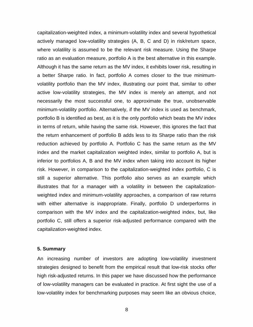
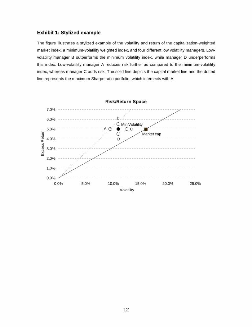
In order to illustrate how different ways of benchmarking can lead to

different conclusions regarding the performance of low-volatility strategies, we

consider the stylized example shown in Exhibit 1. The figure depicts the

that turnover constraints are highly effective at reducing turnover without significantly affecting the long-term risk and return characteristics of the strategy. However, this occurs at the expense of introducing path-dependence. Moreover, as turnover constraints have such a large impact on portfolio composition, the effect on return in the short run is not necessarily negligible.

8

capitalization-weighted index, a minimum-volatility index and several hypothetical

actively managed low-volatility strategies (A, B, C and D) in risk/return space,

where volatility is assumed to be the relevant risk measure. Using the Sharpe

ratio as an evaluation measure, portfolio A is the best alternative in this example.

Although it has the same return as the MV index, it exhibits lower risk, resulting in

a better Sharpe ratio. In fact, portfolio A comes closer to the true minimum-

volatility portfolio than the MV index, illustrating our point that, similar to other

active low-volatility strategies, the MV index is merely an attempt, and not

necessarily the most successful one, to approximate the true, unobservable

minimum-volatility portfolio. Alternatively, if the MV index is used as benchmark,

portfolio B is identified as best, as it is the only portfolio which beats the MV index

in terms of return, while having the same risk. However, this ignores the fact that

the return enhancement of portfolio B adds less to its Sharpe ratio than the risk

reduction achieved by portfolio A. Portfolio C has the same return as the MV

index and the market capitalization weighted index, similar to portfolio A, but is

inferior to portfolios A, B and the MV index when taking into account its higher

risk. However, in comparison to the capitalization-weighted index portfolio, C is

still a superior alternative. This portfolio also serves as an example which

illustrates that for a manager with a volatility in between the capitalization-

weighted index and minimum-volatility approaches, a comparison of raw returns

with either alternative is inappropriate. Finally, portfolio D underperforms in

comparison with the MV index and the capitalization-weighted index, but, like

portfolio C, still offers a superior risk-adjusted performance compared with the

capitalization-weighted index.

5. Summary

An increasing number of investors are adopting low-volatility investment

strategies designed to benefit from the empirical result that low-risk stocks offer

high risk-adjusted returns. In this paper we have discussed how the performance

of low-volatility managers can be evaluated in practice. At first sight the use of a

low-volatility index for benchmarking purposes may seem like an obvious choice,

9

but this approach turns out to be problematic upon closer examination. We first

argued that the unique minimum-variance portfolio from Markowitz’ portfolio

theory is not a useful alternative, because of the fact that it is not observable in

practice. By using predictions of future risk, typically derived from past data, it is

possible to create practical approximations of the theoretical minimum-volatility

portfolio. However, the literature indicates that various approaches are equally

effective, reducing volatility by up to one-third, which implies that it is quite

arbitrary to elevate the status of one of these approaches to benchmark for all

low-volatility approaches.

As an example we discussed the recently introduced MSCI Minimum

Volatility index series, arguing that, rather than being a passive benchmark

alternative for active low-volatility managers, these indices are essentially active

low-volatility investment strategies themselves. First, because the literature

shows that a more simple and transparent quantile portfolio approach is at least

as effective at reducing volatility as the mean/variance optimization approach

used by the MSCI MV indices. Second, because the index construction

methodology relies on a large number of subjective assumptions. And, third,

because of the path-dependent nature of the MSCI MV indices.

Still, in certain cases, it can make sense to evaluate the performance of a

low-volatility manager against a minimum-volatility index such as those of MSCI.

A more robust and generally applicable alternative, however, is to simply

benchmark low-volatility strategies against the capitalization-weighted market

portfolio, using risk-adjusted performance metrics such as Sharpe ratio or

Jensen’s alpha. This approach also recognizes that, at the end of the day, low-

volatility investing is not primarily aimed at beating a certain low-volatility index,

but at establishing a risk/return profile superior to a passive investment in the

capitalization-weighted market index.

References

Arnott, R.D., Hsu, J., and Moore, P. (2005), Fundamental Indexation, Financial

Analysts’ Journal, Vol. 61, No. 2, pp. 83-99.

10

Baker, M.P., Bradley, B., and Wurgler, J.A. (2010), Benchmarks as Limits to

Arbitrage: Understanding the Low Volatility Anomaly, SSRN working paper

no.1585031.

Black, F., Jensen, M.C. and Scholes, M., (1972), The Capital Asset Pricing

Model: Some Empirical Tests, Studies in the Theory of Capital Markets,

Praeger.

Black, F. (1993), Beta and Return: Announcements of the ‘Death of Beta’ Seem

Premature, Journal of Portfolio Management, Vol. 20, No. 1, pp. 8-18.

Blitz, D.C., and van Vliet, P. (2007), The Volatility Effect: Lower Risk Without

Lower Return, Journal of Portfolio Management, Vol. 34, No. 1, pp. 102-

113.

Choueifaty, Y., and Coignard, Y. (2008), Toward Maximum Diversification,

Journal of Portfolio Management, Vol. 35, No. 1, pp. 40-51.

Clarke, R., de Silva, H., and Thorley, S. (2006), Minimum-Variance Portfolios in

the US Equity Market, Journal of Portfolio Management, Vol. 33, No. 1, pp.

10-24.

Clarke, R., de Silva, H., and Thorley, S. (2010), Know Your VMS Exposure,

Journal of Portfolio Management, Vol. 36, No. 2, pp. 52-59.

Falkenstein, E.G. (1994), Mutual Funds, Idiosyncratic Variance, and Asset

Returns, PhD thesis, Northwestern University.

Fama, E.F. and French, K.R., The Cross-Section of Expected Stock Returns,

Journal of Finance, 47 (1992), pp. 427-465.

Fama, E.F. and MacBeth, J.D. (1973), Risk, Return and Equilibrium: Empirical

Tests, Journal of Political Economy, Vol. 71, pp. 43-66.

Haugen, R.A., and Baker, N.L. (1991), The Efficient Market Inefficiency of

Capitalization-Weighted Stock Portfolios, Journal of Portfolio Management,

Vol. 17, No. 3, pp. 35-40.

Maillard, S., Roncalli, T., and Teiletche, J. (2010), The Properties of Equally

Weighted Risk Contribution Portfolios, Journal of Portfolio Management,

Vol. 36, No. 4, pp. 60-70.

11

Markowitz, H. (1952), Portfolio Selection, Journal of Finance, Vol. 7, No. 1, pp.

77-91.

12

Exhibit 1: Stylized example

The figure illustrates a stylized example of the volatility and return of the capitalization-weighted

market index, a minimum-volatility weighted index, and four different low volatility managers. Low-

volatility manager B outperforms the minimum volatility index, while manager D underperforms

this index. Low-volatility manager A reduces risk further as compared to the minimum-volatility

index, whereas manager C adds risk. The solid line depicts the capital market line and the dotted

line represents the maximum Sharpe ratio portfolio, which intersects with A.

Risk/Return Space

CMarket cap

Min Volatility

B

A

D

0.0%

1.0%

2.0%

3.0%

4.0%

5.0%

6.0%

7.0%

0.0% 5.0% 10.0% 15.0% 20.0% 25.0%

Volatility

Exc

ess

Ret

urn