benchmarking of data mining techniques as applied to power
TRANSCRIPT

IT 13 061
Examensarbete 30 hpSeptember 2013
Benchmarking of Data Mining Techniques as Applied to Power System Analysis
Can ANIL
Institutionen för informationsteknologiDepartment of Information Technology

Teknisk- naturvetenskaplig fakultet UTH-enheten Besöksadress: Ångströmlaboratoriet Lägerhyddsvägen 1 Hus 4, Plan 0 Postadress: Box 536 751 21 Uppsala Telefon: 018 – 471 30 03 Telefax: 018 – 471 30 00 Hemsida: http://www.teknat.uu.se/student
Abstract
Benchmarking of Data Mining Techniques as Appliedto Power System Analysis
Can ANIL
The field of electric power systems is currently facing explosive growth in the amountof data. Since extracting useful information from this enormous amount of data ishighly complex, costly, and time consuming, data mining can play a key role. Inparticular, the standard data mining algorithms for the analysis of huge data volumescan be parallelized for faster processing. This thesis focuses on benchmarking ofparallel processing platforms; it employs data parallelization using Apache Hadoopcluster (MapReduce paradigm) and shared-memory parallelization using multi-coreson a single machine. As a starting point, we conduct real-time experiments in orderto evaluate the efficacy of these two parallel processing platforms in terms ofperformance, resource usage (Memory), efficiency (including speed-up), accuracy, andscalability. The end result shows that the data mining methods can indeed beimplemented as efficient parallel processes, and can be used to obtain useful resultsfrom huge amount of data in a case study scenario. Overall, we establish thatparallelization using Apache Hadoop cluster is a promising model for scalableperformance compared with the alternative suitable parallelization using multi-coreson a single machine.
Tryckt av: Reprocentralen ITCIT 13 061Examinator: Ivan ChristoffÄmnesgranskare: Tore RischHandledare: Moustafa Chenine


Page 1 / 75
Acknowledgements
This piece of work was conducted at KTH (Royal Institute of Technology) within the framework of
the EU EP7 iTesla Project in Stockholm. First and foremost, I would like to give special thanks to
my supervisor, Moustafa Chenine, for his patience, advice and constructive comments throughout
the development of this thesis. I would also like to thank Miftah Karim for being a valuable source
of ideas and guidance during the development of this thesis. I would like to express my gratitude to
Tore Risch., my reviewer at Uppsala University, who reviewed my work and shared his worthwhile
opinions; and also to Ivan Christoff, my examiner at Uppsala University, for his invaluable
guidance leading to the completion of this work. Furthermore, my warmhearted thanks go to my
adored family, and – last but not least – my warm thanks go to Melisa Bergström for her invaluable
support.

Page 2 / 75

Page 3 / 75
Contents
1. Introduction ................................................................................................................................... 8
1.1. Problem Statement ............................................................................................................... 8 1.2. Aim and Objective ............................................................................................................... 9 1.3. Delimitations ........................................................................................................................ 9 1.4. Thesis Structure.................................................................................................................. 10
2. Context of Study .......................................................................................................................... 11
2.1. The Electric Power System ................................................................................................ 11 2.2. Data Mining and Knowledge Discovery ............................................................................ 11 2.3. Statistical Correlation ......................................................................................................... 13
2.4. R (programming language) ................................................................................................ 13 2.5. Parallelization..................................................................................................................... 13
3. Related Works ............................................................................................................................. 21
4. Methodology of Study ................................................................................................................. 23 4.1. Method ............................................................................................................................... 23 4.2. Functions ............................................................................................................................ 25
4.3. Case Study.......................................................................................................................... 28
5. Implementation of the Study ..................................................................................................... 31 5.1. Set-up and Configuration ................................................................................................... 31 5.2. Data Selection and Pre-processing ..................................................................................... 33 5.3. Implementation of the Standalone Modules ...................................................................... 34
5.4. Implementation of the Case Study ..................................................................................... 44
6. Evaluation of the Study .............................................................................................................. 46 6.1. Evaluation of the Standalone Modules .............................................................................. 46 6.2. Case Study Evaluation ....................................................................................................... 56
7. Conclusion and Future Work ..................................................................................................... 64
References ......................................................................................................................................... 66
Appendix ........................................................................................................................................... 69 A. Standalone Modules ...................................................................................................................... 69 B. Case Study ..................................................................................................................................... 73

Page 4 / 75

Page 5 / 75
List of Figures
Figure 1: The KDD Process, Step-by-Step ....................................................................................... 12 Figure 2: Map Reduce Example [2] .................................................................................................. 18 Figure 3: R and Hadoop Integration for Hadoop Streaming [2] ....................................................... 19
Figure 4: R and Hadoop Integration for RHadoop [2] ...................................................................... 20 Figure 5: The Phases of Work .......................................................................................................... 23 Figure 6: Development Work-Flow .................................................................................................. 24 Figure 7: Example of K-Nearest Neighbors Algorithms [22] .......................................................... 26
Figure 8: Example of K-means Clustering Algorithms [21] ............................................................ 27 Figure 9: Case Study Scenario Action Flow ..................................................................................... 30 Figure 10: The High-Level Architecture of Apache Hadoop Cluster ............................................... 32
Figure 11: View of Processes After a fork() System Call ................................................................ 36 Figure 12: Flow Chart of Parallel Pearson's Linear Correlation Coefficient Algorithm Based on
MapReduce ........................................................................................................................................ 36 Figure 13: Flow Chart of Parallel kNN Algorithm Based on MapReduce ....................................... 39
Figure 14: Flow Chart of Parallel K-means Algorithm Based on MapReduce ................................ 42 Figure 15: Performance for Stand-alone Modules…..…….... .......................................................... 47
Figure 16: Memory Usage for Stand-alone Modules…………….. ................................................. 49 Figure 17: Accuracy for Stand-alone Modules ................................................................................. 50 Figure 18: Speed-up for Statistical Module on Platform-2 and -3 .................................................... 51
Figure 19: Speed-up for Classification Module on Platform-2 and -3 ............................................. 52 Figure 20: Speed-up for Clustering Module on Platform-2 and -3 ................................................... 52
Figure 21: Efficiency for Statistical Module on Platform-2 and -3 .................................................. 53 Figure 22: Efficiency for Classification Module on Platform-2 and -3 ............................................ 54
Figure 23: Efficiency for Clustering Module on Platform-2 and -3 ................................................. 55 Figure 24: Scale-up for Stand-alone Modules .................................................................................. 55 Figure 25: Comparison of Elapsed Time Spent by Different Platforms for the Data Mining
Processes ............................................................................................................................................ 57
Figure 26: Comparison of Memory Consumption by Different Platforms for the Data Mining
Processes ............................................................................................................................................ 59 Figure 27: Comparison of Accuracy by Different Platforms for Data Mining Processes ............... 59
Figure 28: Speed-up for Data Mining Processes on Platform-2 and -3 ............................................ 61 Figure 29: Efficiency for Data Mining Processes on Platform-2 and -3 .......................................... 61 Figure 30: Scale-up for Data Mining Processes on Platform-2 and -3 ............................................. 62 Figure 31: Prediction of Production Clusters by Cart Decision Tree ............................................... 63
Figure 32: Pearson’s Linear Correlation Coefficient Matrix for Selected Nodes ............................ 70 Figure 33: Pearson’s Linear Correlation Coefficient Scatter Plot Matrix with Regression Analysis
............................................................................................................................................................ 71 Figure 34: kNN result for node A.OTHP3........................................................................................ 72 Figure 35: Pearson’s Linear Correlation Coefficient Values for threshold between - 0.3 and + 0.3
............................................................................................................................................................ 74 Figure 36: Classification Module (kNN classes) Result for Node .OTHP3 ..................................... 75

Page 6 / 75
List of Tables
Table 1: Hardware and Software Information .................................................................................. 32 Table 2: R Packages .......................................................................................................................... 34 Table 3: Average Elapsed Time Spends For Standalone Modules ................................................... 47
Table 4: Memory Consumption for Standalone Modules ................................................................. 49 Table 5: Average Elapsed Time Spent for data mining processes .................................................... 57 Table 6: Memory Consumption for Data Mining Processes ............................................................. 58 Table 7: Pearson’s Linear Correlation Coefficient Values for Selected Nodes ................................ 69

Page 7 / 75

Page 8 / 75
Chapter 1
Introduction
In the last decade, the ongoing rapid growth of modern computational technology has created an
astounding flow of data. As with other industries, the power system field is facing an explosive
growth of data [5], and the development of the electric power industry has resulted in more and
more real-time data being stored in databases. Besides the data from simulations, traditional remote
field devices such as Remote Terminal Units (RTU); a great contribution to this explosive data is
foreseen to originate from new measurement devices such as Phasor Measurement Units (PMUs)
which would be utilized in Wide Area Monitoring and Control systems(WAMC) [5, 40].
Processing and interpreting this huge volume of data is extremely complex, costly and time
consuming [6]. Data mining techniques [7, 40] may be used to extract useful information (i.e.
knowledge) from the huge amounts of data; such as the correlation between power generation and
consumption.
When properly trained up, pattern recognition algorithms in data mining can detect deviation
from the regular data, which may be useful for triggering alarms and messages (classification) that
provide important information to the operator. The mining and off-line analysis of historical data
can provide knowledge that can be subsequently implemented online [8]. This knowledge might be
related to fault analysis, energy consumption, analysis of distributed generation, or load pattern.
Knowledge Discovery in Databases (KDD) aims at extracting useful knowledge from data
[9]. It is a process comprising several steps – selection of target data, data pre-processing, data
transformation, data mining, and evaluation of patterns [9] – and it relies on databases management,
machine learning and statistics. Knowledge discovery and machine learning based on pattern
recognition can provide relevant knowledge to support power systems planning and operation.
1.1. Problem Statement
The problem is that processing enormous amount of data using data mining techniques, while a
good approach, could be time-consuming and slow [6]. One solution would be to apply parallel
processing techniques to data mining, therefore this thesis focuses on:
How data mining algorithms can be parallelized.
Benchmarking of parallel data mining algorithms

Page 9 / 75
Testing those parallel data mining algorithms in a case study scenario (trialed in a case study
scenario).
1.2. Aim and Objective
The main aim and objective of this thesis is to implement data mining algorithms on parallel
platforms and to evaluate them in terms of which parallel platform is the most efficient for
performing data mining processes in the shortest amount of time. The gathered data are subjected to
data mining processing on different parallel platforms with the aim of benchmarking (comparing)
the parallel processing of data mining algorithms as applied to the power system data.
The workflow is as follows:
Devise data mining techniques and methods for implementing them on parallel platforms.
Implement the data mining functions for parallel platforms as standalone modules.
Reuse the standalone modules concurrently in the Case Study, to collect results.
Evaluate the outcomes.
1.3. Delimitations
The scope of this thesis is the benchmarking of sequential and parallel implementations of data
mining algorithms; this benchmarking being conducted on performance, resource usage (CPU and
Memory), efficiency (including speed-up), accuracy and scalability.
Implementation of the decision-tree algorithm as a parallel process is excluded from the
scope of thesis due to time limitations and the complexity of transforming the decision tree
sequential algorithm to the MapReduce programming paradigm.
In this study, the size of the test beds that are used to conduct the analysis of parallel
processes are limited by the use of one single machine with four cores (for parallel computing) and
a small size of Apache Hadoop cluster size—four nodes (for distributed computing).
The study includes only one case study due to there being no feasible and implementable
real use case scenarios for analyzing power systems.

Page 10 / 75
1.4. Thesis Structure
Following this introductory chapter (chapter 1) the thesis continuous with chapter 2 which describes
the general context of this study. In the subsequent chapters 3, 4, 5 and 6, I explain in details my
approach to applying data mining techniques to power systems. Therefore, chapter 3 presents the
related works, chapter 4 presents our methodology, chapter 5 introduces the reader to the
implementation details of the work, and chapter 6 provides an evaluation details of the work. The
final chapter presents conclusions and ideas for taking this work further are given in the final
chapter.

Page 11 / 75
Chapter 2
2. Context of Study
This chapter presents the background information that will help set the scene and give a better
understanding of the subject matter for this study.
2.1. The Electric Power System
Electric power systems are critical infrastructures for modern society [19, 34, and 35]. They span
huge geographical areas, and comprise thousands of measurement and monitoring systems
continuously collecting various data such as voltage and current, power lows, line temperatures,
plus data relating to the stating of devices.
The increased utilization of information and communication technologies make available a
wealth of data which can be used to gain a deeper understanding of the dynamics of the process as
well as an opportunity to use data in online decision support.
For example, systems like Wide Area Monitoring and Control (WAMC) continuously
collect data at a high sampling rate (e.g. 50 samples per second),where each sample can be several
measurements [34, 35].
2.2. Data Mining and Knowledge Discovery
Knowledge Discovery in Databases (KDD) is the process of discovering useful knowledge from a
huge amount of data [5, 6, and 13]. This means preparing and selecting the data to be mined,
cleaning the data, incorporating prior knowledge, and deriving solutions from the observed results.
While KDD is commonly used to refer to the overall process of discovering useful
knowledge from data, data mining refers to the particular step in this process which involves the
application of specific algorithms for extracting patterns from data. Data mining is defined as “the
nontrivial extraction of implicit, previously unknown, and potentially useful information from
data” [16]. Thus the overall aim of the data mining process is to derive useful information /
knowledge from raw data, by a process of transformation into a structure that is suitable for further
processing or direct application [5, 6, and 13].

Page 12 / 75
Figure 1: The KDD Process, Step-by-Step
2.2.1 Data Mining Tasks
This section presents information about the various data mining methods.
2.2.1.1. Predictive:
This is a data mining task that uses certain variables to predict unknown or future values of other
variables. It is achieved by subjecting a huge amount of data to a training regime known as
supervised learning, whereby estimated values are compared with known results [13].
Classification: Given a set of predefined categorical classes, this task attempts to determine which
of these classes a specific data item belongs to. Some commonly used algorithms in classification
are C4.5, K-Nearest Neighbors (KNN) and Naï ve Bayes [9].
Regression: Uses existing values to forecast what other values will be. Simply, regression uses
standard statistical techniques such as linear regression. But many real-world problems such as
stock price changes and sales volumes do not lend themselves to prediction via regression, because
they depend on complex interactions of multiple variables. Therefore, some other more complex
techniques such as logistic regression or neural networks may be necessary in order to forecast
future values. The same model types, such as Classification and Regression Trees (CART), can
often be used for both regression and classification; its decision tree algorithm can be used to build
both classification trees (to classify categorical response variables) and regression trees (to forecast
continuous response variables). Neural nets can also be used to create both classification and
regression models.
2.2.1.2. Descriptive:
No training data is used here, and it is sometimes referred to as unsupervised learning because there
is no already-known result to guide the algorithms [9].
Clustering: Involves separating data points into groups according to how “similar” their attributes
are. A commonly used algorithm for clustering is K-means [9].

Page 13 / 75
2.3. Statistical Correlation
Correlation is a statistical technique that tells us whether two variables are related to each other—
either positively or negatively, and to what degree (strength of correlation) [8].
One of the most common methods of computing correlation is Pearson’s linear correlation
coefficient. Pearson's linear coefficient correlation (r) is a numerical value that ranges from + 1.0
to - 1.0, where r > 0 indicates a positive relationship and r < 0 indicates a negative relationship; and
where r = 0 indicates there is no relationship between variables. The closer we get to +1.0 or -1.0,
the stronger the relationship (positive or negative) between the variables [31].
2.4. R (programming language)
R is a GNU project; it is an interpreted programming language which is typically used through a
command line interpreter [33]. R is a highly efficient, extensible, elegant and comprehensive
environment for statistical computing and graphics. The R programming language is used to
develop parallel platforms. One of the important features of R is that it supports user-created R
packages and a variety of file formats (including XML, binary files, .csv) [33].
2.4.1. Drawbacks of R
The most significant limitations of R are that it is single-threaded and memory-bound [20]:
It is single-threaded:
The R language has no explicit constructs for parallelization, such as threads. An out-of-the-box R
installation cannot take advantage of multiple CPUs. Regardless of the number of cores on your
CPU, R will only use one core by default.
It is memory-bound:
Whereas other programming languages read data from files as needed, R requires that your entire
data set fits in memory (RAM) because all computation is carried out in the main memory of the
computer. This is a problem because four gigabytes of memory (for example) will not hold eight
gigabytes of data, no matter what.
2.5. Parallelization
A large amount of computing resource (execution speed) and storage space (memory) is required to
extract useful knowledge from large amounts of data [11]. Parallelization or distributed computing
allows us to speed up computations by using multiple CPUs or CPU cores to run several
computations concurrently. Although parallel and distributed computing are not exactly the same,
they serve the same fundamental purpose of dividing large problems into smaller problems that can
be solved concurrently.
The following factors are important in parallelization:

Page 14 / 75
Execution Speed
Execution speed can be improved by parallelizing operations either a) within a processor using
pipelining or multiple arithmetic logic units (ALUs), or b) between processors with each
processor working on a different part of the problem in parallel [11].
Memory
The memory capacity of several machines can be utilized for parallel or distributed processing,
to overcome the problem of no single machine having sufficient memory for processing of large
data sets [11].
Concurrency
A single computing resource can do only one thing at a time whereas multiple computing
resources can do many things simultaneously.
There are broadly two taxonomies of parallel or distributed computing, depending on the
computation model (task / data parallelization) and communication model (message passing /
shared memory) that is employed [11, 12]. Task parallelization splits computation tasks into distinct
subtasks (different computation programs) that are assigned to different computing units, whereas
data parallelization (master / slave architecture) involves all computing units running the same
program but on different data. The message passing model involves messages being exchanged
between different tasks (or computing units), whereas the shared memory model involves
communication by reading / writing to a shared memory location.
This thesis focuses on the data parallelization using Apache Hadoop cluster (master-slave
architecture and MapReduce paradigm), and shared-memory parallelization using multi-cores on a
single machine.
2.5.1. Parallel Computing with R
The R programming language is a sequential language. That is, program instructions are executed
one-at-a-time in strict sequence from the top to the bottom of the program (subject control of flow
operations such as loops and conditions). In contrast—parallel computing allows different program
instructions to be executed simultaneously; or the same program instructions to be simultaneously
on different data.
In recent years, a great number of studies [39] have focused on the problem of extensive
analysis, some researchers in the open source R community have developed high computing
packages that provide R scripts able to run on clusters or multi-core platforms. According to [39],
there are two general schemes of parallel computing R packages; “building blocks” and “task
farm”. The first scheme offers basic parallel building blocks such that a parallel implementation of
an algorithm can be developed, whereas latter is where a 'master' process (node) feeds a pool of
'slave' processes (nodes) with subtasks. Typical uses are performing the same algorithm on each
slave node with different data; or perform different analysis on the same data. Thus, there are
several ways to parallelize the sequential R language with high-performance computing R packages
Page 15 / 75
[20, 39]. One other option could be to start an R session on each of several computers, and
effectively run the same program on each of them. Other possibility could be to use Apache Hadoop
framework as distributed computing [20].
In the following we describe in detail master-slave architecture (which is analogous to “task
farm” parallelization of taxonomy) and shared-memory parallelization (which is analogous to
“building blocks” parallelization of taxonomy).
2.5.1.1. Shared Memory Parallelization (Parallel Computing)
In this parallelization, tasks share a same address space to read and write (asynchronously) [14].
Multi-core architecture is defined to a single processor packages that has two or more processor
execution cores [24]. In a multi-core microprocessor, each core solely performs optimizations such
as pipelining and multithreading. Further, in a multi-core microprocessor, with divide-and-conquer
strategy multi-core architecture carries out more work in a given clock cycle [24].
Since all threads run on the same computer there is no need for network communication in a
multi-core parallelization. On the other hand, as every thread has access to all objects on the heap
there is a extensive need for concurrency control to not to violate data integrity as parallelization of
the program[11]. A great way to provide concurrency is using locks [11]. Compared to master-slave
parallelization, constructing shared-memory parallelization reduces the overhead of communicating
through a network. Shared memory parallelization with R is currently limited to a small amount of
parallelized functions [39]. A key advantage of shared-memory parallelization is data sharing
among the tasks are fast and uniform [14]. On the other hand, the main drawback is the lack of
scalability between memory and CPUs. Adding more CPUs could dramatically increase traffic on
the path between shared-memory and CPU [14].
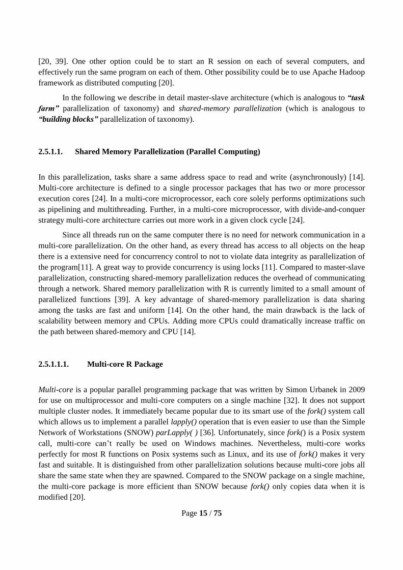
2.5.1.1.1. Multi-core R Package
Multi-core is a popular parallel programming package that was written by Simon Urbanek in 2009
for use on multiprocessor and multi-core computers on a single machine [32]. It does not support
multiple cluster nodes. It immediately became popular due to its smart use of the fork() system call
which allows us to implement a parallel lapply() operation that is even easier to use than the Simple
Network of Workstations (SNOW) parLapply( ) [36]. Unfortunately, since fork() is a Posix system
call, multi-core can’t really be used on Windows machines. Nevertheless, multi-core works
perfectly for most R functions on Posix systems such as Linux, and its use of fork() makes it very
fast and suitable. It is distinguished from other parallelization solutions because multi-core jobs all
share the same state when they are spawned. Compared to the SNOW package on a single machine,
the multi-core package is more efficient than SNOW because fork() only copies data when it is
modified [20].

Page 16 / 75
Advantages [32]:
Able to load-balance with multi-core.
Able to set the number of cores.
Fast.
Overcomes the single-threaded nature of R.
Easy to install and use.
Disadvantages [32]:
Does not work in Microsoft Windows.
Need high memory hardware.
2.5.1.2. Master-slave Parallelization (Distributed Computing)
In this parallelization , a large data set is usually split into smaller pieces and distributed through the
cluster by the main computation node—the master node, a subtask for its subsets are solved by
other computing nodes—the slave nodes. The slave nodes do not communicate each other, they
responsible to execute the task and return the result to master, while the master node is responsible
to start the slave nodes. This type parallelization is very suitable for clusters or supercomputers and
MapReduce paradigm [2, 3, and 40]. Since each slave node has own local memory space, this type
of architecture can be defined as distributed shared memory as well [14]. While the load-balancing
of the computing nodes is well handled, the parallelization scales linearly with the number of
computing nodes [11]. Another advantage for this parallelization is each computing node can easily
access its own memory without any interference and the overhead [14].
2.5.1.2.1. Apache Hadoop Project
Apache Hadoop is a first class open-source project hosted by Apache Software Foundation [2, 3]. It
is a framework that makes it possible to process huge data sets through clusters of computers using
basic programming models. Apache Hadoop does not rely on hardware in order to provide high-
availability; the software library is designed so that it can detect and handle failures at the
application layer [2, 4]. The storage and computational capabilities are designed so that it scales up
from a single server to thousands of machines [2], with each machine providing its own storage and
computation.
The Apache Hadoop framework comprises eleven sub-projects that provide distributed
computing and computational capabilities. Although Hadoop MapReduce and Hadoop Distributed
File Systems (HDFS) are known and used widely [3], other projects provide supplementary
functions.
Page 17 / 75
Hadoop is a distributed master-slave architecture which has two main components: HDFS for
storage and MapReduce for computational capabilities. One of the biggest benefits of the Hadoop
ecosystem is that it can be integrated with any programming language, such as R or Python [2, 3].
A- Hadoop Distributed File Systems (HDFS)
Apache Hadoop comes with a distributed file system called HDFS, which stands for Hadoop
Distributed File System. It is ideal for storing large amounts of data (terabytes and petabytes) [2].
HDFS provides seamless access to files that are distributed across nodes in different clusters, and
those virtual files can be accessed by the MapReduce programming model in a streaming fashion.
HDFS is fault-tolerant and it provides high-throughput access to large data sets [1, 2].
HDFS is similar to other distributed file systems, except for the write-once-read-many
concurrency model [1] that simplifies data coherency and enables high-throughput access. Some of
the notable HDFS features are [1, 2]:
Detection and quick automatic recovery from faults.
Data access via MapReduce streaming.
Simple and robust coherency model.
Enable portability between very different commodity operating systems and hardware.
Scalability to store and process large amounts of data.
Distribution of data and logic to nodes where data is located, for efficient parallel
processing.
Reliability, resulting from maintaining multiple copies of data and automatically
redeploying processing logic in the event of failures
B- Hadoop Map-Reduce
MapReduce was popularized in a Google paper, “MapReduce: Simplified Data Processing on
Large Clusters” [1] by Jeffrey Dean and Sanjay Ghemawat. In the time since Google built their
own implementation to churn web content, MapReduce has been applied to other problems [1].
MapReduce is a data parallelization programming model—the dataset is split into
independent subsets and distributed, then the same instructions are applied to each subset in
concurrently [42] , for processing and generating huge amounts of datasets [2, 3]. It is inspired by
functional languages and is aimed at data-intensive computations, such as Google’s original use to
regenerate the index of the World Wide Web [31].
The MapReduce model outlines a way to perform work across a cluster of inexpensive
commodity machines. Simply put, there are two phases: Map and Reduce. Although the input to
MapReduce can vary according to application, the output from MapReduce is always a set of (key,
value) pairs. The programmer writes two functions, the Map function and the Reduce function as
follows:
The Map function is applied to the input data, and produces a list of intermediate (key,
value) pairs that can vary according to application, algorithm, and programmer.

Page 18 / 75
The Reduce function is then applied to the list of intermediate values (map function outputs)
that have the same key. Typically this is some kind of convergence or merging operation
which produces (key, value) pairs as output.
A key benefit of the MapReduce programming model is that the programmer does not need to
deal with the complicated code parallelization, and can therefore focus on the required computation
A simplified version of a MapReduce job proceeds as follows:
Map Phase
1. Each cluster node takes a piece of the initial huge amount of data and runs a Map task on each
record (item) of input. You supply the code for the Map task.
2. All of the Map tasks run in parallel, creating a key/value pair for each record. The key identifies
the item’s fragment for the Reduce operation. The value can be the record itself or some derivation
of it.
The Shuffle (Hadoop does this phase automatically)
1. At the end of the Map phase, the machines all pool their results. Every key/value pair is assigned
to a fragment, based on the key. (Hadoop does this automatically)
Reduce Phase
1. The cluster machines then switch roles and run the Reduce task on each pile. You supply the
code for the Reduce task, which gets the entire pile – that is, all of the key/value pairs for a given
key – at once.
2. The Reduce task typically (but not necessarily) emits some output for each pile.
Figure 2 provides a visual representation of a MapReduce flow as an example. Let's consider
an input in which each line is a record of the format (letter and number), and the aim is to find the
maximum value of number for each letter. Step (1) describes the raw input. In Step (2), the
MapReduce system provides each record’s line number and content to the Map process, which
splits the record into a key (letter) and value (number). The Shuffle step gathers all of the values for
each letter into a common bucket, and feeds each bucket to the Reduce step. In turn, the Reduce
step plucks out the maximum value from the bucket. The output is a set of (letter, maximum
number) pairs.
Figure 2: Map Reduce Example [2]

Page 19 / 75
2.5.1.2.2. Integration with R and Apache Hadoop Project
A. R and Apache Hadoop Streaming
With Hadoop Streaming, the Map and Reduce functions can be written in any programming
language or script that allows the reading of data from standard input and the writing of data to
standard output. R supports this feature, so it can easily be used with Apache Hadoop framework; as
illustrated in Figure 3, R and Hadoop Streaming can be used to process data in a MapReduce job
just like the regular MapReduce.
Using Apache Hadoop framework overcomes the single-threaded and memory boundary
limitations of R. Another big advantage is that Hadoop provides scalability. The only drawback is
that the implementation breaks up a single logical process into multiple scripts and steps due to
MapReduce programming framework.
Figure 3: R and Hadoop Integration for Hadoop Streaming [2]
B. RHADOOP
There is another way to integrate R and Apache Hadoop framework—using the RHadoop open
source project created by Revolution Analytics. RHadoop allows users to use MapReduce
interactions directly from within R without touching Hadoop so much.
RHadoop consists of two components:
Rmr: This R package allows an R programmer to perform statistical analysis via MapReduce on a
Hadoop cluster. The rmr package uses Hadoop streaming, and one of the most important features of
rmr is that it makes the R client-side environment available to the Map and Reduce functions of R
that are executed in MapReduce. The integration between R and Hadoop via RHadoop as depicted
in Figure 4.

Page 20 / 75
Figure 4: R and Hadoop Integration for RHadoop [2]
Rhdfs: This R package provides basic connectivity to the Hadoop Distributed File System (HDFS),
enabling programmers to browse, read, write, and modify HDFS files.

Page 21 / 75
Chapter 3
3. Related Works
In recent years, a great number of studies [37] have investigated parallel data mining methods, with
a view to making them faster via different implementations. Most research on parallel data mining
[38] has focused on the efficient parallelization of distributed computing, but – because almost
every computer has multiple cores nowadays [11] – shared memory parallelization (implicit
parallelization) has become popular. Parallel data mining algorithms are proposed for symmetric
multiprocessing (SMP) in [40, 42]. McKmeans [11] discusses thread programming, whereby a
sequential program is split into several tasks which are then processed as threads. The paper
introduces highly efficient multi-core parallelization of k-means; parallelized by simultaneously
calculating by the minimum distance partition and the centroid update. The results are compared to
sequential K-means R and McKmeans parallel implementation (similar way of parallel
implementation of k-means clustering in implicitly) in terms of runtime performance for various
datasets. In the other paper [42], the split data points are handled in agents rather than threads.
Different parallel k-means algorithms are compared based on runtime performance, these
algorithms being: paraKmeans [41], sequential R and clojure [42]. Performance characterization of
individual data mining algorithms has been documented in [43], a paper which focuses on the CPU
performance and cache (memory) behaviors of data mining applications such as association rule
mining, clustering, and classification. Ying [44] presented MineBench as a benchmarking suite
which comprises data mining application, plus evaluation of classification, clustering and ARM
categories of data mining applications with implemented using C/C++. They show that the
performance is impacted by synchronization overheads and I/O Time rather than by OS overheads
and the overall performance of the data mining applications. Most of the parallel data mining
algorithms for classification and clustering based on MapReduce [23, 25, and 27] are implemented
in similar way to our implementations in this thesis, although the different tools are used—such as
Weka [45].
Since R is a very widely used statistical tool, many studies have been done to adapt it for
parallelization platforms; thus many R parallel packages have been developed—such as RMPI,
SNOW, and SPRINT [36]. Another work in this area is introduced and evaluated in [39]:
parallelization for Pearson correlation. This introduced the simple parallel R interface (SPRINT)
framework for HPC (High Performance Computing) systems. This study is very similar to our study
in terms of the parallelization method, since we have used another common parallel (High
Performance Computing) R package; the multi-core R package. Many of the other R parallel
packages could be investigated in depth as a future study.

Page 22 / 75
Most of the previous work either focuses on specific data mining methods such as
classification, clustering and association rules, or is limited to one particular programming language
such as Java, or C. Examples include: Yanyan et al [23], Vineeth et al [43], and Ying et al [44].
Most of these compare the performance of data mining methods only in terms of runtime and speed
up [23, 25], whereas in our thesis, we provide a comprehensive study of parallel data mining
algorithms benchmarked with five different metrics. In addition to runtime and speedup, we also
investigate scalability, efficiency, resource usage (Memory) and accuracy metrics.
To our knowledge there exists no evaluation of data mining algorithms based on our
performance metrics—scalability, efficiency, and resource usage (Memory)—when implemented
using the R programming language either with distributed Hadoop MapReduce framework or multi-
core R parallel package prior to this work.

Page 23 / 75
Chapter 4
4. Methodology of Study
This chapter presents the phases of work, the functions, and the case study.
4.1. Method
Figure 5 shows the steps that were followed to achieve the desired goals, with these steps being
described in detail in the sections that follow.
Figure 5: The Phases of Work
4.1.1. Literature Review
The literature review was carried out first to understand the parallel programming models and data
mining techniques, and most of the material has been included in chapter 2 as background material.
Since the programming language chosen for the project was R, additional investigation was needed
to discover how tasks could be parallelized in R. The resources for the literature review were
collected from Internet sources including published technical papers.
4.1.2. Design
The design phase of the project began with the selection of data mining algorithms appropriate to
electric power system analysis [13] and to the aims of the thesis; it continued with the selection of
parallelization models. It was decided to use two different parallel models: parallel programming
using multi-cores via R packages, and MapReduce with the Apache Hadoop framework. The
memory-bounded and single-threaded limitations of the R architecture were considered. The
Apache Hadoop framework was selected as the most suitable solution for our kind of data: huge and
stored (like log files—not updated frequently). Other factors in choosing the Apache Hadoop
framework were that it is compatible with all languages, it has distributed file system, provides fault
tolerance [2,24], and imposes no limitations on the data format or size. Hadoop and R could be
integrated with RHadoop [20] and Hadoop Streaming [20], and the R multi-core package was used

Page 24 / 75
in order to facilitate multi-core computing.
4.1.3. Implementation
Since the main aim of the project was to extract useful knowledge from the huge data, prior to the
development phase we created a case study (shown later in Figure 9). Therefore we could divide the
development phase into two sections: standalone modules and case studies. The first statistical
module was implemented in a sequential way, then implemented in a multi-core way, and finally
implemented for Hadoop. Other modules were implemented in similar fashion as shown in Figure
6, and these modules were run concurrently for the case study.
Figure 6: Development Work-Flow
4.1.4. Selection of Metrics
The selection of metrics for this work included:
Performance:
The elapsed execution times of programs were measured, to find out which functions ran fastest on
various platforms.
Memory Consumption:
The memory consumption (in megabytes) was measured, to determine the memory consumption of
the platforms while running functions in practice.
Accuracy:
The purpose of accuracy comparison was to find out the correctness of the platforms' results when
running the parallel (with Hadoop and with multi-core) and sequential models.

Page 25 / 75
Efficiency:
Efficiency tells us how much of the available processing power is being utilized, which we can
measure using the formula:
Efficiency = Speedup / p, where p is the number of cores or nodes [26, 28].
Thus we are calculating Efficiency as the speedup per processor (core or node).
The Speedup itself is measure of how the execution time is improved by parallelization; it
can be expressed as the ratio of the sequential execution time to the parallel execution time as
follows:
Speedup (n) = T (1) / T (n), where n is the number of computing nodes. T(1) is the execution
time of the tasks in series on 1 computing node or core, and T(n) is the execution time of the tasks
in parallel with n computing nodes or cores [26, 28].
Scale Up ( scale vertically):
Scale Up is a measure of how the system and data size can grow as a result of parallelization. It can
be expressed as follows:
Scale up (n) = T (1, D) / T (n, nD) where n is the number of computing nodes or cores, T (1,
D) is the execution time of the tasks on 1 computing node or core with data size of D, and T (n, nD)
is the execution time of the parallel tasks on n computing nodes or cores with data size of n times D
[29].
Simply put, Scale up is defined as the ability of a larger system (n-times larger) to perform a
larger job (n-times larger) in the same time as the original system.
4.1.5. Evaluation
After the metrics were selected, the evaluation was done in two ways: evaluation of the standalone
modules, and then evaluation of the case study (with the standalone modules used concurrently).
4.1.6. Result
In order to achieve the aims of this thesis, the standalone modules were evaluated in terms of their
suitability for parallel data mining, and the case study was brought to a conclusion with a CART
decision tree.
4.2. Functions
This section represents the functions for this work, including:
Pearson's Linear Correlation Coefficient
In order to calculate correlations between node pairs, Pearson’s linear correlation coefficient (r)
function was used. The function is as follows [31]:

Page 26 / 75
Equation 1: Equation for Pearson’s linear correlation coefficient
K-Nearest Neighbor Classification ( kNN )
KNN is a supervised instance-based learning algorithm used for classifying objects based on closest
training examples in the feature space. The kNN algorithm is relatively simple: it classifies an
object according to the majority vote of its neighbors, so that the object is assigned to the class most
common amongst its K nearest neighbors. There is no one-size-fits-all optimal number for the
choice of K, and a good choice is often derived through heuristic approaches such as cross-
validation. Choosing a large value for K could reduce the effect of noise, but it could result in
computation inefficiency and the “blurring” of class boundaries. Hence a small positive integer is
typically chosen for practical implementation, and in a special case where K = 1 (the nearest
neighbor algorithm) the object is simply assigned to the class of its nearest neighbor. The selection
of K-nearest neighbors is based on the distance between two data points in the feature space, with
Euclidean distance usually being used as the distance metric. For every unknown instance, the
distance between the unknown instance and all the instances found in the training set is calculated.
The K instances in the training set that have the nearest distance to the unknown instance are
selected, and the unknown instance will be assigned the class of the dominating neighbors. Figure 7
illustrates the kNN algorithm for a two-class example.
Figure 7: Example of K-Nearest Neighbors Algorithms [22]
The unknown instance (denoted as green circle) should be classified either as a blue square
or a red triangle. If k = 3 (denoted by the inner circle), it is classified as a red triangle because there
are two squares and only one square. If k = 5 (denoted by the outer circle), it is classified as a blue
square because there are now three squares vs. two squares.
Algorithm
A high level summary of the nearest-neighbor algorithm method is shown below. The algorithm
computes the distance (or similarity) between each test example z = (x', y') and all the training
examples (x, y) E D to determine its nearest-neighbor list, Dz. Such computation can be costly if the
number of training examples is large. However, efficient indexing techniques are available to
reduce the number of computations needed to find the nearest neighbors of a test example.

Page 27 / 75
1: Let n be the number of nearest neighbors and D be the set of training examples
2: for each test example z0 (x’, y’) do
3: Compute d (x’, x), is the distance between z and every example of D.
4: Set of k closest training examples to z
5: y’= argmax
v∑ (x i , yi)∈ D z I (v= y i )
6: end for
K-means Clustering
K-means is a method of cluster analysis whereby a set of data points (n) is partitioned into a number
of clusters (k) such that each data point belongs to the cluster with the nearest mean. It is one of the
simplest clustering algorithms, and its aim is to calculate sum-of-squares distances within the
clusters.
Given a set of data points (x1 , x2 , ..., xn ) where each point is a d-dimensional vector,
following the assignment to k centroids (μ1 , μ2 , ..., μk ) we will have k partitions S = {S1 , S2 , ...,
Sk }.
The K-means function can be written as follows:
Equation 2: Equation for K-means Clustering Function
Figure 8: Example of K-means Clustering Algorithms [21]
Step 1: In the Figure 8 (a), K initial “means” are arbitrary selected within the data set. In this
example the cluster number k = 3 so that the first clusters are red, green and blue ones.
Step 2: In the Figure 8 (b), selected K clusters are created based on every observation with the

Page 28 / 75
nearest mean.
Step 3: In the Figure 8 (c), the centroid of each of the k clusters is centered on new mean. Since K-
means is an iterative algorithm, Step 2 and Step 3 are repeated until there is no convergence.
In the Figure 8 (d) is the final result of clusters and its centroids.
Classification and Regression Trees
Classification and Regression Trees (CART) is a nonparametric binary recursive partitioning
procedure that is introduced as an umbrella term for the following types of decision trees:
Classification Trees in which the target variable is categorical. The classification tree is used
to identify the class within which a target variable would likely fall.
Regression Trees in which the target variable is continuous and the regression tree is used to
predict its value. Trees are grown to maximum size without any stopping rule, and then
branches are pruned back split-by-split to the root. The next split to be pruned is the one that
is contributing least to the overall performance of the tree on training data [13].
The CART algorithm comprises as a series of questions, each of which determines what the
next question (if any) will be. The result is a tree structure whose branches end with terminal nodes
that represent the points at which no more questions will be asked (and the deduced solutions can be
found).
4.3. Case Study
Innovative Tools for Electrical System Security within Large Areas (iTesla) is a collaborative R&D
project co-founded by the European Commission with a primarily goal of developing and validating
an open interoperable toolbox for the future operation of the Pan-European grid. The iTesla project
requires a great deal of data mining investigation in order to:
Manage statistical post-treatments of power system simulations.
Chain up data mining modules required for security analysis, and insert data mining features
within the power system work flow.
Feed power system studies and processes with data.
In order to fulfill the data mining demands of the iTesla project, one real-life case scenario (case
study) is used in this thesis.
Page 29 / 75
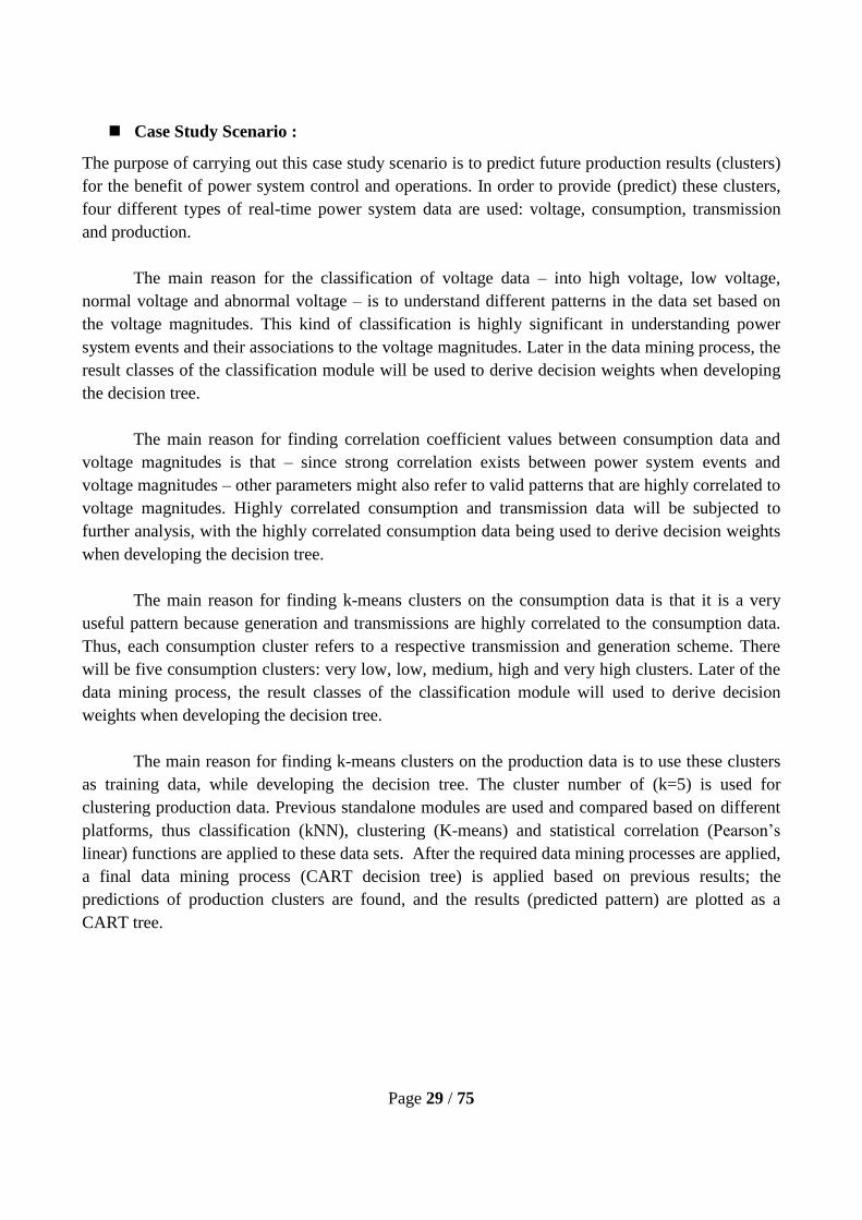
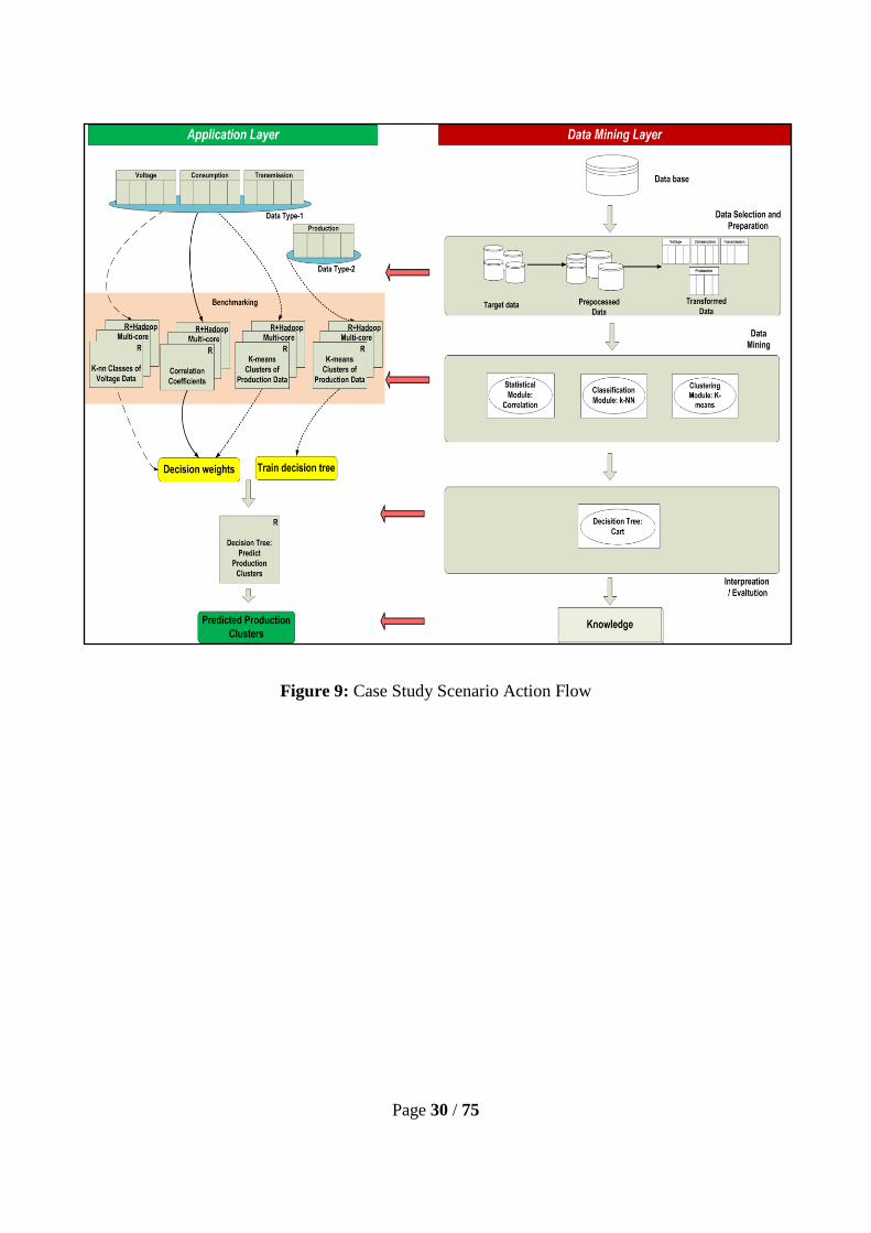
Case Study Scenario :
The purpose of carrying out this case study scenario is to predict future production results (clusters)
for the benefit of power system control and operations. In order to provide (predict) these clusters,
four different types of real-time power system data are used: voltage, consumption, transmission
and production.
The main reason for the classification of voltage data – into high voltage, low voltage,
normal voltage and abnormal voltage – is to understand different patterns in the data set based on
the voltage magnitudes. This kind of classification is highly significant in understanding power
system events and their associations to the voltage magnitudes. Later in the data mining process, the
result classes of the classification module will be used to derive decision weights when developing
the decision tree.
The main reason for finding correlation coefficient values between consumption data and
voltage magnitudes is that – since strong correlation exists between power system events and
voltage magnitudes – other parameters might also refer to valid patterns that are highly correlated to
voltage magnitudes. Highly correlated consumption and transmission data will be subjected to
further analysis, with the highly correlated consumption data being used to derive decision weights
when developing the decision tree.
The main reason for finding k-means clusters on the consumption data is that it is a very
useful pattern because generation and transmissions are highly correlated to the consumption data.
Thus, each consumption cluster refers to a respective transmission and generation scheme. There
will be five consumption clusters: very low, low, medium, high and very high clusters. Later of the
data mining process, the result classes of the classification module will used to derive decision
weights when developing the decision tree.
The main reason for finding k-means clusters on the production data is to use these clusters
as training data, while developing the decision tree. The cluster number of (k=5) is used for
clustering production data. Previous standalone modules are used and compared based on different
platforms, thus classification (kNN), clustering (K-means) and statistical correlation (Pearson’s
linear) functions are applied to these data sets. After the required data mining processes are applied,
a final data mining process (CART decision tree) is applied based on previous results; the
predictions of production clusters are found, and the results (predicted pattern) are plotted as a
CART tree.
Page 30 / 75
Figure 9: Case Study Scenario Action Flow

Page 31 / 75
Chapter 5
5. Implementation of the Study
This implementation chapter comprises four main parts. The first is the setup and configuration of
the programming language, its packages, and Apache Hadoop cluster. The second part is about the
data and its preparation. The third part is about implementation of the algorithms for three chosen
modules and the decision tree function. The fourth and final part is the subsequent running of the
modules concurrently in the context of the use case scenario (case study).
5.1. Set-up and Configuration
The experiment is carried out on three different platforms as follows, with the implementation
language being R and the operating system being Ubuntu Linux in all cases.
For Platform-1 a single machine (machine-1) is used, and only the R language is installed
(for sequential processing).
For Platform-2 a single machine (machine-1) is used, and parallelization is achieved by
combining R with the multi-core package.
For Platform-3, the four machines detailed in
Table 1 is used. These machines are arranged as a Hadoop cluster with machine-1 as a master
and the other machines as slave nodes.
Information’s /
Machines
Machine - 1
(Master)
Machine – 2
(Slave-1)
Machine – 3
(Slave -2)
Machine – 4
(Slave -3)
Processor Intel® Core™ i5-
2410M CPU @
2.30GHz × 4
Intel® Core™ 2
Duo CPU E6750 @
2.66 GHz × 2
Intel® Core™ 2
Duo CPU E4600 @
2.40 GHz × 2
Intel® Core™ 2
Duo CPU E4600 @
2.40 GHz × 2
Memory 3.8 GİB DDR2 1.9 GİB DDR2 1.9 GİB DDR2 1.9 GİB DDR2
Os Type 64-bit 64-bit 64-bit 64-bit
Operating
System
Ubuntu 12.10 Ubuntu 12.10 Ubuntu 12.10 Ubuntu 12.10
R Version 2.15.2 2.15.2 2.15.2 2.15.2

Page 32 / 75
Apache Hadoop
Version
1.0.4 1.0.4 1.0.4 1.0.4
Table 1: Hardware and Software Information
Since Platform-3 will be used for parallel R based on MapReduce, the Apache Hadoop installation
and configuration is done on all four machines. RHadoop is installed on all computing nodes along
with the R language, and the Hadoop cluster architecture is presented in Figure 10.
Figure 10: The High-Level Architecture of Apache Hadoop Cluster

Page 33 / 75
Configuration of Hadoop Clusters:
As depicted in Figure 10, there is one master node and three slave nodes. The following
configurations are necessary in order to set up one machine as the master and the other machines as
slaves. One machine (master) in the cluster is designated as the NameNode and Jobtracker. The
other machines in the cluster act as a “worker nodes” which are simply slave nodes that act as Data
Node and TaskTracker (Figure 10)
5.2. Data Selection and Pre-processing
The implementation begins with the selection of data from the huge database. The datasets were
selected based on the requirements of the case study scenario; therefore four different data sets were
selected:
Voltage Data: The voltage data represents the voltage values between two points, which in
our case are nodes. In power systems, the voltage ranges from low-voltage to ultra-high
voltage [10].
Consumption Data: The consumption data represents the voltage values for the electrical
energy that is used by all the various loads on the power system. In addition, consumption
also includes the energy used to transport and deliver the energy [10].
Transmission Data: The transmission data represents voltage values which are used by the
power system to transport electrical energy efficiently over long distances to the
consumption locations [10].
Production Data: The production data simply represents voltage values that are produced
by the power system [10].
Since the data is gathered in real time and this project is carried out under the umbrella of the
iTesla project, the data sets were handed over to us as a raw data in the .csv file. In order to make
these data sets suitable for data mining purposes, they were subjected to operations such as data
cleaning (including removal of out-of-range values), data merging, and transformation into the
required file format. All of the data selection and pre-processing operations were done sequentially
using by the R language. Listing 1 illustrates an example of the code (for data cleaning) is as
follows:

Page 34 / 75
Listing 1: Source Code for Data Cleaning
5.3. Implementation of the Standalone Modules
This section details the implementation of the algorithms for the three different modules. To begin,
Table 2 lists all of the R packages that are used for the implementation phase.
Title Version Description
multicore 0.1-7 Parallel processing of R code on machines with multiple cores or CPUs.
class 7.3-7 Provides various functions for classification.
rmr2 2.2.0 Allows statistical analysis to be performed via MapReduce on a Hadoop
cluster using the R programming language.
rhdfs 1.05 Provides basic connectivity to the Hadoop Distributed File System (HDFS)
so that R programs can read, write, and modify files.
outliers 0.14 Provided to test for outliers.
corrgram 1.4 Allows us to plot a diagram.
lattice 0.20-15 A powerful and elegant high-level data visualization system.
rbenchmark 1.00 Benchmarking routine for R.
stats 2.15.3 This package contains functions for statistical calculations and random
number generation
utils 1.23.2 Provides various programming utilities.
rpart 4.1-1 A toolkit for regression trees and recursive partitioning.
partykit 0.1-5 A toolkit that allows tree structure regression and classification models to
be represented, summarized and visualized.
Table 2: R Packages
5.3.1. Statistical Module
This section presents the three implementations of the Pearson's linear correlation coefficient:
sequential, parallel based on multi-core, and parallel based on MapReduce.
data.df<-read.table("Production.csv",sep=',',header=T) # Read the csv file with header
data_orig<-data.df[-c(1:3),] # Data cleaning Begin
colnames(data_orig)<-NULL
data_orig<-t(data_orig)
colnames(data_orig)<-data_orig[1,]
data_orig<-data_orig[-1,]
diff<-which(apply(data_orig,2,FUN = function(x){all(as.numeric(paste(x)) == 0)}))
dat<-data_orig[,diff]
if(length(diff)!=0){ data<-data_orig[,-diff] }else{ data<-data_orig } # End

Page 35 / 75
5.3.1.1. Sequential:
In order to implement Pearson’s linear correlation coefficient in a sequential way (in Listing 2), the
simple R language cor() function is used like this:
Listing 2: Source Code of Pearson’s Linear Correlation Coefficient in a Sequential Way
5.3.1.2. Parallel based on Multi-core:
In order to implement Pearson’s linear correlation coefficient in a parallel way using all possible
cores on one computer (machine), the high-performance computing R multi-core package is used.
For this type parallelization we do not implement or transform the sequential Pearson's
Correlation functions, we just increase the computing power. First we divide the computation into
as many jobs as there are cores, with each job possibly covering more than one value (load
balancing).
We use high level functions of multi-core mclapply() package – a parallel version of lapply()
– to carry out the parallelization. Workers are started by mclapply() using the fork() function that
provides an interface to the fork system call. Also, a pipe is set up that allows the child process to
send data to the master, and the child’s standard input (stdin) is re-mapped to another pipe held by
the master process.
The fork system call ( in Figure 11) spawns a parallel child copy of the parent (master)
process, such that – at the point of forking – both processes share exactly the same state including
the workspace, global options, and loaded packages. Fork is an ideal tool for parallel processing
because data, code, variables and the environment of the master process are shared automatically
from the start; there is no need to set up a parallel working environment, and explicit worker
initialization is unnecessary.
Although mclapply() creates worker processes every time it is called, it is relatively fast
because of copy-on-write; and the worker data is in synchronized with the master every time –
forking the workers every time mclapply() is called gives each of them a virtual copy of the
master’s environment right at the point that mclapply() is executed – such that the master’s data
environment doesn’t need to be recreated in the workers. This function also gives you power of
control over the number of cores that you want to use, via the mc.cores argument.
cor((data[,x[1]]),(data[,x[2]]),method=”pearson”)

Page 36 / 75
Figure 11: View of Processes After a fork() System Call
Listing 3 shows the usage of the mclapply() function for Pearson’s linear correlation
coefficient on the voltage data set is as follows:
Listing 3: Source Code of Parallel Pearson’s Linear Correlation Coefficient based on Multi-core
5.3.1.3. Parallel based on MapReduce:
In order to run the statistical module on the Hadoop cluster, the sequential Pearson’s linear
correlation coefficient function has to be transformed into a MapReduce programming model.
Figure 12 shows the MapReduce flow for Pearson’s linear correlation coefficient function. Since we
use only Hadoop Streaming, we create two R scripts: one for map and other for reduce.
Figure 12: Flow Chart of Parallel Pearson's Linear Correlation Coefficient Algorithm Based on
MapReduce
possibleCores <- as.numeric ( system (" sysctl hw.ncpu | awk '{ print $2 }' ", intern=TRUE ) )
corr <- mclapply( mc.preschedule=TRUE, pair, mc.cores = possibleCores, colCor, mc.cleanup =
TRUE )
Page 37 / 75
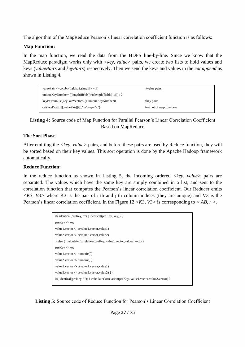
The algorithm of the MapReduce Pearson’s linear correlation coefficient function is as follows:
Map Function:
In the map function, we read the data from the HDFS line-by-line. Since we know that the
MapReduce paradigm works only with <key, value> pairs, we create two lists to hold values and
keys (valuePairs and keyPairs) respectively. Then we send the keys and values in the cat append as
shown in Listing 4.
Listing 4: Source code of Map Function for Parallel Pearson’s Linear Correlation Coefficient
Based on MapReduce
The Sort Phase:
After emitting the <key, value> pairs, and before these pairs are used by Reduce function, they will
be sorted based on their key values. This sort operation is done by the Apache Hadoop framework
automatically.
Reduce Function:
In the reduce function as shown in Listing 5, the incoming ordered <key, value> pairs are
separated. The values which have the same key are simply combined in a list, and sent to the
correlation function that computes the Pearson’s linear correlation coefficient. Our Reducer emits
<K3, V3> where K3 is the pair of i-th and j-th column indices (they are unique) and V3 is the
Pearson’s linear correlation coefficient. In the Figure 12 <K3, V3> is corresponding to < AB, r >.
Listing 5: Source code of Reduce Function for Pearson’s Linear Correlation Coefficient
valuePair <- combn(fields, 2,simplify = F) #value pairs
uniqueKeyNumber=((length(fields))*((length(fields)-1))) / 2
keyPair=unlist(keyPairVector<-(1:uniqueKeyNumber)) #key pairs
cat(keyPair[[i]],valuePair[[i]],"\n",sep="\t") #output of map function
if( identical(preKey, "") || identical(preKey, key)) {
preKey <- key
value1.vector <- c(value1.vector,value1)
value2.vector <- c(value2.vector,value2)
} else { calculateCorrelation(preKey, value1.vector,value2.vector)
preKey <- key
value1.vector <- numeric(0)
value2.vector <- numeric(0)
value1.vector <- c(value1.vector,value1)
value2.vector <- c(value2.vector,value2) }}
if(!identical(preKey, "")) { calculateCorrelation(preKey, value1.vector,value2.vector) }

Page 38 / 75
5.3.2. Classification Module
This section presents the implementation of the kNN function in a three different ways: sequential,
parallel based on multi-core, and parallel based on MapReduce.
5.3.2.1. Sequential:
In order to implement the kNN function in a sequential way, we simply use the knn() function from
the R class package in Listing 6 as follows:
Listing 6: Source Code of kNN function in a Sequential Way
5.3.2.2. Parallel based on Multi-core:
In order to implement the kNN function in a parallel way utilizing all possible cores in one
computer (machine), the high-performance computing with multi-core R package is used. In this
type of parallelization, we do not implement or transform the sequential kNN function, we just
increase the computing power with the multi-core package (including load balancing). [As with
4.3.1.2]
5.3.2.3. Parallel based on MapReduce:
In this section we present the main design for the parallel kNN algorithm based on MapReduce. In
order to transform the sequential kNN as map and reduce functions, the sequential algorithm should
be analyzed to determine which part of the algorithm can or should be parallelized. In the sequential
kNN algorithm, the most intensive computation is the computation of distances with neighbors. The
design of the algorithm originated from a article of Processing kNN Queries in Hadoop [27]. We
face another obstacle, which is the fact that two different data sets need to be fed into MapReduce:
the training set and the test set (Figure 13). This problem is solved using RHadoop again, with the
test set fed to each map and reduce via a distributed cache file. The kNN function is implemented as
a MapReduce job comprising several Mappers and a Reducer. The overview of the map and reduce
function is shown in Figure 13.
traincol<-which( colnames(data)=="A.OTHP3 ")
cluster_raw<-NULL
train<-matrix(data[,traincol],nrow(data),1)
for(i in 1:ncol(data)){
test<-matrix(data[,i],nrow(data),1)
clust<-round(nrow(data)/k,digits=0)
cl <- tapply(numeric(paste(train)), k)
raw_cluster<-knn(train, test, cl$[1,], k, prob=TRUE)
cluster_raw<-c(cluster_raw,raw_cluster) } cluster<-matrix(cluster_raw,nrow(data),ncol(data))

Page 39 / 75
Figure 13: Flow Chart of Parallel kNN Algorithm Based on MapReduce
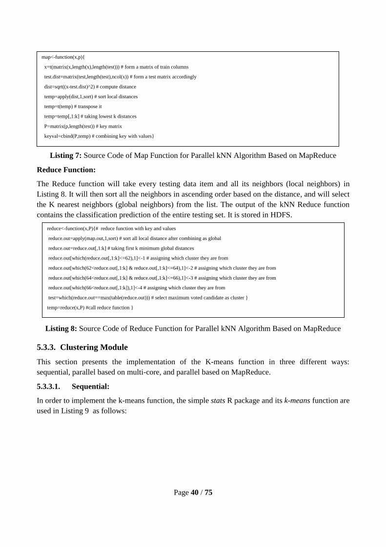
Map Function:
The map functions will be triggered for every training set data item, and will simply compute the
Euclidean distance function. In Listing 7 as illustrated, the distances between all testing sets and
training sets are calculated concurrently through computing nodes, with every node responsible for
calculating the distance between all data items in the complete testing set and a subset of the
training set. Then the results – which are the k-nearest local neighbors – are emitted to the reducer.
Page 40 / 75
Listing 7: Source Code of Map Function for Parallel kNN Algorithm Based on MapReduce
Reduce Function:
The Reduce function will take every testing data item and all its neighbors (local neighbors) in
Listing 8. It will then sort all the neighbors in ascending order based on the distance, and will select
the K nearest neighbors (global neighbors) from the list. The output of the kNN Reduce function
contains the classification prediction of the entire testing set. It is stored in HDFS.
Listing 8: Source Code of Reduce Function for Parallel kNN Algorithm Based on MapReduce
5.3.3. Clustering Module
This section presents the implementation of the K-means function in three different ways:
sequential, parallel based on multi-core, and parallel based on MapReduce.
5.3.3.1. Sequential:
In order to implement the k-means function, the simple stats R package and its k-means function are
used in Listing 9 as follows:
map<-function(x,p){
x=t(matrix(x,length(x),length(test))) # form a matrix of train columns
test.dist=matrix(test,length(test),ncol(x)) # form a test matrix accordingly
dist=sqrt((x-test.dist)^2) # compute distance
temp=apply(dist,1,sort) # sort local distances
temp=t(temp) # transpose it
temp=temp[,1:k] # taking lowest k distances
P=matrix(p,length(test)) # key matrix
keyval=cbind(P,temp) # combining key with values}
reduce<-function(x,P){# reduce function with key and values
reduce.out=apply(map.out,1,sort) # sort all local distance after combining as global
reduce.out=reduce.out[,1:k] # taking first k minimum global distances
reduce.out[which(reduce.out[,1:k]<=62),1]<-1 # assigning which cluster they are from
reduce.out[which(62<reduce.out[,1:k] & reduce.out[,1:k]<=64),1]<-2 # assigning which cluster they are from
reduce.out[which(64<reduce.out[,1:k] & reduce.out[,1:k]<=66),1]<-3 # assigning which cluster they are from
reduce.out[which(66<reduce.out[,1:k]),1]<-4 # assigning which cluster they are from
test=which(reduce.out==max(table(reduce.out))) # select maximum voted candidate as cluster }
temp=reduce(x,P) #call reduce function }

Page 41 / 75
Listing 9: Source Code of K-means function in a Sequential Way
5.3.3.2. Parallel based on Multi-core:
In order to implement the K-means function in a parallel way utilizing all possible cores in one
computer (machine), the high-performance computing with multi-core package R is used. In this
type of parallelization, we do not implement or transform the sequential kNN function; we simply
increase the computing power with the multi-core package (including load balancing). [As with
4.3.1.2]
5.3.3.3. Parallel based on MapReduce:
In this section we present the main design for the parallel K-means algorithm based on MapReduce.
In order to transform the sequential K-means as map and reduce functions, the sequential algorithm
should be analyzed to determine which part of the algorithm can or should be parallelized. In the
sequential K-means algorithm, the most intensive computation is the computation of distances [25].
In each iteration, a total of (nk) distance computations would be required, where n is the number of
objects and k is the number of clusters being created. It is obvious that the distance computation
between one object with the centers is independent of the distance computations between other
objects with the corresponding centers. Therefore, distance computations between different objects
and centers can be executed in parallel.
For the each iteration, the new centers (which are used in the next iteration) should be
renewed with new ones. Because of the update process, the iterative processes (iterative loop) must
be carried out serially, such that each iteration is one MapReduce job. In order to do this, the
RHadoop interface is used because it has the rhdfs package that allows us to access a stored file on
HDFS. Another advantage of using RHadoop is that it provides full control of Hadoop through the
R interface, thanks to the rmr package as described in background section. In RHadoop, each task is
a sequence of many thousands of (key, value) pairs. Before running the map and reduce expression
– and before any (key, value) pairs have been read – RHadoop will evaluate expressions in the
setup. The setup expression is similar to [2, 3] Java, where the user can provide the Java Archive
(jar) files to be uploaded before the job is executed.
clust<-list()
nodes=150
#for(i in 1:ncol(data)){
for(i in 1:nodes){
nlevel <-nrow(tapply(1:NROW(data), data[,i], function(x) length(unique(x))))
k_effec<-min(k,nlevel)
clust[[i]] <- kmeans(as.numeric(paste((data[,i]))), k_effec)}
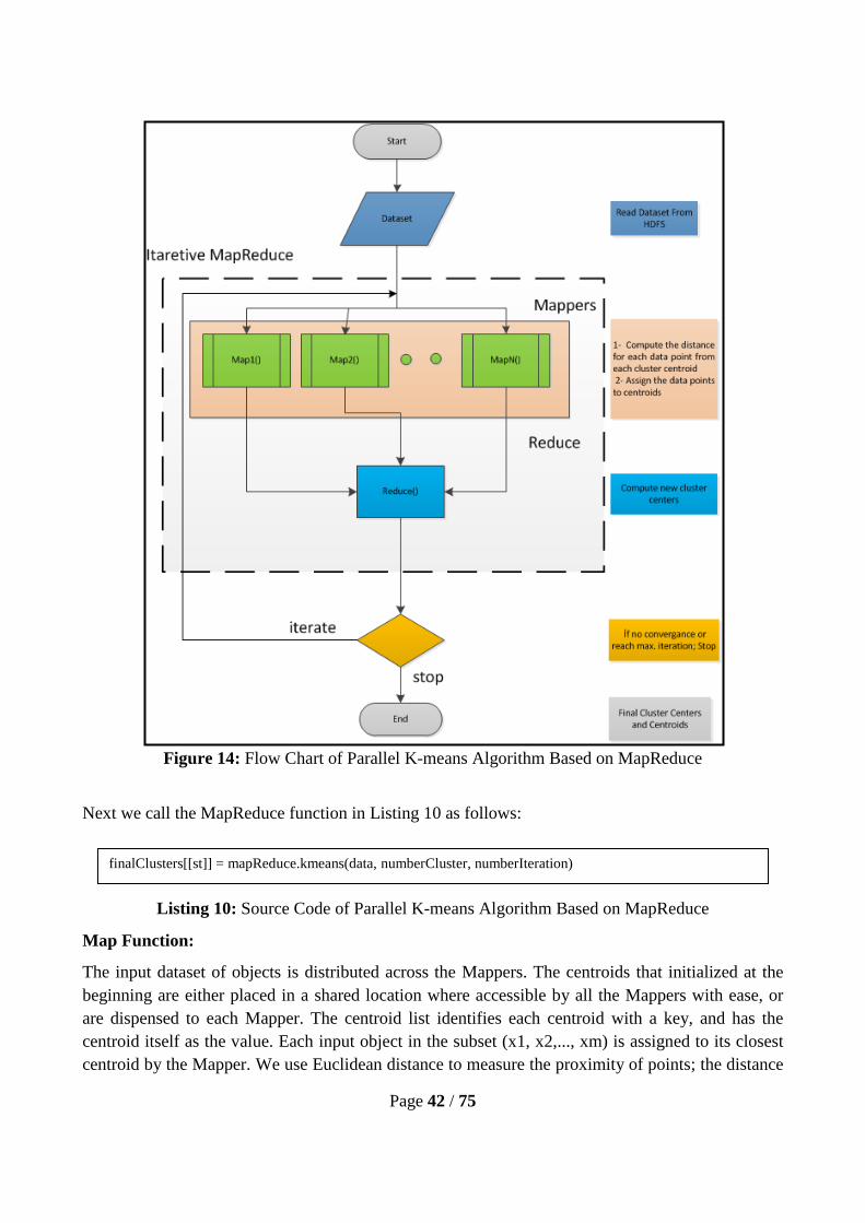
Page 42 / 75
Figure 14: Flow Chart of Parallel K-means Algorithm Based on MapReduce
Next we call the MapReduce function in Listing 10 as follows:
Listing 10: Source Code of Parallel K-means Algorithm Based on MapReduce
Map Function:
The input dataset of objects is distributed across the Mappers. The centroids that initialized at the
beginning are either placed in a shared location where accessible by all the Mappers with ease, or
are dispensed to each Mapper. The centroid list identifies each centroid with a key, and has the
centroid itself as the value. Each input object in the subset (x1, x2,..., xm) is assigned to its closest
centroid by the Mapper. We use Euclidean distance to measure the proximity of points; the distance
finalClusters[[st]] = mapReduce.kmeans(data, numberCluster, numberIteration)

Page 43 / 75
between the each data and all the other data found in the training set is calculated. Then, the object
is assigned to it’s the most closest cluster of centroid. When entire object sets are assigned to the
closest cluster of centroids, the Mapper emits all the input object sets (and the centroids that they
are assigned as well) to the reducer as was shown in Figure 14.
Listing 11: Source Code of Map Function for Parallel K-means Algorithm Based on MapReduce
In Listing 11, distance criterion used. The map function returns keyval which is all the center-point
pairs.
Reduce function:
The Reduce function calculates new centroid values using the output the (key, value) pairs from the
Mappers in Listing 12. For each centroid, the reducer calculates a new value based on the objects
assigned to it in that iteration. This new centroid list is emitted as the reducer’s output in the form of
new (key, value) pairs.
Listing 12: Source Code of Reduce Function for Parallel K-means Algorithm Based on MapReduce
Iteration Function:
The decision about whether or not the Reduce outputs represent the final cluster centers is handled
in R as a simple iteration function ( in Listing 13), which calculates the change in centroid positions
and decides (based on convergence) whether to re-invoke the MapReduce job again or emit the
final result HDFS.
Listing 13: Source Code of Iteration Function for Parallel K-means Algorithm Based on
MapReduce
map = function(., Dpoints){
closest = { if (is.null(centers))
else { distance = calculateDistance(centers, Dpoints) nearest = max.col(-distance)}}
if (in.memory.combine) keyval(closest, rbind(1, Dpoints))
else keyval(closest, Dpoints) }
reduce = {if ((!in.memory.combine))
function(., P) t(as.matrix(apply(Dpoints, 2, mean)))
else function(k, Dpoints) keyval( k, t(as.matrix(apply(Dpoints, 2, sum)))) }
calculateDistance = function(centers, Dpoints) {
transposed=t(Dpoints)
apply(centers,1,function(i)colSums((transposed-i)^2)) }

Page 44 / 75
Distance Function:
The distance function simply computes all the distances between a matrix of centers and a matrix of
data points. The apply() function is used for this and it is presented in Listing 14.
Listing 14: Source Code of Distance Function for Parallel K-means Algorithm Based on
MapReduce
5.4. Implementation of the Case Study
5.4.1. Case Study
This section details the implementation of the case study, which utilizes the three different modules
and the decision tree function.
5.4.1.1. Implementation of the Case Study
This section presents the implementation of a case study scenario that uses the previous standalone
algorithms (sequential, parallel based on multicore and MapReduce) concurrently in order to extract
knowledge. The data preparation and the decision tree implementation were done using only
sequential R.
Decision-tree:
This section presents the sequential implementation of the CART decision tree function. In order to
implement the CART decision tree function, the R rpart() package and its rpart() function is used.
Listing 15 illustrates the usage of the tree function is as follows:
Listing 15: Source Code of Sequential Decision Tree
calculateDistance = function(centers, Dpoints) {
transposed=t(Dpoints)
apply(centers,1,function(i)colSums((transposed-i)^2)) }
tree<-function(x){
dat<-cbind(cluster[,ncol(cluster)],volt.knn[,temp.volt[x]],cons.kmeans[,temp.cons[x]]) # form a matrix of dependent and #independent
variables
colnames(dat)<-c("production.cluster","voltage.class","consumption.cluster") # give the column names
dat<-as.data.frame(dat) # identify dat as data frame
d.tree = rpart(production.cluster ~ voltage.class + consumption.cluster, method="class",data=dat) # calculate decision tree
return(d.tree) } # return decision tree

Page 45 / 75
The workflow of the case study scenario work-flow was shown in Figure 9. In order to
perform this workflow, the data sets are first prepared based on how they will be used. The voltage
and consumption data sets are merged based on voltage nodes, the transmission data is transformed
to a numeric matrix, and finally the production data set matrix is transformed to its transposed and
numeric matrix.
For Platform 1 and Platform 2:
After all the data sets are ready for the data mining process, three R processes are run
simultaneously and each process is used to carry out one part (task) of the data mining process. The
statistical module (Pearson’s linear correlation function) is applied to the merged consumption and
voltage data set. The Pearson’s linear correlation coefficient values are found between the
consumption and voltage values; based on voltage data. The classification module is applied to the
voltage data set and the clustering module is applied to the consumption data set. After all three
processes are completed, each module's results are written to .csv files separately—to be used later
in the decision-tree phase of data mining process. Then all three outputs are merged as a single .csv
file to be used as decision weights in the decision-tree phase of data mining process.
The clustering module is applied to the production data as well, but in a separate run, and its
output is written to a different .csv file to be used as a training data set in the decision-tree phase of
the data mining process.
After the decision weights and training data set are produced, the CART decision-tree is
applied as the last part of the data mining process; production clusters are predicted and the result is
plotted as CART decision-tree.
For Platform 3:
Once all the data sets are ready for the data mining process, three different MapReduce Jobs are run
simultaneously and each job is used to carry out one part (task) of data mining process. The
statistical module (Pearson’s linear correlation coefficient function) is applied to the merged
consumption and voltage data set as a MapReduce job. The Pearson’s linear correlation coefficient
values between consumption and voltage values are found; based on voltage data. The classification
module is applied to the voltage data set as a MapReduce job, and the clustering module is applied
to the consumption data set as a MapReduce job. Once all three MapReduce jobs are completed,
each MapReduce job's results are written to .csv files into HDFS separately—to use later in the
decision-tree phase of data mining process. Then all three outputs are merged into a single .csv file
to be used as decision weights in the decision-tree phase of the data mining process.
The clustering module is applied to the production data as well, but in a separate run, and its
output is written to a different .csv file in HDFS—to be used as a training data set in the decision-
tree phase of the data mining process.
After decision weights and the training data set are produced, the CART decision-tree is
applied as a last part of the data mining process; production clusters are predicted, and the result is
plotted as a CART decision-tree.

Page 46 / 75
Chapter 6
6. Evaluation of the Study
This evaluation chapter has two main parts: the first part is the evaluation of the algorithms for the
three chosen modules, and the second part is an evaluation in the context of the use case scenario.
The study of this scenario consists of the concurrent running of the modules examined earlier.
6.1. Evaluation of the Standalone Modules
All of the functions in the statistical module (Pearson’s linear correlation coefficient) are
implemented for all three different platforms separately. All the functions are run five times on each
platform; and the average results are taken into account to provide more accurate results. In this
experiment, all the factors remain the same except the size of the data set. The data set size varies
between 693, 1000, 1350, and 2025 nodes; these being equivalent to data sizes of 2.78E+06,
1.47E+07, 1.87E+07 and 4.22E+07 respectively.
All the functions in the classification module are implemented for all three platforms
separately. All the functions are run five times on each platform, and the average measured times
are taken into account to provide more accurate results. In this experiment, all the factors remain
same except the size of the data set. The data set size varies between 676, 1352, 2704, and 6078
nodes; these being equivalent to data sizes of 4.96E+06, 9.39E+06, 3.75E+07 and 8.44E+07
respectively. In order to measure the efficiency and scalability of the parallel platforms, different
numbers of cores (between 1 and 4 for platform-2) and different numbers of nodes (from 1 to 3 for
platform-3) are used and compared. For all platforms the class number (K=4) is used.
All the functions in the clustering module are implemented for all three different platforms
separately. All the functions are run five times on each platform, and the average measured times
are taken into account to provide more accurate results. In this experiment, all the factors remain the
same except the size of the data set. The data set size varies between 500, 974, 1948 and 5844
nodes; these being equivalent to 3.47E+06, 6.76E+06, 2.70E+07 and 8.11E+07 respectively. In
order to measure the efficiency and scalability the parallel platforms, different numbers of cores
(between 1 and 4 for platform-2) different numbers of nodes (between 1 and 3 for platform-4) are
used and compared. For all platforms the cluster number (K = 5) and number of iterations (5) are
used.
6.1.1. Performance
This section presents the evaluation of the Elapsed Time performance metric for the three different
modules as depicted in Table 3.

Page 47 / 75
Method
Statistical Module Classification
Module Clustering Module
# of Data Avg.
Elapsed Time ( s )
# of Data Avg.
Elapsed Time ( s )
# of Data Avg.
Elapsed Time ( s )
R
4.86E+04 2,602 4.69E+06 138,666 3.47E+06 15,349
1.47E+07 37,427 9.39E+06 311,803 6.76E+06 24,924
1.87E+07 105,101 3.75E+07 537,607 2.70E+07 114,953
4.22E+07 245,623 8.44E+07 1375,213 8.11E+07 540,279
Multi-core R
4.86E+04 38 4.69E+06 78,865 3.47E+06 11,560
1.47E+07 26,499 9.39E+06 141,161 6.76E+06 19,821
1.87E+07 59,232 3.75E+07 260,322 2.70E+07 78,556
4.22E+07 171,284 8.44E+07 410,322 8.11E+07 226,895
Hadoop + R
4.86E+04 3 4.69E+06 118 3.47E+06 43
1.47E+07 62 9.39E+06 165 6.76E+06 57
1.87E+07 73 3.75E+07 223 2.70E+07 94
4.22E+07 128 8.44E+07 312 8.11E+07 189
Table 3: Average Elapsed Time Spends For Standalone Modules
The figures (graphs) are presented here before the explanatory text, to make it easy to refer back to
them when reading the subsequent explanations:
Figure 15 : (a) Performance for (b) Performance for (c) Performance for
Statistical Module Classification Module Clustering Module
In the Figure 15 the X-axis represents the number of voltage values in the data set and the Y-axis
represents the elapsed time in seconds.
The actions represented here are loading of the dataset into memory, calculating Pearson’s
linear correlation coefficient values for the selected node pairs (a), calculating kNN class values for
each node (b), calculating K-mean cluster values for each node (c), and writing the result to HDFS
or to hard drive.
Figure 15 (a) shows that for statistical module, Hadoop+R1 are no faster than multi-core R
and single R for small data sets. Figure 15 (b) and (c) show that for the classification module and
1 Hadoop+R will be used for the rest of the paper to indicate for integration between R and Hadoop either with
RHadoop or Apache Hadoop Streaming.

Page 48 / 75
the clustering module, respectively, multi-core R and single R are faster than Hadoop+R for very
small data sets. This is because Hadoop uses the MapReduce framework, the data is distributed into
slave nodes in the cluster, and – after the map function is completed – the results are gathered for
the reduce function; all of which obviously affects the elapsed time. Also, the Hadoop+R elapsed
time includes setup time, map and reduce time, and cleanup time. In addition to these factors for (b)
and (c), since RHadoop uses the rmr package to provide integration between R and the Hadoop
framework, RHadoop needs time to initialize some required libraries (such as the native-hadoop
and native-zlib libraries) before it triggers the Hadoop job.
Figure 15 (a, b, and c) shows that with increasing of data set size, the R elapsed time
increases dramatically, unlike Multi-core R and Hadoop+R. The performances of Hadoop+R and
Multi-core R are quite similar, but Hadoop+R is slightly better, and the Hadoop+R performance
gets even better (relatively) as the size of the data set increases. It is quite possible to determine –
based on the slopes of the lines – that Hadoop+R will continue to perform better than R and (to a
lesser extent multi-core R) as the data set size increases. But it is clear that with bigger data set
sizes, Hadoop performs better as expected.
Our conclusion is that, across the three modules, parallelization with Hadoop+R offers
consistently better performance than the serial algorithm (R) and multi-core R for reasonable data
set sizes. However, Hadoop+R is not a good choice for small data set sizes due to setup time, clean-
up time and overloading.
6.1.2. Memory Usage
This section presents the evaluation of the Memory Usage performance metric for the three
different modules as illustrated in Table 4.
Method
Statistical Module Classification Module Clustering Module
# of Data Memory
Consumption (Mb)
# of Data Memory
Consumption (Mb)
# of Data Memory
Consumption (Mb)
R
4.86E+04 158 4.69E+06 325 3.47E+06 225
1.47E+07 435,70 9.39E+06 669 6.76E+06 295
1.87E+07 772,80 3.75E+07 837 2.70E+07 1297
4.22E+07 1255 8.44E+07 1658 8.11E+07 1869
Multi-core R
4.86E+04 164,60 4.69E+06 560 3.47E+06 365
1.47E+07 516 9.39E+06 495 6.76E+06 395
1.87E+07 1127 3.75E+07 1055 2.70E+07 414
4.22E+07 1702 8.44E+07 1280 8.11E+07 689
Hadoop + R
4.86E+04 390,50 4.69E+06 266 3.47E+06 256,02
1.47E+07 362,16 9.39E+06 301 6.76E+06 291,02
1.87E+07 399,84 3.75E+07 321 2.70E+07 301,22
4.22E+07 408,30 8.44E+07 450 8.11E+07 382,07

Page 49 / 75
Table 4: Memory Consumption for Standalone Modules
The figures (graphs) are presented here before the explanatory text, to make it easy to refer
back to them when reading the subsequent explanations:
Figure 16 : (a) Memory Usage for (b) Memory Usage for (c) Memory Usage for
Statistical Module Classification Module Clustering Module
In Figure 16, the X-axis represents the number of nodes and the Y-axis represents the
Memory Usage time in megabytes. The actions represented here are loading of the dataset into
memory, calculating Pearson’s linear correlation coefficient values for the selected node pairs (a),
calculating kNN class values for each node (b), calculating k-mean cluster values for each node,
and writing the result into HDFS or to hard drive.
Figure 16 indicates that the best option based on memory consumption is Hadoop+R
regardless of the module. Compared with R and multi-core R, the memory usage for Hadoop+R
does not change dramatically with increasing data set size. Although it may consume much more
memory at the beginning, the memory usage does not change significantly as the data set size
increases (it has very low increment). As the data set size increases, Hadoop begins to split and
distribute the data more efficiently such that it is almost 3 or 4 times more efficient (quite
impressive) than sequential R and multi-core R respectively.
Our conclusion is that, for the three modules, Hadoop+R is the best option based on memory
consumption. This is because Hadoop distributes small chunks of data to slave nodes such that the
memory usage is extremely low, even for huge data set sizes. As such, memory usage is a
significant factor in cluster loading, because Hadoop views the clusters only with respect to
memory [2, 3]. Since every task node starts a Java virtual machine, memory usage is related to the
number of running TaskTrackers, so there is a risk of the Linux Out-Of-Memory (OOM) randomly
killing processes if you run too many TaskTrackers. The other thing to keep in mind is that R is
memory bound (i.e. requires your whole data set to be held in RAM), therefore processing an 8 GB
data set on a 3.8 GB machine would be impossible; but there is no such problem with Hadoop+R
which splits the data and distributes it efficiently.

Page 50 / 75
6.1.3. Accuracy
Because the statistical module results and classification module results are same for each platform,
they are not presented here (see Appendix A). However, the results of the K-means algorithm are
slightly different each time because it starts randomly; therefore in Figure 17 we present the
comparative results for clustering module on the different platforms. The different colors represent
the different clusters that result of clustering module (K-means function).
Figure 17: (a) Platform-1 (b) Platform-2
(c) Platform-3
6.1.4. Efficiency
This section presents the evaluation of the efficiency metric (including speed-up) of the three
different modules separately.
a) Speed-up
Figure 18 shows the results for the statistical module (Pearson’s linear correlation coefficient) for

Page 51 / 75
multi-core (platform-2, shown as squares) and Hadoop cluster (platform-3, shown as triangles). The
X-axis represents the number of cores and the Y-axis represents the speed-up, and in this
experiment the number of cores or nodes is varied between 1 and 4. The blue line indicates the ideal
acceleration, which is difficult to achieve in practice, but the purple lines (data set size of 6078)
come close to this ideal for all numbers of cluster nodes or nodes. It is clear that the speed-up is not
so good for small data set sizes, but in all cases the speed-up seems to increase as the number of
cores or nodes increases.
Figure 18: Speed-up for Statistical Module on Platform-2 and -3
Figure 19 shows the results for the classification module (kNN function) for multi-core
(platform-2, shown as squares) and Hadoop cluster (platform-3, shown as triangles). The X-axis
represents the number of cores and the Y-axis represents the speed-up. In this experiment, the
number of cores is varied between 1 and 4. The blue line indicates the ideal acceleration, which is
difficult to achieve in practice, but the purple lines (data set size of 6078) come close to this ideal
for all numbers of cluster nodes. It is clear that the speed-up is not so good for small data set sizes,
but in all cases the speed-up seems to increase as the number of cores increases.

Page 52 / 75
Figure 19: Speed-up for Classification Module on Platform-2 and -3
Figure 20 shows the results for the Clustering module (K-means function) for multi-core
(platform-2, shown as squares) and Hadoop cluster (platform-3, shown as triangles). The X-axis
represents the number of cores and the Y-axis represents the speed-up. In this experiment, the
number of cores is varied between 1 and 4. The dark red line indicates the ideal acceleration, which
is difficult to achieve in practice, but the green lines (data set size of 5844) come close to this ideal
– in terms of the slopes of the lines – for all numbers of cluster nodes. It is clear that the speed-up is
not so good for small data set sizes, but in general the speed-up seems to increase as the number of
cores increases.
Figure 20: Speed-up for Clustering Module on Platform-2 and -3
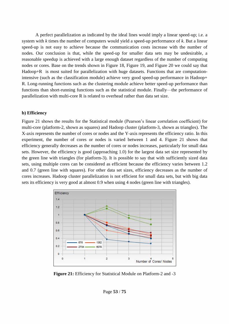
Page 53 / 75
A perfect parallelization as indicated by the ideal lines would imply a linear speed-up; i.e. a
system with k times the number of computers would yield a speed-up performance of k. But a linear
speed-up is not easy to achieve because the communication costs increase with the number of
nodes. Our conclusion is that, while the speed-up for smaller data sets may be undesirable, a
reasonable speedup is achieved with a large enough dataset regardless of the number of computing
nodes or cores. Base on the trends shown in Figure 18, Figure 19, and Figure 20 we could say that
Hadoop+R is most suited for parallelization with huge datasets. Functions that are computation-
intensive (such as the classification module) achieve very good speed-up performance in Hadoop+
R. Long-running functions such as the clustering module achieve better speed-up performance than
functions than short-running functions such as the statistical module. Finally—the performance of
parallelization with multi-core R is related to overhead rather than data set size.
b) Efficiency
Figure 21 shows the results for the Statistical module (Pearson’s linear correlation coefficient) for
multi-core (platform-2, shown as squares) and Hadoop cluster (platform-3, shown as triangles). The
X-axis represents the number of cores or nodes and the Y-axis represents the efficiency ratio. In this
experiment, the number of cores or nodes is varied between 1 and 4. Figure 21 shows that
efficiency generally decreases as the number of cores or nodes increases, particularly for small data
sets. However, the efficiency is good (approaching 1.0) for the largest data set size represented by
the green line with triangles (for platform-3). It is possible to say that with sufficiently sized data
sets, using multiple cores can be considered as efficient because the efficiency varies between 1.2
and 0.7 (green line with squares). For other data set sizes, efficiency decreases as the number of
cores increases. Hadoop cluster parallelization is not efficient for small data sets, but with big data
sets its efficiency is very good at almost 0.9 when using 4 nodes (green line with triangles).
Figure 21: Efficiency for Statistical Module on Platform-2 and -3

Page 54 / 75
Figure 22 shows the results for the Classification module (kNN function) for multi-core
(platform-2, shown as squares) and Hadoop cluster (platform-3, shown as triangles). The X-axis
represents the number of cores and the Y-axis represents the efficiency. In this experiment, the
number of cores or nodes is varied between 1 and 4. The efficiency generally decreases as the
number of cores increases, particularly for small data sets. However, the efficiency is good
(approaching 1.0) for the largest data set size represented by the green lines. It is clear that using
Hadoop cluster is not a good idea for small data sets since the speed-up is not so great. The graph
shows a good result for the biggest data set (green line with triangles) regardless of number of
cluster nodes; it is quite close to the ideal of 1 and at some points is even better. It is possible to say
that with a sufficiently huge data set and using multiple cores, it can be considered as efficient
because the efficiency ranges between 1.4 and 0.8 (green line with squares). For other sizes of data
set, efficiency decreases as the number of cores or nodes increase.
Figure 22: Efficiency for Classification Module on Platform-2 and -3
Figure 23 shows the results for the Clustering module (K-means function) for multi-core
(platform-2, shown as squares) and Hadoop cluster (platform-3, shown as triangles). The X-axis
represents the number of cores and the Y-axis represents the efficiency. In this experiment, the
number of cores is varied between 1 and 4. The graph shows that efficiency generally decreases as
the number of cores increases, particularly for small data sets. However, the efficiency is good
(approaching 1.0) for the largest data set size represented by the green lines. It is possible to say that
with sufficiently sized data sets and using multiple cores, it can be considered as efficient at 0.6
(green line with squares). The graph shows that using Hadoop cluster is not efficient for small data
sets, but with big data sets the efficiency is quite good (green line with triangles, at 0.7 and 0.6,
respectively) and is even better than the multi-core result.

Page 55 / 75
Figure 23: Efficiency for Clustering Module on Platform-2 and -3
Our conclusion is that while it is not easy to reach the ideal efficiency for small data sets
(regardless of our parallelization methods); with a sufficiently large data set it is possible to achieve
a good degree of efficiency. We could say that Hadoop+R (platform-3) is slightly more efficient
than multi-core R (platform -2) based on the efficiency figures.
6.1.5. Scale-up
This section presents the evaluation of scale-up metric of the three different modules separately.
Figure 24 : (a) Scale-up for (b) Scale-up for (c) Scale-up for
Statistical Module on Classification Module on Clustering Module on
Platform-2 and -3 Platform-2 and -3 Platform-2 and -3
Figure 24 (a), (b), and (c) shows scale-up for statistical module, classification module, and
clustering module respectively. The X-axis represents the number of cores or nodes and the Y-axis
represents the scale-up. In this experiment, the number of cores or nodes is varied between 1 and 4.
The blue line indicates the ideal scalability, which is constant. It is reasonable to say that the system
has low scalability for multicore R (platform-2) for all three modules (red lines). On the other hand,
it is clearly reasonable to say that Hadoop+R has high scalability (albeit, the scale-up ratio is
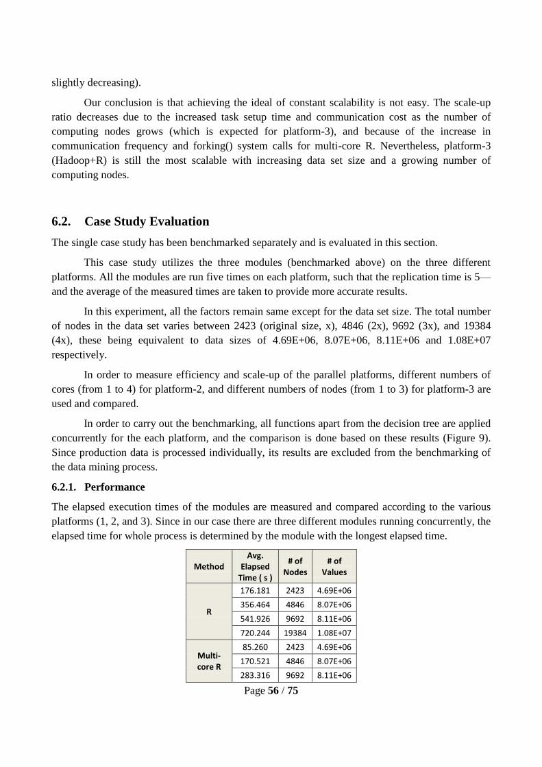
Page 56 / 75
slightly decreasing).
Our conclusion is that achieving the ideal of constant scalability is not easy. The scale-up
ratio decreases due to the increased task setup time and communication cost as the number of
computing nodes grows (which is expected for platform-3), and because of the increase in
communication frequency and forking() system calls for multi-core R. Nevertheless, platform-3
(Hadoop+R) is still the most scalable with increasing data set size and a growing number of
computing nodes.
6.2. Case Study Evaluation
The single case study has been benchmarked separately and is evaluated in this section.
This case study utilizes the three modules (benchmarked above) on the three different
platforms. All the modules are run five times on each platform, such that the replication time is 5—
and the average of the measured times are taken to provide more accurate results.
In this experiment, all the factors remain same except for the data set size. The total number
of nodes in the data set varies between 2423 (original size, x), 4846 (2x), 9692 (3x), and 19384
(4x), these being equivalent to data sizes of 4.69E+06, 8.07E+06, 8.11E+06 and 1.08E+07
respectively.
In order to measure efficiency and scale-up of the parallel platforms, different numbers of
cores (from 1 to 4) for platform-2, and different numbers of nodes (from 1 to 3) for platform-3 are
used and compared.
In order to carry out the benchmarking, all functions apart from the decision tree are applied
concurrently for the each platform, and the comparison is done based on these results (Figure 9).
Since production data is processed individually, its results are excluded from the benchmarking of
the data mining process.
6.2.1. Performance
The elapsed execution times of the modules are measured and compared according to the various
platforms (1, 2, and 3). Since in our case there are three different modules running concurrently, the
elapsed time for whole process is determined by the module with the longest elapsed time.
Method Avg.
Elapsed Time ( s )
# of Nodes
# of Values
R
176.181 2423 4.69E+06
356.464 4846 8.07E+06
541.926 9692 8.11E+06
720.244 19384 1.08E+07
Multi-core R
85.260 2423 4.69E+06
170.521 4846 8.07E+06
283.316 9692 8.11E+06

Page 57 / 75
401.321 19384 1.08E+07
Hadoop + R
128 2423 4.69E+06
185 4846 8.07E+06
218 9692 8.11E+06
273 19384 1.08E+07
Table 5: Average Elapsed Time Spent for data mining processes
Elapsed Time Spent: “Wall Clock” time is the total elapsed time from start to end of a timed task.
In Figure 25 for the elapsed time spent during the data mining process, the X-axis represents
the total number of data set nodes and the Y-axis represents the elapsed time spent in seconds.
Figure 25: Comparison of Elapsed Time Spent by Different Platforms for the Data Mining
Processes
The actions represented here are the loading of the dataset into memory, calculating kNN
classes for voltage data values for each node, calculating K-means cluster values for consumption
data, calculating Pearson’s linear correlation coefficient values for dataset-1 given in Figure 9, and
writing the result to HDFS or to hard drive. It is clear that single R and multi-core R are much faster
than Hadoop+R for very small data set sizes. This is because Hadoop uses the MapReduce
framework, so the data is distributed into clusters and finally the results are gathered—all of which
obviously affects the elapsed time spent. Also, the elapsed time spent includes setup time, map and
reduce time, and cleanup time. Lastly, since RHadoop uses the rmr package to provide integration
between R and the Hadoop framework, it needs time to initialize some required libraries – such as
native-hadoop and native-zlib – before it triggers the Hadoop job.
The graph shows that the R elapsed time increases dramatically (more so than Hadoop+R
and Multi-core R) as the data set size increases. The Hadoop+R and multi-core R performances are
quite similar, but Hadoop+R is much better. Based on the slopes of the lines, it is possible to say
that Hadoop+R will perform best, single R will perform worst, and multi-core R will be somewhere
in between for increasing data set sizes.

Page 58 / 75
6.2.2. Memory Consumption
The memory consumption in megabytes of programs are measured and compared based on various
platforms (in our case: platform 1, 2, and 3).
While memory consumption values are calculated for Hadoop Cluster (platform-3), the
tasks’2 memory consumption values are aggregated so that the total memory consumption is
calculated; and since the three different modules are running concurrently, their memory
consumption values are aggregated so that total memory consumption is calculated.
Method Memory
Consumption ( Mb )
# of Nodes
# of Values
R
1013 2423 4.69E+06
1766 4846 8.07E+06
2507 9692 8.11E+06
3447 19384 1.08E+07
Multi-core R
1505 2423 4.69E+06
1680 4846 8.07E+06
2390 9692 8.11E+06
3199 19384 1.08E+07
Hadoop + R
771,598 2423 4.69E+06
859,056 4846 8.07E+06
981,911 9692 8.11E+06
1285,553 19384 1.08E+07
Table 6: Memory Consumption for Data Mining Processes
In Figure 26 for memory consumption during the data mining process, the X-axis represents
the total number of values (nodes) of the data set and the Y-axis represents the memory
consumption.
2 Master node runs a JobTracker instance, which accepts Job requests from clients. TaskTracker instances run on
slave nodes and TaskTracker forks separate Java process for task instances ( these are the tasks) [2,3]

Page 59 / 75
Figure 26: Comparison of Memory Consumption by Different Platforms for the Data Mining
Processes
The actions represented here are the loading of the dataset into memory, calculating kNN
classes for voltage data values for each node, calculating K-means cluster values for consumption
data, calculating Pearson’s linear correlation coefficient values for dataset -1 in Figure 9, and
writing the result to HDFS or to hard drive. The graph shows that the best option based on memory
consumption is Hadoop+R, which does not consume significantly more memory as the data set size
increases. Whereas Hadoop+R starts a Java virtual machine for every task node, multi-core R
spawns a child process which uses separate memory. R and multi-core R use more memory then
Hadoop+R, their memory usage increases more significantly as the size of the data set increases.
Hadoop uses data parallelization to distribute small chunks of data to slave nodes, such that memory
usage is extremely low even for huge amount of data sets.
6.2.3. Accuracy
Because the statistical module results and classification module results are same for each platform,
they are not presented here (see Appendix A). However, the results of the K-means algorithm are
slightly different each time because it starts randomly; therefore a comparison was done between
the results for clustering modules on different platforms. Figure 27 shows an example result of
clustering module (K-means clusters) for node A.OTHP3 on the platforms as follows:
Figure 27: (a) Platform-1 (b) Platform -2

Page 60 / 75
(c) Platform-3
6.2.4. Efficiency
In order to the calculate efficiency of the platforms, first the speed-up of the platforms are
calculated and compared as follows:
a) Speed-up
Figure 28 shows the results for the data mining process for multi-core (platform-2, shown as
squares) and Hadoop cluster (platform-3, shown as triangles). The X-axis represents the number of
cores or nodes and the Y-axis represents the speed-up ratio. In this experiment, the number of cores
or nodes is varied between 1 and 4. The blue line indicates the ideal acceleration, which is difficult
to achieve in practice. While the observed acceleration is not ideal, there is some acceleration,
which seems to get better with increasing cluster size (number of nodes) and bigger data set size.
While using the Hadoop cluster is not a good idea for small data sets (actually it is slower than the
sequential one), the angle of the purple line representing the largest data set is quite close to that of
the ideal line for all numbers of cluster nodes.

Page 61 / 75
Figure 28: Speed-up for Data Mining Processes on Platform-2 and -3
b) Efficiency
Figure 29 shows the results for the data mining process for multi-core (platform-2, shown as
squares) and Hadoop cluster (platform-3, shown as triangles). The X-axis represents the number of
cores or nodes and the Y-axis represents the efficiency ratio. In this experiment, the number of
cores or nodes is varied between 1 and 4. It is apparent that for small data set sizes the efficiency
decreases as the number of nodes increases, but the process is relatively efficient (never below 0.8
compared with an ideal of 1) for larger data sets regardless of the number of nodes.
Figure 29: Efficiency for Data Mining Processes on Platform-2 and -3

Page 62 / 75
6.2.5. Scale-up
Since we used two different parallelization ways – platform-2 and platform-3 – two different Scale-
up ratios are calculated then compared.
Figure 30 shows the results for the data mining process for multi-core (platform-2, shown as
a red line) and Hadoop cluster (platform-3, shown as a green line). The X-axis represents the
number of cores or nodes and the Y-axis represents the scale-up ratio. In this experiment, the
number of cores or nodes is varied between 1 and 4. The blue line indicates the ideal scalability
which is constant. The red line (platform-2, multi-core) shows that the system is not scalable as the
number of core nodes increases—probably as a result of more child processes and increased
overlapping. The green line (platform-3, Hadoop+R) shows much better scalability, similar to the
ideal indicated by blue line.
Figure 30: Scale-up for Data Mining Processes on Platform-2 and -3
Decision Tree Result of the Case Study
The decision tree result is presented in Figure 31. This graph shows the final pattern (our
knowledge) of how the production clusters are predicted.

Page 63 / 75
Figure 31 : Prediction of Production Clusters by Cart Decision Tree
In this graph there are seven end nodes (numbered 2, 6, 7, 9, 10, 12 and 13) which represent
the predicted production clusters3 (numbered 1, 3, and 4). There are six decision nodes (numbered
1, 3, and 4, 5, 8, and 11) which represent voltage classes and consumption clusters. The graph
shows that if voltage class is 1 or 2 (i.e. < 2.5) then the predicted production cluster will be 1 (i.e.
node 2), and if the voltage class is 3, 4 or 5 (i.e. >=2.5) then the consumption cluster must be
checked. If the consumption cluster is >=3.5 then the production cluster will be 1 (i.e. node 12),
otherwise it is 4 (i.e. node 13). If the consumption cluster is >=2.5 but <3.5, then we will follow the
left path down to production cluster 1 (i.e. node 6). If consumption cluster >=3.5, then the
production cluster will be 3 (i.e. node 7). If the consumption cluster is <2.5, then we will follow
middle path. Here, If consumption cluster <1.5 then production cluster is 3 (i.e. node 9), otherwise
it is 4 (i.e. node 10).
3
Although the number of production clusters are five ( 1, 2, 3, 4,and 5 ) , 2 and 5 clusters are not predicted according to
our decision tree.

Page 64 / 75
Chapter 7
7. Conclusion and Future Work
This chapter summarizes the contributions and presents the conclusions from the evaluations.
Possible future extensions and improvements to parallelization are discussed under the section as a
future work.
Standard data mining algorithms are transformed to parallel processing platforms as
standalone modules. Real-time experiments are conducted to evaluate the efficacy of these
standalone modules in terms of performance, resource usage (Memory), efficiency (including
speed-up), accuracy, and scalability then these modules re-used concurrently to obtain knowledge
from case study.
The results evaluation shows that the standalone modules and the case study exhibit
consistent parallelization results in terms of performance, resource usage, speed up, efficiency, and
scale up.
A considerable observation made in the evaluation was that the input data size is a very
important agent in achieving reasonable speedup when parallelizing using Hadoop cluster. The
evaluation results clearly show that parallelism with Hadoop cluster is the most scalable and the
most efficient way to implement data mining processes with increasing data set size and a growing
number of computing nodes. Parallelization using multiple cores is a good alternative option, but it
is not as scalable as the Hadoop Cluster.
Future work could focus on enhancements to the standalone modules, plus extension and
improvement of the test beds to give more comprehensive and accurate results:
o In the first case (enhancements to standalone modules) the transformation of sequential
algorithms to parallel algorithms could be improved by using better algorithms such as
writing a combiner function for Hadoop. Also, parallelization with multi-cores could be
implemented at a lower level so that load balancing can be fully controlled.

Page 65 / 75
o In the second case (improvement of test beds), performance could be tuned rather than
conducting the experiments using the current “out-of-the-box” configurations. Hadoop
cluster could be tuned in terms of the number of map and reduce tasks, and I/O performance
of the MapReduce job could be improved through customized Hadoop input and output
types. Hadoop cluster could be extended from small cluster to large cluster (e.g., with 20-30
nodes), and for multi-core a more advanced single computer (e.g., with 8-32 cores) could be
used to investigate parallelization.

Page 66 / 75
References
[1] Anand Rajaraman, and Jeffrey D. Ullman. Mining of Massive Datasets. Cambridge University Press
(November 30, 2011), 2011. http://infolab.stanford.edu/~ullman/mmds.html.
[2] Alex Holmes. Hadoop in Practice, 2012. http://www.manning.com/holmes/.
[3] Tom White. Hadoop: The Definitive Guide. Original edition. O’Reilly Media, 2009. http://hadoopbook.com/.
[4] “Welcome to ApacheTM
Hadoop®!” Accessed May 23, 2013. http://hadoop.apache.org/.
[5] Cristina Olaru, Pierre Geurts, and Louis Wehenkel. “Data Mining Tools and Application in Power System
Engineering.” In Proceedings of the 13th Power System Computation Conference, PSCC99, page 324–330,
1999. http://www.montefiore.ulg.ac.be/services/stochastic/pubs/1999/OGW99.
[6] Z.A. Vale, C. Ramos, T. Pinto, and S. Ramos. “Data Mining Applications in Power Systems — Case-studies
and Future Trends.” 1 – 4. Seoul, 2009. doi:10.1109/TD-ASIA.2009.5356830.
[7] Yomara Pires, Jefferson Morais, Claudomir Cardoso, and Aldebaro Klautau. Innovative Applications in Data
Mining. Studies in Computational Intelligence 169. Springer Berlin Heidelberg, 2009.
http://www.springer.com/engineering/computational+intelligence+and+complexity/book/978-3-540-88044-8.
[8] “Australian Bureau of Statistics.” Accessed June 14, 2013.
http://www.abs.gov.au/websitedbs/d3310114.nsf/Home/Home?OpenDocument.
[9] Pang-Ning Tan, Michael Steinbach, and Vipin Kumar. Introduction to Data Mining. International Edition.
Pearson, 2005.
[10] Steven W. Blume. Electric Power System Basics for the Nonelectrical Professional. 1st ed. Wiley-IEEE Press,
2007.
[11] Johann M Kraus and Hans A Kestler. “A Highly Efficient Multi-core Algorithm for Clustering Extremely
Large Datasets.” BMC Bioinformatics 2010 11, no. 169 (April 6, 2010). doi:10.1186/1471-2105-11-169
[12] Salim Hariri, and Manish Parashar. Tools and Environments for Parallel and Distributed Computing. John
Wiley & Sons Inc, 2004. http://onlinelibrary.wiley.com/doi/10.1002/0471474835.fmatter/pdf.
[13] Xindong Wu, Vipin Kumar, J. Ross Quinlan, Joydeep Ghosh, Qiang Yang, Hiroshi Motoda, Geoffrey J.
McLachlan, et al. “Top 10 Algorithms in Data Mining.” Springer-Verlag 14, no. 1. Knowledge and
Information Systems (January 1, 2008): 1–37. doi:10.1007/s10115-007-0114-2.
[14] Peter Pacheco. An Introduction to Parallel Programming. 1st ed. Morgan Kaufmann; 1 edition (January 21,
2011), 2011.
[15] Markus Schmidberger, Martin Morgan, Dirk Eddelbuettel, Hao Yu, Luke Tierney, and Ulrich Mansmann.
“State of the Art in Parallel Computing with R.” American Statistical Association 31, no. 1. Journal of
Statistical Software (August 2009): 27.
[16] William J. Frawley,, Gregory Piatetsky-Shapiro, and Christopher J. Matheus. “Knowledge Discovery in
Databases: An Overview.” AI Magazine 13, no. 3 (1992): 14.
[17] Message Passing Interface Forum. “MPI: A Message-Passing Interface Standard Version 2.2.” High
Performance Computing Center Stuttgart (HLRS), September 4, 2009. http://www.mpi-forum.org/docs/mpi-
2.2/mpi22-report.pdf.
[18] Trachian, P. “Machine Learning and Windowed Subsecond Event Detection on PMU Data via Hadoop and the
openPDC.” 1 – 5. Minneapolis, MN, 2010. doi:10.1109/PES.2010.5589479.
[19] Al Karim, M. ; Chenine, M. ; Kun Zhu ; Nordstrom, L. “Synchrophasor-based Data Mining for Power System
Fault Analysis.” 1 – 8. Berlin, 2012. doi:10.1109/ISGTEurope.2012.6465843.
[20] Q Ethan McCallum, and Stephen Weston. Parallel R. O’Reilly Media, 2011..
[21] “K-means Clustering - Wikipedia, the Free Encyclopedia.” Accessed May 23, 2013.
http://en.wikipedia.org/wiki/K-means_clustering.
[22] “K-nearest Neighbors Algorithm - Wikipedia, the Free Encyclopedia.” Accessed May 23, 2013.
https://en.wikipedia.org/wiki/K-nearest_neighbors_algorithm.

Page 67 / 75
[23] Lu, Wei and Shen, Yanyan and Chen, Su and Ooi, Beng Chin. “Efficient Processing of k Nearest Neighbor
Joins Using MapReduce.” Proceedings of the VLDB Endowment 5, no. 10 (June 2012): 1016–1027.
[24] Jianhua Li; Weibin Guo; Hong Zheng. “An Undergraduate Parallel and Distributed Computing Course in
Multi-Core Era.” 2412 – 2416. Hunan, 2008. doi:10.1109/ICYCS.2008.486.
[25] Weizhong Zhao , Huifang Ma, and Qing He. “Parallel K-Means Clustering Based on MapReduce.” 674–679.
CloudCom ’09. Beijing, China: Springer-Verlag, 2009. doi:10.1007/978-3-642-10665-1_71.
[26] Robert M. Keller. Computer Science: Abstraction to Implementation. Harvey Mudd College 2001, 2001.
[27] Takuya Yokoyama, Yoshiharu Ishikawa, and Yu Suzuki. “Processing All k-Nearest Neighbor Queries in
Hadoop.” Springer Berlin Heidelberg (2012): pp 346–351. doi:10.1007/978-3-642-32281-5_34.
[28] The Computational Science Education Reference Desk. “CSERD: Parallel Speedup Tutorial.” Accessed June
14, 2013. http://www.shodor.org/cserd/Resources/Tutorials/Speedup/.
[29] Oracle Document. “Parallel Processing & Parallel Databases.” Accessed June 14, 2013.
http://docs.oracle.com/cd/A58617_01/server.804/a58238/ch1_unde.htm.
[30] Jeffrey Dean, and Sanjay Ghemawat. “MapReduce: Simplied Data Processing on Large Clusters.” OSDI’04
Proceedings of the 6th Conference on Symposium on Opearting Systems Design & Implementation 6 (2004):
10.
[31] “Elementary Statistics - AP Statistics - Statistics How To.” Accessed June 14, 2013.
http://www.statisticshowto.com/.
[32] Simon Urbanek. “CRAN - Package Multicore.” Reference Manual. Multicore: Parallel Processing of R Code
on Machines with Multiple Cores or CPUs, September 8, 2011. http://cran.r-
project.org/web/packages/multicore/index.html.
[33] Luís Torgo. Data Mining with R: Learning with Case Studies. 1st ed. Chapman and Hall/CRC, 2010.
[34] Chakrabarti, S., and Kyriakides, E. ; Tianshu Bi ; Deyu Cai ; Terzija, V. “Measurements Get Together.” Power
and Energy Magazine, IEEE 7, no. 1 (February 2009): 41–49. doi:10.1109/MPE.2008.930657.
[35] Karlsson, D. ; Hemmingsson, M.; Lindahl, S. “Wide Area System Monitoring and Control - Terminology,
Phenomena, and Solution Implementation Strategies.” Power and Energy Magazine, IEEE 2, no. 5 (October
2004): 68 – 76. doi:10.1109/MPAE.2004.1338124.
[36] “CRAN Task View: High-Performance and Parallel Computing with R.” Accessed June 14, 2013. http://cran.r-
project.org/web/views/HighPerformanceComputing.html.
[37] Jiawei Han, Micheline Kamber and Jian Pei. Data Mining: Concepts and Techniques. 3rd ed. Morgan
Kaufmann, 2011.
[38] M Joshi, G Karypis, V Kumar. “ScalParC: A New Scalable and Efficient Parallel Classification Algorithm for
Mining Large Datasets.” IPPS ’98 Proceedings of the 12th. International Parallel Processing Symposium on
International Parallel Processing Symposium. IPPS ’98 (1998): 573.
[39] Jon Hill, Matthew Hambley, Thorsten Forster, Muriel Mewissen, Terence M Sloan, Florian Scharinger, Arthur
Trew and Peter Ghazal. “SPRINT: A New Parallel Framework for R.” BMC Bioinformatics 9, no. 1
(December 2, 2008): 558. doi:10.1186/1471-2105-9-558.
[40] Nguegan Tchokonte, Yves Narcisse. Real-time Identification and Monitoring of the Voltage Stability Margin
in Electric Power Transmission Systems Using Synchronized Phasor Measurements. kassel university press,
2009.
[41] Piotr Kraj, Ashok Sharma, Nikhil Garge, Robert Podolsky and Richard A McIndoe. “ParaKMeans:
Implementation of a Parallelized K-means Algorithm Suitable for General Laboratory Use.” BMC
Bioinformatics 2008 9, no. 200 (April 16, 2008). doi:10.1186/1471-2105-9-200.
[42] Kraus, Johann M. and Kestler, Hans A. “Multi-core Parallelization in Clojure: a Case Study.” ELW ’09
Proceedings of the 6th European Lisp Workshop. ELW ’09 (2009): 8–17. doi:10.1145/1562868.1562870.
[43] Mekkat, Vineeth and Natarajan, Ragavendra and Hsu, Wei-Chung and Zhai, Antonia. “Performance
Characterization of Data Mining Benchmarks.” In INTERACT-14 Proceedings of the 2010 Workshop on
Interaction Between Compilers and Computer Architecture, 8. INTERACT-14. Pittsburgh, Pennsylvania:
ACM, 2010. doi:10.1145/1739025.1739040.

Page 68 / 75
[44] Dubey, Ying Liu, Jayaprakash Pisharath , Wei-keng Liao , Gokhan Memik , Alok Choudhary , Pradeep.
“PERFORMANCE EVALUATION AND CHARACTERIZATION OF SCALABLE DATA MINING
ALGORITHMS.” 2008-12-03 (n.d.).
[45] “Toolkit-Based High-Performance Data Mining of Large Data on MapReduce Clusters.” 296 – 301. Miami,
FL, 2009. doi:10.1109/ICDMW.2009.34.

Page 69 / 75
Appendix
A. Standalone Modules
This appendix contains additional (detailed) measurements results related to standalone modules in
the thesis.
1- Accuracy Results for Standalone Modules
This section covers additional accuracy results of standalone modules for statistical module and
classification module.
a. Statistical Module
Table 7 presents the results of the Pearson’s linear correlation coefficient values for selected nodes.
Node Pairs Correlation Coefficient
ALTORP3 ALTKIP3 0,05062466
ALTKIP3 ANCERP3 0,7637239
ALTKIP3 ANNAYP3 0,7647714
AMARIP3 A.CHAP3 0,000806045
AMARIP3 A.DUCP3 0,7720498
AMARIP3 ANCERP3 0,7894527
AMARIP3 ANNAYP3 0,7604361
A.CHAP3 A.DUCP3 0,02639425
A.CHAP3 ANCERP3 0,04452555
A.CHAP3 ANNAYP3 -0,126118
A.DUCP3 ANCERP3 0,735793
ALTORP3 AMARIP3 0,06018097
A.DUCP3 ANNAYP3 0,7107974
ANCERP3 ANNAYP3 0,666346
ALTORP3 A.CHAP3 0,1884397
ALTORP3 A.DUCP3 0,1118207
ALTORP3 ANCERP3 0,08855683
ALTORP3 ANNAYP3 0,04057381
ALTKIP3 AMARIP3 0,964607
ALTKIP3 A.CHAP3 -0,008221456
ALTKIP3 A.DUCP3 0.75436
Table 7: Pearson’s Linear Correlation Coefficient Values for Selected Nodes

Page 70 / 75
Figure 32: Pearson’s Linear Correlation Coefficient Matrix for Selected Nodes
Figure 32 (above) shows the Pearson’s linear correlation coefficient matrix for selected nodes.
In the matrix, the coloring represents the strength of the relationship, either positively (yellow) or
negatively (blue); more yellow means more positive and more blue means more negative. For
example: the node pairs of ALTKIP3 and AMARIP3 have a strong positive relationship whereas
the node pairs A.CHAP3 and AMMARIP3 have no relationship.

Page 71 / 75
Figure 33: Pearson’s Linear Correlation Coefficient Scatter Plot Matrix with Regression Analysis
Figure 33 shows the Pearson’s linear correlation coefficient results in another way graphs
which focuses the correlation coefficient results with its best fit regression lines for selected nodes.
The regression analysis is important to make a mathematical model which can be used to predict the
values of a dependent variable based on independent variables.
b. Classification Module
Figure 34 shows the kNN classification result for only node as an example. The colors indicate the
difference classes (i.e. 4 difference colors each one for one class). Since for all platforms’ kNN
results are same, only one figure (as an example) is illustrated.

Page 72 / 75
Figure 34: kNN result for node A.OTHP3

Page 73 / 75
B. Case Study
This appendix contains additional (detailed) measurements results related to case study in the thesis.
1- Accuracy Results for Case Study
This section covers additional accuracy results of case study for statistical module and classification
module.
a. Statistical Module
Figure 35 is plotted based on the statistical module result, using the Pearson’s linear correlation
coefficient result (r) threshold of 0.3>r <1.0 and -1.0< r <-0.3 to reveal only strong relationships.
Also, the values are highlighted on the Figure 35 as well. The highlighted nodes are strongly related
to each other among other nodes. Since the statistical module results are the same for each platform
only one figure is used to illustrate the results.

Page 74 / 75
Figure 35: Pearson’s Linear Correlation Coefficient Values for threshold between - 0.3 and + 0.3

Page 75 / 75
b. Classification Module
In Figure 36, the classification is done based on: voltage value<62, 62<=voltage value<=64, 64<
voltage value <=66, voltage value > 66. In our case, there is lower data (voltage value<62), so the
Figure 36 shows only three different classes. The colors indicate the difference classes (i.e. blue for
voltage value >66). Since for all platforms’ kNN results are same, only one figure (as an example)
is illustrated.
Figure 36: Classification Module (kNN classes) Result for Node .OTHP3