belief network analysis: a relational approach to ...andrei/downloads/bna.pdf · a relational...
TRANSCRIPT

Belief Network Analysis:
A Relational Approach to Understanding the Structure of Attitudes*
Andrei Boutyline University of California, Berkeley
Stephen Vaisey Duke University
July 5, 2016
(Manuscript forthcoming in the American Journal of Sociology.)
ABSTRACT. Many accounts of political belief systems conceive of them as networks of
interrelated opinions, in which some beliefs are central and others peripheral. We formally show
how such structural features can be used to construct direct measures of belief centrality in a
network of correlations. We apply this method to the 2000 ANES data, which have been used to
argue that political beliefs are organized around parenting schemas. Our structural approach
instead yields results consistent with the central role of political identity, which individuals may
use as the organizing heuristic to filter information from the political field. We search for
population heterogeneity in this organizing logic first by comparing 44 demographic
subpopulations, and then with inductive techniques. Contra recent accounts of belief system
heterogeneity, we find that belief systems of different groups vary in the amount of organization,
but not in the logic which organizes them.
* This research was supported by fellowships from National Science Foundation Graduate Research Fellowship Program (NSF-GRFP) and Interdisciplinary Graduate Education and Research Traineeship Program (NSF-IGERT). We thank Neil Fligstein, John Levi Martin, James Moody, Fabiana Silva, Paul Sniderman, and participants of the Berkeley Mathematical, Analytical and Experimental Sociology and Center for Culture, Organization and Politics workshops for feedback on the manuscript. We are also indebted to Grigori Nepomniachtchi for generous help with the paper’s formal reasoning. Direct all correspondence to Andrei Boutyline at Department of Sociology, University of California, Berkeley, CA 94720. Email: [email protected]

Belief Network Analysis 2
Theories of the structure of political beliefs typically conceive of them as networks of
interrelated opinions, in which some beliefs are central and others are derived from these more
fundamental positions (Converse 1964; Jost, Federico, and Napier 2009).1 There are many such
center-periphery theories of political ideology, each of which places something different at the
center (e.g., political identity, authoritarianism, moral relativism). Research has established the
plausibility of such accounts using such distinct quantities as the reliability of survey responses
or the ability of “central” opinions to predict peripheral items (e.g., Converse 1964; Barker and
Tinnick 2006). Though the empirical examinations of these theories have yielded valuable
findings, they have generally not made use of the rich structural features of the theoretical
accounts they test. Following the intuition of sociological network analysis (Breiger 1974;
Wellman 1988; Freeman 2004; Pachucki and Breiger 2010) and building on recent work in the
sociology of culture (Baldassarri and Goldberg 2014), we demonstrate how such structural
features can be used to construct direct measures of belief centrality in the network of
correlations. These centrality measures, together with other network metrics, enable intuitive
comparisons between many theories of political belief structure. In this paper, we use this Belief
Network Analysis (BNA) approach to contrast several prominent accounts of belief structure and
to further elaborate the account most supported by the comparisons. We further demonstrate that
these results are robust to sampling error and model selection. We then conduct additional
analyses to support key assumptions behind the model against competing claims about
heterogeneity of belief structure.
1 In this paper, we use the term “beliefs” as shorthand for what Converse (1964) calls “idea-elements” and Zaller (1992) calls “considerations”: that is, the various kinds of persistent mental content that make up a person’s political ideology, including both information and moral values. This is also the same usage as in Borhek and Curtis’s A Sociology of Belief (1975).

Belief Network Analysis 3
As an orienting case, we first focus on Lakoff's (2002) theory of “moral politics.” This
theory posits that people reason about the complex domain of policy by metaphorically mapping
it onto the domain of family and parenting. By this process, cultural schemas describing two
common parenting styles, nurturant and strict, become the “deep structures” underlying the
liberal and conservative political worldviews. Though Lakoff’s model is frequently cited in
sociology (e.g., DellaPosta, Shi, and Macy 2015; Edgell 2012; Gross, Medvetz, and Russell
2011; Hitlin and Vaisey 2013; Jacobs and Carmichael 2002; Somers and Block 2005; Vaisey
2009; Wuthnow 2007), and has also has been deeply influential outside the academy,2 we know
of only a single peer-reviewed work that has lent it full support. This paper (Barker and Tinnick
2006), published in the American Political Science Review, interpreted the ability of parenting
variables to predict other opinions in the 2000 American National Elections Study data as
evidence of their central role in the belief system. To enable comparisons between our method
and existing techniques, we revisit this study with our BNA methodology.
Our analysis shows that parenting values in fact occupy a peripheral position in the
observed network. We find that the center is instead occupied by ideological identity, which is
broadly consistent with theories of social constraint (e.g., Campbell et al. 1960; Converse 1964;
Zaller 1992; Mondak 1993; Goren, Federico, and Kittilson 2009). In such theories, actors begin
with a rudimentary understanding of the institutional field of politics (Sniderman and Stiglitz
2012), and a political identity within this field, which they then use as a heuristic for selecting
2 A 2014 Salon profile called Moral Politics “a book that should have utterly transformed our understanding of politics”, and continued with “[a]nd for many who read it, it certainly did” (Rosenberg 2014). Lakoff’s guides to political framing, which are based on this theory, carry endorsements from prominent figures like Howard Dean, Anthony Romero and George Soros (e.g., Lakoff 2014; Lakoff and Rockridge Institute 2006). In 2005, New York Times reported that one of these guides was “as ubiquitous among Democrats in the Capitol as Mao's Little Red Book once was in the Forbidden City,” and quoted Nancy Pelosi describing his framing advice as “perfect for us, because we were just arriving in an unscientific way at what Lakoff was arriving at in a scientific way” (Bai 2005). In the 2016 election cycle, Lakoff’s work has appeared in the popular media to explain Donald Trump’s rise within the Republican party (DeVega 2016; Williamson 2016).

Belief Network Analysis 4
political views from mass media and other information sources. We find that this centrality of
ideological identity is remarkably robust to both statistical noise and the specific choice of
variables to include in the model. The low centrality of parenting attitudes is equally robust. Our
results thus provide strong evidence in favor of the social constraint account and against the
theory of moral politics.
Both of these theories—and our BNA technique—make the assumption that the
organization of attitudes is driven primarily by a single dominant process in the population. This
assumption is shared by many theories of belief organization (e.g, Jost et al. 2003). However, a
number of recent sociological treatments (Baldassarri and Goldberg 2014; Boltanski and
Thévenot 1999; Thornton, Ocasio, and Lounsbury 2012; van Eijck 1999; Achterberg and
Houtman 2009) assume substantial heterogeneity in how attitudes are organized, arguing for the
existence of many different “logics” of constraint. If overall patterns mask substantial
heterogeneity, our method could lead to invalid conclusions. Thus, in the second part of the
paper, we partition the population along 16 key demographic dimensions, and examine
heterogeneity in belief organization between the 44 resulting subpopulations. In the appendices,
we also investigate potential heterogeneity with a novel information-theoretic method we
introduce here, and using model comparison techniques from structural equation modeling.
Contrary to Baldassarri and Goldberg’s (2014) high-profile work and other recent sociological
accounts, we find that heterogeneity in the organizational logic of political beliefs is the
exception rather than the rule.
Among these 44 subpopulations, we find that all belief networks with substantial levels
of organization are centered on political identity, and feature similar patterns of pairwise
constraint. For those groups further removed from the field of “mainstream” U.S. politics, we

Belief Network Analysis 5
find that belief systems instead generally lack organization—a result in line with a substantial
volume of older work that showed the belief systems of such populations to be low in constraint
(e.g., Converse 1964). In a few key subpopulations, however, we find some tentative evidence of
a different belief system—one centered on religious identity rather than political identity. But
any potential alternate scheme of political belief organization would appear highly limited in
scope, suggesting that religious identity may not generally provide a heuristic sufficient to
organize the full range of beliefs usually deemed “political.”
The rest of the paper proceeds as follows. First, we develop a formal model of belief
formation and introduce an empirical method that can adjudicate between competing center-
periphery models of beliefs. Second, we use this method to contrast existing theories of belief
formation with survey data from the 2000 American National Election Study (ANES). These
analyses lead us to reject the theory of moral politics, and to offer an elaboration of the theory of
social constraint. Third, we empirically examine a key assumption about population
heterogeneity made by our method through demographic comparisons between subgroups, as
well as with information-theoretic and psychometric techniques. We again find results consistent
with the social constraint account. More broadly, our overarching goal in this investigation of
belief structures is to help students of culture better understand how some cultural elements can
organize and structure others within a cultural system, which Swidler (2001: 206) has identified
as “the biggest unanswered question in the sociology of culture.”
BELIEF STRUCTURES AS NETWORKS
Most prominent accounts define ideology as “a learned knowledge structure consisting of
an interrelated network of beliefs, opinions and values” (Jost et al. 2009:310; but see Martin

Belief Network Analysis 6
2000). The network metaphor for belief systems fits well with both the definitions and the
questions posed by the literature on ideology. A network, after all, is simply a system consisting
of a finite set of identifiable entities called “nodes,” as well as a set of defined relationships
between them called “edges” or “ties.” Converse’s (1964) classic description of a system of
belief elements held together by pairwise constraint or functional interdependence fits this
definition of a network. Lakoff’s (2002) account of belief generation, in which models of
parenting are extended through metaphor and logical inference into full-fledged political belief
systems, can also be rendered in network terms.
The benefit of the network language comes from the leverage it provides in succinctly
describing the relational properties of such systems. Two key ideas which recur in many
accounts of belief systems—the structural positions occupied by different beliefs and the degree
of organization of the belief system—make use of network thinking to evoke such properties.
We draw on social network analysis to show that the network understanding of belief systems
need not stop at evocative metaphor (Breiger 1974; Wellman 1988; Freeman 2004; Pachucki and
Breiger 2010). Like Baldassarri and Goldberg (2014), we interpret a set of survey responses as
an empirical manifestation of the belief network, where the belief items are nodes and the
associations between the beliefs are weighted ties. Going beyond existing work, we construct a
formal network model of belief structure, and use it to demonstrate that a particular set of
network indices—shortest-path betweenness centrality and centralization—provide theoretically
relevant measurements for such a system. We develop this approach, which we term “belief
network analysis” (BNA), in the context of comparing two prominent theories of political belief
structure: the theory of moral politics and the theory of social constraint. Both lend themselves

Belief Network Analysis 7
well to a network conceptualization, and rest on core concepts for which measures are readily
available.
Moral Politics
We begin by describing the structural features of Lakoff’s theory of moral politics
(Lakoff 2002). Lakoff’s model has roots in his earlier work on metaphor theory (Lakoff 1990;
Lakoff and Johnson 1980). Lakoff proposes that conceptual systems are structured largely
through metaphorical inference: metaphors project complex cognitive domains onto simpler
ones. For example, two common metaphors used to understand anger are “anger is an opponent”
(e.g., “he was struggling with his anger”; “his anger overpowered him”) and “anger is a fluid
heated up in a container” (e.g., “he was boiling with rage”; “simmer down”). He argues that this
word usage reflects deeper differences in conceptual structure: the person who speaks of anger as
an opponent may thus decide that he should try his best to fight it, while someone who thinks of
anger as a boiling fluid concludes he should let some of it out lest he explode (Lakoff 1990).
In Moral Politics, Lakoff (2002) argues that political cognition is also fundamentally
metaphorical. He points to terms like “fatherland,” “Uncle Sam,” “founding fathers” and “big
brother” to argue that the “nation is a family” metaphor is the key to understanding political
differences. This metaphor maps the complex domain of government onto the more familiar
domain of family, allowing people to use their intuitions about parenting to make judgments in
the otherwise opaque domain of policy. Lakoff concludes that ideological divisions stem from
the fact that “liberals and conservatives have different models of how to raise children”
(2002:337). The “strict father” model used by conservatives emphasizes authority, strict
discipline and “tough love” as ways to lead the child to self-reliance. The “nurturant parent”

Belief Network Analysis 8
model used by liberals emphasizes caring, protection, and respect as the best ways to help
children grow up to be fulfilled and happy adults. Liberals thus support environmental protection
and generous welfare policies because they are metaphorically understood as forms of parental
caring. Conservatives oppose abortion and support mandatory sentencing for drug possession
because their morality stresses personal accountability.
The derivation of political beliefs in Lakoff’s (2002) account can be roughly broken
down into three phases. A person starts with a simple, unelaborated model of parenting—strict or
nurturant. In the first derivation phase, beliefs about how to parent lead to broader moral
judgments involving parenting and family. In the second phase, these expanded moral claims are
applied to the domain of government. Via the “nation is a family” metaphor, the government
becomes the parent, citizens become children, and proper governance becomes proper parenting.
Intuitions about family thus yield intuitions about government. In the final phase, these intuitions
are used to develop specific policy stances. Parenting beliefs thus become “central” to the system
of political views in the sense that they serve as the initial basis from which this system is
formed.
Under this model, debates over parenting philosophy are an important form of partisan
conflict. Lakoff argues that liberals benefit from the popularity of advice books promoting
nurturant parenting, as it “means that there are plenty of parents and children who have an
intuitive understanding of the basis of Nurturant Parent morality and liberal politics” (2002:364).
However, he proposes that the greater prominence of conservative parenting groups like Focus
on the Family may give them an advantage in the longer term, as “the more children brought up
with Strict Father values, the more future conservatives we will have” (2002:424). These

Belief Network Analysis 9
arguments are consistent with a dynamic model in which peripheral beliefs are recursively
generated from a central belief.
To date, only two studies have attempted to provide empirical support for Lakoff’s
model.3 McAdams and colleagues (2008) tested Lakoff’s assertions by examining the authority
figures appearing in 128 life-narrative interviews. They found only mixed support: while
conservatives were more likely to have strict authority figures, liberals were not more likely to
have nurturant ones. Another study (Barker and Tinnick 2006), published in the American
Political Science Review, used data from the 2000 ANES to show that respondents’ parenting
values can predict many policy positions net of a large number of controls. Although the authors
interpreted this as evidence for Lakoff’s theory, the existence of net associations is not sufficient
to make the structural claim that parenting morality is the element which “unifies the collections
of liberal and conservative issue positions” (Lakoff 2002:12). Below, we will use our network-
analytic methodology to test this claim directly.
Social Constraint
The main alternative we consider to Lakoff’s (2002) account comes from theories of
social constraint. Beginning with the classic works of Campbell et al. (1960) and Converse
(1964), this diverse body of theories has been unified by the claim that people use political
identity as a heuristic for acquiring further political beliefs via the flow of information from
opinion leaders including politicians, journalists and activists (Zaller 1992:6). We draw our term
for this theory from Converse (1964:209), who characterized the belief systems produced by this
process as “much less logical in the classical sense that they are psychological—and less
3 Moral Politics itself contains little systematic support for Lakoff’s argument beyond its intuitive plausibility and consistency with some anecdotal evidence (see Lakoff 2002:158).

Belief Network Analysis 10
psychological than social.” Research on social constraint has also appeared under other titles,
including “source cues,” “elite theory,” “partisan information processing,” and “psychological”
(as opposed to “rational”) theories of partisan behavior (e.g., Goren 2005; Lee 2002; Mondak
1993; Zaller 1992). Since our primary interest is in the structural features of the belief systems
described by these theories, we focus on prominent structural statements (Converse 1964; Zaller
1992) and elaborations of relevant mechanisms (e.g., Goren et al. 2009; Mondak 1993).
Social constraint theorists begin by highlighting the cognitive complexity of ideological
reasoning (e.g., Converse 1964; Zaller 1992) and ask how one can come to a coherent or
“constrained” political worldview. The difficulties in this task are multiple. Policy positions are
not so well-defined that consistent positions across multiple domains could be logically derived
from some bounded set of principles. On the other hand, the empirical makeup of most policy
issues is complex enough that fully considered judgments would require a prohibitive amount of
information. Part of the solution may come from broadly applicable psychological principles
such as cognitive heuristics or moral values, which can make it possible to arrive at judgments
on such issues based on only a partial understanding (Lau and Redlawsk 2001; Mondak 1993).
However, to be mutually consistent, these principles themselves require systematization.
Moreover, it may still be far from apparent which principle to apply to each issue, as most issues
have many aspects and can often be judged using multiple conflicting principles (see e.g.,
Feinberg and Willer 2013).
For these reasons, adopting an existing system of belief organization is vastly easier than
creating such a system from scratch. Various kinds of political elites, such as politicians or
television pundits, have much to gain by becoming a “cognitive authority” (Martin 2002) for
their audiences. However, adopted views would likely be consistent only if they are received

Belief Network Analysis 11
from elites that agree with each other. Ideological and partisan identity can solve this
coordination task. Once a person acquires such an identity—by, e.g., imitating their parents or
following widely known cultural stereotypes (Green, Palmquist, and Schickler 2002)—he or she
can replace the abstract question of “what should I believe?” with the social question “which
team am I on?” Humans appear to be highly adept at this kind of social reasoning (Goren et al.
2009; Mondak 1993; Sniderman and Stiglitz 2012).
Ideological identity allows people to tune in to ideological information streams that
contain relatively consistent stances on policy issues. They also convey broadly applicable
ideological heuristics and stereotypical beliefs about the social world (Hurwitz and Peffley 1997;
Kinder 1998; Martin and Desmond 2010; Petersen 2009; Zaller 1992)—for example, heuristics
about which social groups require help and which punishment (e.g., drug addicts or the
homeless); which potential threats are real and which overblown (e.g., global warming or voting
by non-citizens); and which social domains are or are not “the government’s business” to
regulate (e.g., gun control or abortion restrictions). Individuals can then deploy these principles
to pass original judgments on newly encountered issues, or to fill in the gaps in their knowledge
about an issue with ideologically consistent stereotypes (Martin and Desmond 2010; Zaller
1992). Such beliefs can also give people positions within specific issue domains (e.g., “anti-war”
or “pro-life”), enabling segments of the population to know who is “on their side” even without
direct references to ideological identity, and thus easing their acquisition of more finely
differentiated domain-specific knowledge. This process yields an expanding and branching belief
network that structurally resembles the one suggested by the moral politics account.
MODEL OF BELIEF FORMATION AND NETWORK STRUCTURE

Belief Network Analysis 12
Though the accounts reviewed above have obvious differences, the generative processes
they depict share key structural features. We will now develop a formal model of belief
formation and network structure that is consistent with these features, which we summarize as
follows:
• Individuals start with a single central belief (parenting model or political identity).
• This central belief is used to produce a number of broad stances (moral views or
political heuristics), which are then used to stochastically produce further beliefs.
• Newly added sets of beliefs then form the basis for yet newer and more specific
beliefs, repeating recursively to yield a center-periphery structure.
This summary is clearly a simplification of both accounts, and is not intended to capture
the full psychological or social complexity of belief formation. For example, the model does not
leave room for individuals to update their beliefs after they are created. Though prior work
indeed suggests that individuals do not often change their political beliefs (Zaller 1992), even in
the face of disconfirming information (Taber and Lodge 2006), it is unlikely that proponents of
either account would argue that belief change never occurs. Other potential complexities are
similarly elided, leaving a minimal model that captures only the main features of both accounts
while remaining parsimonious enough to formalize and examine mathematically. We use the
analytical leverage provided by this model to answer the following questions: given a correlation
network of survey responses from people who formed their beliefs in this way, is it possible to
identify the original, central, belief? And if so, how?
We begin with the central belief, designated ��. New beliefs are recursively produced
from older ones, beginning with ��’s direct descendants. When one belief is created from

Belief Network Analysis 13
another, each position on the older belief corresponds to some position on the new belief created
from it. However, since the inference process is imperfect, the newer variables may assume
values other than the ones implied by the central belief. We can formalize this generation process
as: �� = �� + ��
That is, belief i is produced from belief h, with exogenous error �� which represents
imperfections in the inference process. For example, if �� produces �, and � produces � and
��, then � = �� + �, � = � + �, and �� = � + �� (and thus � = �� + � + �). We
will refer to � and �� as the “descendants” of �, and to all three of those beliefs as descendants
of ��. We will assume4 that all the � terms have a variance of � and are independent of each
other and �� , and that �� has a variance of 1.
Let us now imagine a very simple belief system consisting of only the central belief ��
and two derivative beliefs �and �, so that � = �� + � and � = �� + � (see first diagram in
Figure 1). All three of these beliefs are positively correlated. Furthermore, it can be shown5 that
|���(��, �)| = |���(��, �)| = 1/√1 + �, while ���(�, �) = 1/(1 + �). Since � >0, |���(��, �)| and |���(��, �)| are both greater than |���(�, �)|. In this simple case then, the
central belief can be discovered by simply examining the sum of all pairwise absolute
correlations for each variable, which we will call the total constraint of those variables:
���������(��) = � |��� ��, �!"|!#�
4 For a complete formal statement of these assumptions and other details of the model, see Appendix A. 5 Both of these quantities can be derived from equation (1.6) in Appendix A by substitution ($ = 0, % = 0, & = 1 in
the first case, and $ = 0, % = 1, & = 1 in the second).

Belief Network Analysis 14
The central belief will have the highest value of ���������(��). In empirical problems where the
derivative beliefs are hypothesized to be closely related to the central belief, total constraint is
the simplest and most intuitive centrality measure to examine. In fact, if the theory under
examination proposes a simple one-step belief derivation from origin to outcome, this simple
sum of absolute correlations would provide a tight methodological fit.
[Figure 1 about here]
Now consider a slightly more complex case. Let us imagine that six more beliefs are
added to the system: �, � , �� and �, � , �� are derived from � and �, respectively, so
that �� = � + �� = �� + � + �� and �� = � + �� = �� + � + �� for ' = 1,2,3 (see
second diagram in Figure 1). Perhaps surprisingly, the central belief may no longer be the
variable with the greatest total constraint. Some straightforward (if tedious) algebra can be used
to show that ���������(��) > ���������(�) only if � is less than approximately 0.98. Thus,
even with only two generations of derivative beliefs, the central belief may already not be the
most highly correlated belief in the sample. The accumulation of error variance introduced by
imperfect inference can “swamp out” the variance of the central belief. Put another way, total
constraint is too local a feature of the belief network to correctly identify the central belief.
Fortunately however, this same accumulation of error variance can be used to locate the
central belief even in very spread out belief systems. Our method proceeds from a simple
intuition. Many center-periphery accounts of ideology describe the central belief as being the
“glue” (Converse 1964) that holds together the disparate parts of the belief system. That is, the
central belief is what enables coherent stances to exist across the relatively disconnected domains
like environmental protection and gay rights (Converse 1964; Lakoff 2002). By this logic, the
center may not be the most constrained belief, but it should be the “broker” (Burt 2004)

Belief Network Analysis 15
possessing the most unique and valuable pattern of constraint. Below we formally demonstrate
that this intuition can be used to find the center of such a belief system.
First, we need to introduce the notions of tie length and path length. We define the length
of tie *�! to equal 0 if i = j, and otherwise be:
|*�!| = +*!�+ = 1��� ��, �!"
The network defined by such ties is a symmetric, complete weighted network of the kind that can
be analyzed by many software packages.6 We will be interested in analyzing the paths between
pairs of nodes in this network. A path Λ-. between beliefs �-, �.#- is as an ordered set of
connected ties. The length of the path is the sum of the tie lengths it contains: |Λ| = ∑ +*�!+.012∈4
The shortest path between any two nodes �� and �! (that is, the path with the lowest value of |Λ|)
is termed their geodesic.7 We use the term transverse to describe ties or paths between two nodes
which have �� as their only common ancestor. We assume that most geodesics in the belief
system are transverse.8
Let us return to the belief structure depicted in diagram 2 of Figure 1 and consider the
transverse tie *,. Due to accumulation of error, this tie will be relatively long: |*,| =(1 + 2�). The tie lengths |*,�| and |*�,|, however, will be significantly shorter: in fact,
|*,�| = |*�,| = 5|*,|. Thus, as long as � > 0.5, the direct path Λ = (*,) will be
6 The exponentiation of the correlation coefficient is referred to as “soft thresholding” (Zhang and Horvath 2005). It is a standard technique in the analysis of correlation networks, and is used to dampen the effects of statistically insignificant correlations. 7 Note that the length of a path is the sum of tie lengths that compose it, as opposed to the simple count of ties as would usually be the case in networks with unweighted ties. Since the observed tie lengths are continuous random variables, it is practically impossible that two distinct observed paths should have exactly equal lengths. This allows us to use a simpler notion of geodesic than is usual for networks of unweighted ties, which need to deal with the possibility that multiple equally short paths may exist between the same two nodes. 8 This is always the case unless a single first-generation node counts half or more of all the descendants of �� as its own descendants. Intuitively, this assumption can be understood as a prohibition against highly “lopsided” networks.

Belief Network Analysis 16
longer than the indirect path Λ = (*,� , *�,),9 which may come as a surprise to those of us
used to spending our lives in Euclidian space. This indirect path is indeed their geodesic.
In Appendix A, we derive a general formal model of geodesics in such belief systems. In
brief, we prove that, in general, these geodesics share a uniform structure (see Theorems 3 and
4). We use this structure to derive an algebraic formula for their length, which lets us apply
standard calculus optimization techniques to find the nodes these geodesics pass through (see
Theorem 5). We show that, in general, the transverse geodesics connecting any two 78�
generation beliefs will consist of more than one tie (i.e., be “non-trivial”) whenever 7 > 1/� (see
Corollary 6A). In other words, after the number of generations in the belief system exceeds 1/�,
no generation of newly added transverse nodes will be connected by single-tie geodesics.
At the end of Appendix A, we arrive at the key finding of this reasoning, which is the
strong and persistent “central pull” of the belief system. Whenever transverse geodesics increase
from a single tie to two or more ties, these intervening ties take them closer to the center of the
system. Even though further generations of beliefs added to the system will grow less and less
correlated with ��, the shortest paths connecting them will still pass close to the center. As we
prove in Theorem 6, every single non-trivial transverse geodesic passes through either �� or
through a node highly correlated with �� (|�| ≥ 0.74). Thus, in the absence of interference from
highly correlated nodes (collinearity), every one of such geodesics will pass through the center.
And, even if such highly correlated nodes exist, no single one of them will generally lay on
enough geodesics to be confused for the center.10
9 See Corollary 2A in Appendix A for proof of this statement. 10 The geodesics that bypass �� can only do so via a transverse tie *<= , where a and/or b are highly correlated with ��. However, two geodesics cannot use the same tie for their “shortcut” unless the endpoints of one geodesic are
related to the endpoints of the other (see Corollary 6B). In other words, while ��lays on geodesics between nodes in all branches of the system, any given “shortcut” node will lie only on geodesics between particular branches of the

Belief Network Analysis 17
The formal proof thus confirms our informal intuitions. The center of a large belief
system (see Figure 1C) may be identified by finding which belief lies on the greatest portion of
geodesics in the network of squared correlations—i.e., the node with the highest “shortest-path
betweenness” (Freeman 1978). If M is the total number of beliefs in the system and >(�) = 1 if
condition � is true and >(�) = 0 otherwise, then the betweenness of node �- is:
?@�A@@��@��(�-) = ∑ ∑ [> (0CD∈E12�#! � = 7) ∗ > (� ≠ ')](I − 1) ∗ (I − 2)/2
The numerator is the count of geodesics which pass through �-, while the denominator is the
number of pairs of beliefs not including �- (see Wasserman and Faust 1994:189–191). As
expected of a proportion, this quantity varies from 0 to 1.
By the same logic, Freeman’s (1978) index of betweenness centralization can be used to
measure the extent to which the belief network as a whole possesses a single, well-defined
center. The centralization of a network is the sum of pairwise differences between the centrality
of the most central node and the centrality of each other node, all normalized by the maximum
possible value such a sum could obtain in any network of M nodes (Wasserman and Faust
1994:176). This index achieves its maximum of 1 when one belief in the network has a
betweenness of 1, and every other belief has a betweenness of 0. It achieves its minimum of 0
when every belief has exactly the same betweenness centrality.
The centrality and centralization indexes introduced above can be used determine which
belief lies at the center of the system, and how much more central it is than the rest of the
network. However, they provide no basis to judge whether the difference in centrality is robust to
statistical variation—i.e., whether or not its position at the center of the network is “statistically
system. Thus, though the possibility of such shortcuts means that users of this method should exercise caution in the
presence of multicollinearity, it does not appear likely to interfere with finding ��.

Belief Network Analysis 18
significant.” We will use a non-parametric bootstrap to produce estimates of this statistical
robustness. In each iteration of the bootstrap, we will resample the respondents (rows) in the
survey dataset with replacement, construct a correlation network for the resample, and finally
recalculate the betweenness indexes for this network. We use these results to estimate the
confidence intervals for each variable’s centrality.
Our primary reason for constructing these confidence intervals is to determine whether
any given node is reliably more central than others in the network. Since confidence intervals
constructed from raw values can yield a misleading picture of this comparison, we will compare
the distributions of relative rather than absolute betweenness centrality scores.11 To calculate the
relative centrality of the nodes in each bootstrap sample, we first calculate their betweenness
centralities, and then divide the centrality of each node by the maximum centrality for each
sample. Thus, if a network of K beliefs contained three beliefs �, ?, � with betweenness
centralities of 0.80, 0.40, 0.08, and no node in the network had a centrality higher than 0.80, their
relative centralities would equal 1, 0.5, and 0.1. A node with an absolute betweenness of 0 also
has a relative betweenness of 0. To avoid confusion, we will adopt a convention of reporting
absolute betweenness scores as proportions, and relative betweenness scores as percentages.
DATA AND ANALYTIC STRATEGY
11 Imagine, for example, a belief network of K beliefs contained nodes � and ? and that this network was resampled 200 times, with a having the highest centrality in the network in all 200 resamples. Further imagine that, in the first 100 resamples, a has a betweenness of 0.8 and b has a betweenness of 0.7. In the second 100, a has a betweenness of 0.9, and b has a betweenness of 0.81. Thus, in all 200 resamples, a is more central than b. However, the 95% confidence range for the raw centrality of a would then be [0.8,0.9], and for b would be [0.7,0.81], indicating that their centralities are not significantly different from each other. On the other hand, the relative centrality measure we introduce here would produce confidence intervals of [1,1] for a and [0.875,0.9] for b, thus capturing the fact that a has a reliably higher relative centrality than b.

Belief Network Analysis 19
With this model in mind, we can test competing center-periphery accounts of ideology by
applying shortest-path betweenness to a correlation network of survey responses. In order to
ensure comparability with previous work, we construct the network from the same 2000
American National Election Study dataset Barker and Tinnick (2006) used to argue for the
central role of parenting values using linear regression. This dataset is also a good fit for our
analyses because of the wide diversity of political attitude items it contains.
Barker and Tinnick use three items to measure parenting values. All of these items start
with the stem “Although there are a number of qualities that people feel that children should
have, every person thinks that some are more important than others. I am going to read you pairs
of desirable qualities. Please tell me which one you think is more important for a child to have.”
The first one offers the response options “independence” or “respect for elders”, the second
“curiosity” or “good manners”, and the third “being considerate” or “being well-behaved.” These
items let Barker and Tinnick distinguish between respondents who prefer the independent,
curious and considerate child of a nurturant parent, and those who favor the respectful, well-
mannered and well-behaved child of a strict parent. In their analyses, they demonstrate with
fifteen regression equations that these parenting values predict a variety of political attitudes
(values and issue positions) net of roughly two dozen demographic and attitudinal covariates.
Because Barker and Tinnick use regression analysis, they must make some arbitrary
decisions about which beliefs to treat as dependent variables and which to treat as controls. They
ultimately classify 15 variables as outcomes, and predict each of them using a separate
regression model. Although the BNA method of course requires us to decide which variables to
include in the network, we do not need to decide which beliefs are causes and which are effects.
BNA also allows us to collapse the 15 distinct models used by Barker and Tinnick into one. To

Belief Network Analysis 20
decide which of the resulting variables to retain for our model of subjective political beliefs, we
followed the rule of thumb established by Alwin (2007): a question is “factual” (non-subjective)
if the answer can be verified against objective records. Thus demographic and behavioral
questions tend to be factual, while beliefs, attitudes, values and many self-descriptions are not
(Alwin 2007). In addition to removing non-subjective questions, we also dropped the three-
variable “need for cognition” scale because the questions it contained did not pertain to politics.
The remaining 46 variables are summarized in Table 1.
[Table 1 about here]
We also made a number of different methodological choices from Barker and Tinnick.
First, as Layman et al. (2007) also point out in their unpublished critique, roughly a third of the
respondents volunteered the answer “both” to at least one of the parenting questions. Barker and
Tinnick treat these responses as missing data, and drop the respondents from the sample. Since
doing so biases the sample towards those who have a strong opinion on parenting, this procedure
may artificially inflate its apparent importance. Thus, instead of dropping these respondents, we
treat these variables as ordinal instead of binary, and code “both” as the middle of three values.
We follow the same procedure with other variables where respondents frequently volunteer
responses indicative of ambivalence or indifference. Finally, since our method uses only the
pairwise correlations between attitudes, we deal with other missing values by pairwise deletion.
The second pertinent issue with Barker and Tinnick’s analysis is their use of scales with
low reliability scores. We found that many of their scales have Cronbach’s alpha values below
0.6, and some far below 0.5 (estimated via polychoric correlations),12 which is substantially
12 Throughout this paper, we always compute polychoric correlations between ordinal variables, polyserial correlations between numeric and ordinal, and Pearson’s correlations between numeric variables. This includes the correlations we use to estimate all factor loadings. Note that correlation measures implicitly assume that the pairwise relationships between the latent and/or manifest variables in our data are predominantly linear in character. In

Belief Network Analysis 21
below accepted levels. For example, their scale for gun control / crime policy contains a question
about gun ownership rights, a question about federal spending on crime prevention, and a
question about support for the death penalty. This scale has a Cronbach’s alpha of 0.41,
suggesting that these items may not be closely related to a single underlying concept. The scales
representing equal rights, equal opportunity, abortion, and defense spending also have alphas
below 0.6.
Scale construction can be used to remove the variance that stems from the response error
associated with individual items (Ansolabehere, Rodden, and Snyder 2008). However, scales
constructed of weakly related items could instead remove large amounts of non-error variance,
producing composite variables that are instead more weakly correlated than the component
variables. We thus retain only those scales where all the items have pairwise polychoric
correlations of 0.6 or above. 13 In those scales where some items are correlated above this
threshold while others are correlated below, we construct the scale using only the strongly
correlated items. We include all the remaining items as separate variables. This includes the three
parenting items, which have pairwise polychoric correlations of 0.47, 0.10 and 0.44. We also
replicate our primary analysis with these three items joined into one scale, and find that it does
not affect the substance of our results (see Appendix D).
We proceed with the analysis as follows. First, we examine the belief correlation network
we constructed from the full 2000 ANES dataset. To test the moral politics and social constraint
accounts, we compare the relative centralities of parenting and ideological identity. We then
investigate the robustness of our findings using bootstrapping. We resample the respondents of
Appendix C, we compare these correlations with non-parametric measures of non-independence between pairs of variables based on entropy and mutual information. Our results confirm that this assumption is justified. 13 We replicated our primary analysis with scales constructed at other thresholds. The substantive findings remained the same when other thresholds were used.

Belief Network Analysis 22
the survey dataset to demonstrate the reliability our findings to sampling error. As an extra
robustness check, we then resample the variables to examine the robustness of our findings to
the specifics of variable selection. After addressing these methodological concerns, we turn to
the theoretical challenge presented by potential population heterogeneity. We create 16 partitions
of the survey population along major demographic and cultural variables, yielding 44
subsamples corresponding to various social groups (e.g., women, middle-income respondents,
etc.). We compare these across different dimensions of belief structure. Finally, we analyze three
subgroup belief networks in more detail to search for exceptions to the primary pattern.
RESULTS
Belief Network for full ANES sample
We depict the belief network we constructed from the 2000 ANES dataset in Figure 2. We used
darker and thicker lines to represent stronger correlations, omitting correlations below |�| = 0.15
for legibility.14 The force-directed plot reveals a network structure with a sparse periphery and
relatively densely connected groups of nodes near the core. Visually, the densely connected core
appears to contain two groups of variables, which we label “A” and “B” on the diagram.15 The
bulk of the items that make up group A have connections to the social welfare agenda that has
divided the two major U.S. parties since the New Deal (Carmines and Layman 1997), including
items on affirmative action and government efforts to redress inequality. It also contains
questions on the size and scope of government activity (e.g., regulation of the environment, gun
control.) The group labelled “B,” on the other hand, contains many items that correspond to the
14 The omission is for visual purposes only. All analyses are based on the full network with no ties omitted. 15 The node groupings we discuss here have a conceptual resemblance to partitions produced by modularity maximization. Modularity analyses also suggest that the belief groups we label A and B likely belong to two different modules. However, we found the modularity results for this network to be unreliable (see Appendix B). To avoid creating an undue impression of accuracy, we report this informal visual analysis of group structure instead.

Belief Network Analysis 23
“New Left” issue agenda which became part of the mainstream political discourse in the late
1960s and early 1970s (Carmines and Layman 1997), such as items on abortion, gender equality,
and gay rights. It also contains items concerning religious identity and moral worldview.
[Figure 2 about here]
The first column of Table 2 shows the centrality estimates for the individual variables.
The “absolute” column shows that the centralities range from 0 for the least-central nodes to 0.35
for the most central (overall centralization: 0.33). The variables Parenting 1 and Parenting 3 both
have centralities of 0, as do eight other nodes located near the periphery. The remaining
parenting variable, Parenting 2, has a centrality of 0.07. Thus, the three parenting variables
combined lie on only 7% of the geodesics.16 The network plot in Figure 2 provides context for
this low centrality. Except their ties to each other, their strongest ties are to items concerning
religious identity and abortion that make part of group B. All of their ties to the social welfare or
limits of government items that make up group A were too weak to depict. They thus appear to
occupy a peripheral position near the edge of group B, far from the network’s center.
[Table 2 about here]
Ideological identity, on the other hand, can be found near the middle of the plot in Figure
2, between the groups we labelled A and B. Its position between the two relatively densely
connected clusters appears intuitively central. The betweenness scores confirm this visual
impression. Its betweenness centrality of 0.35 makes it the most central node in the network. It
lies on five times as many geodesics as all three parenting variables combined.
16 An enumeration of these geodesics reveals that they all end in either Parenting 1 or Parenting 3, which is consistent with the visual intuition that Parenting 2 serves as a “gatekeeper” (Freeman 1980) for these further removed nodes and nothing else.

Belief Network Analysis 24
The second- and third- most central nodes are Limited Government and Gay Rights. They
are positioned near the visual centers of A and B, respectively. Their respective centralities of
0.12 and 0.10 indicate that they are only roughly one third as central as ideological identity. They
thus do not appear to occupy the same brokerage position as ideological identity. We therefore
find that ideological identity is the clear center of this belief network. These results are consistent
with the theory of social constraint, but not with the theory of moral politics.
Potential Sources of Error
Sampling Variability. Thus far, we have found that ideological identity is the most central node
in this network. We now use the non-parametric bootstrap to establish the statistical significance
of this finding. In each of the 1000 iterations of the bootstrap, we drew a sample of N=1543
ANES respondents with replacement, and followed the same belief network analysis procedure
as above to create a set of betweenness estimates. We then used these scores to estimate the 95%
confidence intervals for the relative betweenness centralities of each belief, which we report in
the “Relative” column of table 2. The leftmost and rightmost endpoints of each error bar
correspond to the 2.5th and 97.5th percentiles of the estimate, respectively, and the black circles
represents the means (also printed numerically next to each error bar). Twenty five of the forty
beliefs in this column have confidence intervals starting at 0%, indicating that their centralities
are not statistically distinct from zero. Two of the parenting variables (1 and 3) are among these
twenty-five low-centrality nodes. Their mean relative centralities are 1% and 0%, respectively.
The remaining parenting node (2) has a mean relative centrality of 20%, indicating that, in an
average iteration of the bootstrap, it is roughly 1/5th as central as the most central node.
The mean relative centrality of Limited Government is 34%, which indicates that, on the
average, it lay on roughly 1/3rd as many geodesics as the most central node. It is again the second

Belief Network Analysis 25
most central node in the network. Gay Rights and Equal Rights 1 have relative centralities of
27% and 25%, respectively, which places both at roughly 1/4th of the centrality of the most
central node, and make them the 3rd and 4th most central nodes. The confidence intervals for
these three nodes begin at 11%, 6% and 7%, and extend up to 67%, 55% and 54%, respectively.
These confidence intervals are wide and overlapping, as are those belonging to most other nodes.
The reliably central position of Ideological Identity stands in stark contrast with the
largely undifferentiated centralities of the other variables. Its mean relative centrality of 100%
shows that, in the average run, it is the most central node. Moreover, the lower and upper ends of
its confidence interval are also at 100%, which indicates that its relative centrality does not
significantly deviate from the maximum. In fact, when we examined the full range of the 1000
bootstrap iterations, we found that it was the most central node in every iteration. The dominant
role played by ideological identity thus appears both substantively significant and remarkably
robust to statistical variation (K ≈ 0). Our analyses are thus consistent with the social constraint
view that ideological identity lies at the core of the system of political attitudes.17 In contrast,
they offer no support to the moral politics view that parenting attitudes play a central role in the
system of political views.
Variable Selection. The analyses we describe above made use of a set of 40 belief variables
constructed from the 2000 American National Election Study dataset. While this collection of
political attitude items is large and seemingly comprehensive, its representativeness of the
domain of politics as a whole cannot, of course, be guaranteed statistically. Given that it is
17 As an additional robustness check, we repeated this bootstrapping analysis with the three parenting variables joined into a single scale. In 1000 bootstraps of the resulting 38-variable network, we found that this parenting scale was on average no more central than the parenting variables were individually (see Appendix Table D2). The average absolute centrality of the parenting scale was 0.001, which is lower than the absolute centrality Parenting 2 had in the main sample (0.06). The centrality of ideological identity remained unchanged.

Belief Network Analysis 26
impossible to enumerate the full set of political attitudes, we cannot rule out the possibility that
the belief network we examine may feature too many beliefs from some parts of the unobserved
belief network, and too few from others. Since prior work has demonstrated that betweenness
centrality estimates may be unstable to changes in the node set (Zemljic and Hlebec 2005), this
raises the possibility that our findings may be skewed by particular details of the set of variables
we included in our model.
To rule out this possibility, we again turn to resampling. In the preceding analyses, we
resampled the rows (respondents) of the 2000 ANES dataset to demonstrate that ideological
identity is reliably central in the face of fluctuations in pairwise correlations (i.e., tie strengths).
To examine reliability to fluctuations in the set of beliefs included in the analysis (i.e., the node
set), we now resample its columns (items). Since including two copies of the same variable in
one betweenness analysis would not yield meaningful results, we resampled the item set using an
“m out of n” resampling scheme (Bickel, Götze, and Zwet 2012). In 2000 additional resamples,
we dropped different 12-belief subsets from the network,18 and analyzed the networks consisting
of the remaining 28 beliefs. Since the number of ties in a fully connected network is roughly
proportional to the square of the number of nodes, each of these resamples retained only 351 out
of the 780 ties (49%) that composed the original network. These resamples were thus highly
distinct from the original network as well as from each other. To distinguish this procedure from
the first set of bootstraps, we will call the first set “row bootstraps” and this second set “column
bootstraps.”
18 We also replicated this analysis with k = 2,3,7,10,13 and 15 nodes dropped from the network. As could be expected, lower values of k result in smaller confidence intervals for our results, and vice versa. However, the substantive content of our findings was unaffected by these changes.

Belief Network Analysis 27
We considered two distinct ways in which details of the node set could affect the results
of our analysis. First, the apparent centrality of ideological identity could be exaggerated by
eccentric features of the node set, such as the inclusion of structurally redundant nodes that dilute
each other’s centrality. Second, the presence of ideological identity may mask the centrality of
another node that, in its absence, would have occupied an equally central position. We used two
different column resampling procedures to rule out these possibilities.
We first examined whether the centrality of ideological identity drops when subsets of
variables are removed from the analysis. To do this, we drew 1000 column resamples by first
selecting ideological identity, and then adding a uniform random sample of 27 other beliefs
drawn without replacement out of the remaining 39 beliefs. This yielded 1000 networks of 28
beliefs each. The relative betweenness centralities for this set of resamples can be found on the
left side of table 3, under the title “Ideological Id. Retained.”19 These centrality results strongly
resemble the ones previously depicted in table 2. As before, the 95% confidence interval
belonging to ideological identity never declines from the 100% mark, indicating that it reliably
remained the most central node throughout the full range of belief subsets analyzed. All other
beliefs have lower relative centralities with confidence intervals that overlap one another, and
remain reliably below that of ideological identity. Thus, the central position occupied by
ideological identity appears robust even to dramatic changes in the set of beliefs we include in
the analysis.
[Table 3 about here]
In the second column-resampling procedure, we instead omitted ideological identity from
our belief set. We then drew 1000 uniform random samples of 28 beliefs each, again sampling
19 When we calculated the centrality distributions for any one node, we simply omitted all the cases that this node was dropped from the analysis. Thus, those samples where a variable was absent have no effect its centrality scores.

Belief Network Analysis 28
from the remaining 39 beliefs without replacement. We examined each of these resampled 28-
belief networks to determine whether any other belief node comes to occupy a reliably central
position when ideological identity is dropped. We report these results in the right column of table
3. The 95% confidence intervals in this set are noticeably wider than previously, indicating that
the nodes’ relative centralities become substantially less stable when ideological identity is
omitted. Moreover, in contrast with results in the left column of table 3, five distinct beliefs—
limited government, gay rights, equal rights 1, party identification, and moral relativism—now
have relative centralities statistically indistinguishable from 100%. Thus, in the absence of
ideological identity, no other belief appears to occupy a robustly central position.
We also used our row (respondent) resampling procedure to examine the belief network
that excludes ideological identity but includes all remaining 39 beliefs. To construct each of
these additional resamples, we drew a uniform random sample of 1543 rows with replacement
from a dataset that excluded ideological identity but retained all other columns. We then
performed betweenness analyses on each of the 1000 resulting 39-belief networks. We found that
the resulting centrality distribution again consisted of overlapping confidence intervals with no
clear central variable, and overall resembled the results of the second set of column bootstraps
we report above (see left column of Appendix Table D2). These results are again consistent with
ideological identity occupying a uniquely central position in the belief network.20
20 We additionally reanalyzed all 2000 28-node column bootstraps using multivariate linear regression, with individual simulation runs as observations, network centralization as the outcome variable, and 39 dummy variables indicating which variables were dropped as the predictors. As expected, we found that the presence or absence of ideological identity was by far the strongest predictor of centralization.

Belief Network Analysis 29
Population Heterogeneity
Our analyses thus far have produced substantial evidence consistent with the theory of social
constraint and inconsistent with theories (like Lakoff’s) that put a different concept at the center
of a belief system. The method we used, however, rests on the assumption that the population-
wide organization of attitudes is produced largely through a single dominant process that does
not vary systematically for subgroups of the population. That is, it assumes a single network of
which each person’s beliefs are a noisy realization.
This single-network view is shared by both moral politics theory and social constraint
theory, as well as many other center-periphery accounts of ideology (e.g., Jost et al. 2003).
However, a number of recent sociological treatments (Baldassarri and Goldberg 2014; Boltanski
and Thévenot 1999; Thornton et al. 2012; Achterberg and Houtman 2009; van Eijck 1999)
instead assume substantial heterogeneity by arguing for the existence of many different “logics”
that organize beliefs differently for different subgroups. We develop these contrasting views of
heterogeneity in more detail below, and then test them empirically on the ANES dataset.
In the social constraint view, individuals construct their belief systems by acquiring
pieces of political content from attitude producers, which they select using their political identity
as a heuristic. However, individuals vary greatly in the extent to which they care about politics
and attend to political information flows (Delli Carpini and Keeter 1996). Moreover, the taste for
political communication, much as tastes for other cultural products, is highly socially patterned,
with some social groups systematically further removed from the institutional field of organized
politics than others (Bourdieu 1984). Those who consume enough informational flows may learn
the partisan pseudo-logics which make certain positions on far-flung issues such as global
warming and gay rights entail views on, e.g., military policy and healthcare spending—attitudes

Belief Network Analysis 30
which may otherwise be mostly unconstrained. By this logic, different social groups should then
vary in the amount of belief system organization they exhibit—a point that has been
demonstrated in much empirical work (Converse 1964, 2000)—but they should not vary in the
logic of organization of their beliefs.
Baldassari and Goldberg propose a contrasting view of population heterogeneity, arguing
that “the heterogeneity of political belief systems does not simply derive from differences in
levels of political sophistication”, i.e., amount of belief organization, “but in in individuals’
social identities: people with different sociodemographic profiles structure their political
preferences in systematically different ways.” (2014:78). They thus see demographic positions as
laying at the root of differences in both the amount and the logic of belief organization. Under
this view, sets of political positions that are perceived to be coherent from the perspective of one
population may appear to be contradictory from the perspective of another. For example, though
support for environmental regulations is generally negatively correlated with support for gun
ownership in the population as a whole, we can imagine, say, a sub-population of hunting
enthusiasts where environmental protection and gun ownership rights go hand in hand. The
practical implication of this argument is that attitudes that are positively correlated in one
subgroup may be negatively correlated in another. And, if two such evenly-sized populations are
mixed together in a single sample, the two patterns may simply cancel out, yielding two
variables that appear uncorrelated in the full sample.
To compare these views of heterogeneity empirically, we constructed separate belief
networks for 44 different subpopulations, which we produced by partitioning the population 16
times along different demographic dimensions (see Table 4 for descriptive statistics and
Appendix E for details of variable coding). Prior work has found that various forms of social

Belief Network Analysis 31
status are predictive of average belief constraint (i.e., mean absolute correlation between beliefs),
with higher-status groups generally exhibiting a higher level of constraint than lower-status
groups (see review in Gordon and Segura 1997). For this reason, we examine 9 dimensions that
are associated with major social and economic cleavages in contemporary American society.
These dimensions are respondent’s income bracket, occupational category, class self-
identification, education, gender, age, race (black, not black), Hispanic status, and religious
denomination.21
We include 6 further dimensions to tap cultural cleavages. These measure whether the
respondent’s parents are foreign- or US-born, whether the respondent attends church, the type of
populated place where the respondent resides (large city, rural area, etc.), and whether or not this
location is in the South-Eastern United States. Because of the importance of child-rearing to the
theory of moral politics, we also partition respondents by the number of children they have (zero,
one or more). We also include an index of the respondent’s factual knowledge about politics,22
which is frequently used as a measure of the respondent’s involvement with the field of
organized mainstream politics (Delli Carpini and Keeter 1996).
In their recent study of belief heterogeneity, Baldassarri and Goldberg (2014) use an
inductive partitioning approach that does not require subpopulations with different belief
structures to lie on different sides of a demographic divide. The demographic positions of the
21 Each respondent is assigned to exactly one subpopulation of each demographic dimension. Aside from the interaction between religious attendance and income we discuss below, we do not intersect these dimensions. The respondents with missing demographic data along a dimension are not included in any of the groups in that dimension. (They are only omitted from the analyses of dimensions where they have missing data, and are present for analyses of all other dimensions.) 22 To measure the information levels of the respondents, we made use of the factual political information quiz included on the ANES (8 questions, 0 or 1 points each). See Appendix E for quiz questions. Since this quiz-based measure can confound knowledge with personality traits such as confidence and competitiveness (Mondak 2001, 2000), we also make use of the interviewers’ subjective assessments how informed the respondent appeared (2 items, 0 to 4 points each). We summed these scores into an index that ranges from 0 to 16, and labelled the bottom third of the range (0-5) “low information”, and the top third (11-16) “high information.”

Belief Network Analysis 32
belief systems they locate, however, are central their interpretation of these results, as well as to
arguing against their possible spuriousness.23 They state that “sociodemographic
characteristics—particularly class and religiosity—account for this divergence in political belief
systems” (47), and “nonreligious high earners and religious low earners […] occupy social
positions that push them to take ideological stances that are seemingly contradictory” (69). They
thus claim that, “if the overlap between people’s class and religiosity has a bearing on how they
combine their political preferences, then we should find that the interaction between the two
explains how respondents combine their political beliefs” (69). We use our demographic
heterogeneity analysis to test the validity of these claims.
Empirically, Baldassarri and Goldberg operationalize this social position via church
attendance and income, arguing that, while high-income church attendees and lower-income
non-attendees experience economic and moral pressures which are aligned, lower-income church
attendees and high-income non-attendees face pressures that are at odds (69). Thus, they
conclude that the former two groups would have traditional belief systems with consistently
conservative or liberal attitudes, while the latter would hold liberal positions on economic issues
and conservative positions on moral ones, or vice versa. They do not, however, test this
hypothesis directly. To carry out this test, we constructed an “Economic and Moral Pressures”
23 Inductive heterogeneity detection can yield positive results even in the absence of any true heterogeneity of belief structure. Consider two unrelated attitudes A (Yes/No) and B (Yes/No) with no logics connecting any position on A to a position on B, and with all response pairs (A=Yes, B=Yes), (No, No), (Yes, No), (No, Yes) equally likely. This population can then be partitioned into two groups, with (Yes, Yes) and (No, No) respondents assigned to one group, and (Yes, No) and (No, Yes) to the other. A and B would then be positively correlated in the first group, and negatively in the second. Since we know, however, that A and B are simply unconstrained, it is incorrect to interpret this as evidence of alternate systems of belief organization; the result is completely artefactual. Inductively located heterogeneity thus requires external validation. Baldassarri and Goldberg seek it partly in demographic position: “while RCA allows us to identify groups of respondents that exhibit distinctive patterns of opinion, we cannot, with survey data alone, determine the underlying psychological processes that generate these patterns. Nevertheless, we can make reasonable assumptions about these causes and how they relate to people’s location in sociodemographic space” (2014:59). Below, we examine whether the stated demographics actually correspond to substantial differences in attitude structure, and find that they do not. This raises questions about potential spuriousness.

Belief Network Analysis 33
stratifying variable. We labelled higher-income church attendees and lower-income non-
attendees as “Aligned Pressures,” lower-income attendees and higher-income non-attendees as
“Cross Pressures,” and all middle-income respondents as “Neither”.
Heterogeneous Logics. To examine whether different demographic groups display distinctive
logics of beliefs organization, we contrasted the way the same pairs of beliefs are correlated with
each other in different groups. For each subpopulation, we constructed a matrix consisting of
polychoric, polyserial and Pearson’s correlations, as appropriate. Since statistical noise can make
weak correlations fluctuate around zero, we first took each belief network and removed from it
all the correlations that were not statistically different from 0 at K < 0.05. Out of the 780
correlations in each network, this left a median of 577, or roughly three quarters (see first
numerical column in Table 4).
We first compared each pair of mutually exclusive subpopulations. These are the
populations that come from partitions along the same demographic dimension. For example, for
the dimension “age”, such groups are “under 40”, “40 to 55”, and “over 55”, this yields three
unique comparisons: “under 40” versus “40 to 55”; “under 40” versus “over 55”; and “40 to 55”
versus “over 55.” Within each of these 45 subpopulation pairs, we compared the directions
(signs) of all the correlations which were significant for both groups. For example, out of the 780
unique belief pairs, 649 attained statistical significance in the male sample, 587 in the female
sample, and 535 in both the male and the female subsample. If different groups indeed use
substantially different logics to organize their political views, we should observe that these signs
frequently point in different directions.24
24 We discuss the theoretical meaning of these sign comparisons in more detail in Appendix F.

Belief Network Analysis 34
The results of these comparisons can be found in Table 4. For example, out of the 535
correlations that were significant in both the male and female samples, only 2 correlations (0.4%)
had different signs for males and females, with the remaining 533 pointing in the same direction.
The table shows that the same basic finding occurs for all comparisons on class, parents’
nativity, age, education, income, region, religion, occupation, and type of place. It also holds for
“Economic and Moral Pressures,” where 98.4% of the significant correlations retained the same
sign between the “Cross Pressures” and “Aligned Pressures” groups. Overall, in 43 of these 45
group comparisons, 95% or more of the significant correlations pointed in the same direction.
Even in the two comparisons which recorded the most extreme differences—between blacks and
non-blacks and between high and low-information respondents—89.5% and 87.4% of the
correlations still retained the same sign.25 Overall, among all the 45 comparisons we carried out,
98.7% (median) of the correlations retained the same sign for both groups, with only 1.3%
switching directions (IQR: 0.5% to 1.6%).
[Table 4 about here]
We then extended this analysis to each unique pairing of the 44 demographic subgroups,
independent of the dimension used to create them.26 There are 946 such group pairs. In 901 of
the resulting comparisons (95.2%), 95% or more of the correlations had the same sign, and in
941 comparisons (99.5%), this same-sign proportion exceeded 90%.27 Among all the group pairs,
99.6% (median) of the correlations had the same sign, with 0.4% switching directions (IQR: 0%
25 We examine these groups in detail in in the following section. 26 E.g., while the previous analysis compared the category “Male” only to “Female”, this analysis also compares “Male” to “Black,” “Under 40,” etc. 27 All 5 of the remaining group pairs, for which between 87.3% and 89.8% of the correlations retained the same sign, again involved either low-information or African American respondents.

Belief Network Analysis 35
to 1.2%). Given the much-bemoaned statistical noisiness of survey data, the constancy of sign is
strikingly robust.
Our results therefore provide no evidence to support the assertion that different groups
typically organize their beliefs according to different logics. Rather, we find that, even in the
most contrasting of groups, the overwhelming majority of political attitudes “go together” in the
same way. The issue positions that go together for one group—at least to a statistically
significant extent—are very rarely opposed for another group. Heterogeneity in the organizing
logic of political beliefs thus appears to be the exception rather than the rule.
In addition to this analysis of heterogeneity across demographic dimensions, we also
conducted a more general heterogeneity analysis using mutual information (see Appendix C).
Normalized mutual information (NO�!) and squared correlation yield similar estimates of pairwise
relationships between variables when these relationships are strong and linear. However, while
correlation captures only linear relationships, mutual information is a general non-parametric
measure of non-independence. As we demonstrate in Appendix C, NO�! can detect relationships
between variables even in the presence of two subpopulations where the variables obtain
opposite linear relationships. The same heterogeneity would cause the linear relationships to
cancel each other out, yielding an overall correlation of zero. Thus, in the presence of such
heterogeneity, NO�! and squared correlation should diverge. However, when we apply both NO�! and
squared correlation to our data, we find that the two measures are instead mutually correlated at
� = 0.91, indicating that they overwhelmingly vary in unison. These supplementary analyses
thus also find no evidence of heterogeneous logics of belief organization.
Amount of Organization. We next examine whether the belief networks exhibit a heterogeneity
in their amount of organization, as suggested by the theory of social constraint. There are two

Belief Network Analysis 36
senses in which beliefs can vary in the degree of organization between groups. First, in different
groups, pairs of beliefs (node dyads) can “hold together” to a greater or lesser extent. We have
previously referred to this quantity as “mean constraint,” which we operationalize as the mean of
the absolute correlations between pairs of beliefs. Second, whole networks can vary in how much
structure they exhibit. For social constraint and other center-periphery accounts, this network-
wide property can be captured by betweenness centralization.28
We present an overview of these measures in Figure 3. Here, each of the 44 subgroup
belief networks is represented with a point, the coordinates of which correspond to its
centralization (x) and mean constraint (y). The figure reveals significant differences in the
amount of belief system organization between different populations. The subgroups range from
0.02 to 0.09 in constraint (Q = 0.01), a difference of a factor of 4. They also range from 0.10 to
0.48 in centralization (Q = 0.09), or roughly a factor of 5. A detailed analysis of which
properties of demographic groups predict greater or lesser belief constraint is outside the scope
of this paper. However, we note that, consistent with prior work on group differences in political
knowledge (Delli Carpini and Keeter 1996), higher status groups appear to generally possess
higher belief constraint than the lower status groups on the same dimension. Network
centralization follows a similar pattern.
[Figure 3 about here]
We previously drew on the social constraint account to predict that belief networks would
either be centered on ideological identity, or have no discernible center at all. In figure 3, the
networks where ideological identity is the most central node are marked with filled circles, while
those with a different central variable are indicated with hollow circles. All of the hollow circles
28 We can also measure it using row bootstrapping, as the portion of resamples in which the node with the highest overall centrality across the resamples occupies the most central position. We take this approach later in the analysis.

Belief Network Analysis 37
are clustered near the lower-left corner of the plot, indicating that all networks with high
constraint or high centralization have ideological identity at their center. The relationship
between network centralization and the centrality of ideological identity is plotted in figure 4.
The Pearson’s correlation between these two quantities among the 44 networks is � = 0.93.
Thus, as expected, the bulk of the variance in network centralization (R = 0.86) can be
explained by the centrality of ideological identity. Taken together, the results reported in this
section show that although demographic groups vary in the degree to which they are organized,
they do not vary in the way in which they are organized.
[Figure 4 about here]
Comparison to Existing Work. Baldassarri and Goldberg (2014) have previously analyzed ANES
data to claim support for the existence of different logics of belief organization—a claim
contrary to ours. In Appendix F, we reexamine some key evidence they offer in support of their
argument to clarify this disagreement. Their heterogeneity analyses of the eight ANES years
each partitioned respondents into three groups, which they termed “ideologues,” “agnostics,” and
“alternatives.” They propose that agnostics follow the same logic of belief organization as
ideologues, albeit to a lesser extent, whereas alternatives employ a wholly different logic. Their
results show that, for ideologues, the average cross-domain beliefs correlations are strong and
positive, while for agnostics they are indeed either positive but weaker, or are insignificant.
However, even for alternatives, who are supposed to follow a different logic, only 3 out of the 48
average cross-domain correlations are actually negative—and, even in those rare cases, the
average negative correlations are weak. The remaining correlations are generally either still
positive but weaker than for ideologues, or are insignificant. The belief system of alternatives
thus appears to overwhelmingly be a subset of the belief system of ideologues. Much like

Belief Network Analysis 38
agnostics, alternatives follow some of this system’s logics to their full extent and weaken or omit
other logics, but very rarely actually introduce unique logics of their own. Thus, contra their
interpretation, we argue that Baldassarri and Goldberg’s results support our view that belief
systems generally differ in the extent of organization, but not in its logic (see Appendix F for
more details).
Given that agnostics, alternatives and ideologues thus appear to overwhelmingly follow
the same logic of belief organization, it may seem surprising that the RCA algorithm used by
Baldassarri and Goldberg identified them as separate groups. RCA is, after all, designed to find
distinct patterns of correlation within the population. However, as we point out in Appendix G,
RCA does not currently provide a goodness-of-fit statistic to indicate whether the groups it
located actually differ significantly from one another in their belief organization. Furthermore,
existing work indicates that the modularity maximization partitioning technique used by RCA
may have a substantial bias towards detecting heterogeneity in the data even when none exists
(see discussion in Appendix B), making this absence of a goodness-of-fit statistic especially
problematic. In Appendix G, we show how multiple group analysis in structural equation
modeling can be adapted to provide such a goodness-of-fit statistic for RCA. We applied this
technique to the RCA results for the 2000 ANES, comparing the heterogeneity model with
respondents partitioned into the three RCA-detected groups to a no-heterogeneity model where
all respondents kept in a single group. Both the AIC and BIC goodness-of-fit indices greatly
preferred the no-heterogeneity model over the model with RCA-based partitions. This fits with
our argument that the RCA-identified classes do not actually follow different logics of
organization (Appendix F), and again supports our view of heterogeneity over Baldassarri and
Goldberg’s (see Appendix G for more details.).

Belief Network Analysis 39
Belief Systems by Political Information and Race
When we contrasted the pairwise relationships between beliefs for different demographic
subpopulations, we found that the direction of association does not typically vary, with 95% or
more of the significant correlations having the same sign in 43 of the 45 subgroup comparisons
we conducted. The remaining two comparisons were those between black and non-black
respondents, and between respondents with high and low levels of political information. Black
and non-black respondents differed on 10.5% of the correlation signs, and high- and low-
information respondents differed on 12.6% of the signs. Though these differences are not large,
these subgroups are nonetheless the most likely to contain evidence of an alternate basis of
political belief organization from the mainstream. To explore this possibility, we examine
whether an alternate belief occupies the central position in any of these subgroups.
Table 5 shows the relative betweenness centralities for high information, low
information, and black subsamples. We omit the non-black subsample from this table because it
contains 90% of all ANES respondents, and its pattern of relative centralities is nearly identical
to the full population’s. Following our row bootstrapping procedure, we resampled each of these
three subgroups 1000 times to determine the distributions of relative centralities in each.
[Table 5 about here]
We plotted the belief network for the high information subsample in figure 5. The
average constraint of this network (0.26) is visibly higher than that of the full population sample
(0.16). Ideological identity again has a mean relative centrality of 100%, with the other beliefs
occupying significantly less central positions (left column of table 5). In fact, the gap between
ideological identity and the other variables has grown. The runner-up belief now has a mean

Belief Network Analysis 40
centrality of 19%, as compared to 40% in the full sample. Of the remaining 39 beliefs, only 10
have confidence intervals that do not include zero, as compared to 15 in the full sample. The
belief network for the high information sample thus in many ways appears to be an exaggerated
version of the same structure we observed in the full sample, with ideological identity as an even
more clearly defined central node.
[Figure 5 about here]
Since the high-information subsample follows the same general pattern of organization as
the overall sample, we turn to the low-information group to search for evidence of an alternate
structure (figure 6). Indeed, religiosity (75%) and Biblical literalism (69%) have the highest
centralities in the network, whereas ideological identity (18%) occupies a relatively peripheral
role. This leads to the intriguing suggestion that religion may play a more important structuring
role among respondents further removed from the institutional field of mainstream politics—a
topic we return to in the discussion. However, the central column of Table 5 is composed almost
entirely of wide confidence intervals, indicating that this network exhibits little of the way of
stable centrality structure. Every one of the seven confidence intervals extending to 100% also
dips to 25% or below, indicating that the same nodes which occupy central positions in some
iterations also occupy peripheral positions in others. This leaves the centralities of religiosity and
Biblical literalism statistically indistinct from those of 37 of the remaining 38 nodes.
[Figure 6 about here]
The results for the black subsample follow a similar pattern (last column of Table 5), with
religiosity (88%) occupying the most central position. As with the low-information network,
however, the centrality distribution is characterized by wide confidence intervals that leave this
centrality statistically indistinct from that of most other nodes. Thus, our analyses of the

Belief Network Analysis 41
subpopulations that appeared the most likely to provide evidence for alternate systems of
organization instead better support the conclusion that the political attitudes in these populations
have no reliable center. To examine whether this result holds more broadly, we extended this
analysis to encompass all 44 subpopulations.29 We found that 11 of the 44 networks had
statistically reliable centers at K < 0.05. In all 11 of these networks, the central position was
occupied by ideological identity. Relaxing the reliability cutoff to K < 0.10 or even an unusually
lax K < 0.25 increased the number of qualifying networks to 15 and 22, respectively.
Nonetheless, all of these networks still had ideological identity as their most central node. We
thus found no evidence of subgroup networks reliably centered on any node other than
ideological identity.
DISCUSSION
In this paper, we developed Belief Network Analysis, a novel correlation network-based
method for examining the structure of beliefs. We used this method to compare different
theoretical accounts of belief structure. To focus our analysis, we used the same National
Election Study data as Barker and Tinnick (2006), who employed regression analyses to argue
that parenting models play a central role structuring political beliefs (Lakoff 2002). We found no
evidence to support this claim, and found instead that ideological identity (liberal/conservative)
is most likely to provide that organization. Since regression analyses of these data have, to our
knowledge, been the only quantitative work to offer support for Lakoff’s theory of moral
politics, our results suggest significant skepticism towards this popular theory.
29 We estimated the relative centrality confidence intervals for each of the 41 remaining subgroups by drawing 250 row resamples of each (10250 resamples total), and then performing the same betweenness analyses as above.

Belief Network Analysis 42
Our results are also not consistent with accounts that emphasize the heterogeneity of
belief structures across different social groups (e.g., Baldassarri and Goldberg 2014). An analysis
of 44 demographic subgroups showed that, at least in the domain of politics, there appears to be
a single dominant logic of belief organization. On different sides of the major demographic
divisions we examined—even those which past work suggested delineate alternative ways of
organizing political attitudes—we found little reliable evidence of beliefs fitting together in
opposite ways. If “support issue A” implied “support issue B” in one subpopulation, it generally
either implied “support B” in the other population, or else support for A had little relationship
with support for B. Across all the subpopulations we examined, the cases where “support A”
implied “oppose B” in the other subpopulation were very rare, with only 1.3% (median) of the
significant correlations between beliefs switching signs in a typical comparison. We thus
concluded that groups generally differ in the extent to which their attitudes are organized at all,
but not in the logic around which they are organized. Additional information-theoretic analyses
and reexaminations of results from prior work also supported this conclusion.
Our centrality and heterogeneity analyses were therefore both consistent with the view
that political identity serves as a key heuristic in structuring political beliefs (Converse 1964;
Mondak 1993; Zaller 1992; Goren et al. 2009). Such social constraint accounts hold that
individuals acquire their attitudes via attention to information flows from political elites, which
they select by using their political identity as a filter. In support of the social constraint view, we
found that ideological identity occupied the most central position in the overall population—a
result that was extremely robust to a variety of changes in the model. Our resampling analyses
also showed that, in the absence of ideological identity from the model, the belief network

Belief Network Analysis 43
simply appears uncentralized, which further highlights the unique structural position of
ideological identity and is consistent with its role as the dominant organizing heuristic.
In our heterogeneity analyses, ideological identity also occupied the central position in
every sub-population whose belief system had a stable center, leaving us with no reliable
evidence of belief systems organized around anything but ideological identity. While low
constraint between beliefs and high noise in attitude measurement mean that practically any
possible combination of attitudes can be empirically observed, we found no reason to believe
that these combinations represent an alternate organized belief system. Across subpopulations,
the centrality of ideological identity and the overall level of organization in the belief system
were closely correlated—that is, belief systems appeared organized to the extent that ideological
identity served as their center. Consistent with prior work, it was the demographic groups with
greater participation in the field of organized partisan politics (Delli Caprini and Keeter 1996)
that had belief systems organized around ideological identity. However, for groups further away,
no other organizing principle appeared to step in and fill the gap. Taken together, these diverse
findings fit with the argument that that the logic of the political field may be the dominant
organizing principle holding together the attitudes we term “political,” and that political
identity—that is, a position within this field—is the main conduit via which individuals acquire
this organization.
To search for possible exceptions, we closely examined low-information and African-
American respondents, who showed some evidence of using religious beliefs to structure their
political views. This examination, however, produced no statistically reliable evidence of
alternate organization. Though in these populations, religiosity-related variables were somewhat
more central, and political identities were less central, the overall belief networks lacked any

Belief Network Analysis 44
clear center. And, even in these two groups, more than 85% of the statistically significant belief
correlations still retained the same sign as in the comparison group. Thus, even if these results
were to be interpreted as evidence of an alternate, religion-based system of organization, such a
system would appear to provide alternate organization for only a small subset of political
attitudes.
One possible explanation for this finding comes from the partial endogeneity of the
concept of “politics” to the political field. As some critical scholars have argued, attitudes may
come to be classified as “political” when they concern issues that have become the subject of
competition between political parties, social movements, or other recognizably political actors
(Lee 2002). By this reasoning, political attitudes may be exactly those attitudes which actors in
the political field wish to influence in the general population, and thus weave into their
competing belief systems. By contrast, since issues of special interest to other fields (like
religion) do not automatically come to be classified as political, the belief systems they produce
may then systematize political attitudes only to the extent that their interests intersect with those
of the political field. Viewed as political belief systems, they would likely appear incomplete.
Although our results agree with the basic tenets of the social constraint view, they deviate
from existing accounts on the relative importance of different political identities. All social
constraint accounts posit that individuals acquire their political views from elite opinion leaders.
To most scholars of American politics, this has specifically meant political parties (e.g.,
Campbell et al. 1960; Carmines and Wagner 2006; Goren et al. 2009; Sniderman and Stiglitz
2012).30 However, there may be theoretical reasons to doubt this focus on parties and politicians
30 Thus, for example, Goren and colleagues (2009) open their work with the claim that “party identification represents the most stable and influential political predisposition in the belief systems of ordinary citizens” (2009:805), while Leege and colleagues (2009) argue that voter preferences are “largely the products of ambitious politicians seeking issues that will carry them to victory.”

Belief Network Analysis 45
to the exclusion of other political identities. Many popular political commentators appear to
flaunt their independence from the major political parties, and to affiliate themselves with
ideological rather than partisan labels (e.g., “Although I am a ‘conservative,’ I'm not a
‘Republican,’ and there's a big difference” [Glenn Beck (2008)]). If identity is indeed primarily
useful as the heuristic individuals use to evaluate political communication flows, then, ceteris
paribus, the most relevant identities should be those used by the most visible communicators. In
our analyses, we repeatedly found ideological identity to be more central than party identity,
which supports this alternate account. It thus merits investigating whether existing work
underestimates the importance of political identification in attitude formation.
Limitations and Future Directions
BNA allowed us to detect interesting patterns in survey data and to use these patterns to compare
competing theories. The technique produced centrality and centralization scores that lent
themselves to intuitively clear interpretations in terms of brokerage within belief structure, and
this interpretation was further aided by network diagrams. The bootstrapping-based confidence
intervals also provided clear measures of statistical significance and sensitivity to variable
selection, and in our case indicated that the primary centrality result is extremely robust to both
sampling error and changes in the model. In addition to political beliefs, our approach can be
applied directly to other cultural domains that can be reasonably approximated by the center-
periphery model. The development of cultural tastes may be one such area for investigation.
However, like all data analysis techniques, BNA has limitations. Most important, it gains
its leverage from making some simplifying assumptions about its target domain. We focus our
investigation on theoretical accounts of belief structure in which some beliefs are central, and
others are produced from them through a noisy inferential process. The logic of our method

Belief Network Analysis 46
derives from the fact that this process of belief derivation should leave behind a correlation
network where central items act as brokers uniting otherwise disparate parts of the system—a
consequence which we prove formally in Appendix A. Our proof, however, rests on a stylized
model of the belief acquisition process which strips away complexity in order to leave a
parsimonious structure suitable for formal investigation. Future work should examine the
behavior of the model when assumptions are relaxed and complexities re-introduced. Such work
could potentially greatly increase the applicability of the method we described here.
While the belief generation process we capture in our model is in line with many
theoretical accounts of belief structure, other accounts disagree. For example, some accounts
assume broad heterogeneity in the belief structures of different subpopulations, while others
envision deeply non-linear relationships between the belief variables. We examined both of these
conflicting accounts in this paper, and provided evidence that supported our model over these
alternate accounts in the political domain (see also Appendixes C and G). We hope that, by
clearly laying out our assumptions and formally deriving our method from them, we ease the task
of potential challengers wishing to dispute or extend this model of belief structure. We include
our full formal reasoning in Appendix A so that others can build on this work, perhaps extending
it to domains where the current model’s assumptions do not hold.31
Another current limitation of our method is that it is a test of structure rather than
causality. Though we present many diverse pieces of evidence consistent with belief system
generation by social constraint, we do not uniquely identify this causal process. More broadly,
31 Future work can also extend BNA to examine other structural features of belief systems. For example, while we have focused on centrality and centralization, many of the theoretical accounts we reviewed here also suggest that some beliefs may cluster into densely-tied subgroups or “communities” that are relatively weakly connected to the rest of the network. These structural features can be examined using a network partitioning algorithm. While Newman’s (2006) modularity maximization is the conventional approach to detecting this kind of community structure, our analyses documented some apparent problems with the method that preclude us from recommending its use here (see Appendix B).

Belief Network Analysis 47
while many other approaches to belief structure aim to ascertain the causal precedence of some
beliefs over others, our analysis uses a cross-sectional dataset and is thus unsuitable for such
questions. Instead, our analysis focuses on the structural significance of beliefs within the
system. Since theoretical accounts of belief systems make both causal and structural claims, both
approaches are necessary. We show that, among the beliefs we analyze, ideological identity is
unique in occupying a structural position at the center of the network; even in its absence, no
other belief comes to occupy a reliably central network position. We thus rule out accounts that
would place parental values, limited government, symbolic and/or explicit racism, or any of the
culture wars issues at the center of the belief structure. In our heterogeneity analyses, we also
show that it is not the case that different populations have belief systems centered on different
attitudes, which points against accounts that conceive of different sub-populations as achieving
attitude organization through drastically different processes.
Our structural results provide a complement rather than a replacement to those analyses
which have used experimental or longitudinal data to show that, for example, changes in political
identification can cause changes to other items in the political belief system, that partisan source
cues play an outsize role in how individuals reason about political information, and that identity
changes lead to changes in political values but not vice versa (e.g., Bartels 2002; Cohen 2003;
Goren 2005; Goren, Federico, and Kittilson 2009; Mondak 1993; Mondak et al. 2004; Zaller
1992; but see Johnston 2006). We rest on these existing findings to argue that political identity is
not simply a post-hoc label attached to constellations of beliefs acquired through another
unknown process—an alternate mechanism that could, under some circumstances, place
ideological identity at the center of the belief network, and that we cannot ourselves rule out. In
the future, it may be possible to combine some of the strengths of these approaches by using

Belief Network Analysis 48
panel data to construct a network based on within-person belief changes. Since BNA is based on
the well-developed foundation of correlation and network analysis, it may be able to benefit from
the wealth of knowledge developed in these domains to quickly make these and other
methodological advancements.
CONCLUSION
We believe that Belief Network Analysis represents a novel and important contribution to
the study of belief systems. Building a belief network out of correlations enabled us to draw on
the rich methodological and theoretical toolkit of network analysis to construct intuitive
measures of structural features theorized in the literature on belief systems. Our specific
empirical results were broadly consistent with the conception of political identity as the
dominant heuristic for acquiring attitudes. They also provided considerable evidence against
Lakoff’s theory of moral politics, and suggest the need for a degree of skepticism toward
sociological accounts which assume substantial social heterogeneity in logics of belief
organization, at least in the political domain. While this analysis focused on political attitudes,
the techniques offered here are general and can be applied to other domains. Since no single
methodological approach alone can provide sufficient understanding of culture’s complex
structures, our hope is that BNA will be joined by other inventive methodologies in a renewed
effort to tackle "the biggest unanswered question in the sociology of culture" (Swidler
2001:206)—how some cultural elements structure others.

Belief Network Analysis 49
REFERENCES
Achterberg, Peter, and Dick Houtman. 2009. “Ideologically Illogical? Why Do the Lower-
Educated Dutch Display so Little Value Coherence?” Social Forces 87(3):1649–70.
Alwin, Duane. 2007. Margins of Error: A Study of Reliability in Survey Measurement. 1st ed.
Wiley-Interscience.
Ansolabehere, Stephen, Jonathan Rodden, and James M. Snyder. 2008. “The Strength of Issues:
Using Multiple Measures to Gauge Preference Stability, Ideological Constraint, and Issue
Voting.” American Political Science Review 102(02):215–32.
Bai, Matt. 2005. “The Framing Wars.” The New York Times, July 17.
Baldassarri, Delia, and Amir Goldberg. 2014. “Neither Ideologues nor Agnostics: Alternative
Voters’ Belief System in an Age of Partisan Politics.” American Journal of Sociology
120(1):45–95.
Barker, David C., and James D. Tinnick. 2006. “Competing Visions of Parental Roles and
Ideological Constraint.” American Political Science Review 100(02):249–63.
Bartels, Larry M. 2002. “Beyond the Running Tally: Partisan Bias in Political Perceptions.”
Political Behavior 24(2):117–50.
Beck, Glenn. 2008. “Commentary: Obama No, McCain Maybe.” CNN.com, June 25.
Bickel, Peter, Friedrich. Götze, and Willem van Zwet. 2012. “Resampling Fewer Than N
Observations: Gains, Losses, and Remedies for Losses.” Pp. 267–97 In Selected Works of
Willem van Zwet, Selected Works in Probability and Statistics, edited by Sara van de
Geer and Marten Wegkamp. Springer New York.
Bollen, Kenneth. 1989. Structural Equations with Latent Variables. New York: John Wiley &
Sons.

Belief Network Analysis 50
Boltanski, Luc, and Laurent Thévenot. 1999. “The Sociology of Critical Capacity.” European
Journal of Social Theory 2(3):359–77.
Borhek, James, and Richard Curtis. 1975. A Sociology of Belief. New York: Wiley.
Breiger, Ronald L. 1974. “The Duality of Persons and Groups.” Social Forces 53(2):181–90.
Burt, Ronald S. 2004. “Structural Holes and Good Ideas.” American Journal of Sociology
110(2):349–99.
Campbell, Angus, Philip Converse, Warren Miller, and Donald Stokes. 1960. The American
Voter. Oxford, England: John Wiley.
Carmines, Edward, and Geoffrey Layman. 1997. “Issue Evolution in Postwar American
Politics.” In Present Discontents: American Politics in the Very Late Twentieth Century,
edited by Byron E. Shafer. Chatham House Publishers.
Carmines, Edward, and Michael Wagner. 2006. “Political Issues and Party Alignments:
Assessing the Issue Evolution Perspective.” Annual Review of Political Science 9:67–81.
Cohen, Geoffrey. 2003. “Party Over Policy: The Dominating Impact of Group Influence on
Political Beliefs.” Journal of Personality and Social Psychology 85(5):808–22.
Converse, Philip. 1964. “The Nature of Belief Systems in Mass Publics.” In Ideology and
Discontent, International yearbook of political behavior research ; v. 5, edited by David
Apter. Free Press.
Converse, Philip. 2000. “Assessing the Capacity of Mass Electorates.” Annual Review of
Political Science 3(1):331–53.
DellaPosta, Daniel, Yongren Shi, and Michael Macy. 2015. “Why Do Liberals Drink Lattes?”
American Journal of Sociology 120(5):1473–1511.

Belief Network Analysis 51
Delli Carpini, Michael X., and Scott Keeter. 1996. What Americans Know about Politics and
Why It Matters. New Haven: Yale University Press.
DeVega, Chauncey. 2016. “The GOP’s Gross Adam Sandler Primary.” Salon, March 9.
Edgell, Penny. 2012. “A Cultural Sociology of Religion: New Directions.” Annual Review of
Sociology 38(1):247–65.
Van Eijck, Koen. 1999. “Socialization, Education, and Lifestyle: How Social Mobility Increases
the Cultural Heterogeneity of Status Groups.” Poetics 26(5–6):309–28.
Feinberg, Matthew, and Robb Willer. 2013. “The Moral Roots of Environmental Attitudes.”
Psychological Science 24(1):56–62.
Freeman, Linton C. 1978. “Centrality in Social Networks Conceptual Clarification.” Social
Networks 1(3):215–39.
Freeman, Linton C. 1980. “The Gatekeeper, Pair-Dependency and Structural Centrality.” Quality
& Quantity 14(4):585–92.
Freeman, Linton C. 2004. The Development of Social Network Analysis: A Study in the
Sociology of Science. Vancouver, BC; North Charleston, S.C.: Empirical Press ;
BookSurge.
Fortunato, Santo, and Marc Barthélemy. 2007. “Resolution Limit in Community Detection.”
Proceedings of the National Academy of Sciences 104(1):36–41.
Goldberg, Amir. 2011. “Mapping Shared Understandings Using Relational Class Analysis: The
Case of the Cultural Omnivore Reexamined.” American Journal of Sociology
116(5):1397–1436.
Goldberg, Amir, and Sarah K. Stein. 2016. RCA: Relational Class Analysis. Retrieved on June
15, 2016. (https://cran.r-project.org/web/packages/RCA/index.html)

Belief Network Analysis 52
Good, Benjamin, Yves-Alexandre de Montjoye, and Aaron Clauset. 2010. “Performance of
Modularity Maximization in Practical Contexts.” Physical Review E 81(4):046106.
Gordon, Stacy, and Gary Segura. 1997. “Cross–National Variation in the Political Sophistication
of Individuals: Capability or Choice?” The Journal of Politics 59(01):126–47.
Goren, Paul. 2005. “Party Identification and Core Political Values.” American Journal of
Political Science 49(4):881–96.
Goren, Paul, Christopher Federico, and Miki Kittilson. 2009. “Source Cues, Partisan Identities,
and Political Value Expression.” American Journal of Political Science 53(4):805–20.
Green, Donald, Bradley Palmquist, and Eric Schickler. 2002. Partisan Hearts and Minds:
Political Parties and the Social Identity of Voters. 1st ed. Yale University Press.
Gross, Neil, Thomas Medvetz, and Rupert Russell. 2011. “The Contemporary American
Conservative Movement.” Annual Review of Sociology 37(1):325–54.
Hitlin, Steven, and Stephen Vaisey. 2013. “The New Sociology of Morality.” Annual Review of
Sociology 39(1).
Huckfeldt, Robert, Jeffrey Levine, William Morgan, and John Sprague. 1999. “Accessibility and
the Political Utility of Partisan and Ideological Orientations.” American Journal of
Political Science 43(3):888–911.
Hurwitz, Jon, and Mark Peffley. 1997. “Public Perceptions of Race and Crime: The Role of
Racial Stereotypes.” American Journal of Political Science 41(2):375–401.
Jacobs, David, and Jason T. Carmichael. 2002. “The Political Sociology of the Death Penalty: A
Pooled Time-Series Analysis.” American Sociological Review 67(1):109–31.
Johnston, Richard. 2006. “Party Identification: Unmoved Mover or Sum of Preferences?” Annual
Review of Political Science 9(1):329–51.

Belief Network Analysis 53
Jost, John, Jack Glaser, Arie Kruglanski, and Frank Sulloway. 2003. “Political Conservatism as
Motivated Social Cognition.” Psychological Bulletin 129(3):339–75.
Jost, John, Christopher Federico, and Jaime Napier. 2009. “Political Ideology: Its Structure,
Functions, and Elective Affinities.” Annual Review of Psychology 60(1):307–37.
Kinder, Donald R. 1998. “Communication and Opinion.” Annual Review of Political Science
1(1):167–97.
Lakoff, George. 1990. Women, Fire, and Dangerous Things. University Of Chicago Press.
Lakoff, George. 2002. Moral Politics: How Liberals and Conservatives Think. University of
Chicago Press.
Lakoff, George. 2014. The ALL NEW Don’t Think of an Elephant!: Know Your Values and
Frame the Debate. 10th Anniversary Edition edition. Chelsea Green Publishing.
Lakoff, George, and Mark Johnson. 1980. Metaphors We Live By. University Of Chicago Press.
Lakoff, George, and Rockridge Institute. 2006. Thinking Points: Communicating Our American
Values and Vision : A Progressive’s Handbook. New York: Farrar, Straus and Giroux.
Lancichinetti, Andrea, and Santo Fortunato. 2011. “Limits of Modularity Maximization in
Community Detection.” Physical Review E 84(6):066122.
Lau, Richard, and David Redlawsk. 2001. “Advantages and Disadvantages of Cognitive
Heuristics in Political Decision Making.” American Journal of Political Science
45(4):951–71.
Layman, Geoffrey, John McTague, Shanna Pearson-Merkowitz, and Michael Spivey. 2007.
“Which Values Divide?” New Orleans, LA.

Belief Network Analysis 54
Lee, Taeku. 2002. “The Sovereign Status of Survey Data.” In Navigating Public Opinion : Polls,
Policy, and the Future of American Democracy: Polls, Policy, and the Future of
American Democracy. Oxford University Press.
Leege, David C., Kenneth D. Wald, Brian S. Krueger, and Paul D. Mueller. 2009. The Politics of
Cultural Differences: Social Change and Voter Mobilization Strategies in the Post-New
Deal Period. Princeton University Press.
Lee, Taeku. 2002. “The Sovereign Status of Survey Data.” In Navigating Public Opinion : Polls,
Policy, and the Future of American Democracy: Polls, Policy, and the Future of
American Democracy. Oxford University Press.
Lizardo, Omar. 2014. “Omnivorousness as the Bridging of Cultural Holes: A Measurement
Strategy.” Theory and Society 43(3-4):395–419.
Luskin, Robert, and John Bullock. 2011. “‘Don’t Know’ Means ‘Don’t Know’: DK Responses
and the Public’s Level of Political Knowledge.” The Journal of Politics 73(02):547–57.
Martin, John Levi. 1999. “Entropic Measures of Belief System Constraint.” Social Science
Research 28(1):111–34.
Martin, John Levi. 2000. “The Relation of Aggregate Statistics on Beliefs to Culture and
Cognition.” Poetics 28(1):5–20.
Martin, John Levi. 2002. “Power, Authority, and the Constraint of Belief Systems.” American
Journal of Sociology 107(4):861–904.
Martin, John Levi, and Matthew Desmond. 2010. “Political Position and Social Knowledge.”
Sociological Forum 25(1):1–26.
MacCallum, Robert, and James Austin. 2000. “Applications of Structural Equation Modeling in
Psychological Research.” Annual Review of Psychology 51(1):201–26.

Belief Network Analysis 55
McAdams, Dan et al. 2008. “Family Metaphors and Moral Intuitions: How Conservatives and
Liberals Narrate Their Lives.” Journal of Personality and Social Psychology 95(4):978–
90.
Mohr, John. 1998. “Measuring Meaning Structures.” Annual Review of Sociology 24:345–70.
Mondak, Jeffery. 1993. “Public Opinion and Heuristic Processing of Source Cues.” Political
Behavior 15(2):167–92.
Mondak, Jeffery. 2000. “Reconsidering the Measurement of Political Knowledge.” Political
Analysis 8(1):57–82.
Mondak, Jeffery, Christopher Lewis, Jason Sides, Joohyun Kang, and J. Olyn Long. 2004.
“Presidential Source Cues and Policy Appraisals, 1981-2000.” American Politics
Research 32(2):219–35.
Newman, Mark E. J. 2006. “Modularity and Community Structure in Networks.” Proceedings of
the National Academy of Sciences 103(23):8577–82.
Pachucki, Mark, and Ronald Breiger. 2010. “Cultural Holes: Beyond Relationality in Social
Networks and Culture.” Annual Review of Sociology 36(1):205–24.
Rosenberg, Paul. 2014. “This Is Why Conservatives Win: George Lakoff Explains the
Importance of Framing — and What Democrats Need to Learn.” Salon. Retrieved April
10, 2015 (http://www.salon.com/2014/11/22/this_is_why_conservatives_win_george_
lakoff_explains_the_importance_of_framing_and_what_democrats_need_to_learn/).
Rubinov, Mikail, and Olaf Sporns. 2011. “Weight-Conserving Characterization of Complex
Functional Brain Networks.” NeuroImage 56(4):2068–79.
Sniderman, Paul M., and Edward H. Stiglitz. 2012. The Reputational Premium: A Theory of
Party Identification and Policy Reasoning. Princeton University Press.

Belief Network Analysis 56
Somers, Margaret R., and Fred Block. 2005. “From Poverty to Perversity: Ideas, Markets, and
Institutions over 200 Years of Welfare Debate.” American Sociological Review
70(2):260–87.
Swidler, Ann. 2001. Talk of Love: How Culture Matters. University Of Chicago Press.
Taber, Charles S., and Milton Lodge. 2006. “Motivated Skepticism in the Evaluation of Political
Beliefs.” American Journal of Political Science 50(3):755–69.
Thornton, Patricia H., William Ocasio, and Michael Lounsbury. 2012. The Institutional Logics
Perspective: A New Approach to Culture, Structure and Process. 1st ed. Oxford
University Press.
Vaisey, Stephen. 2009. “Motivation and Justification: Toward a Dual-Process Theory of Culture
in Action.” American Journal of Sociology 114(6):1675–1715.
Vilhena, Daril et al. 2014. “Finding Cultural Holes: How Structure and Culture Diverge in
Networks of Scholarly Communication.” Sociological Science 1:221–38.
Wasserman, Stanley, and Katherine Faust. 1994. Social Network Analysis: Methods and
Applications. 1st ed. Cambridge University Press.
Wellman, Barry. 1988. “Structural Analysis: From Method and Metaphor to Theory and
Substance.” Pp. 19–61 In Social Structures: A Network Approach, Structural analysis in
the social sciences, Vol. 2., edited by B. Wellman and S. D. Berkowitz. New York, NY,
US: Cambridge University Press.
Williamson, Kevin D. 2016. “Chaos in the Family, Chaos in the State: The White Working
Class’s Dysfunction.” National Review, March 17.
Wuthnow, Robert. 2007. “Cognition and Religion.” Sociology of Religion 68(4):341–60.
Zaller, John R. 1992. The Nature and Origins of Mass Opinion. Cambridge University Press.

Belief Network Analysis 57
Zemljic, Barbara, and Valentina Hlebec. 2005. “Reliability of Measures of Centrality and
Prominence.” Social Networks 27(1):73–88.
Zhang, Bin, and Steve Horvath. 2005. “A General Framework for Weighted Gene Co-Expression
Network Analysis.” Statistical Applications in Genetics and Molecular Biology
4:Article17.

W Belief Network Analysis – Appendixes 1
APPENDIX A. Formal Proofs
In this Appendix, we will prove a number of theorems about center-periphery belief networks
produced by the derivation scheme described in the Model of Belief Formation and Network
Structure section of the paper. In Theorems 1 and 2, we derive basic formulas that serve as the
foundation for the other proofs. In Theorems 3 and 4, we show that all geodesics in such
networks follow a simple topology. In Theorem 5, we use this to derive a formula for lengths of
transverse geodesics, which compose the majority of geodesics in the system. Finally, in
Theorem 6, we draw on the preceding theorems to demonstrate what we term the “central pull”
of the belief network, which is the key result of this formal study. We prove that non-trivial
transverse geodesics always tend toward the origin of the system, passing either directly through
it, or through a highly correlated node. This leads us to recommend shortest-path betweenness as
the tool for identifying the belief at the origin of such networks.
Model, Definitions and Notation
All the previously defined terms retain their original definitions, though we restate some of these
below with greater precision. We also adopt a more expressive variable naming scheme. We use
∎ to indicate ends of proofs; V ≡ X to mean “A is equal by definition to B.” We also
occasionally use the notation Y = (reason) = Z or Y ⇔ (reason) ⇔ Z to add concise
explanations of why Y is equivalent to Z.
Nodes. We will use the letters a, b, c, d, f, g and � to refer to nodes (beliefs). Node �\ will be
called the ancestor of node �], and �] the descendant of node �\, if and only if �] = �\ +∑ ���̂_ . Node �\ will be called the parent of node �], and �] the child of �\, if and only if �] =�\ + ��. The central belief �� is the ancestor of all other nodes, so any node ? can be expressed

W Belief Network Analysis – Appendixes 2
as ? = �� + ∑ ���̀_ . We assume that all �� are independent of ��, and of all �! unless ' = a. We also assume �� and �� have variances b��(��) = 1 and b��(��) = �, and finite means.32
Node ?’s generation η(?) is then equal to m, which is the number of �� terms added to
�� to produce ?. Node �� is the only zeroth generation node in the system. We will use subscript
indexes to refer to a node’s generation.33 For example, � is a first-generation node; and �\ and
?\ are two nodes of the same generation η(�\) = η(?\) = %. If �\ is the parent of �], then & =% + 1. In cases when we need to use a node’s index to indicate anything other than the node’s
generation, we will use a superscript instead: e.g., �\ or ��\.
We will refer to a node and its full set of ancestors as the node’s ancestry π(�). The node
�� in π(�) ⋂ π(?) that has the largest value of η(��) will be called the lowest common ancestor
of � and ?. We will call two nodes � and ? strangers if and only if (i) neither node is ��, and (ii)
�� is their only common ancestor. *(�, ?) would then be a stranger tie. We assume that the
majority of node pairs in the network are strangers. We make no further assumptions about the
network’s topology.
The belief network f = {h, i} is the set of all nodes h and all ties i, which contains
one tie for every pair of nodes in h(i.e., f is fully connected). We define the length of tie
connecting any pair of nodes � and ? as
|*(�, ?)| ≡ 1/���(�, ?). (1.1)
Paths. We will use capital Greek letters to refer to network paths. A path is an ordered sequence
of adjacent ties, or, equivalently, of the nodes that are the endpoints of these ties. We will use
32 The means must be finite for correlation to be defined. However, the means do not have to be the same, and the variables do not have to be identically distributed. 33 Please note that this indexing convention applies to nodes only.

W Belief Network Analysis – Appendixes 3
summation of ties or paths to indicate concatenation into paths. The length of a path is the sum of
all the tie lengths composing it: e.g., if Λ = *(�, ?) + *(?, �) , then |Λ| = |*(�, ?)| + |*(?, �)|. If a path between � and ? consists of S ties, we will call it an S-path. The distinction
between number of ties in a path and path length is important: since path length is the sum of tie
lengths as opposed to the count of ties, different S-paths will generally have different lengths.
We will use superscript indexes and the function k(Λ) to specify the number of ties in a path:
(k(Λ) = &) ≡ (Λ is a path with S ties) ≡ (Λ = Λl) . Since there is only one 1-path connecting
any pair of nodes � and ?, Λ(�, ?) = *(�, ?). We will refer to 1-paths as trivial paths. Central
paths are paths containing ��. Transverse paths are those between strangers.
We will use the letter Γ to refer to geodesics. Γ(�, ?) is the shortest path connecting a and
b. Note again that this refers to the path with the lowest sum of tie lengths, which is frequently
not the same as the path with the fewest ties. We will also occasionally refer to shortest paths
between pairs of nodes as absolute geodesics to distinguish them from S-geodesics, which are
the shortest among all S-paths connecting the same pair of nodes. We denote S-geodesics as
Γ](�, ?). If Θ] is the set of all S-paths connecting � and ?, then
Λ(�, ?) = Γ](�, ?) if and only if Λ ∈ Θ] and |Λ| ≤ |p](�, ?)| ∀ p] ∈ Θ]. (1.2)
Theorem 1. General formula for length of ties
Theorem. For any two nodes � = �\ and ? = ?], |*(�, ?)| = (1 + % ∗ �)(1 + & ∗ �)(1 + $ ∗ �)
(1.3)
where P is the generation of the lowest common ancestor of � and ?.

W Belief Network Analysis – Appendixes 4
Proof. We begin with the variances of � and ?. b��(�) = b��(�� + ∑ ��)\�_ = (due to
independence of �� and ��) = b��(��) + ∑ b��(��)\�_ = 1 + % ∗ � ≡ Q(�). By analogy,
b��(?) = 1 + & ∗ � ≡ Q(?). (1.4)
We now calculate r�s(�, ?) = r�s �� + ∑ �_\ ��, �� + ∑ !_] �!" = r�s(��, ��) +r�s ��, ∑ �!]!_ " + r�s ∑ �� , ��)\�_ + r�s ∑ ��\�_ , ∑ �!]!_ " = 1 + ∑ r�s(��,]!_ �!" +∑ r�s(\�_ ��, ��) + ∑ ∑ r�s(��,]!_ �!) =\�_ (due to independence of �� and ��, and
independence of ��and �! unless ' = a) = 1 + $ ∗ �. (1.5)
Using (1.4), we now get
r��(�, ?) = [1 + $ ∗ �]/5(1 + % ∗ �) ∗ (1 + & ∗ �), (1.6)
and finally,
|*(�, ?)| = 1r��(�, ?) = (1 + % ∗ �)(1 + & ∗ �)(1 + $ ∗ �) ∎
Theorem 2. Lengths of ties to strangers, ancestors and the center
Theorem. If � = �\ and ? = ?] are strangers, then:
|*(�, ?)| = (1 + % ∗ �) ∗ (1 + & ∗ �) (2.1)
If ? = ?] is an ancestor of � = �\, then:
|*(�, ?)| = 1 + % ∗ �1 + & ∗ � (2.2)
If ? = ��, then:
|*(�, ?)| = (1 + % ∗ �) (2.3)
Proof. To prove each of these three statements, substitute appropriate values into equation (1.3):
$ = 0 (for 2.1), $ = & (for 2.2), and & = 0 (for 2.3). ∎

W Belief Network Analysis – Appendixes 5
Corollary 2A. For any two strangers of the same generation, �\ and ?\, the central 2-path Λ =*(�\, ��) + *(��, ?\) is longer than the 1-path Λ = *(�\, ?\) if and only if % ∗ � < 1.
Proof of corollary. The path Λ has length |Λ| = |*(�\, ��)| + |*(��, ?\)|. By (2.3), this equals
(1 + % ∗ �) + (1 + % ∗ �) = 2 ∗ (1 + % ∗ �). On the other hand, by (2.1), Λ has length |Λ| =(1 + % ∗ �). Therefore |Λ| > |Λ| ⇔ 2 ∗ (1 + % ∗ �) > (1 + % ∗ �) ⇔ 2 > (1 + % ∗ �) ⇔1 > % ∗ �. ∎
Application to Figure 1B. In our discussion of Figure 1B, we claimed that, if � > 0.5, the path
Λ = (*,) will be longer than the path Λ = (*,� , *�,). Translating this to the more
detailed notation we use in this appendix, path Λ = *(�, �), whereas Λ = *(�, ��) +*(��, �). The generation K of � and � is 2. Substituting this into Corollary 2A, we see that
|Λ| > |Λ| if and only if 2 ∗ � < 1, or equivalently, if � < 0.5.
Theorem 3. S-geodesics contain at most one stranger tie
For the remainder of this appendix, we will focus on S-geodesics (see 1.2), which we use as an
analytical tool for studying absolute geodesics. Each absolute geodesic Γ(�, ?) can also be seen
as an S-geodesic Γ](�, ?), with & = k(Γ). Additionally, |Γ(�, ?)| = min {|Γ](�, ?)|: 1 ≤ & <∞}. The crucial advantage of S-geodesics is that we can express their length analytically, and
thus study them with optimization via partial derivatives. Any statement proven to hold for all S-
geodesics by extension also holds for absolute geodesics.
Theorem. If an S-path Ω between z and { contains two or more stranger ties, Ω is not the S-
geodesic between z and {. (3.1)
Proof. Let us traverse path Ω from z to {. Let *(�, ?) be the first of two stranger ties we encounter,
and *(�, |) the second of these ties. There are only three possibilities about how *(�, ?) and
*(�, |) are related (see figure A1):

W Belief Network Analysis – Appendixes 6
i. *(�, ?) and *(�, |) are immediately adjacent, i.e., ? = �.
ii. � is a descendant of ?.
iii. � is an ancestor of ?.
[Figure A1 around here]
In each of these cases we will show that some 2-tie segment Θ ⊂ Ω can be replaced by a shorter
2-tie segment �, which passes through ��. This contradicts the definition of an S-geodesic.
In case (i), we will show that Θ = *(�, ?) + *(?, |) is longer than Θ� = *(�, ��) +*(��, |). By (2.1) and (2.3), |Θ�| = (1 + η(�) ∗ �) + (1 + η(|) ∗ �) and |Θ| =(1 + η(�) ∗ �) ∗ (1 + η(?) ∗ �) + (1 + η(�) ∗ �) ∗ (1 + η(|) ∗ �). Since η(?), η(|) and � >0, |Θ| > |Θ�|.
In case (ii), we will assume for simplicity that b is the parent of c (otherwise, the same
proof holds if *(?, �) is replaced with the tie from c’s parent to c). We will show that Θ =*(?, �) + *(�, |) is longer than Θ� = *(?, ��) + *(��, |). By (2.1) – (2.3), |Θ| = ~�(�)∗�~�(=)∗� +(1 + η(�) ∗ �) ∗ (1 + η(|) ∗ �) > 1 + (1 + η(�) ∗ �) ∗ (1 + η(|) ∗ �) > 1 + (1 + η(?) ∗ �) ∗(1 + η(|) ∗ �) = 1 + (1 + η(?) ∗ �) + η(|) ∗ � + η(?) ∗ η(|) ∗ � > (1 + η(?) ∗ �) +(1 + η(|) ∗ �) ⇔ |Θ| > |Θ�|.
Since the tie lengths are symmetric, case (iii) can be made identical to (ii) by simply
reversing the order in which the nodes in Ω are traversed, and renaming them accordingly. ∎
Theorem 4. S-geodesics pass only through ancestors
Theorem. An S-geodesic Λ = Γ](�, ?) passes only through nodes that are ancestors of a or b:
Γ](�, ?) ⊆ π(�) ∪ π(?) (4.1)

W Belief Network Analysis – Appendixes 7
Proof. Let us assume that (4.1) is not the case, and Λ contains nodes not in π(�) or π(?). The
ties connecting such nodes to those in π(�) and π(?) will then be stranger ties. Thus, Λ then
contains at least two stranger ties, which contradicts Theorem 3. ∎
Theorem 5. Length of transverse S-geodesics
In this theorem, we derive a formula for the length of transverse S-geodesics by addressing it as a
minimization problem over all possible S-paths. In order to perform this optimization task using
partial derivatives, from this point on we let all �� and %! assume continuous values. It can be
shown that this solution is asymptotically equivalent to the discrete case when ���(�, %) →∞.34
Theorem: For any two strangers � = �\ and ? = ?�, if the path Λ is an S-geodesic Γ](�, ?), then
its length satisfies the following equation:
|Λ(�, ?)| = & ∗ [(1 + % ∗ �) ∗ (1 + � ∗ �)]/] (5.1)
Additionally, path Λ either passes through the center �� or through a pair of nodes � and ?
which satisfy the following equation:
(1 + K ∗ ϵ) ∗ (1 + N ∗ �) = (1 + K ∗ ϵ) ∗ (1 + N ∗ �)"/] (5.2)
where % = η(�) and � = η(?).
Proof. First let Λ(�, ?) be a non-central S-geodesic. According to Theorems 3 and 4, all nodes in
Λ belong to �(�) ∪ �(?), and Λ contains a single stranger tie *(�, ?) which connects a node in
π(�) to a node in π(?). We will refer to *(�, ?) as the bridge. We will number the nodes
34 Their equivalence is in fact stronger than asymptotic, as when both the discrete and continuous solutions to the
minimization problem approach ∞, the absolute difference between the two remains less than a fixed value.

W Belief Network Analysis – Appendixes 8
beginning with � and ? and counting outwards toward a and b (see right side of figure A2).
Then, by Theorem 4 and definition of non-central S-geodesics, Λ can be represented as:
Λ = (� = �0 , �0�, … , �, �, ?, ?, … , ?]�0~ = ?). (5.3)
There are * − 1 ties between nodes in π(�) and & − * ties between nodes in π(?), so that the
total number of ties in Λ is (* − 1) + 1 + (& − *) = &. [Figure A2 about here]
We will denote %� = η ��" and �! = η(?!). The following are true by definition:
0 < % < % < ⋯ < %0� < %0 and 0 < � < � < ⋯ < �]�0 < �]�0~ (5.4)
%0 = % = η(�\) (5.5)
�]�0~ = � = η(?�) (5.6)
By (2.1) and (2.2), the length of Λ can be expressed as the following function L, which
adds up the lengths of all the ties that lie within π(�) and π(?), as well as of the bridge:
� = � 1 + %�~ ∗ �1 + %� ∗ �0��_
+ (1 + % ∗ �) ∗ (1 + � ∗ �) + � 1 + �!~ ∗ �1 + �! ∗ �]�0!_
(5.7)
Since a and b are fixed, L is a function of & − 1 independent variables:
� = �(%, … , %0�, �, … , �]�0) (5.8)
By the definition of S-geodesics, |Λ(�, ?)| is the minimum value of L over all the
possible combinations of intermediate nodes from within the appropriate ancestries. To find the
length of the S-geodesic, we thus minimize L using the partial derivatives ���\1 (1 ≤ ' ≤ * − 1)
and ����2 (1 ≤ a ≤ & − *). Note that each %� term except % appears in exactly two elements of
the first summation in (5.7), and different %� terms are not functions of each other. The same
situation also holds for �!. Thus:

W Belief Network Analysis – Appendixes 9
���%� = ��%� �1 + %�~ ∗ �1 + %� ∗ � + 1 + %� ∗ �1 + %�� ∗ �� for 2 ≤ ' ≤ (* − 1) (5.9)
����! = ���! �1 + �!~ ∗ �1 + �! ∗ � + 1 + �! ∗ �1 + �!� ∗ �� for 2 ≤ a ≤ (& − *) (5.10)
Terms % and � appear once in their respective summations and once in the bridge term. Thus:
���% = ��% �1 + % ∗ �1 + % ∗ � + (1 + % ∗ �) ∗ (1 + � ∗ �)� (5.11)
���� = ��� �1 + � ∗ �1 + � ∗ � + (1 + % ∗ �) ∗ (1 + � ∗ �)� (5.12)
Performing the differentiations in (5.9) – (5.12) and setting each partial derivative to zero, we get
the following system of equations:
�����
from 5.9: from 5.10: from 5.11: from 5.12: (1 + %�~ ∗ �) ∗ (1 + %�� ∗ �) = (1 + %� ∗ �) for 2 ≤ ' ≤ (* − 1)
1 + �!~ ∗ �" ∗ 1 + �!� ∗ �" = 1 + �! ∗ �" for 2 ≤ a ≤ (& − *) (1 + % ∗ �) = (1 + % ∗ �) ∗ (1 + � ∗ �)(1 + � ∗ �) = (1 + � ∗ �) ∗ (1 + % ∗ �)
(5.13) (5.14) (5.15) (5.16)
We note that equations (5.13) and (5.14) are geometric progressions. Thus we will search
for a solution to (5.13) – (5.16), as well as (5.5) – (5.6), that satisfies the following two equations
with five unknown parameters �, �, �, , ¡, which define such geometric progressions:
¢ 1 + %� ∗ � = ��∗�~£ , 1 ≤ ' ≤ * 1 + �! ∗ � = �¤∗!~¥ , 1 ≤ a ≤ & − * + 1 (5.17) (5.18)
As can be shown by substitution, (5.17) – (5.18) satisfy (5.13) and (5.14) for any values of
�, �, �, , and ¡. To determine which values satisfy the remaining equations, we substitute the
following into (5.15): (1 + % ∗ �) = �¦∗~£ , (1 + % ∗ �) = �∗(¦∗~£) = �¦~£ , and (1 +� ∗ �) = �¤∗~¥. This yields
�¦~� = �¦~� ∗ �¤~§ ⇔ 2� + � = 2� + 2� + + ¡ ⇔ 0 = � + + ¡ (5.19)
Analogous substitutions into (5.16) yield

W Belief Network Analysis – Appendixes 10
�¤~¥ = �¤~¥ ∗ �¦~� ⇔ 0 = � + � + ¡ (5.20)
Subtracting (5.19) from (5.20) produces � + � + ¡ − (� + + ¡) = 0 ⇔ � = .
Since the values of �, � and ¡ can be adjusted to make � and equal any constant, we assume
that � = = 1. (5.21)
Substituting this into (5.19) or (5.20) yields � = −1 − ¡. (5.22)
Substituting (5.21) and (5.22) into (5.17) and (5.18) now yields:
¢ 1 + %� ∗ � = ����¥ , 1 ≤ ' ≤ * 1 + �! ∗ � = �!~¥ , 1 ≤ a ≤ & − * + 1 (5.23)
(5.24)
To find the value of �, we now examine the end nodes V\and X�. By (5.5) and (5.6),
1 + % ∗ � = 1 + %0 ∗ � = (by 5.23) = �0��¥ (5.25)
1 + � ∗ � = 1 + �]�0~ ∗ � = (by 5.24) = �]�0~~¥ (5.26)
Multiplying both sides of (5.25) by (5.26) produces:
(1 + % ∗ �) ∗ (1 + � ∗ �) = �0��¥ ∗ �]�0~~¥ = �] ⇔
� = [(1 + % ∗ �) ∗ (1 + � ∗ �)]©̈
(5.27)
Now, we substitute (5.23) – (5.24) into each term of (5.7), beginning with the first summation:
� 1 + %�~ ∗ �1 + %� ∗ �0��_
= � ��~��¥����¥
0��_
= � � =0��_
(* − 1) ∗ �
(1 + % ∗ �) ∗ (1 + � ∗ �) = ���¥ ∗ �~¥ = �
� 1 + �!~ ∗ �1 + �! ∗ �]�0!_
= � �!~~¥�!~¥
0��_
= � �]�0!_
= (& − *) ∗ �
Therefore, the minimum value of L over all real values of %, … , %0�, �, … , �]�0 is:
(* − 1) ∗ � + � + (& − *) ∗ � = & ∗ � = (by 5.27) = & ∗ [(1 + % ∗ �) ∗ (1 + � ∗ �)]/],
which proves (5.1) for non-central S-geodesics.

W Belief Network Analysis – Appendixes 11
If Λ∗(�, ?) is a central geodesic, it will have the form Λ∗ = (� = �0 , �0�, … , �, �,��, ?, ?, … , ?]�0~ = ?), as depicted on the left side of figure A2. Since Λ∗ does not contain a
bridge tie, its length is simply �∗ = ∑ ~ \1ª¨∗� ~ \1∗�0�_ + ∑ ~ �2ª¨∗� ~ �2∗�]�0!_ . The proof of (5.1) for the
central case is otherwise nearly identical to the non-central case above, and we omit it for
reasons of space.
Finally, to prove statement (5.2), we combine (5.27), (5.23) and (5.24) when ' = a = 1: (1 + K ∗ ϵ) ∗ (1 + N ∗ �) = ���¥ ∗ �~¥ = � = (1 + K ∗ ϵ) ∗ (1 + N ∗ �)"/]
This concludes the proof of Theorem 5.∎ Theorem 6. The “central pull” of the system
Finally, we will prove that non-trivial transverse geodesics—which are the majority of geodesics
in the system—pass through �� directly or through a closely correlated node �′. This “central
pull” of the system suggests shortest-path betweenness as the tool for identifying the center of
such systems. The two corollaries further support the use of betweenness centrality. Corollary
6A shows that trivial geodesics occur only near the center of the system—or, in other words, that
a large-enough system will have many non-trivial geodesics. This is a useful property, as
betweenness centrality relies on non-trivial geodesics to identify the center. Since some
geodesics may pass through a closely correlated node �¬ instead of ��, empirical researchers
should exercise caution in the presence of multicollinearity. However, Corollary 6B shows that,
if two transverse geodesics connecting unrelated pairs of nodes both bypass ��, they will do so
via different nodes. In other words, while there is only one ��, there many possible nodes can
play the role of �′. This lessens the inferential threat presented by collinearity, as it makes it less
likely that any one �′ should lie on enough geodesics to be mistaken for the center.

W Belief Network Analysis – Appendixes 12
Theorem. All non-trivial transverse geodesics Γ(�\, ?�) pass through either �� or through node
�′ whose absolute Pearson’s correlation with �� exceeds 2 3 "� ®⁄ ≈ 0.74.
Corollary 6A. If a transverse geodesic Γ(�\, ?�) is trivial, then η(�) ≤ 1/� or η(?) ≤ 1/�. Corollary 6B. Assume Γ(�, ?) and Ω(�, |) are two non-central, non-trivial transverse geodesics.
Let �′ be the node in Γ(�, ?) that is closest to �� and �¬¬ be the node in Ω(�, |) that is closest to
��. If �, ?, � and | are strangers, then �¬ ≠ �¬¬. Proof of theorem. By Theorem 3, Γ(�,?) can contain either no stranger ties or one stranger tie. In
either case, Γ(�,?) must contain a tie *({, z) uniting a node in �(�) with a node in �(?). (6.1)
If Γ(�, ?) contains no stranger ties, { or z must be in �(�) ∩ �(?) = {��}. Thus, without
stranger ties, Γ(�, ?) must pass through the origin, which satisfies the condition of this theorem.
We now turn to cases where Γ contains one stranger tie. If & = k(Γ), by (5.1),
|Γ(�, ?)| = & ∗ [(1 + % ∗ �) ∗ (1 + � ∗ �)]] (6.2)
Substituting r ≡ (1 + % ∗ �) ∗ (1 + � ∗ �) into (6.2) transforms it to
|Γ(�, ?)| = & ∗ r/] (6.3)
Furthermore, since Γ is the absolute geodesic between a and b, it by definition cannot be longer
than the S-geodesic Γ]~(�, ?). Thus, by (5.1),
|Γ(�, ?)| ≤ (& + 1) ∗ r/(]~) (6.4)
Combining (6.3) and (6.4) and transforming the result yields & ∗ r ©̈ ≤ (& + 1) ∗ r ¨©ª¨ ⇔
⇔ r]� ]~ ≤ & + 1& ⇔ r ]∗(]~) ≤ & + 1& ⇔ r ≤ ±& + 1& ²]∗(]~) ⇔
r� ≥ ± && + 1²]∗(]~)
(6.6)
By (5.2), there are two nodes in Γ = Γ](�, ?) with generations % and �, respectively, which

W Belief Network Analysis – Appendixes 13
satisfy the equation (1 + % ∗ �) ∗ (1 + � ∗ �) = [(1 + % ∗ �) ∗ (1 + � ∗ �)]©̈. Thus, by
definition of C, (1 + % ∗ �) ∗ (1 + � ∗ �) = r ©̈. (6.7)
We will consider the case when % ≤ � (the opposite case is nearly identical):
(1 + % ∗ �) ≤ (1 + % ∗ �) ∗ (1 + � ∗ �) ⇔ (1 + % ∗ �) ≤ r ©̈ ⇔ (1 + % ∗ �) ≤r (∗])⁄ ⇔
1/(1 + % ∗ �)/ ≥ r� (®∗])⁄ (6.8)
By (1.1), r��(%, ��) = 1 (1 + % ∗ �)⁄ ⇔ r��(%, ��) = 1 (1 + % ∗ �)/ ⁄ . Thus, by (6.8),
r��(%, ��) ≥ r� ®∗]⁄ , and by (6.6),
r��(%, ��) ≥ ± && + 1²(]~) ®⁄ (6.9)
We will now consider the natural logarithm of the function R(&) = ³ ]]~´(]~) ®⁄:
ln R(&) = ]~® ∗ ln ³ ]]~´ = ]~® ∗ ln ³1 − ]~´. Since both factors increase with &, ln R(&)
increases monotonically, and thus so does R(&). Since Γ is non-trivial, min (&) = 2. Substituting
this into (6.9) yields r��(%, ��) ≥ ³�´� ®⁄ ≈ 0.74. ∎
Proof of Corollary 6A. For trivial geodesics, & = 1. Substituting & = 1 and r��(%, ��) =1 (1 + % ∗ �)/ ⁄ into (6.9) yields
151 + % ∗ � > ±12² ⇔ 1 + % ∗ � < 2 ⇔ % ∗ � < 1 ⇔ % < 1/�
Since in a trivial geodesic % = min η(�), η(?)", this implies η(�) < 1/� or η(?) < 1/�. ∎

W Belief Network Analysis – Appendixes 14
Proof of Corollary 6B. Let us assume that 6B is not the case, and that �¬ = �¬¬. Then, by
Theorem 4, �¬ ∈ �(�) ∪ �(?)" and �¬ = �′′ ∈ (�(�) ∪ �(|)). Thus �¬ ∈ [�(�) ∪ �(?)] ∩[�(�) ∪ �(|)] = [�(�) ∪ �(?)] ∩ �(�)" ∪ [�(�) ∪ �(?)] ∩ �(|)" ⇔
�¬ ∈ [�(�) ∩ �(�)] ∪ [�(?) ∩ �(�)] ∪ [�(�) ∩ �(|)] ∪ [�(?) ∩ �(|)]. (6.10)
If two nodes f and g are strangers, then by definition �({) ∩ �(z) = {��}. Thus (6.10) equals
�¬ ∈ {��} ∪ {��} ∪ {��} ∪ {��} ⇔ �¬ = ��. This contradicts the definition of non-central geodesics. ∎
APPENDIX B. NETWORK PARTITIONING.
The moral politics and social constraint perspectives both suggest that belief networks may
contain subgroups of beliefs that exist in relative independence from the rest of the network. For
example, in Zaller’s (1992) account, anti-war beliefs exhibit a partial decoupling because over-
time changes in party positions on this issue cause different followers of the same party to
acquire receive messages. In Lakoff’s (2002) account, beliefs about gender roles are similarly
decoupled because they share a common foundation that varies independently from other beliefs.
Both accounts suggest that beliefs may form subgroups with ties that are stronger within groups
than they are between them. Since the average strength of belief correlations varies between
different populations (Converse 1964) and depends on properties of the survey instrument
(Martin 1999), the specific criteria for within- and between-group tie strengths cannot be
determined a-priori. A method for locating community structure in belief networks should thus
instead do so based on the observed distribution of tie strengths. Newman’s (2006) modularity
maximization technique is commonly used for this kind of partitioning. However, recent
methodological work raises concerns about that method’s accuracy and validity in many

W Belief Network Analysis – Appendixes 15
empirical settings. In this appendix, we review this work, and examine whether the accuracy
problems apply to our empirical case.
Newman’s approach uses an objective function called “modularity.” The modularity of
any partition of a given network into mutually exclusive subgroups measures the degree to which
that partition results in stronger-than-chance ties within each subgroup and weaker-than-chance
ties between subgroups. Modularity maximization algorithms search the space of possible
partitions of a given network for the one that yields the greatest modularity. This technique thus
tries to locate partitions defined by “statistically surprising” (Newman 2006) arrangements of
ties. However, two well-documented problems often compromise its ability to do so.
First, the modularity function suffers from a “resolution limit” that can bias it against (i)
detecting small modules in large networks, as well as (ii) large modules in small networks, even
when the existence of such modules appears intuitively clear and can be easily determined by
other methods (Fortunato and Barthélemy 2007; Good, de Montjoye, and Clauset 2010;
Lancichinetti and Fortunato 2011). Though more recent versions of the algorithm introduce a
tuning parameter that can make either bias (i) or bias (ii) less likely, it is practically impossible to
avoid both biases simultaneously (Lancichinetti and Fortunato 2011). The two biases make it less
likely that modularity maximization would determine that all the nodes in the network belongs to
only a single module, or that every node belongs in its own single-node module—i.e., that there
is no subgroup structure. This renders it a poor fit for testing structural hypotheses like those
suggested by the moral politics and social constraint accounts. As we discuss in Appendix G, the
RCA technique used by Baldassarri and Goldberg (2014) to claim evidence for heterogeneous
logics of belief organization also relies on modularity maximization. We demonstrate problems
with RCA results that are consistent with this bias (see Appendix G.)

W Belief Network Analysis – Appendixes 16
Second, the modularity function exhibits degeneracies that greatly compromise its
reliability in many empirical settings (Rubinov and Sporns 2011; Good et al. 2010). Rather than
a unique maximum that clearly recommends one optimal partition of the network, the modularity
function often has multiple near-maxima corresponding to distinct partitions with approximately
equal modularities. This leaves its results unstable to small changes in the network. To determine
whether this occurs with our data, we analyzed the modularity function for the full population,
low- and high-information, and African American belief networks. For each, we compared the
modularity scores across different partitions produced by the hierarchical “fastgreedy”
maximization algorithm (in separate analyses, we compared fastgreedy to an exhaustive search
and found that fastgreedy generally located the optimal or nearly-optimal belief network
partitions). Since these are only a small portion of all possible partitions of each network, this
search for degeneracies was conservative. Nonetheless, all four distributions exhibited these
near-maxima, with 5 to 8 distinct partitions having modularity scores within 5% of the maximum
in each network. A bootstrapping analysis confirmed that the resulting subgroup assignments
were unreliable.
Because of these problems, we do not report the modularity maximization results in our
analyses, and cannot recommend the algorithm’s use with belief networks. Future work should
explore the reliability and theoretical fitness of other network partitioning methods, and may
instead need to develop a new method that is better tailored to this kind of data. Such work
should also compare these partitioning schemes to more traditional factor-analytic techniques for
grouping variables, both in terms of reliability and of theoretical fit.35
35 Older work has in fact used factor analyses of the adjacency matrix to partition social networks into subgroups, though Wasserman and Faust (1994:290) note that this approach may not yield subgroups with theoretically desirable properties.

W Belief Network Analysis – Appendixes 17
APPENDIX C. BIVARIATE LINEARITY.
The BNA methodology we develop in this paper analyzes weighted networks constructed from
squared correlations between pairs of belief variables. We use polychoric correlations between
ordinal variables, polyserial correlations between numeric and ordinal, and Pearson’s
correlations between numeric variables. Our model and method thus carry an assumption that
correlation can fully capture the pairwise relationships between beliefs—or, equivalently, that
the relationships between these beliefs are linear in character.36 This assumption is commonly
made in the literature on belief structures (e.g., Converse 1964; Jennings 1992). Nonetheless, it
may be possible that relationships between beliefs are more complex, due to either non-linear
functional form or to unobserved heterogeneity. For example, if two beliefs could be captured by
integer-valued variables � ∈ {−2, … ,2} and ¶, the true relationship between them may take the
form of a parabola ¶ = �. Even though x and y are deterministically interrelated, their Pearson’s
correlation �(�, ¶ = �) would equal 0. In the presence of such non-linearity, our reliance on
correlation could thus lead us to overlook relationships between variables.
To examine this possibility, we build on Martin’s (1999, 2002) work on entropic
measures of constraint to develop an information-theoretic test for whether such non-linearity is
present in our data. We base this test on mutual information, which is a general-purpose non-
parametric measure of association between discrete variables. Unlike linear relationship
measures like Pearson’s and polychoric correlation, mutual information quantifies the amount of
non-independence between � and ¶ without any assumptions about the functional form of their
relationship, or about the relative ordering of each variable’s levels. The mutual information
36 In the case of our formal model, this is a consequence of our assumed belief derivation process (Appendix A) rather than a separate assumption in the formal sense of the term. For ordinal variables, the assumption concerns latent beliefs rather than manifest indicators.

W Belief Network Analysis – Appendixes 18
N(�, ¶) ∈ [0, +∞) equals zero if and only if � and ¶ are fully independent. It otherwise quantifies
the extent to which knowing the value of one variable would reduce uncertainty regarding the
value of the other.
The relationship between mutual information and marginal (univariate) entropies ·(�)
and ·(¶) is roughly analogous to that between covariance and variance. To yield a correlation-
like measure of pairwise association between x and y, mutual information can be normalized to
the [0,1] range via NO(�, ¶) = N(�, ¶)/min {·(�), ·(¶)} (Kvalseth 1987; Yao 2003). If either of
the variables fully describes all the variation in the other, NO(�, ¶) achieves its maximum of 1.
Since in the above example, each value of y maps onto exactly one value of x, NO(�, ¶) = 1. In the
presence of random noise, this relationship will decrease, but will remain above zero as long as
the noise does not “overwhelm” y to the point that x and y are independent (we return to issues of
noise later in the appendix).
Mutual information can also be used to detect a relationship between a pair of variables x
and z even in the presence of unobserved heterogeneity, as long as the heterogeneity does not
render x and z independent (in the latter case, no method could possibly detect the latent
relationship between x and z without introducing further assumptions). For example, consider a
further pair of integer-valued belief variables x and z, where � ∈ {−2, −1,1,2}. Belief x may have
a positive linear relationship with belief ¸ = (¸; ¸) in one half of the population, where ¸ =¸ = 2�, and a symmetrical negative relationship in the other half, where ¸ = ¸ = −2�. The
resulting relationship between x and z is an “×” shape centered at the origin. Due to the absence
of a linear relationship, their Pearson’s correlation is �(�, ¸) = 0. However, x and z are not
independent, as each value of z maps onto only two values of x, and vice versa. Correspondingly,
their normalized mutual information is above zero: NO(�, ¸) = 0.5.

W Belief Network Analysis – Appendixes 19
In general, if the population consists of two subgroups where ¸ = ¸ = �� + ? in the first
subgroup and ¸ = ¸ = �� + | in the second, and the variable x assumes at least 3 different
values,37 each value of x would correspond to only a proper subset of values of z. Therefore, even
in the presence of such heterogeneity, x and z would still not be independent, and their Î would
be above zero. The same can clearly not be said of correlation, which equals zero if � = −�. With this consideration in mind, we calculated the mutual informations NO�! between each
pair (', a) of the 46 variables in our ANES data, placing them in the matrix »¼ = [NO�!]. To calculate
NO, we used the empirical estimators in the R package “entropy” (Hausser and Strimmer 2013).
Since mutual information only exhibits the properties described above when the variables are
discrete, we used the original survey items from the Limited Government, Gay Rights, Welfare
and Racism scales in place of the factored scores. This yielded 46 belief variables in total.38 For
comparison, we also constructed a correlation matrix ½ = [r�!], where each cell r�! contains the
squared polychoric correlation between the same beliefs i and j. We plot the values of r�! and NO�!
for all variable pairs ' ≠ a in the data (figure C1).
[Figure C1 about here]
Consider the element-wise Pearson’s correlation between these two matrixes, � ½, »¼". This correlation would only be high if N and C generally varied together, suggesting that mutual
information and correlation are registering the same relative rates of interrelatedness between
each of the pairs of variables.39 On the other hand, � ½, »¼" would be low if C and »¼ frequently
37 41 of the 46 variables in our data (89%) assume 3 or more values 38 We make this matrix available in the online appendix to this paper. 39 Of course, since correlation reflects only simultaneous deviations from each matrix’s mean, r(C,N) could also be high if C always missed the same amount of the pairwise relationships between all pairs of variables, i.e., if the degree of non-linearity in the pairwise relationships between variables was constant. If we include the diagonal elements of the matrixes in this comparison, this becomes impossible: the diagonal cells of each matrix measure the
relationship of each belief to itself, i.e., r�� = ��� = 1, and thus cannot possibly contain any non-linearity. On the

W Belief Network Analysis – Appendixes 20
varied independently of one other, or if their simultaneous variances were related in a non-linear
fashion. This makes � ½, »¼" a relatively conservative measure of whether or not polychoric
correlation is missing any substantial non-independence between the variables.
When we calculated � ½, »¼" for our observed ANES data, we found that � ½, »¼" = 0.91,
or 0.97 if the matrix diagonals are included in the comparison. This high value of � ½, »¼" shows
that polychoric correlations can account for the majority of the pairwise non-independence
between variables in this dataset. It is thus inconsistent with the presence of substantial non-
linear relationships in our data.
It is possible, however, that measurement error in survey data may conceal some
heterogeneity or complexity that is present in the population. Since survey data are not perfectly
reliable, this error could conceivably distort a truly non-linear or heterogeneous relationship
between variables to the point that only a single linear trend remains observable. This could lead
� ½, »¼" to underestimate the true amount of heterogeneity or non-linearity in the relationship.
Conversely, it is also possible that measurement error may distort linear trends, creating the
appearance of complexity when the true relationship between two variables is simply linear. If
this were the case, � ½, »¼" could instead overestimate the amount of heterogeneity or non-
linearity, thus leading to an even more conservative test.
To adjudicate between these two possibilities, we make use of the reliability estimates
Alwin (2007) calculated for the 1990 ANES panel, which included 18 of the same questions we
analyzed here. We subset our data to these 18 variables, and examine the corresponding 18 × 18
other hand, since the diagonal elements of the two matrixes are both at their maximum, their presence can lead us to overestimate the similarity between the two matrixes. We thus report r(C,N) with and without the diagonal elements. Additionally, we note that high pairwise correlations between the variables that formerly made up Limited Government, Gay Rights, Welfare and Racism scales also leave little room for substantial deviations from linearity.

W Belief Network Analysis – Appendixes 21
matrixes (excluding diagonals). Within this subset, � ½, »¼" equals 0.90, which is close to the
value it obtained for the full set of 46 belief variables we examined above. With all the matrix
cells (', a ≠ ') as the units of analysis, we regress the normalized mutual informations NO�! on the
reliabilities of the two variables i and j, controlling for their squared polychoric correlations r�!:
NO�! = �� + � × �@�'�?'�'�¶� + � × �@�'�?'�'�¶! + �� × r�! + ¾�!
The standardized coefficient for r�! equals 0.93 (�(302) = 40.39, K < 0.001), which indicates
that correlation retains a strong relationship with mutual information in the presence of these
controls. Turning to the reliability variables, the standardized coefficients for both equal
−0.13 (�(302) = −5.75, K < 0.001), indicating that an increase in reliability is accompanied by
a moderate but highly significant decrease in the mutual information between the two variables,
net of the amount of mutual information predicted by correlation. This result is not consistent
with the idea that noise in the survey data leads us to underestimate the potential non-linearity or
heterogeneity in the bivariate relationships. Rather, it shows that noise may lead us to
overestimate these possible complexities, and that the true relationships between the variables
may thus be even more homogeneous and linear than the already-high correlation � ½, »¼" = 0.91
suggests. We therefore conclude that our choice of using correlation as the building block for the
networks we examine in this paper is justified.
APPENDIX D. ADDITIONAL CENTRALITY ANALYSES.
As further robustness checks, we used row bootstrapping to examine belief centralities in the
2000 ANES network with some key variables omitted or differently coded. The first column of
Table D1 contains the results from 1000 bootstraps of the 39-belief network that excludes
ideological identity. These results, like those in the right column of Table 3, show that the

W Belief Network Analysis – Appendixes 22
network without ideological identity has no clear center. The second column of Table D1
contains the results of 1000 further bootstraps of the 39-belief network that retains ideological
identity (Conservative – Liberal) but omits party identity (Democrat – Republican). These results
retain much the same centrality distribution as the first set of relative centrality scores we
reported in Table 1, with ideological identity as the reliably most central variable. Finally, the
last column of Table D1 contains results from 1000 bootstraps of the network that omits all
broad identities and moral stances, and retains only the more narrow domain-specific beliefs.
Like other analyses that excluded ideological identity, these yielded wide overlapping confidence
intervals with no clear center.
[Table D1 about here]
We also investigated whether our results are affected by the ways the key variables were
coded. Our ideological identity variable contains 7 levels, while each parenting variable contains
only 3. It may thus be possible that the greater observed centrality of ideological identity is due
simply to better variable quality. To rule out this possibility, we examined the results of joining
the three parenting items into a single variable via summation (which yields a 7-category scale).
We also examined the results of reducing the number of levels in the ideological identity variable
by collapsing the top two, middle three and bottom two levels of this variable into single levels.
This yielded a 3-category ideological identity variable. As Table D2 shows, neither change
affected our results.
[Table D2 about here]

W Belief Network Analysis – Appendixes 23
APPENDIX E. STRATIFYING VARIABLES.
This appendix describes how we constructed the demographic variables we used in our
heterogeneity analyses.
Parents foreign-born: Respondent answered ‘No’ to “Were both of your parents born in this
country?”
Class (self-identified): Coded from branching question: “Most people say they belong either to
the middle class or the working class. Do you ever think of yourself as belonging in one of these
classes? (IF YES:) Which one? (IF NO:) Well, if you had to make a choice, would you call
yourself middle class or working class?”
Black: Coded from the primary racial group self-description variable. Respondents who
identified as “Black” or its synonyms were the only ones coded as “Black.” Responses without a
clear racial designation (e.g, ‘American’ or ‘None’) were coded as missing. The remaining
respondents were coded as non-black.
Hispanic: Respondent coded as “Hispanic” if (i) the respondent’s self-identified ethnicity was
Mexican, Central American, South American, Cuban, Puerto Rican, or Spanish, or if (ii)
respondent answered “yes” to the question “Are you of Spanish or Hispanic origin or descent?”
South-Eastern US: Interview location in the “South” region of the US census.
Religion: Coded from the religion/denomination variable. “Catholics” were self-identified. We
identified “Mainline Protestants” using the list of Mainline Protestant denominations in
Steensland et al. (2000). We coded remaining Protestants as “Protestant (Other)”. Due to small
N’s, we merged the remaining religious and non-religious respondents into “Other Religion or
none”.

W Belief Network Analysis – Appendixes 24
Occupational Category: Coded from 14-level occupational category variable. We coded
“Executive, Administrative and Managerial” as “Managerial”; “Professional Specialty
Occupations” as “Professional”; “Technicians and Related Support Occupations,” “Precision
Production, Craft and Repair” and “Machine Operators, Assemblers and Inspectors” as “Skilled
or Semi-Skilled”; “Sales Occupation” and “Administrative Support” as “Routine Non-manual”;
and “Private Household”, “Protective Service”, “Service except Protective and Household”,
“Farming, Forestry and Fishing”, “Transportation and Material Moving” and “Handlers,
Equipment Cleaners, Helpers” as “Unskilled or Farm” (the remaining occupational categories
had no respondents.)
Type of place: Coded from response to “Please tell me which category best describes where you
were mostly brought up?” We coded “on a farm” and “in the country, not on a farm” as “Rural”;
city/town of up to 100,000 residents as “Smaller City”; city of over 100,000 residents as “Larger
City”; and suburb of any size of city as “Suburban.”
Cross Pressures: Constructed by interacting the three-category income variable with the two-
category church attendance variable. Lower-income respondents (under $35,000 a year) were
coded as “Pressures Crossed” if they attended church, and “Pressures Aligned” if they did not.
Higher-income respondents (over $65,000 a year) were coded as “Pressures Crossed” if they did
not attend church, and “Pressures Aligned” if they did. Middle-income respondents ($35,000 to
$65,000 a year) were coded as “Neither.”
Political information: constructed from an 8-item quiz and two interviewer assessments. The 8-
item quiz began with the stem “Now we have a set of questions concerning various public
figures. We want to see how much information about them gets out to the public from television,
newspapers and the like.” The first question was (1) “The first name is TRENT LOTT. What job

W Belief Network Analysis – Appendixes 25
or political office does he NOW hold?” The next three questions had the same format and asked
about (2) “WILLIAM REHNQUIST”, (3) “TONY BLAIR”, (4) “JANET RENO”. The
remaining four questions were (5) “What U.S. state does George W. Bush live in now?” (6)
“What U.S. state is Al Gore from originally?” (7) “Do you happen to know which party had the
most members in the House of Representatives in Washington BEFORE the election (this/last)
month?” and (8) “Do you happen to know which party had the most members in the U.S. Senate
BEFORE the election (this/last) month?”. The quiz score was the count of responses that were
identified as correct in ANES data. Interviewers were also asked to subjectively assess each
respondent’s “general level of information about politics and public affairs” both before and after
the November 2000 elections. These responses were on 5-point Likert scales, which we coded as
“Very High” (4) to “Very Low” (0), and summed together with the quiz score. Finally, we coded
total scores from 0 to 5 points as “Low”, 6 to 10 points as “Medium”, and 11 to 16 as “High”.
The remaining variables (Gender, Number of children, Age group, Education, Income, and
Church attendance) were coded from the appropriate ANES variables and are unambiguous.
APPENDIX F. COMPARISON TO BALDASSARRI & GOLDBERG (2014).
We have argued that social groups differ in the extent to which their belief systems are
organized, but rarely in the logic which organizes them. Baldassarri and Goldberg (2014;
hereafter B&G) instead claim that differences in both the amount and the logic of organization
are frequently encountered. In this appendix, we examine some key evidence they present in
favor of their argument, and argue that their results support our view of heterogeneity and
contradict theirs.
In their theoretical reasoning, B&G note that “it is important to make an analytical
distinction between differences that are the result of weak opinion constraint and those that

W Belief Network Analysis – Appendixes 26
present alterative, internally coherent belief system” (B&G:55). In our terminology, the
differences that result from constraint strength are differences in the amount of organization. If
X and Y are two subgroups that differ in amount of belief organization, and in group X the belief
“P is true” strongly implies “Q is true”, then in group Y “P is true” should imply “Q is true”
more weakly. So, if A and B are a pair of belief variables, and ���¿(V, X) and ���À(V, X) are the
correlations observed between these beliefs in subgroups X and Y, respectively, then we can
express this kind of difference formally as:
if ���¿(V, X) > 0, then ���¿(V, X) > ���À(V, X) ≥ 0;
if ���¿(V, X) < 0, then ���¿(V, X) < ���À(V, X) ≤ 0.
(1)
B&G propose that the difference between ideologues and agnostics can be accounted for by
amount of organization: for ideologues, all belief domains have strong positive mutual
associations, while for agnostics, many of these associations are weakly positive or nonexistent.
Thus, if we compare pairwise correlations between ideologues and agnostics, we should
frequently see relationships of type (1).
We refer to differences that stem from the presence of “alterative, internally coherent”
belief systems as differences in the logic of belief organization. If there are two internally
coherent belief systems, the differences between them should take the form of contrasting
entailments: if in population X the belief “A is true” implies “B is true”, in population Y it
should imply “B is false.” Thus, the same pairs of beliefs must often exhibit opposite correlations
in the two groups, so that there exist a substantial number of beliefs A and B such that:
if ���¿(V, X) > 0, then ���À(V, X) < 0;
if ���¿(V, X) < 0, then ���À(V, X) > 0.
(2)

W Belief Network Analysis – Appendixes 27
This appears to be the distinction that B&G propose between ideologues and alternatives. As
B&G note, “if alternatives are inherently different from ideologues and agnostics, we should find
that issue domains correlate differently with one another in this group” (B&G:64). The term
“correlate differently” is ambiguous. However, in order for the contrast between alternatives and
ideologues to be “inherently different” from the contrast between agnostics and ideologues, we
reason that the differences in correlations cannot be again due to weak opinion constraint, and
should thus be the differences of entailments as in situation (2) above.
Our disagreement with B&G concerns how to interpret the situation where
|���¿(V, X)| > 0, and ���À(V, X) is not significantly different from zero (i.e., ���À(V, X) ≈ 0.) This situation occurs when “P is true” implies “Q is true” for population X, but “P is true” does
not imply anything about Q for population Y. In the typology we offer above, this closely
resembles condition (1): “if ���¿(V, X) > 0, then ���¿(V, X) > ���À(V, X) ≥ 0.” The weaker
the overall level of belief constraint in population Y, the more often we will see pairs of beliefs
A and B where ���À(V, X) ≈ 0. At the most extreme end, if population Y displays absolutely no
belief organization, this situation would apply to all belief pairs. We thus interpret it as
difference in the amount of belief organization. On the other hand, B&G interpret such non-
significant relationships as a tendency to “dissociate” (62) or “decouple” (66) between pairs of
attitudes, which they appear to treat as evidence of belief system difference that is not simply due
to “weak opinion constraint.” Since insignificant correlations correspond to the weakest of the
weak opinion constraints, this choice appears indefensible to us.
With this in mind, we examine the results B&G report for the 1984, 1986, 1988, 1992,
1994, 1996, 2000 and 2004 ANES in their figure 3 (B&G:63). For each of the survey years, the
authors report the average correlation between economic and moral attitudes for members of the

W Belief Network Analysis – Appendixes 28
ideologue, agnostic and alternative groups. Of these 8 average correlations between economic
and moral attitudes presented for ideologues, all 8 are positive and significant. Of the 8 presented
for agnostics, 2 are not significant, and the remainder are weaker than for ideologues. This is a
clear example of situation (1), and is consistent with their argument that the difference between
ideologues and agnostics can be attributed to difference in constraint. We agree with both this
interpretation of the data and the broader theoretical claim.
We now turn to the results they present for alternatives. Since the average correlations
between economic and moral attitudes for ideologues were positive, the correlations for
alternatives would need to frequently be negative to provide evidence for alternate belief
systems, as in situation (2) above. However, the results indicate that, for alternatives, 5
correlations are not significant, 2 are weakly positive, and only 1 is negative. Thus only a single
ANES year analyzed by B&G actually fits under condition (2)—the same year (2004) they
highlight in detail in their paper. For the other 7 years, alternatives exhibit weakly positively
constrained or unconstrained attitudes between these domains. As we argued above, this is a
difference in the amount of belief organization, not in its logic. This is consistent with our
claims, but not with those made by B&G.
Overall, out of all the 48 average cross-domain correlations between economic, civil,
moral and foreign attitudes reported by B&G in their figure 3, all 48 are positive and significant
for ideologues. For agnostics, 35 are positive and significant and the rest are insignificant. For
alternatives, 26 are positive and significant, 19 are insignificant, and only 3 are negative (all of
them weakly.)40 Thus, for both alternatives and agnostics, beliefs overwhelmingly follow pattern
(1), but not pattern (2): if support for A implies support for B for ideologues, it only very rarely
40 Given the large number of comparisons, these 3 average correlations may be attributable to noise alone.

W Belief Network Analysis – Appendixes 29
implies opposition to B in either of the two groups. In fact, though agnostics are supposedly the
group defined by “weak associations among political beliefs” (B&G:60), alternatives appear to
actually have weaker cross-domain belief associations than agnostics. Across all the years, the
“alternatives” identified by B&G thus appear to actually be primarily “agnostics,” who generally
lack belief constraint as compared to the “ideologues”. This is consistent with our argument that
groups overwhelmingly vary in the amount of their belief organization rather than in its logic.
As we noted above, B&G provide a different interpretation of these results by treating the
alternatives’ insignificant correlations between economic and moral attitudes as evidence of an
alternate belief system. We think this choice is theoretically unjustified. Moreover, it contradicts
how B&G reason about this population elsewhere in the paper. In the abstract, they describe
alternatives as “morally conservative but economically liberal or vice versa”—a group which
they later propose consists of “free-market supporters [who are] culturally and socially
progressive,” (B&G:77) and free-market opponents who are culturally and socially conservative.
But since the average correlations between economic and moral attitudes for this group are
generally insignificant rather than negative, this group likely also contains as many individuals
who are both morally and economically conservative, or both morally and economically liberal.
And, given the well-documented relationship between low constraint and political moderation, it
may also consist of those who are simply moderate across all the issues. Contra B&G’s
description, many of these would not be individuals for whom “selecting one party over the other
necessarily entails suppressing one ideological orientation in favor of another” (69). The latter
would be the case if and only if their moral and economic attitudes were correlated negatively—
that is, if the evidence for alternatives having an alternate belief system fulfilled condition (2) we
define above.

W Belief Network Analysis – Appendixes 30
APPENDIX G. GOODNESS-OF-FIT TEST FOR INDUCTIVELY-DETECTED
HETEROGENEITY
In this paper, we have argued that social groups generally vary in the extent of their belief
organization, and not in their organizing logic. This contradicts Baldassarri and Goldberg’s
(2014; hereafter, B&G’s) claim that substantial portions of the population use conflicting logics
to organize their attitudes. We provided evidence for our claim by comparing belief networks
between different demographic groups, and demonstrating that they overwhelmingly arrange
their beliefs according to the same logic. We also used an information-theoretic technique to
demonstrate that linearity accounts for most of the relationship between variables, thus making
heterogeneity unlikely (Appendix C). Additionally, we revisited the ANES time series results
reported by B&G, and argued that they are more consistent with our view of heterogeneity than
with theirs (Appendix F). In light of this evidence, it may seem surprising that the Relational
Class Analysis (RCA) technique used by B&G detected multiple logics of belief organization in
the population. In this appendix, we apply RCA to our 2000 ANES data, and use structural
equation modeling to examine whether the groups it identified follow different logics of belief
organization.
RCA (Goldberg 2011) is a technique for identifying multiple logics of belief
organization. Its goal is to locate respondent subgroups where the same pairs of beliefs correlate
differently with one another. Thus, in essence, it is a technique for using individual-level data to
partition a single sample correlation matrix into multiple subsample correlation matrices that are
mixed to generate the overall sample matrix. The method represents the survey dataset as a
network, with individuals as nodes and their estimated response pattern similarities as ties, and

W Belief Network Analysis – Appendixes 31
then uses a modularity maximization algorithm to partition the network into groups. However,
recent work demonstrates that modularity maximization can be strongly biased against correctly
detecting situations where the network contains no partitions, dividing the population into groups
even when a single-group solution would appears intuitively more correct (see discussion in
Appendix B). RCA likely inherits this potential for bias, which means that it may indicate the
existence of multiple logics of belief organization even when none truly exist. Since RCA
provides no goodness-of-fit statistic to describe how distinct the logics it locates truly are, it is
difficult to determine whether the partitions it produced are spurious. RCA is thus best thought of
as an exploratory technique that detects multiple logics of organization assuming they exist.
In order to test whether multiple logics are needed to interpret the ANES data or whether,
as we argue, there is only one dominant logic, we use a well-known multiple group testing
technique from structural equation modeling (SEM). This technique tests whether using the
separate correlation matrices of a proposed partition improves model fit over using one matrix
alone. This approach is widely used in psychology to test whether, say, factor loadings in a
confirmatory factor analysis are the same for different genders or ethnic groups (Bollen 1989; for
a review, see MacCallum and Austin 2000). We hope that this approach will be more widely
used in future research to evaluate the partitions suggested by RCA and related techniques.41
We used RCA to examine the 2000 ANES items we studied in our primary analyses,
which are largely the same items that B&G used in their analyses of the 2000 data. Like B&G
(2014:87), we list-wise deleted all respondents with one or more missing responses, leaving
N=727 respondents. We then rescaled each of the belief variables to the [0, 1] range. The RCA
software (Goldberg and Stein 2016) detected three groups of respondents, as it did in the B&G
41 It is worth noting here that this confirmatory SEM approach does provide evidence for different logics in other datasets (see Author 1, in preparation).

W Belief Network Analysis – Appendixes 32
(2014) analyses. It also left four respondents unassigned to any group, perhaps because their
dissimilarity from other respondents left them as isolates in the network. We dropped these
isolates from our analyses.
We use SEM to examine the fit of the three-group partition detected by RCA by
comparing models in which the full dataset is produced by a single correlation matrix to a model
in which the data are produced separately for each RCA-detected group via its own correlation
matrix. Of course, whenever any extra parameters are added to a model, the likelihood of the
model will almost always increase, and can never decrease. To assess whether this increase in
model fit is meaningful, AIC and BIC can be used to examine it in light of the added complexity
of the model (Raftery 1995). The single-matrix model has a log-likelihood of -45,836 (1127 df)
and the three-matrix model has a log-likelihood of -43,697 (3381 df). Using both AIC and BIC
as measures of model fit, the single-matrix model is overwhelmingly preferred (∆ AIC = 235; ∆
BIC = 10,578). Consistent with our reasoning, the population homogeneity model thus offers a
better description of the data than the model of heterogeneity detected by RCA. Thus even when
we apply RCA directly to examine heterogeneity, we find no evidence for it in our data.

Belief Network Analysis – Tables 1
TABLES TABLE 1 TABLE 1 (CONTINUED)
BELIEF VARIABLE SHORT NAME TYPE AND RANGE† MEDIAN OR MEAN‡ 1ST - 3RD QUART. OR STDEV ITEM (ITALICS)
Abortion Legal In what cases should abortion be legal: never, if clear need, if rape/incest/risk to life, or always?
Abort. 1 Ordinal (4) If there is clear need If rape/incest/life risk - Always legal
Abortion for Teens Favor a law to require “girls under age 18 to receive her parent's permission before she could obtain an abortion?”
Abort. 2 Ordinal (4) Favor strongly Favor strongly - Favor not strongly
Moral Relativism “The world is always changing and we should adjust our view of moral behavior to those changes”
Moral rel. Ordinal (5) Disagree somewhat Agree somewhat - Disagree strongly
Affirmative Action “Should companies that have discriminated against blacks have to have an affirmative action program?”
Affirm. act. Ordinal (4) Weak Yes Strong Yes - Strong No
Military Spending “Should the government decrease/increase defense spending”?
Milit. spend Ordinal (5) Keep the same Keep the same - Increase Spending
Military Feelings about the military, from not favorable/“cold” (0) to favorable/“warm” (100)
Military Numeric [0,100] μ = 72.7 σ = 20.4
Environmentalism 1 “Toughen regulations to protect the environment” or regulations are “too much of a burden on business”.
Envir. 1 Ordinal (5) Neither Toughen Regulations - Neither
Environmentalism 2 More important to protect the environment or maintain jobs and standard of living?
Envir. 2 Ordinal (5) Equally Important Protect Environment - Equally Important
Environmentalism 3 Increase / decrease “federal spending on environmental protection”?
Envir. 3 Ordinal (4) Increase Increase - Keep about the same
Equal Rights 1 Agreement with “we have gone too far in pushing equal rights in this country”
Eq. rights 1 Ordinal (5) Neither ag. nor disag. Agree somewhat - Disagree somewhat
Equal Rights 2 Agreement with “This country would be better off if we were less worried about how equal people are”
Eq. rights 2 Ordinal (5) Neither ag. nor disag. Agree somewhat - Disagree somewhat
Equal Treatment Agreement with “If people were treated more equally in this country we would have many fewer problems”
Equal treat. Ordinal (5) Agree somewhat Agree strongly - Disagree somewhat
Foreign Aid Increase / decrease “federal spending on foreign aid”?
For'gn aid Ordinal (4) Keep the same Keep the same - Decrease
Biblical Literalism Is the Bible the word of God? Yes, literally / Yes, but not literally / No, not the word of God. Biblical lit. Ordinal (3) Yes but not literally Yes, literally - Yes but not literally
VARIABLE MNEMONICS, SURVEY ITEMS (RIGHT-ALIGNED IN ITALICS), AND DESCRIPTIVE STATISTICS
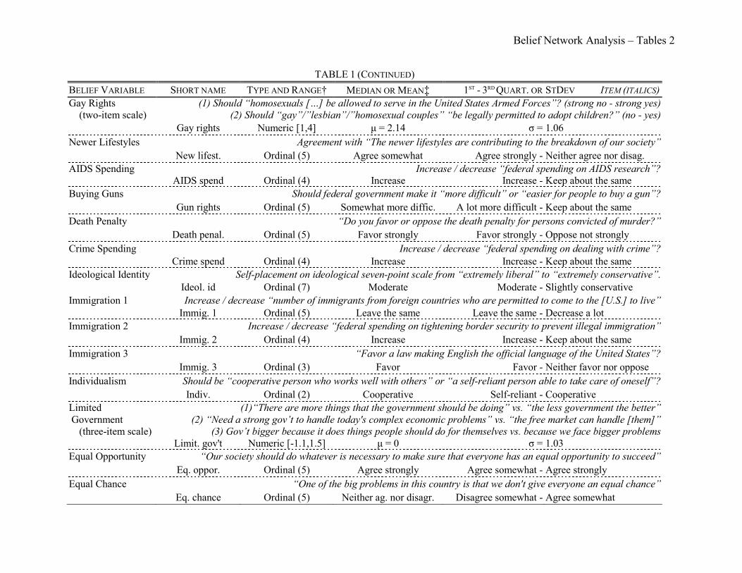
Belief Network Analysis – Tables 2
TABLE 1 (CONTINUED)
BELIEF VARIABLE SHORT NAME TYPE AND RANGE† MEDIAN OR MEAN‡ 1ST - 3RD QUART. OR STDEV ITEM (ITALICS) Gay Rights (1) Should “homosexuals […] be allowed to serve in the United States Armed Forces”? (strong no - strong yes) (two-item scale) (2) Should “gay”/”lesbian”/”homosexual couples” “be legally permitted to adopt children?” (no - yes) Gay rights Numeric [1,4] μ = 2.14 σ = 1.06
Newer Lifestyles Agreement with “The newer lifestyles are contributing to the breakdown of our society”
New lifest. Ordinal (5) Agree somewhat Agree strongly - Neither agree nor disag.
AIDS Spending Increase / decrease “federal spending on AIDS research”?
AIDS spend Ordinal (4) Increase Increase - Keep about the same
Buying Guns Should federal government make it “more difficult” or “easier for people to buy a gun”?
Gun rights Ordinal (5) Somewhat more diffic. A lot more difficult - Keep about the same
Death Penalty “Do you favor or oppose the death penalty for persons convicted of murder?”
Death penal. Ordinal (5) Favor strongly Favor strongly - Oppose not strongly
Crime Spending Increase / decrease “federal spending on dealing with crime”?
Crime spend Ordinal (4) Increase Increase - Keep about the same
Ideological Identity Self-placement on ideological seven-point scale from “extremely liberal” to “extremely conservative”.
Ideol. id Ordinal (7) Moderate Moderate - Slightly conservative
Immigration 1 Increase / decrease “number of immigrants from foreign countries who are permitted to come to the [U.S.] to live”
Immig. 1 Ordinal (5) Leave the same Leave the same - Decrease a lot
Immigration 2 Increase / decrease “federal spending on tightening border security to prevent illegal immigration”
Immig. 2 Ordinal (4) Increase Increase - Keep about the same
Immigration 3 “Favor a law making English the official language of the United States”?
Immig. 3 Ordinal (3) Favor Favor - Neither favor nor oppose
Individualism Should be “cooperative person who works well with others” or “a self-reliant person able to take care of oneself”?
Indiv. Ordinal (2) Cooperative Self-reliant - Cooperative
Limited (1)“There are more things that the government should be doing” vs. “the less government the better” Government (2) “Need a strong gov’t to handle today's complex economic problems” vs. “the free market can handle [them]” (three-item scale) (3) Gov’t bigger because it does things people should do for themselves vs. because we face bigger problems
Limit. gov't Numeric [-1.1,1.5] μ = 0 σ = 1.03
Equal Opportunity “Our society should do whatever is necessary to make sure that everyone has an equal opportunity to succeed”
Eq. oppor. Ordinal (5) Agree strongly Agree somewhat - Agree strongly
Equal Chance “One of the big problems in this country is that we don't give everyone an equal chance”
Eq. chance Ordinal (5) Neither ag. nor disagr. Disagree somewhat - Agree somewhat

Belief Network Analysis – Tables 3
TABLE 1 (CONTINUED)
BELIEF VARIABLE SHORT NAME TYPE AND RANGE† MEDIAN OR MEAN‡ 1ST - 3RD QUART. OR STDEV ITEM (ITALICS)
Inequality Agreement with “It is not really that big a problem if some people have more of a chance in life than others”
Ineq. Ordinal (5) Disagree somewhat Agree somewhat - Disagree somewhat
Parenting 1 “Please tell me which one you think is more important for a child to have: independence, or respect for elders?”
Parent. 1 Ordinal (3) Respect for elders Both - Respect for elders
Parenting 2 “Please tell me which one you think is more important for a child to have: curiosity, or good manners?”
Parent. 2 Ordinal (3) Good manners Curiosity - Good manners
Parenting 3 “Please tell me which one you think is more important for a child: being considerate, or well behaved?”
Parent. 3 Ordinal (3) Considerate Considerate - Well behaved
Party Identity Self-placement on party-identification seven point scale from “Strong Democrat” to “Strong Republican”
Party id Ordinal (7) Independent Weak Democrat - Weak Republican
Anti-Black Racism Rate blacks from (1)“hard-working” to “lazy”(2)“intelligent” to “unintelligent”(3)“trustworthy” to “untrustworthy” (three-item scale) Racism Numeric [-2.5,2.7] μ = 0 σ = 0.9
Gender Equality Men and women should “have equal roles” or “a woman’s place is in the home.”
Gender equal. Ordinal (5) Feel strongly: equal Feel strongly: equal - Feel not strongly: equal
Religiosity “Do you consider religion to be an important part of your life, or not?”
Relig. Ordinal (2) Important Important - Important
Surplus Taxes Approve / disapprove : “most of the expected federal budget surplus should be used to cut taxes”
Taxes Ordinal (2) Approve Approve - Disapprove
Tolerance Should be “tolerant of people who choose to live according to their own moral standards” even if different from ours
Toler. Ordinal (5) Agree somewhat Agree somewhat - Neither agree nor disagr.
Welfare Recipients Feelings about “people on welfare”, from not favorable/“cold” (=0) to favorable/“warm”(=100)
Welf're recip. Numeric [0,100] μ = 51.8 σ = 20.3
Welfare Spending Increase / decrease : (1) “federal spending on welfare programs?" and (2) “federal spending on food stamps?” (two-item scale) Welf're spend Numeric [1,4] μ = 2.22 σ = 0.64
NOTE.—The “short name” column contains the abbreviations we use in the network diagrams. Numeric variables are coded so that lower values correspond to respondents providing the first response option. E.g., for Anti-Black Racism, lower values corresponds to “hard-working”, “intelligent”, and “trustworthy”; for Welfare Spending, they correspond to “increase” for both types of funding. †—Ordinal variable (with number of categories), or numeric variable with range [from, to]. ‡—For ordinals, these columns show median and the 1st and 3rd quartile values. For numerics, they show mean and standard deviation.

Belief Network Analysis – Tables 4
TABLE 2 CENTRALITY OF NODES IN BELIEF NETWORK FROM FULL 2000 ANES SAMPLE
ATTITUDE
BETWEENNESS CENTRALITY
Original sample Bootstrapped (1000 row resamples)
Absolute Relative (mean & 95% CI) Absolute (mean)
Ideological Identity 0.352
0.319
Limited Government 0.119 0.105
Gay Rights 0.104 0.082
Equal Rights 1 0.074 0.076
Welfare Spending 0.089 0.065
Parenting 2 0.070 0.061
Party Identity 0.065 0.048
Biblical Literalism 0.020 0.050
Environmentalism 3 0.023 0.041
Environmentalism 1 0.046 0.039
Immigration 2 0.035 0.037
Immigration 3 0.036 0.037
Abortion Legal 0.030 0.038
Affirmative Action 0.024 0.032
Immigration 1 0.024 0.029
Equal Rights 2 0.023 0.026
Newer Lifestyles 0.016 0.017
Buying Guns 0.008 0.016
Religiosity 0.011 0.017
Foreign Aid 0.007 0.011
Equal Chance 0.008 0.009
Moral Relativism 0.005 0.010
Welfare Recipients 0.024 0.015
Equal Treatment 0.004 0.006
Military Spending 0.003 0.006
Crime Spending 0.004 0.005
Tolerance 0.001 0.004
AIDS Spending 0.003 0.005
Parenting 1 0 0.004
Equal Opportunity 0 0.004
Abortion for Teens 0 0.003
Environmentalism 2 0 0.002
Death Penalty 0 0.001
Military 0 0.001
Surplus Taxes 0 0.001
Inequality 0.001 0.001
Gender Equality 0 0.001
Parenting 3 0 0
Individualism 0 0
Anti-Black Racism 0 0

Belief Network Analysis – Tables 5
TABLE 3 STABILITY TO CHANGES IN VARIABLE SET: BETWEENNESS CENTRALITY IN 1000 COLUMN RESAMPLES
ATTITUDE
IDEOLOGICAL ID. RETAINED IDEOLOGICAL ID. DROPPED
Relative (mean and 95% CI)
Absolute (mean)
Relative (mean and 95% CI)
Absolute (mean)
Ideological Identity
0.388
—
Limited Government 0.153 0.137
Gay Rights 0.114 0.185
Welfare Spending 0.089 0.067
Equal Rights 1 0.090 0.218
Party Identity 0.078 0.111
Parenting 2 0.070 0.089
Environmentalism 1 0.047 0.040
Immigration 3 0.049 0.052
Abortion Legal 0.047 0.036
Environmentalism 3 0.046 0.067
Biblical Literalism 0.054 0.076
Equal Rights 2 0.035 0.041
Immigration 2 0.037 0.051
Affirmative Action 0.037 0.043
Immigration 1 0.030 0.049
Newer Lifestyles 0.027 0.057
Welfare Recipients 0.021 0.015
Buying Guns 0.018 0.046
Religiosity 0.010 0.028
Foreign Aid 0.011 0.015
Equal Chance 0.008 0.010
Moral Relativism 0.007 0.061
Equal Treatment 0.006 0.016
Crime Spending 0.005 0.006
AIDS Spending 0.006 0.009
Military Spending 0.003 0.030
Tolerance 0.002 0.017
Death Penalty 0.002 0.003
Equal Opportunity 0.001 0.002
Inequality 0.001 0.002
Parenting 1 0.001 0.001
Gender Equality 0 0.010
Environmentalism 2 0 0.002
Anti-Black Racism 0 0.000
Individualism 0 0.000
Military 0 0.004
Abortion for Teens 0 0.004
Surplus Taxes 0 0.003
Parenting 3 0 0

Belief Network Analysis – Tables 6
TABLE 4 SIGNIFICANT CORRELATIONS BETWEEN PAIRS OF ATTITUDES WHICH HAVE OPPOSITE SIGNS
WITHIN DIFFERENT SUBGROUPS (PERCENTAGE)
DEMOGRAPHIC SUBGROUPS (WITH GROUP SIZE)
COR’S WITH
p < 0.05
% OPPOSITE
1 2 3 4 5
Gender:
1. Male (671) ……………………… 649 — 0.4
2. Female (872) …………………… 587 0.4 — Class (self-identified) †:
1. Working class (699) …………... 582 — 1.3 2. Middle class (844) ……………… 639 1.3 — Parents foreign-born:
1. Parents Foreign-born (229) …….. 449 — 1.0 2. Not foreign-born (1310) ………... 663 1.0 — Number of children:
1. One or more children (1124) .…. 628 — 0.2 2. No children (403) ………………. 577 0.2 — Black:
1. Black (159) .……………………. 226 — 10.5 2. Not Black (1344) ………………. 683 10.5 — Hispanic:
1. Hispanic (101) …………………. 243 — 2.6 2. Not Hispanic (1432) ……………. 676 2.6 — Age group:
1. Under 40 (545) …………………. 577 — 0 1.4 2. 40 to 55 (491) …...……………… 589 0 — 1.3 3. Over 55 (499) …………………... 517 1.4 1.3 — Education:
1. High School or below (578) ……. 464 — 1.8 4.0 2. Associate or some college (467) .. 561 1.8 — 0.2 3. Bachelor’s or above (494) ……. 636 4.0 0.2 — Income:
1. Under $35,000 / year (513) ……. 510 — 0.5 1.4 2. $35,000 to $65,000 / year (385) .. 586 0.5 — 0.4 3. Over $65,000 / year (408) ……… 576 1.4 0.4 — South-Eastern United States:
1. Southern (550) ………………… 584 — 0.4 2. Not Southern (993) .……………. 640 0.4 —

Belief Network Analysis – Tables 7
TABLE 4 (CONTINUED)
DEMOGRAPHIC SUBGROUPS (WITH GROUP SIZE)
COR’S WITH
P
<0.05
% OPPOSITE SIGNS IF COMPARED TO
SUBGROUP NUMBER
1 2 3 4 5
Religion:
1. Catholic (396) ………………. 410 — 1.1 1.4 1.9 2. Mainline Protestant (420) …… 574 1.1 — 2.0 0.8 3. Other Protestant (287) ………. 423 1.4 2.0 — 2.5 4. Other Religion or none (323) .. 588 1.9 0.8 2.5 — Occupational category:
1. Manager (203) …………………. 445 — 0.5 0.3 0 1.4
2. Professional (326) …………... 587 0.5 — 0.5 0.5 2.4
3. Routine non-manual (354) …… 474 0.3 0.5 — 0.3 0.9
4. Skilled or semi-skilled (241) …. 435 0 0.5 0.3 — 1.6
5. Unskilled or farm (276) ………. 440 1.4 2.4 0.9 1.6 —
Type of place:
1. Larger city (282) ……………… 436 — 1.5 1.3 1.6 2. Rural area (431) ……………… 488 1.5 — 1.2 1.8 3. Town or smaller city (507) …… 592 1.3 1.2 — 0.2 4. Suburb (310) ………………….. 569 1.6 1.8 0.2 — Church Attendance:
1. Attends Church (1057) 641 — 0.6
2. Does Not Attend Church (478) 604 0.6 —
Cross-Pressures:
1. Pressures aligned (471) 591 — 0 1.6
2. Neither (385) 586 0 — 0.9
3. Pressures crossed (448) 499 1.6 0.9 —
Political knowledge:
1. Low (398) ……………………… 372 — 4.2 12.6 2. Medium (667) …………………. 543 4.2 — 1.6 3. High (473) .……………………. 700 12.6 1.6 —
NOTE.—Each category is compared to each other category within the same demographic dimensions. The column numbers (1 – 5) index the categories in the current dimension (E.g., for the categories within Religion, subgroup number 1 is Catholics, 2 is mainline Protestants, etc.) The counts of statistically significant correlations are out of 780 possible. See Appendix E for detailed descriptions of the variables.
† Identification with other classes is rare. 97% of respondents either “thought of” themselves as middle or working class, or identified with one of the two when prompted to do so explicitly.

Belief Network Analysis – Tables 8
TABLE 5 BELIEF CENTRALITIES FOR DIFFERENT SUBPOPULATIONS
ATTITUDE RELATIVE BETWEENNESS CENTRALITY (MEAN AND 95% CI)
High Information Respondents
Low Information Respondents
African American Respondents
Ideological Identity
Immigration 3
Welfare Spending
Equal Rights 2
Surplus Taxes
Environmentalism 1
Abortion Legal
Equal Rights 1
Limited Government
Parenting 2
Biblical Literalism
Immigration 2
Gay Rights
Abortion for Teens
Buying Guns
Affirmative Action
Party Identity
Environmentalism 3
Newer Lifestyles
Welfare Recipients
Tolerance
Military Spending
Parenting 1
Immigration 1
Religiosity
Individualism
Foreign Aid
Equal Chance
Moral Relativism
Death Penalty
AIDS Spending
Environmentalism 2
Parenting 3
Military
Gender Equality
Equal Opportunity
Inequality
Equal Treatment
Crime Spending
Anti-Black Racism
NOTE.—Each of the three sets of betweenness estimates is based on 1000 row-wise bootstraps.

Belief Network Analysis – Tables 9
APPENDIX TABLE D1 BETWEENNESS CENTRALITIES FOR ALTERNATE SELECTIONS OF BELIEFS
RELATIVE BETWEENNESS CENTRALITY (MEAN AND 95% CI)
ATTITUDE No Ideological Id. No Party Id. No Broad Stances
Ideological Identity
Equal Rights 1
Gay Rights
Limited Government
Party Identity
Parenting 2
Biblical Literalism
Environmentalism 3
Welfare Spending
Immigration 2
Moral Relativism
Immigration 1
Affirmative Action
Immigration 3
Environmentalism 1
Buying Guns
Newer Lifestyles
Abortion Legal
Equal Rights 2
Religiosity
Military Spending
Foreign Aid
Welfare Recipients
Tolerance
Equal Treatment
AIDS Spending
Equal Chance
Abortion for Teens
Parenting 1
Separate Spheres
Crime Spending
Equal Opportunity
Surplus Taxes
Environmentalism 2
Military
Death Penalty
Inequality
Parenting 3
Individualism
Anti-Black Racism
NOTE.—Each of the three sets of betweenness estimates is based on 1000 row-wise bootstraps.

Belief Network Analysis – Tables 10
APPENDIX TABLE D2
BETWEENNESS CENTRALITIES FOR ALTERNATE VARIABLE FORMATS
ATTITUDE 7-CATEGORY PARENTING 3-CATEGORY IDEOLOGY
Relative(Á and 95% CI) Abs. Relative(Á and 95% CI) Abs.
Ideological Identity (7)†
0.32
Ideological Identity (3) 0.34
Limited Government 0.11 0.11
Equal Rights 1 0.08 0.08
Gay Rights 0.07 0.07
Welfare Spending 0.07 0.07
Parenting 2 0.06
Party Identity 0.05 0.06
Biblical Literalism 0.03 0.06
Environmentalism 3 0.05 0.04
Environmentalism 1 0.04 0.04
Immigration 2 0.04 0.04
Affirmative Action 0.04 0.03
Immigration 3 0.04 0.03
Immigration 1 0.02 0.03
Abortion Legal 0.03 0.03
Equal Rights 2 0.03 0.02
Religiosity 0.01 0.02
Buying Guns 0.02 0.02
Welfare Recipients 0.02 0.02
Newer Lifestyles 0.02 0.01
Foreign Aid 0.01 0.01
Moral Relativism 0.01 0.01
Equal Chance 0.01 0.01
Military Spending 0.01 0.01
Equal Treatment 0.01 0.01
AIDS Spending 0.01 0.01
Parenting 1 0.00
Crime Spending 0.00 0.00
Tolerance 0.00 0.00
Equal Opportunity 0.00 0.00
Parenting (7) 0.00
Abortion for Teens 0.00 0.00
Environmentalism 2 0.00 0.00
Death Penalty 0.00 0.00
Inequality 0.00 0.00
Surplus Taxes 0.00 0.00
Military 0.00 0.00
Separate Spheres 0.00 0.00
Parenting 3 0.00
Individualism 0.00 0.00
Anti-Black Racism 0.00 0.00
NOTE.—Each of the three sets of betweenness estimates is based on 1000 row-wise bootstraps.
†—The parentheticals (7) and (3) indicate the number of categories in the variable.

Belief Network Analysis – Figures 1
FIGURES
FIG. 1.—Belief network at different stages.
(1) After 1st generation
(2) After 2nd generation
(3) Snippet of a large belief
network.

Belief Network Analysis – Figures 2
FIG. 2.— Correlation network for the full population sample (see Table 1 for full node names).
Tie strength +*�!+ = ��� ��, �!" is represented by thickness and boldness (see inset).
Correlations below |�| = 0.15 are not depicted. The force-directed layout places strongly connected nodes closer together, and weakly connected and unconnected nodes further apart.

Belief Network Analysis – Figures 3
FIG. 3.— Degree of organization in belief networks of 44 demographic subgroups. Filled circles indicate networks where the most central node was ideological identity.

Belief Network Analysis – Figures 4
FIG. 4.— Network centralization by centrality of ideological identity in 44 demographic subgroups, with line of best fit.

Belief Network Analysis – Figures 5
FIG. 5. Correlation network for the high information subsample (see Table 1 for full node names).
Tie strength is represented by thickness and boldness (see inset). Correlations below |�| = 0.15 are not depicted. Force-directed layout.

Belief Network Analysis – Figures 6
FIG. 6. Correlation network for the low information subsample (see Table 1 for full node names).
Tie strength is represented by thickness and boldness (see inset). Correlations below |�| = 0.15 are not depicted. Force-directed layout.

Belief Network Analysis – Figures 7
APPENDIX FIGURES
FIG. A1.—There are three possible relative locations for stranger ties *(�, ?) and *(�, |) in a path Λ({, z): (i) the two ties could be
immediately adjacent, i.e., ? = � (ii) � could be a descendant of ? (iii) � could be an ancestor of ?. Solid lines indicate ties, whereas dashed lines indicate ancestry. Possible omitted network segments. Note that the proof does not require f and g to be strangers.
(i) (ii) (iii)

Belief Network Analysis – Figures 8
FIG. A2.—Geodesics between stranger nodes can follow one of two topologies: (i) central and (ii) non-central.
(i) (ii)