Progressive Approach to Relational Entity Resolution

Yasser Altowim Dmitri V. Kalashnikov Sharad Mehrotra

Department of Computer ScienceUniversity of California, Irvine

ABSTRACTThis paper proposes a progressive approach to entity reso-lution (ER) that allows users to explore a trade-off betweenthe resolution cost and the achieved quality of the resolveddata. In particular, our approach aims to produce the high-est quality result given a constraint on the resolution bud-get, specified by the user. Our proposed method monitorsand dynamically reassesses the resolution progress to deter-mine which parts of the data should be resolved next andhow they should be resolved. The comprehensive empiricalevaluation of the proposed approach demonstrates its sig-nificant advantage in terms of efficiency over the traditionalER techniques for the given problem settings.

1. INTRODUCTIONEntity resolution (ER) is a well-known data quality chal-

lenge that arises when real-world objects are referred to us-ing entities or descriptions that are not always unique iden-tifier of the objects [3, 5, 8, 23, 24]. The task of ER is todetermine which entities refer to the same real-world ob-ject. A typical ER process consists of two phases: (a) apruning phase that uses strategies, such as blocking [14,18],to partition the dataset into a set of (possibly overlapping)blocks such that entities in different blocks are unlikely toco-refer, and (b) a (potentially expensive) resolution phasethat determines duplicate entities within each block.

Traditionally, the ER problem has been studied in thecontext of data warehousing as an offline pre-processing stepprior to data analysis. Such an offline strategy is not suit-able for many emerging applications that require (near) real-time analysis, especially if it involves big, fast, or streamingdata [22]. To address the needs of such applications, in-stead of cleaning data fully, a preferred approach is to cleandata progressively in a pay-as-you-go fashion, while contin-ually/periodically analyzing the partially cleaned data toprogressively compute better analysis results.

Such a progressive approach is a new paradigm for entityresolution. It aims to identify and resolve as many dupli-

This work is licensed under the Creative Commons Attribution-NonCommercial-NoDerivs 3.0 Unported License. To view a copy of this li-cense, visit http://creativecommons.org/licenses/by-nc-nd/3.0/. Obtain per-mission prior to any use beyond those covered by the license. Contactcopyright holder by emailing info@vldb.org. Articles from this volumewere invited to present their results at the 40th International Conference onVery Large Data Bases, September 1st - 5th 2014, Hangzhou, China.Proceedings of the VLDB Endowment, Vol. 7, No. 11Copyright 2014 VLDB Endowment 2150-8097/14/07.

cate entities in the dataset as possible while trying to avoidresolving non-duplicate entities. For this purpose, a progres-sive ER approach prioritizes/ranks which parts of the datato resolve first in order to maximize the number of resolvedduplicate entities.

The work on progressive data cleaning [9, 15, 22] is at anearly stage with [22] being the first to explore it in the con-text of ER. In [22], the authors focus on maximizing thequality of the cleaned data given a user-defined resolutionbudget (e.g., 5 minutes). They propose several concreteways of constructing resolution “hints” that can be thenused by a variety of existing ER algorithms as a guidancefor which entities to resolve first.

While [22] addresses the problem of progressive ER, theirsolution considers resolving only a single entity-set contain-ing duplicates. In this paper, we study the problem inthe case of relational ER [6, 11, 12, 23]. In relational ER,the dataset consists of multiple entity-sets and relationshipsamong them. In such a dataset, a resolution of some entitiesmight influence the resolution of other entities. For exam-ple, deciding that two research papers are the same maytrigger the fact that their venues are also the same. Priorresearch [6, 11, 12] has shown that such decision propaga-tion via relationships can significantly improve data qualityin datasets where such relationships can be specified. Ourchallenge in this paper is to make such ER techniques thatuse decision propagation (e.g., [11,12]) progressive.

The dependency between resolution decisions in relationalER influences our design in two ways. First, as more partsof the dataset are resolved, new information about which en-tities tend to co-refer becomes available. Thus, an adaptivestrategy that dynamically revises its ranking is more suitedfor progressive relational ER. Second, unlike a single entity-set situation where there may not be a strong reason to pre-fer one block over another to resolve first, such a block-levelprioritization is significantly more important when resolvingrelational datasets. For instance, resolving a block that in-fluences many other parts of the dataset might significantlyimprove the performance of a progressive approach.

Motivated by the two factors, we develop an adaptive pro-gressive approach to relational ER that aims to generate ahigh-quality result using a limited resolution budget. Toachieve adaptivity, our approach continually reassesses howto solve two key challenges: “which parts of the dataset toresolve next?” and “how to resolve them?”. For that, itdivides the resolution process into several resolution win-dows and analyzes the resolution progress at the beginningof each window to generate a resolution plan for the current

Block P Id Title Abstract Keywords Authors Venue

P1p1 Transaction Support in Read Optimized and ... ... {File System, Transactions} {a1, a2} u1

p3 Transaction Support in Read Optimized and ... ... {File System, Transactions} {a3, a4} u3

P2p2 Read Optimized File System Designs: A performance ... ... {File System, Database} {a1} u2

p4 Berkeley DB: A Retrospective ... {File System, Database} {a3} u4

(a) Entity-set Papers.

Block A Id Name Email Papers

A1a1 Margo Seltzer margo@harvard.edu {p1, p2}a3 Margo I. Seltzer seltzer@gmail.com {p3, p4}

A2a2 Michael Stonebraker stonebraker@mit.edu {p1}a4 M. Stonebraker stonebraker@ucb.edu {p3}

(b) Entity-set Authors.

Block V Id Name Papers

U1u1 Very Large Data Bases {p1}u3 VLDB {p3}

U2u2 ICDE Conference {p2}u4 IEEE Data Eng. Bull {p4}

(c) Entity-set Venues.Table 1: Toy Publication Dataset.

window. A resolution plan specifies which blocks and whichentity pairs within blocks need to be resolved during the planexecution phase of that window. Furthermore, our approachassociates with each identified pair of entities a workflow –the order in which to apply the similarity functions on thepair. Such an order plays a significant role in reducing theoverall cost because applying the first few functions in thisorder might be sufficient to resolve the pair.

While an adaptive approach may help quickly identify du-plicate pairs in the dataset, such a technique must be imple-mented carefully so that the benefits obtained are not over-shadowed by the associated overheads of adaptation. Weachieve this by designing efficient algorithms, appropriatedata structures, and statistics gathering methods that donot impose high overheads. Our results in Section 7 showhow our approach can generate a high-quality result usinga limited amount of resolution budget.

Overall, the main contributions of this paper are:

• We propose an adaptive progressive approach to the prob-lem of relational entity resolution (Section 3).

• We present a benefit and a cost models for generating aresolution plan (Section 4).

• We show that the problem of generating a resolution planis NP-hard, and thus propose an efficient approximatesolution that performs well in practice (Section 5).

• We define the concept of the contribution of similarityfunctions, and then show how the cost and contributionof multiple similarity functions can be exploited to reducethe resolution cost (Section 6).

• We experimentally evaluate our approach using publica-tion and synthetic datasets and demonstrate the efficiencyof the proposed solution (Section 7).

2. NOTATION AND PROBLEM DEFINITIONIn the following subsections, we first develop notation, and

then define the problem of progressive ER.

2.1 Relational DatasetLet D be a relational dataset that contains a number of

entity-sets D = {R,S, T, . . . }. Each entity-set R containsa set of entities of the same type R = {r1, r2, . . . , r|R|}.Entity-set R is considered dirty if at least two of its entitiesri and rj represent the same real-world object, and henceri and rj are duplicate. We denote the attributes in R asR.A = {R.a1, R.a2, . . . , R.a|R.A|}. An attribute R.a can bea reference attribute, i.e., its values are references to otherentities in other entity-sets.

Table 1 shows an example of a relational publication dataset.It contains three entity-sets: papers P , authors A, andvenues U . Entity-set P contains one duplicate pair 〈p1, p3〉.Entity-set A contains two duplicate pairs 〈a1, a3〉 and 〈a2,a4〉, and entity-set U contains one duplicate pair 〈u1, u3〉.

2.2 Standard Phases of ERA typical ER process consists of several standard phases

of data transformations. We list these phases below andexplain how we instantiate some of them.

• Blocking [14,18] that partitions each entity-set into (pos-sibly overlapping) smaller blocks such that entities in dif-ferent blocks are unlikely to co-refer. The goal of block-ing is to reduce the (often quadratic) process of applyingER on the entire entity-set to that of applying ER onthe small blocks. In our approach, we also assume thateach entity-set R ∈ D is partitioned into a set of blocksBR = {R1, R2, . . . , R|BR|}

1.

• Problem Representation that maps the data into an inter-nal data representation of the ER algorithm. We repre-sent our problem as a graph, as detailed in Section 2.3.

• Similarity Computation that computes the similarity be-tween entities in the same block. This phase is oftencomputationally expensive as it might require resolvingO(n2) pairs of entities per cleaning block of size n. Eachresolution might apply several similarity functions on thepair of entities. A high-quality similarity function can beexpensive in general as it may require invoking compute-intensive algorithms, consulting external data sources, on-tology matching, and/or seeking human input throughcrowdsourcing [19,21].

Correspondingly, in our approach, each entity-set R ∈D is associated with multiple similarity functions FR ={fR

1 , fR2 , . . . , f

R|FR|}. These similarity functions are as-

sumed to be “black-boxes” [5,8]. Each function fRi takes

as input a pair of entities 〈rj , rk〉 and returns a normalizedsimilarity score for rj and rk – a value from the [0, 1] inter-val. This score is computed by fR

i by analyzing the valuesof rj and rk in some of the non-reference attributes A(fR

i )of R. For instance, function fP

1 in Table 2 is defined onthe Title attribute of entity-set P , i.e., A(fP

1 ) = {Title}.Given two titles of two papers, fP

1 returns their title sim-ilarity using the standard Edit-Distance algorithm.

Each similarity function fRi in turn is associated with a

cost cRi , which represents an average cost of applying fRi

1For clarity, we will present the paper as if blocks do not overlap.

Extending our approach to overlapping blocks is straightforward, see[1] for details. In fact, our experiments on the publication datasetuse overlapping blocks.

Function Attributes Similarity Algorithm

fP1 P .Title Edit Distance

fP2 P .Abstract TF.IDF

fP3 P .Keywords Edit Distance

fA1 A.Name Edit Distance

fA2 A.Email JaroWinkler Distance

fU1 U .Name Edit Distance

Table 2: Description of the Similarity Functions.

on a pair of entities. Our approach is agnostic to theway this cost is set. For instance, we set it as the averageexecution time of fR

i learned from the dataset. But it alsocould be a unit-based cost set by the domain analysts, etc.

In the case where multiple similarity functions are used onan entity-set R, there could be a resolve function whosetask is to combine the values of these multiple functionsinto a single value. We explain our resolve functions inSection 2.3.

• Clustering that groups duplicate entities into clusters basedon the values computed by similarity/resolve functionssuch that each cluster represents one real-world object,and each real-world object is represented by one clus-ter [5, 12,19].

• Merging that combines entities of each individual clusterinto a single representative entity that will represent thecluster to the end-user or application in the final result.

2.3 Relational Entity ResolutionThe task of relational ER is to resolve all entity-sets of a

given relational dataset. In addition to exploiting the sim-ilarity between entity attributes as in traditional ER, rela-tional ER also utilizes the relationships among the entity-sets to further improve the quality of the result [6, 12].

To illustrate, consider the paper pair 〈p1, p3〉 in Table 1.By applying the similarity functions on it, we can decidethat p1 and p3 co-refer. This decision can be propagated tothe pair of their venues 〈u1, u3〉. Based on that, we mightthen decide that 〈u1, u3〉 co-refer, which might not have beenachievable had we relied only on the similarity function ofU since their venue names are spelled very differently.

Influence. In relational ER, there is an influence LR→S

from entity-set R to S if resolving some pairs from R caninfluence (provide evidence) for resolving some pairs from S.For example, the dataset in Table 1 has an influence LP→U

since if two papers are the same, their venues are likely tobe the same as well. We denote the set of influences of Das L(D). For instance, if D corresponds to the dataset inTable 1, then L(D) = {LP→A, LP→U , LA→P , LU→P }.

In an influence LR→S , R is called the influencing entity-set and S is the dependent entity-set. Inf(R) is the set ofall LR→X influences for any X, and Dep(S) is the set ofall LX→S influences for any X. In the example in Table 1,Inf(P ) = {LP→A, LP→U} and Dep(P ) = {LA→P , LU→P }.ER Graph. To capture decision propagation, it is oftenconvenient to model the problem as a graph [11,12].

Graph G = (V,E) is a directed graph, where V is a setof nodes and E is a set of edges. A node vi is created fora pair of entities 〈rj , rk〉 iff there exists at least one blockRl that contains both rj and rk. The node vi representsthe fact that 〈rj , rk〉 could be the same, which needs to befurther checked. An edge is created from node vi = 〈rj , rk〉

u2, u4

p1, p3

p2, p4a1, a3

a2, a4 u1, u3

v1 v3 v5

v2 v4 v6

Figure 1: Graph Representation.

to node vl = 〈sm, sn〉 iff there exits an influence LR→S andthe resolution of vi can influence the resolution of vl.

Figure 1 shows the graph corresponding to the publica-tion dataset in Table 1. Node v3 represents the possibilitythat entities p2 and p4 could be the same. An edge from v1to v3 indicates that the resolution of v1 influences the reso-lution decision of v3 via LA→P . Therefore, node v3 has oneinfluencing node v1 via LA→P . Node v1 has two dependentnodes v3 and v4 via LA→P .

Having defined the graph, we now can develop some use-ful auxiliary notation that relates this graph to blocks. LetBK(vi) be the function that, given a node vi, returns theblock that contains both of the two entities that vi repre-sents. Let V (Ri) be the set of all nodes of block Ri. Note

that V (R) =⋃|BR|

i=1 V (Ri).From the graph representation point of view, the task of

relational ER can be viewed as that of determining whethereach node vi ∈ V represents a duplicate pair of entities ornot. That resolution decision is based on the outputs of ap-plying the similarity functions of R on vi and the resolutiondecisions of vi’s influencing nodes. Such a decision can bemade after the application of a “black-box” resolve functionon the node vi.

Resolve Functions. Each entity-set R is associated witha resolve function <R. When <R is applied on a node vi ∈V (R), it outputs a pair of confidence values: a similarityvalue simi ∈ [0, 1] and a dissimilarity value disi ∈ [0, 1] thatrepresent the collected evidence that the two entities in vico-refer and are different respectively. Initially, both valuesare set to 0. After calling <R on vi, the node vi is markedas duplicate if simi = 1, as distinct if disi = 1, or asuncertain otherwise. A node is said to be certain if it ismarked as either duplicate, or distinct. We will denotethe set of duplicate nodes of block Ri as V +(Ri) and ofentity-set R as V +(R).

As common, our resolve function <R takes as input afeature vector fi that corresponds to node vi = 〈rj , rk〉. Thevector fi is of size |fi| = |FR| + |Dep(R)| and encodes initself two types of features: (1) the outputs of applying thesimilarity functions of R on the pair 〈rj , rk〉 and (2) the setsof confidence value pairs of all nodes that influence vi, wherea set is included per each influence in Dep(R). For example,consider node v3 in Figure 1. Suppose that the outputs ofapplying the functions fP

1 , fP2 , and fP

3 on v3 are 0.2, 0.1,and 0.9 respectively, and that 〈sim1, dis1〉 = 〈1.0, 0.0〉 and〈sim5, dis5〉 = 〈0.0, 1.0〉. The input to <P is therefore thefeature vector f3 = (0.2, 0.1, 0.9, {〈1.0, 0.0〉}, {〈0.0, 1.0〉}).

The above discussed model of resolve functions is genericto capture a wide range of possible implementations of re-solve functions. In our experiments on the publication dataset,we implement the resolve function as a binary Naive Bayesclassifier that classifies each input feature vector into eitherof the two classes “duplicate” or “distinct” and returns theprobability that the input vector belongs to each class.

2.4 Progressive Entity ResolutionGiven a relational dataset D along with a set of similarity

functions FR and a resolve function <R for each entity-setR ∈ D, and a resolution budget BG, our goal is to develop aprogressive ER approach that produces a high quality resultby using no more than BG units of cost.

Developing an optimal progressive approach is infeasiblein practice as it would require an “oracle” that knows inadvance the set of pairs that, when resolved, will have thehighest influence on the quality of the result. Thus, our goaltranslates into finding a good strategy that best utilizes thegiven budget by saving cost at two different levels. First,our strategy should clean only the parts of the dataset thathave higher influence on the quality of the result. That is,it should aim to find and resolve as many duplicate pairsas possible, because the more duplicate pairs it correctlyidentifies, the higher the quality of the result is expected tobe2. Second, it should resolve those identified pairs with theleast amount of cost.

3. OVERVIEW OF OUR APPROACHOur progressive ER approach resolves the dataset D by

incrementally constructing the ER graph and resolving itsnodes. At any instance of time, the approach maintains apartially constructed ER graph Gp = (V p, Ep) which is asubgraph of the ER graph G(V,E) that corresponds to theentire dataset D; i.e., V p ⊆ V and Ep ⊆ E. We refer tothe nodes and edges in Gp as instantiated nodes and edgesof G. The instantiated nodes in Gp are further separatedinto resolved nodes, denoted as RV, and unresolved nodes,denoted as UV, based of whether the approach has alreadyresolved the node (i.e., applied the similarity functions onit and then marked it as duplicate, distinct, or uncertain)or not. Figure 2 depicts an example of a graph G and apartially constructed graph Gp.

Resolution Windows. To incrementally build and resolvethe graph GP , we divide the total budget BG into severalresolution windows. Each window consists of two phases:plan generation followed by plan execution. In the plan gen-eration phase, our approach determines the activities thatshould be performed in the next W units of cost. The pa-rameter W is the duration of the plan execution phase andit is of the same cost unit as BG; e.g., if the unit of cost isthe execution time, then BG could be, say, 1 hour and Wcould be 3 minutes. Generating a plan for a window involvesidentifying a set of nodes to be resolved during the plan exe-cution phase of that window. This set is chosen from the setof candidate nodes CV = V −RV (which are the nodes thathave not been resolved yet) based on a trade-off between thebenefit and cost of resolving these nodes.

Before we explain the plan generation and execution phases,let us first describe how our approach incrementally buildsthe graph Gp. If a node vi is chosen to be resolved and it isnot currently instantiated in Gp, then it is first instantiated.Instantiation is performed in unit of blocks; that is, if a nodevi needs to be instantiated in a window, then we instantiatethe entire block BK(vi).

Block Instantiation. The process of instantiating a blockRi involves reading all entities of Ri, creating a node for

2We operate under the condition that most of the pairs in the dataset

are distinct [22], which is often the case in real-world datasets.

v9

v6

v1

v2

v7

v10

v11v3

v8

Unresolved Node Duplicate Node Distinct Node

R1 T1

S2

S1

R2

v4

Instantiated Block Uninstantiated Block

v5

v12

T2

Gp

Figure 2: A Partially Constructed Graph Gp.

each pair of entities of Ri, and adding edges based on de-pendency. In addition, we also determine, for each entityin Ri, the set of its dependent entities via each influenceLR→S ∈ Inf(R), and the blocks to which those dependententities belong. For example, when instantiating the blockA2 in Table 1, we determine that entity p1 depends uponentity a2 via LA→P , entity p3 depends upon entity a4 viaLA→P , and entities p1 and p3 belong to the block P1. Suchinformation is essential to create the outgoing edges fromthe nodes in V (Ri) to their dependent instantiated nodes,and to infer their uninstantiated dependent nodes which canbe useful in determining which nodes to resolve in the nextwindows. Instantiating at the granularity of a block helpsbring significant savings since the cost of reading the nodes(possibly from disk/storage) is only incurred once per block.Thus, prior to the beginning of a window, the blocks in Dcan be classified as instantiated blocks, which are the blocksthat have been instantiated in previous windows, and unin-stantiated blocks, denoted as UB.

Plan Generation. During the plan generation phase of awindow, our approach generates a resolution plan P̄ thatspecifies the set of blocks to be instantiated in the window,denoted as P̄B, and the set of nodes to be resolved in thewindow, denoted as P̄V. A resolution plan is said to bevalid only if, for every uninstantiated node vi ∈ P̄V, theblock BK(vi) ∈ P̄B. For example, suppose that the graphGp at the beginning of the current window is as depictedin Figure 2. If P̄V = {v3, v8} and P̄B does not contain S2,then the generated plan is not valid as the resolution of v8will not be applicable without instantiating S2.

Each possible resolution plan is associated with a notionof cost and benefit. The cost of a plan P̄ is the summation ofthe instantiation cost of every block in P̄B and the resolutioncost of every node in P̄V. To estimate the resolution cost ofa node vi, we need to associate a workflow with that nodewhich specifies how vi is to be resolved (explained next).The benefit of a plan P̄ measures the value of resolving thenodes in P̄V. Note that instantiating a block Ri ∈ P̄B, byitself, does not provide any benefit to the resolution processbut it may be required to ensure the validity of the plan.The benefit and cost models are presented in Section 4.

The process of plan generation starts by ensuring that ev-ery block in UB is associated with an updated instantiationcost value and every node in CV is associated with updatedresolution cost and benefit values. Then, it enumerates asmall set of alternative valid plans whose estimated cost isless than or equal to W , and chooses the plan with the high-est estimated benefit. Note that the process of generating a

plan itself consumes some cost from the budget BG. Thus,a key challenge is to generate a beneficial plan in a smallamount of cost. The process of generating a valid resolutionplan is explained in Section 5.

Plan Execution. The process of executing a plan P̄ startsby instantiating the blocks in P̄B, and then iterates over allthe nodes in P̄V to resolve them3. One naive strategy forresolving a node vi ∈ V (R) is to apply all the similarityfunctions of R on that node, and then call the resolve func-tion <R on vi to determine its resolution decision. However,in practice, it is often sufficient to apply a subset of thesefunctions to resolve the node to a certain decision. Thus,our approach follows a lazy resolution strategy that delaysthe application of a similarity function on a node until it isneeded. To resolve a node vi ∈ V (R) using this strategy,we apply the similarity functions of R on vi in a specificorder, referred to as the workflow of vi (the details of howworkflows are generated and associated with nodes are pre-sented in Section 6). After the application of each similarityfunction, we call the resolve function <R on vi to determineif it is certain or not. If the node is uncertain, we applythe next similarity function in the workflow on vi, and thencall <R on the node again. This process continues until thenode is certain, or there is no more similarity function toapply on the node.

After resolving all nodes in P̄V, their resolution decisionsare propagated to their dependent nodes in GP that are stilluncertain. To do so, our approach stores those dependentnodes into a set H, and then iterates over them. For eachnode vj ∈ H, our approach calls the corresponding resolvefunction on vj , and then inserts its uncertain dependentnodes into H to further propagate the decision of that node.To ensure that the propagation process terminates, we insertthose dependent nodes into H only when vj was resolved toa certain decision, or when the increase in simj or disj dueto the last application of the resolve function on vj exceedsa small constant.

Early Termination. On the completion of the budget BG,all uncertain and unresolved nodes in the graph G are de-clared to be distinct. Although there can be sophisticatedapproaches to making decisions about those nodes, such ap-proaches add to the overall computational complexity. Sinceour approach finds duplicate entities early, declaring thosenodes to be distinct is expected to perform well.

4. BENEFIT AND COST MODELSIn this section, we discuss how we estimate the benefit

and cost of a resolution plan.

4.1 Benefit ModelWe will first describe how we compute the benefit of a

node vi and then show at the end of this section how we es-timate the benefit of a plan. In relational ER, the resolutiondecision of a node vi depends upon the resolution decisionsof other nodes in the graph G. Thus, the probability ofvi to be duplicate at any instance of time can be inferredfrom the state of the graph G (i.e., which nodes have beenresolved to duplicate so far), denoted as S. Therefore, thebenefit of a node vi can be determined based on whether vi

3The actual cost of executing a plan might be different from its esti-

mated cost since we can never accurately determine the exact cost ofinstantiating a block or resolving a node.

is duplicate or not (direct benefit) and how useful declaringvi to be duplicate is in identifying more duplicate nodes inG (indirect benefit or the impact of vi). More formally, thebenefit of a node vi is defined as follows:

Benefit(vi) = P(vi|S) + P(vi|S) ∗ Imp(vi) (1)

where P(vi|S) is the probability that the node vi is du-plicate given the current state of the graph G, and Imp(vi)is the impact of vi which is defined as follows:

Imp(vi) =∑

vj∈Topvi

P(vj |Svi)−∑

vk∈Top

P(vk|S) (2)

where Svi is the state of the current graph after declar-ing vi to be duplicate, Top is a set of unresolved nodes thatcan be resolved within the remaining cost of our budget BG(i.e., the total of their resolution costs and the instantiationcosts of their blocks, if needed, is less than or equal to theremaining budget) such that the summation of their prob-ability values given S is maximized, and Topvi is a set ofunresolved nodes that can be resolved within the remainingcost of our budget minus the resolution cost of vi such thatthe summation of their probability values given Svi is max-imized. For simplicity, we will denote the value P(vi|S) asP(vi) henceforth.

Computing the exact benefit of a node vi is infeasible inpractice for two reasons. First, computing the probabilityvalue of a node given a state requires the graph G to be fullyinstantiated to infer the dependency between the nodes (incontrast, we construct G progressively), and is also equiv-alent to the belief update problem in Bayesian Networks,which is known to NP-hard [10]. Second, identifying each ofthe Top and Topvi sets can be easily proved to be NP-hardas it contains the traditional knapsack problem as a specialcase. Therefore, we use heuristics to compute Benefit(vi).The values of P(vi) and Imp(vi) are estimated as below.

Probability Estimation. We estimate the value of P(vi)using the Noisy-Or model [20] which models the interactionamong several causes on a common effect. We model thenode vi being duplicate as an effect yi that can be pro-duced by any members of a set of binary causes Xi ={xi1, xi2, . . . , xin}. These causes in our case correspond tothe direct influencing nodes of vi and the block BK(vi).That is, the probability value P(vi) is estimated based onwhich of vi’s influencing nodes are duplicate and/or on thepercentage of duplicate nodes in the block BK(vi).

Each cause xij can be either present or absent, and has a

probability P(yi|xij) of being capable of producing the ef-

fect when it is present and all other causes in Xi are absent.The Noisy-Or model assumes that the set of causes Xi areindependent of each other4, and therefore computes the con-ditional probability P(vi) = P(yi|Xi) as follows:

P(vi) = 1− (1− δ)∏

xij∈Xi

p

1− P(yi|xij)1− δ (3)

where the parameter δ is a leak value (explained later)and Xi

p is the set of present causes in Xi. If a cause xij cor-

responds to a node vk that influences vi via LS→R, then xij4One could also use a more advanced model such as the Recursive

Noisy-Or model [17] to allow for dependent causes to be used in es-timating the probability of an effect. However, such dependency be-tween causes is rarely observed in datasets and often requires signifi-cant effort to be identified.

is present only if vk was resolved to duplicate in a previouswindow, and thus we set P(yi|xij) to the value PS→R. Thisvalue refers to the probability that a node vl ∈ V (R) is du-plicate given that there exists a duplicate node vm ∈ V (S)that influences vl via LS→R, and all other causes of yl areabsent. Such a probability value can be specified by a do-main expert or learned from a training dataset. On the otherhand, if xij corresponds to the block BK(vi) = Rk, then we

set P(yi|xij) to the value |V+(Rk)|

|V ∗(Rk)|, where V ∗(Rk) is the set

of nodes of Rk that have been resolved in previous windows,but we require that xij be present only if the fraction of re-solved nodes in Rk is at least α, i.e., |V ∗(Rk)| ≥ α∗|V (Rk)|,where α is a predefined threshold. Such a requirement is notnecessary to our approach, but rather helps improve the ac-curacy of estimating the probability value of nodes.

As an example, consider the graph in Figure 2. Supposethat PR→S = 0.4 and α = 0.3. Then, X5

p consists of threecauses that correspond to the nodes v1 and v2 and the blockS1, whereas X8

p consists of one cause that corresponds to thenode v2. Therefore, P(v5) = 1−(1−0.4)∗(1−0.4)∗(1− 1

2) =

0.82 and P(v8) = 1− (1− 0.4) = 0.4.The above model states that if all influencing nodes of vi

are either distinct, uncertain, or unresolved, and the fractionof resolved nodes in BK(vi) is less than α, then the node vican not be duplicate. To overcome this limitation, the LeakyNoisy-Or model [13] allows us to assign a non-zero leakprobability value δ to P(vi). This leak value represents theprobability that vi is duplicate in the absence of all explicitlymodeled causes of yi, and it can be different for differententity-sets. For instance, the leak value δ assigned to nodesof R can be different from that assigned to nodes of S.

Impact Estimation. To estimate the value of Imp(vi),instead of considering all nodes in Top and Topvi , we restrictthe impact computation to a small subset of nodes, denotedas N (vi), and hence define the impact of vi as follows:

Imp(vi) =∑

vj∈N (vi)

[P(vj |Svi)− P(vj |S)] (4)

where the probability values in Equation 4 are computedas in Bayesian Networks (not using our approximation model(Equation 3)). Clearly, the set N (vi) should include thenodes that will be affected the most by the resolution of vi.Thus, we include in N (vi) the unresolved nodes that can bereached from vi by following at most β edges (the parameterβ is explained later).

Even after restricting the impact computation to the setN (vi) only, computing an impact value for every candidatenode vi is still infeasible for two reasons. First, computingP(vj |Svi) is in general an NP-hard problem [10]. Althoughthere are approximation algorithms for this problem [16],such algorithms are still expensive for our real-time settings.Second, identifying N (vi) might not be possible in certaincases unless the graph G is fully instantiated.

Thus, we instead compute a single estimated impact value,denoted as Imp(R), for every entity-set R and use that singlevalue as the impact value of every candidate node vi ∈ V (R).This value is computed based on statistics that we collectprior to and throughout the execution of our approach.

To estimate the value of Imp(R), we first define U(k, LR→S)as the function that computes, for k nodes of entity-set R,the estimated number of their unresolved direct dependent

Compute-Impact(R, β)1 if β = 0 then2 return 03 imp← 04 V isited← {R}5 foreach LR→S ∈ inf(R) do6 k ← U(1, LR→S) // Equation 57 〈m,V isited〉 ← Compute-Prob-Inc(R,S, k, V isited, β)8 imp← imp+m9 return imp

Compute-Prob-Inc(R,S, k, V isited, β)1 V isited← V isited ∪ {S}2 n← PR→S ∗ k3 if β − 1 = 0 then4 return 〈n, V isited〉5 foreach LS→T ∈ inf(S) s.t. T 6∈ V isited do6 k ← U(k, LS→T ) // Equation 57 〈m,V isited〉 ← Compute-Prob-Inc(S, T, k, V isited, β − 1)8 n← n+ PR→S ∗m9 return 〈n, V isited〉

Figure 3: Impact Computation.

nodes via LR→S . That is, this function estimates the num-ber of the direct dependent nodes via LR→S that will beimpacted by the resolution of the k nodes. The output ofthis function can be computed as follows:

U(k, LR→S) = dk ∗ degree(LR→S) ∗ (1− |V∗(S)||V (S)| )e (5)

where degree(LR→S) is the average number of direct de-pendent nodes that a node vi ∈ V (R) can have via LR→S .Such a value can be initially set by a domain expert orlearned from a training dataset, and can then be adjustedas our approach proceeds forward.

Now, the impact value Imp(R) can be estimated by callingthe Compute-Impact(.) function in Figure 3 with these val-ues (R, β) (the value of β is explained next). As an example,let D correspond to the dataset whose ER graph is depictedin Figure 2. Suppose that L(D) = {LR→S , LS→T }. Letus further assume that PR→S = 0.4 and PS→T = 0.5, andthat degree(LR→S) = 2 and degree(LS→T ) = 1. Assume wewant to compute the value of Imp(R) and that the value of βis 2. In this case, the value of U(1, LR→S) = 1∗2∗(1− 2

4) = 1,

and the value of U(1, LS→T ) = 1∗1∗ (1− 04) = 1. Thus, the

value of Imp(R) = PR→S ∗ U(1, LR→S) + PR→S ∗ PS→T ∗U(1, LS→T ) = 0.4 ∗ 1 + 0.4 ∗ 0.5 ∗ 1 = 0.6.

Using this model allows the impact computation to beperformed very efficiently (as we need to compute only asingle impact value for each entity-set R ∈ D) and worksvery well as we show in Section 7.

The parameter β has the same value for all entity-sets, butthat value is updated throughout the execution. Intuitively,such a value should be continually reduced to limit the im-pact computation to only the dependent nodes that have ahigh chance of being resolved in the remaining budget RM .Thus, we update the value of β at the beginning of eachwindow to

⌊γ ∗ RM

BG+ 0.5

⌋, where γ is the number of edges

in the longest non-cyclic path between any two nodes in theinfluence graph whose nodes correspond to the entity-sets inD and whose direct edges correspond to the influences L(D).For example, the influence graph of the dataset whose ERgraph is depicted in Figure 2 consists of |D| = 3 nodes (thatcorrespond to the entity-sets R, S, and T ) and two edges(R→ S and S → T ), and thus γ = 2. Decreasing the value

of β will cause the impact computation of a node vi ∈ V (R)to be restricted to only the dependent nodes of the entity-sets that are close to R in the influence graph, which are thenodes that will be affected the most by the resolution of viand thus have a high chance of being resolved later.

Plan Benefit. We measure the benefit of a plan P̄ as thesummation of the benefit of resolving each node in P̄V:

Benefit(P̄) =∑

vi∈P̄V

Benefit(vi) (6)

4.2 Cost ModelThe cost of a resolution plan P̄ is computed as follows:

Cost(P̄) =∑

Ri∈P̄B

Cins(Ri) +∑

vj∈P̄V

Cres(vj) (7)

where Cins(Ri) is the cost of instantiating the block Ri,and Cres(vj) is the cost of resolving the node vj . The costCins(Ri) typically consists of the cost of reading the blockRi, plus the cost of creating nodes for the pairs of enti-ties of Ri. The instantiation cost depends upon where theblocks are stored. In practice, blocks could be stored on alocal machine, on the cloud, or anywhere else. In Section 7,we provide a model for estimating the instantiation cost ofblocks that are stored on a local machine’s disk.

The resolution cost Cres(vj) depends upon the order inwhich the similarity functions of R are applied on the nodevj ; i.e., the workflow of vj . Associating a workflow witha node depends upon the probability of that node to beduplicate. Thus, to estimate the resolution cost of a nodevj , we first need to estimate the value of P(vj), use thatvalue to associate a workflow with vj , and then estimate thevalue of Cres(vj) based on the associated workflow. Thedetails of how the resolution cost of a node is estimatedgiven its associated workflow are presented in Section 6.

5. PLAN GENERATIONIn order to generate a resolution plan in a window, our

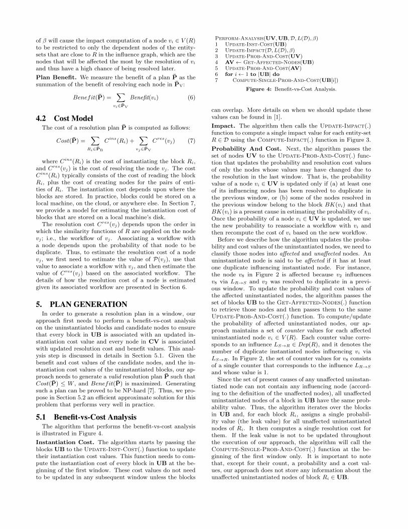
approach first needs to perform a benefit-vs-cost analysison the uninstantiated blocks and candidate nodes to ensurethat every block in UB is associated with an updated in-stantiation cost value and every node in CV is associatedwith updated resolution cost and benefit values. This anal-ysis step is discussed in details in Section 5.1. Given thebenefit and cost values of the candidate nodes, and the in-stantiation cost values of the uninstantiated blocks, our ap-proach needs to generate a valid resolution plan P̄ such thatCost(P̄) ≤ W , and Benefit(P̄) is maximized. Generatingsuch a plan can be proved to be NP-hard [7]. Thus, we pro-pose in Section 5.2 an efficient approximate solution for thisproblem that performs very well in practice.

5.1 Benefit-vs-Cost AnalysisThe algorithm that performs the benefit-vs-cost analysis

is illustrated in Figure 4.

Instantiation Cost. The algorithm starts by passing theblocks UB to the Update-Inst-Cost(.) function to updatetheir instantiation cost values. This function needs to com-pute the instantiation cost of every block in UB at the be-ginning of the first window. These cost values do not needto be updated in any subsequent window unless the blocks

Perform-Analysis(UV,UB,D, L(D), β)1 Update-Inst-Cost(UB)2 Update-Impact(D, L(D), β)3 Update-Prob-And-Cost(UV)4 AV← Get-Affected-Nodes(UB)5 Update-Prob-And-Cost(AV)6 for i← 1 to |UB| do7 Compute-Single-Prob-And-Cost(UB[i])

Figure 4: Benefit-vs-Cost Analysis.

can overlap. More details on when we should update thesevalues can be found in [1].

Impact. The algorithm then calls the Update-Impact(.)function to compute a single impact value for each entity-setR ∈ D using the Compute-Impact(.) function in Figure 3.

Probability And Cost. Next, the algorithm passes theset of nodes UV to the Update-Prob-And-Cost(.) func-tion that updates the probability and resolution cost valuesof only the nodes whose values may have changed due tothe resolution in the last window. That is, the probabilityvalue of a node vi ∈ UV is updated only if (a) at least oneof its influencing nodes has been resolved to duplicate inthe previous window, or (b) some of the nodes resolved inthe previous window belong to the block BK(vi) and thatBK(vi) is a present cause in estimating the probability of vi.Once the probability of a node vi ∈ UV is updated, we usethe new probability to reassociate a workflow with vi andthen recompute the cost of vi based on the new workflow.

Before we describe how the algorithm updates the proba-bility and cost values of the uninstantiated nodes, we need toclassify those nodes into affected and unaffected nodes. Anuninstantiated node is said to be affected if it has at leastone duplicate influencing instantiated node. For instance,the node v8 in Figure 2 is affected because v2 influencesv8 via LR→S and v2 was resolved to duplicate in a previ-ous window. To update the probability and cost values ofthe affected uninstantiated nodes, the algorithm passes theset of blocks UB to the Get-Affected-Nodes(.) functionto retrieve those nodes and then passes them to the sameUpdate-Prob-And-Cost(.) function. To compute/updatethe probability of affected uninstantiated nodes, our ap-proach maintains a set of counter values for each affecteduninstantiated node vi ∈ V (R). Each counter value corre-sponds to an influence LS→R ∈ Dep(R), and it denotes thenumber of duplicate instantiated nodes influencing vi viaLS→R. In Figure 2, the set of counter values for v8 consistsof a single counter that corresponds to the influence LR→S

and whose value is 1.Since the set of present causes of any unaffected uninstan-

tiated node can not contain any influencing node (accord-ing to the definition of the unaffected nodes), all unaffecteduninstantiated nodes of a block in UB have the same prob-ability value. Thus, the algorithm iterates over the blocksin UB and, for each block Ri, assigns a single probabil-ity value (the leak value) for all unaffected uninstantiatednodes of Ri. It then computes a single resolution cost forthem. If the leak value is not to be updated throughoutthe execution of our approach, the algorithm will call theCompute-Single-Prob-And-Cost(.) function at the be-ginning of the first window only. It is important to notethat, except for their count, a probability and a cost val-ues, our approach does not store any information about theunaffected uninstantiated nodes of block Ri ∈ UB.

Generate-Plan(UV,UB,W,D)1 BlockSet P̄B ← ∅2 NodeSet P̄V ← ∅, M ← ∅3 Double max, t4 〈P̄V,max〉 ← Select-Nodes(UV,W,D)5 BlockList List← Sort-Blocks(UB,D)6 for i← 1 to |List| do7 Block B ← List[i]8 〈M, t〉 ← Select-Nodes(P̄V ∪ V (B), W − Cins(B),D)9 if t > max then

10 P̄B ← P̄B ∪ {B}11 P̄V ←M12 max← t13 W ←W − Cins(B)14 else15 break16 return 〈P̄B, P̄V〉

Figure 5: Generating A Valid Resolution Plan.

5.2 AlgorithmOur algorithm that generates a valid resolution plan is

illustrated in Figure 5. The algorithm initially calls theSelect-Nodes(.) function (Line 4) to compute the maxi-mum benefit that can be obtained by considering only theinstantiated unresolved nodes UV. The input to this func-tion is a set of nodes, a cost budget, and the dataset D (theimpact values are associated with the entity-sets of D). Thisfunction first identifies a subset of the input nodes whose to-tal resolution cost is less than or equal to the input budgetand their total benefit is as large as possible, and then re-turns this subset of nodes along with their total benefit. Theimplementation of this function is discussed later. Then, thealgorithm sorts the blocks in UB in a non-increasing orderbased on their benefit that they are expected to add to thecurrent window once they are instantiated (Line 5). To sortthese blocks, the Sort-Blocks(.) function first computes,for each block Ri ∈ UB, a usefulness value as follows:

U(Ri) =

∑vj∈V (Ri)

Benefit(vj)

Cins(Ri) +∑

vj∈V (Ri)

Cres(vj)(8)

Then, the function sorts the blocks in a non-increasingorder based on their usefulness values and returns the sortedlist of blocks.

Next, the algorithm iterates over the sorted list of blocks,and for each block, checks if the total benefit that can beobtained in the window will increase if that block is instan-tiated (Lines 8-9). If so, the algorithm adds the block to theset of selected blocks P̄B, and updates the values of the setP̄V and the other helper variables (Lines 10-13). Otherwise,it exists the while loop. Finally, the algorithm returns thesets P̄B and P̄V (Line 16).

Select Nodes. The Select-Nodes(.) function chooses asubset of nodes from the input set such that their total ben-efit is maximized and their total cost is less than or equal tothe input budget. In general, the benefit of some nodes inthe input set might be dependent upon whether some othernodes in the input set have been added to the output set ofnodes or not. For example, consider the graph in Figure 2.For simplicity, suppose that the input set to this functionconsists of all candidate nodes. Let us further assume thatthe impact of each candidate node is computed using Equa-

tion 4 and that the node v8 ∈ N (v3). This means that thenode v8 was used in computing the current impact value ofv3, and thus the impact of v3 needs to be updated once v8is added to the output set of nodes.

Accounting for such dependency among the input nodesis infeasible in practice. To illustrate, suppose that theSelect-Nodes(.) function in the example above added v12to the output set. Since v12 belongs to an uninstantiatedblock and none of its influencing nodes is instantiated, de-termining which nodes to update as a result of this additionmight not be applicable unless the sets of influencing nodesof all nodes in G are known. Even if such information isavailable, accounting for the dependency among the nodesmight be unnecessary since the set of output nodes usuallyconstitutes a small percentage of the nodes in V , and hencethe likelihood that they will be dependent upon each otheris in general low. Such a likelihood will even decrease as thevalue of β decreases until it becomes zero at the later stagesof the execution when the benefit of nodes are restricted totheir direct benefit, i.e., their probability values.

Therefore, we do not account for such dependency amongthe nodes when determining the output set of nodes of theSelect-Nodes(.) function, viewing the problem as a tra-ditional knapsack problem. Hence, we use the greedy al-gorithm that first sorts the nodes in the input set in a de-creasing order based on their benefit per cost unit, and then,starting from the head of the sorted list, it proceeds to insertthe nodes into the output set until the budget is consumed.This greedy algorithm works very well in the cases where theitems’ weights (i.e., nodes’ resolution costs) are very smallrelative to the knapsack size.

Initialization Step. In the initial few resolution windows,our approach might not have adequate knowledge aboutwhich nodes tend to be duplicate and which blocks containa high number of duplicate nodes. To obtain such knowl-edge may require that our approach explores several blocksin the initial few windows. To address this requirement,the approach needs to employ a different strategy for gen-erating a resolution plan. Using the algorithm in Figure 5in such cases might result in instantiating a lesser numberof blocks than desired, and thus unnecessarily resolving alarge number of nodes of these blocks. To illustrate, sup-pose that the first two blocks in the sorted list returnedfrom the Sort-Blocks(.) function at the beginning of thefirst window belong to the same entity-set, i.e., all nodes ofthese two blocks have the same benefit per cost value. Inthis case, the algorithm in Figure 5 will not consider instan-tiating the second block unless the budget W is sufficient forinstantiating and resolving all nodes of the first block. How-ever, our approach may want to instantiate several blocksin each of the initial few windows and explore those blocksby resolving a few nodes from each of them.

The plan generation algorithm that we use in each of theseinitial windows is a modification of the algorithm shown inFigure 5. It first starts by sorting the blocks in UB us-ing the same Sort-Blocks(.) function. Then, it iteratesover the blocks in the sorted list, starting from the headof the list. For each block Ri, the algorithm checks if theinstantiation cost of this block plus the cost of resolvingk randomly chosen nodes of Ri, denoted as Cr(Ri, k), isless than or equal to the remaining budget of the currentwindow, where k = dα ∗ |V (Ri)|e and the value α is thethreshold described in Section 4.1. If so, the algorithm in-

serts Ri and the k nodes into the sets P̄B and P̄V respec-tively, and then updates the window budget accordingly;i.e., W = W −Ci(Ri)−Cr(Ri, k). Otherwise, the algorithmconsiders the next block in the sorted list and performs thesame steps on it. This process continues until the budget Wis consumed or we have iterated over all blocks in the sortedlist. Finally, if W is not fully consumed, the algorithm ran-domly chooses extra nodes from the blocks in P̄B and addsthem to the set P̄V to fill the budget W . This algorithmcan be viewed as an initialization step of our approach andtherefore be employed in the initial few windows.

6. WORKFLOWSGiven |FR| similarity functions associated with entity-set

R, there are |FR|! different orders of function applicationthat could be employed to resolve a node vi ∈ V (R). We,however, should apply these functions in the order that leadsto a certain resolution decision with the least amount of cost.To generate such an order, we need to differentiate betweenthese functions in terms of their costs and their contribu-tions to the resolution decision of a node. In this section,we first define our concept of the contribution of similarityfunctions, then describe how workflows are generated andassociated with nodes, and finally show how we can estimatethe resolution cost of a node given its associated workflow.

Function Contribution. In order to resolve a node vi, weneed to obtain sufficient positive or negative evidence. Eachsimilarity function fR

j , when applied on a node vi, providespositive and/or negative evidence to the resolution of vi.Evidence is considered positive (negative) if it will increasethe chance that the resolve function will return 1 as thesimilarity (dissimilarity) confidence of vi. The amounts ofthe positive and negative evidence of fR

j are measured bythe resolve function <R when it is applied later on vi.

Similarity functions differ from each other in terms of theamount of evidence that they provide to the resolution deci-sion. Therefore, in order to generate a workflow for a nodevi ∈ V (R), we need to estimate the amount of positive andnegative evidence that the similarity functions in FR pro-vide w.r.t. the function <R. Hence, we define for eachfunction fR

j , a positive contribution tR+j ∈ [0, 1], and a neg-

ative contribution tR−j ∈ [0, 1]. The positive contribution ofa function is the amount of positive evidence that the func-tion is expected to provide when it is applied on a duplicatenode. Similarly, the negative contribution of a function isthe amount of negative evidence that the function is ex-pected to provide when it is applied on a distinct node.

Workflow Generation. The process of generating a work-flow for a node vi ∈ V (R) proceeds as follows. First, wecompute for each similarity function fR

j ∈ FR a utility value

as follows: [θ∗tR+j +(1−θ)∗tR−j ]/cRj , where θ is set to P(vi).

Then, we sort the functions in FR in a non-increasing orderbased on their utility values. This order of functions is theworkflow of vi. This sorting will place the functions withthe highest contribution per unit cost of resolution first inthe workflow, maximizing the chance of resolving vi to acertain decision with the least amount of cost.

Workflow Association Strategy. As explained in Sec-tion 5, to estimate the resolution cost of a node requiresknowing the workflow that will be used to resolve that node.One naive strategy of associating a workflow with a node viis to instantly generate a workflow for vi as discussed above.

Such a strategy can be inefficient as we will have to sort thesimilarity functions every time we need to estimate the reso-lution cost of a node. Thus, we follow a more efficient strat-egy for associating a workflow with a node. This strategyrequires that we maintain a set of w pre-generated workflowsWR

1 ,WR2 , . . . ,W

Rw for each entity-set R ∈ D. Each workflow

WRk is generated as described above with the value of θ set

to k−1w−1

. For example, if w = 5, then the θ values that we useto generate these w workflows will be: 0, 0.25, 0.5, 0.75, and1.0 respectively. Now, to associate a workflow with a nodevi ∈ V (R), we can simply map the node vi to the workflowWR

k whose θ value, i.e., k−1w−1

, is the closet (among all the

workflows’ of R) to the value of P(vi).

Resolution Cost. Given a node vi ∈ V (R) and its work-flow WR

k , we estimate the value of Cres(vi) as follows:

Cres(vi) = P(vi) ∗Cr+(WRk ) + (1−P(vi)) ∗Cr−(WR

k ) (9)

where Cr+(WRk ) is the expected cost that should be in-

curred to resolve a duplicate node using the workflow WRk ,

and Cr−(WRk ) is the expected cost that should be incurred

to resolve a distinct node using the workflow WRk . Such

values can be easily learned from a training dataset.

7. EXPERIMENTAL EVALUATIONIn this section, we evaluate the quality and efficiency of

our approach on publication and synthetic datasets.

7.1 Experimental SetupBlock Instantiation Cost. In our experiments, the pub-lication and synthetic datasets are initially stored on disk.Each block Ri is stored in a single file that contains the en-tities of Ri along with their dependency information, i.e.,which entities are dependent upon the entities of Ri via in-fluence LR→S ∈ Inf(R)5. However, the information of whichblocks those dependent entities belong to is stored in differ-ent files. Thus, the instantiation/loading cost of block Ri

can be estimated as follows:

Cins(Ri) = Cf (Ri) + |V (Ri)| ∗ cc+∑

LR→S∈Inf(R)

Cb(S) (10)

where Cf (Ri) is the cost of reading the file that containsthe block Ri from disk and it is a function of the numberand the size of entities in Ri, cc is the cost of constructing anode for a pair of entities, and Cb(S) is the cost of readingthe blocking information of the referenced entities of S.

Algorithms. In our experiments, we compare our solutionwith the DepGraph algorithm proposed in [12]. Althoughthis algorithm is not a progressive solution, it is one ofthe few algorithms that resolve entities of multiple differenttypes simultaneously without having to divide the resolu-tion based on the entity type. In addition, we compare oursolution with three variants of our approach. The first one,referred to as Static, differs from our approach only in howthe Sort-Blocks(.) function in Figure 5 sorts the blocks.In this variant, the order of the blocks is statically deter-mined at the beginning of the execution as follows. First,we sort the entity-sets based on their influences accordingto [23]. For example, if Inf(R) = {LR→T }, Inf(S) = ∅, and

5Each entity-set R has as many reference attributes as the number

of influences in Inf(R). The value of a reference attribute (that cor-responds to an influence LR→S) for entity ri contains the IDs of theentities of S that are dependent upon ri via LR→S (as in Table 1).

0.1

0.2

0.3

0.4

0.5

0.6

0.7

0.8

0.9

1

40 80 120 160 200 240 280 320 360 400 440 480 520 560

Dup

licat

e R

ecal

l

Execution Time (Sec)

Our ApproachStatic

DepGraph

Figure 6: Time vs. Recall.

0.1

0.2

0.3

0.4

0.5

0.6

0.7

0.8

0.9

1

5 10 15 20 25 30 35 40 45 50 55 60 65

Dup

licat

e R

ecal

l

Execution Time (Sec)

Our ApproachStatic

DepGraph

(a) z = 0.

0.1

0.2

0.3

0.4

0.5

0.6

0.7

0.8

0.9

1

5 10 15 20 25 30 35 40 45 50 55 60 65

Dup

licat

e R

ecal

l

Execution Time (Sec)

Our ApproachStatic

DepGraph

(b) z = 0.15.

0.1

0.2

0.3

0.4

0.5

0.6

0.7

0.8

0.9

1

5 10 15 20 25 30 35 40 45 50 55 60 65

Dup

licat

e R

ecal

l

Execution Time (Sec)

Our ApproachStatic

DepGraph

(c) z = 0.3.Figure 7: Effects of Zipfian Distribution Exponent Value.

Inf(T ) = {LT→S}, then R’s blocks will appear first in thesorted list of blocks, then T ’s blocks, and finally S’s blocks.Then, blocks of the same entity-set are sorted in a randomfashion. The second variant, referred to as All, does not usethe lazy resolution strategy. That is, when resolving a nodevi ∈ V (R), it applies all the similarity functions of R on thatnode and then calls the resolve function to determine its res-olution decision. The third variant, referred to as Random,uses the lazy resolution strategy but applies the similarityfunctions on a node in a random order.

Quality Metric. Since the goal of our approach is to findand resolve as many duplicate pairs as possible using thebudget BG, we use the duplicate pairwise recall as our qual-ity metric. Duplicate recall is the ratio of the correctly re-solved duplicate pairs to the total number of duplicate pairsin the ground truth. We do not use the duplicate preci-sion (the ratio of the correctly resolved duplicate pairs tothe total number of resolved duplicate pairs) because ourapproach always achieves more than 0.99 precision.

7.2 Publication Dataset ExperimentsIn this section, we evaluate the efficacy of our approach

on a real publication dataset called CiteSeerX [2]. We ob-tained a subset of 30, 000 publications from the entire col-lection, and then extracted from those publications infor-mation regarding Papers (P ), Authors (A), and Venues (U)according to the following schema: Papers (Title, Abstract,Keywords, Authors, Venue), Authors (Name, Email, Affil-iation, Address, Papers), and Venue (Name, Year, Pages,Papers). The cardinalities of the resultant entity-sets are|P | = 30, 000, |A| = 83, 152 and |U | = 30, 000. We com-puted the ground truth by simply running the DepGraphalgorithm on the obtained dataset.

Each entity-set is divided into a set of blocks. We usetwo blocking functions to partition entity-set P into a set ofoverlapping blocks. The first function partitions the entitiesbased on the first three characters of their titles, whereas thesecond function partitions them based on the last three char-acters of their titles. Also, we use a blocking function thatpartitions entity-set A into blocks based on the first char-acter of the author’s first name appended with the first twocharacters of his/her last name. Similarly, we use a block-ing function that partitions entity-set U into blocks basedon the first two characters of the venue name appended withthe first two digits of the venue year.

For this dataset, we use the same set of similarity func-tions given in Table 2 with the addition of four functionsfA3 , fA

4 , fU2 , and fU

3 . These four functions are defined onthe A.Affiliation, A.Address, U .Year, and U .Pages respec-tively, and use the edit distance algorithm to compute thesimilarity between their input values. The resolve function

of each entity-set is implemented as a Naive Bayes classifier.

Experiment 1 (Cost-vs-Recall). Figure 6 plots the du-plicate recall as a function of the resolution cost (measuredas the end-to-end execution time) for various ER algorithms.In the Static approach, P ’s blocks appear first in the sortedlist of blocks, then A’s blocks, and finally U ’s blocks. Inthis experiment, we do not study the benefit of using thelazy resolution strategy in resolving nodes. Therefore, whenresolving a pair of entities, all algorithms in Figure 6 applyall the corresponding similarity functions on that pair evenif some of them are sufficient to resolve the pair.

To plot the curve of our approach, we ran the approachwith different budget values (correspond to the points onthe curve). For each budget value, we ran the approach tentimes, recorded the achieved recall of each run, and then re-ported the average recall of the ten recall values. The curveof the Static approach is plotted in the same way as we plot-ted the curve of our approach. For the DepGraph approach,we ran it to completion ten times, recorded the completiontime of each run, and then took the average completion timeof the ten values. Then, the recall corresponding to any bud-get value is set to zero if that budget value is less than theaverage completion time, or to one otherwise.

The results in Figure 6 show how our approach can achievehigh duplicate recall values using limited budget values. Theperformance gap between our approach and the Static ap-proach demonstrates the importance of employing a goodstrategy for selecting which blocks to load into memorynext. The DepGraph approach is not progressive, and thusit reaches the maximum recall only after resolving the en-tire dataset. Note that the two progressive approach needmore time, compared to the DepGraph algorithm, to reachthe maximum recall. This amount of extra time representsthe overhead that these approaches need to incur to performprogressive resolution.

Experiment 2 (Lazy Resolution and Execution TimePhases). This experiment studies the benefit of resolvingthe nodes using the lazy resolution strategy with workflows.

Our Approach Random All

Execution Time (sec) 300.33 396.55 542.43Plan Generation 4.76% 3.81% 2.58%Graph Creation 8.40% 6.25% 4.72%Reading Blocks 4.70% 3.75% 2.90%Node Resolution 82.01% 86.17% 89.78%

Table 3: Phases of Execution Time.

To conduct this experiment, we ran each of the three ap-proaches shown in Table 3 ten times with the minimum bud-get value (the end-to-end execution time) that is sufficientfor the approach to resolve all pairs in the dataset (i.e., ap-ply the similarity functions on every pair). For each run,

we recorded the exact total execution time (the first row inTable 3) along with the breakdown of that execution time(the times spent on generating plans, on reading blocks, oncreating the graph, and on resolving nodes). Next, we tookthe average of those values, and reported them in Table 3.For example, we ran our approach with BG = 310 secondsten times, and found that on average our approach finishesin 300.33 seconds and that the plan generation process (Sec-tion 5) takes on average 4.76% of the total exact executiontime, whereas the plan execution process takes on average95.11% (4.7% for reading blocks from disk, 8.4% for incre-mentally creating the graph, and 82.01% for resolving thenodes). The achieved recall of each approach using the spec-ified time is 1.0.

This experiment demonstrates the following. First, usingthe lazy resolution strategy with workflows can significantlyreduce the cost of applying the similarity functions on thenodes. This, in turn, offers the flexibility for developers toplug in multiple similarity functions of various cost and con-tribution values without having to worry about the cost ofapplying those functions as our approach can systematicallyresolve the nodes with the least amount of cost. Second, thepercentage of the plan generation process decreases as thecost of resolving the nodes increases. In general, modernER solutions employ more computationally expensive simi-larity functions, e.g., [19, 21], and therefore the overhead ofgenerating resolution plans in such cases can be even lower.

Parameter n s b d z l k

Value 4 20, 000 100 0.2 0.15 0.3 2

Table 4: Parameters of Synthetic Datasets.

7.3 Synthetic Dataset ExperimentsIn order to evaluate our approach in a wider range of

various scenarios, we built a synthetic dataset generator thatallows us to generate datasets with different characteristics.The parameters that this generator takes as input along withtheir default values are shown in Table 4.

In each synthetic dataset, we generate n entity-sets, eachcontains s entities. The s entities of each entity-set are di-vided evenly into b non-overlapping blocks. The parameterd is the fraction of duplicate pairs in each entity-set, and itis computed as the number of duplicate pairs divided by thetotal number of pairs after applying blocking. The dupli-cate pairs of an entity-set are distributed across the blocksof that entity-set using a zipfian distribution with an expo-nent of z. The parameter l ∈ [0, 1] determines the number ofinfluences in the dataset. For each two entity-sets R and S,there is an influence from entity-set R to entity-set S withprobability l. Thus, the higher the value of l is, the higherthe number of influences in the dataset will be. Finally, theparameter k represents the average number of direct depen-dent nodes that each node vi ∈ V (R) can have via eachinfluence LR→S ∈ Inf(R). We require the direct dependentnodes of a duplicate node to be also duplicate, and the directdependent nodes of a distinct node to be also distinct.

Each entity-set R has one non-reference twenty-five char-acter long string attribute, and is associated with a singlesimilarity function that is defined on that attribute. Thisfunction uses the edit-distance algorithm to compute thesimilarity between the values of that attribute. The resolvefunction of each entity-set employs a simple decision-making

0.1

0.2

0.3

0.4

0.5

0.6

0.7

0.8

0.9

1

5 10 15 20 25 30 35 40 45 50 55 60 65 70 75

Dup

licat

e R

ecal

l

Execution Time (Sec)

Our ApproachStatic

DepGraph

(a) l = 0.

0.1

0.2

0.3

0.4

0.5

0.6

0.7

0.8

0.9

1

5 10 15 20 25 30 35 40 45 50 55 60 65 70 75

Dup

licat

e R

ecal

l

Execution Time (Sec)

Our ApproachStatic

DepGraph

(b) l = 0.6.Figure 8: Effects of the Number of Influences.

process; it returns 1 as the similarity (dissimilarity) confi-dence of a pair only if the associated similarity function hasbeen applied on the pair and indicated that the two valuesof the string attribute are similar (distinct).

Experiment 3 (Effects of Duplicate Distribution). Inthis experiment, we study the performance of various ERalgorithms when varying the value of the exponent z whilefixing the other parameters to their default values. Whenz = 0, all blocks have the same effect on the duplicate recallbecause the duplicate pairs are uniformly distributed acrossall blocks of the dataset. However, in the cases where theduplicate pairs are not uniformly distributed, resolving theblocks with high duplicate percentage will have higher in-fluence on the duplicate recall than resolving those with lowduplicate percentage. Therefore, the higher the value of zis, the smaller the number of blocks that have the highestinfluence on the duplicate recall. In Figure 7, we vary thevalue of z from 0 to 0.3. Each figure in Figure 7 was plottedin the same way as we plotted Figure 6. As shown in thesefigures, the higher the value of z is, the better our approachperforms compared to the other algorithms.

This experiment demonstrates the following. First, ourapproach performs well even when the resolution cost is rel-atively cheap (involves applying a single similarity functionon two twenty-five character long string values). Second, ourapproach can adapt itself to datasets with various duplicatedistributions and therefore quickly identify and resolve theblocks with high duplicate percentage values. Third, ourapproach is more effective when the duplicate pairs are notuniformly distributed across the blocks which is almost al-ways the case in real-world datsets.

Experiment 4 (Effects of Influences). In this experi-ment, we study the effects of the number of influences onthe performance of various ER approaches. In Figure 8, wevary the value of l from 0 to 0.6. The result when l = 0.3 isplotted in Figure 7(b). Each figure in Figure 8 was plottedin the same way as we plotted Figure 6.

As expected, when l = 0, our approach behaves very sim-ilarly to the Static approach because there exists no influ-ences that our approach can utilize to identify which blocksto load and which nodes to resolve next. In fact, the Staticapproach performs slightly better than our approach be-cause it does not need to compute the usefulness valuesof the blocks and then sort them in each window. How-ever, as the value of l increases, our approach starts to per-form better than the Static approach because the number ofinfluences increases and that therefore implies that declar-ing a node to be duplicate can guide us towards findingsmore duplicate nodes in the dataset. On the other hand,the increase in the number of influences introduces a littleoverhead in performing the benefit-vs-cost analysis in the

two progressive approaches (as more influences are involvedwhen computing the probability and impact values), andin loading the blocks into memory in the three approaches.This, therefore, causes the approaches to run a little slower.

This experiment also emphasizes the importance of em-ploying a proper block selection strategy because even whenl is 0.6, the Static approach can achieve only around 0.77%recall with the same amount of time that the DepGraph al-gorithm needs to resolve the entire dataset.

8. RELATED WORKEntity resolution is a well-known data quality problem

and has received significant attention in the literature overthe past few decades, e.g., [5, 8, 23, 24]. Most prior work inthis area has focused on improving either the efficiency of theER algorithms [14,18] or the quality of their results [4,6,24].However, only a few research efforts have considered theproblem of exploring a trade-off between the quality of theresult and the resolution cost [9, 15,22].

The most related work to our paper is that of [22]. Asstated in Section 1, the context/type of datasets for whichthe two approaches have been developed differs. In fact,this difference raises an interesting question. To resolve arelational dataset D using a limited budget, should we useour approach, or should we resolve each entity-set in isola-tion using a single entity-set ER algorithm (that does notexploit the relationships in D) with the help of one of thehints proposed in [22]? Our approach is intended for situ-ations where exploiting those relationships is important inresolving D. If those relationships are not important (i.e.,the similarity between the attribute values is sufficient toachieve high-quality results), then using our approach maynot provide any significant advantage over [22]. A full char-acterization of under what circumstances one should choosewhich approach is an interesting direction of future work.

Furthermore, the problem of relational entity resolutionhas been studied in the literature. Reference [11] proposesa probabilistic model that uses Conditional Random Fields(CRF) to capture the dependencies between different entity-sets. In [12], the algorithm performs the resolution processon different entity-sets simultaneously. The relationshipsamong entity-sets are leveraged to propagate the similarityincreases of some pair to its dependent pairs. Moreover, theauthors in [23] propose a joint ER framework for resolvingmultiple datasets in a parallel fashion using custom ER al-gorithms. This proposed framework is not designed to bea progressive solution; thus the order in which the datasetsare resolved is determined at the beginning of the joint ERalgorithm. Our solution, however, dynamically specifies theorder in which the blocks are resolved based on the estimatedamount of data quality issues in these blocks.

9. CONCLUSIONSIn this paper, we have proposed a progressive approach

to relational ER wherein the input dataset is resolved usingonly a limited budget with the aim of maximizing the qualityof the result. Our approach follows an adaptive strategy thatperiodically monitors the resolution progress to determinewhich parts of the dataset should be resolved next and howthey should be resolved. We showed empirically how ourapproach can quickly identify and resolve the duplicate pairsin the dataset, and thus generate a high quality result usinglimited amounts of resolution budget.

10. ACKNOWLEDGMENTSThis work was supported in part by NSF grants III-1429922,

III-1118114, CNS-1059436, and by DHS grant 206-000070.Yasser Altowim was supported by KACST’s Graduate Stud-ies Scholarship.

11. REFERENCES[1] http://ics.uci.edu/~yaltowim/ProgER.pdf.

[2] http://csxstatic.ist.psu.edu/about/data.[3] H. Altwaijry, D. V. Kalashnikov, and S. Mehrotra.

Query-driven approach to entity resolution. In VLDB, pp.1846–1857, 2013.

[4] R. Ananthakrishna, S. Chaudhuri, and V. Ganti.Eliminating fuzzy duplicates in data warehouses. In VLDB,pp. 586–597, 2002.

[5] O. Benjelloun, H. Garcia-Molina, D. Menestrina, Q. Su,S. E. Whang, and J. Widom. Swoosh: a generic approachto entity resolution. VLDB J., pp. 255–276, 2009.

[6] I. Bhattacharya and L. Getoor. Collective entity resolutionin relational data. TKDD, pp. 1–36, 2007.

[7] J. J. Burg, J. Ainsworth, B. Casto, and S.-D. Lang.Experiments with the oregon trail knapsack problem.Electronic Notes in Discrete Mathematics, 1:26–35, 1999.

[8] Z. Chen, D. V. Kalashnikov, and S. Mehrotra. Exploitingcontext analysis for combining multiple entity resolutionsystems. In SIGMOD, pp. 207–218, 2009.

[9] R. Cheng, E. Lo, X. S. Yang, M.-H. Luk, X. Li, and X. Xie.Explore or exploit?: effective strategies for disambiguatinglarge databases. In VLDB, pp. 815–825, 2010.

[10] G. F. Cooper. The computational complexity ofprobabilistic inference using bayesian belief networks.Artificial intelligence, 42(2):393–405, 1990.

[11] A. Culotta and A. McCallum. Joint deduplication ofmultiple record types in relational data. In CIKM, pp.257–258, 2005.

[12] X. Dong, A. Halevy, and J. Madhavan. Referencereconciliation in complex information spaces. In SIGMOD,pp. 85–96, 2005.

[13] M. Henrion. Practical issues in constructing a bayes’ beliefnetwork. In UAI, pp. 132–139, 1987.

[14] M. Hernandez and S. Stolfo. The merge/purge problem forlarge databases. In SIGMOD, pp. 127–138, 1995.

[15] S. R. Jeffery, M. J. Franklin, and A. Y. Halevy.Pay-as-you-go user feedback for dataspace systems. InSIGMOD, pp. 847–860, 2008.

[16] F. V. Jensen and T. D. Nielsen. Bayesian networks anddecision graphs. Springer, 2007.

[17] J. F. Lemmer and D. E. Gossink. Recursive noisy or - arule for estimating complex probabilistic interactions.Trans. Sys. Man Cyber. Part B, pp. 2252–2261, 2004.

[18] A. K. McCallum, K. Nigam, and L. Ungar. Efficientclustering of high-dimensional data sets with application toreference matching. In SIGKDD, pp. 169–178, 2000.

[19] R. Nuray-Turan, D. V. Kalashnikov, and S. Mehrotra.Exploiting web querying for web people search. In TODS,pp. 7:1–7:41, 2012.

[20] J. Pearl. Probabilistic reasoning in intelligent systems:networks of plausible inference. Morgan Kaufmann, 1988.

[21] J. Wang, T. Kraska, M. J. Franklin, and J. Feng. Crowder:Crowdsourcing entity resolution. In VLDB, pp. 1483–1494,2012.

[22] S. Whang, D. Marmaros, and H. Garcia-Molina.Pay-as-you-go entity resolution. In TKDE, pp. 1111–1124,2013.

[23] S. E. Whang and H. Garcia-Molina. Joint entity resolution.In ICDE, pp. 294–305, 2012.

[24] M. Yakout, A. K. Elmagarmid, H. Elmelegy, M. Ouzzani,and A. Qi. Behavior based record linkage. In VLDB, pp.439–448, 2010.