bec for interacting bosons - iam.uni-bonn.de

BEC for interacting bosons

Serena Cenatiempo

joint work with A. Giuliani

L’Aquila, 22 March 2012

A separation is effected; one part condenses,the rest remains a saturated ideal gas.Einstein, 1925

MotivationsKnown results

The model and sketch of the proofPerspectives

Motivations

Since 1995 BEC of dilute atomic gases has been subject ofintensive studies, driven by new experimental techniques:

I quantum systems unique in the precision and flexibility,wherewith they can be manipulated;

I ultralow-temperature laboratories for atom optics,collisional physics, many-body physics, superfluidity,quantized vortices;

I great variety of applications: atom laser, qubitsand quantum fluids.

Hansel et al. (2001)

Nature Physics 1 (2005)Billy, Josse, Zuo, Guerin, Aspect, Bouyer (2008)

S. Cenatiempo BEC for interacting bosons



Motivations

Experiments on gases in flat or elongatedtraps also motivate the study of BECin low dimensional systems.

Clade et al. (2009)

Kruger et al. (2007)

State of the art:

From a theoretical point of view, there are very few (quite special) modelsin which we are able to prove Bose condensation for interacting bosons.




Sketch of the result

We have studied the problem of Bose condensation at zero temperature andweak coupling for a system of bosons in d = 2, 3 interacting with a repulsiveshort range potential, in the presence of an ultraviolet cutoff, proving that:

I the interacting theory is well defined at all orders interms of an effective parameter related to theintensity of the interaction;

I the correlations does not exhibit anomalousdimensions, i.e. the model is in the same universalityclass of the exactly soluble Bogoliubov model.

→ strong justification of the validity at all ordersof Bogoliubov theory also in d = 2




Bogoliubov approximationBogoliubov predictionBeyond Bogoliubov

Bogoliubov approximation (1947)

Basic Hamiltonian of the problem:

H =N∑

i=1

(−∆xi − µ) + λ∑i<j

v (xi − xj )

where

the scene of action is a periodic box in R3 of side size L

xi is the coordinate of the i th particle

N is the number of bosons

The pair potential λv (xi − xj ) is C∞ and short range

We are interested in the bulk limit: N →∞ with ρ = costant.






Hamiltonian in momentum space: a+k and ak are

boson creation/annihilation operators

H =∑k

k2a+k ak +

1

2V

∑k,q,p

a+k+pa

+q−pλv(p)akaq

v(p)

q

q− p

k

k+ p

At zero temperature, in the non interacting case:

Nk =⟨a+

k ak

⟩= Nδk,0

Condensation hypothesis:

At weak coupling N>0

N 0� 1






Hamiltonian in momentum space: a+k and ak are

boson creation/annihilation operators

H =∑k

k2a+k ak +

1

2V

∑k,q,p

a+k+pa

+q−pλv(p)akaq

v(p)

q

q− p

k

k+ p

By the substitution a+0 = a0 =

√N:

HB =1

2VN(N − 1)λv(0) +

∑k6=0

[k2 +

N

Vλv(k)

]a+k ak

+1

2Vλ∑k6=0

v(k)N[a+k a

+−k + aka−k

]+ (cubic and quartic terms)

Due to the condensation hypothesis the cubic and quartic terms may beexpected to be small in comparison with the quadratic ones.





Bogoliubov prediction

HB is a quadratic form in the a’s and may be diagonalized:

H ′B = E0(ρ) +∑k6=0

ε(k) b+k bk

I Spectrum:

ε(k) =√

k4 + 2λρv(k)k2 '|k|→0

√2λρv(0)|k| = vB |k|

→ Landau argument for superfluidity

I Ground state energy at low density and in the thermodynamic limit:

E0(ρ) =1

2Nλρv(0)− N

2ρ

∫ddk

(2π)d

{k2 + λρv(k)− ε(k)

}In the regime ρv(0)� R−1

0 we can approximate v(k) ' v(0) andcalculate the integral explicitly.





Bogoliubov ground state d = 3

In the regime ρa� R−10 , with a the scattering length of the two body

potential, Bogoliubov prediction is

E0(ρ) 'ρa3→0

4πNρa

(1 +

128

15√π

√ρa3 + . . .

)Remarks:

I The first term is the number of pairs of particles N(N − 1)/2 times theg.s. energy of two particles in a large box Λ, 8πa/|Λ|

I The contribution coming from the neglected cubic and quartic terms is oforder ρa3 log (ρa3)

I The leading term was proved by Dyson (upper bound, 1957) andLieb-Yngvason (lower bound, 1998); the second order correctionwas first computed by Lee-Huang-Yang (1957) but its proof is, so far,an open problem.





Bogoliubov ground state d = 2

Condensation is expected only for zero temperature(Mermin-Wagner-Hohenberg theorem)

Ground state energy per particle of a dilute, homogeneous, 2d Bose gasin the thermodynamic limit 1: e0(ρ) ' 4πρ| log ρa2|−1

Remarks:

I In d = 2 the number of pairs of particles times the ground state energy oftwo particles in a large box would give 4πρ| log(a2/L2)|−1

I Bogoliubov prediction for R−10 �

√λρ is 2

e0(ρ) =λρ

2

(1 + O(log(λρR2

0 )))

=ρR2

0 =1

4πρ

| log ρa2|

(1 + O(log(| log ρa2|))

)with a the 2d scattering length, i.e. a = R0e

− 4πλ .

1 Schick (1971) and Lieb,Yngvason (2001)2 Hines et al., Hard disc Bose gas (1978)





Beyond Bogoliubov

Bogoliubov approximation assumes that, for sufficiently weak coupling, acondensed state still exists. This assumption is not a priori justified.

Bogoliubov scheme is valid for a Bose gas in arbitrary dimension in themean field limit (Seiringer 2010)

The calculation of the next corrections to Bogoliubov prediction for theg.s. energy is an open problem even if a few recent papers present partialresults.3

BEC has been proved in the special case of hard core bosons on a latticeat half-filling; estimates on a few correlation functions have beenestablished.

Lieb, Seiringer and Yngvason (2002) have proved Bose condensation andsuperfluidity for 3D and 2D bosons in a trap, but only in theGross-Pitaevskii limit, in which the density scales with the particle number.

3 Erdos, Schlein, Yau. Ground-state energy of a low-density Bose gas: a second-order upperbound. (2008); Giuliani, Seiringer.The ground state energy of the weakly interacting Bose gas athigh density. (2009)





Beyond Bogoliubov: perturbation theory

Numerous papers were then devoted to analyze the correctionsto Bogoliubov model: Beliaev (1958) , Gavoret and Nozieres(1964), Nepomnyashchy and Nepomnyashchy (1978), Popov(1987), Nozieres and Pines (1990). They all encountered thedifficulty of a singular perturbation theory plagued by infrareddivergence.





Beyond Bogoliubov: perturbation theory

Benfatto (1994)

First systematic study of the IR divergences for the 3d problem with anultraviolet momentum cutoff: the theory is order by order finite in therenormalized coupling constants, with the coefficients of order n bounded byn!|λ|n. → justification of the generally accepted picture of BEC√

scheme suitable for possible non perturbative treatments of the theory.

X requires the study of the flows of seven renormalized couplings.

X the 2d case is not approachable being the three and four bodyinteractions relevant in the renormalization group sense.





Pistolesi, Castellani, Di Castro, Strinati (1997, 2004)

Problem investigated for d = 2, 3 implementing local Ward identities in a RGapproach and exploiting a dimensional regularization with ε = 3− d . → ind = 2 non trivial fixed point and no anomalous dimensions.√

the WIs greatly simplify the study of the flow’s equations;√

the WIs are crucial in order to control the 2d theory;

X the dimensional regularization scheme does not allow to perform a fullnon perturbative construction even in principle.

Plan of the work

I To understand the local WI within the constructive RG scheme.

I The ultraviolet momentum cutoff explicitly breaks local gauge invariance.

↪→ In low-dimensional systems of interacting fermions (Luttinger liquidsa )the corrections to WI are crucial for establishing the infrared behavior ofthe system.

a Benfatto, Falco, Mastropietro (2009)




RG approachThe strategyWard IdentitiesResults

Functional integral representation

The partition function of thesystem can be formally expressedas a functional integral:

Z = e−E0|Λ| =∫

ΛP(dϕ) e−V (ϕ)

ϕ±x → creation and the annihilation operators for the bosons

ϕ±x = eHtϕ±x e−Ht , x = (t, x), Λ =

[−β

2, β

2

]×[− L

2, L

2

]d

V (ϕ) = λ2

∫dxdy |ϕx |2v(x− y)δ(x0 − y0)|ϕy |2 + ν0

∫dx |ϕx |2

P(dϕ) complex Gaussian measure ϕ+x = (ϕ−x )∗∫

ϕ−x ϕ+x P(dϕ) =

L,β→+∞ρ0 +

1

(2π)d+1

∫dd+1k

e−ikx

−ik0 + k2

Singular perturbation theory → ultraviolet and infrared divergences





The model

Since the condensation problem depends only on the long-distancebehaviour of the system we shall consider the following model:

g≤0(x) =1

(2π)d+1

∫ddkdk0 χ(|k | ≤ R−1

0 )e−ikx

−ik0 + k2

Due to the presence of the ultraviolet cutoff we can approximatev(k) = v(0)

For any finite β and L the theory is order by order finite, with β and Lplaying the role of an infrared cutoff.

The Renormalization Group approach consists in performing suitableresummations that make the resummed series finite at all orders uniformlyin the infrared cutoff and finally to send β and L to infinity.





The strategy

1 We fix the condensate density ρ0 and show that one can fix the chemicalpotential ν = ν(λ, ρ0) so that the interacting propagator g int(x) −→

x→∞ρ0

2 We write the bosonic fields as a sum of two independent gaussian fieldsϕ±x = ξ± + ψ±x with

⟨ξ−ξ+

⟩= ρ0. The ψ±x fields represent the fluctuations

with respect the condensate.

Z =∫P(dξ)e|Λ|W(ξ) W(ξ) = 1

|Λ| log∫e−V (ξ+ψ)P(dψ)

3 We perform perturbation theory around the gaussian measure thatcorresponds to Bogoliubov approximation:

PξB (dψ) =P(dψ) e−λv(0)∫

dx(ψ−x ξ

++ψ+x ξ

−)2

e|Λ|W(ξ) =

∫PξB (dψ) eV (ψ+ξ)





The strategy

y+

y-

( )V y

yl

yt

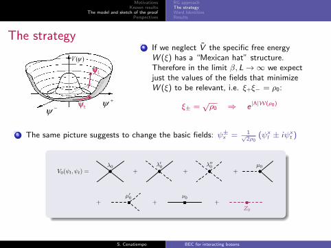
4 If we neglect V the specific free energyW (ξ) has a “Mexican hat” structure.Therefore in the limit β, L→∞ we expectjust the values of the fields that minimizeW (ξ) to be relevant, i.e. ξ+ξ− = ρ0:

ξ± =√ρ0 ⇒ e|Λ|W(ρ0)

5 The same picture suggests to change the basic fields: ψ±x = 1√2ρ0

(ψxl ± iψx

t )

V0(ψl, ψt) =λ0

+λ′0

+λ′′0

+µ0

+µ′0

+ν0

+Z0





Rigorous RG treatmentWe integrate iteratively the fields of decreasing scale of decreasing energyscale, i.e. such that k2

0 + λρ0k2 ' γ2hR−4

0 with γ > 1 and −∞ < h ≤ 0;the effective potential on scale h is

e−Vh(ψ) =

∫P

(h+1)B (dψ(h+1))e−Vh+1(ψ+ψ(h+1))

At each step we localize the relevant or marginal terms

LVh =λh

+µh

+γ2hνh

+Zh

+∂0 ∂0

Bh

+∂ ∂

Ah

+∂0

Eh

and include the quadraticterms in the freemeasure:

g−1≤h (k) = ρ

(k2Ah + k2

0R−20 Bh ik0Eh

−ik0Eh k2 + R20 Zh

)





Rigorous RG treatment

The result of this iterative integration is exactly written as a series in therunning coupling constants:

λh−1

=

λh

+ + +

µh−1

=µh

+ +

Zh−1

=Zh

+

Remark: Each step of this multiscale integration correspondsto a very large resummation of Feynman graphs.





Ward identities

By the gauge invariance of the generating functional W(ξ, φ) under thetransformation ψt,l

x → e iαψt,lx we obtain the following global WI

= =

λh = µh = Zh d = 3

γhλh = γh2 µh = Zh d = 2

and local (formal) WI

∂0

Eh

=J0

µJ0

h

∂0 ∂0

Bh

=∂0

J0

EJ0

h

∂ ∂

Ah

=∂

J1

EJ1

h

Eh

Zh−−−−→h→−∞

ε−1 ε = λρ0Rd0

Bh −−−−→h→−∞

ε−1

Ah −−−−→h→−∞

1 + o (1)

The flow of νh is controlled bythe choice of the chemical potential:

γ2hνh −→h→−∞

0





Correction to WI

The extra terms appearing in the Ward identities due to the presence of theultraviolet momentum cutoff give corrections of higher order in ε with respectto the formal WI.

∂0

Eh

=J0

µJ0

h

+

J0

∂0

∂0 ∂0

Bh

=∂0

J0

EJ0

h

+∂20

J0

∂ ∂

Ah

=∂

J1

EJ1

h

+∂2

J1

The strategy used does not require any hypothesis on the behaviour of λh

so the same arguments can be used in the 2d and 3d case.





Results

I Through the WIs the number of independent renormalized couplingconstants is reduced to one.

∗ for d = 2 an extra marginal couplingappears, λh

6, whose flow can be controlledusing one extra global WI.

λh6

I The theory is order by order finite in the renormalized couplingconstants provided that

d = 3 λh −−−−−→h→−∞

0

d = 2 λh −−−−−→h→−∞

λ∗ = const.

∗ for d = 3 one can prove that λh has an asintotically free flow in theinfrared limit;

∗ for d = 2 a second order calculation suggests λ∗ to be of order one.





Results: renormalization of the measure

The Bogoliubov linear spectrum is found to be independent of the dimension,being exactly constrained by Ward identities, in particular

I The two point functions Eh and Zh vanish in the deep infrared limitwhile Ah and Bh tends to constants values.

I The covariance of the Bogoliubov measure is renormalized:

g free−+(k) =

1

−ik0 + k2−→ g interacting

−+ (k) =λ

k20 + c(ε)2k2

I We find the linear dispersion relation predicted by Bogoliubov theory, butwith a new speed of sound:

c2(ε) =AhR

20

Bh=

{c2

B (1 + O(√ε)) d = 3

c2B (1 + O(

√ε log ε)) d = 2

with cB = λρ0 the speed of sound in the Bogoliubov model.




Perspectives: short run

I The WI relate the running couplings to the current vertices andresponse functions. → to investigate if the corrections to WI impact onthe relations between thermodynamic functions.

I The condition ε = λρ0Rd0 � 1 is not the most general in which we

expect Bogoliubov theory to be valid → to analyse the ε� 1 regime,i.e. the weak coupling and high density regime.

I The phenomenological model with the ultraviolet cutoff has beenchosen for deal of simplicity and comparison with existing works; evenif the presence of the cutoff does not affect the long distancebehaviour, some predictions –as that on ν – depends on it.→ to study the model of interacting bosons on a lattice with size R−1

0 .

I To approach the case of bosons at critical (finite) temperature,where the correlation function has a power law decay,but the density of the condensate is null.




Perspectives: long run

The perspective to make the treatment of BEC rigorous isfar to be reached; a warm up exercise may be to recover theestimates by Dyson and Lieb-Yngvason for the ground stateenergy in a functional integral approach.


bec for interacting bosons - iam.uni-bonn.de

Documents