beating the random orderingis hard
TRANSCRIPT
SIAM J. COMPUT. c© 2011 Society for Industrial and Applied MathematicsVol. 40, No. 3, pp. 878–914
BEATING THE RANDOM ORDERING IS HARD:EVERY ORDERING CSP IS APPROXIMATION RESISTANT∗
VENKATESAN GURUSWAMI† , JOHAN HASTAD‡ , RAJSEKAR MANOKARAN§,PRASAD RAGHAVENDRA¶, AND MOSES CHARIKAR§
Abstract. We prove that, assuming the Unique Games conjecture (UGC), every problem in theclass of ordering constraint satisfaction problems (OCSPs) where each constraint has constant arityis approximation resistant. In other words, we show that if ρ is the expected fraction of constraintssatisfied by a random ordering, then obtaining a ρ′ approximation for any ρ′ > ρ is UG-hard. Forthe simplest OCSP, the Maximum Acyclic Subgraph (MAS) problem, this implies that obtaininga ρ-approximation for any constant ρ > 1/2 is UG-hard. Specifically, for every constant ε > 0 thefollowing holds: given a directed graph G that has an acyclic subgraph consisting of a fraction (1−ε)of its edges, it is UG-hard to find one with more than (1/2 + ε) of its edges. Note that it is trivialto find an acyclic subgraph with 1/2 the edges by taking either the forward or backward edges inan arbitrary ordering of the vertices of G. The MAS problem has been well studied, and beatingthe random ordering for MAS has been a basic open problem. An OCSP of arity k is specified bya subset Π ⊆ Sk of permutations on {1, 2, . . . , k}. An instance of such an OCSP is a set V and acollection of constraints, each of which is an ordered k-tuple of V . The objective is to find a globallinear ordering of V while maximizing the number of constraints ordered as in Π. A random ordering
of V is expected to satisfy a ρ = |Π|k!
fraction. We show that, for any fixed k, it is hard to obtain aρ′-approximation for Π-OCSP for any ρ′ > ρ. The result is in fact stronger: we show that for everyΛ ⊆ Π ⊆ Sk, and an arbitrarily small ε, it is hard to distinguish instances where a (1 − ε) fractionof the constraints can be ordered according to Λ from instances where at most a (ρ + ε) fractioncan be ordered as in Π. A special case of our result is that the Betweenness problem is hard toapproximate beyond a factor 1/3. The results naturally generalize to OCSPs which assign a payoffto the different permutations. Finally, our results imply (unconditionally) that a simple semidefiniterelaxation for MAS does not suffice to obtain a better approximation.
Key words. Maximum Acyclic Subgraph, feedback arc set, Unique Games conjecture, hard-ness of approximation, integrality gaps
AMS subject classification. 68Q17
DOI. 10.1137/090756144
1. Introduction. We begin by discussing our results about the simplest order-ing constraint satisfaction problem—Maximum Acyclic Subgraph (MAS)—thatinvolves local ordering constraints on pairs of variables.
∗Received by the editors April 16, 2009; accepted for publication (in revised form) January 17,2011; published electronically June 23, 2011. Preliminary versions of this paper appeared in Proceed-ings of the 49th Annual IEEE Symposium on Foundations of Computer Science, 2008, pp. 573–582and Proceedings of the 24th IEEE Conference on Computational Complexity, 2009, pp. 62–73.
http://www.siam.org/journals/sicomp/40-3/75614.html†Computer Science Department, Carnegie Mellon University, Pittsburgh, PA 15213 (guruswami@
cmu.edu). Some of this work was done while this author was visiting the School of Mathematics,Institute for Advanced Study, Princeton, NJ. This author’s research was supported in part by aPackard Fellowship, and by NSF grants CCF-0343672 and CCF-0963975.
‡School of Computer Science and Communication, KTH, S-100 44 Stockholm, Sweden ([email protected]). This author’s research was supported by ERC grant 226203.
§Department of Computer Science, Princeton University, Princeton, NJ 08540 ([email protected], [email protected]). The research of these authors was supported by NSF grantsMSPA-MCS 0528414 and ITR 0205594.
¶College of Computing, Georgia Institute of Technology, Atlanta, GA 30332 ([email protected]). Some of this work was done while this author was visiting Princeton University and when atMicrosoft Research New England, Cambridge, MA. This author’s research was supported in part byNSF grant CCF-0343672.
878

BEATING THE RANDOM ORDERING IS HARD 879
1.1. MAS. Given a directed acyclic graph G, one can efficiently order (“topo-logical sort”) its vertices so that all edges go forward from a lower ranked vertex toa higher ranked vertex. But what if a few, say a fraction ε, edges of G are reversed?Can we detect these “errors” and find an ordering with few back edges? Formally,given a directed graph whose vertices admit an ordering with many, i.e., a fraction(1 − ε), forward edges, can we find a good ordering with fraction α of forward edges(for some α → 1)? This is equivalent to finding a subgraph of G that is acyclic andhas many edges, and hence this problem is called the MAS problem.
It is trivial to find an ordering with fraction 1/2 of forward edges: take thebetter of an arbitrary ordering and its reverse. This gives a factor 1/2 approximationalgorithm for MAS. (This is also achieved by picking a random ordering of thevertices.) Despite much effort, no efficient ρ-approximation algorithm for a constantρ > 1/2 has been found for MAS. The existence of such an algorithm has been along-standing and central open problem in the theory of approximation algorithms.In this work, we prove a strong hardness result that rules out the existence of such anapproximation algorithm, assuming the Unique Games conjecture (UGC). Formally,we show the following.
Theorem 1.1. Conditioned on the UGC, the following holds for every constantγ > 0. Given a weighted directed graph G with m edges, it is NP-hard to distinguishbetween the following two cases:
1. There is an ordering of the vertices of G with at least a fraction (1−γ) of theedges (in weight) directed forward (or, equivalently, G has an acyclic subgraphwith at least a fraction (1− γ) of the weight).
2. For every ordering of the vertices of G, there are at most a fraction (1/2+γ)of forward edges in weight (or, equivalently, every subgraph of G with morethan a fraction (1/2 + γ) of the weights contains a directed cycle).
To the best of our knowledge, the above is the first tight hardness of approximationresult for an ordering/permutation problem. As an immediate consequence, we obtainthe following hardness result for the complementary Min Feedback Arc Set (FAS)problem, where the objective is to minimize the number of back edges.
Corollary 1.2. Conditioned on the UGC, for every C > 0, it is NP-hard tofind a C-approximation to the FAS problem.
Combining the unique game integrality gap instance of Khot and Vishnoi [26]along with the UG reduction, we obtain semidefinite programming (SDP) integralitygaps for the MAS problem. Our integrality gap instances also apply to a relatedSDP relaxation studied by Newman [33]. This SDP relaxation was shown to obtainan approximation better than half on random graphs which were previously used toobtain integrality gaps for a natural linear program [32].
1.2. General ordering constraints. Building on these techniques and thework of Raghavendra [35], we obtain tight UGC-based hardness results for the entireclass of ordering constraint satisfaction problems (OCSPs).
An OCSP Λ of arity k is specified by a constraint payoff function P : Sk → [0, 1],where Sk is the set of permutations of {1, 2, . . . , k}. An instance of such an OCSPconsists of a set of variables V and a collection of constraint tuples, T , each of whichis an ordered k-tuple of V . The objective is to find a global ordering σ of V thatmaximizes the expected payoff E[P (σ|T )] for a random T ∈ T , where σ|T ∈ Sk isthe ordering of the k elements of T induced by the global ordering σ. This is justthe natural extension of CSPs to the world of ordering problems. For generality,we allow payoff functions with range [0, 1] instead of {0, 1} which would correspond

880 GURUSWAMI ET AL.
to True/False constraints. Without loss of generality, by reordering the inputs ofany constraint, we may assume that the permutation σ which maximizes P (σ) is theidentity, id.
As with CSPs, we say that an OCSP of arity k and a payoff function P is approx-imation resistant if its approximation threshold equals
Eα∈Sk[P (α)]
P (id),
which is the ratio that can be obtained by choosing a random ordering.Note that in this language, MAS corresponds to the simplest OCSP: the arity 2
OCSP with a payoff function that gives value 1 to the identity permutation and 0 toits reverse.
Our main result is that every OCSP, of arity bounded by a fixed k, is approxima-tion resistant. Specifically, for every such OCSP, outperforming the trivial approxi-mation ratio achieved by random ordering is UG-hard.
Theorem 1.3 (main). Let k be a positive integer, and let Λ be an OCSP asso-ciated with a payoff function P : Sk → [0, 1] on the set of k-permutations, Sk. LetΛmax = maxα∈Sk
P (α) be the maximum payoff of P , and let Λrandom = Eα∈SkP (α)
be the average payoff of P (expected value achieved by a uniform random ordering).Then, for every ε > 0, the following hardness result holds. Given an instance of
the OCSP specified by the payoff function P that admits an ordering with a payoff atleast Λmax−ε, it is UG-hard to find an ordering of the instance that achieves a payoffof at least Λrandom + ε with respect to the payoff function P .
A special case of our result is that the Betweenness problem is hard to approx-imate beyond a factor 1/3. The Betweenness problem consists of constraints of theform “j lies between i and k” corresponding to the subset {123, 321} of S3.
Indeed, our result holds in a more general setting where the OCSP could consistof a mixture of predicates—a formal statement appears in section 8 (Theorem 8.4).
1.3. Related work. MAS is a classic optimization problem, figuring in Karp’searly list of NP-hard problems [22]; the problem remains NP-hard on graphs with max-imum degree 3, when the in-degree plus out-degree of any vertex is at most 3. MASis also complete for the class of permutation optimization problems, MAX SNP[π],defined in [34], that can be approximated within a constant factor. It is shown in [32]that MAS is NP-hard to approximate within a factor greater than 65
66 .Turning to algorithmic results, the problem is known to be efficiently solvable
on planar graphs [27, 21] and reducible flow graphs [36]. Berger and Shor [5] gave apolynomial time algorithm with approximation ratio 1/2 + Ω(1/
√dmax), where dmax
is the maximum vertex degree in the graph. When dmax = 3, Newman [32] gave afactor 8/9 approximation algorithm.
The complementary objective of minimizing the number of back edges, or equiv-alently deleting the minimum number of edges in order to make the graph a di-rected acyclic graph (DAG), leads to the FAS problem. This problem admits a factorO(log n log logn) approximation algorithm [37], where n is the number of vertices,based on bounding the integrality gap of the natural covering linear program forFAS; see also [11]. Using this algorithm, one can get an approximation ratio of12 +Ω(1/(logn log logn)) for MAS.
Charikar, Makarychev, and Makarychev [7] gave a factor (1/2 + Ω(1/ logn))-approximation algorithm for MAS. In fact, their algorithm is stronger: given a di-graph with an acyclic subgraph consisting of a fraction (1/2 + δ) of edges, it finds
BEATING THE RANDOM ORDERING IS HARD 881
a subgraph with at least a fraction (1/2 + Ω(δ/ logn)) of edges. This algorithm,and specifically an instance showing tightness of its analysis from [7], is used as thecombinatorial gadget for our hardness result for MAS.
Apart from MAS, another OCSP that has received some attention is the Be-
tweenness problem. Betweenness is an OCSP where all the constraints are ofthe form “X appears between Y and Z” for variables X , Y , and Z. Chor and Su-dan [9] gave a SDP-based factor 1
2 approximation algorithm for Betweenness oninstances that were promised to be perfectly satisfiable; a simpler algorithm with thesame guarantee was given by Makarychev [28]. Recently, Guruswami and Zhou [15]proved that the extension of MAS to higher arities, with constraints of the formxi1 < xi2 < · · · < xik , can be approximated within a factor greater than 1/k! onbounded-degree instances. They extend this to prove that all OCSPs of arity 3 (witharbitrary payoff functions) can be approximated beyond their random ordering thresh-old on bounded-degree instances.
1.3.1. Approximation resistance. Our main result is that every OCSP isapproximation resistant under the UGC. In contrast, in the world of CSPs over fixeddomains (such as Boolean CSPs), there are CSPs which are approximable beyond therandom assignment threshold. There is by now a rich body of work on approximabilityof CSPs, though we are quite far from a complete classification of which CSPs areapproximation resistant and which ones admit a nontrivial approximation algorithmthat beats the trivial random assignment algorithm. But we now know fairly broadclasses of CSPs which are approximation resistant, as well as those that are not. Wemention some of these results below.
Hastad [17] proved many important CSPs to be approximation resistant, includingMax 3SAT, Max 3LIN (whose predicate stipulates that the parity of 3 literals is 0),and in fact any binary 3CSP whose predicate is implied by the parity constraintx ⊕ y ⊕ z = 0, Max k-set splitting for k � 4, etc. Complementing Hastad’s hardnessresult for 3CSPs, Zwick [38] gave approximation algorithms outperforming a randomassignment for every 3-ary predicate not implied by parity, thereby leading to a preciseclassification of approximation resistant Boolean 3CSPs. The situation for arity 4 andhigher gets more complicated, as one might imagine. Hast succeeds in characterizing355 out of 400 different predicate types for binary 4CSPs [16].
It is known that every 2CSP, even over nonbinary domains, can be approximatedbetter than the random assignment threshold [13, 10, 18]. The approximation thresh-old of 2CSPs (such as Max Cut) remained a fascinating mystery until recent progressbased on the UGC tied it to the integrality gap of SDP relaxations [24, 2, 35]. Infact, under the UGC, Raghavendra showed the general result [35] that for every CSP,the approximation threshold equals the integrality gap of a natural SDP relaxation.Unfortunately, determining this integrality gap itself is often an extremely challeng-ing task, so this does not immediately tell us which CSPs are approximation resistant(even assuming the UGC).
An elegant result of Austrin and Mossel [4] states that under the UGC any CSPwhose satisfying assignments can support a pairwise independent distribution is ap-proximation resistant. Using this, Austrin and Hastad [3] (see also [19]) showed thatmost k-ary predicates (a fraction approaching 1 for large k) are approximation resis-tant under the UGC.
Our main contribution in this work is to extend the above-mentioned result ofRaghavendra [35] to OCSPs. Executing this plan requires several new ideas which weelaborate on in section 2. Roughly stated, we prove that for OCSPs, the existence of a

882 GURUSWAMI ET AL.
certain kind of “weak” SDP integrality gap implies a corresponding UG-hardness. Weare then able to construct instances whose integrality gap is close to the random or-dering threshold. Together, these two results imply that all OCSPs are approximationresistant, assuming the UGC.
1.4. Organization. We begin with an outline of the key ideas of the proof insection 2. In section 3, we review the definitions of influences and noise operatorsand restate the UGC. The groundwork for our reduction is laid in sections 4 and 5,where we define influences for orderings and multiscale gap instances, respectively.We present the dictatorship test in section 6 and convert it to a UG-hardness resultin section 7. Using this UG-hardness result we later, in section 12, establish presentSDP integrality gaps for MAS.
Towards generalizing these hardness results, we begin with a formal definition ofOCSPs and the natural semidefinite program for OCSPs in section 8. The construc-tion of dictatorship tests for an OCSP starting from an object termed as a multiscalegap instance is presented in section 9. An important part of the soundness analysis isdone in section 10 and is based on the ideas of [35]. Finally, in section 11, we exhibitthe needed explicit construction of multiscale gap instances for every OCSP.
2. Proof overview. At the heart of all UG-hardness results lies a dictatorshiptesting result for an appropriate class of functions. As is standard we use [m] todenote {1, . . . ,m}. A function F : [m]R → [m] is said to be a dictator if F(x) = xi
for some fixed i. A dictatorship test (DICT) is a randomized algorithm that, given afunction F : [m]R → [m], makes a few queries to the values of F and distinguishesbetween whether F is a dictator or is far from every dictator. While Completenessof the test refers to the probability of acceptance of a dictator function, Soundnessis the maximum probability of acceptance of a function far from a dictator. Theapproximation problem for which one is showing UG-hardness determines the natureof the dictatorship test needed for the purpose.
A dictatorship test (also referred to as long code test) serves as a gadget to beused in the reduction from UG. In UG, the input consists of a graph whose verticesare to be labeled, so as to satisfy the maximum number of constraints given on theedges. Given a UG instance Φ, a standard reduction technique is to introduce adictatorship test gadget for each vertex in the instance Φ. We refer the reader to thework of Khot et al. [24] for an example of a long-code-based UG-hardness reduction.
Every orderingO of [m]R can be viewed as a function from [m]R to {1, 2, . . . ,mR}.For the purpose of defining influence of orderings, we define m2R functions F [s,t] :[m]R → {0, 1} as follows:
(1) F [s,t](x) =
{1 if s � O(x) � t,
0 otherwise.
Given an orderingO : [m]R → {1, . . . ,mR} of [m]R, the ith coordinate of the inputis said to be influential on O if it has a large influence (> τ) on any of the functionsF [s,t]. Here influence of a coordinate on a function F [s,t] refers to the traditionalnotion of influence for real-valued functions on [m]R. Roughly speaking, the influenceof the ith coordinate is the expected variance of the output of the function F [s,t]
on fixing all but the ith coordinate randomly and varying the ith coordinate (seesection 3). An ordering O is said to be τ -pseudorandom (far from a dictator) if it hasno coordinate of influence at least τ .

BEATING THE RANDOM ORDERING IS HARD 883
For the sake of concreteness, let us consider the UG-hardness reduction to MAS.In this case, we introduce mR vertices {(b, z) | z ∈ [m]R} for each vertex b of theUG instance Φ. Let O be an ordering of all the vertices of the resulting instance ofMAS. Let Ob denote the induced ordering on the block of vertices {(b, z) | z ∈ [m]R}corresponding to a UG vertex b. The intent is to use Ob to decode a label for the UGvertex b.
Usually, in a long-code-based UG-hardness reduction, a small candidate set oflabels decoded for a vertex b is given by the set of influential coordinates for thefunction corresponding to b. Hence, for the notion of influences for orderings to beuseful, it is necessary that any given ordering Ob of [m]R not have too many influentialcoordinates. Towards this, in Lemma 4.3 we show that the number of influentialcoordinates is bounded (after certain smoothening). Further, this notion of influenceis well suited to deal with orderings of multiple long codes instead of one—a crucialrequirement in translating dictatorship tests to UG-hardness.
2.1. MAS. Let us describe the proof strategy for the UG-hardness of MAS.Given an ordering O of the vertices of a directed graph G = (V,E), let Val(O) referto the fraction of the edges E that are oriented in O correctly.
Designing the appropriate dictatorship test for MAS amounts to the following:Construct a directed graph over the set of vertices V = [m]R (for some large constantsm, R) such that the following hold:
– For a dictator ordering O of V , which is defined by using one of the coordi-nates of each vertex to give the ordering, Val(O) ≈ 1.
– For any ordering O which is far from a dictator, Val(O) ≈ 12 .
Recall that our definition of influential coordinates for orderings can be used toformalize the notion of being “far from dictator functions.” Under this definition, weobtain a directed graph on [m]R (a dictatorship test) for which the following holds.
Theorem 2.1 (soundness). If O is any τ-pseudorandom ordering of [m]R, thenVal(O) � 1
2 + oτ (1).This dictatorship test yields tight UG-hardness for the MAS problem. Further-
more, using the SDP gap instance for UG from the work of Khot and Vishnoi [26],the hardness reduction yields an integrality gap instance for a natural SDP relaxation(see subsection 3.2) of MAS.
Now we describe the design of the dictatorship test in greater detail. At the outset,the approach is similar to recent work on CSPs [35]. Fix a CSP Λ. Starting with anintegrality gap instance � for the natural semidefinite program for Λ, [35] constructsa dictatorship test DICT�. The Completeness of DICT� is equal to the SDP valuesdp(�), while the Soundness is close to the integral value opt(�).
Since the result of [35] applies to arbitrary CSPs, a natural direction would beto pose the MAS as a CSP. MAS is fairly similar to a CSP, with each vertex beinga variable taking values in domain [n] and each directed edge a constraint betweentwo variables. However, the domain, [n], of the CSP is not fixed but grows withinput size. We stress here that this is not a superficial distinction but an essentialcharacteristic of the problem. For instance, if MAS was reducible to a 2CSP overa domain of fixed size, then we could obtain an approximation ratio better than arandom assignment [18].
Towards using techniques from the CSP result, we define the following variant ofMAS.
Definition 2.2. A q-ordering of a directed graph G = (V,E) consists of a mapO : V → [q]. The value of a q-ordering O is given by

884 GURUSWAMI ET AL.
valq(O) = Pr(u,v)∈E
(O(u) < O(v)
)+
1
2Pr
(u,v)∈E
(O(u) = O(v)
).
In the q-Order problem, the objective is to find a q-ordering of the input graph G withmaximum value.
The choice to give half credit for edges where the two endpoints are mapped to thesame value is motivated by two similar reasons. The first reason is that the constraintis neither violated nor fulfilled, and the second is that the constraint is satisfied withprobability 1
2 if we choose a random, full ordering that respects the partial orderingdefined by the given q-ordering.
On the one hand, the q-Order problem is a CSP over a fixed domain that is similarto MAS. However, to the best of our knowledge, for the q-Order problem, there are noknown SDP gaps, which constitute the starting point for the results in [35]. For anyfixed constant q, Charikar, Makarychev, and Makarychev [7] construct DAGs G (i.e.,with the value of the best ordering equal to 1) such that the value of any q-orderingof G is close to 1
2 , say, at most 12 + η. We call such a graph an (η, q)-pseudorandom
DAG. For the rest of the discussion, let us fix one such graph G on m vertices. Noticethat the graph G does not serve as an integrality gap example for the natural SDPrelaxation of either the MAS problem or the q-Order problem.
As the graph G has only m vertices and an ordering of value ≈ 1, it has a goodq-ordering for q = m. Viewing G as an instance of the m-Order CSP (correspondingto predicate < and =), we obtain a directed graph, G, on [m]R. Loosely speaking, G issimilar to a direct product of R copies of G, and hence the given good m-ordering of Gensures that the dictator m-orderings O : [m]R → [m] given by O(z) = zi for somei ∈ [R] yield value ≈ 1 on G. In other words, the dictator orderings have value ≈ 1on G, implying the completeness of the dictatorship test.
Now let us turn to the soundness analysis. Fix a τ -pseudorandom ordering O.Obtain a q-ordering O∗ by the following coarsening process: Divide the ordering Ointo q equal blocks, and map the vertices in the ith block to value i. The crucialobservation relating O and O∗, which relies on the fact that we have some noise inthe construction, is as follows (proved in Lemma 6.3):
Coarsening observation. For a τ -pseudorandom orderingO, valq(O∗) ≈val(O).
Note that val(O) − valq(O∗) is clearly bounded by the fraction of edges whose end-points both fall in the same block during the coarsening. Using the Gaussian noisestability bounds of [30], we obtain a bound for the fraction of such edges, thereby prov-ing the above observation. From the above observation, in order to prove val(O) ≈ 1
2for a τ -pseudorandom ordering O, it is enough to bound valq(O∗). Recall that theq-order problem is a CSP over a finite domain. Consequently, the soundness analysisof Raghavendra [35] can be used to show that valq(O∗) is at most the value of thebest q-ordering for the original graph G, which is close to 1
2 .Summarizing the key ideas, we define the notion of influential coordinates for
orderings and then use it to construct a dictatorship test for orderings based on acertain gap instance for MAS. Using Gaussian noise stability bounds, we relate thevalue of a pseudorandom ordering to a related CSP and then apply techniques from[35]. Instantiating the gap instance with the (η, q)-pseudorandom DAG G finishes theproof.
2.2. OCSPs. The techniques developed in the case of MAS, along with ideasfrom [35], yield an approach to proving UG-hardness results for general OCSPs. Ina general OCSP, a set of local ordering constraints such as “i is before j” or “i is

BEATING THE RANDOM ORDERING IS HARD 885
between j and k” is given, and the goal is to find an ordering that satisfies themaximum number of constraints (see section 8 for a formal definition).
First, as in the case of MAS, for every OCSP Λ, it is possible to define a relatedCSP Λq over the domain [q] for every positive integer q. Roughly speaking, theCSP Λq consists of the problem of finding the q-Order that achieves the maximumpayoff. Given a q-Order O of an instance � of Λ-OCSP, we use valq(O) to denoteits objective value (fraction of constraints satisfied). Further, let optq(�) denote theoptimum value of a q-Order for the instance �.
In case of CSPs, the work of Raghavendra [35] established a black-box reductionfrom an integrality gap instance for a certain canonical SDP relaxation to a matchingUG-hardness result. However, constructing integrality gap instances for OCSPs isin itself a challenging task. In this light, for every OCSP, we exhibit a black-boxreduction to a UG-hardness result starting from what we refer to as a multiscale gapinstance—a weaker object than an SDP integrality gap. Formally, a multiscale gap isdefined as follows.
Definition 2.3. An instance � of a Λ-OCSP is a (q, c, s)-multiscale gap instanceif sdp(�) � c and optq(�) � s. Here the SDP value refers to the optimum of acanonical SDP relaxation, described in section 8.3.
It is not difficult to see that an integrality gap instance � with sdp(�) = c andopt(�) = s (as opposed to optq(�) = s) is a (q, c, s)-multiscale gap instance for all q(see Claim 8.6). Hence, a multiscale gap instance is formally easier to construct thanan integrality gap instance. We give a reduction that obtains a UG-hardness resultfor an OCSP Λ starting with a multiscale gap instance for it. Specifically, we provethe following.
Theorem 2.4. If there exists a (q, c, s)-multiscale gap instance � for an OCSP Λ,then, for every η > 0, it is UG-hard to distinguish Λ-OCSP instances with optimumat least c− η from instances with optimum at most s+ η +O(q−η).
To show Theorem 2.4, we give a black-box reduction that converts the instance� with SDP solution (V ,µ) into a dictatorship test DICTε
V ,μ with completeness c−ηand soundness at most s + η + O(q−η). Further, all the predicates checked by thedictatorship test DICTε
V ,μ belong to the family of predicates corresponding to theOCSP Λ.
Let m denote the number of variables in the instance �. The dictatorship testDICTε
V ,μ is constructed by viewing the instance � as a CSP over a domain of size m.Specifically, DICTε
V ,μ is an instance of a Λ-OCSP over the set of variables indexed by
[m]R for an integer R. The m-orderings of [m]R given by the dictator functions havean objective value close to the SDP value (c− η in this case; the η loss is due to somenoise added by the dictatorship test). To perform the soundness analysis, we appealto the coarsening observation above. By using this observation, we can relate thevalue of an ordering O of � to the value of the q-Order Oq obtained by coarsening O.Finally, using a proof strategy along the lines of [35], we relate the value valq(Oq) ofthe q-Order Oq of [m]R to the optimum q-Order value optq(�) of the instance �.
Starting from the dictatorship test DICTεV ,μ, the UG-hardness result for OCSP Λ
can be obtained exactly along the lines of MAS. Therefore, we omit the proof of theUG-hardness result from this presentation.
In section 11, we exhibit an explicit construction of multiscale gap instances forevery OCSP, which, when plugged into Theorem 2.4, give our main result on theapproximation resistance of all OCSPs under the UGC.
Theorem 2.5. For all positive integers q, k, for all η > 0, and for every OCSP Λof arity k, there exists a (q,Λmax,Λrandom + η)-multiscale gap instance � of Λ.

886 GURUSWAMI ET AL.
The core of the above gap instance is our construction of a distribution D on [m]k
with the following properties (here k, q are positive integers, η > 0 can be arbitrarilysmall, and m is a large enough integer):
– Completeness: Pr(x1,x2,...,xk)∈D
[xi < x2 < · · · < xk
]= 1.
– Soundness: For every permutation π ∈ Sk and every q-ordering Oq of [m], theprobability over random linear extensions of Oq that a sample (x1, x2, . . . , xk)∈ D is ordered according to π is at most 1
k! + η.Theorems 2.4 and 2.5 together imply the main UG-hardness result for all OCSPs,
and hence we obtain Theorem 1.3.
3. Preliminaries. For a positive integer q, Δq denotes the set of corners of theq-dimensional simplex, i.e., Δq = {ei | i ∈ [q]}, where ei is the unit vector in the ithdimension. Let �q denote the convex hull of the set Δq; in other words, �q is theq-dimensional simplex. More generally, for a set S, we use �(S) to denote the setof probability distributions over the set S. For two sets A,B, let AB denote the setof functions from B to A. For notational convenience, if B = [n], then we write An
instead of A[n]. Let oτ (1) denote a term that goes to 0 as τ → 0, while keeping allother parameters fixed.
We use boldface letters z to denote vectors z = (z(1), . . . , z(R)). A q-ordering O ofthe graph G consists of a map O : V → [q]. Note that the map O need not be injectiveor surjective. If the map O is a injection, then it corresponds to an ordering of thevertices V . In a q-ordering O, an edge e = (u, v) is a forward edge if O(u) < O(v).
Given an ordering O of the vertices of a directed graph G or more generallyvariables in an OCSP, we use val(O) to denote the fraction of constraints satisfied byO. Furthermore, for a directed graph G, let opt(G) denote the largest value of val(O)for an ordering O of the vertices of the G. The quantities valq(O) and optq(G) aredefined analogously for q-Order O using Definition 2.2.
Observation 3.1. For all directed graphs G and integers q � q′, optq(G) �optq′(G) � opt(G).
While the first part of the inequality is trivial, let us elaborate on the latter half.Given a q′-ordering O∗, construct a full ordering O by using a random permutationof the elements within each of the q′ blocks, while retaining the natural order betweenthe blocks. It is easy to check that the expected value of the ordering O is exactlyequal to valq(O∗), thus proving the latter half of the inequality.
3.1. Noise operators and influences. Let Ω denote the finite probabilityspace corresponding to the uniform distribution over [m]. Let {χ0 = 1, χ1, χ2, . . . ,χm−1} be an orthonormal basis for the space L2(Ω) of real-valued functions over [m]with the inner product
〈f, g〉 = Ex∈[m]
[f(x)g(x)].
For σ ∈ {0, 1, . . . ,m− 1}R, define
χσ(z) =∏
k∈[R]
χσk(z(k)).
Every function F : ΩR → R can be expressed as a multilinear polynomial as
F(z) =∑σ
F(σ)χσ(z).
BEATING THE RANDOM ORDERING IS HARD 887
The L2-norm of F in terms of the coefficients of the multilinear polynomial is
||F||22 =∑σ
F2(σ).
For the sake of brevity, we denote 〈m〉 = {0, 1, . . . ,m− 1}. For σ ∈ 〈m〉R, we defineits “weight” |σ| as
|σ| =∣∣ {i ∈ [R] | σi = 0}
∣∣.Definition 3.2. For a function F : ΩR → R, define
Infk(F) = Ez[Varz(k)
[F ]] =∑
σ:σk �=0
F2(σ).
Here Varz(k) [F ] denotes the variance of F(z) over the choice of the kth coordinatez(k).
Definition 3.3. For a function F : ΩR → R, define the function TρF as follows:
TρF(z) = E[F(z) | z] =∑
σ∈〈m〉Rρ|σ|F(σ)χσ(z),
where each coordinate z(k) of z = (z(1), . . . , z(R)) is equal to z(k) with probability ρand with the remaining probability, z(k) is a random element from the distribution Ω.
It is useful for us that indicator functions of small support that have no influentialcoordinates are not very stable under the noise operator Tρ.
Lemma 3.4. For every ε > 0, there exists a μ0 > 0 such that for all μ < μ0 thefollowing holds: Let F : [m]R → [0, 1] be any function with E[F ] = μ, and let
Infk(T1−εF) � τ
for all k ∈ {1, 2, . . . , R}. Then,
||T1−2εF||22 � μ1+ε/2 + oτ (1).
Proof. The lemma essentially follows from the Majority is Stablest theorem (seeTheorem 4.4 in [31]). We have
||T1−2εF||22 =∑
σ∈〈m〉R(1− 2ε)2|σ|F2(σ) �
∑σ∈〈m〉R
(1− ε)|σ|F(σ)(1 − ε)2|σ|F(σ)
� E[(T1−εF)(x)T1−ε(T1−εF)(x)].
Since the influences of T1−εF are low, we can apply Theorem 4.4 from [31] to boundthe last expression by noise stability in Gaussian space Γ1−ε(μ):
E[(T1−εF)T1−ε(T1−εF)] � Γ1−ε(μ) + oτ (1).
By Theorem B.5 from [31], Γ1−ε(μ) is bounded by μ1+ε/2 for μ small enough comparedto ε, establishing the desired bound.
We have the following immediate consequence of Lemma 3.4.Lemma 3.5. Let F ,G : [m]R → [0, 1] be any two functions satisfying the as-
sumption of Lemma 3.4, and let x,y be random vectors in [m]R whose marginaldistributions are uniform over [m]R but are arbitrarily correlated. Then,
Ex,y
[T1−2εF(x)T1−2εG(y)] � μ1+ε/2 + oτ (1).

888 GURUSWAMI ET AL.
Proof. The quantity in question is upper bounded by ||T1−2εF||2||T1−2εG||2 by theCauchy–Schwarz inequality. The result now follows from the previous lemma.
The following lemma is useful in bounding the number of influential coordinatesof a function.
Lemma 3.6 (sum of influences lemma). Given a function F : [m]R → [0, 1], ifH = T1−εF , then
R∑k=1
Infk(H) � 1
2e ln 1/(1− ε)� 1
ε.
Proof. Let F(x) =∑
σ F(σ)χσ(x) denote the multilinear expansion of F . The
function H is given by H(x) =∑
σ(1− ε)|σ|F(σ)χσ(x). Hence we get
R∑i=1
Infi(H) =
R∑i=1
∑σ,σi �=0
(1 − ε)2|σ|F2(σ) =∑σ
(1− ε)2|σ||σ|F2(σ)
� maxσ∈〈m〉R
((1− ε)2|σ||σ|
)·∑σ
F(σ)2 � maxσ
(1− ε)2|σ||σ|.
The function h(x) = x(1 − ε)2x achieves a maximum at x = −1/2 ln(1 − ε). Substi-
tuting, we get∑R
i=1 Infi(H) � 12e ln 1/(1−ε) � 1
ε .
3.2. Semidefinite program. We use the following natural SDP relaxation ofthe MAS problem. Given a directed graph G = (V,E) with |V | = n, the program hasn variables {bu,i | i ∈ [n]} for each vertex u ∈ V and a unit vector I representing theconstant 1. In the intended solution, we have bu,i = I and bu,j = 0 for all j = i if uis assigned the ith location in the ordering.
MAS-SDP Relaxation
maximize Ee=(u,v)∼E
⎡⎢⎢⎣ ∑
i<ji,j∈[n]
〈bu,i, bv,j〉+1
2
∑i∈[n]
〈bu,i, bv,i〉
⎤⎥⎥⎦
(MAS− SDP)
subject to 〈bu,i, bu,j〉 = 0 ∀ u ∈ V, i, j ∈ [n], i = j,(2)
〈bu,i, bv,j〉 � 0 ∀ u, v ∈ V, i, j ∈ [n],(3) ∑i∈[n]
‖bu,i‖22 = 1 ∀u ∈ V,(4)
〈bu,i, I〉 = ‖bu,i‖22 ∀u ∈ V, i ∈ [n],(5)
‖I‖22 = 1.(6)
The above semidefinite program has the same set of constraints as the relaxationsfor Max Dicut [12], Linear Equations Mod p [1], and UG [23, 8].
The program can also be written succinctly in terms of distributions over lo-cal integral assignments. Specifically, define a set of probability distributions µ ={μe | e ∈ E} over [n]2, one for each edge. The probability distribution μe is to bethought of as a distribution over local assignments to the vertices of the edge e.
BEATING THE RANDOM ORDERING IS HARD 889
LC Relaxation for MAS
maximize Ee=(u,v)∼E
[Pr
(xu,xv)∈μe
{xu < xv
}+
1
2Pr
(xu,xv)∈μe
{xu = xv
}](7)
subject to 〈bu,i, bv,j〉 = Pr(xu,xv)∈μe
{xu = i, xv = j
}(e = (u, v) ∈ E, i, j ∈ [n]),
μe ∈ �([n]2) ∀e ∈ E.
3.3. UGC. Let us give a formal definition of the constraint satisfaction problemthat underlies this famous conjecture.
Definition 3.7. An instance of UG represented as Φ = (AΦ ∪ BΦ, E,Π, [R])consists of a bipartite graph over node sets AΦ,BΦ with the edges E between them.Also part of the instance is a set of labels [R] = {1, . . . , R} and a set of bijectionsπa→b : [R] → [R] for each edge e = (a, b) ∈ E, where a ∈ AΦ and b ∈ BΦ. (We willsometimes also denote the bijection πa→b for an edge e = (a, b) by πe.)
An assignment A : AΦ ∪ BΦ → [R] of labels to vertices is said to satisfy an edgee = (a, b) if πa→b(A(a)) = A(b). The objective is to find an assignment A of labelsthat satisfies the maximum number of edges.
For the sake of convenience, we use the following version of the UGC, which wasshown to be equivalent to the original conjecture [25].
Conjecture 3.8 (UGC). For every δ > 0, the following problem is NP-hardfor a sufficiently large choice of R: Given a bipartite UG instance Φ = (AΦ ∪ BΦ, E,Π = {πa→b : [R] → [R] | e = (a, b) ∈ E}, [R]) with number of labels R, distinguishbetween the following two cases:
– (1 − δ)-strongly satisfiable instances: There exists an assignment A of labelssuch that a fraction (1− δ) of vertices w ∈ AΦ are strongly satisfied; i.e., allthe edges (w, v) are satisfied.
– Instances that are not δ-satisfiable: No assignment satisfies more than a δ-fraction of the edges E.
4. Orderings and their influences. In this section, we develop the notions ofinfluences for orderings and prove some basic results about them.
Definition 4.1. Given an ordering O of vertices V , its q-coarsening is a q-ordering O∗ obtained by dividing O into q contiguous blocks and assigning label i tovertices in the ith block. Formally, if M = |V |/q, then
O∗(u) =⌊O(u)
M
⌋+ 1.
For an ordering O of points in [m]R, we have functions F [s,t] : [m]R → {0, 1}for integers s, t defined by (1). For the sake of brevity, we write F i for F [i,i], andF = (F1, . . . ,Fq).
Definition 4.2. For an ordering O of [m]R, define the set of influential coor-dinates Lτ (O) as follows:
Lτ (O) = {k | Infk(T1−εF [s,t]) � τ for some s, t ∈ Z}.
An ordering O is said to be τ-pseudorandom if Lτ (O) is empty.It is not difficult to see that we can bound the number of influential coordinates.Lemma 4.3 (few influential coordinates). For any ordering O of [m]R, we have
|Lτ (O)| � 400ετ3 .
890 GURUSWAMI ET AL.
Proof. For integers s, t, δ1, δ2 such that |δi| < τ8m
R, let f = T1−εF [s,t] and
g = T1−εF [s+δ1,t+δ2]. Now,
Infk(f−g) � ||f−g||22 � ||F [s,t]−F [s+δ1,t+δ2]||22 = Prz[F [s,t](z) = F [s+δ1,t+δ2](z)] � τ
4.
Hence, using a2 � 2(b2 + (a− b)2), we get
Infk(f) =∑
σ:σk �=0
f2(σ) � 2
⎡⎣∑σk �=0
g2(σ) +∑σk �=0
(f(σ) − g(σ)
)2⎤⎦ � 2 · Infk(g) +τ
2.
Thus, if Infk(f) � τ , then Infk(g) � τ/4. It is easy to see that there is a setN = {F [s,t]} of size at most 100/τ2 such that for every F [s′,t′] there is a F [s,t] ∈ N
such that max |s−s′|, |t− t′| < τmR
8 . Further, by Lemma 3.6, each function T1−εF [s,t]
has at most 4ετ coordinates with influence more than τ/4. Hence, |Lτ (O)| � 400
ετ3 .Claim 4.4. For any τ-pseudorandom ordering O of [m]R, its q-coarsening O∗
is also τ-pseudorandom.Proof. Since the functions {F [·,·]} with respect to the ordering O∗ are a subset of
the same functions with respect to O, we have Sτ (O∗) ⊆ Sτ (O).
5. Gap instances for MAS. In this section, we construct DAGs with no goodq-ordering. These graphs are crucial in designing the dictatorship test in section 6.Actually, in section 11, we construct such instances for ordering constraints of higherarity, which in particular proves the existence of the needed graphs. In particular,Lemma 5.3 is a special case of Theorem 11.1 when the arity k equals 2. However, forself-contained treatment of the MAS result, we present the specialized constructionfor graphs separately in this section. Even though it is of little importance for ourapplications, we note that the constants obtained in this section are superior to thoseof the general construction.
Definition 5.1. For η > 0 and a positive integer q, an (η, q)-pseudorandomDAG is a weighted directed graph G = (V,E) with the following properties:
opt(G) = 1 and optq(G) � 1
2+ η.
Clearly, if opt(G) = 1, then the value of the LC relaxation for MAS (from sec-tion 3.2) on G is also at least 1. Thus, a pseudorandom DAG as above gives a “weak”integrality gap, where the optimum for q-orderings is small. Specifically, an (η, q)-pseudorandom DAG is also a (q, 1, 1/2 + η)-multiscale gap instance for MAS, in thesense of Definition 2.3. The formal claim, along with certain smoothness propertiesof the SDP solution, is made at the end of this section in Corollary 5.4. We now turnto the construction of (η, q)-pseudorandom DAGs.
The cut norm of a directed graph, G, represented by a skew-symmetric matrix W ,is defined as
||G||C = maxxi,yj∈{0,1}
∑ij
xiyjwij .
We need the following theorem from [7] relating the cut norm of a directed graph Gto opt(G).
Theorem 5.2 (Theorem 3.1 in [7]). If a directed graph G on n vertices has anacyclic subgraph with at least a fraction (12 + δ) of the edges, then ||G||C � Ω
(δ
logn
).
The following lemma constructs (η, q)-pseudorandom DAGs from graphs that arethe “tight cases” of the above theorem.

BEATING THE RANDOM ORDERING IS HARD 891
Lemma 5.3. Given η > 0 and a positive integer q, for every sufficiently largen, there exists a directed graph G = (V,E) on n vertices such that opt(G) = 1,optq(G) � 1
2 + η.Proof. Charikar, Makarychev, and Makarychev (section 4 in [7]) construct a di-
rected graph, G = (V,E), on n vertices whose cut norm is bounded by O (1/ logn).
The graph is represented by the skew-symmetric matrixW , where wij =∑n
k=1 sinπ(j−i)kn+1 .
It is easy to verify that for every 0 < q < n,∑n
k=1 sin(πqkn+1
)� 0. Thus, wij � 0
whenever i < j, implying that the graph is acyclic (in other words, opt(G) = 1).We bound optq(G) as follows. Let optq(G) = 1
2 + δ, and let O : V → [q] bethe optimal q-ordering. Construct a (multi)graph H on q vertices with a directededge from O(u) to O(v) for every edge (u, v) ∈ E with O(u) = O(v). Now, usingTheorem 5.2, the cut norm of H is bounded from below by Ω
(δ
log q
). Moreover,
since O is a partition of V , the cut norm of G is at least the cut norm of H . Thus,Ω(
δlog q
)� ||H ||C � ||G||C � O (1/ logn). This gives δ � O
(log qlogn
), implying that
optq(G) � 12 +O
(log qlog n
). Choosing n sufficiently large (specifically n � qΩ(1/η)) gives
the required result.We now have the following corollary to Lemma 5.3, which shows how to obtain a
“smooth” SDP gap instance from the (η, q)-pseudorandom DAG.Corollary 5.4. For every η > 0 and positive integer q, there exists a (q, 1− η,
1/2+η)-multiscale gap instance with a corresponding SDP solution V = {bu,i | u ∈ V,i ∈ [|V |]} and µ = {μe | e ∈ E} of objective value 1− η which further satisfies
(8) ‖bu,i‖22 = 1/|V | ∀u ∈ V, i ∈ [|V |].
Proof. Let G = (V,E) be the graph obtained by taking b = �1/η� disjoint copiesof the graph guaranteed by Lemma 5.3, and let m = |V |. Note that the graph stillsatisfies the required properties: opt(G) = 1, optq(G) � 1
2 + η. The ordering, O,that satisfies every edge of G is obtained by taking the good ordering inside anycopy and letting each copy have contiguous places in the ordering. Let D denote thedistribution over labelings obtained by shifting O by a random offset cyclically. Forevery u ∈ V , i ∈ [m], Pr[D(u) = i] = 1/m. Further, every directed edge is satisfiedwith probability at least 1− 1/b � 1− η. Being a distribution over integral labelings,D gives rise to a set of vectors satisfying the constraints in (8). The graph G alongwith these vectors form the claimed multiscale gap instance.
6. Dictatorship test for MAS. Let G = (V,E) be a (q, 1 − η, 1/2 + η)-multiscale gap instance on m vertices, where m is divisible by q, with correspondingSDP solution (V ,µ) as guaranteed by Corollary 5.4. Using the graph G and the SDPsolution, we construct a dictatorship test DICTε
G on [m]R as follows.
DICTεG Test:– Pick an edge e = (u, v) ∈ E at random from G.– Sample ze = {zu, zv} from the product distribution μR
e ; i.e., for each 1 �k � R, z
(k)e = {z(k)u , z
(k)v } is sampled using the distribution μe given by
μe(i, j) = 〈bu,i, bv,j〉.– Obtain zu, zv by perturbing each coordinate of zu and zv independently.
Specifically, sample the kth coordinates z(k)u , z
(k)v as follows: With probabil-
ity (1 − 2ε), z(k)u = z
(k)u , and with the remaining probability, z
(k)u is a new
sample from Ω.– Introduce a directed edge zu → zv (alternatively test if O(zu) < O(zv)).
892 GURUSWAMI ET AL.
Note that since the test takes a form of a directed edge, DICTεG can be viewed as
a weighted MAS instance where the weight of a particular directed edge zu → zv isthe probability the above test outputs it. Let us first establish that the test indeedaccepts dictator orderings with high probability.
Lemma 6.1.
Completeness(DICTεG) � 1− η − 4ε.
Proof. A dictator m-ordering O is given by O(z) = z(j). With probability
(1 − 2ε)2, z(j)u = z
(j)u and z
(v)u = z
(j)v . As the value of the ordering of G is at least
1− η, the lemma follows.Theorem 6.2 (soundness analysis). For every ε > 0, there exist sufficiently large
m, q such that for any τ-pseudorandom ordering O of [m]R,
val(O) � optq(G) +O(q−ε2 ) + oτ (1).
Let F [s,t] : [m]R → {0, 1} denote the functions associated with the q-ordering O∗,and remember that we write F i for F [i,i]. The result follows from Lemmas 6.3 and 6.4.
Lemma 6.3. For every ε > 0, there exist sufficiently large m, q such that for anyτ-pseudorandom ordering O of [m]R,
val(O) � valq(O∗) +O(q−ε2 ) + oτ (1),
where O∗ is the q-coarsening of O.Proof. The loss in val(O) due to coarsening is because some edges e = (z, z′)
which are oriented correctly in O fall into the same block during coarsening, i.e.,O∗(z) = O∗(z′). Thus we can write
val(O) � valq(O∗) +1
2Pr(O∗(zu) = O∗(zv)
),
Pr(O∗(zu) = O∗(zv)
)=∑i∈[q]
Ee=(u,v)
Ezu,zv
Ezu,zv
[F i(zu) · F i(zv)
]
=∑i∈[q]
Ee=(u,v)
Ezu,zv
[T1−2εF i(zu) · T1−2εF i(zv)
].
As O∗ is a q-coarsening of O, for each value i ∈ [q], there is exactly a fraction 1q of
z for which O∗(z) = i. Hence, for each i ∈ [q], Ez[F i(z) = 1q ]. Further, since the
ordering O∗ is τ -pseudorandom, for every k ∈ [R] and i ∈ [q], Infk(T1−εF i) � τ .From Corollary 5.4 we know that zu and zv individually are uniformly distributed,and hence using Lemma 3.5, for sufficiently large q, the above probability is boundedby q · q−1− ε
2 + q · oτ (1) = O(q−ε2 ) + oτ (1).
We proceed with the other essential lemma to prove Theorem 6.2.Lemma 6.4. For every choice of m, q, ε and any τ-pseudorandom q-ordering O∗
of [m]R,
valq(O∗) � optq(G) + oτ (1).
In section 10 we give a proof of the more general Lemma 9.4, and to avoid dupli-cation of arguments we here give only a sketch of the main ideas behind the proof ofLemma 6.4.
BEATING THE RANDOM ORDERING IS HARD 893
The q-ordering problem is a CSP over a finite domain and is thus amenable totechniques of [35]. Specifically, consider the payoff function P : [q]2 → [0, 1] definedby P (i, j) = 1 for i < j, P (i, j) = 0 for i > j, and P (i, j) = 1
2 otherwise.First, we can extend the domain of the payoff [q]2 to �2
q using the followingmultilinear extension:
P (x,y) =1
2
∑i=j
x(i)y(j) +∑i<j
x(i)y(j)
for all x = (x(1), . . . , x(q)), y = (y(1), . . . , y(q)) ∈ �q.Let F [s,t] : [m]R → {0, 1} denote the functions associated with a τ -pseudorandom
q-ordering O∗, and recall that we write F i for F [i,i], and F = (F1, . . . ,Fq). Arith-metizing valq(O∗) in terms of functions F i we get
valq(O∗) = Ee
Ezu,zv
Ezu,zv
⎡⎣12
∑i=j
F i(zu) · F j(zv) +∑i<j
F i(zu) · F j(zv)
⎤⎦
= Ee
Ezu,zv
Ezu,zv
[P (F(zu),F(zv))
],
where the expectation is over the edge e = (u, v), zu, zv, zu, and zv. If we denoteH = T1−εF , then, using the multilinearity of P to transfer the expectation inside theapplication of P , we can rewrite the preceding expression as
valq(O∗) = Ee
Ezu,zv
[P (H(zu),H(zv))
].
Being functions on a product space [m]R, F ,H can be expressed as vectors of mul-tilinear polynomials in variables xi,j , i ∈ [m], j ∈ [R], where xi,j is the indicatorvariable for the event that the jth input takes the value i. Let F and H denote thevector of multilinear polynomials associated with the functions F andH, respectively.
Let {bu,i | u ∈ V, i ∈ [m]} denote the SDP solution associated with the (q, 1− η,1/2 + η)-multiscale gap instance G. We exhibit a randomized rounding RoundF ofthis SDP solution into a q-ordering for the graph G. If RoundF (G) denotes theexpected value of the ordering returned by the rounding scheme, then we show thatRoundF (G) ≈ valq(O∗). Clearly, the expected value of the q-ordering returned by therounding scheme has value at most optq(G). Hence we get
valq(O∗) � RoundF (G) + oτ (1) � optq(G) + oτ (1).
The rounding scheme RoundF proceeds as follows: Pick R random Gaussianvectors, and project the SDP solution along these directions. For each vertex v ∈ V ,the values of the projections of corresponding vectors {bv,i | i ∈ [m]} are fed as inputsto the multilinear polynomial H to obtain a vector pv in R
q. The pv is rounded to apoint p∗
v on the q-dimensional simplex �q using a fairly natural procedure. Finally, thevertex v is assigned a label � ∈ [q] by independently sampling from the distribution p∗
v.The vector of multilinear polynomials H has no input coordinates with influence
greater than τ , since the ordering O∗ is τ -pseudorandom. Furthermore, since H =T1−εF , the polynomial H is close to a low-degree polynomial.
Roughly speaking, the invariance principle of Mossel [30] asserts that low-degreeand low-influence polynomials cannot distinguish between two distributions over in-puts with matching moments up to order two. More precisely, the distribution of theoutput of the multilinear polynomial H depends only on the first two moments ofthe distribution of inputs. Note that the distribution used in the dictatorship test

894 GURUSWAMI ET AL.
is inspired by the vectors {bu,i}. This leads to closeness in the distribution of Hwhen applied to the Gaussians used in Round and H applied to evaluate the payoffof a pseudorandom ordering O. This, in turn, implies that RoundF (G) ≈ valq(O∗),completing the outline of the proof of Lemma 6.4.
Lemma 6.4 asserts that the value of the q-ordering is bounded by optq(G)+oτ (1)for all τ -pseudorandom functions F = (F1, . . . ,Fq) that correspond to a q-ordering.Specifically, for each z ∈ [m]R, F(z) is a corner of the simplex; F(z) ∈ Δq.
For the UG-hardness reduction, we need the above lemma to hold for the moregeneral class of functions that take values in �q—the q-dimensional simplex—andindeed we need the following stronger claim.
Claim 6.5. For a function F : [m]R → �q satisfying Infk(T1−εF) � τ for allk ∈ [R],
E
⎡⎣12
∑i=j
F i(zu)F j(zu) +∑i<j
F i(zu)F j(zu)
⎤⎦ � optq(G) + oτ (1),
where the expectation is over the edge e = (u, v), zu, zv, zu, and zv.We give the proof of the above claim in the more general setting (see Lemma 10.5)
of OCSPs in section 10.
7. Hardness reduction for MAS. In this section we describe how to turn thedictator test of the previous section into a UG-hardness result for MAS. This is aquite standard procedure, and hence we do not repeat the argument for the case ofgeneral k-ary ordering constraints.
Let G = (V,E) be a (q, 1−η, 1/2+η)-multiscale gap instance, and let V = {bv,i}and µ = {μe | e ∈ E} be the corresponding SDP solution as guaranteed by Corol-lary 5.4. Let m = |V |.
Let Φ = (AΦ ∪ BΦ, E,Π = {πe : [R] → [R] | e ∈ E}, [R]) be a bipartite UGinstance. Towards constructing a MAS instance Ψ = (V , E) from Φ, we introducea long code for each vertex in BΦ. Specifically, the set of vertices V of the directedgraph Ψ is indexed by BΦ × [m]R.
Hardness Reduction:Input: UG instance Φ = (AΦ ∪ BΦ, E,Π = {πe : [R] → [R] | e ∈ E}, [R]).Output: Directed graph Ψ = (V , E) with set of vertices V = BΦ× [m]R and edges Egiven by the following verifier:
– Pick a random vertex a ∈ AΦ. Choose two neighbors b, b′ ∈ BΦ of a indepen-
dently at random. Let π = πa→b and π′ = πa→b′ denote the permutationson the edges (a, b) and (a, b′), respectively.
– Pick an edge e = (u, v) ∈ E at random from G.– Sample ze = {zu, zv} from the product distribution μR
e ; i.e., for each 1 �k � R, z
(k)e = {z(k)u , z
(k)v } is sampled using the distribution μe given by
μe(i, j) = 〈bu,i, bv,j〉.– Obtain zu, zv by perturbing each coordinate of zu and zv independently.
Specifically, sample the kth coordinates z(k)u , z
(k)v as follows: With probabil-
ity (1 − 2ε), z(k)u = z
(k)u , and with the remaining probability, z
(k)u is a new
sample from Ω.– Introduce a directed edge (b, π(zu)) → (b′, π′(zv)), where for a vector z =(z(1), z(2), . . . , z(R)) ∈ [m]R and a permutation σ of [R], σ(z) ∈ [m]R is
defined by σ(z)(i) = z(σ−1(i)).
BEATING THE RANDOM ORDERING IS HARD 895
Theorem 7.1. For every η > 0, there exists a choice of parameters ε, q, δ suchthat the following hold:
– Completeness: If Φ is a (1 − δ)-strongly satisfiable instance of UG, thenthere is an ordering O for the graph Ψ with value at least (1 − 5η), i.e.,val(Ψ) � 1− 5η.
– Soundness: If Φ is not δ-satisfiable, then no ordering to Ψ has value morethan 1
2 + 4η, i.e., val(Ψ) � 12 + 4η.
In the rest of the section, we present the proof of the above theorem. To beginwith, we fix the parameters of the reduction.
Parameters. Fix ε = η/100. Let τ, q be the constants obtained from Theorem 7.5.Finally, let us choose δ = min{η/4, ηε2τ8/109}.
7.1. Completeness. In order to show that val(Ψ) � 1 − 5η, we instead showthat valm(Ψ) � 1− 5η, which, by Observation 3.1, implies the required result.
By assumption, there exist labelings to the UG instance Φ such that for a fraction(1− δ) of the vertices a ∈ AΦ all the edges (a, b) are satisfied. Let A : BΦ ∪AΦ → [R]denote one such labeling. Define an m-ordering of Ψ as follows:
O(b, z) = z(A(b)) ∀b ∈ BΦ, z ∈ [m]R.
Clearly the mapping O : V → [m] defines an m-ordering of the vertices V = BΦ×[m]R.To determine valm(O), let us compute the probability of acceptance of a verifier thatfollows the above procedure to generate an edge in E and then checks whether theedge is satisfied. Arithmetizing this probability, we can write
valm(O) =1
2Pr(O(b, π(zu)) = O(b′, π′(zv))
)+Pr
(O(b, π(zu)) < O(b′, π′(zv))
).
With probability at least (1 − δ), the verifier picks a vertex a ∈ AΦ such that theassignment A satisfies all the edges (a, b). In this case, for all choices of b, b′ ∈ N(a),π(A(a)) = A(b) and π′(A(a)) = A(b′). Let us denote A(a) = l. By definition of the
m-ordering O, we get O(b, π(z)) = (π(z))(A(b)) = z(π−1(A(b))) = z(l) for all z ∈ [m]R.
Similarly, for b′, O(b′, π′(z)) = z(l) for all z ∈ [m]R. Thus we get
valm(O) � (1− δ) ·(1
2Pr(z(l)u = z(l)v
)+Pr
(z(l)u < z(l)v
)).
With probability at least (1− 2ε)2, we have z(l)u = z
(l)u and z
(l)v = z
(l)v . Further, note
that each coordinate z(l)u , z
(l)v is generated according to the local distribution μe for
the edge e = (u, v). Substituting in the expression for valm(O), we get
valm(O) � (1− δ)(1− 2ε)2 Ee=(u,v)
[Pr
(xu,xv)∈μe
{xu < xv
}+
1
2Pr
(xu,xv)∈μe
{xu = xv
}].
Recall that the SDP solution (V ,µ) has an objective value at least (1− η). Thus fora small enough choice of δ and ε, we have valm(O) � 1− 5η.
7.2. Soundness. Let O be an ordering of Ψ with val(O) � 12 + 4η. Using the
ordering, we will obtain a labeling A for the UG instance Φ. Towards this, we buildmachinery to deal with multiple long codes. For b ∈ BΦ, define Ob as the restrictionof the map O to vertices corresponding to the long code of b. Formally, Ob is a mapOb : [m]R → Z given by Ob(z) = O(b, z). Similarly, for a vertex a ∈ AΦ, let Oa denotethe restriction of the map O to the vertices N(a)× [m]R, i.e., Oa(b, z) = O(b, z).
896 GURUSWAMI ET AL.
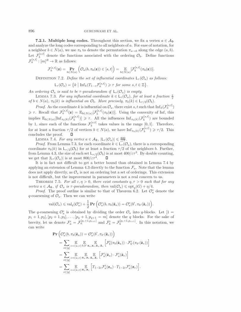
7.2.1. Multiple long codes. Throughout this section, we fix a vertex a ∈ AΦ
and analyze the long codes corresponding to all neighbors of a. For ease of notation, fora neighbor b ∈ N(a), we use πb to denote the permutation πa→b along the edge (a, b).
Let F [s,t]b denote the functions associated with the ordering Ob. Define functions
F [s,t]a : [m]R → R as follows:
F [s,t]a (z) = Pr
b∈N(a)
(Oa(b, πb(z)) ∈ [s, t]
)= E
b∈N(a)[F [s,t]
b (πb(z))].
Definition 7.2. Define the set of influential coordinates Lτ (Oa) as follows:
Lτ (Oa) ={k∣∣ Infk(T1−εF [s,t]
a ) � τ for some s, t ∈ Z}.
An ordering Oa is said to be τ-pseudorandom if Lτ (Oa) is empty.Lemma 7.3. For any influential coordinate k ∈ Lτ (Oa), for at least a fraction τ
2of b ∈ N(a), πb(k) is influential on Ob. More precisely, πb(k) ∈ Lτ/2(Ob).
Proof. As the coordinate k is influential onOa, there exist s, t such that Infk(F [s,t]a )
� τ . Recall that F [s,t]a (z) = Eb∈N(a)[F [s,t]
b (πb(z))]. Using the convexity of Inf, this
implies Eb∈N(a)[Infπb(k)(F[s,t]b )] � τ . All the influences Infπb(k)(F
[s,t]b ) are bounded
by 1, since each of the functions F [s,t]b takes values in the range [0, 1]. Therefore,
for at least a fraction τ/2 of vertices b ∈ N(a), we have Infπb(k)(F[s,t]b ) � τ/2. This
concludes the proof.Lemma 7.4. For any vertex a ∈ AΦ, |Lτ (Oa)| � 800
ετ4 .Proof. From Lemma 7.3, for each coordinate k ∈ Lτ (Oa), there is a corresponding
coordinate πb(k) in Lτ/2(Ob) for at least a fraction τ/2 of the neighbors b. Further,from Lemma 4.3, the size of each set Lτ/2(Ob) is at most 400/ετ3. By double counting,we get that |Lτ (Oa)| is at most 800/ετ4.
It is in fact not difficult to get a better bound than obtained in Lemma 7.4 byapplying an extension of Lemma 4.3 directly to the function Fa. Note that the lemmadoes not apply directly, as Oa is not an ordering but a set of orderings. This extensionis not difficult, but the improvement in parameters is not a real concern to us.
Theorem 7.5. For all ε, η > 0, there exist constants q, τ > 0 such that for anyvertex a ∈ AΦ, if Oa is τ-pseudorandom, then val(Oa) � optq(G) + η/4.
Proof. The proof outline is similar to that of Theorem 6.2. Let O∗a denote the
q-coarsening of Oa. Then we can write
val(Oa) � valq(O∗a) +
1
2Pr(O∗
a(b, πb(zu)) = O∗a(b
′, πb′(zv))).
The q-coarsening O∗a is obtained by dividing the order Oa into q-blocks. Let [1 =
p1 + 1, p2], [p2 + 1, p3], . . . , [pq + 1, pq+1 = m] denote the q blocks. For the sake of
brevity, let us denote F ia = F [pi+1,pi+1]
a and F ib = F [pi+1,pi+1]
b . In this notation, wecan write
Pr(O∗
a(b, πb(zu)) = O∗a(b
′, πb′(zv)))
=∑i∈[q]
Ee=(u,v)
Eb,b′
Ezu,zv ,zu,zv
[F i
b(πb(zu)) · F ib′(πb′ (zv))
]
=∑i∈[q]
Ee=(u,v)
Ezu,zv
Ezu,zv
[F i
a(zu) · F ia(zv)
]
=∑i∈[q]
Ee=(u,v)
Ezu,zv
[T1−2εF i
a(zu) · T1−2εF ia(zv)
].
BEATING THE RANDOM ORDERING IS HARD 897
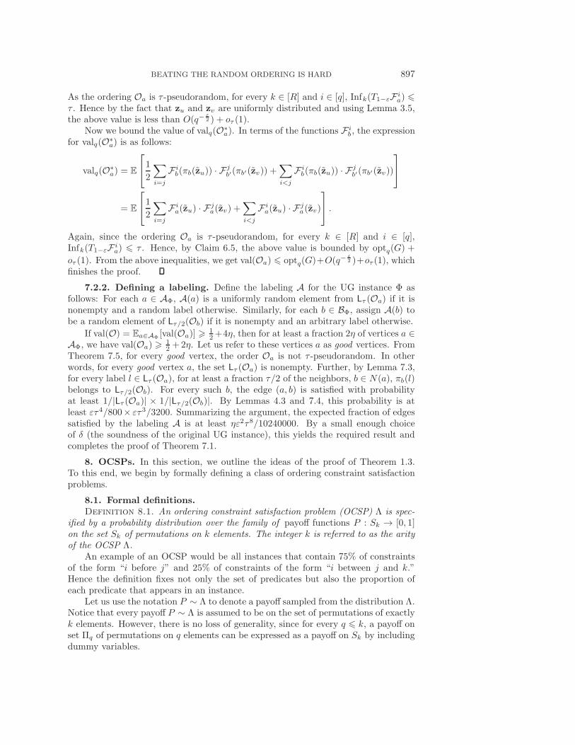
As the ordering Oa is τ -pseudorandom, for every k ∈ [R] and i ∈ [q], Infk(T1−εF ia) �
τ . Hence by the fact that zu and zv are uniformly distributed and using Lemma 3.5,the above value is less than O(q−
ε2 ) + oτ (1).
Now we bound the value of valq(O∗a). In terms of the functions F i
b, the expressionfor valq(O∗
a) is as follows:
valq(O∗a) = E
⎡⎣12
∑i=j
F ib(πb(zu)) · F j
b′(πb′(zv)) +∑i<j
F ib(πb(zu)) · F j
b′(πb′(zv))
⎤⎦
= E
⎡⎣12
∑i=j
F ia(zu) · F j
a(zv) +∑i<j
F ia(zu) · F j
a(zv)
⎤⎦ .
Again, since the ordering Oa is τ -pseudorandom, for every k ∈ [R] and i ∈ [q],Infk(T1−εF i
a) � τ . Hence, by Claim 6.5, the above value is bounded by optq(G) +
oτ (1). From the above inequalities, we get val(Oa) � optq(G)+O(q−ε2 )+oτ (1), which
finishes the proof.
7.2.2. Defining a labeling. Define the labeling A for the UG instance Φ asfollows: For each a ∈ AΦ, A(a) is a uniformly random element from Lτ (Oa) if it isnonempty and a random label otherwise. Similarly, for each b ∈ BΦ, assign A(b) tobe a random element of Lτ/2(Ob) if it is nonempty and an arbitrary label otherwise.
If val(O) = Ea∈AΦ [val(Oa)] � 12+4η, then for at least a fraction 2η of vertices a ∈
AΦ, we have val(Oa) � 12 +2η. Let us refer to these vertices a as good vertices. From
Theorem 7.5, for every good vertex, the order Oa is not τ -pseudorandom. In otherwords, for every good vertex a, the set Lτ (Oa) is nonempty. Further, by Lemma 7.3,for every label l ∈ Lτ (Oa), for at least a fraction τ/2 of the neighbors, b ∈ N(a), πb(l)belongs to Lτ/2(Ob). For every such b, the edge (a, b) is satisfied with probabilityat least 1/|Lτ (Oa)| × 1/|Lτ/2(Ob)|. By Lemmas 4.3 and 7.4, this probability is atleast ετ4/800× ετ3/3200. Summarizing the argument, the expected fraction of edgessatisfied by the labeling A is at least ηε2τ8/10240000. By a small enough choiceof δ (the soundness of the original UG instance), this yields the required result andcompletes the proof of Theorem 7.1.
8. OCSPs. In this section, we outline the ideas of the proof of Theorem 1.3.To this end, we begin by formally defining a class of ordering constraint satisfactionproblems.
8.1. Formal definitions.Definition 8.1. An ordering constraint satisfaction problem (OCSP) Λ is spec-
ified by a probability distribution over the family of payoff functions P : Sk → [0, 1]on the set Sk of permutations on k elements. The integer k is referred to as the arityof the OCSP Λ.
An example of an OCSP would be all instances that contain 75% of constraintsof the form “i before j” and 25% of constraints of the form “i between j and k.”Hence the definition fixes not only the set of predicates but also the proportion ofeach predicate that appears in an instance.
Let us use the notation P ∼ Λ to denote a payoff sampled from the distribution Λ.Notice that every payoff P ∼ Λ is assumed to be on the set of permutations of exactlyk elements. However, there is no loss of generality, since for every q � k, a payoff onset Πq of permutations on q elements can be expressed as a payoff on Sk by includingdummy variables.
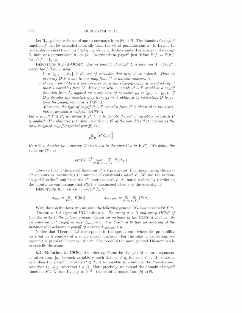
898 GURUSWAMI ET AL.
Let Πk→N denote the set of one-to-one maps from [k] → N. The domain of a payofffunction P can be extended naturally from the set of permutations Sk to Πk→N. Inparticular, an injective map f ∈ Πk→N, along with the standard ordering on the rangeN, induces a permutation πf on [k]. To extend the payoff, just define P (f) = P (πf )for all f ∈ Πk→N.
Definition 8.2 (Λ-OCSP). An instance � of OCSP Λ is given by � = (V ,P),where the following hold:
– V = {y1, . . . , ym} is the set of variables that need to be ordered. Thus anordering O is a one-to-one map from V to natural numbers N.
– P is a probability distribution over constraints/payoffs applied to subsets of atmost k variables from V. More precisely, a sample P ∼ P would be a payofffunction from Λ, applied on a sequence of variables yS = (ys1 , . . . , ysk). IfO|S denotes the injective map from yS → N obtained by restricting O to yS,then the payoff returned is P (O|S).Moreover, the type of payoff P ∼ P sampled from P is identical to the distri-bution associated with the OCSP Λ.
For a payoff P ∈ P, we define V(P ) ⊆ V to denote the set of variables on which Pis applied. The objective is to find an ordering O of the variables that maximizes thetotal weighted payoff/expected payoff, i.e.,
EP∼P
[P (O|P )
].
Here O|P denotes the ordering O restricted to the variables in V(P ). We define thevalue opt(P) as
opt(�) def= max
O:ΠV→N
EP∼P
P (O|P ).
Observe that if the payoff functions P are predicates, then maximizing the pay-off amounts to maximizing the number of constraints satisfied. We use the notions“payoff function” and “constraint” interchangeably. As noted earlier, by reorderingthe inputs, we can assume that P (σ) is maximized when σ is the identity, id.
Definition 8.3. Given an OCSP Λ, let
Λmax = EP∼Λ
[P (id)] , Λrandom = EP∼Λ
Eσ∈Sk
[P (σ)] .
With these definitions, we can state the following general UG-hardness for OCSPs.Theorem 8.4 (general UG-hardness). For every η > 0 and every OCSP of
bounded arity k, the following holds: Given an instance of the OCSP Λ that admitsan ordering with payoff at least Λmax − η, it is UG-hard to find an ordering of theinstance that achieves a payoff of at least Λrandom + η.
Notice that Theorem 1.3 corresponds to the special case where the probabilitydistribution Λ consists of a single payoff function. For the sake of exposition, wepresent the proof of Theorem 1.3 here. The proof of the more general Theorem 8.4 isessentially the same.
8.2. Relation to CSPs. An ordering O can be thought of as an assignmentof values from [m] to each variable yi such that yi = yj for all i = j. By suitablyextending the payoff functions P ∈ Λ, it is possible to eliminate the “one-to-one”condition (yi = yj whenever i = j). More precisely, we extend the domain of payofffunctions P ∈ Λ from Πk→[m] to N
[k]—the set of all maps from [k] to N.
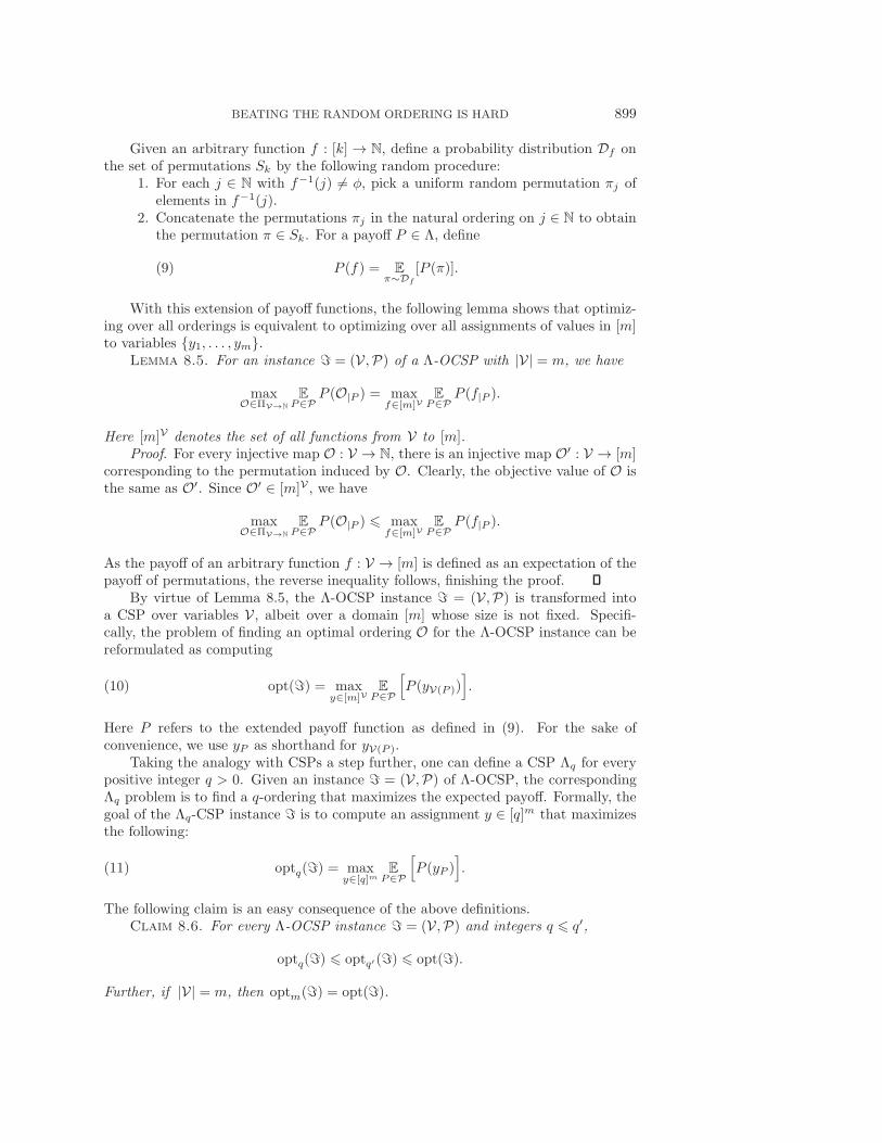
BEATING THE RANDOM ORDERING IS HARD 899
Given an arbitrary function f : [k] → N, define a probability distribution Df onthe set of permutations Sk by the following random procedure:
1. For each j ∈ N with f−1(j) = φ, pick a uniform random permutation πj ofelements in f−1(j).
2. Concatenate the permutations πj in the natural ordering on j ∈ N to obtainthe permutation π ∈ Sk. For a payoff P ∈ Λ, define
(9) P (f) = Eπ∼Df
[P (π)].
With this extension of payoff functions, the following lemma shows that optimiz-ing over all orderings is equivalent to optimizing over all assignments of values in [m]to variables {y1, . . . , ym}.
Lemma 8.5. For an instance � = (V ,P) of a Λ-OCSP with |V| = m, we have
maxO∈ΠV→N
EP∈P
P (O|P ) = maxf∈[m]V
EP∈P
P (f|P ).
Here [m]V denotes the set of all functions from V to [m].Proof. For every injective map O : V → N, there is an injective map O′ : V → [m]
corresponding to the permutation induced by O. Clearly, the objective value of O isthe same as O′. Since O′ ∈ [m]V , we have
maxO∈ΠV→N
EP∈P
P (O|P ) � maxf∈[m]V
EP∈P
P (f|P ).
As the payoff of an arbitrary function f : V → [m] is defined as an expectation of thepayoff of permutations, the reverse inequality follows, finishing the proof.
By virtue of Lemma 8.5, the Λ-OCSP instance � = (V ,P) is transformed intoa CSP over variables V , albeit over a domain [m] whose size is not fixed. Specifi-cally, the problem of finding an optimal ordering O for the Λ-OCSP instance can bereformulated as computing
(10) opt(�) = maxy∈[m]V
EP∈P
[P (yV(P ))
].
Here P refers to the extended payoff function as defined in (9). For the sake ofconvenience, we use yP as shorthand for yV(P ).
Taking the analogy with CSPs a step further, one can define a CSP Λq for everypositive integer q > 0. Given an instance � = (V ,P) of Λ-OCSP, the correspondingΛq problem is to find a q-ordering that maximizes the expected payoff. Formally, thegoal of the Λq-CSP instance � is to compute an assignment y ∈ [q]m that maximizesthe following:
(11) optq(�) = maxy∈[q]m
EP∈P
[P (yP )
].
The following claim is an easy consequence of the above definitions.Claim 8.6. For every Λ-OCSP instance � = (V ,P) and integers q � q′,
optq(�) � optq′ (�) � opt(�).
Further, if |V| = m, then optm(�) = opt(�).
900 GURUSWAMI ET AL.
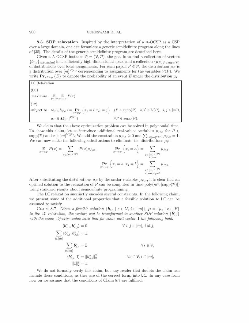
8.3. SDP relaxation. Inspired by the interpretation of a Λ-OCSP as a CSPover a large domain, one can formulate a generic semidefinite program along the linesof [35]. The details of the generic semidefinite program are described here.
Given a Λ-OCSP instance � = (V ,P), the goal is to find a collection of vectors{bi,a}i∈V,a∈[m] in a sufficiently high-dimensional space and a collection {μP }P∈supp(P)
of distributions over local assignments. For each payoff P ∈ P , the distribution μP isa distribution over [m]V(P ) corresponding to assignments for the variables V(P ). Wewrite Prx∈μP {E} to denote the probability of an event E under the distribution μP .
LC Relaxation
maximize EP∼P
Ex∼µP
P (x)
(LC)
subject to 〈bs,i, bs′,j〉 = Prx∼µP
{xs = i, xs′ = j
}(P ∈ supp(P), s, s′ ∈ V(P ), i, j ∈ [m]),
(12)
µP ∈ �([m]V(P )) ∀P ∈ supp(P).
We claim that the above optimization problem can be solved in polynomial time.To show this claim, let us introduce additional real-valued variables μP,x for P ∈supp(P) and x ∈ [m]V (P ). We add the constraints μP,x � 0 and
∑x∈[m]V (P ) μP,x = 1.
We can now make the following substitutions to eliminate the distributions μP :
Ex∼μP
P (x) =∑
x∈[m]V (P )
P (x)μP,x, Prx∼μP
{xi = a
}=
∑x∈[m]V (P )
xi=a
μP,x,
Prx∼μP
{xi = a, xj = b
}=
∑x∈[m]V (P )
xi=a,xj=b
μP,x.
After substituting the distributions μP by the scalar variables μP,x, it is clear that anoptimal solution to the relaxation of P can be computed in time poly(mk, |supp(P)|)using standard results about semidefinite programming.
The LC relaxation succinctly encodes several constraints. In the following claim,we present some of the additional properties that a feasible solution to LC can beassumed to satisfy.
Claim 8.7. Given a feasible solution {bs,i | s ∈ V , i ∈ [m]}, µ = {μe | e ∈ E}to the LC relaxation, the vectors can be transformed to another SDP solution {b∗s,i}with the same objective value such that for some unit vector I the following hold:
〈b∗s,i, b∗s,j〉 = 0 ∀ i, j ∈ [m], i = j,∑i∈[m]
〈b∗s,i, b∗s,i〉 = 1,
∑i∈[m]
b∗s,i = I ∀s ∈ V ,
〈b∗s,i, I〉 = ‖b∗s,i‖22 ∀s ∈ V , i ∈ [m],
‖I‖22 = 1.
We do not formally verify this claim, but any reader that doubts the claim caninclude these conditions, as they are of the correct form, into LC. In any case fromnow on we assume that the conditions of Claim 8.7 are fulfilled.
BEATING THE RANDOM ORDERING IS HARD 901
Note that an integrality gap instance to the above relaxation would be a Λ-OCSPinstance, �, such that sdp(�) is “large” while opt(�) is “small.” A multiscale gapinstance, on the other hand, has much weaker properties—requiring only optq(�)to be small—thus making it easier to construct. Recall Definition 2.3 of multiscalegap instances: An instance � of a Λ-OCSP is a (q, c, s)-multiscale gap instance ifsdp(�) � c and optq(�) � s.
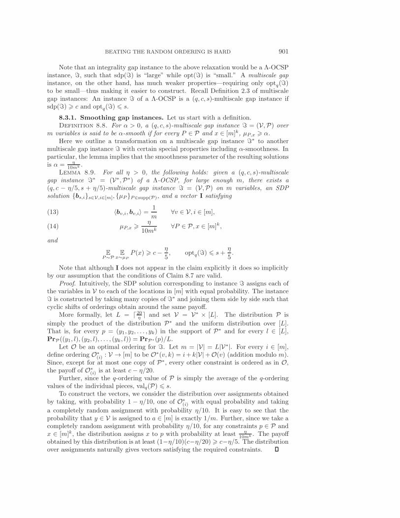
8.3.1. Smoothing gap instances. Let us start with a definition.Definition 8.8. For α > 0, a (q, c, s)-multiscale gap instance � = (V ,P) over
m variables is said to be α-smooth if for every P ∈ P and x ∈ [m]k, μP,x � α.Here we outline a transformation on a multiscale gap instance �∗ to another
multiscale gap instance � with certain special properties including α-smoothness. Inparticular, the lemma implies that the smoothness parameter of the resulting solutionsis α = η
10mk .Lemma 8.9. For all η > 0, the following holds: given a (q, c, s)-multiscale
gap instance �∗ = (V∗,P∗) of a Λ-OCSP, for large enough m, there exists a(q, c − η/5, s + η/5)-multiscale gap instance � = (V ,P) on m variables, an SDPsolution {bs,i}s∈V,i∈[m], {μP }P∈supp(P), and a vector I satisfying
〈bv,i, bv,i〉 =1
m∀v ∈ V , i ∈ [m],(13)
μP,x � η
10mk∀P ∈ P , x ∈ [m]k,(14)
and
EP∼P
Ex∼μP
P (x) � c− η
5, optq(�) � s+
η
5.
Note that although I does not appear in the claim explicitly it does so implicitlyby our assumption that the conditions of Claim 8.7 are valid.
Proof. Intuitively, the SDP solution corresponding to instance � assigns each ofthe variables in V to each of the locations in [m] with equal probability. The instance� is constructed by taking many copies of �∗ and joining them side by side such thatcyclic shifts of orderings obtain around the same payoff.
More formally, let L = � 20η � and set V = V∗ × [L]. The distribution P is
simply the product of the distribution P∗ and the uniform distribution over [L].That is, for every p = (y1, y2, . . . , yk) in the support of P∗ and for every l ∈ [L],PrP((y1, l), (y2, l), . . . , (yk, l)) = PrP∗(p)/L.
Let O be an optimal ordering for �. Let m = |V| = L|V∗|. For every i ∈ [m],define ordering O∗
(i) : V → [m] to be O∗(v, k) = i+ k|V|+O(v) (addition modulo m).Since, except for at most one copy of P∗, every other constraint is ordered as in O,the payoff of O∗
(i) is at least c− η/20.Further, since the q-ordering value of P is simply the average of the q-ordering
values of the individual pieces, valq(P) � s.To construct the vectors, we consider the distribution over assignments obtained
by taking, with probability 1 − η/10, one of O∗(i) with equal probability and taking
a completely random assignment with probability η/10. It is easy to see that theprobability that y ∈ V is assigned to a ∈ [m] is exactly 1/m. Further, since we take acompletely random assignment with probability η/10, for any constraints p ∈ P andx ∈ [m]k, the distribution assigns x to p with probability at least η
10mk . The payoffobtained by this distribution is at least (1−η/10)(c−η/20) � c−η/5. The distributionover assignments naturally gives vectors satisfying the required constraints.
902 GURUSWAMI ET AL.
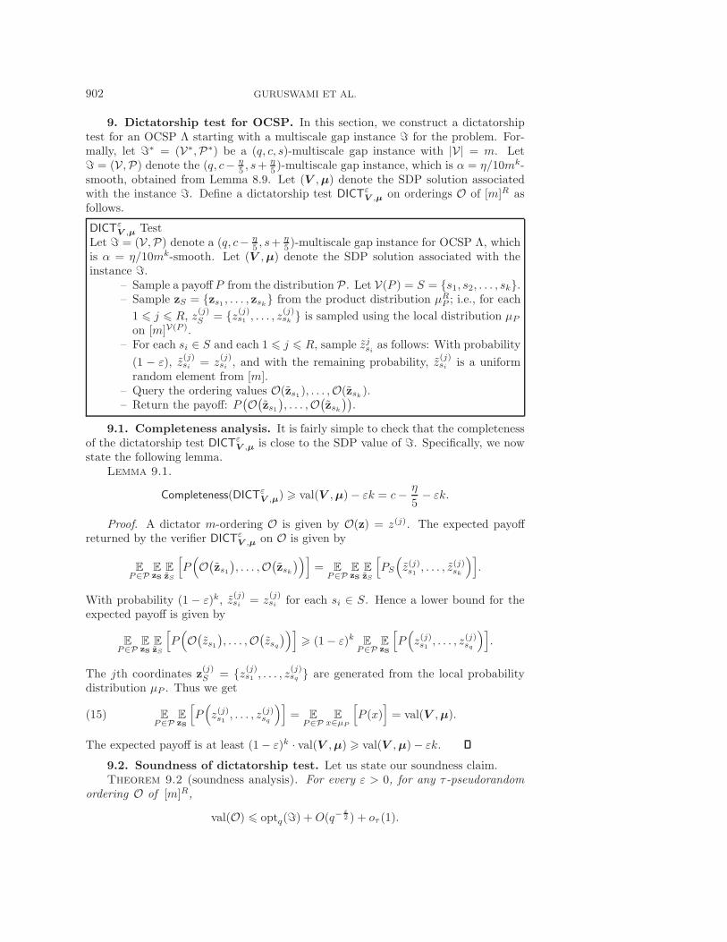
9. Dictatorship test for OCSP. In this section, we construct a dictatorshiptest for an OCSP Λ starting with a multiscale gap instance � for the problem. For-mally, let �∗ = (V∗,P∗) be a (q, c, s)-multiscale gap instance with |V| = m. Let� = (V ,P) denote the (q, c− η
5 , s+η5 )-multiscale gap instance, which is α = η/10mk-
smooth, obtained from Lemma 8.9. Let (V ,µ) denote the SDP solution associatedwith the instance �. Define a dictatorship test DICTε
V ,μ on orderings O of [m]R asfollows.
DICTεV ,μ Test
Let � = (V ,P) denote a (q, c− η5 , s+
η5 )-multiscale gap instance for OCSP Λ, which
is α = η/10mk-smooth. Let (V ,µ) denote the SDP solution associated with theinstance �.
– Sample a payoff P from the distribution P . Let V(P ) = S = {s1, s2, . . . , sk}.– Sample zS = {zs1 , . . . , zsk} from the product distribution μR
P ; i.e., for each
1 � j � R, z(j)S = {z(j)s1 , . . . , z
(j)sk } is sampled using the local distribution μP
on [m]V(P ).– For each si ∈ S and each 1 � j � R, sample zjsi as follows: With probability
(1 − ε), z(j)si = z
(j)si , and with the remaining probability, z
(j)si is a uniform
random element from [m].– Query the ordering values O(zs1 ), . . . ,O(zsk ).– Return the payoff: P
(O(zs1), . . . ,O
(zsk)).
9.1. Completeness analysis. It is fairly simple to check that the completenessof the dictatorship test DICTε
V ,μ is close to the SDP value of �. Specifically, we nowstate the following lemma.
Lemma 9.1.
Completeness(DICTεV ,μ) � val(V ,µ)− εk = c− η
5− εk.
Proof. A dictator m-ordering O is given by O(z) = z(j). The expected payoffreturned by the verifier DICTε
V ,μ on O is given by
EP∈P
EzS
EzS
[P(O(zs1), . . . ,O
(zsk))]
= EP∈P
EzS
EzS
[PS
(z(j)s1 , . . . , z(j)sk
)].
With probability (1 − ε)k, z(j)si = z
(j)si for each si ∈ S. Hence a lower bound for the
expected payoff is given by
EP∈P
EzS
EzS
[P(O(zs1), . . . ,O
(zsq))]
� (1− ε)k EP∈P
EzS
[P(z(j)s1 , . . . , z(j)sq
)].
The jth coordinates z(j)S = {z(j)s1 , . . . , z
(j)sq } are generated from the local probability
distribution μP . Thus we get
(15) EP∈P
EzS
[P(z(j)s1 , . . . , z(j)sq
)]= E
P∈PE
x∈μP
[P (x)
]= val(V ,µ).
The expected payoff is at least (1− ε)k · val(V ,µ) � val(V ,µ)− εk.
9.2. Soundness of dictatorship test. Let us state our soundness claim.Theorem 9.2 (soundness analysis). For every ε > 0, for any τ-pseudorandom
ordering O of [m]R,
val(O) � optq(�) +O(q−ε2 ) + oτ (1).

BEATING THE RANDOM ORDERING IS HARD 903
This theorem is an immediate consequence of Lemmas 9.3 and 9.4, and let usturn to the first of these statements.
Lemma 9.3. For every ε > 0, for any τ-pseudorandom ordering O of [m]R,
val(O) � valq(O∗) +(k
2
)q−
ε2 + oτ (1),
where O∗ is the q-coarsening of O and k denotes the arity of the OCSP Λ.Proof. Let F [s,t] : [m]R → {0, 1} denote the functions associated with the q-
ordering O∗.Note that the loss due to coarsening arises because for some payoffs P the k
variables in V(P ) do not fall into distinct bins during coarsening. Let us upper boundthe probability that some two of the variables queried, zsi and zsj , fall into the sameblock during coarsening, i.e., O∗(zsi ) = O∗(zsj ). Observe that
Pr(O∗(zsi ) = O∗(zsj )
)=∑i∈[q]
EP∈P
Ezsi ,zsj
Ezsi ,zsj
[F i(zsi ) · F i(zsj )
]
=∑i∈[q]
EP∈P
Ezsi ,zsj
[T1−2εF i(zsi ) · T1−2εF i(zsj )
].
As O is a q-coarsening of O, for each value i ∈ [q], there is exactly a fraction 1q of z for
which O∗(z) = i. Hence, for each i ∈ [q], Ez[F i(z) = 1q ]. Further, since the ordering
O∗ is τ -pseudorandom, for every j ∈ [R] and i ∈ [q], Infj(T1−εF i) � τ . Hence, usingLemma 3.5 and the fact that zsi and zsj are uniformly distributed, for sufficientlylarge q, the above probability is bounded by q · q−1− ε
2 + q · oτ (1). By a simple unionbound, the probability that two of the queried values fall in the same bin is at most(k2
)(q · q−1− ε
2 + q · oτ (1)). As all the payoffs are bounded by 1 in absolute value, we
can write
val(O) � valq(O∗) +Pr(∃i, j ∈ [k] such that O∗(zsi) = O∗(zsj )
)� valq(O∗) +
(k
2
)q−
ε2 + oτ (1).
We now state the second lemma needed to prove Theorem 9.2. The proof of thislemma is postponed to section 10.
Lemma 9.4. For every choice of m, q, ε and any τ-pseudorandom q-ordering O∗
of [m]R, valq(O∗) � optq(�) + oτ (1).
10. Soundness analysis for q-orderings. In this section, we give the proofof Lemmas 9.4 and 6.4. As Lemma 6.4 is a special case of Lemma 9.4, we restrictourselves to the proof of Lemma 9.4, which completes the soundness analysis for thedictatorship test for arbitrary OCSPs. The proof of Lemma 9.4 closely resemblesthe soundness analysis of dictatorship tests for the case of generalized CSPs in [35].However, in [35], the dictatorship test is analyzed for functions with domain [q]R andrange �q. In our application, we are interested in functions whose domain is [m]R
while the output is in �q for some q. Hence Lemma 9.4 is not a formal consequenceof the lemmas in [35]. We start with some preliminaries and tools.
10.1. Invariance principle. The following invariance principle is an immediateconsequence of Theorem 3.6 in the work of Isaksson and Mossel [20].
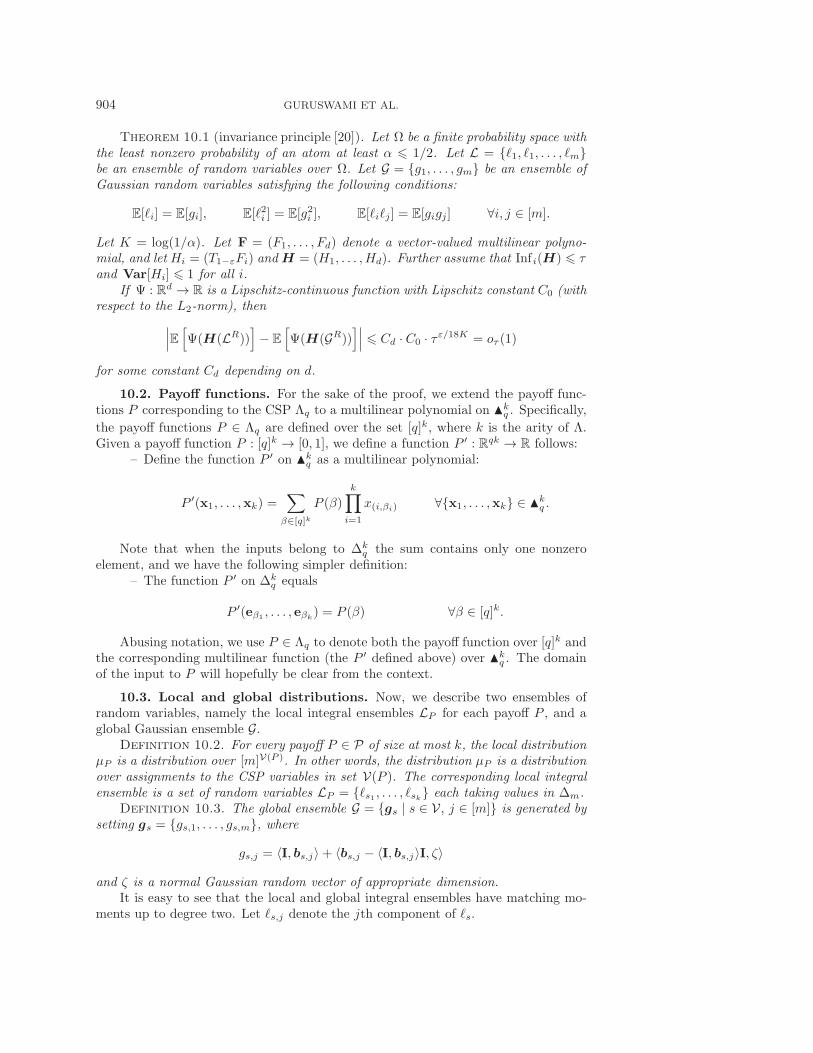
904 GURUSWAMI ET AL.
Theorem 10.1 (invariance principle [20]). Let Ω be a finite probability space withthe least nonzero probability of an atom at least α � 1/2. Let L = {�1, �1, . . . , �m}be an ensemble of random variables over Ω. Let G = {g1, . . . , gm} be an ensemble ofGaussian random variables satisfying the following conditions:
E[�i] = E[gi], E[�2i ] = E[g2i ], E[�i�j] = E[gigj] ∀i, j ∈ [m].
Let K = log(1/α). Let F = (F1, . . . , Fd) denote a vector-valued multilinear polyno-mial, and let Hi = (T1−εFi) and H = (H1, . . . , Hd). Further assume that Infi(H) � τand Var[Hi] � 1 for all i.
If Ψ : Rd → R is a Lipschitz-continuous function with Lipschitz constant C0 (withrespect to the L2-norm), then∣∣∣E [Ψ(H(LR))
]− E
[Ψ(H(GR))
]∣∣∣ � Cd · C0 · τε/18K = oτ (1)
for some constant Cd depending on d.
10.2. Payoff functions. For the sake of the proof, we extend the payoff func-tions P corresponding to the CSP Λq to a multilinear polynomial on �k
q . Specifically,
the payoff functions P ∈ Λq are defined over the set [q]k, where k is the arity of Λ.Given a payoff function P : [q]k → [0, 1], we define a function P ′ : Rqk → R follows:
– Define the function P ′ on �kq as a multilinear polynomial:
P ′(x1, . . . ,xk) =∑
β∈[q]k
P (β)
k∏i=1
x(i,βi) ∀{x1, . . . ,xk} ∈ �kq .
Note that when the inputs belong to Δkq the sum contains only one nonzero
element, and we have the following simpler definition:– The function P ′ on Δk
q equals
P ′(eβ1 , . . . , eβk) = P (β) ∀β ∈ [q]k.
Abusing notation, we use P ∈ Λq to denote both the payoff function over [q]k andthe corresponding multilinear function (the P ′ defined above) over �k
q . The domainof the input to P will hopefully be clear from the context.
10.3. Local and global distributions. Now, we describe two ensembles ofrandom variables, namely the local integral ensembles LP for each payoff P , and aglobal Gaussian ensemble G.
Definition 10.2. For every payoff P ∈ P of size at most k, the local distributionμP is a distribution over [m]V(P ). In other words, the distribution μP is a distributionover assignments to the CSP variables in set V(P ). The corresponding local integralensemble is a set of random variables LP = {�s1 , . . . , �sk} each taking values in Δm.
Definition 10.3. The global ensemble G = {gs | s ∈ V , j ∈ [m]} is generated bysetting gs = {gs,1, . . . , gs,m}, where
gs,j = 〈I, bs,j〉+ 〈bs,j − 〈I, bs,j〉I, ζ〉
and ζ is a normal Gaussian random vector of appropriate dimension.It is easy to see that the local and global integral ensembles have matching mo-
ments up to degree two. Let �s,j denote the jth component of �s.
BEATING THE RANDOM ORDERING IS HARD 905
Lemma 10.4. For any set P ∈ P, the global ensemble G matches the followingmoments of the local integral ensemble LP :
E[gs,j] = E[�s,j ] = 〈I, bs,j〉, E[g2s,j ] = E[�2s,j ] = 〈I, bs,j〉,E[gs,jgs′,j′ ] = E[�s,j�s′,j′ ] = 〈bs,j , bs′,j′ 〉 ∀j, j′, s, s′.
Proof. The statement of the expectations of the expressions involving the �-variables is easy to check. For the expressions involving the g-variables, we need thefact that
E[〈b, ζ〉〈b′, ζ〉] = 〈b, b′〉
and E[〈b, ζ〉] = 0 for any vectors b and b′. The quantity that requires some calculationto compute is E[gs,jgs′,j′ ], which equals
〈I, bs,j〉〈I, bs′,j′〉+ 〈bs,j − 〈I, bs,j〉I, bs′,j′ − 〈I, bs′,j′〉I〉 = 〈bs,j , bs′,j′〉.
Note that local distributions μP for different payoffs P ∈ P do not fit togetherto form a global distribution, and in fact when applying Theorem 10.1 we use thistheorem on each term in the payoff function locally. From this we can conclude thatthe value obtained by the global ensemble on each local condition gives about thesame expected contribution to the objective function as the local distribution specificfor that constraint.
10.4. Putting it all together. Finally, we now show the following lemma,which forms the core of the soundness argument in Lemma 9.4 and is a generalizationof Claim 6.5.
Lemma 10.5. For a function F : [m]R → �q satisfying Infj(T1−εF) � τ for allj ∈ [R],
EP∈P
EzS
EzS
[P(F(zs1), . . . ,F(zsk))] � optq(�) + oτ (1).
Before proving this lemma let us establish Lemma 9.4.Proof of Lemma 9.4. Let F [s,t] : [m]R → {0, 1} denote the functions associated
with the q-ordering O∗. The expected payoff returned by the verifier in the dictator-ship test DICTε
V ,μ is given by
valq(O∗) = EP∈P
EzS
EzS
[P(F(zs1), . . . ,F(zsk))].
Further, since the orderingO∗ is τ -pseudorandom, for every j ∈ [R], we have Infj(T1−εF i)� τ , and thus Lemma 10.5 concludes the proof.
Let us turn to establishing Lemma 10.5.Proof of Lemma 10.5. Let us denote H = T1−εF . Let F(x),H(x) denote the
multilinear polynomials corresponding to functionsF ,H, respectively, where the vari-ables xi,j for i ∈ [R] and j ∈ [m] can be thought of as indicator variables if the jthinput equals i. Let us denote
DICTεV ,μ(F) = E
P∈PEzS
EzS
[P(F(zs1), . . . ,F(zsk))].

906 GURUSWAMI ET AL.
Each vector zsi is independently perturbed to obtain zsi . The payoff functions P aremultilinear when restricted to the domain �q. Consequently, we can write
DICTεV ,μ(F) = E
P∈PEzS
[P(
Ezs1
[F(zs1)|zs1 ], . . . , Ezs1
[F(zsq |zsk ]))]= E
P∈PEzS
[P(H(zs1), . . . ,H(zsk))].
The last equality is due to the fact that Ezsi[F(zsi)|zsi ] = T1−εF(zsi ) = H(zsi). For
each s ∈ S, the coordinates of zs are generated by the distribution μP . Thereforethe above expectation can be written in terms of the polynomial H applied to aninstance of the integral ensemble LP . Specifically, we can write(16)
DICTεV ,μ(F) = E
P∈PEzS
[P(H(zs1), . . . ,H(zsk))] = E
P∈PELR
P
[P(H(�Rs1), . . . ,H
(�Rsk))]
.
The following procedure RoundF returns an ordering for the original Λ-OCSP instance�.RoundF SchemeInput. A Λ-OCSP instance � = (V ,P) with m variables and an SDP solution{bv,i}, {μP}.Truncation Function. Let f� : Rq → �q be a Lipschitz-continuous function suchthat for all x ∈ �q, f�(x) = x. Clearly, a function f� of this nature can beconstructed with a Lipschitz constant Cq depending on q.Scheme. Sample R vectors ζ(1), . . . , ζ(R) with each coordinate being an independentand identically distributed normal random variable.For each v ∈ V do
– For all 1 � j � R and i ∈ [m], compute the projection g(j)v,i of the vector
bv,i as follows:
g(j)v,i = 〈I, bv,i〉+
[〈(bv,i − 〈I, bv,i〉I), ζ(j)〉
].
– Evaluate the function H = T1−εF with g(j)v,i as inputs. In other words,
compute pv = (pv,1, . . . , pv,q) as follows:
pv = H(gv).
– Round pv to p∗v ∈ �q by using the Lipschitz-continuous truncation function
f� : Rq → �q:
p∗v = f�(pv).
– Assign the Λ-OCSP variable v ∈ V the value j ∈ [q] with probability p∗v,j.
Let RoundF (V ,µ) denote the expected payoff of the ordering returned by therounding scheme RoundF on the SDP solution (V ,µ) for the Λ-OCSP instance �.By definition, we have
(17) RoundF (V ,µ) � optq(�).
In the remainder of the proof, we show the following inequality:
RoundF (V ,µ) � DICTεV ,μ(F)− oτ (1).
BEATING THE RANDOM ORDERING IS HARD 907
Along with (17), this would imply that DICTεV ,μ(F) is less than optq(�)+oτ (1), thus
showing the required claim. To this end, we arithmetize the value of RoundF (V ,µ).Notice that the gi are nothing but samples of the global ensemble G associated with �.By definition, the expected payoff is given by
(18) RoundF (V ,µ) = EP∈P
EGRP
[P(f�(H(gR
s1)), . . . , f�
(H(gR
sk)))]
.
We show that the quantities in (16) and (18) are roughly equal. Fix a payoff P ∈ P .Let ΨP : Rqk → R be a Lipschitz-continuous function defined as follows:
ΨP (p1,p2, . . . ,pk) = P(f�(p1
), . . . , f�
(pk
))∀p1, . . . ,pk ∈ �q.
Applying the invariance principle (Theorem 10.1) with the ensembles LP , GP , Lip-schitz-continuous functional Ψ, and the vector of kq multilinear polynomials given by(H ,H, . . . ,H) where H = (H1, . . . , Hq), we get the required result:
RoundF (V ,µ) = EP∈P
EGRP
[ΨP
(H(gRs1
), . . . ,H
(gRsk
))]� E
P∈PELR
P
[ΨP
(H(�Rs1), . . . ,H
(�Rsk))]
− oτ (1)
(∵ invariance principle (Theorem 10.1))
= EP∈P
ELR
P
[P(H(�Rs1), . . . ,H
(�Rsk))]
− oτ (1)
(∵ ΨP (p1, . . . ,pk) = P (p1, . . . ,pk) if ∀i, pi ∈ �q)
= DICTεV ,μ(F)− oτ (1) (∵ (16)).
11. Constructing multiscale gap instances for general OCSP. In thissection, we prove Theorem 11.1, which is the last piece to complete the proof ofTheorem 2.5. We remind the reader that the step moving from the dictator test tothe UG-hardness is completely analogous to the transition done in section 7 for MASand is not presented in this paper.
Theorem 11.1. For every η > 0 and positive integers q, k, there is an m =m(k, q, η) and a distribution, D, over k-tuples of [m] such that the following hold:
– The support of D is contained in the set of strictly increasing k-tuples of [m].– For any f : [m] → [q], let Df denote the distribution over permutations of [m]obtained by extending f as in section 8.2. For any σ = (σ1, σ2, . . . , σk) ∈ Sk,∣∣∣∣ Pr
y∈Df ;(d1,d2,...,dk)∈D[y(dσ1) < y(dσ2) < · · · < y(dσk
)]− 1k!
∣∣∣∣ � η.
Note that the k = 2 case of Theorem 11.1 is the content of Lemma 5.3. Beforedelving into the proof of Theorem 11.1, let us see why it implies a proof of Theorem 2.5.
Proof of Theorem 2.5. Let P be the payoff associated with OCSP Λ, and re-member that it is maximized by the identity permutation. Let m = m(k, q, η/k!),let D be the distribution as promised by Theorem 11.1, and let � = ([m], D) be anOCSP instance with payoff P . Almost by definition, the value obtained by the trivialordering of [m] is the maximal possible P (id). Certainly, the SDP value can be onlyhigher.
908 GURUSWAMI ET AL.
Now, viewing � as an instance of the OCSP Λ, define f to be an optimal q-orderingof �. Then, optq(�) can be bounded as follows:
optq(�) = val(f) = EDEπ∈Df[P (π)] �
∑σ
P (σ)
k!+ η � Λrandom + η.
Let us now turn to the proof of Theorem 11.1.We set m = ks for some integer s to be chosen depending on q and η, and we
think of [m] as the s-tuples of [k], ordered by the lexicographic ordering of the tuples.For an integer r, 0 � r � s, a k-adic interval of order r is an interval of [m] specifiedby an element α ∈ [k]r and denotes the subset of [k]s whose first r coordinates matchthose in α. It is easy to check that for every r and α, such a set is, in fact, an intervalof [m] (due to the lexicographic ordering) and is of length ks−r. For r = 0, it isthe entire set [m], and for r = s, such a set consists of a single element. A randomk-adic interval of order r is a k-adic interval of order r where α is chosen uniformlyat random from [k]r.
Every k-adic interval, I, of order r strictly smaller than s naturally contains kdisjoint k-adic intervals of order r + 1, denoted by I1, I2, . . . , Ik in the order theyappear in I. A random k-adic subinterval, J , is obtained by picking one of these ksubintervals uniformly at random. Let us define our distribution.
Definition 11.2. The distribution Ds is a distribution over k-tuples from [m]for m = ks defined as follows:
1. Pick a random r uniformly in 0 � r � s− 1.2. Pick a random k-adic interval I of order r from [k]s.3. Pick xj uniformly at random from the k-adic subinterval Ij of I, for j =
1, 2, . . . , k.4. Output (x1, x2, . . . , xk).
The first claim of Theorem 11.1 follows immediately from the definition, since theelements chosen are always in increasing order in the lexicographic ordering of [m].
In the rest of this section, we prove that, for the distribution Ds, no functionf : [m] → [q] obtains more than negligible advantage over random with respect to anypermutation π (for large enough s).
Fix a particular function f : [m] → [q]. For p ∈ [q] and an interval I, let μp(I)denote the fraction of I mapped to p by f . The following lemma is the heart of ouranalysis.
Lemma 11.3. For a random k-adic interval I chosen as in Definition 11.2 anda random k-adic subinterval, J , of I, we have
q∑p=1
EI,J
[|μp(I)− μp(J)|
]�√
q
s.
Proof. Let βr,p be E[μp(I)2] when I is a random k-adic interval of order r. Note
first that as E[X ]2 � E[X2] and
μp(I) = EJ [μp(J)],
where the expectation is over a random k-adic subinterval J of I, we have thatβr+1,p � βr,p. Now, for any p ∈ {1, 2, . . . , q}, and a random k-adic interval I of

BEATING THE RANDOM ORDERING IS HARD 909
order r and a random k-adic subinterval J of I,
EI,J
[|μp(I)− μp(J)|
]�(EI,J
[(μp(J)− μp(I))
2])1/2
=
⎛⎝E
I
⎡⎣1k
k∑j=1
(μp(Ij)− μp(I))2
⎤⎦⎞⎠
1/2
=
⎛⎝E
I
⎡⎣ 1k
k∑j=1
μp(Ij)2 − μp(I)
2
⎤⎦⎞⎠
1/2
= (βr+1,p − βr,p)1/2.
Thus, averaging over the choice of random r ∈ {0, 1, . . . , s−1} and summing overall values p in the range [q], we have
q∑p=1
EI,J
[|μp(I)− μp(J)|
]� 1
s
q∑p=1
s−1∑r=0
(βr+1,p − βr,p)1/2
� 1
s
q∑p=1
(s−1∑r=0
1
)1/2(s−1∑r=0
(βr+1,p − βr,p
))1/2
� 1√s
q∑p=1
β1/2s,p �
√q
s
(q−1∑p=1
βs,p
)1/2
=
√q
s.
Next we have the following lemma.
Lemma 11.4. Given nonnegative numbers a(j)i , b
(j)i , i ∈ [q], j ∈ [k], such that for
every j,∑
i a(j)i =
∑i b
(j)i = 1, we have
∑σ∈[q]k
∣∣∣∣∣∣k∏
j=1
a(j)σ(j) −
k∏j=1
b(j)σ(j)
∣∣∣∣∣∣ �k∑
j=1
q∑i=1
∣∣∣ a(j)i − b(j)i
∣∣∣ ,where σ(j) denotes the jth element of the k-tuple σ.
Proof. The proof follows by an induction over k. The two sides of the expressionare equal for k = 1. For k > 1,
∑σ∈[q]k
∣∣∣∣∣∣k∏
j=1
a(j)σ(j) −
k∏j=1
b(j)σ(j)
∣∣∣∣∣∣�∑
σ∈[q]k
⎛⎝∣∣∣∣∣∣a(1)σ(1)
k∏j=2
a(j)σ(j) − a
(1)σ(1)
k∏j=2
b(j)σ(j)
∣∣∣∣∣∣+∣∣∣∣∣∣a(1)σ(1)
k∏j=2
b(j)σ(j) − b
(1)σ(1)
k∏j=2
b(j)σ(j)
∣∣∣∣∣∣⎞⎠
=
⎛⎝∑
i∈[q]
a(1)i
⎞⎠ ·
∑σ∈[q]k−1
∣∣∣∣∣∣k−1∏j=1
a(j+1)σ(j) −
k−1∏j=1
b(j+1)σ(j)
∣∣∣∣∣∣+⎛⎝ k∏
j=2
(q∑
i=1
b(j)i
)⎞⎠ q∑
i=1
∣∣∣a(1)i − b(1)i
∣∣∣
=∑
σ∈[q]k−1
∣∣∣∣∣∣k−1∏j=1
a(j+1)σ(j) −
k−1∏j=1
b(j+1)σ(j)
∣∣∣∣∣∣+q∑
i=1
∣∣∣a(1)i − b(1)i
∣∣∣�
k∑j=2
q∑i=1
∣∣∣a(j)i − b(j)i
∣∣∣+ q∑i=1
∣∣∣a(1)i − b(1)i
∣∣∣ (by induction hypothesis)
=
k∑j=1
q∑i=1
∣∣∣a(j)i − b(j)i
∣∣∣.
910 GURUSWAMI ET AL.
We can now finish the proof of Theorem 11.1 using the above two lemmas. Forany σ ∈ [q]k, let Pr(σ) denote the probability of the event f(xj) = σ(j) when x =(x1, x2, . . . , xk) is chosen according to the distribution Ds. For an interval I, letPr(σ, I) denote the above probability conditioned on Ds choosing I in the secondclaim. Since xj is chosen uniformly from the k-adic subinterval Ij of I, we have
Pr(σ, I) =∏k
j=1 μσ(j)(Ij). Now
∑σ
∣∣∣∣∣∣Pr(σ)− EI
⎡⎣∏
j
μσ(j)(I)
⎤⎦∣∣∣∣∣∣ =∑σ
∣∣∣∣∣∣EI [Pr(σ, I)] − EI
⎡⎣∏
j
μσj (I)
⎤⎦∣∣∣∣∣∣
� EI
⎡⎣∑
σ
∣∣∣∣∣∣Pr(σ, I) −∏j
μσ(j)(I)
∣∣∣∣∣∣⎤⎦
= EI
⎡⎣∑
σ
∣∣∣∣∣∣∏j
μσ(j)(Ij)−∏j
μσ(j)(I)
∣∣∣∣∣∣⎤⎦
� EI
⎡⎣ k∑j=1
∑p∈[q]
∣∣∣μp(Ij)− μp(I)∣∣∣⎤⎦ (by Lemma 11.4)
� k√q/s (by Lemma 11.3).
For any permutation π ∈ Sk, the value of the q-ordering f with respect to π isvalπt (Ds, f) =
∑σ Pr(σ)Payoff
π(σ). Since Payoff takes values in [0, 1], from the aboveargument, ∣∣∣∣∣ valπt (D, f)−
∑σ
Payoffπ(σ)EI
[Πjμσj (I)
] ∣∣∣∣∣ � k√q/s.
Further, since the value of the second factor in terms of the sum depends on whichvalues appear in σ and not their order, the sum is independent of the permutation π,and we get ∣∣valπt (D, f)− 1
k!
∣∣ � k√q/s.
Choosing s greater than k2q/η2, we immediately obtain the statement of Theorem11.1.
Remark 11.5. In Lemma 5.3, we constructed an (η, q)-pseudorandom DAG,which corresponds to the k = 2 case of Theorem 11.1, with n � qO(1/η) vertices. Theabove construction gives an instance of size ks = kO(k2q/η2) which is exp(O(q/η2))for constant k. This is somewhat worse than the size of the DAG construction fromsection 5. But the above construction works for all k, and since we treat q, η asconstants, the exact dependence of the size on these parameters does not matter forour applications.
12. SDP integrality gap. In this section, we construct integrality gaps for theMAS-SDP relaxation using the hardness reduction from UG. Specifically, we showthe following result.
Theorem 12.1. For any γ > 0, there exists a directed graph G such that thevalue of semidefinite program (MAS− SDP) is at least 1− γ, while opt(G) � 1
2 + γ.

BEATING THE RANDOM ORDERING IS HARD 911
The proof uses a bipartite variant of the Khot–Vishnoi UG integrality gap instance[26] as in [35, 29]. Specifically, the following is a direct consequence of [26].
The integrality gap instance Φ = (AΦ ∪ BΦ, E,Π = {πe : [R] → [R] | e ∈ E}, [R])presented in [26] is not bipartite. To obtain a bipartite UG instance Φ′, duplicate thevertices by setting AΦ = {(b, 0) | b ∈ V } and BΦ = {(b, 1) | b ∈ V }. Further, for eachedge (a, b) ∈ E, introduce two edges ((a, 0), (b, 1)) and ((a, 1), (b, 0)) in Φ′. The SDPsolution for the bipartite instance Φ′ is obtained by assigning the vector correspondingto b ∈ V to both vertices (b, 0) and (b, 1). Except for these minor modifications, thefollowing theorem is a direct consequence of [26].
Theorem 12.2 (see [26]). For every δ > 0, there exist a UG instance, Φ =(AΦ ∪ BΦ, E,Π = {πe : [R] → [R] | e ∈ E}, [R]), and vectors {vb,�} for every b ∈ BΦ,� ∈ [R], and a unit vector I such that the following conditions hold:
– No assignment satisfies more than a fraction δ of constraints in Π.– For all b, b′ ∈ BΦ, �, �
′ ∈ [R], 〈vb,�,vb′,�′〉 � 0, and, if � = �′, 〈vb,�,vb,�′〉 = 0.– For all b ∈ BΦ,
∑�∈[R] vb,� = I and 〈vb,�, I〉 = ‖vb,�‖22.
– The SDP value is at least 1−δ: Ea∈AΦ,b,b′∈BΦ
[∑�∈[R]〈vb,πa→b(�),vb′,π′
a→b′(�)〉]
� 1− δ.Proof of Theorem 12.1. Let G be an (η, t)-multiscale gap instance with m vertices.
Apply Theorem 12.2, with a sufficiently small δ, to obtain a UGC instance Φ and SDPvectors {vb,� | b ∈ BΦ, � ∈ [R]}. Consider the instance Ψ constructed by running theUG-hardness reduction in section 7 on the UG instance Φ. The set of vertices of Ψ isgiven by BΦ × [m]R. Set M = |BΦ| ×mR and N = |BΦ|.
The program (MAS − SDP) on the instance Ψ contains M vectors {W(b,z)i |
i ∈ [M ]} for each vertex (b, z) ∈ BΦ × [m]R.Define a solution to (MAS − SDP) as follows: Set the vector I to be the corre-
sponding vector in the instance Φ. For each vertex (b, z) of the graph Ψ, define SDP
vectors {W(b,z)i | i ∈ [M ]} as follows:
W(b,z)i =
{∑z�=i vb,� ∀i ∈ [m], (b, z) ∈ BΦ × [m]R,
0 ∀i /∈ [m].
Now we check that the SDP vectors {W(b,z)i } satisfy conditions (2)–(6) of the MAS-
SDP relaxation.– (Constraint (3)) Since the vectors {vb,�} have a nonnegative dot product, the
vectors {W(b,z)i } have nonnegative inner products too.
– (Constraint (2)) For a fixed b and z, the vectors {W(b,z)i } are constructed by
partitioning the vectors {vb,�} and assigning the vector sum over the parti-
tions. Hence, for any i, j, the vectors W(b,z)i and W
(b,z)j sum over the disjoint
set of �. Thus,
〈W(b,z)i ,W
(b,z)j 〉 =
⟨∑z�=i
vb,�,∑z�′=j
vb,�′
⟩= 0.
– (Constraint (4)) For every vertex (b, z) we have
∑i,j∈[M ]
〈W(b,z)i ,W
(b,z)j 〉 =
∑�,�′∈[R]
〈vb,�,vb,�′〉 =∑�∈[R]
〈vb,�,vb,�〉 = 1.
912 GURUSWAMI ET AL.
– (Constraint (5)) For i /∈ m, we have W(b,z)i = 0, thereby trivially satisfying
constraint (5). For i ∈ [m], we can write
〈I,W(b,z)i 〉 =
∑z�=i
〈I,vb,�〉 =∑z�=i
‖vb,�‖22.
Due to orthogonality of the vectors {vb,i} for every vertex b ∈ BΦ, we get
〈W(b,z)i ,W
(b,z)i 〉 =
⟨∑z�=i
vb,�,∑z�=i
vb,�
⟩=∑z�=i
‖vb,�‖22 = 〈I,W(b,z)i 〉.
– (Constraint (6)) This is satisfied by the choice of I.To prove that the SDP value is close to 1, we first fix a particular choice of a ∈ AΦ,
b, b′ ∈ BΦ. Set π = πa→b, π′ = πa→b′ . The SDP value of edges from (b, ∗) to (b′, ∗) is
Ee∈G
Ezu,zv
∑i<j
〈W(b,π(zu))i ,W
(b′,π′(zv))j 〉 = E
e∈GE
zu,zv
∑i<j
⟨(∑z�u=i
vb,�
),
( ∑z�′v =j
vb′,�′
)⟩
�∑�
(〈vb,π(�),vb′,π′(�)〉) Ee∈G
Przu,zv
[z�u < z�v].
With probability at least (1 − 2ε)2, zu = zu, zv = zv. Further, since the coordinatesof zu, zv are generated from the multiscale gap instance, G, Pr[z�u < z�v] � 1 − η.Hence,
Ee∈G
Ezu,zv
∑i<j
〈W(b,π(zu))i ,W
(b′,π′(zv))j 〉 � (1− 2ε)2(1− η)
∑�
〈vb,π(�),vb′,π′(�)〉.
Thus, the expected payoff over the whole instance is
Ea,b,b′
Ee∈G
Ezu,zv
∑i<j
〈W(b,π(zu))i ,W
(b′,π′(zv))j 〉
� (1− 2ε)2(1− η) Ea∈AΦ,b,b′∈BΦ
∑�
〈vb,π(�),vb′,π′(�)〉
� (1− 2ε)2(1− η)(1 − δ).
Hence, for a sufficiently small choice of parameters ε, η, and δ, the SDP value for Ψis greater than 1− γ. On the other hand, the soundness analysis in section 7 (Theo-rem 7.1) implies that the integral optimum for Ψ is at most 1
2 + γ with a sufficientlysmall choice of ε, η, and δ.
Acknowledgments. We would like to thank Alantha Newman for pointing outthe similarity between MAS and CSPs, and for suggesting the problem. We wouldlike to thank Sanjeev Arora for many fruitful discussions.
REFERENCES
[1] G. Andersson, L. Engebretsen, and J. Hastad, A new way of using semidefinite program-ming with applications to linear equations mod p, J. Algorithms, 39 (2001), pp. 162–204.
[2] P. Austrin, Towards sharp inapproximability for any 2-CSP, SIAM J. Comput., 39 (2010),pp. 2430–2463.
BEATING THE RANDOM ORDERING IS HARD 913
[3] P. Austrin and J. Hastad, Randomly supported independence and resistance, SIAM J. Com-put., 40 (2011), pp. 1–27.
[4] P. Austrin and E. Mossel, Approximation resistant predicates from pairwise independence,Comput. Complexity, 18 (2009), pp. 249–271.
[5] B. Berger and P. W. Shor, Tight bounds for the maximum acyclic subgraph problem, J.Algorithms, 25 (1997), pp. 1–18.
[6] M. Charikar, V. Guruswami, and R. Manokaran, Every permutation CSP of arity 3 isapproximation resistant, in Proceedings of the 24th Annual IEEE Conference on Compu-tational Complexity, 2009, pp. 62–73.
[7] M. Charikar, K. Makarychev, and Y. Makarychev, On the advantage over random formaximum acyclic subgraph, in Proceedings of the 48th Annual IEEE Symposium on Foun-dations of Computer Science, 2007, pp. 625–633.
[8] M. Charikar, Y. Makarychev, and K. Makarychev, Near-optimal algorithms for uniquegames, in Proceedings of the 38th Annual ACM Symposium on Theory of Computing,2006, pp. 205–214.
[9] B. Chor and M. Sudan, A geometric approach to betweenness, SIAM J. Discrete Math., 11(1998), pp. 511–523.
[10] L. Engebretsen and V. Guruswami, Is constraint satisfaction over two variables alwayseasy?, Random Structures Algorithms, 25 (2004), pp. 150–178.
[11] G. Even, J. Naor, B. Schieber, and M. Sudan, Approximating minimum feedback sets andmulticuts in directed graphs, Algorithmica, 20 (1998), pp. 151–174.
[12] U. Feige and M. X. Goemans, Approximating the value of two proper proof systems, with ap-plications to MAX-2SAT and MAX-DICUT, in Proceedings of the Third Israel Symposiumon Theory of Computing and Systems, 1995, pp. 182–189.
[13] M. X. Goemans and D. P. Williamson, Improved approximation algorithms for maximumcut and satisfiability problems using semidefinite programming, J. Assoc. Comput. Mach.,42 (1995), pp. 1115–1145.
[14] V. Guruswami, R. Manokaran, and P. Raghavendra, Beating the random ordering is hard:Inapproximability of maximum acyclic subgraph, in Proceedings of the 49th Annual IEEESymposium on Foundations of Computer Science, 2008, pp. 573–582.
[15] V. Guruswami and Y. Zhou, Approximating Bounded Occurrence Ordering CSPs, manuscript,2010.
[16] G. Hast, Beating a Random Assignment, Ph.D. thesis, Royal Institute of Technology, Stock-holm, Sweden, 2005.
[17] J. Hastad, Some optimal inapproximability results, J. ACM, 48 (2001), pp. 798–859.[18] J. Hastad, Every 2-CSP allows nontrivial approximation, Comput. Complexity, 17 (2008), pp.
549–566.[19] J. Hastad, On the approximation resistance of a random predicate, Comput. Complexity, 18
(2009), pp. 413–434.[20] M. Isaksson and E. Mossel, Maximally stable Gaussian partitions with discrete applications,
Israel J. Math., to appear.[21] A. Karazanov, On the minimal number of arcs of a digraph meeting all its directed cutsets,
Graph Theory Newsletters, 8 (1979).[22] R. M. Karp, Reducibility among combinatorial problems, in Complexity of Computer Compu-
tations, Plenum, New York, 1972, pp. 85–103.[23] S. Khot, On the power of unique 2-prover 1-round games, in Proceedings of the 34th Annual
ACM Symposium on Theory of Computing, 2002, pp. 767–775.[24] S. Khot, G. Kindler, E. Mossel, and R. O’Donnell, Optimal inapproximability results for
MAX-CUT and other 2-variable CSPs?, SIAM J. Comput., 37 (2007), pp. 319–357.[25] S. Khot and O. Regev, Vertex cover might be hard to approximate to within 2-epsilon, J.
Comput. System Sci., 74 (2008), pp. 335–349.[26] S. Khot and N. K. Vishnoi, The Unique Games conjecture, integrality gap for cut problems
and embeddability of negative type metrics into l1, in Proceedings of the 46th Annual IEEESymposium on Foundations of Computer Science, 2005, pp. 53–62.
[27] C. Lucchesi and D. H. Younger, A minimax theorem for directed graphs, J. London Math.Soc. (2), 17 (1978), pp. 369–374.
[28] Y. Makarychev, Simple Linear Time Approximation Algorithm for Betweenness, MicrosoftResearch Technical report MSR-TR-2009-74, 2009.
[29] R. Manokaran, J. S. Naor, P. Raghavendra, and R. Schwartz, SDP gaps and UGChardness for multiway cut, 0-extension and metric labelling, in Proceedings of the 40thACM Symposium on Theory of Computing, 2008, pp. 11–20.
[30] E. Mossel, Gaussian bounds for noise correlation of functions and tight analysis of long codes,

914 GURUSWAMI ET AL.
in Proceedings of the 49th Annual IEEE Symposium on Foundations of Computer Science,2008, pp. 156–165.
[31] E. Mossel, R. O’Donnell, and K. Oleszkiewicz, Noise stability of functions with low influ-ences: Invariance and optimality, Ann. of Math. (2), 171 (2010), pp. 295–341.
[32] A. Newman, Approximating the Maximum Acyclic Subgraph, Master’s thesis, MIT, Cambridge,MA, 2000.
[33] A. Newman, Cuts and orderings: On semidefinite relaxations for the linear ordering problem,in Proceedings of APPROX-RANDOM, 2004, pp. 195–206.
[34] C. H. Papadimitriou and M. Yannakakis, Optimization, approximation, and complexityclasses, J. Comput. System Sci., 43 (1991), pp. 425–440.
[35] P. Raghavendra, Optimal algorithms and inapproximability results for every CSP?, in Pro-ceedings of the 40th ACM Symposium on Theory of Computing, 2008, pp. 245–254.
[36] V. Ramachandran, Finding a minimum feedback arc set in reducible flow graphs, J. Algo-rithms, 9 (1988), pp. 299–313.
[37] P. Seymour, Packing directed circuits fractionally, Combinatorica, 15 (1995), pp. 281–288.[38] U. Zwick, Approximation algorithms for constraint satisfaction problems involving at most
three variables per constraint, in Proceedings of the Ninth Annual ACM-SIAM Symposiumon Discrete Algorithms, 1998, pp. 201–210.