bbaayyeessiiaann aannaallyyssiiss ooff ccllaaiimm rruunn …€¦ · ·...
TRANSCRIPT

BBaayyeessiiaann AAnnaallyyssiiss ooff
CCllaaiimm RRuunn--ooffff TTrriiaanngglleess
KAR WAI LIM
A thesis submitted in partial fulfilment of the requirements for the degree of
Bachelor of Actuarial Studies with Honours in Actuarial Studies
at the Australian National University.
4 November 2011

This thesis contains no material which has been accepted for the award of any
other degree or diploma in any University, and, to the best of my knowledge and
belief, contains no material published or written by another person, except where
due reference is made in the thesis.
...............................................
Kar Wai Lim
4 November 2011

i
Acknowledgements
I would like to express my deepest gratitude to my supervisor, Dr. Borek Puza, who has
given me much support and inspiration. My thesis would not be as refined without his
suggestions for improvement.
I would like to thank my parents, for providing the financial and moral support for my
studies in the ANU. Without this support, I would not be able to study at this prestigious
university. I would also like to thank the College of Business and Economics, for
relieving my parents‟ financial burden by way of a scholarship.
Finally, I appreciate the moral support of all my friends.

ii
Abstract
This dissertation studies Markov chain Monte Carlo (MCMC) methods, and applies
them to actuarial data, with a focus on claim run-off triangles. After reviewing a
classical model for run-off triangles proposed by Hertig (1985) and improved by
de Jong (2004), who incorporated a correlation structure, a Bayesian analogue is
developed to model an actuarial dataset, with a view to estimating the total outstanding
claim liabilities (also known as the required reserve). MCMC methods are used to solve
the Bayesian model, estimate its parameters, make predictions, and assess the model
itself. The resulting estimate of reserve is compared to estimates obtained using other
methods, such as the chain-ladder method, a Bayesian over-dispersed Poisson model,
and the classical development correlation model of de Jong.
The thesis demonstrates that the proposed Bayesian correlation model performs well for
claim reserving purposes. This model yields similar results to its classical counterparts,
with relatively conservative point estimates. It also gives a better idea of the
uncertainties involved in the estimation procedure.

iii
Table of Contents
CHAPTER 1 Introduction ........................................................................................... 1
CHAPTER 2 Bayesian Inference and MCMC Methods ........................................... 4
2.1 Bayesian modelling ................................................................................................ 4
2.2 Markov chain Monte Carlo methods ...................................................................... 5
2.3 MCMC inference .................................................................................................... 9
2.4 WinBUGS ............................................................................................................. 11
2.5 Application of MCMC methods to time series..................................................... 11
2.5.1 Underlying model and data ............................................................................ 11
2.5.2 Priors and the joint posterior distribution ...................................................... 12
2.5.3 A Metropolis-Hastings algorithm ................................................................. 14
2.5.4 Inference on marginal posterior densities ...................................................... 16
2.5.5 Predictive inference ....................................................................................... 19
2.5.6 Hypothesis testing .......................................................................................... 23
2.5.7 Assessment of the MCMC estimates ............................................................. 24
2.5.8 WinBUGS implementation of the MCMC methods ...................................... 28
CHAPTER 3 Claim Run-off Triangles and Data .................................................... 31
3.1 Claim run-off triangles ......................................................................................... 31
3.2 The AFG data ....................................................................................................... 31
CHAPTER 4 Bayesian Modelling of the AFG Data ................................................ 34
4.1 Reserving methods ............................................................................................... 34
4.2 Bayesian models ................................................................................................... 35
CHAPTER 5 Analysis and Results ............................................................................ 39
5.1 Hertig‟s model ...................................................................................................... 39
5.2 A modified Hertig‟s model ................................................................................... 45
5.3 Development correlation model ........................................................................... 50

iv
CHAPTER 6 Model Diagnostics and MCMC Assessment ..................................... 56
6.1 Hypothesis testing ................................................................................................ 56
6.1.1 Hertig‟s model ............................................................................................... 61
6.1.2 Modified Hertig‟s model ............................................................................... 62
6.1.3 Development correlation model .................................................................... 63
6.2 Reserve assessment .............................................................................................. 64
CHAPTER 7 Comparison to Previous Studies ........................................................ 71
CHAPTER 8 Summary and Discussion .................................................................... 73
8.1 Limitations of the Bayesian development correlation model ............................... 73
8.2 Suggestions for future research ............................................................................ 74
8.3 Conclusion ............................................................................................................ 74
Bibliography ............................................................................................................... 76
Appendix ............................................................................................................... 79
Appendix A: Derivations and proofs .......................................................................... 79
Appendix B: R code ................................................................................................... 83
Appendix C: WinBUGS Code .................................................................................... 92
Appendix D: Additional tables and figures .............................................................. 100
v
List of Figures
Figure 2.1: Simulated time series values of ................................................................ 12
Figure 2.2: Trace of .................................................................................................... 15
Figure 2.3: Trace of .................................................................................................... 15
Figure 2.4: Trace of .................................................................................................. 16
Figure 2.5: Frequency histogram of simulated .......................................................... 18
Figure 2.6: Frequency histogram of simulated .......................................................... 18
Figure 2.7: Frequency histogram of simulated ......................................................... 19
Figure 2.8: Estimated posterior mean of future values ............................................... 20
Figure 2.9: Rao-Blackwell posterior mean of future values ....................................... 22
Figure 2.10: Frequency histogram of
.................................................................. 23
Figure 2.11: Approximated exact marginal posterior density of ................................ 26
Figure 2.12: Approximated exact marginal posterior density of ................................ 26
Figure 2.13: Approximated exact marginal posterior density of .............................. 27
Figure 5.1: Trace of simulated .................................................................................. 42
Figure 5.2: Trace of simulated .................................................................................. 42
Figure 5.3: Trace of simulated .................................................................................. 42
Figure 5.4: Trace for simulated values of reserve (modified Hertig‟s model) .............. 49
Figure 5.5: Trace of ................................................................................................... 53
Figure 5.6: Trace of ................................................................................................... 53
Figure 5.7: Trace of ................................................................................................... 53
Figure 5.8: Trace of simulated reserve ........................................................................ 55
Figure 6.1: Frequency histogram of simulated reserve .................................................. 68
Figure 8.1: Frequency histogram of simulated ......................................................... 100
Figure 8.2: Frequency histogram of simulated ....................................................... 100
Figure 8.3: Traces of simulated , and (Hertig‟s model) ................................. 101
Figure 8.4: Traces of simulated , , , and (modified Hertig‟s model) ....... 103
Figure 8.5: Traces of simulated , , , , and (dev. corr. model) ............... 103
Figure 8.6: Simulated values of vs simulated values of ..................................... 104

vi
List of Tables
Table 2.1: Estimated posterior quantities (R output) ..................................................... 17
Table 2.2: Predictive inference on future values (R output) ....................................... 20
Table 2.3: Rao-Blackwell estimates of posterior mean of future values .................... 21
Table 2.4: Estimated posterior quantities (WinBUGS output) ....................................... 29
Table 2.5: Predictive inference of future values (WinBUGS output) .......................... 29
Table 3.1: AFG data - cumulative incurred claim amounts ...................................... 32
Table 3.2: AFG data - exact incurred claim amounts .................................................... 33
Table 4.1: AFG data - development factors ............................................................. 36
Table 5.1: Posterior estimates of , and (Hertig‟s model) .................................. 40
Table 5.2: Predictive inference on the future (Hertig‟s model) ................................ 44
Table 5.3: Predictive inference on reserve (Hertig‟s model) ......................................... 45
Table 5.4: Posterior estimates of , , , and (modified Hertig‟s model) ........ 47
Table 5.5: Predictive inference on future and (modified Hertig‟s model) ............. 48
Table 5.6: Posterior estimates (development correlation model) ................................... 52
Table 5.7: Predictive inference on and (development correlation model) ............. 54
Table 6.1: AFG data – ............................................................................................ 59
Table 6.2: Posterior predictive p-values (Hertig‟s model) ............................................. 61
Table 6.3: Posterior predictive p-values (modified Hertig‟s model) ............................. 62
Table 6.4: Posterior predictive p-values (development correlation model) ................... 63
Table 6.5: Simulated data - cumulative incurred claim amounts ............................. 67
Table 7.1: Forecasted liabilities for the AFG data .............................................. 71
Table 8.1: Predictive inference on cumulative claim liabilities and reserve ................ 102

1
CHAPTER 1
IInnttrroodduuccttiioonn
Markov chain Monte Carlo (MCMC) methods play an important role in Bayesian
statistics, especially when inference cannot be made directly due to the complexity of
the Bayesian model, for example, when there is no closed form solution to the posterior
distribution of a target parameter. MCMC methods allow one to sample random values
from the posterior distribution; these values are subsequently used to estimate quantities
of interest, such as the posterior means of model parameters. MCMC methods are often
easy and quick to implement, and provide an alternative approach to the analysis of
Bayesian models even when an analytic solution is possible.
This thesis demonstrates the usefulness of MCMC methods when applied to the
Bayesian analysis of actuarial data, with a focus on claim run-off triangles. A
run-off triangle shows the claim liabilities for accidents occurring in certain years
and the delays in claim reporting. Traditionally, deterministic algorithms such as the
chain-ladder (CL) method (Harnek, 1966) and the Bornhuetter-Ferguson method
(Bornhuetter & Ferguson, 1972) were used to forecast the future claim liabilities to
determine the outstanding claims reserve. With improvement in technology and the
need to identify the variability underlying the future claim liabilities, stochastic models
were developed and analysed to justify these deterministic algorithms; the most notable
of these stochastic models is the stochastic CL method developed by Mack (1993). A
summary of the stochastic CL method can be found in Mack (2006). An extensive
literature on claims reserving is available in the book by Taylor (2000).
1. Introduction
2
Several Bayesian models for claim run-off triangles were considered by Verrall (1990),
de Alba (2002, 2006), England & Verrall (2002), Lamps (2002a, 2002b, 2002c),
Scollnik (2004), de Alba & Nieto-Barajas (2008), England, Verrall, & Wuthrich (2010)
and other researchers. Verrall (1990) analysed the traditional CL method using the
theory of Bayesian linear models, by transforming the multiplicative CL model into
linear model by taking logarithms. Verrall utilises a Kalman filter (state space) approach
in the Bayesian analysis. de Alba (2002, 2006) presented Bayesian approach for several
models using direct Monte Carlo (MC) method. England and Verrall (2002) proposed
a Bayesian analysis using an over-dispersed Poisson CL model, they compared
and contrasted this approach with other reserving methods. Details on the Bayesian
over-dispersed Poisson model are available in England et al. (2010). Lamps (2002a,
2002b, 2002c) discussed various MCMC models to deal with claim run-off triangles,
and Scollnik (2004) performed MCMC methods on the CL model using statistical
package WinBUGS (to be discussed further in Chapter 2). As mentioned in Scollnik
(2004), the Bayesian approach is useful because Bayesian models allow prior
information to be included in the analysis, if available. Bayesian models allow
parameter uncertainty and model uncertainty to be incorporated in the analysis and
predictive inference. They also yield complete posterior distributions for quantities of
interest rather than just point estimates and confidence intervals.
This thesis considers the Bayesian analogue of a frequentist (classical) model proposed
by de Jong (2004), which in turn is an extension of a model proposed by Hertig (1985).
Hertig‟s model is different from all the models mentioned in the previous paragraph
because it models the log-link ratios of the cumulative liabilities instead of the claim
liabilities directly. de Jong extended Hertig‟s model by introducing a correlation

1. Introduction
3
structure. These models of Hertig and de Jong will be discussed further in Chapter 4.
This thesis contributes to the existing literature by developing a Bayesian model for
de Jong‟s classical model and comparing the two. MCMC methods will be used to
perform the Bayesian analysis.
The next chapter provides an overview of the Bayesian approach and MCMC methods
generally. Chapter 3 describes claim run-off triangles, in particular the data to be
analysed. In Chapter 4, the classical models proposed by Hertig (1985) and
de Jong (2004) are studied and Bayesian analogues thereof are developed. Chapter 5
discusses how MCMC methods can be used to perform the Bayesian analysis; the
results of the analysis are then presented. Chapter 6 assesses the Bayesian models in
terms of goodness-of-fit and the appropriateness of the estimated reserve. Comparison
of the Bayesian results with those of previous studies is made in Chapter 7. Finally,
Chapter 8 provides a summary of the thesis, discusses limitations of the approach taken
and suggests several avenues for further research.

4
CHAPTER 2
BBaayyeessiiaann IInnffeerreennccee aanndd MMCCMMCC MMeetthhooddss
2.1 Bayesian modelling
A classical model treats its unknown parameters as constants that need to be estimated,
whereas a Bayesian model regards the same parameters as random variables, each of
them having a prior distribution. It is assumed that the readers of the thesis understand
the basics of Bayesian methods and hence discussion will focus on Bayesian inference
and results. Readers may find the introductory text “Bayesian Data Analysis” by
Gelman, Carlin, Stern, and Rubin (2003) useful. Important formulae, results and
examples will now be presented as a brief overview of Bayesian methods.
Consider the following Bayesian model:
where denotes the probability density function (pdf).
In this Bayesian model, the joint posterior density of and can be written as
where and
.
It is often convenient to write the joint posterior density up to a proportionality constant,
namely since can be hard to determine and does not

2. Bayesian Inference and MCMC Methods
5
depend on and (the arguments in ). The marginal posterior densities can
be derived by integrating out the relevant nuisance parameter, in this case:
These integrals are usually difficult to express in closed form when the model is
complicated or there are many parameters (note that and are possibly vectors).
Hence inference on and may be impractical, if not impossible; one may then
consider approximating the solutions of the equations involved using special techniques
such as numerical integration. However, these can be tedious and time consuming.
2.2 Markov chain Monte Carlo methods
MCMC methods are useful because they can provide simple but typically very good
approximations to integrals and other equations that are very difficult or impossible to
obtain directly. With these methods, knowing only the joint posterior density,
(up to a proportionality constant) is sufficient for inference to be made on the marginal
posterior densities, and . Briefly, this is achieved by alternately
simulating random observations from the conditional marginal posterior densities,
and (each of which is proportional to the joint posterior density,
), so as to ultimately produce random samples (as detailed below) from
the (unconditional) marginal posterior densities, and . Estimates of
and can then be obtained from these latter samples. Moreover, these samples
can also be used to estimate any, possibly very complicated, functions of and
e.g. .

2. Bayesian Inference and MCMC Methods
6
MCMC methods were first proposed by Metropolis et al. (1953), and subsequently
generalised by Hastings (1970), leading to the Metropolis-Hastings (MH) algorithm.
The MH algorithm can be summarised as follows:
i. Specify an initial value for , call it , which will be the starting point
for the algorithm‟s simulation process.
ii. Define driver distributions for the parameters and from which the next
simulated values will be sampled. Let the pdfs of the driver distributions for and
be and , respectively.
iii. Sample a candidate value of from call it and accept it with
probability
Then the value of is updated to be if is accepted. Otherwise,
retains the previous value, i.e. .
To decide whether is accepted, generate . Then accept if
. (Note that is automatically accepted if .)
iv. Sample a candidate value of from call it , and accept it with
probability
Then the value of is updated to be if is accepted. Otherwise, retains
the previous value, i.e. . To decide whether is accepted, generate
. Then accept if . This concludes the first iteration.

2. Bayesian Inference and MCMC Methods
7
v. Repeat steps iii and iv again and again until a desired total large sample of size
is created, i.e. . This concludes the MH algorithm.
vi. Decide on a suitable burn-in length (see below). Next, relabel as
and as . Then take as an
approximately iid sample from .
A drawback of the MH algorithm is that the simulated values are not truly independent
(hence the word „approximate‟ in step vi above); their correlation comes from the
Markov chain method where the next simulated value is obtained from its predecessor.
Also, a bad choice of initial values distorts the sampling distribution. This means that a
truly random sample of the posterior density is not available. Fortunately, the simulated
values converge to their marginal posterior density as the number of iterations, gets
larger. Hence, these problems with MCMC methods can be addressed by setting to be
very large, say , and discarding the initial portion of the simulated data, for
example, a burn-in of , for a final sample of size .
The theory of convergence and how to choose and will not be discussed in the
thesis; refer to Raftery & Lewis (1995) for details regarding these issues. To ensure a
good mixing of the simulated values, where and as a whole represent the true
marginal posterior distributions and each and is a random realisation from the
distributions, a conservative approach will be used in choosing the number of
simulations and burn-in . Convergence can then be assessed from the traces of the
algorithm, which show the time series values of simulated and ; a cut-off point can
then be chosen conservatively for a suitable burn-in.

2. Bayesian Inference and MCMC Methods
8
The driver distributions are usually chosen so that the candidate values will be easy to
sample from; examples include the uniform and normal distributions. A suitable choice
of driver distribution allows the candidate values to be accepted more frequently with
higher probability of acceptance, which is desirable as the algorithm produces a better
mixing of simulated values with lower wastage (rejections of and ).
Note that when a driver distribution is chosen to be a symmetric distribution, in the
sense that and the acceptance
probabilities simplify to
and
The MH algorithm reduces to the Gibbs sampler when the driver distributions are
chosen to be the conditional posterior distributions, i.e. when is set to be
and is set equal to . In this case, the acceptance
probability for reduces to
and likewise reduces to .
The Gibbs sampler is preferred to the general MH algorithm because it produces no
wastage. However, sometimes a considerable amount of effort is needed to derive the
distribution of the conditional density and/or to sample from it. Thus there may be a
trade-off between efficiency and simplicity.

2. Bayesian Inference and MCMC Methods
9
2.3 MCMC inference
From a large sample with appropriate burn-in, the simulated values of and can be
used to make inferences on and , as well as on any function of and . For example,
one may wish to estimate by its posterior mean, , but this involves solving
a difficult or impossible integral to determine the posterior mean. Therefore, in turn, is
estimated by the Monte Carlo sample mean, .
This estimate is unbiased because
since
With the aid of a statistical package such as S-Plus or R, the entire marginal posterior
distributions can also be estimated from the simulated values. The estimated
marginal posterior distributions can then be displayed on a graph as a representation
of the true marginal posterior distributions. The approximation improves with the
number of simulations. This provides a simple alternative to deriving the exact
distributions analytically, typically by integration. Inference on functions of and
such as mentioned above, can be performed in a similar manner; this is
achieved simply by calculating values and applying the method of
Monte Carlo, as before. (i.e. to estimate by ).
MCMC methods also allow predictive inference to be made in a convenient manner,
when one is interested in some quantity for which is known. For instance,
could be a future independent replicate of in which case is the same as
with changed to .

2. Bayesian Inference and MCMC Methods
10
Then the predictive density is
Usually it is difficult to derive the predictive density analytically. However,
observations of the predictive quantity can often be sampled easily from the predictive
distribution using the method of composition. This is done by sampling from
where and are taken from the MCMC sample described above. The
triplet is then a sample value from ; also, is a random
observation from . Thus, inference on , or any function of , and , can be
performed much more conveniently without deriving the predictive density directly.
There are two general approaches to obtaining a Bayesian estimate of a general quantity
of interest using a MCMC sample. First there is the „normal method‟ (as mentioned
above) whereby the posterior mean of the quantity, is estimated by
the respective MCMC sample mean, ; e.g. if then is estimated
by .
Alternatively, one may apply the
„Rao-Blackwell method‟ (see McKeague & Wefelmeyer, 2000) and estimate by the
sample mean of a conditional posterior expected value of . An example of the
Rao-Blackwell method is shown below in Subsection 2.5.5. This method is often more
precise than the normal method; however, it is typically more complicated and requires
further derivations.
In addition to using the mean for predictive inference, one could also consider the
median and mode. Comparing these statistics may give an idea of the underlying
distribution of the quantity of interest, . In Bayesian decision theory, the mean

2. Bayesian Inference and MCMC Methods
11
minimises the quadratic error loss function, the median minimises the absolute error
loss function and the mode minimises the zero-one error loss function. An actuary may
need to consider, in his or her application, the costs associated with making errors of
various magnitudes. In practice, the quadratic error loss function is usually chosen.
2.4 WinBUGS
WinBUGS (Bayesian inference Using Gibbs Sampling for Windows) is a software
package which is useful for analysing Bayesian models via MCMC methods
(Lunn, Thomas, Best, & Spiegelhalter, 2000). This software utilises the Gibbs sampler
to produce the simulated values. Using WinBUGS to estimate the quantities of interest
is much quicker and simpler than writing the algorithm codes manually (e.g. in S-plus
or R). This is because Gibbs sampling is done internally by WinBUGS without the need
to derive the posterior distribution of the parameters. Refer to Sheu & O‟Curry (1998)
and Merkle & Zandt (2005) for an introduction to WinBUGS.
2.5 Application of MCMC methods to time series
In the following example, MCMC methods are used to analyse a randomly generated
time series data with statistical package R. This is done by coding the MH algorithm
in R. MCMC simulations are also performed using WinBUGS at the end of the section
for comparison purpose.
2.5.1 Underlying model and data
Consider the following stationary AR(1) model (autoregressive model of order 1):
2. Bayesian Inference and MCMC Methods
12
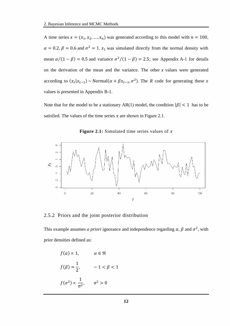
A time series was generated according to this model with
and . was simulated directly from the normal density with
mean and variance ; see Appendix A-1 for details
on the derivation of the mean and the variance. The other values were generated
according to . The R code for generating these
values is presented in Appendix B-1.
Note that for the model to be a stationary AR(1) model, the condition has to be
satisfied. The values of the time series are shown in Figure 2.1.
Figure 2.1: Simulated time series values of
2.5.2 Priors and the joint posterior distribution
This example assumes a priori ignorance and independence regarding and with
prior densities defined as:
2. Bayesian Inference and MCMC Methods
13
Note that the prior distributions of and are improper, for which their densities do
not integrate to . These priors (including ) are uninformative (or non-informative) in
the sense that they do not provide any real information of their underlying values. Care
should be taken when using improper priors, as they might produce improper posterior
distributions, which are nonsensical for making inferences, see Hobert & Casella (1996)
for a detailed analysis on the dangers of using improper priors. According to
Hobert & Casella, “the fact that it is possible to implement the Gibbs sampler without
checking that the posterior is proper is dangerous”.
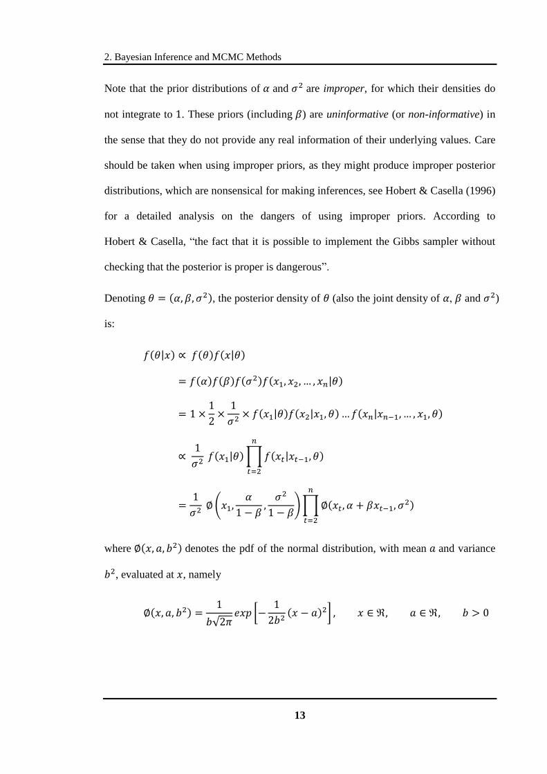
Denoting , the posterior density of (also the joint density of and )
is:
where denotes the pdf of the normal distribution, with mean and variance
, evaluated at , namely

2. Bayesian Inference and MCMC Methods
14
Deriving the marginal posterior densities from the joint posterior density is impractical
given the complex nature of the joint posterior density. Nevertheless, the marginal
posterior density can be estimated via MCMC methods, as detailed in the following
subsections.
2.5.3 A Metropolis-Hastings algorithm
A MH algorithm was designed and implemented (see the R code in Appendix B-2) so as
to generate a sample of values of with symmetric uniform drivers. The mean of
the driver distributions were chosen to be the last simulated values of , with starting
points , and . Specifically, the driver distributions are:
where , and are called the tuning parameters.
The acceptance rates were found to be for , for and for .
(For example, of the proposed values of were accepted.) In the
algorithm, the values of were restricted between and , while the values of
were restricted to be positive. Figure 2.2, 2.3 and 2.4 show the traces of the sampling
process. These are plots of the simulated values; the dotted lines show the cut-off point
for burn-in, . These figures show that the simulated values of , and
converge very quickly and exhibit a good mixing.

2. Bayesian Inference and MCMC Methods
15
Figure 2.2: Trace of
Figure 2.3: Trace of

2. Bayesian Inference and MCMC Methods
16
Figure 2.4: Trace of
2.5.4 Inference on marginal posterior densities
After burn-in, the simulated values of and can be thought of being
sampled directly from the marginal posterior densities. This allows inference on
the marginal posterior densities to be made from these simulated values. Table 2.1
shows the estimates of the posterior mean of (alpha), (beta), (sigma^2),
(eta) and (tau^2), together with
their 95% confidence intervals (CI) and 95% central posterior density regions (CPDR).
The first CI is obtained via the „ordinary‟ method which assumes no autocorrelations,
while the second CI is the batch means confidence interval (see Pawlikowski, 1990).
The batch means CI is better since the simulated values generated via MH algorithm are
correlated with varying degree, depending on the driver distributions used. The true
2. Bayesian Inference and MCMC Methods
17
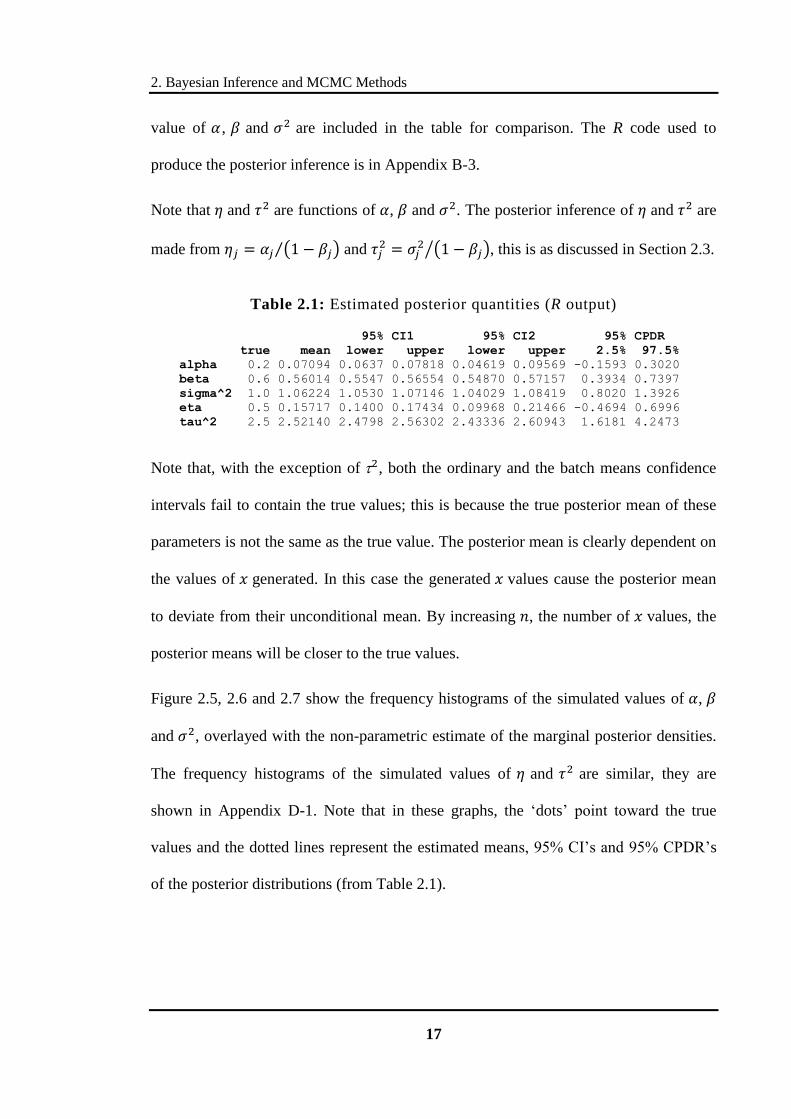
value of , and are included in the table for comparison. The R code used to
produce the posterior inference is in Appendix B-3.
Note that and are functions of , and . The posterior inference of and are
made from and
, this is as discussed in Section 2.3.
Table 2.1: Estimated posterior quantities (R output)
95% CI1 95% CI2 95% CPDR
true mean lower upper lower upper 2.5% 97.5%
alpha 0.2 0.07094 0.0637 0.07818 0.04619 0.09569 -0.1593 0.3020
beta 0.6 0.56014 0.5547 0.56554 0.54870 0.57157 0.3934 0.7397
sigma^2 1.0 1.06224 1.0530 1.07146 1.04029 1.08419 0.8020 1.3926
eta 0.5 0.15717 0.1400 0.17434 0.09968 0.21466 -0.4694 0.6996
tau^2 2.5 2.52140 2.4798 2.56302 2.43336 2.60943 1.6181 4.2473
Note that, with the exception of , both the ordinary and the batch means confidence
intervals fail to contain the true values; this is because the true posterior mean of these
parameters is not the same as the true value. The posterior mean is clearly dependent on
the values of generated. In this case the generated values cause the posterior mean
to deviate from their unconditional mean. By increasing , the number of values, the
posterior means will be closer to the true values.
Figure 2.5, 2.6 and 2.7 show the frequency histograms of the simulated values of ,
and , overlayed with the non-parametric estimate of the marginal posterior densities.
The frequency histograms of the simulated values of and are similar, they are
shown in Appendix D-1. Note that in these graphs, the „dots‟ point toward the true
values and the dotted lines represent the estimated means 95% CI‟s and 95% CPDR‟s
of the posterior distributions (from Table 2.1).

2. Bayesian Inference and MCMC Methods
18
Figure 2.5: Frequency histogram of simulated
Figure 2.6: Frequency histogram of simulated

2. Bayesian Inference and MCMC Methods
19
Figure 2.7: Frequency histogram of simulated
2.5.5 Predictive inference
From the simulated values of , future values can be forecasted from
each set of . In this example, the predicted values of are
generated, according to the following distribution:
These generated values of are analysed in the same way as , and ,
giving the predictive inference shown in Table 2.2. The associated sample
variances and batch means variances (labelled s2b) are also included to illustrate
the increasing uncertainties in the prediction as increases. Note that the 95% CPDR

2. Bayesian Inference and MCMC Methods
20
here corresponds to the 95% prediction interval. See the R codes in Appendix B-4 on
how these estimates are obtained.
Table 2.2: Predictive inference on future values (R output)
95% CI1 95% CI2 95% CPDR
mean lower upper lower upper 2.5% 97.5% s2 s2b
x(n+1) -0.4314 -0.4978 -0.3650 -0.48673 -0.3761 -2.46 1.77 1.15 0.796
x(n+2) -0.1810 -0.2556 -0.1064 -0.26380 -0.0983 -2.51 2.20 1.45 1.783
x(n+3) -0.0188 -0.0942 0.0566 -0.08894 0.0514 -2.53 2.29 1.48 1.281
x(n+4) 0.0121 -0.0668 0.0910 -0.08257 0.1067 -2.66 2.47 1.62 2.331
x(n+5) 0.0675 -0.0110 0.1460 -0.02037 0.1553 -2.46 2.62 1.60 2.009
x(n+6) 0.0958 0.0154 0.1763 -0.01799 0.2097 -2.60 2.57 1.68 3.373
x(n+7) 0.1009 0.0229 0.1790 -0.00558 0.2075 -2.40 2.46 1.59 2.954
x(n+8) 0.1457 0.0649 0.2265 0.02825 0.2632 -2.45 2.68 1.70 3.592
x(n+9) 0.1030 0.0252 0.1807 -0.01233 0.2182 -2.39 2.47 1.57 3.460
x(n+10) 0.1512 0.0765 0.2258 0.01836 0.2839 -2.06 2.52 1.45 4.590
The mean of the forecasted future values converges to the estimated posterior mean
of , , as illustrated in Figure 2.8. Note that the 95% CPDR‟s are too wide
to be included, and hence they are omitted.
Figure 2.8: Estimated posterior mean of future values

2. Bayesian Inference and MCMC Methods
21
An alternative method for predicting the future values is through the Rao-Blackwell
approach, as mentioned in Section 2.3. Using this method, the unnecessary variability
which arose from generating values randomly through its distribution is eliminated.
The Rao-Blackwell estimates of the mean of the forecasted values can be calculated
from the following formulae (refer to Appendix A-2 for proof):
where
and
The Rao-Blackwell estimates together with associated 95% CI‟s are shown in Table 2.3.
Note that the 95% CPDR is irrelevant here since the Rao-Blackwell approach aims to
estimate the mean of the future values directly, i.e. the 95% CPDR is not the 95%
prediction interval when Rao-Blackwell method is used.
Table 2.3: Rao-Blackwell estimates of posterior mean of future values
95% CI1 95% CI2
mean lower upper lower upper
x(n+1) -0.4351 -0.4445 -0.4257 -0.4634 -0.40685
x(n+2) -0.1814 -0.1946 -0.1681 -0.2232 -0.13953
x(n+3) -0.0406 -0.0556 -0.0256 -0.0894 0.00814
x(n+4) 0.0392 0.0234 0.0551 -0.0132 0.09166
x(n+5) 0.0855 0.0691 0.1018 0.0310 0.13995
x(n+6) 0.1128 0.0962 0.1295 0.0572 0.16844
x(n+7) 0.1293 0.1124 0.1461 0.0730 0.18558
x(n+8) 0.1393 0.1224 0.1563 0.0826 0.19607
x(n+9) 0.1456 0.1286 0.1626 0.0886 0.20260
x(n+10) 0.1496 0.1325 0.1667 0.0925 0.20673

2. Bayesian Inference and MCMC Methods
22
Again, the estimated mean converges to the estimated posterior mean of
, but in a steadier manner, as opposed to the predictive inference produced
through the „normal approach‟ (see point in Figure 2.8). Rao-Blackwell
estimation is more precise due to the narrower CI‟s produced, as can be seen
in Figure 2.9.
Figure 2.9: Rao-Blackwell posterior mean of future values
Note that the predictive distribution of can be estimated in a similar way as in
Subsection 2.5.4, by plotting frequency histograms of the generated values
. As an
example, the frequency histogram for
is shown in Figure 2.10.

2. Bayesian Inference and MCMC Methods
23
Figure 2.10: Frequency histogram of
2.5.6 Hypothesis testing
From Figure 2.1, one may suggest that values appear to be random rather than follow
a time series model, implying . With the Bayesian approach, hypothesis testing
can be performed by inspecting the posterior predictive p-value (ppp-value), which is
analogous to the classical p-value. This subsection carries out hypothesis testing to test
the null hypothesis that , against the alternative hypothesis .
Under the null hypothesis, the time series model can be written as or
. The ppp-value for the null hypothesis is
where is an independent replicate of and is a suitable test statistic.

2. Bayesian Inference and MCMC Methods
24
The ppp-value can then be estimated by
where is the standard indicator function.
Two different test statistics are here considered; the first one is the number of
runs above or below ; the other is the number of runs above or below , the mean of
. The ppp-value is estimated to be using the first test statistic,
and using the second; hence the null hypothesis is rejected at 5% significant
level. The number of runs for the original dataset is never higher than the replicated
dataset generated under the null hypothesis, suggesting the autocorrelation between
the values is highly significant.
Note that to facilitate the estimation of the ppp-values, a simpler MH algorithm is
written and run (which assumes ). The R code for the hypothesis testing and also
the simpler MH algorithm is presented in Appendix B-5.
2.5.7 Assessment of the MCMC estimates
In order to assess the MCMC estimates of the posterior means, the exact posterior
means need to be calculated. Since it is almost impossible to derive the marginal
posterior densities, approximation techniques will be employed to determine the exact
quantities. First, the joint posterior density, up to a proportional constant, is written in
term of its kernel, :

2. Bayesian Inference and MCMC Methods
25
Then, the kernel of the marginal posterior densities can be obtained by integrating out
the nuisance parameters. For instance, the kernel of the posterior density of is
However, since this integral is intractable, numerical integration is needed to
approximate the posterior density at each value of . The value of is estimated
numerically using R for between and with an increment of (i.e. for
). Note that this method is computational intensive; about 46
minutes were spent just to approximate the exact marginal posterior density of
(numerical integration is performed with processor “Intel® Core™ 2 Duo CPU T5450
@1.66GHz 1.67GHz”). R code for the implementation of the numerical integration is
presented in Appendix B-6.
Figure 2.11, 2.12 and 2.13 show the approximated exact posterior densities, compared
to the non-parametric densities estimated from the simulated values. In these diagrams,
the vertical dotted lines represent the posterior means, which were found to be
, and , while the MCMC estimates are
, and . Hence it is apparent that the MCMC
methods provide reasonably good estimates. Note that the ordinary CI‟s of the
parameter and (see Table 2.1) do not contain the approximated true posterior
means, giving credit to the batch means CI since all the posterior means are contained in
the batch means CI‟s.

2. Bayesian Inference and MCMC Methods
26
Figure 2.11: Approximated exact marginal posterior density of
Figure 2.12: Approximated exact marginal posterior density of

2. Bayesian Inference and MCMC Methods
27
Figure 2.13: Approximated exact marginal posterior density of
Next, to assess the coverage of the 95% CPDR of , the MH algorithm was performed
again and again to obtain thousand 95% CPDR‟s of , and the number of the 95%
CPDR which contains the true value of was determined. Such assessment is
computationally intensive (the process took 1 hour and 48 minutes, using the same
processor as mentioned above). The R code of the assessment is shown in Appendix B-7.
The proportion of the CPDR‟s containing the true value is found to be , with 95%
CI of . It appears that the 95% CPDR of is reasonable. Similar can be
performed for and , the respective proportions for and were found to be
and , with 95% CI of and .
The 95% prediction interval (PI) is also assessed in the similar way, for example, to
evaluate the coverage of the 95% PI of the mean of the next ten future values of
2. Bayesian Inference and MCMC Methods
28
a thousand of these PI‟s were obtained to estimate the
proportion containing the true value of . Note that the true value of is known in
advance through the same generating process as in Subsection 2.5.1, but never used in
the MH algorithm. It is found that the proportion of the 95% PI‟s containing is ,
with 95% CI . This interval does not contain , suggesting that the
prediction interval is not appropriate. However, it is important to understand that the
proportion is just an estimate based on a thousand runs of the MH algorithm, and that
the PI itself is an estimate from the MCMC methods; due to the random nature of the
simulation process, such estimates are rarely exactly the same as the true values.
2.5.8 WinBUGS implementation of the MCMC methods
This subsection repeats the above analysis with WinBUGS, for which Gibbs sampler
will be used. Note that the minimum burn-in allowed in WinBUGS is , hence, to
obtain an effective sample size of , simulations were performed.
The priors are also modified slightly as WinBUGS does not allow the priors to be
improper; they are now
WinBUGS code of the time series model is presented in Appendix C-1. The estimated
posterior means of (alpha), (beta), (sigma2), (eta) and
(tau2) are shown in Table 2.4 the 95% CPDR‟s are

2. Bayesian Inference and MCMC Methods
29
shown under the labels „2.5%‟ and „97.5%‟. The „MC error‟ in Table 2.4 corresponds to
the batch means approach:
MC error batch means standard deviation
Table 2.4: Estimated posterior quantities (WinBUGS output)
node mean sd MC error 2.5% median 97.5%
alpha 0.07605 0.1035 0.003158 -0.1255 0.07713 0.2849 beta 0.5626 0.08371 0.003017 0.3966 0.5616 0.7299 eta 0.1724 0.2491 0.007584 -0.3379 0.1784 0.646 sigma2 1.055 0.1581 0.005542 0.8016 1.037 1.408 tau2 2.517 0.7089 0.0239 1.595 2.382 4.286
Note that with the exception of parameter , the estimated posterior means are very
close to the estimates obtained via MH algorithm. With reference to the true posterior
mean of from Subsection 2.5.7, WinBUGS performs better in estimating the posterior
mean of , owing to the fact that Gibbs sampler is more efficient.
Performing predictive inference with WinBUGS is much simpler than writing the code
in R, in which one only need to specify the formulae and/or the distributions of the
desired quantities. The following shows the next ten forecasted values of , together
with their 95% PI‟s shown under the labels „2.5%‟ and „97.5%‟.
Table 2.5: Predictive inference of future values (WinBUGS output)
node mean sd MC error 2.5% median 97.5%
xnext[1] -0.3766 1.038 0.03256 -2.35 -0.379 1.766 xnext[2] -0.1549 1.254 0.03523 -2.691 -0.1786 2.245 xnext[3] -0.05483 1.255 0.04311 -2.569 -0.03766 2.399 xnext[4] -0.04479 1.285 0.0486 -2.701 -0.07862 2.49 xnext[5] 0.07476 1.271 0.03215 -2.346 0.04934 2.539 xnext[6] 0.1162 1.296 0.03326 -2.324 0.1212 2.567 xnext[7] 0.1167 1.291 0.03609 -2.569 0.1745 2.726 xnext[8] 0.1504 1.237 0.03873 -2.245 0.1324 2.626 xnext[9] 0.1583 1.238 0.03996 -2.286 0.1846 2.535 xnext[10] 0.159 1.265 0.03908 -2.293 0.1755 2.685
This result is similar to the Rao-Blackwell forecast of the future values.

2. Bayesian Inference and MCMC Methods
30
Hypothesis testing can be slightly harder to implement in WinBUGS, as the posterior
predictive p-value is determined using the „step‟ function; refer to the WinBUGS user
manual by Spiegelhalter et al. (2003) for more details. Carrying out the same hypothesis
test as Subsection 2.5.6, where the null hypothesis is , the ppp-value is again
found to be zero. The WinBUGS code for the alternative time series model for
hypothesis testing is shown in Appendix C-2.
Finally, the assessment of the 95% CPDR and the 95% PI are performed. This is done
in R, as there is no function in WinBUGS that facilitates such assessment (see
Appendix B-8 for the implementation details). From the thousand 95% CPDR‟s and
95% PI‟s obtained via WinBUGS it is found that 93.7% of the CPDR‟s for contain
the true value of , with 95% CI . This estimated proportion is very close
to the one from the MH algorithm. As for the PI, the proportion containing is ,
with 95% CI ; again, the 95% CI does not contain .

31
CHAPTER 3
CCllaaiimm RRuunn--ooffff TTrriiaanngglleess aanndd DDaattaa
3.1 Claim run-off triangles
A claim run-off triangle is a presentation used by actuaries, showing the claim liabilities
which are long-tailed in nature, meaning that the claims usually take months or years to
be fully realised. In a claim run-off triangle, the rows correspond to the years in which
accidents or claim events occurred (accident years), while the columns show the years
elapsed in which the claims are paid out (development years). An example of a claim
run-off triangle is presented in Table 3.1 in the next section.
Note that a claim run-off triangle contains empty cells, which are associated to claim
liabilities that are not yet realised. The area in which the cells are empty is generally
referred as the lower triangle. The total (sum) of the values in the lower triangle equals
the required reserve.
3.2 The AFG data
The Automatic Facultative General Liability data from the Historical Loss Development
study, known as the AFG data, will be studied. The data were considered by
Mack (1994), England & Verrall (2002), and de Jong (2004); hence choosing these data
allows comparison to be made across different reserving methods. The AFG data are
displayed in Table 3.1 as a run-off triangle. The entries in the run-off triangle represent
the cumulative claim amounts for accident years and development years .
3. Claim Run-off Triangles and Data
32
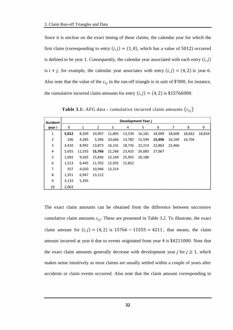
Since it is unclear on the exact timing of these claims, the calendar year for which the
first claim (corresponding to entry , which has a value of ) occurred
is defined to be year . Consequently, the calendar year associated with each entry
is , for example, the calendar year associates with entry is year .
Also note that the value of the in the run-off triangle is in unit of , for instance,
the cumulative incurred claim amounts for entry is .
Table 3.1: AFG data - cumulative incurred claim amounts
Accident year i
Development Year j
0 1 2 3 4 5 6 7 8 9
1 5,012 8,269 10,907 11,805 13,539 16,181 18,009 18,608 18,662 18,834
2 106 4,285 5,396 10,666 13,782 15,599 15,496 16,169 16,704
3 3,410 8,992 13,873 16,141 18,735 22,214 22,863 23,466
4 5,655 11,555 15,766 21,266 23,425 26,083 27,067
5 1,092 9,565 15,836 22,169 25,955 26,180
6 1,513 6,445 11,702 12,935 15,852
7 557 4,020 10,946 12,314
8 1,351 6,947 13,112
9 3,133 5,395
10 2,063
The exact claim amounts can be obtained from the difference between successive
cumulative claim amounts . These are presented in Table 3.2. To illustrate, the exact
claim amount for is , that means, the claim
amount incurred at year due to events originated from year is . Note that
the exact claim amounts generally decrease with development year for , which
makes sense intuitively as most claims are usually settled within a couple of years after
accidents or claim events occurred. Also note that the claim amount corresponding to
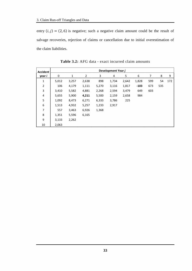
3. Claim Run-off Triangles and Data
33
entry is negative; such a negative claim amount could be the result of
salvage recoveries, rejection of claims or cancellation due to initial overestimation of
the claim liabilities.
Table 3.2: AFG data - exact incurred claim amounts
Accident year i
Development Year j
0 1 2 3 4 5 6 7 8 9
1 5,012 3,257 2,638 898 1,734 2,642 1,828 599 54 172
2 106 4,179 1,111 5,270 3,116 1,817 -103 673 535 3 3,410 5,582 4,881 2,268 2,594 3,479 649 603
4 5,655 5,900 4,211 5,500 2,159 2,658 984 5 1,092 8,473 6,271 6,333 3,786 225
6 1,513 4,932 5,257 1,233 2,917 7 557 3,463 6,926 1,368
8 1,351 5,596 6,165 9 3,133 2,262
10 2,063

34
CHAPTER 4
BBaayyeessiiaann MMooddeellll iinngg ooff tthhee AAFFGG DDaattaa
4.1 Reserving methods
As discussed in Chapter 1, deterministic approaches to reserving include the traditional
chain-ladder (CL) method and the Bornhuetter-Ferguson method. However, these
approaches only provide point estimates of the required reserve. Stochastic reserving
methods were considered by Scollnik (2004), England & Verrall (2002) and several
others.
The required reserve is equal to the value of outstanding claims liabilities, in which the
liabilities may or may not discounted to present value. In the thesis, the outstanding
claims liabilities are not discounted to present value, this is to facilitate comparison
between different reserving methods. Note that the actual reserve held in practice might
not be the same as the required reserve; it is conservative to ensure that the actual
reserve is at least as great as the required reserve. For convenience the term „reserve‟
will be used to mean the required reserve instead of actual reserve in this thesis.
More precisely, in a claim run-off triangle showing exact claim amounts (such as the
one in Table 3.2), the reserve is equal to the sum of the claim liabilities associated with
the lower triangle, which need to be estimated. Equivalently, for a cumulative claim
run-off triangle (such as in Table 3.1), the reserve has the following formula:
where is the number of rows or columns (assuming a square run-off triangle).

4. Bayesian Modelling of the AFG Data
35
It is important to note that the accident year starts from while the development year
starts from .
This thesis develops Bayesian models based on classical reserving models first
proposed by Hertig (1985) and later extended by de Jong (2004). These Bayesian
models, together with their classical counterparts, are discussed in the following section.
4.2 Bayesian models
Consider a run-off triangle with entries which represents the cumulative claim
liabilities for accident years and development years . Define the development factors
for as the continuous growth rates in cumulative claim liabilities of accident
years in development year , and formulate this quantity as the log-link ratio. Also
define as the natural logarithm of the initial claim liabilities of accident year . Thus:
The variable denotes number of years for which data are available; note that the claim
run-off triangle considered in the thesis (AFG data) has equal numbers of rows and
columns.
The development factors are calculated and displayed in Table 4.1. Note that one of
the development factors is negative, which corresponds to the negative
incremental claim. Besides, the for which appears to be exceptionally large
compared to the rest; this is due to the difference in the definition of the development

4. Bayesian Modelling of the AFG Data
36
factors, for which are not the growth rates of the cumulative claims. Also note that
the development factors tend to decrease across development years.
Table 4.1: AFG data - development factors
Accident year i
Development Year j
0 1 2 3 4 5 6 7 8 9
1 8.520 0.501 0.277 0.079 0.137 0.178 0.107 0.033 0.003 0.009
2 4.663 3.699 0.231 0.681 0.256 0.124 -0.007 0.043 0.033
3 8.134 0.970 0.434 0.151 0.149 0.170 0.029 0.026
4 8.640 0.715 0.311 0.299 0.097 0.107 0.037
5 6.996 2.170 0.504 0.336 0.158 0.009
6 7.322 1.449 0.596 0.100 0.203
7 6.323 1.976 1.002 0.118
8 7.209 1.637 0.635
9 8.050 0.543
10 7.632
Hertig (1985) made an assumption that the development factors are uncorrelated and
can be written in the following form:
(1)
Hence, each has a normal distribution with mean and variance ; that is,
In this model (which will hereafter be called Hertig‟s model), is set to to avoid
over-parameterisation. Note that this model allows the incremental claim liabilities to
take negative values, since it is possible for the development factors to be negative.
Under the classical approach, the parameters and are assumed to be unknown
constants that need to be estimated, either by maximum likelihood estimation or the

4. Bayesian Modelling of the AFG Data
37
method of moments, as, for example, in de Jong (2004). In contrast, the Bayesian
approach treats the parameters and as random variables, with a joint prior
distribution. Often these parameters are taken as a priori independent, uninformative
and improper, as follows:
As mentioned before, care must be taken when using improper priors since this might
lead to posterior distributions being improper, giving nonsensical inference. Note that
actuaries typically have some prior knowledge regarding the parameters, which may be
available through past experience, or simply based on their actuarial judgement; the
prior distributions can then be modified accordingly.
Hertig‟s model assumes that the growth rates across accident years have the same
distribution on each development year . However, de Jong found that the development
factors are correlated and suggested adding correlation terms to Hertig‟s model. The
following are three different modifications to Hertig‟s model (1) suggested by de Jong.
i. (2)
This defines the development correlation model. Here, correlation of the
development factors across development years is captured by the
parameter . This model asserts that the magnitude of each directly
influences the development factors for the next year, .

4. Bayesian Modelling of the AFG Data
38
ii.
Under this accident correlation model, correlation of the development factors
across accident years is modelled by the parameters and .
iii.
This calendar correlation model introduces the parameters and to
model the correlation of across calendar years.
Bayesian implementation of Hertig‟s model and the development correlation model (2)
will be discussed in detail in Chapter 5. Note that, for simplicity, the term “Hertig‟s
model” will refer to the Bayesian implementation of Hertig‟s model rather than its
classical counterpart.

39
CHAPTER 5
AAnnaallyyssiiss aanndd RReessuull ttss
5.1 Hertig‟s model
Hertig‟s model, introduced in Section 4.2, will be used in this chapter to model the AFG
data. Ideally, the prior distributions of this model‟s parameters are uninformative and
improper, as follows:
However, as the modelling will be done in WinBUGS, which does not allow priors to be
improper, the following vague prior distributions are chosen in an attempt to give the
best representation of the uninformative and improper priors:
Note that choosing a prior distribution which is more diffuse for and , such as
, leads to an error message in WinBUGS. This is because the
software cannot accept priors that are too diffuse. Since there are parameters to be
estimated from only data points, the resulting posterior distributions end up being
improper. (If there were many more data points to estimate the same number of
parameters, the posterior might be proper.)

5. Analysis and Results
40
The WinBUGS code for this model is presented in Appendix C-3. With the starting
points chosen to be , and , simulated values of each
parameter were created (in 6 seconds, with the same processor described above) via the
Gibbs sampler. By burning-in the first simulated values, estimates of the posterior
means were obtained from the remaining simulations; the WinBUGS output is
displayed in Table 5.1. Classical estimates by de Jong are included for comparison.
Note that in Table 5.1, each h[j ] corresponds to parameter , while each mu[j]
corresponds to parameter and sigma2 corresponds to parameter .
Table 5.1: Posterior estimates of , and (Hertig‟s model)
node mean sd MC error 2.5% median 97.5% de Jong’s
h[2] 0.9654 0.3503 0.008836 0.4693 0.9088 1.793 0.8571 h[3] 0.2448 0.09868 0.002577 0.1122 0.2254 0.4892 0.2143 h[4] 0.2142 0.09374 0.002222 0.09399 0.195 0.4497 0.1786 h[5] 0.05783 0.02786 6.26E-4 0.02417 0.05152 0.1309 0.0446 h[6] 0.07323 0.04005 9.275E-4 0.02874 0.06386 0.1738 0.0536 h[7] 0.05735 0.04021 8.36E-4 0.01953 0.04666 0.1623 0.0357 h[8] 0.01322 0.01739 5.151E-4 0.003171 0.008864 0.04989 0.0089 h[9] 0.09772 0.3435 0.01146 0.006977 0.02854 0.6174 0.0089 h[10] 0.8656 3.246 0.1542 3.468E-10 0.001739 9.444 0.00 mu[1] 7.346 0.4009 0.003863 6.549 7.345 8.147 7.35
mu[2] 1.518 0.3938 0.004067 0.7263 1.518 2.311 1.52 mu[3] 0.4981 0.1079 0.001066 0.2839 0.4984 0.7141 0.50 mu[4] 0.2515 0.1006 0.00104 0.04582 0.2527 0.4482 0.25 mu[5] 0.1666 0.0297 3.031E-4 0.1069 0.1667 0.226 0.17 mu[6] 0.1182 0.04235 4.402E-4 0.03564 0.1178 0.2026 0.12 mu[7] 0.0409 0.04056 4.143E-4 -0.03797 0.04104 0.118 0.04 mu[8] 0.03362 0.01372 1.166E-4 0.01118 0.03389 0.05449 0.03 mu[9] 0.01951 0.2885 0.001898 -0.1811 0.01824 0.24 0.02 mu[10] -0.01621 3.873 0.03726 -3.992 0.009174 4.147 0.01
sigma2 1.612 0.8962 0.03325 0.626 1.387 3.965 1.2544
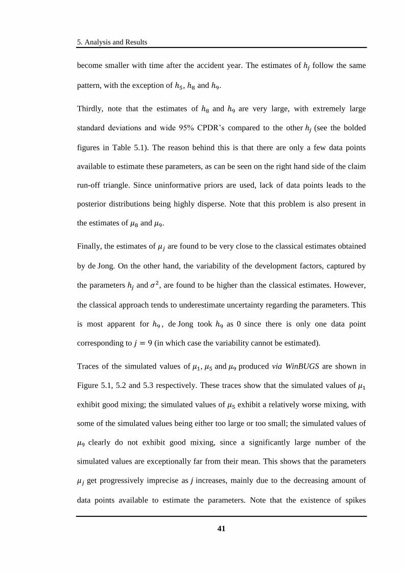
There are a few points that should be noted. First, the posterior estimate of is
exceptionally large ( , bolded above) compared to other . This is purely
due to the fact that the development factors for are fundamentally different
in definition to the other development factors. Secondly, is estimated to be smaller as
development year gets larger; this makes sense intuitively, because total claims tend to
5. Analysis and Results
41
become smaller with time after the accident year. The estimates of follow the same
pattern, with the exception of , and .
Thirdly, note that the estimates of and are very large, with extremely large
standard deviations and wide 95% CPDR‟s compared to the other (see the bolded
figures in Table 5.1). The reason behind this is that there are only a few data points
available to estimate these parameters, as can be seen on the right hand side of the claim
run-off triangle. Since uninformative priors are used, lack of data points leads to the
posterior distributions being highly disperse. Note that this problem is also present in
the estimates of and .
Finally, the estimates of are found to be very close to the classical estimates obtained
by de Jong. On the other hand, the variability of the development factors, captured by
the parameters and , are found to be higher than the classical estimates. However,
the classical approach tends to underestimate uncertainty regarding the parameters. This
is most apparent for , de Jong took as since there is only one data point
corresponding to (in which case the variability cannot be estimated).
Traces of the simulated values of , and produced via WinBUGS are shown in
Figure 5.1, 5.2 and 5.3 respectively. These traces show that the simulated values of
exhibit good mixing; the simulated values of exhibit a relatively worse mixing, with
some of the simulated values being either too large or too small; the simulated values of
clearly do not exhibit good mixing, since a significantly large number of the
simulated values are exceptionally far from their mean. This shows that the parameters
get progressively imprecise as increases, mainly due to the decreasing amount of
data points available to estimate the parameters. Note that the existence of spikes

5. Analysis and Results
42
(extremely large values) in Figure 5.3 is the primary reason for the high standard
deviation of the estimate (see Table 5.1). The traces of the simulated are similar
and give the same inference for . The traces of simulated , and are shown in
Appendix D-2 for completeness.
Figure 5.1: Trace of simulated
Figure 5.2: Trace of simulated
Figure 5.3: Trace of simulated
mu[2]
iteration
1 5000 10000
-2.0
0.0
2.0
4.0
mu[6]
iteration
1 5000 10000
-0.5
0.0
0.5
1.0
mu[10]
iteration
1 5000 10000
-150.0
-100.0
-50.0
0.0
50.0
100.0

5. Analysis and Results
43
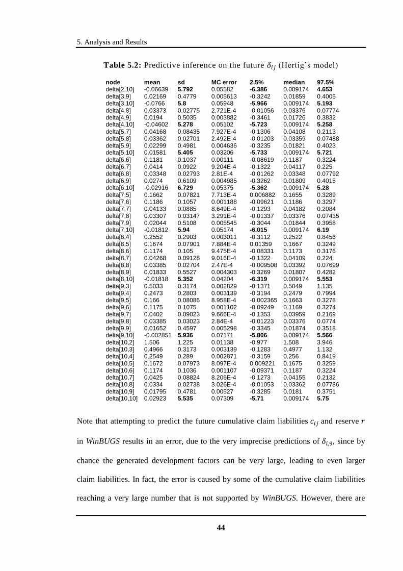
Predictive inference on the future development factors can be obtained by generating
random observations of the future development factors directly. In WinBUGS, this is
easily done by specifying the distribution of the future development factors, which is no
different from the distribution of the current development factors, as defined in
Section 4.2. In addition, the future cumulative claim liabilities and the reserve are
readily obtained since they can be expressed as explicit functions of the future
development factors. The predictive inference is presented in Table 5.2 in the same
format as Table 5.1; again, note that each delta[ i, j ] corresponds to the development
factor .
Most of the predicted development factors are reasonable predictions of the future,
except for development years and , where the high variability in predictions is
caused by the imprecise posterior estimates of the underlying parameters. For instance,
the prediction of (delta[10,10] in Table 5.2) is accompanied by an extremely large
standard deviation and a very wide 95% prediction interval .
These large standard deviations and prediction intervals are bolded in Table 5.2; they
correspond to the estimates where . These predictions do not provide any real
information regarding the future claim amounts, because a single data point is
insufficient to project future claim payments. For example, the 95% prediction interval
for suggests that the cumulative claim liabilities for next year will be between
and of the current cumulative claim.
5. Analysis and Results
44
Table 5.2: Predictive inference on the future (Hertig‟s model)
node mean sd MC error 2.5% median 97.5% delta[2,10] -0.06639 5.792 0.05582 -6.386 0.009174 4.653
delta[3,9] 0.02169 0.4779 0.005613 -0.3242 0.01859 0.4005 delta[3,10] -0.0766 5.8 0.05948 -5.966 0.009174 5.193
delta[4,8] 0.03373 0.02775 2.721E-4 -0.01056 0.03376 0.07774 delta[4,9] 0.0194 0.5035 0.003882 -0.3461 0.01726 0.3832 delta[4,10] -0.04602 5.278 0.05102 -5.723 0.009174 5.258
delta[5,7] 0.04168 0.08435 7.927E-4 -0.1306 0.04108 0.2113 delta[5,8] 0.03362 0.02701 2.492E-4 -0.01203 0.03359 0.07488 delta[5,9] 0.02299 0.4981 0.004636 -0.3235 0.01821 0.4023 delta[5,10] 0.01581 5.405 0.03206 -5.733 0.009174 5.721
delta[6,6] 0.1181 0.1037 0.00111 -0.08619 0.1187 0.3224 delta[6,7] 0.0414 0.0922 9.204E-4 -0.1322 0.04117 0.225 delta[6,8] 0.03348 0.02793 2.81E-4 -0.01262 0.03348 0.07792 delta[6,9] 0.0274 0.6109 0.004985 -0.3262 0.01809 0.4015 delta[6,10] -0.02916 6.729 0.05375 -5.362 0.009174 5.28
delta[7,5] 0.1662 0.07821 7.713E-4 0.006882 0.1655 0.3289 delta[7,6] 0.1186 0.1057 0.001188 -0.09621 0.1186 0.3297 delta[7,7] 0.04133 0.0885 8.649E-4 -0.1293 0.04182 0.2084 delta[7,8] 0.03307 0.03147 3.291E-4 -0.01337 0.03376 0.07435 delta[7,9] 0.02044 0.5108 0.005545 -0.3044 0.01844 0.3958 delta[7,10] -0.01812 5.94 0.05174 -6.015 0.009174 6.19
delta[8,4] 0.2552 0.2903 0.003011 -0.3112 0.2522 0.8456 delta[8,5] 0.1674 0.07901 7.884E-4 0.01359 0.1667 0.3249 delta[8,6] 0.1174 0.105 9.475E-4 -0.08331 0.1173 0.3176 delta[8,7] 0.04268 0.09128 9.016E-4 -0.1322 0.04109 0.224 delta[8,8] 0.03385 0.02704 2.47E-4 -0.009508 0.03392 0.07699 delta[8,9] 0.01833 0.5527 0.004303 -0.3269 0.01807 0.4282 delta[8,10] -0.01818 5.352 0.04204 -6.319 0.009174 5.553
delta[9,3] 0.5033 0.3174 0.002829 -0.1371 0.5049 1.135 delta[9,4] 0.2473 0.2803 0.003139 -0.3194 0.2479 0.7994 delta[9,5] 0.166 0.08086 8.958E-4 -0.002365 0.1663 0.3278 delta[9,6] 0.1175 0.1075 0.001102 -0.09249 0.1169 0.3274 delta[9,7] 0.0402 0.09023 9.666E-4 -0.1353 0.03959 0.2169 delta[9,8] 0.03385 0.03023 2.84E-4 -0.01223 0.03376 0.0774 delta[9,9] 0.01652 0.4597 0.005298 -0.3345 0.01874 0.3518 delta[9,10] -0.002851 5.936 0.07171 -5.806 0.009174 5.566
delta[10,2] 1.506 1.225 0.01138 -0.977 1.508 3.946 delta[10,3] 0.4966 0.3173 0.003139 -0.1283 0.4977 1.132 delta[10,4] 0.2549 0.289 0.002871 -0.3159 0.256 0.8419 delta[10,5] 0.1672 0.07973 8.097E-4 0.009221 0.1675 0.3259 delta[10,6] 0.1174 0.1036 0.001107 -0.09371 0.1187 0.3224 delta[10,7] 0.0425 0.08824 8.206E-4 -0.1273 0.04155 0.2132 delta[10,8] 0.0334 0.02738 3.026E-4 -0.01053 0.03362 0.07786 delta[10,9] 0.01795 0.4781 0.00527 -0.3285 0.0181 0.3751 delta[10,10] 0.02923 5.535 0.07309 -5.71 0.009174 5.75
Note that attempting to predict the future cumulative claim liabilities and reserve
in WinBUGS results in an error, due to the very imprecise predictions of , since by
chance the generated development factors can be very large, leading to even larger
claim liabilities. In fact, the error is caused by some of the cumulative claim liabilities
reaching a very large number that is not supported by WinBUGS. However, there are

5. Analysis and Results
45
ways to achieve the predictive inference on the cumulative claim liabilities and the
reserve. One method is to reduce the number of effective simulations . The other is to
explicitly set an upper bound for the predicted development factors. The predictive
inference obtained via the first method with is shown in Appendix D-3 for
completeness. A snapshot of the predictive inference is shown in Table 5.3. This
inference is not entirely useful, since the predicted reserve is unreasonably large.
Table 5.3: Predictive inference on reserve (Hertig‟s model)
node mean sd MC error 2.5% median 97.5% reserve 1.086E+33 4.406E+34 1.067E+33 -75100.0 86260.0 5.208E+11
5.2 A modified Hertig‟s model
As can be seen in the previous section, using a single data point for estimation leads to
extremely large standard deviations and hence imprecise estimates. This calls for a
modification to Hertig‟s model that rectifies this problem. Since the parameters and
decrease with development years , one possible approach is to model the structure of
and directly. Assuming and decrease exponentially for , the following
parameterisation was used as a „fix‟ to Hertig‟s model:

5. Analysis and Results
46
The vague prior distributions associated with this modification are as follows:
where forces the simulated values of to be positive (this notation is consistent
with WinBUGS syntax).
These priors are not really uninformative; for instance, the parameters , and are
deliberately restricted to be positive since it is assumed that the mean of the
development factors are positive (a development factor can still be negative under this
model). This assumption is supported by the MCMC estimates in Table 5.1.
This modification reduces the number of parameters that need to be estimated from
to and assumes that and decrease exponentially with a constant rate. (This
assumption could be relaxed by allowing and to decrease with varying rates, but
this would increase the required number of parameters.)
As in Section 5.1, Gibbs sampling was used to simulate values of each
parameter. The starting points were chosen to be , , ,
and . The WinBUGS code for this model is presented in Appendix C-4. Again, a
burn-in of was chosen so that a final sample of simulated values
were used in producing the posterior mean estimates, as shown by the WinBUGS
5. Analysis and Results
47
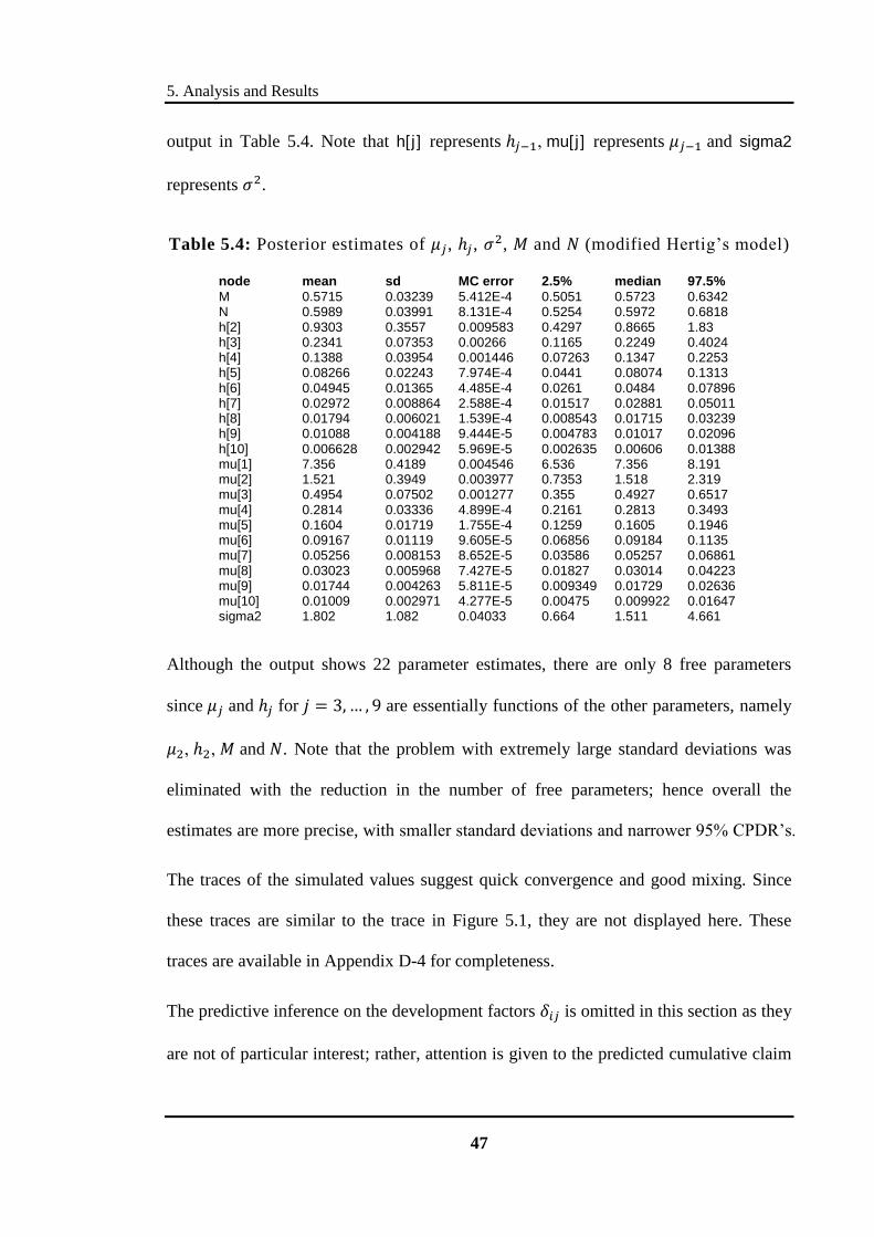
output in Table 5.4. Note that h[j ] represents mu[j] represents and sigma2
represents .
Table 5.4: Posterior estimates of , , , and (modified Hertig‟s model)
node mean sd MC error 2.5% median 97.5%
M 0.5715 0.03239 5.412E-4 0.5051 0.5723 0.6342 N 0.5989 0.03991 8.131E-4 0.5254 0.5972 0.6818 h[2] 0.9303 0.3557 0.009583 0.4297 0.8665 1.83 h[3] 0.2341 0.07353 0.00266 0.1165 0.2249 0.4024 h[4] 0.1388 0.03954 0.001446 0.07263 0.1347 0.2253 h[5] 0.08266 0.02243 7.974E-4 0.0441 0.08074 0.1313 h[6] 0.04945 0.01365 4.485E-4 0.0261 0.0484 0.07896 h[7] 0.02972 0.008864 2.588E-4 0.01517 0.02881 0.05011 h[8] 0.01794 0.006021 1.539E-4 0.008543 0.01715 0.03239 h[9] 0.01088 0.004188 9.444E-5 0.004783 0.01017 0.02096 h[10] 0.006628 0.002942 5.969E-5 0.002635 0.00606 0.01388 mu[1] 7.356 0.4189 0.004546 6.536 7.356 8.191 mu[2] 1.521 0.3949 0.003977 0.7353 1.518 2.319 mu[3] 0.4954 0.07502 0.001277 0.355 0.4927 0.6517 mu[4] 0.2814 0.03336 4.899E-4 0.2161 0.2813 0.3493 mu[5] 0.1604 0.01719 1.755E-4 0.1259 0.1605 0.1946 mu[6] 0.09167 0.01119 9.605E-5 0.06856 0.09184 0.1135 mu[7] 0.05256 0.008153 8.652E-5 0.03586 0.05257 0.06861 mu[8] 0.03023 0.005968 7.427E-5 0.01827 0.03014 0.04223 mu[9] 0.01744 0.004263 5.811E-5 0.009349 0.01729 0.02636 mu[10] 0.01009 0.002971 4.277E-5 0.00475 0.009922 0.01647 sigma2 1.802 1.082 0.04033 0.664 1.511 4.661
Although the output shows 22 parameter estimates, there are only 8 free parameters
since and for are essentially functions of the other parameters, namely
and . Note that the problem with extremely large standard deviations was
eliminated with the reduction in the number of free parameters; hence overall the
estimates are more precise, with smaller standard deviations and narrower 95% CPDR‟s.
The traces of the simulated values suggest quick convergence and good mixing. Since
these traces are similar to the trace in Figure 5.1, they are not displayed here. These
traces are available in Appendix D-4 for completeness.
The predictive inference on the development factors is omitted in this section as they
are not of particular interest; rather, attention is given to the predicted cumulative claim

5. Analysis and Results
48
liabilities and the reserve . Unlike in the preceding section, obtaining the predictive
inference with WinBUGS did not produce any error messages under modified Hertig‟s
model. The predictive inference is shown in Table 5.5, where c.pred[i, j ] represents
.
Table 5.5: Predictive inference on future and (modified Hertig‟s model)
node mean sd MC error 2.5% median 97.5%
c.pred[2,10] 16880.0 156.3 1.714 16560.0 16870.0 17190.0 c.pred[3,9] 23880.0 353.2 3.316 23180.0 23880.0 24590.0 c.pred[3,10] 24130.0 439.0 4.899 23260.0 24120.0 25030.0 c.pred[4,8] 27910.0 655.7 6.95 26640.0 27900.0 29270.0 c.pred[4,9] 28410.0 813.4 8.835 26860.0 28380.0 30080.0 c.pred[4,10] 28700.0 894.5 9.416 26990.0 28670.0 30520.0 c.pred[5,7] 27620.0 1043.0 11.59 25630.0 27600.0 29750.0 c.pred[5,8] 28470.0 1292.0 13.94 2.6E+4 28430.0 31170.0 c.pred[5,9] 28970.0 1414.0 15.03 26280.0 28930.0 31950.0 c.pred[5,10] 29270.0 1488.0 15.95 26450.0 29240.0 32410.0 c.pred[6,6] 17400.0 1082.0 12.43 15350.0 17390.0 19600.0 c.pred[6,7] 18360.0 1363.0 14.68 15820.0 18340.0 21140.0 c.pred[6,8] 18940.0 1497.0 16.04 16130.0 18890.0 2.2E+4 c.pred[6,9] 19280.0 1576.0 17.08 16310.0 19230.0 22480.0 c.pred[6,10] 19480.0 1620.0 17.67 16460.0 19430.0 22800.0 c.pred[7,5] 14510.0 1495.0 14.65 11750.0 14440.0 17650.0 c.pred[7,6] 15930.0 1933.0 16.63 12430.0 15800.0 20100.0 c.pred[7,7] 16800.0 2148.0 19.32 12930.0 16680.0 21380.0 c.pred[7,8] 17330.0 2278.0 20.47 13220.0 17200.0 22210.0 c.pred[7,9] 17640.0 2349.0 21.58 13430.0 17500.0 22610.0 c.pred[7,10] 17820.0 2394.0 22.12 13520.0 17670.0 22850.0 c.pred[8,4] 17660.0 3083.0 29.1 12320.0 17440.0 24550.0 c.pred[8,5] 20870.0 4328.0 44.65 13630.0 20410.0 30770.0 c.pred[8,6] 22940.0 5010.0 51.31 14710.0 22360.0 34300.0 c.pred[8,7] 24190.0 5397.0 55.24 15300.0 23560.0 36520.0 c.pred[8,8] 24930.0 5605.0 57.34 15750.0 24330.0 37490.0 c.pred[8,9] 25380.0 5731.0 57.99 15980.0 24760.0 38320.0 c.pred[8,10] 25640.0 5809.0 58.94 16100.0 25010.0 38800.0 c.pred[9,3] 9257.0 2985.0 29.61 4822.0 8820.0 16360.0 c.pred[9,4] 12460.0 4767.0 51.21 5722.0 11650.0 23820.0 c.pred[9,5] 14740.0 5955.0 62.2 6419.0 13640.0 29150.0 c.pred[9,6] 16170.0 6634.0 69.65 6983.0 14940.0 32230.0 c.pred[9,7] 17070.0 7058.0 72.4 7357.0 15750.0 34270.0 c.pred[9,8] 17610.0 7296.0 74.11 7542.0 16230.0 35350.0 c.pred[9,9] 17920.0 7428.0 74.93 7676.0 16500.0 36020.0 c.pred[9,10] 18110.0 7505.0 75.27 7761.0 16680.0 36380.0 c.pred[10,2] 22130.0 88610.0 1015.0 782.1 9544.0 109500.0 c.pred[10,3] 38080.0 160200.0 1827.0 1212.0 15580.0 190200.0 c.pred[10,4] 51080.0 205700.0 2417.0 1554.0 20680.0 2.6E+5 c.pred[10,5] 60160.0 234100.0 2763.0 1813.0 24260.0 313600.0 c.pred[10,6] 66330.0 2.59E+5 3071.0 2014.0 26690.0 347300.0 c.pred[10,7] 70180.0 280900.0 3318.0 2104.0 28120.0 368700.0 c.pred[10,8] 72380.0 289400.0 3424.0 2167.0 29050.0 377700.0 c.pred[10,9] 73690.0 295300.0 3485.0 2215.0 29620.0 383600.0 c.pred[10,10] 74390.0 296400.0 3498.0 2219.0 29850.0 386700.0 reserve 112300.0 296700.0 3498.0 30740.0 69700.0 424500.0
5. Analysis and Results
49
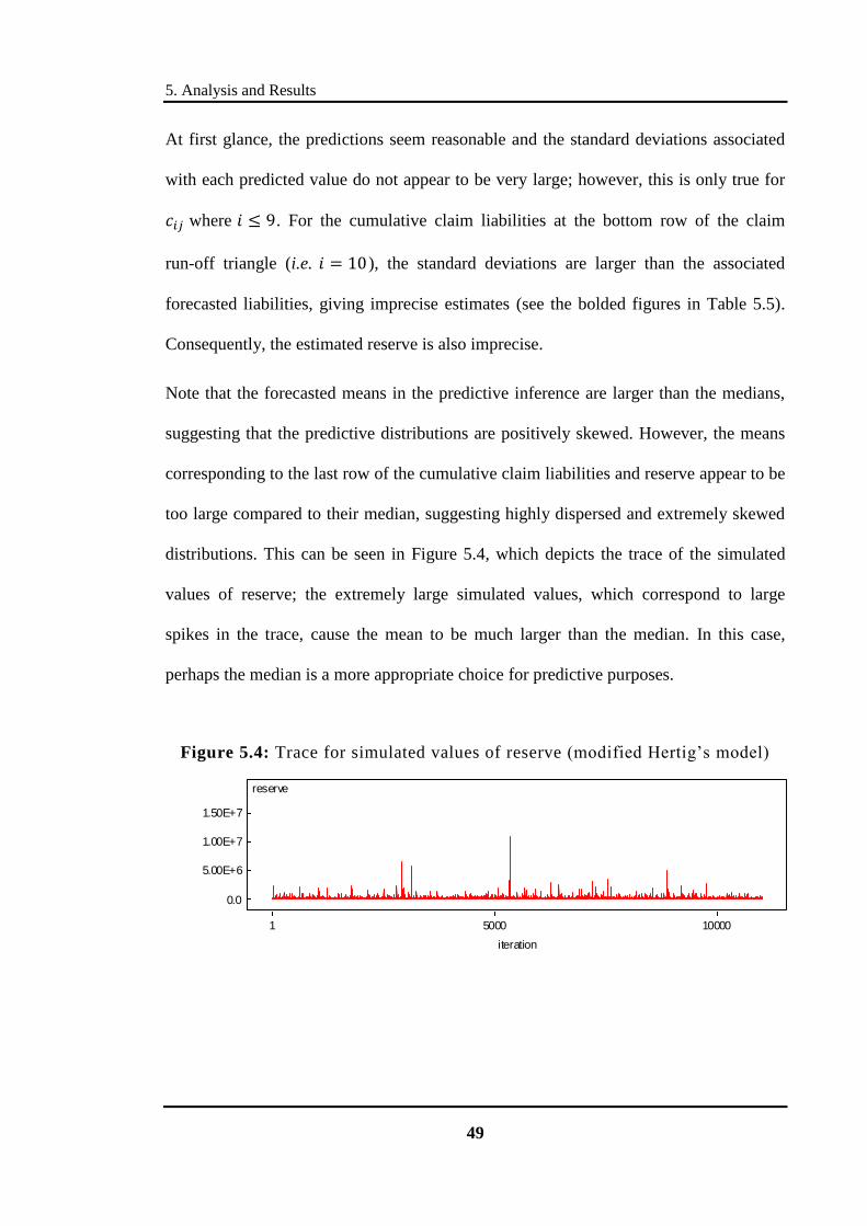
At first glance, the predictions seem reasonable and the standard deviations associated
with each predicted value do not appear to be very large; however, this is only true for
where . For the cumulative claim liabilities at the bottom row of the claim
run-off triangle (i.e. ), the standard deviations are larger than the associated
forecasted liabilities, giving imprecise estimates (see the bolded figures in Table 5.5).
Consequently, the estimated reserve is also imprecise.
Note that the forecasted means in the predictive inference are larger than the medians,
suggesting that the predictive distributions are positively skewed. However, the means
corresponding to the last row of the cumulative claim liabilities and reserve appear to be
too large compared to their median, suggesting highly dispersed and extremely skewed
distributions. This can be seen in Figure 5.4, which depicts the trace of the simulated
values of reserve; the extremely large simulated values, which correspond to large
spikes in the trace, cause the mean to be much larger than the median. In this case,
perhaps the median is a more appropriate choice for predictive purposes.
Figure 5.4: Trace for simulated values of reserve (modified Hertig‟s model)
reserve
iteration
1 5000 10000
0.0
5.00E+6
1.00E+7
1.50E+7

5. Analysis and Results
50
The large standard deviations corresponding to the bottom row of the cumulative claim
liabilities is most likely to be caused by the imprecise forecast of (c.pred[10,2] in
Table 5.5) initially, and this causes the following cumulative claim liabilities to be
highly variable, ultimately the estimated reserve as well. It is possible that the model is
lacking something in explaining the development factors when , such as the
correlation between the development factors. In fact, ignoring the correlation between
and can lead to sizable forecast errors (de Jong, 2004). Correlation between the
development factors will be implemented in the following section.
5.3 Development correlation model
In this section, the development correlation model (see Equation 2 in Section 4.2) is
further discussed. Note that this model assumes first order correlation between each
consecutive pair of the development factors, in the sense that each is correlated with
for ; this is captured by the correlation parameters .
The same modification from Section 5.2 will be applied to this model (i.e. applying
structural constraints to and for ), to avoid large standard deviations that
accompany the MCMC estimates (for and when ). The introduction of the
correlation terms will increase the number of free parameters by , which is undesirable
given the number of data points. For purposes of parsimony, only the correlation
between and will be considered, meaning that only one extra parameter will
be added to the model. This is consistent with de Jong‟s assumption that only the
correlation between development years and is significant.

5. Analysis and Results
51
The resulting development correlation model may be summarised as follows:
The prior distributions in this model are exactly the same as those in Section 5.2, with
the addition of the prior distribution for , as follows:
Note that there are only 9 free parameters in this model. The WinBUGS code of this
model is in Appendix C-5. Again, Gibbs sampling was used to simulate
values of each parameter, the starting points were chosen to be
and and values were burnt-in.
The posterior estimates are shown below in Table 5.6. Note that the estimate
of is also presented in Table 5.6. As above, h[j ]
represents mu[j] represents and sigma2 represents . Also, theta and rho
represent and , respectively.
The results in Table 5.6 are similar to those in Table 5.4, but with two extra rows. The
estimated and show that the development factors between development years and
are negatively and significantly correlated, also note that none of the standard
deviations in Table 5.6 seem to be unduly large.

5. Analysis and Results
52
Table 5.6: Posterior estimates (development correlation model)
node mean sd MC error 2.5% median 97.5%
M 0.5711 0.03266 5.617E-4 0.5053 0.5718 0.6351 N 0.5986 0.04001 9.132E-4 0.5266 0.5965 0.6829 h[2] 0.2221 0.08752 0.004816 0.09138 0.21 0.4286 h[3] 0.2238 0.075 0.003573 0.1025 0.2147 0.3959 h[4] 0.1325 0.04036 0.002011 0.06373 0.1292 0.2226 h[5] 0.07883 0.02281 0.001146 0.03887 0.07742 0.128 h[6] 0.04711 0.01375 6.633E-4 0.02317 0.04623 0.07715 h[7] 0.02828 0.008831 3.906E-4 0.01361 0.02742 0.04804 h[8] 0.01706 0.005944 2.344E-4 0.007901 0.01626 0.03096 h[9] 0.01034 0.00411 1.435E-4 0.00446 0.009662 0.02039 h[10] 0.006295 0.002878 8.963E-5 0.002477 0.005728 0.01349 mu[1] 7.38 0.4209 0.01947 6.547 7.382 8.21 mu[2] 1.467 0.3476 0.01601 0.7851 1.463 2.147 mu[3] 0.4967 0.07618 0.001229 0.3518 0.4949 0.6543 mu[4] 0.2819 0.03399 4.692E-4 0.2153 0.2815 0.35 mu[5] 0.1606 0.01754 1.775E-4 0.1259 0.1607 0.1951 mu[6] 0.09172 0.01138 1.087E-4 0.06868 0.09181 0.1135 mu[7] 0.05256 0.008263 9.531E-5 0.03594 0.05265 0.06871 mu[8] 0.03021 0.006035 7.938E-5 0.01847 0.03017 0.0425 mu[9] 0.01742 0.004305 6.115E-5 0.009435 0.01728 0.02645 mu[10] 0.01008 0.002996 4.467E-5 0.004837 0.009887 0.01657 rho -0.9576 0.03492 0.001646 -0.9936 -0.9666 -0.8645
sigma2 2.082 1.597 0.09705 0.7158 1.653 6.188 theta -4.141 1.836 0.1221 -8.785 -3.769 -1.72
The traces of the simulated values illustrate that the simulations converge very quickly
and produce reasonably good mixing. Figures 5.5, 5.6 and 5.7 shows the traces of
simulated and , while the rest of the traces are placed in Appendix D-5.
However, most of the simulated values appear to have higher autocorrelation, causing
the standard deviations to underestimate the true variability of the parameters; hence,
the MC errors are more suitable in measuring the variability. Note that the introduction
of to the model causes the simulated values of and to be negatively correlated,
which can be seen from the traces in Figure 5.5 and 5.6. In fact, by plotting the
simulated values of against those of , the negative relationship is obvious (the plot
is shown in Figure 8.6 in Appendix D-6).

5. Analysis and Results
53
Figure 5.5: Trace of
Figure 5.6: Trace of
Figure 5.7: Trace of
mu[1]
iteration
1 5000 10000
5.0
6.0
7.0
8.0
9.0
10.0
mu[2]
iteration
1 5000 10000
0.0
1.0
2.0
3.0
4.0
theta
iteration
1 5000 10000
-15.0
-10.0
-5.0
0.0
5.0

5. Analysis and Results
54
Predictive inference on the individual future cumulative claim liabilities and the total
reserve are presented in Table 5.7.
Table 5.7: Predictive inference on and (development correlation model)
node mean sd MC error 2.5% median 97.5%
c.pred[2,10] 16880.0 159.1 1.748 16560.0 16870.0 17200.0 c.pred[3,9] 23880.0 355.1 3.685 23180.0 23880.0 24590.0 c.pred[3,10] 24130.0 439.8 4.638 23250.0 24120.0 25020.0 c.pred[4,8] 27920.0 655.2 7.266 26650.0 27900.0 29220.0 c.pred[4,9] 28410.0 815.3 8.964 26840.0 28390.0 30060.0 c.pred[4,10] 28700.0 896.5 10.07 26920.0 28680.0 30530.0 c.pred[5,7] 27610.0 1044.0 9.948 25590.0 27590.0 29740.0 c.pred[5,8] 28470.0 1307.0 11.45 25960.0 28450.0 31190.0 c.pred[5,9] 28980.0 1424.0 12.59 26240.0 28950.0 31900.0 c.pred[5,10] 29270.0 1495.0 13.34 26380.0 29240.0 32360.0 c.pred[6,6] 17390.0 1080.0 10.48 15340.0 17350.0 19590.0 c.pred[6,7] 18330.0 1348.0 12.66 15840.0 18280.0 21100.0 c.pred[6,8] 18910.0 1494.0 13.91 16170.0 18850.0 22060.0 c.pred[6,9] 19240.0 1571.0 14.24 16340.0 19180.0 22590.0 c.pred[6,10] 19440.0 1616.0 14.91 16470.0 19360.0 22870.0 c.pred[7,5] 14530.0 1508.0 13.32 11810.0 14440.0 17700.0 c.pred[7,6] 15940.0 1953.0 18.26 12490.0 15830.0 20140.0 c.pred[7,7] 16820.0 2192.0 19.77 12970.0 16660.0 21490.0 c.pred[7,8] 17350.0 2326.0 20.86 13200.0 17180.0 22350.0 c.pred[7,9] 17660.0 2402.0 21.42 13420.0 17500.0 22840.0 c.pred[7,10] 17840.0 2450.0 21.77 13490.0 17680.0 23080.0 c.pred[8,4] 17600.0 3120.0 32.63 12200.0 17330.0 24560.0 c.pred[8,5] 20790.0 4332.0 44.85 13490.0 20320.0 30540.0 c.pred[8,6] 22820.0 4999.0 49.97 14510.0 22300.0 34030.0 c.pred[8,7] 24050.0 5385.0 53.24 15130.0 23480.0 36200.0 c.pred[8,8] 24810.0 5618.0 55.25 15530.0 24210.0 37260.0 c.pred[8,9] 25260.0 5754.0 55.92 15770.0 24640.0 37970.0 c.pred[8,10] 25520.0 5829.0 56.5 15940.0 24890.0 38490.0 c.pred[9,3] 9248.0 2873.0 27.15 4924.0 8836.0 15990.0 c.pred[9,4] 12460.0 4627.0 46.75 5759.0 11720.0 23380.0 c.pred[9,5] 14740.0 5793.0 62.45 6544.0 13800.0 28850.0 c.pred[9,6] 16190.0 6488.0 71.32 7012.0 15140.0 31890.0 c.pred[9,7] 17080.0 6873.0 74.87 7348.0 15970.0 33770.0 c.pred[9,8] 17610.0 7097.0 76.51 7549.0 16440.0 34820.0 c.pred[9,9] 17910.0 7224.0 77.09 7693.0 16710.0 35510.0 c.pred[9,10] 18100.0 7297.0 77.59 7774.0 16870.0 35860.0 c.pred[10,2] 7670.0 2460.0 28.83 3913.0 7324.0 13520.0 c.pred[10,3] 13160.0 5982.0 66.39 5094.0 12050.0 27790.0 c.pred[10,4] 17750.0 8853.0 98.44 6293.0 15960.0 39680.0 c.pred[10,5] 20980.0 10800.0 121.4 7109.0 18760.0 48430.0 c.pred[10,6] 23070.0 12060.0 135.9 7753.0 20570.0 53220.0 c.pred[10,7] 24330.0 12770.0 143.6 8114.0 21670.0 55910.0 c.pred[10,8] 25080.0 13180.0 147.7 8334.0 22350.0 57720.0 c.pred[10,9] 25530.0 13420.0 150.1 8488.0 22760.0 58910.0 c.pred[10,10] 25790.0 13560.0 151.5 8575.0 22960.0 59540.0 reserve 63500.0 18640.0 205.0 35050.0 61090.0 107200.0
The predicted for are almost identical to those in the modified Hertig‟s model
(see Table 5.5); this is because the parameter estimates of in both models are very

5. Analysis and Results
55
close to one another. More importantly, the future cumulative claim liabilities and the
reserve have reasonable standard deviations which are not unduly large (see bolded
figures). Although the distributions of the predicted claim liabilities and reserve are still
positively skewed in this case, the magnitudes of the estimated means are not very large
compared to the estimated median.
As can be seen in Figure 5.8, which portrays the trace of the simulated reserve, there
appears to be no highly extreme values.
Figure 5.8: Trace of simulated reserve
Comparing Hertig‟s model modified Hertig‟s model, and the development correlation
model, it seems that the development correlation model performs best in modelling the
claim run-off triangle (AFG data). In the next chapter, these three models will be
assessed formally through hypothesis testing.
reserve
iteration
1 5000 10000
0.0
5.00E+4
1.00E+5
1.50E+5
2.00E+5
2.50E+5
56
CHAPTER 6
MMooddeell DDiiaaggnnoossttiiccss aanndd MMCCMMCC AAsssseessssmmeenntt
6.1 Hypothesis testing
In Chapter 5, some imprecise estimates obtained via MCMC methods were identified,
simply by looking at the posterior estimates and associated standard deviations. On that
basis, it was concluded that Hertig‟s model (Section 5.1) and its modification
(Section 5.2) are not suitable for reserving purposes. More formally, one could perform
hypothesis testing to assess the models. In this section, the theory of posterior predictive
p-values (ppp-values) will be used to perform hypothesis tests for assessing goodness-
of-fit. The strategy will be to generate independent replicated development factors
from their posterior predictive densities and compare them with the observed
development factors from the data. The behaviour of the replicates relative to the
original data will be used to decide whether the model is adequate.
Generally, where and are the underlying parameters that
generate the development factors. In Hertig‟s model and its modification, these
parameters are
Whereas under the development correlation model, they are:

6. Model Diagnostics and MCMC Assessment
57
The replicated development factors have the same joint distribution as that of the
. This joint distribution may be represented by writing
where,
for Hertig‟s model and its modification:
Whereas for the development correlation model:
Note that the set of all and the set of all are independent, conditional
on the set of all parameters, (e.g. under the
development correlation model). That is, .
For general goodness-of-fit testing, the null hypothesis is
tested against the alternative hypothesis ; by considering
two different test statistics as follows:

6. Model Diagnostics and MCMC Assessment
58
These test statistics measure the overall deviations of the quantities
from their respective expected values, scaled by an associated variance. Note that is
the successive difference between the development factors, while is the
corresponding successive ratio.
To test whether correlation is present in the model, first define
Thus, takes a value of when and are of different sign,
and otherwise .
Under Hertig‟s model and its modification the development factors are assumed to be
independently distributed, and hence there is no correlation between the development
factors. Thus it makes sense to test
versus
Under , it is equally likely for to be either or ; however, a simple calculation
of from the AFG data suggests otherwise for development year . The are
calculated from of the AFG data, using the classical estimates of , i.e. ,
the mean of the development factors correspond to each column. Table 6.1 shows the
values of the .

6. Model Diagnostics and MCMC Assessment
59
Table 6.1: AFG data -
Accident year i
Development Year j
0 1 2 3 4 5 6 7 8 9
1 - 1 0 0 0 1 0 1 0 0
2 - 1 1 1 0 0 1 1 0 3 - 1 0 0 0 1 1 0
4 - 1 0 1 1 0 0 5 - 1 0 0 1 0
6 - 0 1 1 1 7 - 1 0 1
8 - 1 0 9 - 1
10 -
As can be seen from the first column of Table 6.1, eight of the nine values are ,
implying that the development factors are actually correlated, i.e. when is larger than
, will be lower than , and vice versa. These observations suggest another (third)
test statistic, which can be used to formally test the significance of the correlation:
This test statistic counts the number of sign changes corresponding to and
for development year .
For the general assessment of goodness-of-fit, the ppp-value in favour of against
is defined to be:
where and ,
denotes the test statistic corresponding to
the replicates and is the set of original data.

6. Model Diagnostics and MCMC Assessment
60
The ppp-values can be estimated via MCMC methods, by the proportion of simulations
for which is smaller than :
where
is the set of all parameters at iteration and is the set of all
obtained via
the method of composition at iteration .
For the correlation test, the ppp-value in favour of against is defined as
where and
In this case, is estimated by
where
,
and
.
All hypothesis tests are conducted with 5% significance level; i.e. the null hypothesis
is rejected if the ppp-value is less than .
The implementation of the hypothesis tests for each model is discussed in the following
subsections.

6. Model Diagnostics and MCMC Assessment
61
6.1.1 Hertig‟s model
The expected value and the variance of need to be derived in order to evaluate the
test statistic . Under the null hypothesis, it can be shown that for
(where ):
For , it is not so simple to determine the expected value and the variance of
. However, with the assumption of independence between the
development factors, the expected value and the variance can be well approximated
using the delta method, as follows:
Proof of these formulae can be found in Appendix A-3. Note that the WinBUGS code
used to implement the hypothesis testing is presented with the model specification in
Appendix C-3.
For consistency, the same number of simulations and burn-in
are chosen. The ppp-values are estimated and presented in Table 6.2.
Table 6.2: Posterior predictive p-values (Hertig‟s model)
node mean sd MC error
Goodness-of-fit test: p1 0.6263 0.4838 0.005816 p2 0.3833 0.4862 0.007932 Correlation test: p3 0.0941 0.292 0.003198

6. Model Diagnostics and MCMC Assessment
62
These ppp-values imply that the overall goodness-of-fit is acceptable, where the null
hypothesis is accepted with and . For the correlation test, the
null hypothesis that the development factors are independent (not correlated) is rejected
at the 10% level but not at the 5% level. Therefore, it is concluded that Hertig‟s model
is adequate in modelling the claim run-off triangle. However, note that with scarce
amount of data, these hypothesis tests are not very strong, especially for the third
hypothesis testing, where only nine data points are used (for ).
6.1.2 Modified Hertig‟s model
Note that the modified Hertig‟s model was introduced to overcome the issue of scarce
data in estimating the parameters. This model is very similar to Hertig‟s model since
the only changes to the model is the limiting feature of the parameter estimates for
development years . As the fundamental underlying parameters are the same, the
expected value and the variance of are the same as in the previous subsection.
The WinBUGS code for the hypothesis testing is integrated with the model specification
in Appendix C-4. Again, with the same number of simulations and burn-in, the
estimated ppp-values are shown in Table 6.3.
Table 6.3: Posterior predictive p-values (modified Hertig‟s model)
node mean sd MC error
Goodness-of-fit test: p1 0.7045 0.4563 0.005104 p2 0.2943 0.4557 0.003942 Correlation test: p3 0.0946 0.2927 0.00268
The ppp-values give the same conclusion as Subsection 6.1.1 for goodness-of-fit test
and correlation test. Note that the estimate of is very close to estimate in the
preceding subsection; this is because the test statistic associated with this ppp-value

6. Model Diagnostics and MCMC Assessment
63
only involves development year , for which the parameter estimates are not
affected by the modification.
6.1.3 Development correlation model
Note that the development correlation model is fundamentally different from Hertig‟s
model with an additional correlation term ; this additional term changes the
parameter estimates and ultimately causes the replicated development factors to be
different as well. Also, the development factors are no longer independent.
To facilitate the assessment of the goodness-of-fit of this model, the expected value and
the variance of are derived as followed:
Proof of these formulae can be found in Appendix A-3. Note that due to the difficulty in
deriving the expected values and variances of , the associated hypothesis test is not
pursued in this subsection.
As in the two previous subsections, the ppp-values are estimated via MCMC methods
with WinBUGS. Again, the hypothesis testing code is presented with its model
specification in Appendix C-5. Table 6.4 displays the estimated ppp-values.
Table 6.4: Posterior predictive p-values (development correlation model)
node mean sd MC error
Goodness-of-fit test: p1 0.601 0.4897 0.006086 Correlation test: p3 0.1989 0.3992 0.005344

6. Model Diagnostics and MCMC Assessment
64
For the goodness-of-fit test, the ppp-value suggests that there is no problem with the
model and accepts the null hypothesis that the model is adequate.
Since the model incorporates correlation between the development factors, the
correlation test in this case is not testing whether correlation is significant. Nevertheless,
this is still a useful test. In previous subsections, the hypothesis testing rejected Hertig‟s
model and its modification at the 10% significance level by looking at the models‟
inability to capture the correlation between the development factors. While in the
development correlation model the relationship between and is
used to assess the adequacy of the model.
At the 5% significance level, is consistent with the null hypothesis that the model is
adequate. In contrast to the previous models, the adequacy of the development
correlation model is not rejected at the 10% significance level. Note that the null
hypothesis is rejected at the 20% level. Therefore, in relation to the hypothesis testing of
the other models, it is concluded that the development correlation model is the best
model in explaining the AFG Data.
6.2 Reserve assessment
In Section 6.1, emphasis was given to the testing of different models to determine their
adequacy and ultimately select the best model for reserving purposes. In this section, the
focus is shifted to the assessment of the MCMC methods, aiming to answer the question:
“How well do MCMC methods predict provided the model is correct?”
For the purpose of this section, the development correlation model is assumed to be
correct and will be used in assessing the MCMC predictions. Note that MCMC methods

6. Model Diagnostics and MCMC Assessment
65
were used to predict the future development factors, the future cumulative claims and
the reserve in Section 5.3. Since the reserve is the sum of all the outstanding claims for
each accident year, it is a function of the current and future cumulative claims; therefore,
it is most appropriate to use the predicted reserve for the assessment.
To facilitate the assessment of MCMC predictions, the following procedures will be
carried out:
i. Generate a claim run-off triangle similar to the AFG data, by first generating the
development factors randomly using the parameter estimates acquired by MCMC
methods from Table 5.6, rounded to the nearest 2 significant figures.
ii. Perform MCMC methods to the generated claim run-off triangle to predict the
outstanding claims to determine the reserve. (See Section 5.3 for implementation
details.)
iii. Fill out the entries for the lower triangle by randomly generating the future
development factors from the same parameters as step i and determining the
future cumulative claims.
iv. Calculate the „true‟ required reserve (called true reserve hereafter), which is the
overall outstanding claims from the full „run-off triangle‟ (i.e. the complete
generated data; see example in Table 6.5).
v. Define as if the true reserve is contained within the 95% prediction interval of
reserve from the MCMC methods, and otherwise. is the indicator that the true
reserve is in the 95% prediction interval.

6. Model Diagnostics and MCMC Assessment
66
vi. Define and calculate , and as the proportional errors of the predicted mean,
median and mode of the reserve respectively:
Note that the mode is estimated from the MCMC simulated values of reserve, by
fitting a non-parametric density to the simulated reserve.
vii. Repeat steps i - vi for a total of times, recording the values of , ,
and for each iteration.
Table 6.5 shows a randomly generated cumulative claim run-off triangle using the
parameter estimates described in step i above, with entries for the lower triangle filled
out. Note that this is just an example from one of the iteration. The total outstanding
claim in this particular example is and hence the true
reserve is as well. Note that the entries in the lower triangle are assumed to be
the true realisation of the future cumulative claims.
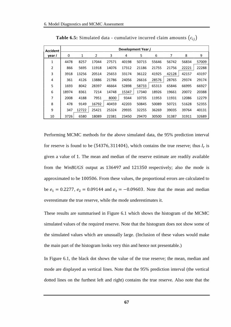
6. Model Diagnostics and MCMC Assessment
67
Table 6.5: Simulated data - cumulative incurred claim amounts
Accident year i
Development Year j
0 1 2 3 4 5 6 7 8 9
1 4478 8257 17044 27571 40198 50715 55646 56742 56834 57009
2 866 5695 11918 14076 17312 21186 21755 21756 22221 22288
3 3918 13256 20514 25653 33174 36122 41925 42128 42157 43197
4 361 4126 13886 21786 24056 26616 28576 28765 29374 29174
5 1693 8042 28397 46664 52898 58733 65313 65846 66995 66927
6 18974 8361 7214 14748 15347 17340 18926 19661 20072 20388
7 2008 4188 7951 8000 9344 10735 11953 11931 12086 12279
8 478 9149 16792 40459 42203 50845 50089 50721 51628 52355
9 347 12722 25421 25324 29935 32255 36269 39035 39764 40131
10 3726 6580 18089 22381 23450 29470 30500 31387 31911 32689
Performing MCMC methods for the above simulated data, the 95% prediction interval
for reserve is found to be , which contains the true reserve; thus is
given a value of . The mean and median of the reserve estimate are readily available
from the WinBUGS output as and respectively; also the mode is
approximated to be . From these values, the proportional errors are calculated to
be , and . Note that the mean and median
overestimate the true reserve, while the mode underestimates it.
These results are summarised in Figure 6.1 which shows the histogram of the MCMC
simulated values of the required reserve. Note that the histogram does not show some of
the simulated values which are unusually large. (Inclusion of these values would make
the main part of the histogram looks very thin and hence not presentable.)
In Figure 6.1, the black dot shows the value of the true reserve; the mean, median and
mode are displayed as vertical lines. Note that the 95% prediction interval (the vertical
dotted lines on the furthest left and right) contains the true reserve. Also note that the

6. Model Diagnostics and MCMC Assessment
68
mode corresponds to the highest point of the non-parametric density for the predicted
reserve.
Figure 6.1: Frequency histogram of simulated reserve
On average, a 95% prediction interval should be able to capture the true quantity with a
probability of . However, in this complicated model the 95% prediction interval
cannot be determined exactly, and has to be estimated via MCMC methods; this raises a
question on how well does the 95% prediction interval estimated with MCMC methods
represent the exact 95% prediction interval. The MCMC estimate of the 95% prediction
interval can be assessed by determining the true coverage of the prediction interval; this
is achieved by performing the MCMC methods again and again each time to a different
set of simulated run-off triangle.
Denote as the coverage of the MCMC 95% prediction interval. is defined to be the
proportion of the 95% prediction intervals containing the true reserve:

6. Model Diagnostics and MCMC Assessment
69
Note that the superscript represents the iteration number.
It is important to determine if the point estimates of the required reserve are reasonably
close to the true reserve. Due to the random nature of the claims, it is certain that the
estimates will be higher or lower than the true reserve. However, hopefully on average,
the positive deviations and the negative deviations will even out. The accuracy of the
estimates will be assessed by calculating the biases, denoted by and for mean,
median and mode respectively.
Define the bias as the average of the proportional errors:
Proportional error is chosen instead of absolute error because the true reserve for each
iteration can be very large or very small, for which the absolute errors will be distorted
by the size of the true reserve. For example, if the true reserve is very large, the absolute
error will be very large hence this particular absolute error is not comparable to that of
other iterations.
After performing MCMC predictions with WinBUGS in R (see the
implementation code in Appendix B-9), the coverage is found to be with
confidence interval which contains . This suggests that the MCMC‟s
95% prediction interval is a good approximation to the exact 95% prediction interval.
Note that the coverage is itself an approximation, meaning that the true coverage
might not be % (but there is 95% confidence that the true coverage is between
% and %).

6. Model Diagnostics and MCMC Assessment
70
Bias of the estimates are found to be , and
for mean, median and mode respectively. It appears that the usual MCMC prediction
(the mean) tends to overestimate the true reserve by % on average, while the median
only overestimates the true reserve by % on average and the mode underestimates the
true reserve only by a relatively small percentage ( %). Note that the mean is likely to
be affected by a couple of unusually large simulated values of reserve in MCMC
sampling whereas the median and mode are not; Figure 6.1 shows that the reserve is
positively skewed, hence it is very likely that there are some extremely large simulated
values for some of the iterations.
From the above results, one should ask whether the median is a more suitable choice for
reserving purposes than the mean, since the median is better in predicting the true
reserve compared to the mean. The mode tends to underestimate the required reserve;
hence it is not so suitable for reserving purposes. In practice, the reserve should never
be less than expected claims. As discussed in Chapter 2, the mean minimises the
quadratic error loss function, the median minimises the absolute error loss function and
the mode minimises the zero-one error loss function. Hence, if one wishes to be
conservative, the mean is the most appropriate for reserving purposes; however, the
median is also of value.
In conclusion, the reserve assessment in this section suggests that the MCMC approach
taken in this thesis works fairly well.

71
CHAPTER 7
CCoommppaarr iissoonn ttoo PPrreevviioouuss SSttuuddiieess
As mentioned above, the AFG Data were considered by Mack (1994), England and
Verrall (2002), and de Jong (2004); these data were analysed using the chain-ladder
method, a Bayesian over-dispersed Poisson model, and a classical development
correlation model, respectively. The forecasted liabilities for reserving purpose derived
from these models will be compared with the predicted reserve discussed in the thesis.
Table 7.1 shows the central estimates of the forecasted liabilities and their standard
errors associated with the above-mentioned models, together with the result from the
Bayesian implementation of the development correlation model discussed in Chapter 5.
Table 7.1: Forecasted liabilities for the AFG data
Accident Year
Chain Ladder Method
Bayesian Poisson Model
Classical Development
Correlation Model
Bayesian Development
Correlation Model
2 154 (206) 243 (486) 154 (146) 171 (155)
3 617 (623) 885 (984) 642 (375) 657 (431)
4 1,636 (753) 2,033 (1,589) 1,701 (753) 1,624 (895)
5 2,747 (1,456) 3,582 (2,216) 2,843 (1,271) 3,109 (1,504)
6 3,649 (2,007) 3,849 (2,301) 3,948 (1,462) 3,633 (1,627)
7 5,435 (2,228) 5,393 (2,873) 5,941 (2,290) 5,569 (2,421)
8 10,907 (5,344) 11,091 (4,686) 12,243 (5,463) 12,530 (5,784)
9 10,650 (6,284) 10,568 (5,563) 12,475 (6,747) 12,700 (7,288)
10 16,339 (24,509) 17,654 (12,801) 22,957 (11,551) 23,940 (14,060)
Total 52,135 (26,909) 55,297 (17,357) 62,982 (16,260) 63,930 (18,900)
The forecasted liabilities derived from the Bayesian development correlation model are
of similar scale compared to the others, especially the classical development correlation
model, while the standard errors associated with each accident year are greater than
their classical counterparts.

7. Comparison to Previous Studies
72
Note that generally the classical approach tends to underestimate the variability of the
parameters, especially when the data are scarce. For instance, when only a single data
point is present, the classical approach of de Jong (2004) effectively estimates the
variance as zero (see Table 5.1), whereas the Bayesian approach estimates the variance
as infinite; similar treatment was applied to the development factor associated with the
last column of the claim run-off triangle (the highest development year). Besides, in the
classical development correlation model, de Jong did not take account of the
uncertainties in parameter estimation, the standard errors derived (see Table 7.1) only
account for the uncertainties in prediction.
Also note that the total liability is the sum of the forecasted liabilities associated with
each accident year. Subject to rounding errors, the total liabilities shown in Table 7.1
are consistent with the sum of the individual liabilities for all models except for the
classical development correlation model, for which they differ by ; this might
be due to a possible fault associated with the prediction method used in the classical
development correlation model. For the Bayesian development correlation model, the
total liability differs from the sum by ; this is because the estimates are rounded
to the nearest 4 significant figures in WinBUGS.

73
CHAPTER 8
SSuummmmaarryy aanndd DDiissccuussssiioonn
8.1 Limitations of the Bayesian development correlation model
Note that to facilitate comparison, the required reserve in the model is determined
before discounting. In practice, the actual reserve held is the discounted outstanding
claims liabilities plus any adjustment. Albeit tedious, it is easy and straightforward to
incorporate discounting into the model; this can be achieved by calculating each claim
liability (not the cumulative claim liability) associated with the lower claim run-off
triangle and discounting it accordingly. The discount factors have to be explicitly
assumed; they can be either fixed for each year or vary across the calendar years.
Treatment of discounting the liabilities can be seen in Scollnik (2004).
Another limitation is that inflation rates are not explicitly considered in the model. If
inflation is assumed to be known, it can be incorporated into the model by first adjusting
the AFG Data. Then the same modelling technique discussed in previous chapters can
be applied to the adjusted AFG Data, and the claims liabilities can be inflated in the
same way as how the discount factors apply.
If the inflation rates are not known and need to be estimated from the data, the whole
modelling procedure becomes much more difficult; this is because the inflation rates are
partly captured by the development correlation factors and the structure of the inflation
rates need to be understood so that the inflation rates can be determined. Inflation is not
incorporated in the model due to lack of data; estimation of inflation would reduce the
accuracy and precision of other parameter estimates.

8. Summary and Discussion
74
8.2 Suggestions for future research
The Bayesian development correlation model from Section 5.3 could be improved by
incorporating discount rates and inflation rates as discussed in the previous section. This
would give a more realistic model to be used for reserving purposes. If inflation rates
are estimated from the model, care must be taken to ensure that the inflation rates are
sensible, especially when the data are scarce.
Extensions to the model suggested by de Jong were discussed in Section 4.2. As only
one of the extensions is implemented in the thesis, the other two are left for future
research. These extensions are the accident correlation model and the calendar
correlation model which incorporate correlation across accident years and calendar
years, respectively.
8.3 Conclusion
This thesis has explored a Bayesian analysis of three models: Hertig‟s (1985) model, a
modification of that model, and de Jong‟s (2004) development correlation model.
Outstanding claims liabilities associated with a claim run-off triangle, known as the
AFG Data, were forecasted for reserving purposes, using MCMC simulations generated
with WinBUGS.
Of these three models, the development correlation model is selected as the best for
reserving purposes. This judgement is based on model diagnostics and the reserve
assessments discussed in Chapter 6.

8. Summary and Discussion
75
The estimated reserve from this „best‟ model is then compared to the estimated reserve
obtained using the chain-ladder method (Mack, 1993), a Bayesian over-dispersed
Poisson model (England & Verrall, 2002), and the classical development correlation
model (de Jong, 2004) in Chapter 7. It is concluded that the Bayesian development
correlation model provides a better estimation of outstanding claim reserve than the
classical development correlation model.

76
BBiibbll iiooggrraapphhyy
Bornhuetter, R. L., & Ferguson, R. E. (1972). The Actuary and IBNR. Proceedings of
the Casualty Actuarial Society, LIX, 181-185.
de Alba, E. (2002). Bayesian Estimation of Outstanding Claim Reserves. North
American Actuarial Journal, 6(4), 1-1-20.
de Alba, E. (2006). Claims Reserving When There Are Negative Values in the Runoff
Triangle: Bayesian analysis using the three-parameter log-normal distribution.
North American Actuarial Journal, 10(3), 45-45-59.
de Alba, E., & Nieto-Barajas, L. E. (2008). Claims reserving: a correlated Bayesian
model. Insurance mathematics and economics, 43(3), 368-368-376. doi:
10.1016/j.insmatheco.2008.05.007
de Jong, P. (2004). Forecasting general insurance liabilities. Research paper, 2004/03,
Macquarie University.
England, P. D., & Verrall, R. J. (2002). Stochastic Claims Reserving in General
Insurance. British Actuarial Journal, 8(3), 443-443-518. doi:
10.1017/s1357321700003809
England, P. D., Verrall, R. J., & Wuthrich, M. V. (2010). Bayesian overdispersed
Poisson model and the Bornhuetter-Ferguson claims reserving method.
Retrieved from http://www.math.ethz.ch/~wueth/Papers/2010_ODP_BF.pdf
Gelman, A., Carlin, J., Stern, H., & Rubin, D. (2003). Bayesian Data Analysis. CRC
Press, Boca Raton, second edition.
Harnek, R. F. (1966). Formula Loss Reserves. Insurance Accounting and statistical
Proceedings.

Bibliography
77
Hastings, W. K. (1970). Monte Carlo Sampling Methods Using Markov Chains and
Their Applications. Biometrika, 57(1), 97-109.
Hertig, J. (1985). A Statistical Approach to IBNR-Reserves in Marine Reinsurance.
Astin Bulletin, 15(2), 171-183. doi: 10.2143/AST.15.2.2015027
Hobert, J. P., & Casella, G. (1996). The Effect of Improper Priors on Gibbs Sampling in
Hierarchical Linear Mixed Models. Journal of the American Statistical
Association, 91(436), 1461-1473.
Lamps, D. (2002a). An Application of Markov Chain Monte Carlo Theory to Claim Run
Off Analysis. Paper presented at the Annual Meeting of the Society of Actuaries,
Boston, Massachusetts, October 27-30, 2002.
Lamps, D. (2002b). Bayesian Analysis of Claim Lag Data Using WinBUGS Software.
Paper presented at the Annual Meeting of the Society of Actuaries, Boston,
Massachusetts, October 27-30, 2002.
Lamps, D. (2002c). A Set of Bayesian Models for Analysis of Claim Lags. Actuarial
Research Clearing House, 2003(1).
Lunn, D. J., Thomas, A., Best, N., & Spiegelhalter, D. (2000). WinBUGS - A Bayesian
modelling framework: Concepts, structure, and extensibility. Statistics and
Computing, 10(4), 325-337. doi: 10.1023/a:1008929526011
Mack, T. (1993). Distribution-free calculation of the standard error of chain ladder
reserves estimates. ASTIN Bulletin, 23(2), 213-225.
Mack, T. (1994). Measuring the Variability of Chain Ladder Reserve Estimates. In
Proceedings of the Casualty Actuarial Society Spring Forum, 101-182.
Mack, T. (2006). Chain-Ladder Method Encyclopedia of Actuarial Science: John Wiley
& Sons, Ltd.

Bibliography
78
McKeague, I. W., & Wefelmeyer, W. (2000). Markov chain Monte Carlo and Rao–
Blackwellization. Journal of Statistical Planning and Inference, 85(1-2), 171-
182. doi: 10.1016/s0378-3758(99)00079-8
Merkle, E., & Zandt, T. (2005). WinBUGS Tutorial Outline. Retrieved from
http://psychology.wichita.edu/merkle/tools/winbugsho.pdf
Metropolis, N., Rosenbluth, A. W., Rosenbluth, M. N., Teller, A. H., & Teller, E.
(1953). Equations of State Calculations by Fast Computing Machines. Journal
of Chemical Physics, 21(6), 1087-1092. doi: 10.1063/1.1699114
Pawlikowski, K. (1990). Steady-state simulation of queueing processes: A survey of
problems and solutions. ACM Computing Surveys, 22(2), 123-170.
Raftery, A. E., & Lewis, S. M. (1995). The number of iterations, convergence
diagnostics and generic Metropolis algorithms. Retrieved from
http://citeseerx.ist.psu.edu/viewdoc/download?doi=10.1.1.41.6352&rep=rep1&t
ype=pdf
Scollnik, D. P. M. (2004). Bayesian reserving models inspired by chain-ladder methods
and implemented using WinBUGS. ARCH, 2004(2).
Sheu, C.-F., & O'Curry, S. L. (1998). Simulation-based Bayesian inference using BUGS.
Behavior Research Methods, Instruments, and Computers, 30, 232-237.
Spiegelhalter, D. J., Thomas, A., Best, N., & Lunn, D. (2003). WinBUGS user manual,
version 1.4. MRC Biostatistics Unit, Cambridge, UK.
Taylor, G. (2000). Loss reserving. An actuarial perspective: Boston: Kluwer.
Verrall, R. J. (1990). Bayes and Empirical Bayes Estimation for the Chain Ladder
Model. ASTIN Bulletin, 20, 217-243.
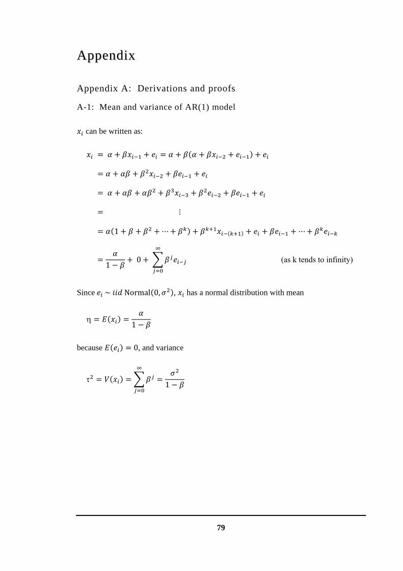
79
AAppppeennddiixx
Appendix A: Derivations and proofs
A-1: Mean and variance of AR(1) model
can be written as:
(as k tends to infinity)
Since , has a normal distribution with mean
because , and variance

Appendix
80
A-2: Derivation of expected values for Rao-Blackwell estimate
Since , the expected value of given
is . Conditioning on and :
More generally, for :

Appendix
81
A-3: Derivation of and
If random variables and are independent, with simple algebra, the variance of XY
can be written as followed:
Delta method:
Utilising the first order Taylor expansion, write . Letting
and , the expected value and variance can be
derived as:
If , then & , using the above result gives
For Hertig‟s basic model and its modification using the above results and independence
between and , the expected value and the variance of are:
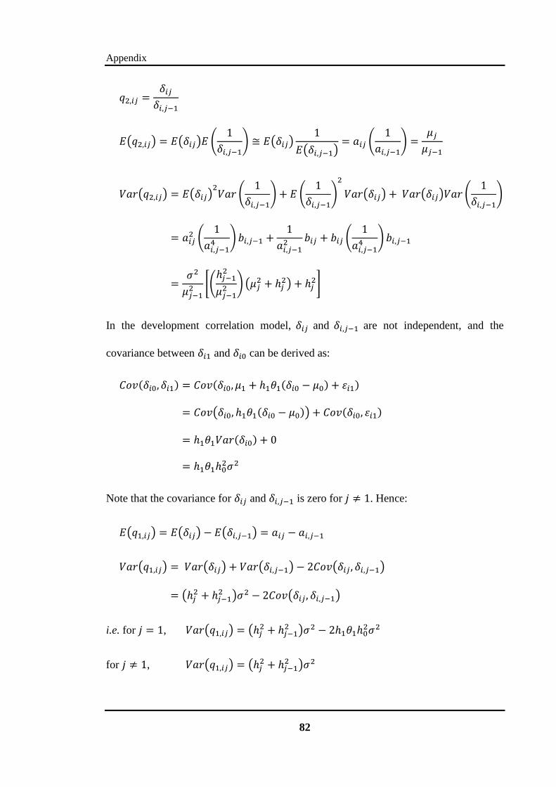
Appendix
82
In the development correlation model, and are not independent, and the
covariance between and can be derived as:
Note that the covariance for and is zero for . Hence:
i.e. for ,
for ,

Appendix
83
Appendix B: R code
B-1: Generation of time series values of
n <- 100
alpha.real <- 0.2
beta.real <- 0.6
sigma2.real <- 1
eta.real <- alpha.real/(1-beta.real)
tau2.real <- sigma2.real/(1-beta.real)
x1 <- rnorm(1,eta.real,sqrt(tau2.real))
xvec <- 1:n; xvec[1] <- x1
for(i in 2:n) {
xvec[i] <- rnorm(1,alpha.real+beta.real*xvec[i-1],sqrt(sigma2.real))
}
# Time Series of x (Figure 2.1)
X11(width=10,height=4); par(mfrow=c(1,1)); par(mai=c(1,1,0.2,0.2))
plot(xvec,type="l",xlab="t",ylab=~x[t], cex.lab=1.7)
B-2: The MH algorithm
# log posterior density of theta
LOGPOSFUN <- function(alpha,beta,sigma2,x.vector) {
n <- length(x.vector)
logf.xi <- x.vector[2:n]
for(i in 2:n) {
logf.xi[i] <- -log(sigma2)/2 -((x.vector[i]-alpha-beta*x.vector[i-1])^2)/(2*sigma2)
}
eta <- alpha/(1-beta)
tau2 <- sigma2/(1-beta)
logf.x1 <- -log(tau2)/2 -((x.vector[1]-eta)^2)/(2*tau2)
logposfun <- -log(sigma2) + logf.x1 + sum(logf.xi)
logposfun
}
MH.TS <- function(alpha,beta,sigma2,a.tuning,b.tuning,s.tuning,xvec,burn=100,J=1000) {
alpha.vec <- alpha
beta.vec <- beta
sigma2.vec <- sigma2
alpha.count <- 0; beta.count <- 0; sigma2.count <- 0
n <- length(xvec)
for(i in 1:(burn+J)) {
alpha1 <- runif(1,alpha-a.tuning,alpha+a.tuning)
p <- exp(LOGPOSFUN(alpha1,beta,sigma2,xvec) - LOGPOSFUN(alpha,beta,sigma2,xvec))
if(runif(1) < p) {
alpha <- alpha1
alpha.count <- alpha.count + 1
}
beta1 <- runif(1,beta-b.tuning,beta+b.tuning)
if((beta1 < 1)&&(beta1 > -1)) {
p <- exp(LOGPOSFUN(alpha,beta1,sigma2,xvec) - LOGPOSFUN(alpha,beta,sigma2,xvec))
if(runif(1) < p) {
beta <- beta1
beta.count <- beta.count + 1
}
}
sigma21 <- runif(1,sigma2-s.tuning,sigma2+s.tuning)
if(sigma21 > 0) {
p <- exp(LOGPOSFUN(alpha,beta,sigma21,xvec) - LOGPOSFUN(alpha,beta,sigma2,xvec))
if(runif(1) < p) {
sigma2 <- sigma21
sigma2.count <- sigma2.count + 1
}
}

Appendix
84
alpha.vec <- c(alpha.vec,alpha)
beta.vec <- c(beta.vec,beta)
sigma2.vec <- c(sigma2.vec,sigma2)
}
alpha.ar <- alpha.count/(burn+J)
beta.ar <- beta.count/(burn+J)
sigma2.ar <- sigma2.count/(burn+J)
list(alpha.vec=alpha.vec, beta.vec=beta.vec, sigma2.vec=sigma2.vec,
alpha.ar=alpha.ar, beta.ar=beta.ar, sigma2.ar=sigma2.ar)
}
burn <- 100
J <- 1000
ts1 <- MH.TS(0,0,0.5,0.2,0.2,0.5,xvec,burn,J)
c(ts1$alpha.ar, ts1$beta.ar, ts1$sigma2.ar)
avec <- ts1$alpha.vec; bvec <- ts1$beta.vec; s2vec <- ts1$sigma2.vec
# Simulation Traces (Figure 2.2, 2.3, 2.4)
X11(width=10,height=5); par(mai=c(1,1.2,0.2,0.2))
plot(0:(burn+J),avec,type="l", ann=F)
title(xlab="i",ylab=~alpha[i], cex.lab=1.7, font.lab=6)
abline(v=burn,lty=4)
X11(width=10,height=5); par(mai=c(1,1.2,0.2,0.2))
plot(0:(burn+J),bvec,type="l", ann=F)
title(xlab="i",ylab=~beta[i], cex.lab=1.7, font.lab=6)
abline(v=burn,lty=4)
X11(width=10,height=5); par(mai=c(1,1.2,0.2,0.2))
plot(0:(burn+J),s2vec,type="l", ann=F)
title(xlab="i",ylab=expression(paste(sigma[i]^2)), cex.lab=1.7, font.lab=6)
abline(v=burn,lty=4)
B-3: Inference on posterior quantities
BURN <- function(vector,n) {
# return a vector after a burn-in of n
vector[-(1:(n+1))]
}
INF <- function(vector) {
# return the mean, 95% CI, 95% CPDR of vector
m <- mean(vector)
s2 <- var(vector)
n <- length(vector)
ci <- m + c(-1,1)*qnorm(0.975)*sqrt(s2/n)
cpdr <- quantile(vector,c(0.025,0.975))
names(m) <- "mean"
names(ci) <- c("lower","upper")
c(m,ci,cpdr)
}
INF2 <- function(vector,sub,showS2=F) {
# return the mean, 95% CI, 95% CPDR and sample variances
# CI is calculator in 2 ways: CI1: 'ordinary', CI2: 'batch means'
inf <- INF(vector)
m <- length(vector)/sub ## how many in a group
yv <- rep(NA,sub)
for(i in 1:sub) {
yv[i] <- mean(vector[(m*(i-1)+1):(m*i)])
}
s2.batch <- m*var(yv)
ci.batch <- inf[1] + c(-1,1)*qnorm(0.975)*sqrt(s2.batch/length(vector))
names(ci.batch) <- c("lower","upper")
result = c(inf[1:3],ci.batch,inf[4:5])
if(showS2) { result=c(result,"s2"=var(vector),"s2b"=s2.batch) }
result
}

Appendix
85
avec <- BURN(avec,burn); bvec <- BURN(bvec,burn); s2vec <- BURN(s2vec,burn)
evec <- avec/(1-bvec)
tvec <- s2vec/(1-bvec)
options(digits=4)
rbind(alpha=c(true=alpha.real,INF2(avec,20)),beta=c(true=beta.real,INF2(bvec,20)),
"sigma^2"=c(true=sigma2.real,INF2(s2vec,20)),
"eta"=c(true=eta.real,INF2(evec,20)),"tau^2"=c(true=tau2.real,INF2(tvec,20)))
# Frequency Histograms (Figure 2.5, 2.6, 2.7, 8.1, 8.2)
X11(width=8,height=4.5); par(mai=c(1,1.2,0.4,0.2))
hist(avec,prob=T,ylim=c(0,4),breaks=20,xlab=~alpha,ylab="relative frequency",main=NA)
lines(density(avec),lty=1); abline(v=INF2(avec,20),lty=3); points(alpha.real,0,pch=19)
X11(width=8,height=4.5); par(mai=c(1,1.2,0.2,0.2))
hist(bvec,prob=T,breaks=20,xlab=~beta,ylab="relative frequency",main=NA)
lines(density(bvec),lty=1); abline(v=INF2(bvec,20),lty=3); points(beta.real,0,pch=19)
X11(width=8,height=4.5); par(mai=c(1,1.2,0.2,0.2))
hist(s2vec,prob=T,breaks=20,xlab=expression(paste(sigma^2)),
ylab="relative frequency",main=NA)
lines(density(s2vec),lty=1); abline(v=INF2(s2vec,20),lty=3); points(sigma2.real,0,pch=19)
X11(width=8,height=4.5); par(mai=c(1,1.2,0.2,0.2))
hist(evec,prob=T,breaks=20,xlab=~eta,ylab="relative frequency",main=NA)
lines(density(evec),lty=1); abline(v=INF2(evec,20),lty=3); points(eta.real,0,pch=19)
X11(width=8,height=4.5); par(mai=c(1,1.2,0.4,0.2))
hist(tvec,prob=T,breaks=20,xlab=expression(paste(tau^2)),
ylab="relative frequency",main=NA)
lines(density(tvec),lty=1); abline(v=INF2(tvec,20),lty=3); points(tau2.real,0,pch=19)
B-4: Predictive inference
M <- 10
lastx <- xvec[length(xvec)]; lastx
xs.matrix <- matrix(NA,nrow=M,ncol=J)
for(i in 1:J) {
xs.matrix[1,i] <- rnorm(1,avec[i]+bvec[i]*lastx,sqrt(s2vec[i]))
for(m in 2:M) {
xs.matrix[m,i] <- rnorm(1,avec[i]+bvec[i]*xs.matrix[m-1,i],sqrt(s2vec[i]))
}
}
xs.inf <- matrix(NA,nrow=M,ncol=9)
xs.name <- rep(NA,M)
for(m in 1:M) {
xs.inf[m,] <- INF2(xs.matrix[m,],20,showS2=T)
xs.name[m] <- paste("x(n+",m,")",sep="")
}
label <- names(INF2(1,1,showS2=T))
dimnames(xs.inf) <- list(xs.name,label)
options(digits=3)
xs.inf
X11(width=8,height=5); par(mai=c(1,1,0.2,0.2)) # (Figure 2.8)
plot(xs.inf[,1],ylim=range(xs.inf[,4:5]),type="l",
xlab="t",ylab="Forecasted mean of " ~x[n+t])
abline(h=mean(evec),lty=2)
lines(xs.inf[,2],lty=3); lines(xs.inf[,3],lty=3)
lines(xs.inf[,4],lty=4); lines(xs.inf[,5],lty=4)
lines(xs.inf[,6],lty=8); lines(xs.inf[,7],lty=8)
legend(5,-0.2,c("mean","ordinary CI","batch means CI",
"estimated post. mean"),lty=c(1,3,4,2))
xs.range <- range(xs.matrix)
xs.min <- floor(xs.range[1])
xs.max <- ceiling(xs.range[2])

Appendix
86
X11(width=8,height=4.5); par(mai=c(1,1.2,0.4,0.2)) # (Figure 2.10)
hist(xs.matrix[m,],prob=T,breaks=20,xlab=~x[n+10],ylab="relative frequency",main=NA)
lines(density(xs.matrix[k,]),lty=1); abline(v=xs.inf[k,][-(8:9)],lty=3);
points(mean(evec),0,pch=19)
# Rao Blackwell approach
xs.matrix2 <- matrix(NA,nrow=M,ncol=J)
for(i in 1:J) {
xs.matrix2[1,i] <- avec[i]+bvec[i]*lastx
for(m in 2:M) {
xs.matrix2[m,i] <- avec[i]+bvec[i]*xs.matrix2[m-1,i]
}
}
xs.inf <- matrix(NA,nrow=M,ncol=5)
xs.name <- rep(NA,M)
for(m in 1:M) {
xs.inf[m,] <- INF2(xs.matrix2[m,],20)[1:5]
xs.name[m] <- paste("x(n+",m,")",sep="")
}
label <- names(INF2(1,1)[1:5])
dimnames(xs.inf) <- list(xs.name,label)
xs.inf
X11(width=8,height=5); par(mai=c(1,1,0.2,0.2)) # (Figure 2.9)
plot(xs.inf[,1],ylim=range(xs.inf[,4:5]),type="l",
xlab="t",ylab="Estimated mean of " ~x[n+t])
abline(h=mean(evec),lty=2)
lines(xs.inf[,2],lty=3); lines(xs.inf[,3],lty=3)
lines(xs.inf[,4],lty=4); lines(xs.inf[,5],lty=4)
legend(4.5,-0.1,c("mean","ordinary CI","batch means CI",
"estimated post. mean"),lty=c(1,3,4,2))
B-5: Hypothesis testing
RUN.COUNT <- function(xvec,mid=mean(xvec)) {
# this function counts the number of runs above or below 'mid'
xvec <- xvec - mid
sign <- sign(xvec[1])
count <- 1
for(i in 2:length(xvec)) {
if(sign(xvec[i]) != sign) {
sign <- sign(xvec[i])
count <- count + 1
}
}
count
}
LOGPOSFUN2 <- function(alpha,sigma2,x.vector) {
n <- length(x.vector)
logf.xi <- rep(NA,n)
for(i in 1:n) {
logf.xi[i] <- -log(sigma2)/2 -((x.vector[i]-alpha)^2)/(2*sigma2)
}
logposfun <- -log(sigma2) + sum(logf.xi)
logposfun
}
MH.TS2 <- function(alpha,sigma2,a.tuning,s.tuning,xvec,burn=100,J=1000) {
alpha.vec <- alpha
sigma2.vec <- sigma2
alpha.count <- 0; sigma2.count <- 0
n <- length(xvec)
for(i in 1:(burn+J)) {
alpha1 <- runif(1,alpha-a.tuning,alpha+a.tuning)
p <- exp(LOGPOSFUN2(alpha1,sigma2,xvec) - LOGPOSFUN2(alpha,sigma2,xvec))
if(runif(1) < p) {

Appendix
87
alpha <- alpha1
alpha.count <- alpha.count + 1
}
sigma21 <- runif(1,sigma2-s.tuning,sigma2+s.tuning)
if(sigma21 > 0) {
p <- exp(LOGPOSFUN2(alpha,sigma21,xvec) - LOGPOSFUN2(alpha,sigma2,xvec))
if(runif(1) < p) {
sigma2 <- sigma21
sigma2.count <- sigma2.count + 1
}
}
alpha.vec <- c(alpha.vec,alpha)
sigma2.vec <- c(sigma2.vec,sigma2)
}
alpha.ar <- alpha.count/(burn+J)
sigma2.ar <- sigma2.count/(burn+J)
list(alpha.vec=alpha.vec,sigma2.vec=sigma2.vec, alpha.ar=alpha.ar,sigma2.ar=sigma2.ar)
}
burn <- 200
J <- 10000
xlist <- c(100)
ppp1 <- rep(NA,length(xlist)); ppp2 <- ppp1
for(j in 1:length(xlist)) {
new.xvec <- xvec[1:xlist[j]]
n <- length(new.xvec)
ts <- MH.TS2(0,1,0.3,0.5,xvec,burn,J)
avec2 <- BURN(ts$alpha.vec,burn); s2vec2 <- BURN(ts$sigma2.vec,burn)
indicator1 <- rep(0,J)
for(i in 1:J) {
xrep <- rnorm(n,avec2[i],sqrt(s2vec2[i]))
T1 <- RUN.COUNT(xrep,avec2[i])
T0 <- RUN.COUNT(new.xvec,avec2[i])
if(T1 <= T0) { indicator1[i] <- 1 }
}
ppp1[j] <- sum(indicator1)/J
indicator2 <- rep(0,J)
T0 <- RUN.COUNT(new.xvec)
for(i in 1:J) {
xrep <- rnorm(n,avec2[i],sqrt(s2vec2[i]))
T1 <- RUN.COUNT(xrep)
if(T1 <= T0) { indicator2[i] <- 1 }
}
ppp2[j] <- sum(indicator2)/J
}
cbind('m'=xlist,ppp1,ppp2)
B-6: Approximation of exact posterior densities
INTEG <- function(xvec,yvec,a=min(xvec),b=max(xvec)) {
# Integrates numerically under a spline through the points given by
# the vectors xvec and yvec, from a to b.
fit <- smooth.spline(xvec, yvec)
spline.f <- function(x){ predict(fit, x)$y }
integrate(spline.f, a, b)$value
}
D.integrate <- function(fxy,xlower,xupper,ylower,yupper,...,precision=0.02) {
# Perform double integration on the function fxy
yvec <- seq(ylower,yupper,precision)
gy <- rep(NA,length(yvec)) # integrand of fxy with respect to x
for(i in 1:length(yvec)) {
xvec <- seq(xlower,xupper,precision)
gx <- rep(NA,length(xvec))
for(j in 1:length(xvec)) {
gx[j] <- fxy(xvec[j],yvec[i],...)

Appendix
88
}
gy[i] <- INTEG(xvec,gx,xlower,xupper)
}
INTEG(yvec,gy,ylower,yupper)
}
alpha.values <- seq(-5,1,0.02)
poskern.alpha <- rep(NA,length(alpha.values))
for(i in 1:length(alpha.values)) {
fxy <- function(sigma2,beta) { exp(LOGPOSFUN(alpha.values[i],beta,sigma2,xvec)) }
poskern.alpha[i] <- D.integrate(fxy,0.09,20,-0.99,0.99,precision=0.09)
plot(alpha.values[i],0,xlim=range(alpha.values)) # for checking the progress
}
pos.alpha <- poskern.alpha/(INTEG(alpha.values,poskern.alpha))
pos.mean.alpha <- INTEG(alpha.values,alpha.values*pos.alpha)
pos.mean.alpha # 0.0812
pos.var.alpha <- INTEG(alpha.values,((alpha.values-pos.mean.alpha)^2)*pos.alpha)
pos.var.alpha # 0.0110
X11(width=8,height=5); par(mai=c(1,1,0.2,0.2)) # (Figure 2.11)
plot(alpha.values,pos.alpha,type="l",xlim=c(-1,1),xlab=~alpha,ylab="density",main=NA)
lines(density(avec),lty=3); abline(v=pos.mean.alpha,lty=2); legend(-1,3,c("approximated
exact density","non-parametric density","posterior mean"),lty=c(1,3,2))
beta.values <- seq(-0.98,0.98,0.02)
poskern.beta <- rep(NA,length(beta.values))
for(i in 1:length(beta.values)) {
fxy <- function(sigma2,alpha) { exp(LOGPOSFUN(alpha,beta.values[i],sigma2,xvec)) }
poskern.beta[i] <- D.integrate(fxy,0.1,20,-1,1,precision=0.1)
plot(beta.values[i],0,xlim=range(beta.values)) # for checking the progress
}
pos.beta <- poskern.beta/(INTEG(beta.values,poskern.beta))
pos.mean.beta <- INTEG(beta.values,beta.values*pos.beta)
pos.mean.beta # 0.56
pos.var.beta <- INTEG(beta.values,((beta.values-pos.mean.beta)^2)*pos.beta)
pos.var.beta # 0.00721
X11(width=8,height=5); par(mai=c(1,1,0.2,0.2)) # (Figure 2.12)
plot(beta.values,pos.beta,type="l",xlab=~beta,ylab="density",main=NA)
lines(density(bvec),lty=3); abline(v=pos.mean.beta,lty=2); legend(-0.75,3,
c("approximated exact density","non-parametric density","posterior mean"),lty=c(1,3,2))
sigma2.values <- seq(0.02,4,0.02)
poskern.sigma2 <- rep(NA,length(sigma2.values))
for(i in 1:length(sigma2.values)) {
fxy <- function(alpha,beta) { exp(LOGPOSFUN(alpha,beta,sigma2.values[i],xvec)) }
poskern.sigma2[i] <- D.integrate(fxy,-1,1,-0.99,0.99,precision=0.09)
plot(sigma2.values[i],0,xlim=range(sigma2.values)) # for checking the progress
}
pos.sigma2 <- poskern.sigma2/(INTEG(sigma2.values,poskern.sigma2))
pos.mean.sigma2 <- INTEG(sigma2.values,sigma2.values*pos.sigma2)
pos.mean.sigma2 # 1.05
pos.var.sigma2 <- INTEG(sigma2.values,((sigma2.values-pos.mean.sigma2)^2)*pos.sigma2)
pos.var.sigma2 # 0.0235
X11(width=8,height=5); par(mai=c(1,1,0.2,0.2)) # (Figure 2.13)
plot(sigma2.values,pos.sigma2,type="l",ylim=c(0,2.85),xlab=expression(paste(sigma^2)),
ylab="density",main=NA)
lines(density(s2vec),lty=3); abline(v=pos.mean.sigma2,lty=2); legend(2,2,c("approximated
exact density","non-parametric density","posterior mean"),lty=c(1,3,2))
B-7: Coverage assessment
m <- 10
trial <- 1000
I <- rep(0,trial); Ib <- Is <- rep(0,trial)
data <- matrix(NA,nrow=trial,ncol=3); xrep <- matrix(NA,nrow=m,ncol=J)
for(i in 1:trial) {

Appendix
89
x1 <- rnorm(1,eta.real,sqrt(tau2.real))
xvec <- rep(NA,n); xvec[1] <- x1
for(j in 2:(n+m)) {
xvec[j] <- rnorm(1,alpha.real+beta.real*xvec[j-1],sqrt(sigma2.real))
}
ts1 <- MH.TS(0,0,0.5,0.25,0.25,0.5,xvec[1:n],burn,J)
avec <- ts1$alpha.vec; avec <- BURN(avec,burn)
aCI <- INF(avec)[4:5]
if((alpha.real>aCI[1])&&(alpha.real<aCI[2])) { I[i] <- 1 }
bvec <- BURN(ts1$beta.vec,burn); bCI <- INF(bvec)[4:5]
if((beta.real>bCI[1])&&(beta.real<bCI[2])) { Ib[i] <- 1 }
s2vec <- BURN(ts1$sigma2.vec,burn); sCI <- INF(s2vec)[4:5]
if((sigma2.real>sCI[1])&&(sigma2.real<sCI[2])) { Is[i] <- 1 }
xmean <- rep(NA,m)
for(j in 1:J) {
xrep[1,j] <- rnorm(1,avec[j]+bvec[j]*xvec[n],sqrt(s2vec[j]))
for(k in 2:m) {
xrep[k,j] <- rnorm(1,avec[j]+bvec[j]*xrep[k-1,j],sqrt(s2vec[j]))
}
xmean[j] <- mean(xrep[,j])
}
PI <- INF(xmean)[4:5]
data[i,] <- c(mean(xvec[(n+1):(n+m)]),PI)
}
p = sum(I/trial); p # 0.947
p + c(-1,1)*qnorm(0.975)*sqrt(p*(1-p)/trial) # 0.9331145 0.9608855
pb = sum(Ib/trial); pb # 0.942
pb + c(-1,1)*qnorm(0.975)*sqrt(pb*(1-pb)/trial) # 0.9275127 0.9564873
ps = sum(Is/trial); ps # 0.938
ps + c(-1,1)*qnorm(0.975)*sqrt(ps*(1-ps)/trial) # 0.923 0.953
I1 <- I2 <- rep(NA,trial)
for(i in 1:trial) {
I1[i] <- ( data[i,1] > data[i,2] ) && ( data[i,1] < data[i,3] )
xvec <- rep(NA,n)
xvec[1] <- x1
for(j in 2:(n+m)) {
xvec[j] <- rnorm(1,alpha.real+beta.real*xvec[j-1],sqrt(sigma2.real))
}
xmean <- mean(xvec[(n+1):(n+m)])
I2[i] <- ( xmean > data[i,2] ) && ( xmean < data[i,3] )
}
p1 <- mean(I1); p2 <- mean(I2); c(p1,p2) # 0.933 0.918
p1 + c(-1,1)*qnorm(0.975)*sqrt(p1*(1-p1)/trial) # 0.9175 0.9485
p2 + c(-1,1)*qnorm(0.975)*sqrt(p2*(1-p2)/trial) # 0.901 0.935
B-8: Coverage assessment with WinBUGS
library("R2WinBUGS")
I <- rep(0,trial)
data <- matrix(NA,nrow=trial,ncol=3)
for(i in 1:trial) {
x1 <- rnorm(1,eta.real,sqrt(tau2.real))
x <- rep(NA,n); x[1] <- x1
for(j in 2:n) {
x[j] <- rnorm(1,alpha.real+beta.real*x[j-1],sqrt(sigma2.real))
}
xrep <- rep(NA,m)
xrep[1] <- rnorm(1,alpha.real+beta.real*x[n],sqrt(sigma2.real))
for(j in 2:m) {
xrep[j] <- rnorm(1,alpha.real+beta.real*xrep[j-1],sqrt(sigma2.real))
}

Appendix
90
# MCMC via winbugs
bugdata <- list("n","x","m")
buginits <- function() { list( beta=0, sigma2=1) }
bugparameters <- c("alpha","xmean")
bugsim <- bugs(bugdata, buginits, bugparameters, model.file=
"C:/Users/Carlo/Documents/R/Q1Predict.txt",
n.chains = 1, n.iter = J+burn, n.burnin = burn, DIC = FALSE,
bugs.directory = "C:/Program Files/WinBUGS14/",
working.directory = "C:/Users/Carlo/Documents/R/Q1/")
aCI <- c(bugsim$summary[1,3], bugsim$summary[1,7])
if((alpha.real>aCI[1])&&(alpha.real<aCI[2])) { I[i] <- 1 }
PI <- c(bugsim$summary[2,3], bugsim$summary[2,7])
data[i,] <- c(mean(xrep),PI)
}
p = sum(I/trial); p # 0.937
p + c(-1,1)*qnorm(0.975)*sqrt(p*(1-p)/trial) # 0.9219413 0.9520587
I1 <- I2 <- rep(NA,trial)
for(i in 1:trial) {
I1[i] <- ( data[i,1] > data[i,2] ) && ( data[i,1] < data[i,3] )
xvec <- rep(NA,n)
xvec[1] <- x1
for(j in 2:(n+m)) {
xvec[j] <- rnorm(1,alpha.real+beta.real*xvec[j-1],sqrt(sigma2.real))
}
xmean <- mean(xvec[(n+1):(n+m)])
I2[i] <- ( xmean > data[i,2] ) && ( xmean < data[i,3] )
}
p1 <- mean(I1); p2 <- mean(I2); c(p1,p2) # 0.926 0.903
p1 + c(-1,1)*qnorm(0.975)*sqrt(p1*(1-p1)/trial) # 0.9097756 0.9422244
p2 + c(-1,1)*qnorm(0.975)*sqrt(p2*(1-p2)/trial) # 0.8846567 0.9213433
B-9: Reserve assessment with WinBUGS
library("R2WinBUGS")
MODE <- function(vector) {
# estimate the mode from a density of vector by smoothing
den <- density(vector)
den$x[den$y==max(den$y)]
}
# parameters
year <- 10; n <- year; M <- 0.57; N <- 0.60
mu <- rep(0,n); mu[1:3] <- c(7.3, 1.5, 0.49)
h <- rep(0,n); h[1:3] <- c(1,0.21,0.22)
for(i in 4:n) {
mu[i] <- M^(i-3) * mu[3]
h[i] <- N^(i-3) * h[3]
}
theta <- -4.3; sigma2 <- 2.1
L <- 1000 # running the Gibbs sampler again and again for L times
I <- ppp.list <- error.mean <- error.median <- error.mode <- rep(0,L)
reserve.position <- 78; ppp.location <- 79; options(digits=4)
for(k in 1:L) {
# generating claim run off data
c <- matrix(NA, nrow=n, ncol=n)
delta <- matrix(NA, nrow=n, ncol=n)
for(i in 1:n) {
delta[i,1] <- rnorm(1, mu[1], h[1]*sqrt(sigma2))
delta[i,2] <- rnorm(1, mu[2]+h[2]*theta*(delta[i,1]-mu[1]), h[2]*sqrt(sigma2))
for(j in 3:n) {

Appendix
91
delta[i,j] <- rnorm(1, mu[j], h[j]*sqrt(sigma2))
}
}
for(i in 1:n) {
c[i,1] <- exp(delta[i,1])
for(j in 2:n) {
c[i,j] <- exp(delta[i,j]) * c[i,j-1]
}
}
true.reserve = 0
for(i in 2:n) {
true.reserve = true.reserve + (c[i,n] - c[i,11-i])
}
# MCMC
bugdata <- list("year","c")
buginits <- function() {
list( mu = c(0.1,0.1,0.1,NA,NA,NA,NA,NA,NA,NA), h = c(NA,1,1,NA,NA,NA,NA,NA,NA,NA),
M = 0.5 , N = 0.5 , sigma2 = 1, theta = 1, delta.rep = structure(.Data = c(
0, 0, 0, 0, 0, 0, 0, 0, 0, 0,
0, 0, 0, 0, 0, 0, 0, 0, 0,NA,
0, 0, 0, 0, 0, 0, 0, 0,NA,NA,
0, 0, 0, 0, 0, 0, 0,NA,NA,NA,
0, 0, 0, 0, 0, 0,NA,NA,NA,NA,
0, 0, 0, 0, 0,NA,NA,NA,NA,NA,
0, 0, 0, 0,NA,NA,NA,NA,NA,NA,
0, 0, 0,NA,NA,NA,NA,NA,NA,NA,
0, 0,NA,NA,NA,NA,NA,NA,NA,NA,
0,NA,NA,NA,NA,NA,NA,NA,NA,NA), .Dim = c(10,10) ))
}
Bugparameters <- c("mu","h","sigma2","M","N","theta",
"c.pred","reserve.part","reserve","p1","p3")
bugsim <- bugs(bugdata, buginits, bugparameters, model.file=
"C:/Users/xxxxx/Documents/R/Claim.txt",
n.chains = 1, n.iter = 11000, n.burnin = 1000, DIC = FALSE,
bugs.directory = "C:/Program Files/WinBUGS14/",
working.directory = "C:/Users/xxxxx/Documents/R/Claim/")
mean.reserve <- bugsim$mean$reserve; median.reserve <- bugsim$median$reserve
mode.reserve <- MODE(bugsim$sims.list$reserve)
PI.reserve <- c(bugsim$summary[reserve.position,3],bugsim$summary[reserve.position,7])
if((true.reserve > PI.reserve[1]) && (true.reserve < PI.reserve[2])) { I[l]=1 }
error.mean[l] <- (mean.reserve - true.reserve)/true.reserve
error.median[l] <- (median.reserve - true.reserve)/true.reserve
error.mode[l] <- (mode.reserve - true.reserve)/true.reserve
ppp.list <- bugsim$summary[ppp.location,1]
# progress tracking
if(l %% 10 == 0) { print(cat(l/L*100,"percent completed! ")) }
}
# Results
bugsim$summary[reserve.position,]; bugsim$mean$p1; bugsim$mean$p3
mode.reserve; true.reserve; p=mean(I); p; p + c(-1,1)*1.96*sqrt(p*(1-p)/L)
# Hypothesis testing
ppp.mean = mean(ppp.list); ppp.mean;
sum(ppp.mean[ppp.mean<0.05]); sum(ppp.mean[ppp.mean>0.95])
INF(error.mean)[1:3]; INF(error.median)[1:3]; INF(error.mode)[1:3]
reserve.vector <- bugsim$sims.list$reserve
X11(width=8,height=5); par(mai=c(1,1.2,0.2,0.2)) # (Figure 6.1)
hist(reserve.vector,breaks=40,prob=T,xlab="reserve",main=NA,xlim=c(min(reserve.vector),
quantile(reserve.vector,0.9975)))
abline(v=bugsim$summary[reserve.position,1],lty=1, lwd=2)
abline(v=bugsim$summary[reserve.position,5],lty=2, lwd=2)
abline(v=MODE(reserve.vector),lty=3, lwd=2); abline(v=PI.reserve,lty=4)
points(true.reserve,0,pch=19); lines(density(reserve.vector),lty=3);
legend(1.1*PI.reserve[2],0.5*max(density(reserve.vector)$y),c("mean","median","mode"),
lty=c(1,2,3),lwd=c(2,2,2))

Appendix
92
Appendix C: WinBUGS Code
C-1: Time series model
MODEL
{
x[1] ~ dnorm(eta,t)
for( i in 2 : n ) {
x[i] ~ dnorm(mu[i],s)
mu[i] <- alpha+beta*x[i-1]
}
t <- 1/tau2
s <- 1/sigma2
tau2 <- sigma2/(1-beta)
eta <- alpha/(1-beta)
alpha ~ dnorm(0,0.001)
beta ~ dunif(-1,1)
sigma2 ~ dgamma(0.001,0.001)
# Prediction
for( j in 1 : m) {
xnext[j] ~ dnorm(munext[j],s)
}
munext[1] <- alpha+beta*x[n]
for( j in 2 : m) {
munext[j] <- alpha+beta*xnext[j-1]
}
}
DATA
list(x =
c( -0.651134500293269, -1.13297671629464, 0.0902583995422782, -0.740492555568816,
0.713285477012912, 2.07994350899636, 1.45421438904982, 2.3381697281389,
1.37655363797294, 1.70107119781436, 0.721806461126196, -0.0219793729577730,
0.675082788161775, 1.23874412208321, -0.163227938659239, -1.03468020484809,
-1.2249661451836, -0.853068555277069, -1.73295486859530, -2.02798270492891,
-0.44366365835555, -0.305014271649753, 1.54102341989711, 1.96516193269735,
2.71260199074518, 1.49709675778887, 0.273603377570765, -0.577364695257764,
-0.421633068043591, 2.43096891928915, 0.691620566378797, 1.42058905389156,
-0.65768699060883, 0.460487372435315, 1.41358849385181, -0.892847049043457,
-1.29419561926962, -2.78297653575327, -2.21560748836394, 2.19632117391132,
1.02677193374616, 1.61495879538274, 3.19549635315063, 1.22857740530504,
1.60048437669280, 1.18059004472060, 1.26998139649821, 1.21220822584111,
0.12784681367819, -0.390724777992149, 0.841417275022684, -1.50778568978362,
-0.84289599914087, -1.4333697880734, -2.26213309168342, -1.02578547250705,
-0.0652596684436959, 0.227139857634588, -0.450604540675496, 0.39469840547178,
0.0226121794600207, -0.162096211508090, 0.00573523672703122, 0.78843378855997,
0.044661381446038, 0.94228199051853, 0.627176242272651, -0.0676376442225574,
-0.552602300807993, 1.71968604606597, 1.06298339935968, 0.376287370396052,
2.28118839342955, 2.32838018294078, 1.51419221969344, 0.359300452079709,
0.450986128926995, 0.285715539965825, 0.0634575029461997, -0.314828299900130,
0.143103691731009, -0.0699157299604746, -0.116372930898608, 0.561361459142413,
-1.18346979620212, -1.46430885733973, -0.0366906364238819, -0.928593920178746,
-1.17409023323741, 0.521128086916033, -1.34089457936068, -0.0515133312649343,
0.779648231613477, 1.35909656451904, -0.0656115327245324, 0.0084512260436784,
-1.44338475168051, -1.67820910177067, -0.979369032809375, -0.90346362304396),
xnext = c(NA,NA,NA,NA,NA,NA,NA,NA,NA,NA), n = 100, m = 15)
INITS
list( beta = 0, sigma2 = 1)

Appendix
93
C-2: Hypothesis testing on time series model
MODEL
{
for( i in 1 : n ) {
x[i] ~ dnorm(alpha,s)
}
s <- 1/sigma2
alpha ~ dnorm(0,0.001)
sigma2 ~ dgamma(0.001,0.001)
# Prediction
for( j in 1 : n) {
xrep[j] ~ dnorm(alpha,s)
}
# Hypothesis Test
mx <- mean(x[])
for( i in 1:m) {
y[i] <- (x[i] - mx) / abs(x[i] - mx)
}
for( i in 1:(m-1)) {
z[i] <- abs(y[i+1] - y[i]) / 2
}
xcount <- sum(z[]) + 1
mxrep <- mean(xrep[])
for( j in 1:m) {
yrep[j] <- (xrep[j] - mxrep) / abs(xrep[j] - mxrep)
}
for( j in 1:(m-1)) {
zrep[j] <- abs(yrep[j+1] - yrep[j]) / 2
}
xrepcount <- sum(zrep[]) + 1
ppp <- step(xcount – xrepcount)
}
DATA
# Same data as in Appendix C-1
INITS
list( sigma2 = 1)
C-3: Hertig‟s model (Section 5.1)
MODEL
{
for( i in 1 : year) {
delta[i,1] <- log( c[i,1] )
for( j in 2 : (year+1-i) ) {
delta[i,j] <- log( c[i,j] ) - log( c[i,j-1] )
}
for( j in 1 : (year+1-i) ) {
delta[i,j] ~ dnorm( mu.d[i,j], tau.d[i,j] )
mu.d[i,j] <- mu[j]
tau.d[i,j] <- 1 / ( pow(h[j],2) * sigma2 )
c.pred[i,j] <- 0
}
}
# Prior Distributions
for( j in 1 : year) {
mu[j] ~ dnorm(0,0.00001)
}
sigma2 ~ dgamma(0.1,0.1)
h[1] <- 1

Appendix
94
for( j in 2 : year) {
h[j] ~ dgamma(0.1,0.1)
}
# Prediction
for( i in 2 : year) {
delta[i,year+2-i] ~ dnorm( mu.d[i,year+2-i], tau.d[i,year+2-i])
mu.d[i,year+2-i] <- mu[year+2-i]
tau.d[i,year+2-i] <- 1 / ( pow(h[year+2-i],2) * sigma2 )
c.pred[i,year+2-i] <- c[i,year+1-i] * exp(delta[i,year+2-i])
}
for( i in 3 : year) {
for( j in (year+3-i) : year) {
delta[i,j] ~ dnorm( mu.d[i,j], tau.d[i,j] )
mu.d[i,j] <- mu[j]
tau.d[i,j] <- 1 / ( pow(h[j],2) * sigma2 )
c.pred[i,j] <- c.pred[i,j-1] * exp(delta[i,j])
}
}
reserve.part[1] <- 0
for( i in 2 : year) {
reserve.part[i] <- c.pred[i,year] - c[i,year+1-i]
}
reserve <- sum(reserve.part[])
# Hypothesis Test
for( i in 1 : year) {
for( j in 1 : (year+1-i) ) {
delta.rep[i,j] ~ dnorm( mu.d.rep[i,j], tau.d.rep[i,j] )
mu.d.rep[i,j] <- mu[j]
tau.d.rep[i,j] <- 1 / ( pow(h[j],2) * sigma2 )
}
}
for( i in 1 : (year-1) ) {
for( j in 2 : (year+1-i) ) {
Q1[i,j] <- delta[i,j] - delta[i,j-1]
Q2[i,j] <- delta[i,j] / delta[i,j-1]
Q1.rep[i,j] <- delta.rep[i,j] - delta.rep[i,j-1]
Q2.rep[i,j] <- delta.rep[i,j] / delta.rep[i,j-1]
mean.Q1[i,j] <- mu[j] - mu[j-1]
mean.Q2[i,j] <- mu[j] / mu[j-1]
var.Q1[i,j] <- ( pow(h[j],2) + pow(h[j-1],2) ) * sigma2
var.Q2[i,j] <- sigma2/pow(mu[j-1],2)*((pow(h[j-1],2)/pow(mu[j-1],2))
*(pow(mu[j],2) + pow(h[j],2)*sigma2) + pow(h[j],2) )
t1[i,j] <- pow(( Q1[i,j] - mean.Q1[i,j] ),2) / var.Q1[i,j]
t1.rep[i,j] <- pow(( Q1.rep[i,j] - mean.Q1[i,j] ),2) / var.Q1[i,j]
t2[i,j] <- pow(( Q2[i,j] - mean.Q2[i,j] ),2) / var.Q2[i,j]
t2.rep[i,j] <- pow(( Q2.rep[i,j] - mean.Q2[i,j] ),2) / var.Q2[i,j]
}
}
for( i in 1 : year ) {
t1[i,1] <- 0
t1.rep[i,1] <- 0
t2[i,1] <- 0
t2.rep[i,1] <- 0
}
for( i in 2 : year ) {
for( j in (year+2-i) : year ) {
t1[i,j] <- 0
t1.rep[i,j] <- 0
t2[i,j] <- 0
t2.rep[i,j] <- 0
}
}
Ts1 <- sum(t1[,])
Ts1.rep <- sum(t1.rep[,])
Ts2 <- sum(t2[,])
Ts2.rep <- sum(t2.rep[,])
p1 <- step( Ts1 - Ts1.rep ) # 1 if Ts1 >= Ts1.rep
p2 <- step( Ts2 - Ts2.rep ) # 1 if Ts2 >= Ts2.rep
for( i in 1 : (year-1) ) {

Appendix
95
Q3[i] <- ( delta[i,2] - mu[2] ) / ( delta[i,1] - mu[1] )
Q3.rep[i] <- ( delta.rep[i,2] - mu[2] ) / ( delta.rep[i,1] - mu[1] )
t3[i] <- step( - Q3[i] )
t3.rep[i] <- step( - Q3.rep[i] )
}
Ts3 <- sum(t3[])
Ts3.rep <- sum(t3.rep[])
p3 <- step( Ts3.rep - Ts3 ) # 1 if Ts3.rep >= Ts3
}
DATA
list(year = 10, c = structure(.Data = c(
5012, 8269, 10907, 11805, 13539, 16181, 18009, 18608, 18662, 18834,
106, 4285, 5396, 10666, 13782, 15599, 15496, 16169, 16704, NA,
3410, 8992, 13873, 16141, 18735, 22214, 22863, 23466, NA, NA,
5655, 1555, 15766, 21266, 23425, 26083, 27067, NA, NA, NA,
1092, 9565, 15836, 22169, 25955, 26180, NA, NA, NA, NA,
1513, 6445, 11702, 12935, 15852, NA, NA, NA, NA, NA,
557, 4020, 10946, 12314, NA, NA, NA, NA, NA, NA,
1351, 6947, 13112, NA, NA, NA, NA, NA, NA, NA,
3133, 5395, NA, NA, NA, NA, NA, NA, NA, NA,
2063, NA, NA, NA, NA, NA, NA, NA, NA, NA), .Dim = c(10,10) ))
INITS
list( mu = c(0,0,0,0,0,0,0,0,0,0) , h = c(NA,1,1,1,1,1,1,1,1,1) , sigma2 = 1,
delta.rep = structure(.Data = c(
0, 0, 0, 0, 0, 0, 0, 0, 0, 0,
0, 0, 0, 0, 0, 0, 0, 0, 0,NA,
0, 0, 0, 0, 0, 0, 0, 0,NA,NA,
0, 0, 0, 0, 0, 0, 0,NA,NA,NA,
0, 0, 0, 0, 0, 0,NA,NA,NA,NA,
0, 0, 0, 0, 0,NA,NA,NA,NA,NA,
0, 0, 0, 0,NA,NA,NA,NA,NA,NA,
0, 0, 0,NA,NA,NA,NA,NA,NA,NA,
0, 0,NA,NA,NA,NA,NA,NA,NA,NA,
0,NA,NA,NA,NA,NA,NA,NA,NA,NA), .Dim = c(10,10) ))
C-4: Modified Hertig‟s model (Section 5.2)
MODEL
{
for( i in 1 : year) {
delta[i,1] <- log( c[i,1] )
for( j in 2 : (year+1-i) ) {
delta[i,j] <- log( c[i,j] ) - log( c[i,j-1] )
}
for( j in 1 : (year+1-i) ) {
delta[i,j] ~ dnorm( mu.d[i,j], tau.d[i,j] )
mu.d[i,j] <- mu[j]
tau.d[i,j] <- 1 / ( pow(h[j],2) * sigma2 )
c.pred[i,j] <- 0
}
}
# Prior Distributions
for( j in 1 : 3) {
mu[j] ~ dnorm(0,0.00001) I(0,)
}
for( j in 4 : year) {
mu[j] <- pow(M,j-3) * mu[3]
}
h[1] <- 1
for( j in 2 : 3) {
h[j] ~ dgamma(0.0001,0.0001)
}
for( j in 4 : year) {
h[j] <- pow(N,j-3) * h[3]

Appendix
96
}
M ~ dunif(0,1)
N ~ dunif(0,1)
sigma2 ~ dgamma(0.0001,0.0001)
# Prediction
for( i in 2 : year) {
delta[i,year+2-i] ~ dnorm( mu.d[i,year+2-i], tau.d[i,year+2-i] )
mu.d[i,year+2-i] <- mu[year+2-i]
tau.d[i,year+2-i] <- 1 / ( pow(h[year+2-i],2) * sigma2 )
c.pred[i,year+2-i] <- c[i,year+1-i] * exp(delta[i,year+2-i])
}
for( i in 3 : year) {
for( j in (year+3-i) : year) {
delta[i,j] ~ dnorm( mu.d[i,j], tau.d[i,j] )
mu.d[i,j] <- mu[j]
tau.d[i,j] <- 1 / ( pow(h[j],2) * sigma2 )
c.pred[i,j] <- c.pred[i,j-1] * exp(delta[i,j])
}
}
reserve.part[1] <- 0
for( i in 2 : year) {
reserve.part[i] <- c.pred[i,year] - c[i,year+1-i]
}
reserve <- sum(reserve.part[])
# Hypothesis Test
for( i in 1 : year) {
for( j in 1 : (year+1-i) ) {
delta.rep[i,j] ~ dnorm( mu.d.rep[i,j], tau.d.rep[i,j] )
mu.d.rep[i,j] <- mu[j]
tau.d.rep[i,j] <- 1 / ( pow(h[j],2) * sigma2 )
}
}
for( i in 1 : (year-1) ) {
for( j in 2 : (year+1-i) ) {
Q1[i,j] <- delta[i,j] - delta[i,j-1]
Q2[i,j] <- delta[i,j] / delta[i,j-1]
Q1.rep[i,j] <- delta.rep[i,j] - delta.rep[i,j-1]
Q2.rep[i,j] <- delta.rep[i,j] / delta.rep[i,j-1]
mean.Q1[i,j] <- mu[j] - mu[j-1]
mean.Q2[i,j] <- mu[j] / mu[j-1]
var.Q1[i,j] <- ( pow(h[j],2) + pow(h[j-1],2) ) * sigma2
var.Q2[i,j] <- sigma2 / pow(mu[j-1],2) * ( ( pow(h[j-1],2) / pow(mu[j-1],2) )
*( pow(mu[j],2) + pow(h[j],2)*sigma2 ) + pow(h[j],2) )
t1[i,j] <- pow(( Q1[i,j] - mean.Q1[i,j] ),2) / var.Q1[i,j]
t1.rep[i,j] <- pow(( Q1.rep[i,j] - mean.Q1[i,j] ),2) / var.Q1[i,j]
t2[i,j] <- pow(( Q2[i,j] - mean.Q2[i,j] ),2) / var.Q2[i,j]
t2.rep[i,j] <- pow(( Q2.rep[i,j] - mean.Q2[i,j] ),2) / var.Q2[i,j]
}
}
for( i in 1 : year ) {
t1[i,1] <- 0
t1.rep[i,1] <- 0
t2[i,1] <- 0
t2.rep[i,1] <- 0
}
for( i in 2 : year ) {
for( j in (year+2-i) : year ) {
t1[i,j] <- 0
t1.rep[i,j] <- 0
t2[i,j] <- 0
t2.rep[i,j] <- 0
}
}
Ts1 <- sum(t1[,])
Ts1.rep <- sum(t1.rep[,])
Ts2 <- sum(t2[,])
Ts2.rep <- sum(t2.rep[,])
p1 <- step( Ts1 - Ts1.rep ) # 1 if Ts1 >= Ts1.rep
p2 <- step( Ts2 - Ts2.rep ) # 1 if Ts2 >= Ts2.rep
for( i in 1 : (year-1) ) {
Appendix
97
Q3[i] <- ( delta[i,2] - mu[2] ) / ( delta[i,1] - mu[1] )
Q3.rep[i] <- ( delta.rep[i,2] - mu[2] ) / ( delta.rep[i,1] - mu[1] )
t3[i] <- step( - Q3[i] )
t3.rep[i] <- step( - Q3.rep[i] )
}
Ts3 <- sum(t3[])
Ts3.rep <- sum(t3.rep[])
p3 <- step( Ts3.rep - Ts3 ) # 1 if Ts3.rep >= Ts3
}
DATA
# Same data as in Appendix C-3
INITS
list( mu = c(0.1,0.1,0.1,NA,NA,NA,NA,NA,NA,NA), h = c(NA,1,1,NA,NA,NA,NA,NA,NA,NA),
M = 0.5 , N = 0.5 , sigma2 = 1, delta.rep = structure(.Data = c(
0, 0, 0, 0, 0, 0, 0, 0, 0, 0,
0, 0, 0, 0, 0, 0, 0, 0, 0,NA,
0, 0, 0, 0, 0, 0, 0, 0,NA,NA,
0, 0, 0, 0, 0, 0, 0,NA,NA,NA,
0, 0, 0, 0, 0, 0,NA,NA,NA,NA,
0, 0, 0, 0, 0,NA,NA,NA,NA,NA,
0, 0, 0, 0,NA,NA,NA,NA,NA,NA,
0, 0, 0,NA,NA,NA,NA,NA,NA,NA,
0, 0,NA,NA,NA,NA,NA,NA,NA,NA,
0,NA,NA,NA,NA,NA,NA,NA,NA,NA), .Dim = c(10,10) ))
C-5: Development correlation model (Section 5.3)
MODEL
{
for( i in 1 : year) {
delta[i,1] <- log( c[i,1] )
for( j in 2 : (year+1-i) ) {
delta[i,j] <- log( c[i,j] ) - log( c[i,j-1] )
}
for( j in 1 : (year+1-i) ) {
delta[i,j] ~ dnorm( mu.d[i,j], tau.d[i,j] )
tau.d[i,j] <- 1 / ( pow(h[j],2) * sigma2 )
c.pred[i,j] <- 0
}
}
for( i in 1 : year) {
mu.d[i,1] <- mu[1]
}
for( i in 1 : year-1) {
mu.d[i,2] <- mu[2] + h[2] * theta * (delta[i,1] - mu[1])
}
for( i in 1 : year-2) {
for( j in 3 : (year+1-i) ) {
mu.d[i,j] <- mu[j]
}
}
# Prior Distributions
for( j in 1 : 3) {
mu[j] ~ dnorm(0,0.00001) I(0,)
}
for( j in 4 : year) {
mu[j] <- pow(M,j-3) * mu[3]
}
h[1] <- 1
for( j in 2 : 3) {
h[j] ~ dgamma(0.0001,0.0001)
}
for( j in 4 : year) {
h[j] <- pow(N,j-3) * h[3]

Appendix
98
}
M ~ dunif(0,1)
N ~ dunif(0,1)
sigma2 ~ dgamma(0.0001,0.0001)
theta ~ dnorm(0,0.00001)
rho <- theta/sqrt(1+pow(theta,2))
# Prediction
for( i in 2 : year) {
delta[i,year+2-i] ~ dnorm( mu.d[i,year+2-i], tau.d[i,year+2-i] )
tau.d[i,year+2-i] <- 1 / ( pow(h[year+2-i],2) * sigma2 )
c.pred[i,year+2-i] <- c[i,year+1-i] * exp(delta[i,year+2-i])
}
for( i in 2 : year-1) {
mu.d[i,year+2-i] <- mu[year+2-i]
}
mu.d[year,2] <- mu[2] + h[2] * theta * (delta[year,1] - mu[1])
for( i in 3 : year) {
for( j in (year+3-i) : year) {
delta[i,j] ~ dnorm( mu.d[i,j], tau.d[i,j] )
mu.d[i,j] <- mu[j]
tau.d[i,j] <- 1 / ( pow(h[j],2) * sigma2 )
c.pred[i,j] <- c.pred[i,j-1] * exp(delta[i,j])
}
}
reserve.part[1] <- 0
for( i in 2 : year) {
reserve.part[i] <- c.pred[i,year] - c[i,year+1-i]
}
reserve <- sum(reserve.part[])
# Hypothesis Test
for( i in 1 : year) {
for( j in 1 : (year+1-i) ) {
delta.rep[i,j] ~ dnorm( mu.d.rep[i,j], tau.d.rep[i,j] )
tau.d.rep[i,j] <- 1 / ( pow(h[j],2) * sigma2 )
}
}
for( i in 1 : year) {
mu.d.rep[i,1] <- mu[1]
}
for( i in 1 : (year-1)) {
mu.d.rep[i,2] <- mu[2] + h[2] * theta * (delta.rep[i,1] - mu[1])
}
for( i in 1 : (year-2)) {
for( j in 3 : (year+1-i)) {
mu.d.rep[i,j] <- mu[j]
}
}
for( i in 1 : (year-1) ) {
for( j in 2 : (year+1-i) ) {
Q1[i,j] <- delta[i,j] - delta[i,j-1]
Q1.rep[i,j] <- delta.rep[i,j] - delta.rep[i,j-1]
mean.Q1[i,j] <- mu.d[i,j] - mu.d[i,j-1]
mean.Q1.rep[i,j] <- mu.d.rep[i,j] - mu.d.rep[i,j-1]
t1[i,j] <- pow(( Q1[i,j] - mean.Q1[i,j] ),2) / var.Q1[i,j]
t1.rep[i,j] <- pow(( Q1.rep[i,j] - mean.Q1.rep[i,j] ),2) / var.Q1[i,j]
}
}
for( i in 1 : (year-1) ) {
var.Q1[i,2] <- (pow(h[2],2) + pow(h[1],2) - 2*h[2] * theta * pow(h[1],2)) * sigma2
}
for( i in 1 : (year-1) ) {
for( j in 3 : (year+1-i) ) {
var.Q1[i,j] <- ( pow(h[j],2) + pow(h[j-1],2) ) * sigma2
}
}
for( i in 1 : year ) {
t1[i,1] <- 0
t1.rep[i,1] <- 0
}
for( i in 2 : year ) {

Appendix
99
for( j in (year+2-i) : year ) {
t1[i,j] <- 0
t1.rep[i,j] <- 0
}
}
Ts1 <- sum(t1[,])
Ts1.rep <- sum(t1.rep[,])
p1 <- step( Ts1 - Ts1.rep ) # 1 if Ts1 >= Ts1.rep
for( i in 1 : (year-1) ) {
Q3[i] <- ( delta[i,2] - mu.d.rep[i,2] ) / ( delta[i,1] - mu.d.rep[i,1] )
Q3.rep[i] <- (delta.rep[i,2] - mu.d.rep[i,2]) / ( delta.rep[i,1] - mu.d.rep[i,1] )
t3[i] <- step( - Q3[i] )
t3.rep[i] <- step( - Q3.rep[i] )
}
Ts3 <- sum(t3[])
Ts3.rep <- sum(t3.rep[])
p3 <- step( Ts3.rep - Ts3 ) # 1 if Ts3.rep >= Ts3
}
DATA
# Same data as in Appendix C-3
INITS
list( mu = c(0.1,0.1,0.1,NA,NA,NA,NA,NA,NA,NA), h = c(NA,1,1,NA,NA,NA,NA,NA,NA,NA),
M = 0.5 , N = 0.5 , sigma2 = 1, theta = 1, delta.rep = structure(.Data = c(
0, 0, 0, 0, 0, 0, 0, 0, 0, 0,
0, 0, 0, 0, 0, 0, 0, 0, 0,NA,
0, 0, 0, 0, 0, 0, 0, 0,NA,NA,
0, 0, 0, 0, 0, 0, 0,NA,NA,NA,
0, 0, 0, 0, 0, 0,NA,NA,NA,NA,
0, 0, 0, 0, 0,NA,NA,NA,NA,NA,
0, 0, 0, 0,NA,NA,NA,NA,NA,NA,
0, 0, 0,NA,NA,NA,NA,NA,NA,NA,
0, 0,NA,NA,NA,NA,NA,NA,NA,NA,
0,NA,NA,NA,NA,NA,NA,NA,NA,NA), .Dim = c(10,10) ))
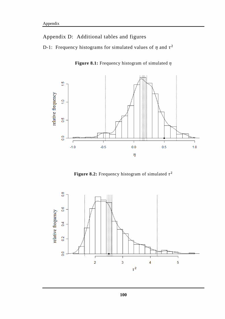
Appendix
100
Appendix D: Additional tables and figures
D-1: Frequency histograms for simulated values of and
Figure 8.1: Frequency histogram of simulated
Figure 8.2: Frequency histogram of simulated

Appendix
101
D-2: Traces of simulated values for Hertig‟s model
Figure 8.3: Traces of simulated , and (Hertig‟s model)
h[2]
iteration
1 5000 10000
0.0
2.0
4.0
6.0
h[3]
iteration
1 5000 10000
0.0
0.25
0.5
0.75
1.0
1.25
h[4]
iteration
1 5000 10000
0.0
0.5
1.0
1.5
h[5]
iteration
1 5000 10000
0.0
0.1
0.2
0.3
0.4
h[6]
iteration
1 5000 10000
0.0
0.2
0.4
0.6
0.8
h[7]
iteration
1 5000 10000
0.0
0.2
0.4
0.6
0.8
h[8]
iteration
1 5000 10000
0.0
0.2
0.4
0.6
h[9]
iteration
1 5000 10000
0.0
2.5
5.0
7.5
10.0
h[10]
iteration
1 5000 10000
0.0
25.0
50.0
75.0
100.0
mu[1]
iteration
1 5000 10000
4.0
6.0
8.0
10.0
mu[2]
iteration
1 5000 10000
-2.0
0.0
2.0
4.0
mu[3]
iteration
1 5000 10000
-0.5
0.0
0.5
1.0
1.5
mu[4]
iteration
1 5000 10000
-0.5
0.0
0.5
1.0
mu[5]
iteration
1 5000 10000
-0.2
0.0
0.2
0.4
0.6
mu[6]
iteration
1 5000 10000
-0.5
0.0
0.5
1.0
mu[7]
iteration
1 5000 10000
-0.5
-0.25
0.0
0.25
0.5
0.75
mu[8]
iteration
1 5000 10000
-0.4
-0.2
0.0
0.2
0.4
mu[9]
iteration
1 5000 10000
-10.0
-5.0
0.0
5.0
10.0
15.0
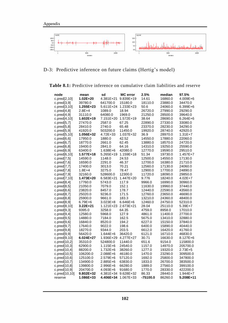
Appendix
102
D-3: Predictive inference on future claims (Hertig‟s model)
Table 8.1: Predictive inference on cumulative claim liabilities and reserve
node mean sd MC error 2.5% median 97.5% c.pred[2,10] 1.02E+20 4.381E+21 9.839E+19 14.61 16860.0 4.009E+6
c.pred[3,9] 39780.0 641700.0 15180.0 18110.0 23880.0 34470.0 c.pred[3,10] 1.255E+23 5.611E+24 1.233E+23 50.6 24060.0 6.399E+6
c.pred[4,8] 2.8E+4 1089.0 18.94 26720.0 27990.0 29290.0 c.pred[4,9] 31110.0 64080.0 1969.0 21250.0 28500.0 39640.0 c.pred[4,10] 1.602E+19 7.151E+20 1.572E+19 38.64 28690.0 6.264E+6
c.pred[5,7] 27470.0 2587.0 67.25 22890.0 27330.0 33080.0 c.pred[5,8] 28410.0 2740.0 65.48 23370.0 28230.0 34290.0 c.pred[5,9] 41920.0 503200.0 11450.0 19920.0 28740.0 42920.0 c.pred[5,10] 1.056E+32 4.72E+33 1.037E+32 36.9 28970.0 1.31E+7
c.pred[6,6] 17950.0 1880.0 42.52 14550.0 17880.0 22060.0 c.pred[6,7] 18770.0 2661.0 62.45 13880.0 18570.0 24720.0 c.pred[6,8] 19400.0 2841.0 64.16 14310.0 19250.0 25590.0 c.pred[6,9] 63400.0 1.638E+6 42080.0 12770.0 19590.0 29510.0 c.pred[6,10] 1.577E+18 5.265E+19 1.159E+18 51.34 19730.0 1.457E+7
c.pred[7,5] 14590.0 1148.0 24.53 12500.0 14550.0 17130.0 c.pred[7,6] 16590.0 2291.0 46.37 12700.0 16380.0 21710.0 c.pred[7,7] 17400.0 3013.0 70.21 12560.0 17130.0 24060.0 c.pred[7,8] 1.8E+4 3275.0 78.47 12900.0 17700.0 24890.0 c.pred[7,9] 32160.0 528600.0 12300.0 11720.0 18090.0 29850.0 c.pred[7,10] 1.473E+20 6.583E+21 1.447E+20 9.776 18240.0 4.02E+7
c.pred[8,4] 17760.0 5743.0 117.9 9966.0 16990.0 30960.0 c.pred[8,5] 21050.0 7079.0 152.1 11630.0 19960.0 37440.0 c.pred[8,6] 23820.0 8457.0 178.7 12440.0 22590.0 43560.0 c.pred[8,7] 25020.0 9236.0 171.5 12760.0 23650.0 46690.0 c.pred[8,8] 25900.0 9661.0 183.3 13210.0 24360.0 48400.0 c.pred[8,9] 6.79E+6 3.023E+8 6.646E+6 12460.0 24750.0 52310.0 c.pred[8,10] 3.22E+21 1.121E+23 2.673E+21 28.04 25110.0 5.39E+7
c.pred[9,3] 9395.0 3258.0 64.35 4759.0 8958.0 17010.0 c.pred[9,4] 12580.0 5968.0 127.9 4861.0 11400.0 27700.0 c.pred[9,5] 14880.0 7184.0 162.5 5675.0 13410.0 32880.0 c.pred[9,6] 16840.0 8520.0 194.2 6227.0 15150.0 37840.0 c.pred[9,7] 17640.0 9022.0 198.6 6400.0 15890.0 40440.0 c.pred[9,8] 18270.0 9344.0 203.5 6612.0 16420.0 41760.0 c.pred[9,9] 56420.0 1.644E+6 36420.0 6121.0 16710.0 46830.0 c.pred[9,10] 6.024E+27 1.936E+29 4.277E+27 30.71 16630.0 8.127E+6
c.pred[10,2] 35310.0 524800.0 11440.0 651.6 9154.0 115800.0 c.pred[10,3] 62900.0 1.115E+6 24540.0 1157.0 14970.0 205700.0 c.pred[10,4] 88200.0 1.732E+6 38260.0 1277.0 19320.0 2.73E+5 c.pred[10,5] 106200.0 2.088E+6 46180.0 1470.0 23290.0 309500.0 c.pred[10,6] 125100.0 2.579E+6 57120.0 1692.0 25800.0 347800.0 c.pred[10,7] 134900.0 2.885E+6 63830.0 1833.0 26700.0 383500.0 c.pred[10,8] 139800.0 2.996E+6 66280.0 1889.0 27560.0 399100.0 c.pred[10,9] 204700.0 4.093E+6 91680.0 1770.0 28330.0 422200.0 c.pred[10,10] 9.802E+32 4.381E+34 9.628E+32 86.33 28440.0 1.944E+7 reserve 1.086E+33 4.406E+34 1.067E+33 -75100.0 86260.0 5.208E+11
mu[10]
iteration
1 5000 10000
-150.0
-100.0
-50.0
0.0
50.0
100.0
sigma2
iteration
1 5000 10000
0.0
5.0
10.0
15.0

Appendix
103
D-4: Traces of simulated values for modified Hertig‟s model
Figure 8.4: Traces of simulated , , , and (modified Hertig‟s model)
D-5: Traces of simulated values for development corr. model
Figure 8.5: Traces of simulated , , , , and (dev. corr. model)
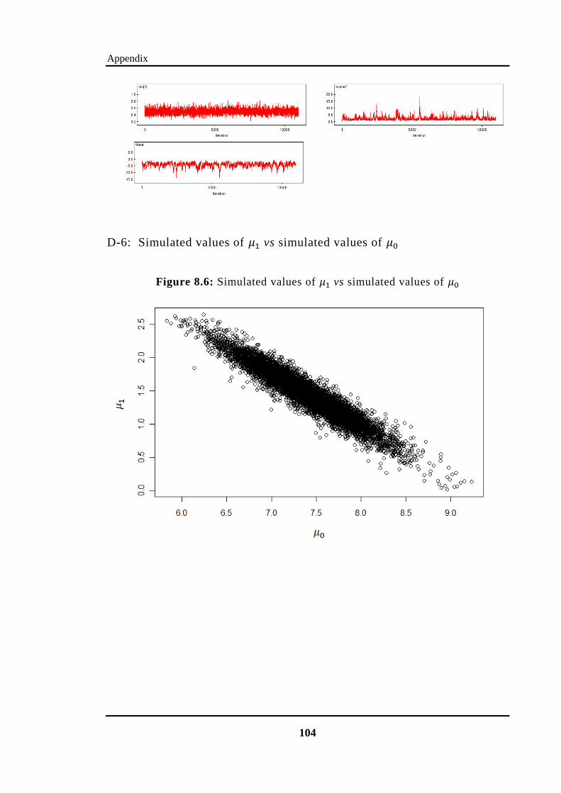
Appendix
104
D-6: Simulated values of vs simulated values of
Figure 8.6: Simulated values of vs simulated values of