bayesian statistical model checking with application to stateflow
TRANSCRIPT

Noname manuscript No.(will be inserted by the editor)
Bayesian Statistical Model Checking with Application toStateflow/Simulink Verification
Paolo Zuliani · Andre Platzer · Edmund M. Clarke
Received: date / Accepted: date
Abstract We address the problem of model checking stochastic systems, i.e., checking
whether a stochastic system satisfies a certain temporal property with a probability
greater (or smaller) than a fixed threshold. In particular, we present a Statistical Model
Checking (SMC) approach based on Bayesian statistics. We show that our approach is
feasible for a certain class of hybrid systems with stochastic transitions, a generaliza-
tion of Simulink/Stateflow models. Standard approaches to stochastic discrete systems
require numerical solutions for large optimization problems and quickly become infea-
sible with larger state spaces. Generalizations of these techniques to hybrid systems
with stochastic effects are even more challenging. The SMC approach was pioneered by
Younes and Simmons in the discrete and non-Bayesian case. It solves the verification
problem by combining randomized sampling of system traces (which is very efficient for
Simulink/Stateflow) with hypothesis testing (i.e., testing against a probability thresh-
old) or estimation (i.e., computing with high probability a value close to the true
probability). We believe SMC is essential for scaling up to large Stateflow/Simulink
models. While the answer to the verification problem is not guaranteed to be correct,
we prove that Bayesian SMC can make the probability of giving a wrong answer arbi-
trarily small. The advantage is that answers can usually be obtained much faster than
with standard, exhaustive model checking techniques. We apply our Bayesian SMC
approach to a representative example of stochastic discrete-time hybrid system mod-
els in Stateflow/Simulink: a fuel control system featuring hybrid behavior and fault
tolerance. We show that our technique enables faster verification than state-of-the-art
statistical techniques. We emphasize that Bayesian SMC is by no means restricted
to Stateflow/Simulink models. It is in principle applicable to a variety of stochastic
models from other domains, e.g., systems biology.
P. ZulianiSchool of Computing Science, Newcastle University, Newcastle, NE1 7RU, UKE-mail: [email protected]
A. Platzer · E. M. ClarkeComputer Science Department, Carnegie Mellon University, Pittsburgh, PA 15213, USAE-mail: aplatzer,[email protected]
2
Keywords Probabilistic verification · Hybrid systems · Stochastic systems · Statistical
model checking · Hypothesis testing · Estimation
1 Introduction
Stochastic effects arise naturally in hybrid systems, for example, because of uncer-
tainties present in the system environment (e.g., the reliability of sensor readings and
actuator effects in control systems, the impact of timing inaccuracies, the reliability of
communication links in a wireless sensor network, or the rate of message arrivals on
an aircraft’s communication bus). Uncertainty can often be modeled via a probabil-
ity distribution, thereby resulting in a stochastic system, i.e., a system which exhibits
probabilistic behavior. This raises the question of how to verify that a stochastic system
satisfies a given probabilistic property. For example, we want to know whether the prob-
ability of an engine controller failing to provide optimal fuel/air ratio is smaller than
0.001; or whether the ignition succeeds within 1ms with probability at least 0.99. In
fact, several temporal logics have been developed in order to express these and other
types of probabilistic properties [3,23,1]. The Probabilistic Model Checking (PMC)
problem is to decide whether a stochastic model satisfies a temporal logic property
with a probability greater than or equal to a certain threshold. More formally, suppose
M is a stochastic model over a set of states S with the starting state s0, φ is a formula
in temporal logic, and θ ∈ (0, 1) is a probability threshold. The PMC problem is to
decide algorithmically whether M |= P≥θ(φ), i.e., to decide whether the model Mstarting from its initial state s0 satisfies the property φ with probability at least θ. In
this paper, property φ is expressed in Bounded Linear Temporal Logic (BLTL), a vari-
ant of LTL [38] in which the temporal operators are equipped with upper time bounds.
Alternatively, BLTL can be viewed as a sublogic of Koymans’ Metric Temporal Logic
[30]. As system models M, we use a stochastic version of hybrid systems modeled in
Stateflow/Simulink.
Existing algorithms for solving the PMC problem fall into one of two categories.
The first category comprises numerical methods that can compute the probability that
the property holds with high precision (e.g., [2,3,11,13,31,22]). Numerical methods
are generally only suitable for finite-state systems of about 107 − 108 states [32]. In
real control systems, the number of states easily exceeds this limit, which motivates
the need for algorithms for solving the PMC problem in a probabilistic fashion, such
as Statistical Model Checking (SMC). These techniques heavily rely on simulation
which, especially for large, complex systems, is generally easier and faster than a full
symbolic study of the system. This can be an important factor for industrial systems
designed using efficient simulation tools like Stateflow/Simulink. Since all we need for
SMC are simulations of the system, we neither have to translate system models into
separate verification tool languages, nor have to build symbolic models of the system
(e.g., Markov chains) appropriate for numerical methods. This simplifies and speeds
up the overall verification process. The most important question, however, is what
information can be concluded from the behavior observed in simulations about the
overall probability that φ holds forM. The key for this are statistical techniques based
on fair (iid = independent and identically distributed) sampling of system behavior.
Statistical Model Checking treats the PMC problem as a statistical inference prob-
lem, and solves it by randomized sampling of the traces (or simulations) from the
model. Each sample trace is model checked to determine whether the BLTL property

3
φ holds, and the number of satisfying traces that are found by randomized sampling
is used to decide whether M |= P≥θ(φ). This decision is made by means of either
estimation or hypothesis testing. In the first case one seeks to estimate probabilistically
(i.e., compute with high probability a value close to) the probability that the prop-
erty holds and then compare that estimate to θ [25,41] (in statistics such estimates are
known as confidence intervals). In the second case, the PMC problem is directly treated
as a hypothesis testing problem [49,41,29], i.e., deciding between the null hypothesis
H0 : M |= P≥θ(φ) (M satisfies φ with probability greater than or equal to θ) versus
the alternative hypothesis H1 :M |= P<θ(φ) (M satisfies φ with probability less than
θ).
The algorithm for SMC by Bayesian hypothesis testing [29] (see Algorithm 1) is
very simple but powerful. It is based exclusively on numerical simulations (called traces)
of the system M to determine whether it accepts H0 or H1.
Input : PBLTL property P>θ(φ), acceptance threshold T > 1, prior density g
for (unknown) probability p that the system satisfies φ
Output: “H0 : p > θ accepted”, or “H1 : p < θ accepted”
1 n := 0; number of traces drawn so far2 x := 0; number of traces satisfying φ so far3 loop
4 σ := draw a sample trace of the system (iid); Section 25 n := n+ 1;
6 if σ |= φ then Section 37 x := x+ 1
8 end
9 B := BayesFactor(n, x); Section 510 if (B > T ) then return “H0 accepted”;
11 if (B < 1T ) then return “H1 accepted”
12 end loop;
Algorithm 1: Statistical Model Checking by Bayesian Hypothesis Testing
The SMC algorithm repeatedly simulates the system to draw sample traces from
the system model M (line 4). For each sample trace σ, SMC checks whether or not σ
satisfies the BLTL property φ (line 6) and increments the number of successes (x in
line 7). At this point, the algorithm uses a statistical test, the Bayes factor test (line 9),
to choose one of three things to do. The algorithm determines that it has seen enough
data and accepts H0 (line 10), or it determines that it has seen enough to accept the
alternative hypothesis H1 (line 11), or it decides that it has not yet seen statistically
conclusive evidence and needs to repeat drawing sample traces (when 1T ≤ B ≤ T ).
The value of the Bayes factor B gets larger when we see more statistical evidence in
favor of H0. It gets smaller when we see more statistical evidence in favor of H1. If
B exceeds a user-specified threshold T , the SMC algorithm accepts hypothesis H0. If
B becomes smaller than 1T , the SMC algorithm rejects H0 and accepts H1 instead.
Otherwise B is inconclusive and the SMC algorithm repeats.
Algorithm 1 is very simple and generic. In order to be able to use it, we do, however,
need to provide system models, a way of sampling from them efficiently, and a way
to check properties for a given trace. In particular, for line 4, SMC needs a class of
system models that is suitable for the application domain along with a way to sample
traces from the system model. For correctness, it is imperative that the sample traces

4
be drawn from the model in a fair (iid) way and that the resulting probabilities are
well-defined. We investigate these questions in Section 2. For line 6, SMC needs a
way to check a BLTL property along a given trace σ of the system. We investigate
how this can be done and why it is well-defined for simulations, which can only have
finite length, in Section 3. For line 9, we need an efficient way to compute the statistic
employed, i.e., the Bayes factor — this is developed in Section 5.
Note that Statistical Model Checking cannot guarantee a correct answer of the
PMC problem. The most crucial question needed to obtain meaningful results from
SMC is whether the probability that the algorithm gives a wrong answer can be
bounded. In Section 6 we prove that this error probability can indeed be bounded
arbitrarily by the user. In Section 4, we also introduce a new form of SMC that uses
Bayesian estimation instead of Bayesian hypothesis testing. Hypothesis-testing based
methods are more efficient than those based on estimation when the threshold probabil-
ity θ (which is specified by the user) is significantly different from the true probability
that the property holds (which is determined by M and its initial state s0) [48]. In
this paper we show that our Bayesian estimation algorithm can be very efficient for
probabilities close to 1 or close to 0.
Our SMC approach thus encompasses both hypothesis testing and estimation, and
it is based on Bayes’ theorem and sequential sampling. Bayes’ theorem enables us to in-
corporate prior information about the model being verified. Sequential sampling means
that the number of sampled traces is not fixed a priori. Instead, sequential algorithms
determine the sample size at “run-time”, depending on the evidence gathered by the
samples seen so far. Because conclusive information from the samples can be used to
stop our SMC algorithms as early as possible, this often leads to significantly smaller
number of sampled traces (simulations).
We apply our approach to a representative example of discrete-time stochastic
hybrid systems modeled in Stateflow/Simulink: a fault-tolerant fuel control system.
The contributions of this paper are as follows:
– We show how Statistical Model Checking can be used for Stateflow/Simulink-style
hybrid systems with probabilistic transitions.
– We introduce Bayesian sequential interval estimation and prove almost sure termi-
nation.
– We prove analytic error bounds for the Bayesian sequential hypothesis testing and
estimation algorithms.
– In a series of experiments with a relevant Stateflow/Simulink model, we empirically
show that our sequential estimation method performs better than other estimation-
based Statistical Model Checking approaches. In some cases our algorithm is faster
by several orders of magnitudes.
While the theoretical analysis of our Statistical Model Checking approach is compli-
cated by its sequential nature, a beneficial property of our algorithms is that they
are easy to implement and often more efficient than working with a fixed number of
samples.
2 Model
Our Statistical Model Checking algorithms can be applied to any stochastic model for
which it is possible to define a probability space over its traces, draw sample traces

5
in a fair way, and check BLTL properties for traces. Several stochastic models like
discrete/continuous Markov chains satisfy this property [50]. Here we use discrete-time
hybrid systems a la Stateflow/Simulink with probabilistic transitions.
Stateflow/Simulink1 (SF/SL) is a model-based design and simulation tool devel-
oped by The Mathworks. It provides a graphical environment for designing data-flow
programming architectures. It is heavily used in the automotive and defense indus-
tries for developing embedded systems. Models in SF/SL are recursively defined by
blocks, which may contain specifications (in fact, blocks themselves) of communication,
control, signal processing, and of many other types of computation. The blocks of a
model are interconnected by signals. In Simulink, blocks operate with a continuous-
time semantics, which means that the model’s signals are thought to be continuous-
time functions. (For example, the output of an integrator block is a continuous-time
signal.) Stateflow introduces discrete-time computations in the form of discrete-time
finite-state automata which can be freely embedded in Simulink blocks. The resulting
models have thus a hybrid continuous/discrete-time semantics. The model simulation
is accomplished by a solver (a numerical integration procedure) which calculates the
temporal dynamics of the model. Finally, SF/SL provides for automated code gener-
ation (e.g., C) from the models. This feature is used when the model is ready to be
deployed on the target hardware architecture.
Preliminaries We consider discrete-time stochastic processes over Rn. Given a Borel
set S ⊆ Rn, we denote its Borel σ-algebra by B(S). We use the notion of stochas-
tic kernel as a unifying concept for our particular model of stochastic hybrid system.
Note that, unlike other models of stochastic hybrid systems [18,6,8,35,37], we do not
consider continuous stochastic transitions, since those are less relevant for SF/SL ap-
plications.
Definition 1 A stochastic kernel on a measurable space (S,B(S)) is a function K:S×B(S)→ [0, 1] such that:
1. for each x ∈ S, K(x, ·) is a probability measure on B(S); and
2. for each B ∈ B(S), K(·, B) is a (Borel) measurable function on S.
The sample space is the set Ω = Sω of (infinite) sequences of states, equipped with
the usual product σ-algebra F of Ω (i.e., F is the smallest σ-algebra containing all the
cylinder sets over B(Sn), for all n > 1.) Given a stochastic kernel K on (Ω,F) and an
initial state x ∈ S, by Ionescu Tulcea’s theorem [43, Theorem 2 in II.9] there exists a
unique probability measure P defined on (Ω,F) and a Markov process Xt : t ∈ Nsuch that for all B ∈ B(S) and for all xi ∈ S:
– P(X1 ∈ B) = δx(B); and
– P(Xt+1 ∈ B | (x1, . . . , xt)) = P(Xt+1 ∈ B |xt) = K(xt, B)
where δx is the Dirac measure (i.e., δx(B) = 1 if x ∈ B, and 0 otherwise). Observe
that we can formally assume all samples to be infinitely long by adding stuttering
transitions for executions that have terminated.
1 http://www.mathworks.com/products/simulink/

6
Discrete-Time Hybrid Systems As a system model, we consider discrete-time hy-
brid systems with additional probabilistic transitions (our case study uses SF/SL).
Such a model gives rise to a transition system that allows for discrete transitions (e.g.,
from one Stateflow node to another), continuous transitions (when following differen-
tial equations underlying Simulink models), and probabilistic transitions (following a
known probability distribution modeled in SF/SL). For SF/SL, a state assigns real val-
ues to all the state variables and identifies the current location for Stateflow machines.
We first define a deterministic hybrid automaton. Then we augment it with prob-
abilistic transitions.
Definition 2 A discrete-time hybrid automaton (DTHA) consists of:
– a continuous state space Rn;
– a directed graph with vertices Q (locations) and edges E (control switches);
– one initial state (q0, x0) ∈ Q× Rn;
– continuous flows ϕq(t;x) ∈ Rn, representing the (continuous) state reached after
staying in location q for time t ≥ 0, starting from x ∈ Rn;
– jump functions jumpe : Rn → Rn for edges e ∈ E.
Definition 3 The transition function for a deterministic DTHA is defined over Q×Rn
as
(q, x)→∆(q,x) (q, x)
where
– for t ∈ R≥0, we have (q, x)→t (q, x) iff x = ϕq(t;x);
– for e ∈ E, we have (q, x)→e (q, x) iff x = jumpe(x) and e is an edge from q to q;
– ∆ : Q× Rn → R≥0 ∪ E is the simulation function.
The simulation function ∆ makes system runs deterministic by selecting which par-
ticular discrete or continuous transition to execute from the current state. For State-
flow/Simulink, ∆ satisfies several properties, including that the first edge that is en-
abled (i.e., where a jump is possible) will be chosen. Furthermore, if an edge is enabled,
a discrete transition will be taken rather than a continuous transition. We note that
Stateflow/Simulink’s default ordering of outgoing edges is by clockwise orientation in
the graphical notation, but allows user-specified precedence overrides as well.
Each execution of a DTHA is obtained by following the transition function re-
peatedly from state to state. A sequence σ = (s0, t0), (s1, t1), . . . of si ∈ Q × Rn and
ti ∈ R≥0 is called trace iff, s0 = (q0, x0) and for each i ∈ N, si →∆(si) si+1 and:
1. ti = ∆(si) if ∆(si) ∈ R≥0 (continuous transition), or
2. ti = 0 if ∆(si) ∈ E (discrete transition).
Thus the system follows transitions from si to si+1. If this transition is a continuous
transition, then ti is its duration ∆(si), otherwise ti = 0 for discrete transitions. In
particular, the global time at state si = (qi, xi) isP
0≤l<i tl. We require that the sumP∞i ti must diverge, that is, the system cannot make infinitely many state switches in
finite time (non-zeno).
7
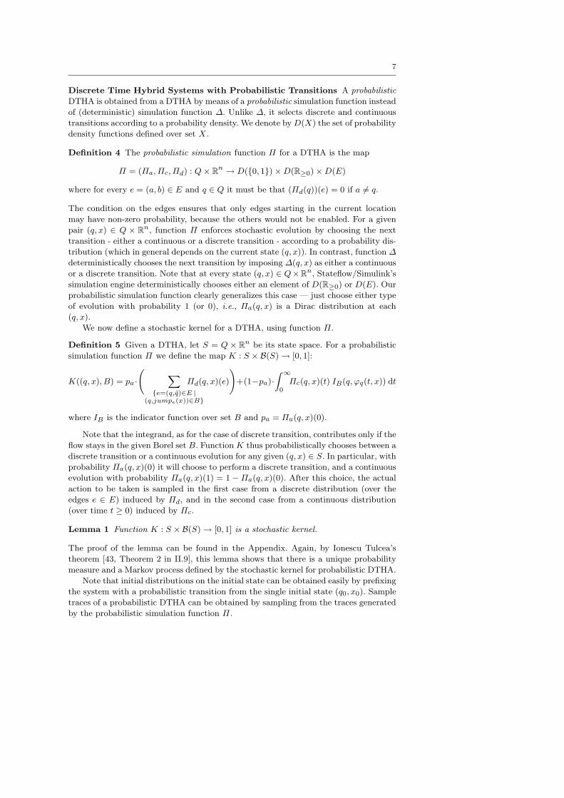
Discrete Time Hybrid Systems with Probabilistic Transitions A probabilistic
DTHA is obtained from a DTHA by means of a probabilistic simulation function instead
of (deterministic) simulation function ∆. Unlike ∆, it selects discrete and continuous
transitions according to a probability density. We denote by D(X) the set of probability
density functions defined over set X.
Definition 4 The probabilistic simulation function Π for a DTHA is the map
Π = (Πa, Πc, Πd) : Q× Rn → D(0, 1)×D(R≥0)×D(E)
where for every e = (a, b) ∈ E and q ∈ Q it must be that (Πd(q))(e) = 0 if a 6= q.
The condition on the edges ensures that only edges starting in the current location
may have non-zero probability, because the others would not be enabled. For a given
pair (q, x) ∈ Q × Rn, function Π enforces stochastic evolution by choosing the next
transition - either a continuous or a discrete transition - according to a probability dis-
tribution (which in general depends on the current state (q, x)). In contrast, function ∆
deterministically chooses the next transition by imposing ∆(q, x) as either a continuous
or a discrete transition. Note that at every state (q, x) ∈ Q×Rn, Stateflow/Simulink’s
simulation engine deterministically chooses either an element of D(R≥0) or D(E). Our
probabilistic simulation function clearly generalizes this case — just choose either type
of evolution with probability 1 (or 0), i.e., Πa(q, x) is a Dirac distribution at each
(q, x).
We now define a stochastic kernel for a DTHA, using function Π.
Definition 5 Given a DTHA, let S = Q × Rn be its state space. For a probabilistic
simulation function Π we define the map K : S × B(S)→ [0, 1]:
K((q, x), B) = pa ·
Xe=(q,q)∈E |
(q,jumpe(x))∈B
Πd(q, x)(e)
!+(1−pa)·
Z ∞0Πc(q, x)(t) IB(q, ϕq(t, x)) dt
where IB is the indicator function over set B and pa = Πa(q, x)(0).
Note that the integrand, as for the case of discrete transition, contributes only if the
flow stays in the given Borel set B. Function K thus probabilistically chooses between a
discrete transition or a continuous evolution for any given (q, x) ∈ S. In particular, with
probability Πa(q, x)(0) it will choose to perform a discrete transition, and a continuous
evolution with probability Πa(q, x)(1) = 1−Πa(q, x)(0). After this choice, the actual
action to be taken is sampled in the first case from a discrete distribution (over the
edges e ∈ E) induced by Πd, and in the second case from a continuous distribution
(over time t ≥ 0) induced by Πc.
Lemma 1 Function K : S × B(S)→ [0, 1] is a stochastic kernel.
The proof of the lemma can be found in the Appendix. Again, by Ionescu Tulcea’s
theorem [43, Theorem 2 in II.9], this lemma shows that there is a unique probability
measure and a Markov process defined by the stochastic kernel for probabilistic DTHA.
Note that initial distributions on the initial state can be obtained easily by prefixing
the system with a probabilistic transition from the single initial state (q0, x0). Sample
traces of a probabilistic DTHA can be obtained by sampling from the traces generated
by the probabilistic simulation function Π.

8
Embedding Stateflow/Simulink SF/SL is a very sophisticated tool for embedded
system design and simulation, and it is very challenging to define a comprehensive
semantics for it. See the work of Tiwari [44] for a remarkable effort to define a formal
semantics. Since Statistical Model Checking is based on numerical simulation, we do not
need to know a full formal semantics of Stateflow/Simulink here. We can simply use its
simulation engine (solver) to generate traces. What we assume, however, is that State-
flow/Simulink is well-behaved in terms of defining a probabilistic simulation function
Π. Basically, Simulink primarily drives the continuous transitions (computed by numer-
ical integration schemes) and interfaces with Stateflow blocks that determine the transi-
tion guards and discrete jumps. The continuous state space of the corresponding DTHA
is some subset of Rn where n is the number of variables in the Stateflow/Simulink
model. The locations Q and edges E correspond to the discrete transitions found in
Stateflow/Simulink, also see [44]. For every state (q, x) ∈ S, Simulink/Stateflow, in
fact, chooses deterministically whether a discrete transition (Πa(q, x)(0)) or a continu-
ous transition (Πa(q, x)(1)) is performed next. That is, Πa(q, x) is deterministic. The
discrete transition Πd(q, x) is also, for the most part, chosen deterministically based
on the block placement or precedence numbers for enabled transitions. Randomness
enters, however, in the outcome of random blocks introduced in the design by the user.
The durations of continuous transitions are determined by the Simulink integration
engine in a nontrivial way. What matters for us is not what exactly the distributions
are that Stateflow/Simulink chooses for Πa, Πc, Πd. Statistical model checking does
not need whitebox access to the system model. It only needs a way to draw iid sample
traces (cf. line 4 in Algorithm 1). What does matter, however, for Statistical Model
Checking to work is the assumption that there is a well-defined probability measure
over the trace space.
3 Specifying Properties in Temporal Logic
Our algorithm verifies properties expressed as Probabilistic Bounded Linear Temporal
Logic (PBLTL) formulas. We first define the syntax and semantics of (non-probabilistic)
Bounded Linear Temporal Logic (BLTL), which we can check on a single trace, and
then extend that logic to PBLTL. Finkbeiner and Sipma [16] have defined a variant of
LTL on finite traces of discrete-event systems (where time is thus not considered).
For a stochastic model M, let the set of state variables SV be a finite set of real-
valued variables. A Boolean predicate over SV is a constraint of the form y∼v, where
y ∈ SV , ∼ ∈ ≥,≤,=, and v ∈ R. A BLTL property is built on a finite set of Boolean
predicates over SV using Boolean connectives and temporal operators. The syntax of
the logic is given by the following grammar:
φ ::= y∼v | (φ1 ∨ φ2) | (φ1 ∧ φ2) | ¬φ1 | (φ1Utφ2),
where ∼ ∈ ≥,≤,=, y ∈ SV , v ∈ Q, and t ∈ Q≥0. As usual, we can define additional
temporal operators such as the operator “eventually within time t” which is defined
as Ftψ = True Ut ψ, or the operator “always up to time t”, which is defined as
Gtψ = ¬Ft¬ψ.
We define the semantics of BLTL with respect to (infinite) executions of the model
M. The fact that an execution σ satisfies property φ is denoted by σ |= φ. We denote
the trace suffix starting at step i by σi (in particular, σ0 denotes the original trace σ).
We denote the value of the state variable y in σ at step i by V (σ, i, y).

9
Definition 6 The semantics of BLTL for a trace σk starting at the kth state (k ∈ N)
is defined as follows:
– σk |= y ∼ v if and only if V (σ, k, y) ∼ v;
– σk |= φ1 ∨ φ2 if and only if σk |= φ1 or σk |= φ2;
– σk |= φ1 ∧ φ2 if and only if σk |= φ1 and σk |= φ2;
– σk |= ¬φ1 if and only if σk |= φ1 does not hold (written σk 6|= φ1);
– σk |= φ1Utφ2 if and only if there exists i ∈ N such that
(a)X
0≤l<itk+l ≤ t,
(b) σk+i |= φ2, and
(c) σk+j |= φ1 for each 0 ≤ j < i.
Statistical Model Checking decides the probabilistic Model Checking problem by re-
peatedly checking whether σ |= φ holds on sample simulations σ of the system. In
practice, sample simulations only have a finite duration. The question is how long
these simulations have to be for the formula φ to have a well-defined semantics such
that σ |= φ can be checked (line 6 of Algorithm 1 on p. 3). If σ is too short, say of
duration 2, the semantics of φ1U5.3φ2 may be unclear if φ2 is false for duration 2. But
at what duration of the simulation can we stop because we know that the truth-value
for σ |= φ will never change by continuing the simulation? Is the number of required
simulation steps expected to be finite at all?
For a class of finite length continuous-time boolean signals, well-definedness of
checking bounded MITL properties has been conjectured in [34]. Here we generalize
to infinite, hybrid traces with real-valued signals. We prove well-definedness and the
fact that a finite prefix of the discrete time hybrid signal is sufficient for BLTL model
checking, which is crucial for termination.
Lemma 2 (Bounded sampling) The problem “σ |= φ” is well-defined and can be
checked for BLTL formulas φ and traces σ based on only a finite prefix of σ of bounded
duration.
For proving Lemma 2 we need to derive bounds on when to stop simulation. Those
time bounds can be read off easily from the BLTL formula:
Definition 7 [34] The sampling bound #(φ) ∈ Q≥0 of a BLTL formula φ is the
maximum nested sum of time bounds:
#(y ∼ v) := 0
#(¬φ1) := #(φ1)
#(φ1 ∨ φ2) := max(#(φ1),#(φ2))
#(φ1 ∧ φ2) := max(#(φ1),#(φ2))
#(φ1Utφ2) := t+ max(#(φ1),#(φ2))
The next lemma (proof in the Appendix) shows that the semantics of BLTL formulas
φ is well-defined on finite prefixes of traces with a duration that is bounded by #(φ).
Lemma 3 (BLTL on bounded simulation traces) Let φ be a BLTL formula, k ∈N. Then for any two infinite traces σ = (s0, t0), (s1, t1), . . . and σ = (s0, t0), (s1, t1), . . .
with
sk+I = sk+I and tk+I = tk+I ∀I ∈ N withX
0≤l<Itk+l ≤ #(φ) (1)
we have that
σk |= φ iff σk |= φ .

10
As a consequence, for checking σ |= φ during the Statistical Model Checking al-
gorithm 1, we can stop simulation of the sample σ when the duration exceeds #(φ),
because, according to Lemma 3, all possible extensions of the trace agree on whether
φ holds or not. In the Appendix we prove that Lemma 2 holds using prefixes of traces
according to the sampling bound #(φ), which guarantees that finite simulations are
sufficient for deciding whether φ holds on a trace. Note that #(φ) is not the maximal
number of transitions until formula φ can be decided along a trace, but only an upper
bound for the amount of time that passes in the model M until φ can be decided.
In particular, divergence of time on samples is required to ensure that the number of
transitions is finite as well and that SMC terminates. Observe that ad-hoc ways of
ensuring divergence of time by discarding samples with too slow a progress of time
may bias the outcome of SMC.
We now define Probabilistic Bounded Linear Temporal Logic.
Definition 8 A Probabilistic Bounded LTL (PBLTL) formula is a formula of the form
P≥θ(φ), where φ is a BLTL formula and θ ∈ (0, 1) is a probability.
We say thatM satisfies PBLTL property P≥θ(φ), denoted byM |= P≥θ(φ), if and only
if the probability that an execution trace ofM satisfies BLTL property φ is greater than
or equal to θ. This problem is well-defined, since by Lemma 2, each σ |= φ is decidable
on a finite prefix of σ, and in the previous Section we have proved existence of a
probability measure over the traces ofM. Thus, the set of all (non-zeno) executions of
M that satisfy a given BLTL formula is measurable [50]. Note that counterexamples to
the BLTL property φ are not counterexamples to the PBLTL property P≥θ(φ), because
the truth of P≥θ(φ) depends on the likelihood of all counterexamples to φ. This makes
PMC more difficult than standard Model Checking, because one counterexample to φ
is not enough to decide P≥θ(φ). We refer to the excellent overview [9] for a discussion
of counterexamples in Probabilistic Model Checking.
4 Bayesian Interval Estimation
We present our new Bayesian statistical estimation algorithm. In this approach we are
interested in estimating p, the (unknown) probability that a random execution trace of
M satisfies a fixed BLTL property φ. The estimate will be in the form of a confidence
interval, i.e., an interval which will contain p with arbitrarily high probability.
For any trace σi of the systemM, we can, according to Lemma 2, deterministically
decide whether σi satisfies BLTL formula φ. Therefore, we can define a Bernoulli ran-
dom variable Xi denoting the outcome of σi |= φ. The conditional probability density
function associated with Xi is thus:
f(xi|u) = uxi(1− u)1−xi (2)
where xi = 1 iff σi |= φ, otherwise xi = 0. Note that the Xi are (conditionally)
independent and identically distributed (iid) random variables, as each trace is given
by an independent execution of the model. Since p (the probability that property φ
holds) is unknown, in the Bayesian approach one assumes that p is given by a random
variable, whose density g(·) is called the prior density. The prior is usually based on
our previous experiences and beliefs about the system. A lack of information about
11
the probability of the system satisfying the formula is usually summarized by a non-
informative or objective prior (see [39, Section 3.5] for an in-depth treatment).
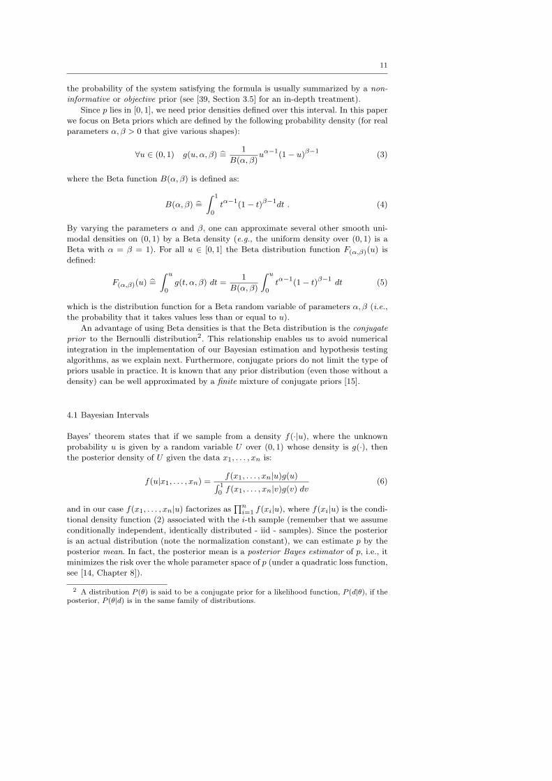
Since p lies in [0, 1], we need prior densities defined over this interval. In this paper
we focus on Beta priors which are defined by the following probability density (for real
parameters α, β > 0 that give various shapes):
∀u ∈ (0, 1) g(u, α, β) b= 1
B(α, β)uα−1(1− u)β−1 (3)
where the Beta function B(α, β) is defined as:
B(α, β) b= Z 1
0tα−1(1− t)β−1dt . (4)
By varying the parameters α and β, one can approximate several other smooth uni-
modal densities on (0, 1) by a Beta density (e.g., the uniform density over (0, 1) is a
Beta with α = β = 1). For all u ∈ [0, 1] the Beta distribution function F(α,β)(u) is
defined:
F(α,β)(u) b= Z u
0g(t, α, β) dt =
1
B(α, β)
Z u
0tα−1(1− t)β−1 dt (5)
which is the distribution function for a Beta random variable of parameters α, β (i.e.,
the probability that it takes values less than or equal to u).
An advantage of using Beta densities is that the Beta distribution is the conjugate
prior to the Bernoulli distribution2. This relationship enables us to avoid numerical
integration in the implementation of our Bayesian estimation and hypothesis testing
algorithms, as we explain next. Furthermore, conjugate priors do not limit the type of
priors usable in practice. It is known that any prior distribution (even those without a
density) can be well approximated by a finite mixture of conjugate priors [15].
4.1 Bayesian Intervals
Bayes’ theorem states that if we sample from a density f(·|u), where the unknown
probability u is given by a random variable U over (0, 1) whose density is g(·), then
the posterior density of U given the data x1, . . . , xn is:
f(u|x1, . . . , xn) =f(x1, . . . , xn|u)g(u)R 1
0 f(x1, . . . , xn|v)g(v) dv(6)
and in our case f(x1, . . . , xn|u) factorizes asQni=1 f(xi|u), where f(xi|u) is the condi-
tional density function (2) associated with the i-th sample (remember that we assume
conditionally independent, identically distributed - iid - samples). Since the posterior
is an actual distribution (note the normalization constant), we can estimate p by the
posterior mean. In fact, the posterior mean is a posterior Bayes estimator of p, i.e., it
minimizes the risk over the whole parameter space of p (under a quadratic loss function,
see [14, Chapter 8]).
2 A distribution P (θ) is said to be a conjugate prior for a likelihood function, P (d|θ), if theposterior, P (θ|d) is in the same family of distributions.

12
For a coverage goal c ∈ ( 12 , 1), any interval (t0, t1) such thatZ t1
t0
f(u|x1, . . . , xn) du = c (7)
is called a 100c percent Bayesian interval estimate of p. Naturally, one would choose
t0 and t1 that minimize t1 − t0 and satisfy (7), thus determining an optimal interval.
(Note that t0 and t1 are in fact functions of the sample x1, . . . , xn.) Optimal interval
estimates can be found, for example, for the mean of a normal distribution with normal
prior, where the resulting posterior is normal. In general, however, it is difficult to find
optimal interval estimates. For unimodal posterior densities like Beta densities, we can
use the posterior’s mean as the “center” of an interval estimate.
Here, we do not pursue the computation of an optimal interval, which may be
numerically infeasible. Instead, we fix a desired half-interval width δ and then sample
until the posterior probability of an interval of width 2δ containing the posterior mean
exceeds c. When sampling from a Bernoulli distribution and with a Beta prior of
parameters α, β, it is known that the mean p of the posterior is:
p =x+ α
n+ α+ β(8)
where x =Pni=1 xi is the number of successes in the sampled data x1, . . . , xn. The
integral in (7) can be computed easily in terms of the Beta distribution function.
Proposition 1 Let (t0, t1) be an interval in [0, 1]. The posterior probability of Bernoulli
iid samples (x1, . . . , xn) and Beta prior of parameters α, β > 0 can be calculated as:Z t1
t0
f(u|x1, . . . , xn) du = F(x+α,n−x+β)(t1)− F(x+α,n−x+β)(t0) (9)
where x =Pni=1 xi is the number of successes in (x1, . . . , xn) and F (·) is the Beta
distribution function.
Proof Direct from definition of Beta distribution function (5) and the fact that the
posterior density is a Beta of parameters x+ α and n− x+ β. ut
The Beta distribution function can be computed with high accuracy by standard math-
ematical libraries (e.g. the GNU Scientific Library) or software (e.g. Matlab). Hence,
as also argued in the previous section, the Beta distribution is the appropriate choice
for summarizing the prior distribution in Statistical Model Checking.
4.2 Bayesian Estimation Algorithm
We want to compute an interval estimate of p = Prob(M |= φ), where φ is a BLTL
formula and M a stochastic hybrid system model - remember from our discussion in
Sections 2 and 3 that p is well-defined (but unknown). Fix the half-size δ ∈ (0, 12 ) of
the desired interval estimate for p, the interval coverage coefficient c ∈ ( 12 , 1) to be
used in (7), and the coefficients α, β of the Beta prior.
Our algorithm (shown in Algorithm 2) iteratively draws iid sample traces σ1, σ2, . . .,
and checks whether they satisfy φ. At stage n, the algorithm computes the posterior

13
mean p, which is the Bayes estimator for p, according to (8). Next, using t0 = p − δ,t1 = p+ δ it computes the posterior probability of the interval (t0, t1) as
γ =
Z t1
t0
f(u|x1, . . . , xn) du .
Input : BLTL Property φ, half-interval size δ ∈ (0, 12 ), interval coverage
coefficient c ∈ ( 12 , 1), Prior Beta distribution with parameters α, β for
the (unknown) probability p that the system satisfies φ
Output: An interval (t0, t1) of width 2δ with posterior probability at least c,
estimate p for the true probability p
1 n := 0; number of traces drawn so far2 x := 0; number of traces satisfying φ so far3 repeat
4 σ := draw a sample trace of the system (iid);
5 n := n+ 1;
6 if σ |= φ then x := x+ 1;
7 p := (x+ α)/(n+ α+ β); compute posterior mean8 (t0, t1) := (p− δ, p+ δ); compute interval estimate9 if t1 > 1 then (t0, t1) := (1− 2 · δ, 1)
10 else if t0 < 0 then (t0, t1) := (0, 2 · δ);compute posterior probability of p ∈ (t0, t1), by (9)
11 γ := PosteriorProb(t0, t1)
12 until (γ > c);
13 return (t0, t1), p
Algorithm 2: Statistical Model Checking by Bayesian Interval Estimates
If γ > c the algorithm stops and returns t0, t1 and p; otherwise it samples another
trace and repeats. One should pay attention at the extreme points of the (0, 1) interval,
but those are easily taken care of, as shown in lines 9 and 10 of Algorithm 2. Note that
the algorithm always returns an interval of width 2δ.
In Figure 1 we give three snapshots of a typical execution of the algorithm. We
have plotted the posterior density (6) after 1000 and 5000 samples, and on termination
of the algorithm (which occurred after 14775 samples for this specific run.) In this
experiment, we have replaced system simulation and trace checking by tossing a coin
with a fixed bias. Therefore, the Bayesian estimation algorithm will compute both
interval and point estimates for such (unknown) bias. The true coin bias (i.e., the
probability of success) used was 0.84, while half-interval size was δ = 0.01, coverage
probability was c = 0.999, and the prior was uniform (α = β = 1). From Figure 1
we can see that after 1000 samples the posterior density is almost entirely within the
[0.825, 0.9] interval. However, as the algorithm progresses to 5000 samples, the posterior
density gets “leaner” and “taller”, i.e., its mass is concentrated over a shorter interval,
thereby giving better (tighter) estimates. On termination, after 14775 samples for this
run, the posterior density becomes even more thin, and satisfies the required coverage
probability (c) and half-interval size (δ) specified by the user.
Finally, we note that the posterior mean p is a biased estimator of the true proba-
bility p — the expected value of p is not p, as it can be easily seen from p’s definition
(8). However, this is not a problem, since unbiasedness is a rather weak property of
estimators for the mean. (Unbiased estimators are easy to get: from a sample of iid

14
0.65 0.7 0.75 0.8 0.85 0.90
20
40
60
80
100
120
140
At n = 1000 samples (x = 860 successes)At n = 5000 samples (x = 4232 successes)On termination (n = 14775, x = 12370)
Fig. 1 Posterior density for sequential Bayesian estimation (Algorithm 2) at several samplesizes; the unknown probability is 0.84, δ = 0.01, c = 0.999, uniform prior (α = β = 1). Forreadability the graph is restriced to [0.65, 0.9].
variables estimate their mean by using any one sample. This estimator is unbiased
by definition, but of course not useful.) More importantly, the posterior mean p is a
consistent estimator, i.e., it converges in probability to p as the sample size tends to
infinity (this is immediate from (8) and the Law of Large Numbers.) Therefore, larger
sample sizes will generally yields more accurate estimates, as it is witnessed by Figure
1, and as one would expect from a “good” estimator. We remark that the consistency
of p is independent from the choice of the prior.
5 Bayesian Hypothesis Testing
In this section we briefly present the sequential Bayesian hypothesis test, which was
introduced in [29]. Recall that the PMC problem is to decide whether M |= P≥θ(φ),
where θ ∈ (0, 1) and φ is a BLTL formula. Let p be the (unknown but fixed) probability
of the model satisfying φ: thus, the PMC problem can now be stated as deciding
between two hypotheses:
H0 : p > θ H1 : p < θ. (10)
Let X1, . . . , Xn be a sequence of Bernoulli random variables defined as for the PMC
problem in Sect. 4, and let d = (x1, . . . , xn) denote a sample of those variables. Let H0
and H1 be mutually exclusive hypotheses over the random variable’s parameter space
according to (10). Suppose the prior probabilities P (H0) and P (H1) are strictly positive
and satisfy P (H0) + P (H1) = 1. Bayes’ theorem states that the posterior probabilities

15
are:
P (Hi|d) =P (d|Hi)P (Hi)
P (d)(i = 0, 1) (11)
for every d with P (d) = P (d|H0)P (H0) + P (d|H1)P (H1) > 0. In our case P (d) is
always non-zero (there are no impossible finite sequences of outcomes).
5.1 Bayes Factor
By Bayes’ theorem, the posterior odds for hypothesis H0 is
P (H0|d)
P (H1|d)=P (d|H0)
P (d|H1)· P (H0)
P (H1). (12)
Definition 9 The Bayes factor B of sample d and hypotheses H0 and H1 is
B =P (d|H0)
P (d|H1).
For fixed priors in a given example, the Bayes factor is directly proportional to the
posterior odds by (12). Thus, it may be used as a measure of relative confidence in H0
vs. H1, as proposed by Jeffreys [28]. To test H0 vs. H1, we compute the Bayes factor
B of the available data d and then compare it against a fixed threshold T > 1: we shall
accept H0 iff B > T . Jeffreys interprets the value of the Bayes factor as a measure of
the evidence in favor of H0 (dually, 1B is the evidence in favor of H1). Classically, a fixed
number of samples was suggested for deciding H0 vs. H1. We develop an algorithm
that chooses the number of samples adaptively.
We now show how to compute the Bayes factor. According to Definition 9, we
have to calculate the ratio of the probabilities of the observed sample d = (x1, . . . , xn)
given H0 and H1. By (12), this ratio is proportional to the ratio of the posterior
probabilities, which can be computed from Bayes’ theorem (6) by integrating the joint
density f(x1|·) · · · f(xn|·) with respect to the prior g(·):
P (H0|x1, . . . , xn)
P (H1|x1, . . . , xn)=
R 1θ f(x1|u) · · · f(xn|u) · g(u) duR θ0 f(x1|u) · · · f(xn|u) · g(u) du
.
Thus, the Bayes factor is:
B =π1
π0·R 1θ f(x1|u) · · · f(xn|u) · g(u) duR θ0 f(x1|u) · · · f(xn|u) · g(u) du
(13)
where π0 = P (H0) =R 1θ g(u) du, and π1 = P (H1) = 1−π0. We observe that the Bayes
factor depends on the data d and on the prior g, so it may be considered a measure of
confidence in H0 vs. H1 provided by the data x1, . . . , xn, and “weighted” by the prior
g. When using Beta priors, the calculation of the Bayes factor can be much simplified.

16
Proposition 2 The Bayes factor of H0 : p > θ vs. H1 : p < θ with Bernoulli samples
(x1, . . . , xn) and Beta prior of parameters α, β is:
Bn =π1
π0·
1
F(x+α,n−x+β)(θ)− 1
!.
where x =Pni=1 xi is the number of successes in (x1, . . . , xn) and F(s,t)(·) is the Beta
distribution function of parameters s, t.
5.2 Bayesian Hypothesis Testing Algorithm
Our Bayesian hypothesis testing algorithm generalizes Jeffreys’ test to a sequential ver-
sion, and it is shown in Algorithm 1 on p. 3. Remember we want to establish whether
M |= P>θ(φ), where θ ∈ (0, 1) and φ is a BLTL formula. The algorithm iteratively
draws independent and identically distributed sample traces σ1, σ2, ... (line 4), and
checks whether they satisfy φ (line 6). Again, we can model this procedure as indepen-
dent sampling from a Bernoulli distribution X of unknown parameter p - the actual
probability of the model satisfying φ. At stage n the algorithm has drawn samples
x1, . . . , xn iid like X. In line 9, it then computes the Bayes factor B according to
Proposition 2, to check if it has obtained conclusive evidence. The algorithm accepts
H0 iff B > T (line 10), and accepts H1 iff B < 1T (line 11). Otherwise ( 1
T 6 B 6 T ) it
repeats the loop and continues drawing iid samples.
6 Analysis
Statistical Model Checking algorithms are easy to implement and—because they are
based on selective system simulation—enjoy promising scalability properties. Yet, for
the same reason, their output would be useless, unless the probability of making an
error during the PMC decision can be bounded.
As our main contribution, we prove (almost sure) termination for the Bayesian
interval estimation algorithm, and we prove error bounds for Statistical Model Checking
by Bayesian sequential hypothesis testing and by Bayesian interval estimation. The
proofs of these results can be found in the Appendix. Termination of the Bayesian
sequential hypothesis testing has been shown in [52]. In the Appendix we now prove
termination of the sequential Bayesian estimation algorithm.
Theorem 1 (Termination of Bayesian estimation) The Sequential Bayesian in-
terval estimation Algorithm 2 terminates with probability one.
Next, we show that the (Bayesian) Type I-II error probabilities for the algorithms
in Sect. 4–5 can be bounded arbitrarily. We recall that a Type I (II) error occurs when
we reject (accept) the null hypothesis although it is true (false).
Theorem 2 (Error bound for hypothesis testing) For any discrete random vari-
able and prior, the probability of a Type I-II error for the Bayesian hypothesis testing
algorithm 1 is bounded above by 1T , where T is the Bayes Factor threshold given as
input.

17
Note that the bound 1T is independent from the prior used. Also, in practice a slightly
smaller Type I-II error can be read off from the actual Bayes factor at the end of the
algorithm. By construction of the algorithm, we know that this Bayes factor is bounded
above by 1T , but it may be much smaller than that when the algorithm terminates.
Finally, we lift the error bounds found in Theorem 2 for Algorithm 1 to Algorithm 2
by representing the output of the Bayesian interval estimation algorithm2 as a hypoth-
esis testing problem. We use the output interval (t0, t1) of Algorithm 2 to define the
(null) hypothesis H0 : p ∈ (t0, t1). Now H0 represents the hypothesis that the output
of Algorithm 2 is correct. Then, we can test H0 and determine bounds on Type I and
II errors by Theorem 2.
Theorem 3 (Error bound for estimation) For any discrete random variable and
prior, the Type I and II errors for the output interval (t0, t1) of the Bayesian estimation
Algorithm 2 are bounded above by(1−c)π0c(1−π0)
, where c is the coverage coefficient given as
input and π0 is the prior probability of the hypothesis H0 : p ∈ (t0, t1).
7 Application
We study an example that is part of the Stateflow/Simulink package. The model3
describes a fuel control system for a gasoline engine. It detects sensor failures, and
dynamically changes the control law to provide seamless operation. A key quantity in
the model is the ratio between the air mass flow rate (from the intake manifold) and
the fuel mass flow rate (as pumped by the injectors). The system aims at keeping the
air-fuel ratio close to the stoichiometric ratio of 14.6, which represents an acceptable
compromise between performance and fuel consumption. The system estimates the
“correct” fuel rate giving the target stoichiometric ratio by taking into account sensor
readings for the amount of oxygen present in the exhaust gas (EGO), for the engine
speed, throttle command and manifold absolute pressure. In the event of a single sensor
fault, the system detects the situation and operates the engine with a higher fuel rate
to compensate. If two or more sensors fail, the engine is shut down, since the system
cannot reliably control the air-fuel ratio.
The Stateflow control logic of the system has a total of 24 locations, grouped in
6 parallel (i.e., simultaneously active) states. The Simulink part of the system is de-
scribed by several nonlinear equations and a linear differential equation with a switch-
ing condition. Overall, this model provides a representative summary of the important
features of hybrid systems. Our stochastic system is obtained by introducing random
faults in the EGO, speed and manifold pressure sensors. We model the faults by three
independent Poisson processes with different arrival rates. When a fault happens, it
is “repaired” with a fixed service time of one second (i.e., the sensor remains in fault
condition for one second, then it resumes normal operation). Note that the system has
no free inputs, since the throttle command provides a periodic triangular input, and
the nominal speed is never changed. This ensures that, once we set the three fault
rates, for any given temporal logic property φ the probability that the model satisfies
φ is well-defined. All our experiments have been performed on a 2.4GHz Pentium 4,
1GB RAM desktop computer running Matlab R2008b on Windows XP.
3 Modeling a Fault-Tolerant Fuel Control System. http://www.mathworks.com/help/simulink/examples/modeling-a-fault-tolerant-fuel-control-system.html

18
7.1 Experimental Results in Application
For our experiments we model check the following formula (null hypothesis)
H0 :M |= P≥θ(¬F100G1(FuelF lowRate = 0)) (14)
for different values of threshold θ and sensors fault rates. We test whether with proba-
bility greater than θ it is not the case that within 100 seconds the fuel flow rate stays
zero for one second. The fault rates are expressed in seconds and represent the mean in-
terarrival time between two faults (in a given sensor). In experiment 1, we use uniform
priors over (0, 1), with null and alternate hypotheses equally likely a priori. In exper-
iment 2, we use informative priors, i.e., Beta priors highly concentrated around the
true probability that the model satisfies the BLTL formula (this was obtained simply
by using our Bayesian estimation algorithm — see below.) The Bayes Factor threshold
is T = 1000, so by Theorem 2 both Type I and II errors are bounded by .001.
Probability threshold θ.9 .99
Fault(3 7 8) 7 (8/21s) 7 (2/5s)
rates(10 8 9) 7 (710/1738s) 7 (8/21s)
(20 10 20) 3 (44/100s) 7 (1626/3995s)(30 30 30) 3 (44/107s) 3 (239/589s)
Table 1 Number of samples / verification time when testing (14) with uniform, equally likelypriors and T = 1000: 7 = ‘H0 rejected’, 3 = ‘H0 accepted’.
Probability threshold θ.9 .99
Fault(3 7 8) 7 (8/21s) 7 (2/5s)
rates(10 8 9) 7 (255/632s) 7 (8/21s)
(20 10 20) 3 (39/88s) 7 (1463/3613s)(30 30 30) 3 (33/80s) 3 (201/502s)
Table 2 Number of samples / verification time when testing (14) with informative priors andT = 1000: 7 = ‘H0 rejected’, 3 = ‘H0 accepted’.
In Tables 1 and 2 we report our results. Even in the longest run (for θ = .99 and
fault rates (20 10 20) in Table 1), Bayesian SMC terminates after 3995s already. This
is very good performance for a test with such a small (.001) error probability run
on a desktop computer. We note that the total time spent for this case on actually
computing the statistical test, i.e., Bayes factor computation, was just about 1s. The
dominant computation cost is system simulation. Also, by comparing the sample sizes
of Table 1 and 2 we note that the use of an informative prior generally helps the
algorithm — i.e., fewer samples are required to decide.
Next, we estimate the probability that M satisfies the following property, using
our Bayesian estimation algorithm:
M |= (¬F100G1(FuelF lowRate = 0)) . (15)

19
Interval coverage c.99 .999
Fault(3 7 8) .3569 / 606 .3429 / 972
rates(10 8 9) .8785 / 286 .8429 / 590
(20 10 20) .9561 / 112 .9625 / 158(30 30 30) .9778 / 43 .9851 / 65C-H bound 922 1382
Table 3 Posterior mean / number of samples for estimating probability of (15) with uniformprior and δ = .05, and sample size required by the Chernoff-Hoeffding bound [27].
Interval coverage c.99 .999
Fault(3 7 8) .3558/15205 .3563/24830
rates(10 8 9) .8528/8331 .8534/13569
(20 10 20) .9840/1121 .9779/2583(30 30 30) .9956/227 .9971/341C-H bound 23026 34539
Table 4 Posterior mean / number of samples when estimating probability of (15) with uniformprior and δ = .01, and sample size required by the Chernoff-Hoeffding bound [27].
In particular, we ran two sets of tests, one with half-interval size δ = .05 and another
with δ = .01. In each set we used different values for the interval coefficient c and
different sensor fault rates, as before. Experimental results are in Tables 3 and 4. We
used uniform priors in both cases.
Finally, since both Bayesian estimation and hypothesis testing are general tech-
niques, they can be applied to a variety of models. In fact, we have recently applied
both approaches to verify computational models of biological signaling pathways [20]
and analog circuits [47]. In the systems biology application, models are inherently
probabilistic because of the stochastic nature of the (quantum) physics underlying
chemical reactions. In particular, the pioneering work of Gillespie [19] showed that,
under some reasonable assumptions, one can use continuous-time Markov chains to
approximate the temporal evolution of chemical reaction networks. In our work [20] we
used the BioNetGen rule-based language [26] to succinctly describe the reactions of an
important signaling pathway in cancer. The model (i.e., the resulting continuous-time
Markov chain) is then efficiently simulated by the BioNetGen simulator and verified
against known behavioral properties expressed in BLTL. The size of the model — to
the order of 1040 states — is currently out of the reach of (standard) probabilistic
model checking techniques.
In analog circuits, low-voltage operations and process variability in the fabrication
process can affect the nominal performance of a circuit, effectively turning a determin-
istic system into a stochastic one. In [47] we studied a gate-level model of an operational
amplifier. We used the tool SPICE as the model specification language and simulator.
(SPICE is a popular tool used by analog designers and validation engineers.) Stochastic
behavior was introduced to model process variation. In particular, we assumed that
four parameters of each transistor in the model were subject to normally-distributed
noise. Transient properties of the circuit model were described using BLTL, which
proved to be a useful specification language in this domain, too. Again, the combina-

20
tion of efficient statistical techniques and simulation has made verification accessible
for analog circuit designs.
7.2 Discussion
A general trend shown by our experimental results and additional simulations is that
our Bayesian estimation model checking algorithm is generally faster at the extremes,
i.e., when the unknown probability p is close to 0 or close to 1. Performance is worse
when p is closer to 0.5. In contrast, the performance of our Bayesian hypothesis testing
model checking algorithm is faster when the unknown true probability p is far from
the threshold probability θ.
We note the remarkable performance of our estimation approach compared to the
technique based on the Chernoff-Hoeffding bound [25]. From Table 3, 4, and 5 we see
that when the unknown probability is close to 1, our algorithm can be up to two orders
of magnitude faster. (The same argument holds when the true probability is close to
0.) Chernoff-Hoeffding bounds hold for any random variable with bounded variance.
Our Bayesian approach, instead, explicitly constructs the posterior distribution on the
basis of the Bernoulli sampling distribution and the prior.
We chose the Chernoff-Hoeffding technique as a comparison because it provides
bounded confidence intervals, i.e., the interval’s coverage probability is bounded below
by a desired value. Similarly, our Bayesian estimation technique provides bounded con-
fidence intervals (for given a prior distribution.) There are other, standard confidence
interval techniques (see for example [40, Chapter 4]) based on the Central Limit Theo-
rem (CLT). However, they are based on finite-sample approximations of the CLT. As a
result, the coverage probability of the computed interval is not guaranteed to be equal
to or larger than the desired value. One only has an approximate coverage probability,
depending on the chosen sample size. The coverage probability will of course converge
to desired value as the sample size tends to infinity.
Finally, we point out that the choice of a prior is obviously subjective. The user
may employ previous knowledge, empirical observations, and other information sources
to decide on a particular prior distribution. However, in statistical model checking the
cost of sampling is relatively low, so the choice of an adequate prior is not much
of a problem. For all practical purposes, we have found that a “simple” prior such
as the uniform distribution is fine. If the user has an informative prior (i.e., highly
concentrated around a specific value), then this can certainly be used, and it will in
general lead to a reduction in the number of samples needed. Also, even with reasonably
“wrong” priors, the evidence coming from the samples will eventually overcome the
prior. A prior with zero probability on some regions would, however, rule out such
regions from any further Bayesian inference. In fact, the posterior probability of those
regions would always be zero.
7.3 Performance Evaluation
We have conducted a series of Monte Carlo simulations to analyze the performance
(measured as number of samples) of our sequential Bayesian estimation algorithm with
respect to the unknown probability p. In particular, we have run simulations for values
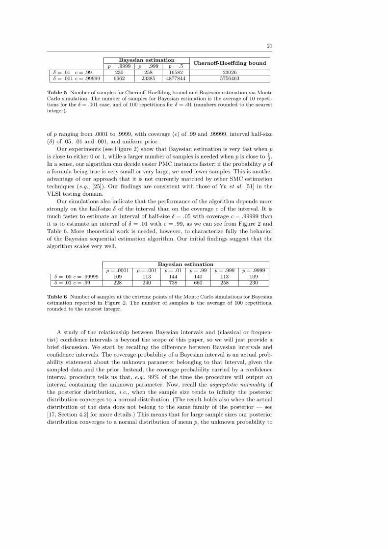
21
Bayesian estimationChernoff-Hoeffding bound
p = .9999 p = .999 p = .5δ = .01 c = .99 230 258 16582 23026δ = .001 c = .99999 6662 23385 4877844 5756463
Table 5 Number of samples for Chernoff-Hoeffding bound and Bayesian estimation via MonteCarlo simulation. The number of samples for Bayesian estimation is the average of 10 repeti-tions for the δ = .001 case, and of 100 repetitions for δ = .01 (numbers rounded to the nearestinteger).
of p ranging from .0001 to .9999, with coverage (c) of .99 and .99999, interval half-size
(δ) of .05, .01 and .001, and uniform prior.
Our experiments (see Figure 2) show that Bayesian estimation is very fast when p
is close to either 0 or 1, while a larger number of samples is needed when p is close to 12 .
In a sense, our algorithm can decide easier PMC instances faster: if the probability p of
a formula being true is very small or very large, we need fewer samples. This is another
advantage of our approach that it is not currently matched by other SMC estimation
techniques (e.g., [25]). Our findings are consistent with those of Yu et al. [51] in the
VLSI testing domain.
Our simulations also indicate that the performance of the algorithm depends more
strongly on the half-size δ of the interval than on the coverage c of the interval. It is
much faster to estimate an interval of half-size δ = .05 with coverage c = .99999 than
it is to estimate an interval of δ = .01 with c = .99, as we can see from Figure 2 and
Table 6. More theoretical work is needed, however, to characterize fully the behavior
of the Bayesian sequential estimation algorithm. Our initial findings suggest that the
algorithm scales very well.
Bayesian estimationp = .0001 p = .001 p = .01 p = .99 p = .999 p = .9999
δ = .05 c = .99999 109 113 144 140 113 109δ = .01 c = .99 228 240 738 660 258 230
Table 6 Number of samples at the extreme points of the Monte Carlo simulations for Bayesianestimation reported in Figure 2. The number of samples is the average of 100 repetitions,rounded to the nearest integer.
A study of the relationship between Bayesian intervals and (classical or frequen-
tist) confidence intervals is beyond the scope of this paper, so we will just provide a
brief discussion. We start by recalling the difference between Bayesian intervals and
confidence intervals. The coverage probability of a Bayesian interval is an actual prob-
ability statement about the unknown parameter belonging to that interval, given the
sampled data and the prior. Instead, the coverage probability carried by a confidence
interval procedure tells us that, e.g., 99% of the time the procedure will output an
interval containing the unknown parameter. Now, recall the asymptotic normality of
the posterior distribution, i.e., when the sample size tends to infinity the posterior
distribution converges to a normal distribution. (The result holds also when the actual
distribution of the data does not belong to the same family of the posterior — see
[17, Section 4.2] for more details.) This means that for large sample sizes our posterior
distribution converges to a normal distribution of mean p, the unknown probability to

22
0 0.1 0.2 0.3 0.4 0.5 0.6 0.7 0.8 0.9 10
2000
4000
6000
8000
10000
12000
14000
16000
18000
Probability p
Num
ber
of s
ampl
es
delta=.05 c=.99999delta=.01 c=.99
Fig. 2 Monte Carlo simulation for analyzing the performance of Bayesian estimation in twodifferent settings. The number of samples is the average of 100 repetitions. The probability pruns from .01 to .99 with .01 increment, plus the points .0001, .001, .999, and .9999. Uniformprior.
estimate, and variance proportional to 1n , where n is the sample size. It follows that,
asymptotically, the coverage probability of Bayesian intervals centered on the posterior
mean will be equal to that of confidence intervals computed via techniques based on
the normal distribution.
For finite (and small) sample sizes, Bayesian techniques using informative priors
can have different properties than frequentist techniques. The reason is because one
can construct arbitrarily strong priors that are quite different from the actual distribu-
tion of the data. However, it is known that by using weak (vague or non-informative)
priors, Bayesian estimates typically enjoy good frequentist properties such as coverage
probability, even for small sample sizes. In particular, this holds for the normal and
Bernoulli distributions, for which Bayesian estimation techniques can actually produce
shorter intervals than frequentist techniques [7, Section 5.6 and 5.7]. We remind that
in our experiments we have always used uniform priors, except for the experiments of
Table 2, where we have used informative priors weakly centered around the unknown
probability (estimated through our Bayesian technique).
Finally, we note that the sequential estimation technique presented in [10] is asymp-
totically “consistent” (the technique is based on an approximation of the normal dis-
tribution). That is, the coverage probability of the returned interval is guaranteed to
be the desired value only in the limit δ → 0 (interval width approaching 0). Therefore,
given a finite δ > 0 the actual coverage probability may be less than the desired value.

23
8 Related Work
Younes, Musliner and Simmons introduced the first algorithm for Statistical Model
Checking [50,49]. Their work uses the SPRT [46], which is designed for simple hy-
pothesis testing4. Specifically, the SPRT decides between the simple null hypothesis
H ′0 :M |= P=θ0(φ) against the simple alternate hypothesis H ′1 :M |= P=θ1(φ), where
θ0 < θ1. The SPRT is optimal for simple hypothesis testing, since it minimizes the
expected number of samples among all the tests satisfying the same Type I and II
errors, when either H ′0 or H ′1 is true [46]. The PMC problem is instead a choice be-
tween two composite hypotheses H0 : M |= P≥θ(φ) versus H1 : M |= P< θ(φ). The
SPRT is not defined unless θ0 6= θ1, so Younes and Simmons overcome this problem
by separating the two hypotheses by an indifference region (θ − δ, θ + δ), inside which
any answer is tolerated. Here 0 < δ < 1 is a user-specified parameter. It can be shown
that the SPRT with indifference region can be used for testing composite hypotheses,
while respecting the same Type I and II errors of a standard SPRT [46]. However, in
this case the test is no longer optimal, and the maximum expected sample size may be
much bigger than the optimal fixed-size sample test [5]. The Bayesian approach solves
instead the composite hypothesis testing problem, with no indifference region.
The method of [25] uses a fixed number of samples and estimates the probabil-
ity that the property holds as the number of satisfying traces divided by the number
of sampled traces. Their algorithm guarantees the accuracy of the results using the
Chernoff-Hoeffding bound. In particular, their algorithm can guarantee that the dif-
ference in the estimated and the true probability is less than ε, with probability ρ,
where ρ < 1 and ε > 0 are user-specified parameters. Our experimental results show a
significant advantage of our Bayesian estimation algorithm in the sample size.
Grosu and Smolka use a standard acceptance sampling technique for verifying for-
mulas in LTL [21]. Their algorithm randomly samples lassos (i.e., random walks ending
in a cycle) from a Buchi automaton in an on-the-fly fashion. The algorithm terminates
if it finds a counterexample. Otherwise, the algorithm guarantees that the probabil-
ity of finding a counterexample is less than δ, under the assumption that the true
probability that the LTL formula is true is greater than ε (δ and ε are user-specified
parameters).
Sen et al. [41] used the p-value for the null hypothesis as a statistic for hypothesis
testing. The p-value is defined as the probability of obtaining observations at least as
extreme as the one that was actually seen, given that the null hypothesis is true. It is
important to realize that a p-value is not the probability that the null hypothesis is
true. Sen et al.’s method does not have a way to control the Type I and II errors. Sen et
al. [42] have started investigating the extension of SMC to unbounded (i.e., standard)
LTL properties. Langmead [33] has applied Bayesian point estimation and SMC for
querying Dynamic Bayesian Networks.
It should be noted that with the use of abstraction, efficient tools such as Prism
[31] can verify large instances of probabilistic models using numerical (non-statistical)
techniques. Also, Prism can perform statistical model checking using the SPRT and
the Chernoff-Hoeffding bound as in [25]. Abstraction has been proposed for hybrid
4 A simple hypothesis completely specifies a distribution. For example, a Bernoulli distri-bution of parameter p is fully specified by the hypothesis p = 0.3 (or some other numericalvalue). A composite hypothesis, instead, still leaves the free parameter p in the distribution.This results, e.g., in a family of Bernoulli distributions with parameter p < 0.3.
24
systems [45], as well. However, automated abstraction is still difficult to perform in
general, and in particular for Stateflow/Simulink models.
With respect to the temporal logic used in this work, we note that our BLTL is
a sublogic of Metric Temporal Logic (MTL) [30]. In particular, MTL extends LTL
by endowing the Until operator with an interval of the positive real line with natural
endpoints (or infinite). Such intervals can also be singleton, i.e., MTL can specify that
an event happens at a particular time. For an overview of MTL, its complexity and
decidability see [36]. BLTL formulae can thus be embedded in MTL simply by assuming
that the left endpoint of any interval is 0 and the right endpoint is positive, and by
disallowing infinite endpoints.
The probabilistic logic we have defined, PBLTL, is a simple extension of BLTL
in which formulae have a single outer probabilistic quantifier. The logic PCTL [23] is
another popular probabilistic temporal formalism, which modifies (standard) CTL by
replacing in state formulae the A and E path quantifiers with probabilistic quantifiers.
In summary, PBLTL offers a more flexible logic for the temporal part (nesting of
temporal operators), while PCTL is richer on the probabilistic extension (nesting of
probabilistic operators). Also, PCTL allows unbounded Until operators.
Finally, our logics do not currently have support for rewards in the model. The
main reason is that we wanted to define a logic as general as possible, so that it could
be used on a variety of computational models. However, certain classes of models (e.g.,
Markov Decision Processes) are often associated with reward structures. Therefore, in
a statistical model checking approach to Markov Decision Processes [24], it might be
useful to extend our logic with reward operators.
9 Conclusions and Future Work
Extending our Statistical Model Checking (SMC) algorithm that uses Bayesian Se-
quential Hypothesis Testing, we have introduced the first SMC algorithm based on
Bayesian Interval Estimation. For both algorithms, we have proven analytic bounds on
the probability of returning an incorrect answer, which are crucial for understanding
the outcome of Statistical Model Checking. We have used SMC for Stateflow/Simulink
models of a fuel control system featuring fault-tolerance and hybrid behavior. Because
verification is fast in most cases, we expect SMC methods to enjoy good scalability
properties for larger Stateflow/Simulink models. Our Bayesian estimation is orders of
magnitudes faster than previous estimation-based model checking algorithms.
Acknowledgements This research was sponsored in part by the GigaScale Research Centerunder contract no. 1041377 (Princeton University), National Science Foundation under con-tracts no. CNS0926181, CNS0931985, and no. CNS1054246, Semiconductor Research Corpora-tion under contract no. 2005TJ1366, General Motors under contract no. GMCMUCRLNV301,by the US DOT award DTRT12GUTC11, and the Office of Naval Research under awardno. N000141010188. This work was carried out while P. Z. was at Carnegie Mellon University.
References
1. R. Alur, C. Courcoubetis, and D. Dill. Model-checking for probabilistic real-time systems.In ICALP, volume 510 of LNCS, pages 115–126, 1991.

25
2. C. Baier, E. M. Clarke, V. Hartonas-Garmhausen, M. Z. Kwiatkowska, and M. Ryan.Symbolic model checking for probabilistic processes. In ICALP, volume 1256 of LNCS,pages 430–440, 1997.
3. C. Baier, B. R. Haverkort, H. Hermanns, and J.-P. Katoen. Model-checking algorithmsfor continuous-time Markov chains. IEEE Trans. Software Eng., 29(6):524–541, 2003.
4. R. Beals and R. Wong. Special Functions. Cambridge University Press, 2010.5. R. Bechhofer. A note on the limiting relative efficiency of the Wald sequential probability
ratio test. J. Amer. Statist. Assoc., 55:660–663, 1960.6. M. L. Bujorianu and J. Lygeros. Towards a general theory of stochastic hybrid systems.
In H. A. P. Blom and J. Lygeros, editors, Stochastic Hybrid Systems: Theory and SafetyCritical Applications, volume 337 of Lecture Notes Contr. Inf., pages 3–30. Springer, 2006.
7. B. P. Carlin and T. A. Louis. Bayesian Methods for Data Analysis. CRC Press, Thirdedition, 2009.
8. C. G. Cassandras and J. Lygeros, editors. Stochastic Hybrid Systems. CRC, 2006.9. R. Chadha and M. Viswanathan. A counterexample-guided abstraction-refinement frame-
work for Markov decision processes. ACM Trans. Comput. Log., 12(1):1, 2010.10. Y. S. Chow and H. Robbins. On the asymptotic theory of fixed-width sequential confidence
intervals for the mean. Annals of Mathematical Statistics, 36(2):457–462, 1965.11. F. Ciesinski and M. Großer. On probabilistic computation tree logic. In Validation of
Stochastic Systems, LNCS, 2925, pages 147–188. Springer, 2004.12. D. L. Cohn. Measure Theory. Birkhauser, 1994.13. C. Courcoubetis and M. Yannakakis. The complexity of probabilistic verification. Journal
of the ACM, 42(4):857–907, 1995.14. M. H. DeGroot. Optimal Statistical Decisions. Wiley, 2004.15. P. Diaconis and D. Ylvisaker. Quantifying prior opinion. In Bayesian Statistics 2: 2nd
Valencia International Meeting, pages 133–156. Elsevier, 1985.16. B. Finkbeiner and H. Sipma. Checking finite traces using alternating automata. In Run-
time Verification (RV ’01), volume 55(2) of ENTCS, pages 44–60, 2001.17. A. Gelman, J. B. Carlin, H. S. Stern, and D. B. Rubin. Bayesian Data Analysis. Chapman
& Hall, 1997.18. M. K. Ghosh, A. Arapostathis, and S. I. Marcus. Ergodic control of switching diffusions.
SIAM J. Control Optim., 35(6):1952–1988, 1997.19. D. T. Gillespie. A general method for numerically simulating the stochastic time evolution
of coupled chemical reactions. Journal of Computational Physics, 22(4):403–434, 1976.20. H. Gong, P. Zuliani, A. Komuravelli, J. R. Faeder, and E. M. Clarke. Analysis and
verification of the HMGB1 signaling pathway. BMC Bioinformatics, 11(Suppl 7: S10),2010.
21. R. Grosu and S. Smolka. Monte Carlo Model Checking. In TACAS, volume 3440 of LNCS,pages 271–286, 2005.
22. E. M. Hahn, H. Hermanns, B. Wachter, and L. Zhang. INFAMY: An infinite-state Markovmodel checker. In CAV, pages 641–647, 2009.
23. H. Hansson and B. Jonsson. A logic for reasoning about time and reliability. Formal Asp.Comput., 6(5):512–535, 1994.
24. D. Henriques, J. Martins, P. Zuliani, A. Platzer, and E. M. Clarke. Statistical model check-ing for Markov decision processes. In QEST 2012: Proceedings of the 9th InternationalConference on Quantitative Evaluation of SysTems, pages 84–93. IEEE, 2012.
25. T. Herault, R. Lassaigne, F. Magniette, and S. Peyronnet. Approximate probabilisticmodel checking. In VMCAI, volume 2937 of LNCS, pages 73–84, 2004.
26. W. S. Hlavacek, J. R. Faeder, M. L. Blinov, R. G. Posner, M. Hucka, and W. Fontana.Rules for modeling signal-transduction system. Science STKE 2006, re6, 2006.
27. W. Hoeffding. Probability inequalities for sums of bounded random variables. J. Amer.Statist. Assoc., 58(301):13–30, 1963.
28. H. Jeffreys. Theory of Probability. Clarendon, 1961.29. S. K. Jha, E. M. Clarke, C. J. Langmead, A. Legay, A. Platzer, and P. Zuliani. A Bayesian
approach to Model Checking biological systems. In CMSB, volume 5688 of LNCS, pages218–234, 2009.
30. R. Koymans. Specifying real-time properties with metric temporal logic. Real-time Sys-tems, 2(4):255–299, 1990.
31. M. Kwiatkowska, G. Norman, and D. Parker. PRISM 4.0: Verification of probabilisticreal-time systems. In CAV, volume 6806 of LNCS, pages 585–591, 2011.
26
32. M. Z. Kwiatkowska, G. Norman, and D. Parker. Symmetry reduction for probabilisticmodel checking. In CAV, volume 4144 of LNCS, pages 234–248, 2006.
33. C. J. Langmead. Generalized queries and Bayesian statistical model checking in dynamicBayesian networks: Application to personalized medicine. In CSB, pages 201–212, 2009.
34. O. Maler and D. Nickovic. Monitoring temporal properties of continuous signals. InFORMATS, volume 3253 of LNCS, pages 152–166, 2004.
35. J. Meseguer and R. Sharykin. Specification and analysis of distributed object-basedstochastic hybrid systems. In J. P. Hespanha and A. Tiwari, editors, HSCC, volume3927, pages 460–475. Springer, 2006.
36. J. Ouaknine and J. Worrell. Some recent results in metric temporal logic. In Proc. ofFORMATS, volume 5215 of LNCS, pages 1–13, 2008.
37. A. Platzer. Stochastic differential dynamic logic for stochastic hybrid programs. InN. Bjørner and V. Sofronie-Stokkermans, editors, CADE, volume 6803 of LNCS, pages431–445. Springer, 2011.
38. A. Pnueli. The temporal logic of programs. In FOCS, pages 46–57. IEEE, 1977.39. C. P. Robert. The Bayesian Choice. Springer, 2001.40. R. Y. Rubinstein and D. P. Kroese. Simulation and the Monte Carlo Method. Wiley,
2008.41. K. Sen, M. Viswanathan, and G. Agha. Statistical model checking of black-box proba-
bilistic systems. In CAV, volume 3114 of LNCS, pages 202–215, 2004.42. K. Sen, M. Viswanathan, and G. Agha. On statistical model checking of stochastic systems.
In CAV, volume 3576 of LNCS, pages 266–280, 2005.43. A. N. Shiryaev. Probability. Springer, 1995.44. A. Tiwari. Formal semantics and analysis methods for Simulink Stateflow models. Tech-
nical report, SRI International, 2002.45. A. Tiwari. Abstractions for hybrid systems. Form. Methods Syst. Des., 32(1):57–83, 2008.46. A. Wald. Sequential tests of statistical hypotheses. Ann. Math. Statist., 16(2):117–186,
1945.47. Y.-C. Wang, A. Komuravelli, P. Zuliani, and E. M. Clarke. Analog circuit verification by
statistical model checking. In ASP-DAC 2011: Proceedings of the 16th Asia and SouthPacific Design Automation Conference, pages 1–6. IEEE, 2011.
48. H. L. S. Younes, M. Z. Kwiatkowska, G. Norman, and D. Parker. Numerical vs. statisticalprobabilistic model checking. STTT, 8(3):216–228, 2006.
49. H. L. S. Younes and D. J. Musliner. Probabilistic plan verification through acceptancesampling. In AIPS Workshop on Planning via Model Checking, pages 81–88, 2002.
50. H. L. S. Younes and R. G. Simmons. Statistical probabilistic model checking with a focuson time-bounded properties. Inf. Comput., 204(9):1368–1409, 2006.
51. P. S. Yu, C. M. Krishna, and Y.-H. Lee. Optimal design and sequential analysis of VLSItesting strategy. IEEE T. Comput., 37(3):339–347, 1988.
52. P. Zuliani, A. Platzer, and E. M. Clarke. Bayesian statistical model checking with appli-cation to Stateflow/Simulink verification. Technical Report CMU-CS-10-100, ComputerScience Department, Carnegie Mellon University, 2010.
A Appendix
A.1 Proofs
In this Section we report proofs for some of the results presented in the paper.
Lemma 1 Function K : S × B(S)→ [0, 1] is a stochastic kernel.
Proof We show that K is in fact a convex combination of two stochastic kernels. It is easy tosee that stochastic kernels are closed with respect to convex combinations.
We have already shown above that the discrete part of K, i.e., the summation term, is astochastic kernel. Because jump is a function and x is fixed, jumpe(x) is uniquely determinedfrom x and e, so the argument from above still applies. For continuous transitions, considerany (q, x) ∈ S. Then the following integralZ ∞
0Πc(q, x)(t) IB(ϕq(t, x)) dt

27
defines a probability measure over B(S). Note that Πc(q, x) is a probability density overtime, ϕq is a continuous (thus measurable) function of time, and IB is measurable since B ∈B(S) is a measurable set. Thus, the integral is well-defined and satisfies the usual probabilityrequirements for B = ∅ and B = S. Countable additivity follows easily from Lebesgue’sdominated convergence theorem. It remains to prove that, for any B ∈ B(S)
I(x) =
Z ∞0
Πc(q, x)(t) IB(ϕq(t, x)) dt
is a measurable function defined over Rn. Again, note that I(x) is finite for all x, becausethe integrand functions are all measurable and integrate up to 1. We recall that the Lebesgueintegral of a (non-negative, real) measurable function f with respect to some measure µ, isdefined as R
f dµ = supRsdµ : s simple, 0 6 s 6 f (16)
where a simple function takes only finitely many values (piecewise constant). A measurable
simple function s can be written as a finite sum s =Pli=1 ciICi
, where the ci’s are non-negative reals, and the Ci’s are disjoint measurable sets. The integral of s with respect to µ isdefined to be the finite sum Z
s dµ =
lXi=1
ciµ(Ci)
and it is easy to check that the integral does not depend on the particular representation of s.It can be shown (see for example [12, Proposition 2.3.3]) that the Lebesgue integral (16) is
equivalently defined as limi→∞Rfi dµ, where fi is any non-decreasing sequence of measur-
able simple functions that converges pointwise to f . Such a sequence can always be found [12,Proposition 2.1.7]. Finally, for any sequence gi of (non-negative, real) measurable functions,the function limi→∞ gi (with domain x | lim infi→∞ gi(x) = lim supi→∞ gi(x)), is measur-able [12, Proposition 2.1.4]. Therefore, I(·) is a measurable function. ut
Lemma 2 (Bounded sampling) The problem “σ |= φ” is well-defined and can be checkedfor BLTL formulas φ and traces σ based on only a finite prefix of σ of bounded duration.
Proof According to Lemma 3, the decision “σ |= φ” is uniquely determined (and well-defined)by considering only a prefix of σ of duration #(φ) ∈ Q≥0. By divergence of time, σ reaches orexceeds this duration #(φ) in some finite number of steps n. Let σ′ denote a finite prefix of σof length n such that
P0≤l<n tl ≥ #(φ). Again by Lemma 3, the semantics of σ′ |= φ is well-
defined because any extension σ′′ of σ′ satisfies σ′′ |= φ if and only if σ′ |= φ. Consequentlythe semantics of σ′ |= φ coincides with the semantics of σ |= φ. On the finite trace σ′, it iseasy to see that BLTL is decidable by evaluating the atomic formulas x ∼ v at each state siof the system simulation. ut
Lemma 3(BLTL on bounded simulation traces) Let φ be a BLTL formula, k ∈ N. Thenfor any two infinite traces σ = (s0, t0), (s1, t1), . . . and σ = (s0, t0), (s1, t1), . . . with
sk+I = sk+I and tk+I = tk+I ∀I ∈ N withX
0≤l<Itk+l ≤ #(φ) (17)
we have thatσk |= φ iff σk |= φ .
Proof The proof is by induction on the structure of the BLTL formula φ. IH is short forinduction hypothesis.1. If φ is of the form y ∼ v, then σk |= y ∼ v iff σk |= y ∼ v, because sk = sk by using (17)
for i = 0.2. If φ is of the form φ1 ∨ φ2, then
σk |= φ1 ∨ φ2
iff σk |= φ1 or σk |= φ2
iff σk |= φ1 or σk |= φ2 by IH as #(φ1 ∨ φ2) ≥ #(φ1) and #(φ1 ∨ φ2) ≥ #(φ2)
iff σk |= φ1 ∨ φ2
The proof is similar for ¬φ1 and φ1 ∧ φ2.

28
3. If φ is of the form φ1Utφ2, then σk |= φ1Utφ2 iff conditions (a),(b),(c) of Definition 6 hold.Those conditions are equivalent, respectively, to the following conditions (a′),(b′),(c′):
(a′)P
0≤l<i tk+l ≤ t, because #(φ1Utφ2) ≥ t such that the durations of trace σ and σ are
tk+l = tk+l for each index l with 0 ≤ l < i by assumption (17).(b′) σk+i |= φ2 by induction hypothesis as follows: We know that the traces σ and σ match at
k for duration #(φ1Utφ2) and need to show that the semantics of φ1Utφ2 matches at k.By IH we know that φ2 has the same semantics at k+i (that is σk+i |= φ2 iff σk+i |= φ2)provided that we can show that the traces σ and σ match at k + i for duration #(φ2).For this, consider any I ∈ N with
P0≤l<I tk+i+l ≤ #(φ2). Then
#(φ2) ≥X
0≤l<Itk+i+l =
X0≤l<i+I
tk+l −X
0≤l<itk+l
(a)
≥X
0≤l<i+Itk+l − t
Thus X0≤l<i+I
tk+l ≤ t+ #(φ2) ≤ t+ max(#(φ1),#(φ2)) = #(φ1Utφ2)
As I ∈ N was arbitrary, we conclude from this with assumption (17) that, indeed sI = sIand tI = tI for all I ∈ N with X
0≤l<Itk+i+l ≤ #(φ2)
Thus the IH for φ2 yields the equivalence of σk+i |= φ2 and σk+i |= φ2 when using theequivalence of (a) and (a′).
(c′) for each 0 ≤ j < i, σk+j |= φ1. The proof of equivalence to (c) is similar to that for (b′)using j < i.
The existence of an i ∈ N for which these conditions (a′), (b′), (c′) hold is equivalent toσk |= φ1Utφ2.
Theorem 1(Termination of Bayesian estimation) The Sequential Bayesian interval es-timation Algorithm 2 terminates with probability one.
Proof We follow an argument by DeGroot [14, Section 10.5]. Let p be the actual probabilitythat the BLTL formula φ holds, and let x1, . . . , xn a sample given by model checking φ over nsimulation traces (i.e., iid as the random variable X defined by (2)). Recall that the estimationalgorithm returns an interval of width 2δ which contains p with posterior probability at least c,where δ ∈ (0, 1
2) and c ∈ ( 1
2, 1) are user-specified parameters. We shall show that the posterior
probability of any open interval containing p must converge almost surely to 1, as n→∞.Let α, β > 0 be the parameters of the Beta prior. We know that the posterior Xn given
the the sample x1, . . . , xn has a Beta distribution (5) with parameters x + α and n − x + β,where x =
Pni=1 xi. Recall that the posterior mean (8) is:
E[Xn] = pn =x+ α
n+ α+ β
and the posterior variance is (see Appendix A.2):
E[(Xn − pn)2] = σ2n =
(x+ α)(n− x+ β)
(n+ α+ β)2(n+ α+ β + 1).
Because x 6 n and α, β > 0, we have that
σ2n 6
1
n+ α+ β
and thus limn→∞ σ2n = 0, i.e., the posterior variance tends to 0 as we increase the sample
size. (Intuitively, Xn will be arbitrarily close to its mean, as n → ∞.) Also, note that this iseverywhere convergence, and not just almost sure convergence.

29
Now, since α and β are fixed, from the law of large numbers it follows that
limn→∞
pn = p (almost surely) (18)
But limn→∞ σ2n = limn→∞ E[(Xn− pn)2] = 0, so Xn converges almost surely to the constant
random variable p. Therefore, the posterior probability P (Xn ∈ I) of any open interval Icontaining p must converge almost surely to 1, as n → ∞. Finally, note that the intervalreturned by the algorithm is always of fixed size 2δ > 0. ut
Theorem 2(Error bound for hypothesis testing) For any discrete random variable andprior, the probability of a Type I-II error for the Bayesian hypothesis testing algorithm 1 isbounded above by 1
T, where T is the Bayes Factor threshold given as input.
Proof We present the proof for Type I error only - for Type II it is very similar. A Type Ierror occurs when the null hypothesis H0 is true, but we reject it. We then want to boundP (reject H0 | H0). If the Bayesian algorithm 1 stops at step n, then it will accept H0 ifB(d) > T , and reject H0 if B(d) < 1
T, where d = (x1, . . . , xn) is the data sample, and the
Bayes Factor is
B(d) =P (d|H0)
P (d|H1).
The event reject H0 is formally defined as
reject H0 =[d∈ΩB(d) <
1
T∧ D = d (19)
where D is the random variable denoting a sequence of n (finite) discrete random variables,and Ω is the sample space of D - i.e., the (countable) set of all the possible realizations of D(in our case D is clearly finite). We now reason:
P (reject H0 | H0)
= (19)
P (Sd∈ΩB(d) < 1
T∧ D = d | H0)
= additivityPd∈Ω P (B(d) < 1
T∧ D = d | H0)
= independent eventsPd∈Ω P (B(d) < 1
T) · P (D = d | H0)
< B(d) < 1T
iff P (D = d | H0) < 1TP (D = d | H1)P
d∈Ω1T· P (D = d | H1)
= additivity and independence
1T· P (
Sd∈Ω D = d | H1)
= universal event
1T· P (Ω | H1) = 1
T
ut
Theorem 3(Error bound for estimation) For any discrete random variable and prior,the Type I and II errors for the output interval (t0, t1) of the Bayesian estimation Algorithm 2
are bounded above by(1−c)π0c(1−π0)
, where c is the coverage coefficient given as input and π0 is the
prior probability of the hypothesis H0 : p ∈ (t0, t1).
Proof Let (t0, t1) be the interval estimate when the estimation algorithm 2 terminates (withcoverage c). From the hypothesis
H0 : p ∈ (t0, t1) (20)
30
we compute the Bayes factor for H0 vs. the alternate hypothesis H1 : p /∈ (t0, t1). Then weuse Theorem 2 to derive the bounds on the Type I and II error. If the estimation algorithm 2terminates at step n with output t0, t1, we have that:Z
H0
f(u|x1, . . . , xn) du =
Z t1
t0
f(u|x1, . . . , xn) du > c (21)
and therefore (since the posterior is a distribution):ZH1
f(u|x1, . . . , xn) du 6 1− c. (22)
By (13) we get the Bayes factor of H0 vs H1, which can then be bounded by (21) and (22) asfollows
(1− π0)
π0·
RH0
f(u|x1, . . . , xn) duRH1
f(u|x1, . . . , xn) du>
(1− π0)
π0·
c
1− c.
Therefore, by Theorem 2 the error is bounded above by“c(1−π0)(1−c)π0
”−1=
(1−c)π0c(1−π0)
. ut
A.2 The Beta Distribution
For the reader’s convenience, we calculate the mean and variance of a random variable Y withBeta density of parameters u, v > 0. What we outline below can be found in most textbookson Bayesian statistics and special functions, e.g., [39] and [4].
Recall that the Beta density is
∀t ∈ (0, 1) g(t, u, v) b= 1
B(u, v)tu−1(1− t)v−1
where the Beta function B(u, v) is defined as:
B(u, v) b= Z 1
0tu−1(1− t)v−1dt .
It is well known that
B(u, v) =Γ (u)Γ (v)
Γ (u+ v)
where Γ (·) is Euler’s gamma function defined for z ∈ C with <(z) > 0 as:
Γ (z) b= Z ∞0
tz−1e−tdt .
Also, the gamma function satisfies the equation Γ (z + 1) = zΓ (z), for <(z) > 0. By means ofa few algebraic steps, we are now able to compute the mean of Y :
E[Y ] =1
B(u, v)
Z 1
0tu(1− t)v−1dt =
B(u+ 1, v)
B(u, v)
=Γ (u+ 1)Γ (v)
Γ (u+ 1 + v)·Γ (u+ v)
Γ (u)Γ (v)=
uΓ (u)Γ (u+ v)
(u+ v)Γ (u+ v)Γ (u)=
u
u+ v.
For the variance, we proceed analogously to show that
E[Y 2] =1
B(u, v)
Z 1
0tu+1(1− t)v−1dt =
(u+ 1)u
(u+ v + 1)(u+ v)
and thereforeV ar[Y ] = E[Y 2]− (E[Y ])2 =
uv
(u+ v)2(u+ v + 1).