Semantic Translation of Simulink/Stateflow models to Hybrid Automata

Aditya Agrawal1, Gyula Simon1 and Gabor Karsai1

1 Institute for Software Integrated Systems (ISIS), Vanderbilt University,

Nashville, TN 37203, USA {aditya.agrawal, gyula.simon, gabor.karsai }@vanderbilt.edu

Abstract. Research in the field of hybrid systems has produced a number of verification tools. Formal verification of systems is performed using such tools. In practice prototyping and simulation tools such as Matlab’s Simulink and Stateflow (MSS) are prevalent. The paper formally describes a translation process that can convert a well-defined subset of MSS into a standard form of hybrid automata. This translation process allows semantic interoperability between the industry-standard MSS tools and new verification tools developed by the research community.

1. Introduction

Model-based development of embedded systems is a process that uses explicit domain-specific constructs with well-defined semantics to represent, analyze, and synthesize a system [1]. A model should be a faithful and formal description of a system, which can be used in analysis (to determine the overall characteristics of a system), and in synthesis (to actually construct the real system).

In model-based development often a number of design tools are used that need to be integrated in a coherent framework. For example, one can consider a development process that uses Matlab Simulink/Stateflow1 (MSS) for simulation and uses a hybrid automata based tool (like, for instance, Charon [2]) for verification. MSS allows the construction of simulation models in the form of block diagrams and it has a sophisticated simulation engine. Such tools are a good choice for simulating system dynamics, but there is no support available for verifying, for instance, reachability properties (which could be highly relevant for safety-sensitive applications). System developers would like to have an automated mapping of MSS models to hybrid automata for analysis. However, the mapping between MSS and hybrid automata is not trivial.

If one wishes to use a number of design tools, semantic interoperability is of utmost importance. In order to support meaningful work, the various design tools must share semantics: the meaning of a model must be the same across multiple tools. Formally, if X and Y are design tools, and m xx M∈ and Yy Mm ∈ are models (from

1 A product of Mathworks, see www. mathworks.com .

the set of legal models Mx and My of the tools) that are used in the two tools, respectively, then the two models are semantically equivalent if and only if there exist two (semantic) mappings: SX: MX → D and SY: MY → D that map legal models into a common (semantic) domain D such that SX(mX) ≡ SY(mY). From a practical standpoint, thus the tool integration problem is reduced to (1) establishing the common semantic domain, and (2) specifying the semantic mapping.

In this paper we describe our experimental work on a semantic translator that transforms models expressed in the MSS language into Hybrid System Interchange Format (HSIF). HSIF has been developed by a community of researchers to represent dynamic networks of hybrid automata. It was designed to serve as an intermediate language for interchanging models across modeling, simulation, verification, and code generation tools. The vision is that many such tools will have an HSIF export or import capability. MSS models can be subjected to verification — provided a bridge is available between MSS and HSIF. Our goal with the work described here was to build such a bridge that preserves and carries over the semantics of models expressed in MSS into HSIF.

Both MSS and HSIF model dynamic systems. Therefore the common semantic domain D introduced above is that of dynamic network of hybrid automata (as defined by HSIF). From a practical standpoint, verification performed on HSIF models is expected to yield results that are true for the MSS models. In terms of the semantic domain this means that the models m MSSx M∈ and are semantically equivalent if given the execution semantics of MSS and HSIF they produce the same behavior. By execution semantics we mean an operational semantics defined by the time-domain behavior of the models. Verification tools must have the same execution semantics so that inferences made during the verification process can used in the context of the original system.

HSIFy Mm ∈

We posed the semantic translation problem between MSS and HSIF as follows: Given the model of a dynamic system in MSS, there exists an equivalent dynamic system model in HSIF, which produces the same execution traces. For practical reasons, we had to relax this requirement in two respects. First, while the execution semantics is mathematically precise, actual executions are never precise because of inaccuracies introduced by the finite numerical precision and finite step size in the numerical integration techniques. Therefore “same execution trace” means “the difference between execution traces is less than some ε”. Second, MSS models can have procedural (i.e. “code”) elements with side effects on global variables. Such model elements have been disallowed for the sake of simplicity. Only a restricted subset of model elements is mapped to concepts available in HSIF.

A formal specification technique (based on graph transformations) has been used to describe (and simultaneously implement) the semantic translator from MSS to HSIF. In the subsequent sections we describe the inputs and the outputs of the translator, specify the translation strategy, describe how we used it to specify the transformations, and give an illustrative example for the use of the translator.

2. The inputs and outputs of the semantic translator

2.1 The output: HSIF

HSIF is an interchange format that allows representation of the hybrid systems using dynamic networks of hybrid automata. The detailed specification is available in [3]. The individual automata in HSIF follow the definition of hybrid automata [4]. There are a finite number of locations, where each location has a number of differential and algebraic equations associated with it. The equations capture continuous time dynamics in that location, while algebraic equations describe further dependencies among variables. HSIF is capable of expressing networks of hybrid automata, where the automata can interact with each other using signals and shared variables. Signals are single writer-multiple reader variables, which are updated by one automaton and can influence multiple, other automata. Cyclic dependencies among signals are illegal, and the signal propagation among automata follows the topological order of dependencies. Interactions via shared variables are completely unrestricted: multiple writers and multiple readers are allowed on one variable.

2.2 The input: A subset of the MSS language

Simulink has a rich set of model elements (Simulink blocks) covering various areas of signal processing, while in contrast, HSIF has a strict structure with a few mathematical tools to describe hybrid systems. The translator tool cannot undertake the mission of converting every possible Simulink diagram to an equivalent hybrid automaton. Our approach is to provide a useful coverage of the element space that can be used to effectively describe hybrid systems. The MSS → HSIF translator handles a subset of Simulink blocks, which have a meaningful mapping in HSIF. The supported Simulink blocks are the following: − Continuous blocks: Integrator, State-space, Transfer Function, Zero-Pole − Mathematical operators: Product, Sum, Gain, Min/Max, and any single-

input/single-output function (Abs, Trigonometric, etc.) No logical blocks are allowed in the current implementation.

− Sources: Constant, In − Sinks: Out − Nonlinear elements: Switch − Stateflow diagrams

The supported models have certain restrictions. These restrictions are the following: (1) All Stateflow diagrams must have an initial state. (2) Side effects are only allowed in the entry action of a state. (3) Events are not supported. (4) Stateflow diagrams can receive continuous signals from the Simulink model, and provide continuous signals for the model. (5) Some of the output signals are called switching signals. A switching signal is always connected to the control input of one Switch block and only constant values may be assigned to them. (6) Switches can be controlled only by the switching signals originated from a Stateflow block, no other block can change the control input of a Switch.

The restrictions result in a clear separation of discrete and continuous behavior where all structural changes of the system are made through switches controlled by Stateflow machines. Parametrical changes can be made either by the Stateflow machine, or Simulink blocks. Logically the Simulink diagram represents the possible dynamic behaviors, while the Stateflow machines perform the reconfiguration.

The Simulink system can contain any number of Simulink sub systems or Stateflow diagrams. Stateflow diagrams can be hierarchical and can contain parallel state machines. Matlab’s implicit execution order of the parallel machines is however not taken into account during the translation process.

Since HSIF semantics enable the usage of parallel automata, the translation could produce a set of interacting automata. Unfortunately, HSIF semantics [3] require that the automata dependency graph be acyclic. In some systems it is true, in other it is not. To provide a solution for all cases, the translator creates a single automaton, where the complete system dynamics is described in each location.

3. Translation overview and Algorithms

3.1 Transformation overview

The translation from Simulink/Stateflow to HSIF requires the following logical steps: Enumeration of switching signals. The signals controlling the switches have a

special role - only these signals can change the structure of the dynamics, while other signals may affect system parameters. Hence, these switching signals need to be identified.

Transformation of states to locations. The number of locations in HSIF is determined from the Stateflow machine. Since all the switching signals originate from Stateflow, the number of locations can be determined by analyzing the (unified and flattened) state machine and switching signals.

Transformation of state transition to location transitions. The mapping of the states to locations is a one-to-many transformation. Thus, state transitions may be mapped to possibly many transitions in HSIF. Triggering condition for transitions are also mapped.

Generation of equations. Differential and algebraic equations are generated for each location based on the Simulink diagram. Since only one automaton is created, all the variables except the inputs and outputs are local variables. Stateflow variables are mapped to HSIF variables, and new variables are created to represent Simulink diagrams.

Generation of invariants. Invariants are generated from transition conditions and Stateflow variables.

Pruning unreachable locations. Unreachable locations are deleted.

3.2 The Translation Algorithm

Definition 1. The flattened and unified Stateflow state machine contains the set of states S = {s1, s2, s3, …, sN}, s1 being the initial state. The set of transitions is

where is a transition from sSST ×⊆ Tt ji ∈, i to sj. The corresponding transition condition is denoted by wi,j.

Definition 2. An output variable in the Stateflow diagram is called a switching signal if it is connected to a Control Input of a Switch block in the Simulink diagram. The set of switching signals in the state machine is Q = {q1, q2, q3, … qM}. The value of the switching signal q in state s is value(q,s). Definition 3. The switch value of a switching signal q in state s is the following:

( ) ( ) ( ) ≥

=otherwise0

, if1,

bthresholdsqvaluesqeswitchvalu , where b is the unique Switch

block connected to q. Definition 4. For a switching signal q and state si, defined(q, si) = true if either of the following conditions hold: - q is explicitly set in si, or - there exist a switch value u, such that for all j for which tj,i∈T it is true that

defined(q, sj) and switchvalue(q,sj) = u. Definition 5. The rank of state s is the number of switching signals that are defined in s. The defect of s is defined as defect(s) = N-rank(s). Definition 6. The sequence of undefined switching signals in s i is defined as

, where ( )

>=<isdefectkkkki qqqqU ,...,,,

321( ) falsesqdefined ikl

=,

)

for all l = 1, 2, …

defect(si), and . ( isdefectkkkk <<<< ...321

Translation Step 1. Each state si is split into )(2 isdefectD = locations. The set of locations generated from si is Σi={ σi,1, σi,2, … , σi,D}. Definition 7. The switch code of location σi,j is a binary sequence of length M, denoted by Ci,j = (bi,j,1, bi,j,2, …, bi,j,M). The binary values are defined as follows:

( )( )

( )

==−

∉= ,...,,, where, if,1

if,

321,,

isdefectn kkkkikk

ikikkji qqqqUqqnjbit

Uqsqeswitchvalub

The function bit(x,y) defines the yth bit of the binary representation of x, the 1st bit being the least significant bit. Definition 8. The coloring is defined on the elements of the switch code. The binary values of the code are either black or red, as follows:

∉∈

=ik

ikkji Uqblack

Uqredbcolor

if if

)( ,, .

Translation Step 2. The locations are coded and colored according to Definition 7 and Definition 8. Translation Step 3. Create a transition between σmnji ,,,τ i,n and σj,m if ti,j ∈T, and there

is no k such that bi,n,k ≠ bj,m,k and color(bj,m,k) = red. The transition guard for this transition is the predicate wi,j. Definition 9. The set of all transitions in the HSIF description is denoted by Φ. Definition 10. The Simulink diagram containing M Switch blocks describes the reconfigurable dynamic system א. The dynamic system with a particular setting of the switches with switch values x1, x2, …, xM is denoted by א(x1, x2, …, xM). Translation Step 4. For each state si copy the algebraic equations defined in the state to locations σi,j, for all j = 1, 2, 3, …, ( )isdefect2 . For each location σi,j generate the additional algebraic and differential equations of the system א(Ci,j) (see details in Section 3.3). Translation Step 5. Choose σ1,1 to be the initial location. Translation Step 6. Add the following invariants to location σi,j: - switching signal values from the entry action of si, and

- for all indices m for which there exist n such that . The

operations and ∨ are the logical not and or operations, respectively.

¬ ∨ mim

w ,

¬

Φ∈njmi ,,,τ

Definition 11. The location dependency graph is a directed graph on the set

NΣΣΣ ∪∪∪ ...21 with edges Φ. A location σ is unreachable if there is no directed path in the location dependency graph from σ1,1 to σ. Translation Step 7. Prune all unreachable locations from the HSIF description. Also delete the transitions connected to unreachable locations.

3.3 Equation generation

The differential and algebraic equations are generated for each location σi,j from the dynamic system א(Ci,j). The equation generation for location σi,j is as follows: Equation Generation Step 1. Decompose the complex linear blocks (State-space, Transfer Fn., Zero-Pole) in system א(Ci,j) to a network containing only Integrator, Sum, and Gain blocks.

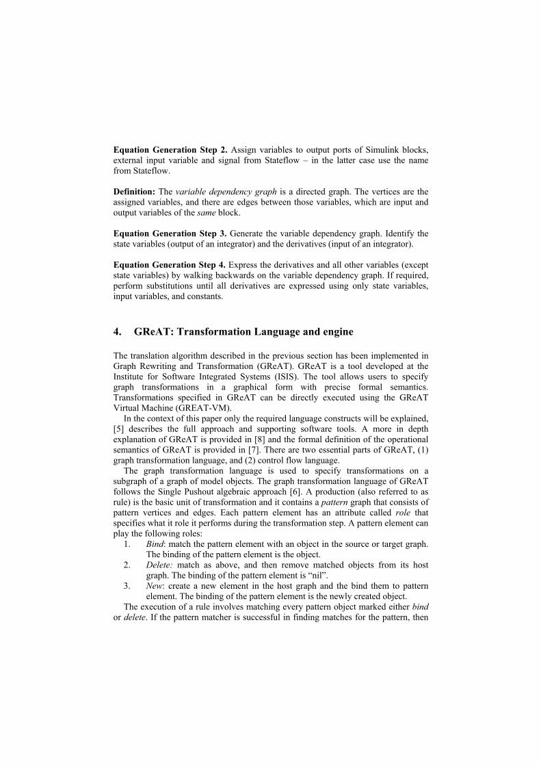
Equation Generation Step 2. Assign variables to output ports of Simulink blocks, external input variable and signal from Stateflow – in the latter case use the name from Stateflow. Definition: The variable dependency graph is a directed graph. The vertices are the assigned variables, and there are edges between those variables, which are input and output variables of the same block. Equation Generation Step 3. Generate the variable dependency graph. Identify the state variables (output of an integrator) and the derivatives (input of an integrator). Equation Generation Step 4. Express the derivatives and all other variables (except state variables) by walking backwards on the variable dependency graph. If required, perform substitutions until all derivatives are expressed using only state variables, input variables, and constants.

4. GReAT: Transformation Language and engine

The translation algorithm described in the previous section has been implemented in Graph Rewriting and Transformation (GReAT). GReAT is a tool developed at the Institute for Software Integrated Systems (ISIS). The tool allows users to specify graph transformations in a graphical form with precise formal semantics. Transformations specified in GReAT can be directly executed using the GReAT Virtual Machine (GREAT-VM).

In the context of this paper only the required language constructs will be explained, [5] describes the full approach and supporting software tools. A more in depth explanation of GReAT is provided in [8] and the formal definition of the operational semantics of GReAT is provided in [7]. There are two essential parts of GReAT, (1) graph transformation language, and (2) control flow language.

The graph transformation language is used to specify transformations on a subgraph of a graph of model objects. The graph transformation language of GReAT follows the Single Pushout algebraic approach [6]. A production (also referred to as rule) is the basic unit of transformation and it contains a pattern graph that consists of pattern vertices and edges. Each pattern element has an attribute called role that specifies what it role it performs during the transformation step. A pattern element can play the following roles:

1. Bind: match the pattern element with an object in the source or target graph. The binding of the pattern element is the object.

2. Delete: match as above, and then remove matched objects from its host graph. The binding of the pattern element is “nil”.

3. New: create a new element in the host graph and the bind them to pattern element. The binding of the pattern element is the newly created object.

The execution of a rule involves matching every pattern object marked either bind or delete. If the pattern matcher is successful in finding matches for the pattern, then

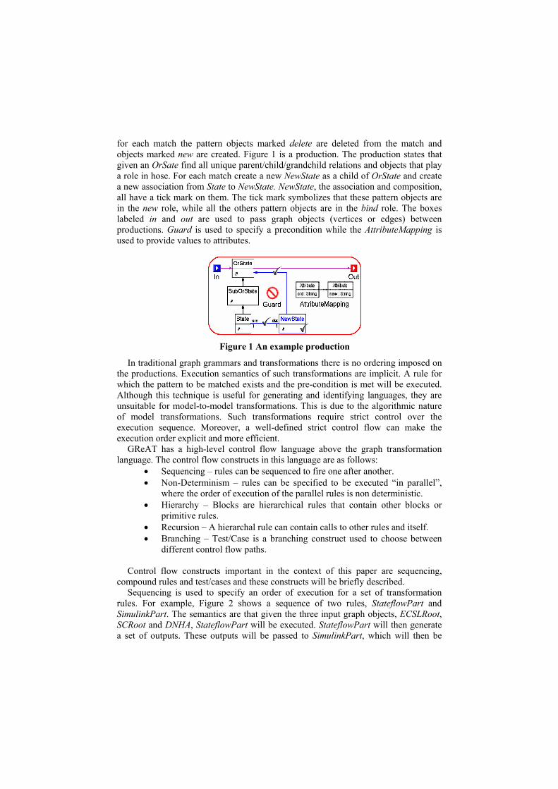
for each match the pattern objects marked delete are deleted from the match and objects marked new are created. is a production. The production states that given an OrSate find all unique parent/child/grandchild relations and objects that play a role in hose. For each match create a new NewState as a child of OrState and create a new association from State to NewState. NewState, the association and composition, all have a tick mark on them. The tick mark symbolizes that these pattern objects are in the new role, while all the others pattern objects are in the bind role. The boxes labeled in and out are used to pass graph objects (vertices or edges) between productions. Guard is used to specify a precondition while the AttributeMapping is used to provide values to attributes.

Figure 1

Figure 1 An example production

In traditional graph grammars and transformations there is no ordering imposed on the productions. Execution semantics of such transformations are implicit. A rule for which the pattern to be matched exists and the pre-condition is met will be executed. Although this technique is useful for generating and identifying languages, they are unsuitable for model-to-model transformations. This is due to the algorithmic nature of model transformations. Such transformations require strict control over the execution sequence. Moreover, a well-defined strict control flow can make the execution order explicit and more efficient.

GReAT has a high-level control flow language above the graph transformation language. The control flow constructs in this language are as follows:

• Sequencing – rules can be sequenced to fire one after another. • Non-Determinism – rules can be specified to be executed “in parallel”,

where the order of execution of the parallel rules is non deterministic. • Hierarchy – Blocks are hierarchical rules that contain other blocks or

primitive rules. • Recursion – A hierarchal rule can contain calls to other rules and itself. • Branching – Test/Case is a branching construct used to choose between

different control flow paths. Control flow constructs important in the context of this paper are sequencing,

compound rules and test/cases and these constructs will be briefly described. Sequencing is used to specify an order of execution for a set of transformation

rules. For example, shows a sequence of two rules, StateflowPart and SimulinkPart. The semantics are that given the three input graph objects, ECSLRoot, SCRoot and DNHA, StateflowPart will be executed. StateflowPart will then generate a set of outputs. These outputs will be passed to SimulinkPart, which will then be

Figure 2

executed. Hierarchy is also represented in . The sequence is contained in a compound rule called the Top-level rule. The Top-level rule contains and thus hides the behavior of the contained sequence.

Figure 2

Figure 2

Figure 2 Top-level rule of transformation

A test/case is used to choose between different transformation paths. It is similar to ‘if’ statements in traditional programming languages. In , there is a compound rule called SetImplicitValues. The rule contains a sequence with a test. TestImplicit is a test block. It contains two cases as shown in the expansion of the test. Given the three input graph objects, the test will try Case?. If Case? succeeds then the outputs will be passed to the respective output ports. If Case? Does not succeed then CaseDifferent will be tried. If CaseDifferent succeeds then the output will be passed to its respective ports. Once all inputs have been evaluated the next rules in the sequence will be executed.

Figure 5

5. Implementation of algorithms using GReAT

The algorithm is divided into two main parts. The first deals with finding all the discreet locations in the Simulink/Stateflow diagram and the second deals with inferring the continuous dynamics for each location.

5.1 Translating Stateflow

shows the top-level translation rule. The rule takes as input an MSS model graph (which is built from the MSS .MDL file), an empty State chart model and an empty hybrid automaton graph. It first deals with the Stateflow diagram and converts it to HSIF locations. Then the algorithm converts the Simulink diagram to differential equations for each location.

In the Stateflow part of the algorithm (see ), first the Stateflow models are converted into an internal representation in CreateHierarchicalStateChart. Within the internal representation the hierarchical concurrent state machine is converted to its equivalent, “flat” finite state machine in HSM2FSM. Then in CreateVarAs, associations of Simulink switches with the states are transferred to the flat machine. At this stage StateSplitting, the splitting algorithm is performed (explained in detail in next paragraph). After all the required discrete states/locations have been found, Reachibility is executed that performs reachability analysis on the models to eliminate all unreachable states. At this state we know the number of discrete states in the system and create the corresponding locations in HSIF.

Figure 3

Figure 3 The StateflowPart Rule

StateSplitting (see ) is one of the most complex parts of the mapping. It is decomposed into many stages. The first stage is Infer_Implicit_Signals and it implements Translation Step 2. This is followed by NewMachine which creates an empty state machine. The Create_State_Tribes performs state splitting based on Translation Step 1. The next step is Transfer_Transitions which implements Translation Step 3 by appropriately mapped transitions to the new machine. If the initial state was split, an initial state is selected according to Translation Step 5 in CreateInit. CarryBlockRef and In2Out perform housekeeping operations at the end.

Figure 4

Figure 4 The StateSplitting rule

Figure 4

The Infer_Implicit_Signals block in is performed repeatedly. In every iteration, for every state the SetImplicitValue rule (see ) is called. In the SetImplicitValue block all switching signals with color red are chosen. If there is an incoming transition, which alters the state of the signal, then the transition is used to infer the new state of the signal. The translator will continue the iteration until none of the signals change during a run, i.e. the iteration reaches a fixpoint. The function binds values to variables monotonically, and so it will converge to a fixed point after a finite number of iterations.

Figure 5

There are two main cases that can change the default interpretation of switching signal values. The first case is shown in . For a given State and switch variable (called Data in the diagram), if there exists another state (OtherState) with a transition to State, OtherState may influence the value of Data. Each state has a relation with Data. Relation has two attributes, color and value. Color can be either black or red, back implies that the state itself set the value while red implies that the value was inferred. Value can be {0, 1, ?, X}, where ‘?’ specifies that the state doesn’t influence data while ‘X’ specifies that the state can set the data to either ‘0’ or ‘1’.

Figure 6

Figure 5 The SetImplicitValues Rule

In Case? if State’s relation with Data is ‘red’ and value is not ‘X’ and OtherState’s relation with the Data is ‘?’ then we can infer the value of the current state’s relation with data is also ‘?’. In CaseDifferent if OtherState’s relation with Data is not ‘?’ and is not the same as State’s relation with Data. In this case the State’s relation with Data is altered according to the following rules. If State’s relation was ‘?’ then it will take OtherState’s relation. If State’s relation is not the same as OtherState’s then it will take the value of ‘X’.

Figure 6 internals of Case?

5.2 Simulink part

After all the states of the hybrid automata have been created, algebraic and differential equations need to be generated according to Translation Step 4. Various steps in this translation as described in Section 3.3 are (1) identification of state variables, (2) identification of input and output variables (3) discovery of algebraic equations for dependent variable and (4) discovery of the differential equations for the state variables.

Each integrator block in Simulink is assigned a state variable. Each input port to the entire system becomes an input variable. Each source block of Simulink also becomes an input variable. Sink blocks and output ports become output variables. Some intermediate variables are created for interfacing with Stateflow. These variables depend on other independent variables in the system.

After all the variables have been identified, the next step is to determine algebraic equations of dependent variable and differential equations for state variables. These equation differ from one location to another. Thus for each location the equations are inferred using the backward trace algorithm specified in Section 3.3.

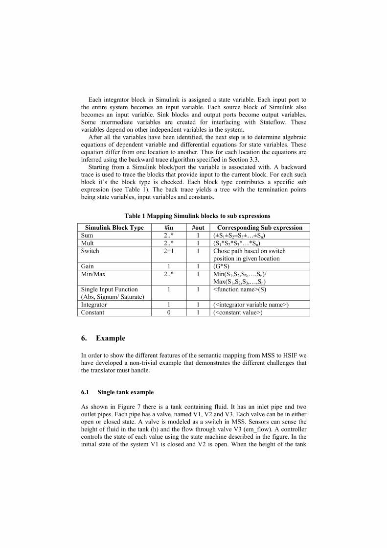
Starting from a Simulink block/port the variable is associated with. A backward trace is used to trace the blocks that provide input to the current block. For each such block it’s the block type is checked. Each block type contributes a specific sub expression (see Table 1). The back trace yields a tree with the termination points being state variables, input variables and constants.

Table 1 Mapping Simulink blocks to sub expressions

Simulink Block Type #in #out Corresponding Sub expression Sum 2..* 1 (±S1±S2±S3±…±Sn) Mult 2..* 1 (S1*S2*S3*…*Sn) Switch 2+1 1 Chose path based on switch

position in given location Gain 1 1 (G*S) Min/Max 2..* 1 Min(S1,S2,S3,…,Sn)/

Max(S1,S2,S3,…,Sn) Single Input Function (Abs, Signum/ Saturate)

1 1 <function name>(S)

Integrator 1 1 (<integrator variable name>) Constant 0 1 (<constant value>)

6. Example

In order to show the different features of the semantic mapping from MSS to HSIF we have developed a non-trivial example that demonstrates the different challenges that the translator must handle.

6.1 Single tank example

As shown in there is a tank containing fluid. It has an inlet pipe and two outlet pipes. Each pipe has a valve, named V1, V2 and V3. Each valve can be in either open or closed state. A valve is modeled as a switch in MSS. Sensors can sense the height of fluid in the tank (h) and the flow through valve V3 (em_flow). A controller controls the state of each value using the state machine described in the figure. In the initial state of the system V1 is closed and V2 is open. When the height of the tank

Figure 7

goes above 10 then outlet values V1 and V3 are opened. When the flow through V3 becomes greater that 5 the inlet value V2 is closed. The inlet V2 is opened and outlet V1 is closed when the fluid level drops below 8.

Figure 7 A single tank with three valves

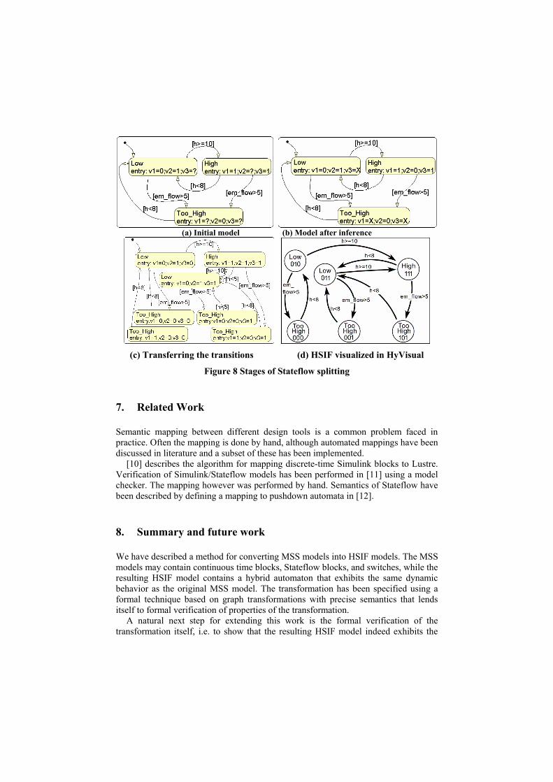
Looking at the models, the number of locations in the final hybrid automata is not apparent. Initially, in state Low, the value of V3 is undefined while the value of V2 is undefined in state High. In state Too_High the value of V1 and V3 id undefined. After running the Infer_Implicit_Signals block there are some implicit values for undefined variables. For example, in state Low, the value of V3 can be both 0 and 1, while in state High the value of V2 was fixed to 0.

After we are certain about the value of the switches in each state we can split the states that have switches with undefined values. In this example the state Low will be split into two while the state Too_High will be split into four new states (see F

(c)). igure

8

Figure 8

After the states are split, transitions from the original machine need to the transferred to the new larger machine. The algorithm takes care of mapping the transitions correctly. After the equivalent machine is created, reachability analysis is performed. Reachability analysis will reveal that state Too_High with value of V1 = 0 and V3 = 0 will never occur and it can thus be eliminated. (d) shows the locations in HSIF. The visualization is provided by HyVisual [9] a tool that can visualize and simulate HSIF models.

After all the discrete locations have been identified, the continuous time dynamics for each location need to be found. For example for location High1 the differential equation of the tank is: )15level,0max(*336level)level(dt

d −−+−=

(a) Initial model (b) Model after inference

(c) Transferring the transitions (d) HSIF visualized in HyVisual

Figure 8 Stages of Stateflow splitting

7. Related Work

Semantic mapping between different design tools is a common problem faced in practice. Often the mapping is done by hand, although automated mappings have been discussed in literature and a subset of these has been implemented.

[10] describes the algorithm for mapping discrete-time Simulink blocks to Lustre. Verification of Simulink/Stateflow models has been performed in [11] using a model checker. The mapping however was performed by hand. Semantics of Stateflow have been described by defining a mapping to pushdown automata in [12].

8. Summary and future work

We have described a method for converting MSS models into HSIF models. The MSS models may contain continuous time blocks, Stateflow blocks, and switches, while the resulting HSIF model contains a hybrid automaton that exhibits the same dynamic behavior as the original MSS model. The transformation has been specified using a formal technique based on graph transformations with precise semantics that lends itself to formal verification of properties of the transformation.

A natural next step for extending this work is the formal verification of the transformation itself, i.e. to show that the resulting HSIF model indeed exhibits the

same behavior as the original MSS model. For practical applications, more capabilities from the MSS tools could be added to the transformation, provided they are expressible in HSIF. Yet another potential work could be to extend HSIF with the capability of representing sampled-data systems, and extend the translator to map the “discrete time” blocks in MSS into the corresponding HSIF constructs. The latter one requires further research on verifying hybrid automata that also have discrete-time dynamics.

9. Acknowledgment

The DARPA/ITO MOBIES program (F30602-00-1-0580) is supporting, in part, the activities described in this paper. The authors want to thank the “HSIF semantics group”, especially R.Alur, B. Krogh, I. Lee, O. Sokolsky, and P. Varaiya for their hard work on HSIF.

10. References

[1] Janos Sztipanovits and Gabor Karsai, “Model-Integrated Computing,” IEEE Computer, pp. 110-112, April, 1997

[2] R. Alur, T. Dang, J. Esposito, R. Fierro, Y. Hur, F. Ivancic, V. Kumar, I. Lee, P. Mishra, G. Pappas, and O. Sokolsky, "Hierarchical Hybrid Modeling of Embedded Systems." Proceedings of EMSOFT'01: First Workshop on Embedded Software, October 8-10, 2001

[3] The Hybrid System Interchange Format, for details see http://www.isis.vanderbilt.edu/project/mobides/downloads.asp

[4] T. A. Henzinger. The Theory of Hybrid Automata. In Proc. of IEEE Symposium on Logic in Computer Science (LICS'96), pages 278--292. IEEE Press, 1996.

[5] Agrawal A., Karsai G., Ledeczi A., “An End-to-End Domain-Driven Software Development Framework”, Domain-Driven Development track, 18th Annual ACM SIGPLAN Conference on Object-Oriented Programming, Systems, Languages, and Applications (OOPSLA), Anaheim, California, October 26, 2003.

[6] Grzegorz Rozenberg, “Handbook of Graph Grammars and Computing by Graph Transformation”, World Scientific Publishing Co. Pte. Ltd., 1997.

[7] Karsai G., Agrawal A., Shi F., Sprinkle J., “On the Use of Graph Transformations for the Formal Specification of Model Interpreters”, Journal of Universal Computer Science, Special issue on Formal Specification of CBS, (accepted), 2003.

[8] Agrawal A., Karsai G., Shi F., “A UML-based Graph Transformation Approach for Implementing Domain-Specific Model Transformations”, International Journal on Software and Systems Modeling, (under review), 2003.

[9] Christopher Hylands, Edward A. Lee, Jiu Liu, Xiaojun Liu, Stephen Neuendorffer, Haiyang Zheng, "HyVisual: A Hybrid System Visual Modeler," Technical Memorandum UCB/ERL M03/1, University of California, Berkeley, CA 94720, January 28, 2003.

[10] P. Caspi, A. Curic, A. Maignan, C. Sofronis, S. Tripakis, "Translating Discrete-Time Simulink to Lustre", pp 84-99, Proc. of EMSOFT'03, Philadelphia, USA, 13-15 Oct., 2003.

[11] S. Sims, K. Butts, R. Cleaveland and S. Ranville, “Automated Validation Of Software Models”, 16th International Conference on Automated Software Engineering, pages 91-96, Coronado Island, California, November 2001. IEEE Computer Society Press.

[12] A. Tiwari , “Formal Semantics and Analysis methods for Simulink Stateflow Models”, Technical report, SRI International, 2002.