animals

Article

Bayesian Linear Regression Modelling for Sperm QualityParameters Using Age, Body Weight, Testicular Morphometry,and Combined Biometric Indices in Donkeys

Ana Martins-Bessa 1,2,3,* , Miguel Quaresma 1,2,3 , Belén Leiva 4, Ana Calado 1,2

and Francisco Javier Navas González 5

�����������������

Citation: Martins-Bessa, A.;

Quaresma, M.; Leiva, B.; Calado, A.;

Navas González, F.J. Bayesian Linear

Regression Modelling for Sperm

Quality Parameters Using Age, Body

Weight, Testicular Morphometry, and

Combined Biometric Indices in

Donkeys. Animals 2021, 11, 176.

https://doi.org/10.3390/

ani11010176

Received: 9 October 2020

Accepted: 14 November 2020

Published: 13 January 2021

Publisher’s Note: MDPI stays neu-

tral with regard to jurisdictional clai-

ms in published maps and institutio-

nal affiliations.

Copyright: © 2021 by the authors. Li-

censee MDPI, Basel, Switzerland.

This article is an open access article

distributed under the terms and con-

ditions of the Creative Commons At-

tribution (CC BY) license (https://

creativecommons.org/licenses/by/

4.0/).

1 Department of Veterinary Sciences, School of Agrarian and Veterinary Sciences, University of Trás-os-Montesand Alto Douro, 5000-801 Vila Real, Portugal; miguelq@utad.pt (M.Q.); anacalad@utad.pt (A.C.)

2 CECAV, Animal and Veterinary Research Center, University of Trás-os-Montes and Alto Douro,5000-801 Vila Real, Portugal

3 Veterinary Teaching Hospital, University of Trás-os-Montes and Alto Douro, Quinta de Prados,5000-801 Vila Real, Portugal

4 AEPGA-Association for the Study and Protection of Donkeys, Atenor, 5225-011 Miranda do Douro, Portugal;belenleiva.aepga@gmail.com

5 Genetics Department, Veterinary Sciences, Rabanales University Campus, University of Córdoba,Madrid-Cádiz Km. 396, 14014 Cordoba, Spain; fjng87@hotmail.com

* Correspondence: abessa@utad.pt; Tel.: +351-2593-50634

Simple Summary: The prediction of sperm output and other reproductive traits based on testicularbiometry is an important tool in the reproductive management of stallions. Nevertheless, correspond-ing research in donkeys remains scarce. Several donkey breeds in Europe face a compromising threatof extinction, which has been accelerated by the low renovation of populations and their inbreedinglevels. Although research on female reproductive physiology has made crucial advances, muchless is known about the physiology of the male. In the present work, two Bayesian models werebuilt to predict for sperm output and quality parameters in donkeys. Models included combinationsof age as a covariate and biometric and testicular measurements as independent factors. Resultsevidenced that the goodness-of-fit was similar for both models—hence, the combination of biometryand testicular factors presented improved predictive power. The application of these models mayassist in the process of making decisions in respect to the reproductive/biological, clinical, andselection handling of the animals.

Abstract: The aim of the present study is to define and compare the predictive power of two differentBayesian models for donkey sperm quality after the evaluation of linear and combined testicularbiometry indices and their relationship with age and body weight (BW). Testicular morphometrywas ultrasonographically obtained from 23 donkeys (six juveniles and 17 adults), while 40 ejaculatesfrom eight mature donkeys were analyzed for sperm output and quality assessment. Bayesianlinear regression analyses were considered to build two statistical models using gel-free volume,concentration, total sperm number, motility, total motile sperm, and morphology as dependentvariables. Predictive model 1 comprised the covariate of age and the independent factors testicularmeasurements (length, height and width), while model 2 included the covariate of age and thefactors of BW, testicular volume, and gonadosomatic ratio. Although goodness-of-fit was similar,the combination of predictors in model 1 evidenced higher likelihood to predict gel-free volume(mL), concentration (×106/mL), and motility (%). Alternatively, the combination of predictorsin model 2 evidenced higher predictive power for total sperm number (×109), morphologicallynormal spermatozoa (%), and total motile sperm count (×109). The application of the presentmodels may be useful to gather relevant information that could be used hereafter for assistedreproductive technologies.

Keywords: Bayesian models; testicular; sperm output; biometry; donkey

Animals 2021, 11, 176. https://doi.org/10.3390/ani11010176 https://www.mdpi.com/journal/animals

Animals 2021, 11, 176 2 of 23

1. Introduction

Measuring testicular size reports an approximate measurement of the amount of tes-ticular parenchyma present in a certain individual, which in turn determines the potentialfor sperm production [1,2]. Studies on equine testicular biometry are fairly common, andthe correlation between testicular dimensions and the capacity for sperm production hasfrequently been addressed in the literature, allowing the establishment of a predictiveformula for daily sperm output (DSO) [2–4]. Still, contextually, corresponding publicationson male donkey remain scarce. Besides biometric testicular data such as length, width,and volume, other factors might be investigated as independent variables (covariates) inDSO prediction, like age, body weight (BW), or the gonadosomatic ratio (GSI), which is thegonadal weight/BW ratio [5]. Previous studies evidenced that knowledge from stallionscould not be directly assumed for donkeys, as their reproductive physiology may presentsome specific particularities. For instance, donkeys present spermatogenesis cycles thatlast for 47.2 days, with each spermatogenic stage lasting for 10.5 days [6].

The numbers of the population of the Burro de Miranda’s (Equus asinus), as it occursin other donkey breeds in southern Europe countries [7], dramatically fall, with a maturemale population of around 40 jackasses and 300 breeding females. Besides, reproductionrates in such populations are low, with an excessive overuse of the same males in thepast, which derived in the occurrence of genetic bottlenecks. Although the reproductivephysiology of Miranda donkey females has already been studied [8], no research focusingon the biometry or reproductive physiology of Miranda donkey males has been reportedto date. Considering the actual population structure, the interest in applying assistedreproductive technologies (ARTs) have raised. However, the implementation of thesetechniques requires consistent knowledge of reproductive biology in order to select thebest males for ARTs programs to be successful. Testicular biometry, due to its correlationwith sperm production, is a valuable tool to estimate male fertility and is also an essentialelement of the breeding soundness evaluation (BSE). In light of the aforementioned points,the accurate prediction of sperm output and quality parameters obtained from biometricaland testicular morphometric parameters, will improve the effectiveness of reproductivemanagement in male donkeys.

In this context and bearing in mind the small but diverse mature male population,some issues in regards the statistical approach to follow may arise. For these reasons, thestatistical tools used in this study were chosen to fit the characteristics of the data to beanalyzed. According to Oravecz and Muth [9], the popularity of growth curve modelling(GCM) lies in its flexibility to simultaneously analyze within-individual changes (e.g.,changes with age, change due to intervention, due to natural changes occurring along thelife of the individuals, etc.) and between-individual effects (i.e., individual differences). Inother words, GCM may be useful to model inter-individual differences and intra-individualvariation. GCM has been successfully used to model the evolution of semen parameters inmales from other species, such as boars [10].

An individual’s specific growth trajectory, specified as a mathematical function thatdescribes how variables reciprocally relate over time, captures how an individual uniquelychanges. GCM covers situations that range from those for which the change function islinear to other occasions when curvilinear polynomial functions are fitted (for instance,quadratic, cubic, etc.), which means that modelling is not limited to consider straight-linefunctional growth. Beyond handling varying growth functions, GCM can flexibly handleunbalanced designs, meaning study individuals may be measured at different occasionsand need not be excluded from the analysis, even if some of their measurements aremissing [8].

In these regards, Bayesian inference potentiates the flexibility of GCM, given Bayesiananalyses do not assume large samples, as it would happen in maximum likelihoodestimation (either it is nonparametric or parametric inference). Besides, smaller datasets can be evaluated preventing power loss and retaining precision, as suggested byHox, et al. [11] and Lee and Song [12]. In small sample size conditions, the probability

Animals 2021, 11, 176 3 of 23

of finding significant results decreases [13]. Given power issues, this limitation oftentranslates into an increased hardness to obtain meaningful results [14].

According to Stoltzfus [15], the basic assumptions that must be met for the outputsof regression analyses to be valid include independence of errors, linearity in continuousvariables, the absence of multicollinearity, and a lack of strongly influential outliers. Addi-tionally, there should be an adequate number of events per independent variable (covariate)to avoid an overfit model. Commonly recommended minimum “rules of thumb” rangefrom 10 to 20 events per covariate. This would be supported by Chen, et al. [16], whosuggested that the usual minimum number of observations for running a linear regressionto be 30 to obtain statistically significant estimates. The same authors would even statethat sometimes this requirement cannot be met, for instance when the number of individ-uals in the sample is limited, which is common to all donkey breeds [17]. Consequently,the general rule of thumb explains that, to succeed when conducting a linear regressionanalysis, the number of observations must not be smaller than 30 or 3× (k + 1), where krepresents the number of independent variables (covariates); hence, the sample size usedin the present study fulfils all the assumptions to be used in linear regression analyses.

Contextually, Bayesian estimation methods have been reported to require a muchsmaller ratio of parameters to observations (1:3 instead of 1:5); that is, Bayesian inferencemaximizes the ability to determine significant effects for relatively limited sample sizes.These sample limitations are reflected in the broadening of confidence intervals, whichmust be accompanied by an acceptable Bayes factor value.

To the best of our knowledge, no previous study has reported an estimation of donkeysperm output and quality traits using a Bayesian approach. In this context, the aims of thepresent study are to define and compare the predictive power of two Bayesian predictivemodels for sperm quality parameters using linear testicular measurements, combinedbiometrical indices, and their relationship with age and BW as predictive factors.

2. Materials and Methods2.1. Animals

The study was carried out in the Veterinary Teaching Hospital of University of Trás-os-Montes and Alto Douro (VTH-UTAD, Vila Real, Portugal). Animals have been evaluatedwith approval and in collaboration with the Association for Study and Protection ofthe Donkey Breed Burro de Miranda (AEPGA), in the behalf of a scientific protocol ofcaooperation signed between both institutions. All animal procedures were conductedin accordance with national laws for animal welfare and experimentation as with the EUDirective 2010/63/EU for animal experiments and the approval of the Directive HospitalCommittee (Approval Ref. 408/VTH-UTAD).

Animals were clinically examined, and the genital tract was palpated previous toultrasonographic (US) evaluation. Body weight (BW) (kg) was assessed using an equinedigital floor weighting scale. For the testicular morphometric evaluation, 23 Mirandadonkeys were considered. Animals were allocated to two groups by age; juvenile toprepubertal (n = 6) (≤14 months) and mature (n = 17) (≥24 months) (Table 1). Only clinicallyhealthy animals with normal size and consistency symmetrical testis and epididymisshowing no echogenic changes in the testicular parenchyma were included. Epididymisand spermatic cords were included. Either in the juvenile or adult group, only animals withboth testicles at scrotal position were considered. For the assessment of sperm, a sub-groupof eight Miranda mature donkeys was selected from the mature group for further spermcollection and evaluation. Exams were performed during the autumn–winter season in2018–2019 (US evaluations of the juveniles); and spring–summer in 2019 (semen collectionsand US examination of adult males).

Animals 2021, 11, 176 4 of 23

Table 1. Donkeys enrolled in the study.

N Age Range Age Percentile Median Weight Evolution Per Percentile

6 7 to 14 months 14 months (P25) 200 kg11 15 to 95 months 40 months (P50/Median) 248 kg6 ≥96 months 96 months (P75) 302 kg

P25: value at 25% of observations; P50: value at 50% of observations and P75: value at 75% of observations.

2.2. Testicular Morphometry Evaluation

US testicular measurements were obtained from 23 donkeys aged from 7 to 259 monthsold and with 120 to 400 kg of weight (juvenile donkeys means: 11.17± 2.77 months old and160.33 ± 24.66 kg; mature donkeys means: 79.94 ± 50.25 months old and 279.47 ± 54.43 kg,respectively). US measurements were performed with Philips® CX30 Portable Ultrasound(Philips®, Amsterdam, Holland) with a sectorial 3.0–7.0 MHz transducer, following thepreviously described technique for stallion measurements [4]. Longitudinal and transversalplans were performed in each testicle, being the epididymis excluded from testicular USmeasurements. The electronic cursors were placed at the limit of tunica albuginea, andafter three consecutive scans, the following parameters were obtained considering thelargest measurement (cm): right and left length (L), height (H), and width (W) (cm). Rightand left testicular volume (TV) were calculated using the Lambert formula, TV = L ×W× H × 0.5233, used to measure the volume of an ellipsoid [4]. Total testicular volume(TTV), which represents the sum of the right and left TV, was obtained for each donkey. Tocompute gonadosomatic ratio (GSI) (%), i.e., testicular weight/BW, TTV (cm3) was directlyconverted into grams, based on the fact that testis volume density in mammals is very closeto one [18]. After US measurements, routine orchiectomy was performed on five juvenileand two adult donkeys. After surgery, the extirpated testis (n = 14) were measured—thesame measurements as in vivo—using precision sliding calipers.

2.3. Semen Collection and Evaluation

A sub-group of eight jackasses, ranging between 34 and 259 months of age (214–400 kg),was selected from the mature group for semen collection and further evaluation. A totalof 40 ejaculates (five ejaculates per jackass) was collected. Donkeys had been successfullyused in previous natural services. Before starting the experiment, sperm collections wereperformed for three consecutive days to minimize the number of sperm from extra-gonadalreserves, as it has been previously reported for donkeys [19]. Collections were performedat two-day intervals and using an artificial vagina (AV) (Hannover model—Minitub IbericaS.L., Tarragona, Spain) lubricated with non-spermicidal gel (ReproJelly—Minitub IbericaS.L., Tarragona, Spain), using a jenny in heat as a mount. The AV was filled with warmwater to reach and maintain an inner temperature of 50–55 ◦C. A sterile semen collectionbottle was used in each collection. The gel fraction was removed by filtering the wholeejaculate with a nylon filter (Minitub Iberica S.L., Tarragona, Spain). Gel-free ejaculatewas immediately evaluated for volume (mL), motility (%), concentration (×106/mL), andpercentage of morphologically normal (%). Volume was measured in a graduated semencollection bottle. Then, each collected ejaculate was evaluated for sperm motility and con-centration. For sperm motility evaluation, an aliquot of gel-free ejaculate was immediatelyextended 1:1 (vol/vol) with INRA 96 extender at 37 ◦C. Sperm motility was blind andsubjectively estimated by the same experienced operator after the evaluation of motilespermatozoa (%) considering five different fields under light microscopy (×200), placing asemen droplet in a prewarmed (37 ◦C) slide covered by a cover slip. Concentration wasdetermined using an improved Neubauer hemocytometer. Total sperm number (TSN,×109) was computed considering the product between the volume of gel-free ejaculatesand sperm concentration, whereas total motile sperm count (TMS, ×109) was obtained bycomputing the product between motility and TSN. Sperm morphology defects (head, inter-mediary piece, tail) were evaluated in eosin-nigrosin stained smears using light microscopyin oil immersion objective lens (×1000), counting a total of 200 sperm cells [20].

Animals 2021, 11, 176 5 of 23

2.4. Statistical Analysis2.4.1. Parametric Assumptions Testing and Approach Decision

Since sample size was a limitation in this study, parametric assumptions were testedto decide on the most appropriate statistical approach to follow to analyse the presentdata. The Shapiro–Francia W’ test (for 50 < n < 2500 samples), Shapiro–Wilk test (for n < 50samples), and Levene’s test were used to discard gross violations of parametric assumptions(normality and homoscedasticity). The Shapiro–Francia W’ test was performed using theShapiro–Francia normality routine of the test and distribution graphics package of theStata Version 15.0 software (StataCorp [21]. Supplementary Tables S1 and S2 report agross violation of normality assumption occurred in all variables of testicular biometryand sperm parameters (p < 0.01), respectively, except for gel-free volume (mL) and spermconcentration (×106/mL). Homoscedasticity was violated as well (p < 0.01); hence, anonparametric approach was suggested.

All statistical tests, including all Bayesian procedures, were performed using theexplore procedure of the descriptive statistics package in SPSS Statistics (Version 25.0, IBMCorp., Armonk, NY, USA) [22].

2.4.2. Comparative Analysis of US and Caliper Testicular Morphometry between Juvenileand Mature Jacks

Bayesian one-way ANOVA procedure was used to detect differences in the meansfor testicular measurements between juvenile and mature jackstocks using the BayesianANOVA task from the Bayesian statistics procedure of SPSS Statistics, Version 25.0, IBMCorp. [22].

2.4.3. Analysis of US Testicular Morphometry, Age and BW

Bayesian inference of Pearson’s correlation was used to characterize the posteriordistribution of the linear correlation between age and BW, US testicular measurements,and composite indices using the Pearson correlation task from the Bayesian statisticsprocedure of SPSS Statistics, Version 25.0, IBM Corp. [22]. The correlation methods usedand discussed in this paper can be validly used even if we work with repeated measures aswe tested independent data [23]. Furthermore, in case variable pairs tested held a perfectlinear correlation rxy = 1, the integral equation to perform Bayesian inference for Pearson’scorrelation would not have converged [24].

2.4.4. Analysis of US and Caliper Testicular Morphometry

Bayesian inference of Pearson’s correlation was used to characterize the posterior dis-tribution of the linear correlation between caliper testicular biometry variables(n = 14 testis) and US testicular biometry variables (n = 46 testis). The Pearson’s cor-relation coefficient measures the pairwise linear relation between the dependent variabley and the independent variable x. When rxy = |1|, the dependent variable y is perfectlylinearly correlated with the independent variable x. Then, following a decreasing or-der, a coefficient of |0.8| < rxy <|1| suggests a strong linear correlation; a coefficient of|0.3| < rxy <|0.6| suggests a moderate correlation; and a coefficient of 0 < rxy < |0.3|suggests a weak correlation, respectivelyProfillidis and Botzoris [25].

The two methods were compared to decide on whether to use US or real biometric pa-rameters or a combination of both to build Bayesian regression models. Bayesian inferencefor Pearson correlation was performed using the Pearson correlation task from the Bayesianstatistics procedure of SPSS Statistics, Version 25.0, IBM Corp. [22]. The aforementionedtest evidenced that US and caliper measuring methods were significantly correlated.

Supplementary Table S3 summarizes the estimated Pearson’s correlation pairwisecoefficients and respective Bayes factors. For all measurement pairs, the estimated Pearson’scorrelation coefficient was always higher than 0.938, with corresponding Bayes factor of<0.001. As a result, the use of US measurements was exclusively selected to integrate the

Animals 2021, 11, 176 6 of 23

models for predicting sperm output, provided measurements were taken in vivo, hencethey had a higher clinical applicability.

According to Dogan [26], although correlation analyses may erroneously detect theoccurrence of incidental relationships instead of meaningful clinical/biological association,these may be a preferable choice under certain contexts. For instance, the same authorsreported that one of the critical problems in other presumably more robust techniquessuch as the Bland–Altman analysis relies on the need for the data to meet the assumptionof a normal distribution. Contrastingly, when testing Pearson’s correlations, the pairs ofcontinuous variables need not be normally distributed, although their differences should.To determine the violation of this assumption, data may be tested against the normaldistribution using classical methods such as the Shapiro–Wilk test or the Kolmogorov–Smirnov test.

Additionally, the same authors reported the fact that the Bland–Altman analysis isnot an appropriate method to compare items for which repeated measurements wereconsidered, as in the present study. In these regards, Batterham [27] would suggest that ina spreadsheet-based simulation of calibration and validity studies, a Bland–Altman plotof difference versus mean values for the instrument and criterion may show a systematicproportional bias in the instrument’s readings, even though none is present. This artifac-tual bias arises in a Bland–Altman plot of any measures with substantial random error.In contrast, a regression analysis of the criterion versus the instrument shows no bias. Inthis context, a regression analysis also provides complete statistics for recalibrating theinstrument, if bias develops, or if random error changes since the last calibration. Conse-quently, the Bland–Altman analysis of validity should therefore be abandoned in favor ofregression, as was performed in our study.

2.4.5. Bayesian Linear Regression Modelling for Sperm Quality and Output Predictions

Gel-free volume (mL), concentration (×106/mL), TSN (×109), motility (%), morpho-logically normal (%), morphologically abnormal (%), gonadosomatic ratio (GSI) (%), andTMS (×109) were considered the dependent variables in our study. Two separate statisticalmodels were built, in which the predictive power of combinations of certain independentfactors was evaluated.

Each of the regression models used in this study followed the general equationyi = X1β1 + . . . Xiβi + εi, where i = 1,2, . . . i is the ith number of factors; yi is the vectorof records for the aforementioned dependent variables with dimension n (217 recordsbelonging to 31 jacks); Xi is the appropriate incidence matrix for factors; and βi are thestandardized regression coefficients for the ith number of factors and covariates con-sidered, respectively. The general regression equation for model 1 was Y = Intercept +βage (months)·age (months) + βLength LT (cm)·length LT (cm) + βLength RT (cm) ·length RT (cm)+ βHeight LT (cm)· height LT (cm) + βHeight RT (cm)· height RT (cm) + βWidth LT (cm)· width LT(cm) + βWidth RT (cm)·width RT (cm). Oppositely, the general regression equation for model2 was Y = Intercept + βAge (months)·Age (months) + βBW (kg)· BW (kg) + βTTV (cm3)·TTV(cm3) + βGSI·GSI, except for gonadosomatic ratio (GSI) (%), for which the last term in theequation was not included, provided this term refers to gonadosomatic ratio (GSI) (%)itself (βGSI·GSI).

According to Carlin [28], Bayesian inferences are sensitive to the dependence ofvariables on time (conditional on θ and x). If such dependence is large, it needs to bemodeled, or the inferences will not be appropriate. For this reason, age was consideredin the models. Under this design, time (age) plays a similar role to a blocking variable orcovariable. For example, suppose that E(y|x, θ) has a linear trend in time (age) but thatthis dependence is not modeled (that is, suppose that a model is fit ignoring time (age)).Then, posterior means of factors or covariables in the model will tend to be reasonable,but posterior standard deviations will be too large, because this design yields treatmentassignments that, compared to complete randomization, tend to be more balanced fortime (age).

Animals 2021, 11, 176 7 of 23

As Brewer [29] suggested, in our case, the use of an intercept was necessary as anempirical need for it was detected (for instance when unstandardized coefficients are usedas in the present study). In these regards, confidence intervals for the estimated interceptwere used as empirical indicators for the need of the intercept. Residual effects (εi) wereassumed to follow a normal distribution as εi|XiN

(0, σ2

εi), where Xεi is an identity matrix

and σ2εi is residual variance, respectively. For a continuous predictor variable, such as those

in the present study, unstandardized coefficients are produced by the linear regressionmodel using the independent variables measured in their original scales.

Unstandardized coefficients βi can be interpreted considering what was stated byHayes, et al. [30]—that all other variables being held constant, an increase of one unit inXi is associated with an average increase of βi units in Y. In the sections below, a detailedsummary of the priors and posterior distributions used in this study is reported. A fulldescription of the algorithms used by SPSS to perform Bayesian Inference on MultipleLinear Regression Models in this study can be found in the public document IBM SPSSStatistics Algorithms v. 25.0. by IBM Corp. [24].

When large number of parameters are being considered in a model, quadratic ap-proximation has been reported to be computationally faster in terms of discretization andcomputing the likelihood over all possible parameter combinations compared to otherapproximations such as the Markov Chain Monte Carlo (MCMC) methods used in thisstudy. However, the use of this quadratic approach was not feasible given it assumesthe posterior distribution follows a normal distribution. In the context of our data, thisassumption cannot be presumed provided the gross violation reported for the distributionproperties reported at previous assumption testing stage.

After Bayesian Pearson’s correlation coefficients across variables had been performed,two distinct combinations of factors were evaluated. First, model 1 comprised the covariateof age (months) and the independent factors of LLT (length of left testicle) (cm), LRT (lengthof right testicle) (cm), HLT (length of left testicle) (cm), HRT (height of right testicle) (cm),WLT (cm) (width of left testicle), and WRT (width of right testicle) (cm). Second, model2 comprised the covariate of age (months) and the factors BW (kg), TTV (total testicularvolume) (cm3) and GSI (%). Lowest correlations were found for age and any of the restof variables, hence, the covariate was retained in both models. The value of almost 1 forthe correlation found between VLT (cm3) (volume of left testicle) and VRT (volume ofright testicle) (cm3) and TTV (cm3) was the basis to decide on using composite TTV (cm3),given the reduced number of variables in model 2. BW was only considered in model 2,given the high generalized close to or above 0.9 correlations that it held with biometriccaliper measurements. Bayesian linear regression analyses were performed using thelinear regression package from the Bayesian statistics task of SPSS Statistics, Version 25.0,IBM Corp. [22]. The Bayesian Linear Regression test routine of the linear regression andrelated package of the Stata Version 16.0 software process was used to compute posteriordistribution statistics for each factor included in each model to predict for each dependentvariable. Once the analysis had been performed, we interpreted the estimated effect of thefactors considered in the resulting predictive models, their confidence intervals, and theposterior distribution statistics.

2.4.6. Jeffrey–Zellner–Siow (JZS) Mixture of g-Priors

For the present analyses, the Jeffrey–Zellner–Siow mixture of g-priors [31] was used.Jeffrey–Zellner–Siow’s prior somehow appears as a data-dependent prior through itsdependence on Xi, but this has been reported not to be a drawback since regression modelsare conditional on Xi. As suggested by Heck [32], JZS prior could be an alternative thatmay satisfy several theoretical requirements such as the equality constraint on the test-relevant parameters, for instance of β, which leads to the null hypothesis H0 = β = β0 [33].The benefits of JSZ prior distribution had also been reported by Rouder, et al. [34] andLiang, et al. [31]. Contextually, conditional on the residual variance (σ2

εi), the JZS prior

Animals 2021, 11, 176 8 of 23

defines a multivariate Cauchy distribution for the slope parameters of the full model,as follows

(βi|σ2εi) ∼ MVC

(0P,γi

2σ2εiCi

−1), which is defined by a P-dimensional zero vector(location vector) and a scale matrix. The constant γi determines the amount of scaling,which is chosen by the user a priori, the residual variance σ2

εi, and the matrix Ci = X′iXi/Ni,which is the covariance matrix of the centred design matrix Xi.

There are qualities of the JZS prior [34] that make it especially appropriate whenperforming linear regression analyses. Among these, the prior is symmetric and centeredat zero in line with the predictive matching criterion as reported by Bayarri, et al. [35].As a result, positive and negative values of the slope parameters have a priori the sameprobability to occur. Furthermore, JZS prior is scale invariant, thus the resulting Bayesfactor does not depend on the scale of both the dependent variable and factors or covariates,hence results do not change when different unit variables are evaluated together, which iscommon in field conditions studies.

This independence from the measurements of model elements is achieved by scalingthe multivariate Cauchy distribution by the residual variance σ2

εi (a priori, a larger residualvariance implies larger slopes) and by the inverse of the covariance matrix Ci (a priori,a covariate with a larger variance implies smaller slopes). It may be worth consideringthat the procedure of defining a scaled prior for unstandardized coefficients (βi) equals theprocess of defining a prior for standardized coefficients (β∗i ) [34].

Third, the scale parameter γ is fixed to a constant by the user, which allows priorbeliefs to be specified about the expected effect size. IBM Corp. [24] algorithm guide reportsthat the algorithm of JZS prior for linear regression analyses, to compute the Bayes Factoruses the default value of γ = 2

√π = 3.5, which reflects a prior belief of a medium effect

size. For a single covariate x, this choice implies that the standardized regression slopeβ∗i = βi· SD(xi)/σi has an a priori probability of 53.2% of being in the range [−0.50, +0.50].

Authors such as Rouder and Morey [36] also reported additional theoretical advan-tages of the JZS prior, such as its consistency in model selection (the fact that the Bayesfactor, goes to infinity as the number of observations N increases without bound-favoringthe data-generating model) or consistency in information (the Bayes factor for a certaineffect goes to infinity as the proportion of explained variance or R Squared (R2) increasesto 1). Additionally, Bayes factors for JZS prior can be relatively easily and highly preciselycomputed [37] and has been adapted for the default t-test [38], ANOVA [34], and linearregression [32].

2.4.7. Factor and Covariate Effects Bayesian Modelling (FCEBM)

Being yi, any of the effects of any of the independent variables (covariates) consideredin this study, the posterior distribution of yi in the context of the data D is

p(yi/D) =i

∑i = 20

p(yi|Mi, D) p(Mi|D)

This is an average of the posterior distributions of each model, weighted by thecorresponding posterior model probabilities. In the previous equation, the posteriorpredictive distribution of yi given a particular model Mi is

p(yi|MiD) =∫

p(yi|βi, Mi, D)p(βi|MiD)dβi

and the posterior probability of model Mi is given by

p(Mi|D) =p(D|Mi)p(Mi)

∑ii = 20 p(D|Mi)p(Mi)

Animals 2021, 11, 176 9 of 23

wherep(Mi|D) =

∫p(D|βi, Mi)p(βi|Mi)dβi

is the integrated likelihood of model Mi, βi is the vector of parameters of model Mi, p(βi|Mi)is prior density of βi under model Mi, p(D|βi|Mi) is the likelihood, and p(Mi) is the priorprobability that Mi is the true model.

For a problem with P potential covariates, the number of models, K, can be enormous(K = 2P in the absence of other constraints). Only a small number of these models will havemuch support from the data, thus be selected by SPSS for each covariate. Marginal posteriordistributions of all unknowns were estimated using the Gibbs sampling algorithm.

2.4.8. Factors and Covariate Effect Bayesian Interpretation (CEBI)

The checklist proposed by Depaoli and Van de Schoot [39] was used to detect issuesto check before estimating the model, (b) issues to check after estimating the model butbefore interpreting results, (c) understanding the influence of priors, and (d) actions to takeafter interpreting results.

Interpreting the effect of each particular covariate (independent variables used in thisstudy) can be made as follows.

First, the posterior probability p[β∗i 6= 0/D] expresses the likelihood that the factoror covariate has an effect on each particular variable. Standard rules of thumb [40] forinterpreting this posterior probability are as follows: <50% evidence against the effect;50–75% weak evidence for the effect; 75–95% positive evidence; 95–99% strong evidence;>99% very strong evidence, whose results are comparable to commonly used thresholds todefine significance of evidence through Bayes factor (BF) as reported in SupplementaryTable S4.

Second, posterior distribution estimates (means) are used to measure the magnitudeof the effect of a particular factor and covariate. For continuous predictor variables (metriccovariates), such as the numeric variables used in this study, the regression coefficientrepresents the difference in the predicted value of the response variable for each one-unitchange in the predictor variable, assuming all other predictor variables are held constant.When response variables are metric and can readily be interpreted in terms of impact, suchas the ones in our study, β regression coefficients effect sizes by themselves.

Third, the 95% credibility interval shows that there is a 95% probability that theseregression coefficients (posterior distribution mean value for each covariate and factor) inthe population lie within the corresponding credibility intervals. When 0 is not containedin the credibility interval, a significant effect for such factor is detected.

Supplementary Table S5 report a summary of posterior distribution statistics fromBayesian unstandardized linear (β) regression coefficients for each of the aforementionedvariables considered in the analyses and a summary of Bayesian ANOVA outputs to testfor differences in the means for US and caliper testicular measurements between juvenile(n = 6) and mature donkeys (n = 17).

2.4.9. Convergence Criterion

The rounds of iteration continued until a tolerance convergence criterion of 10−8

was reached as suggested in literature [41]. Once the convergence criterion was reached,initial parameters were set, and model fitting properties were evaluated. The maximumnumber of iteration rounds used for each analysis was 2000 as suggested in IBM SPSSStatistics Algorithms version 25.0 by IBM Corp. [24]. This convergence criterion was chosenprovided it has been used in Bayesian ANOVA and linear regression analyses in researchcontexts of limited sample sizes [42].

Animals 2021, 11, 176 10 of 23

2.4.10. Model Validity, Explanatory Power of Present Data, and Predictive Power ofFuture Data

The process of validation and comparison of Bayesian model is fully mathematicallydescribed in Geweke [43]. In this context, some authors [44] have suggested a correct prooffor model validation should be based on the mean square error (MSE) of the models beingevaluated. Additionally, although mean square residual or error (MSE) and minimummean-square residual or error (MMSE) have been used and widely reported to measurehow close a regression line is to a set of points (how good a certain model fits the databeing observed), mean square prediction error or MSPE (= RSS/no. of observations) waschosen to measure error variation given MSE has been reported to be influenced by thenumber of predictors [26] in cases of reduced sample sizes [45,46].

Residual sum of squares (RSS) measures the amount of variance in a data set that isnot explained by a regression model. That is, if we consider a regression to be a measure ofthe strength of the relationship between a dependent variable and an independent variablefrom a set of independent variables, then the RSS measures the amount of error remainingbetween the regression function and the data set—hence, it essentially determines howwell a regression model explains or represents the data in the model. A smaller RSS figurerepresents a better suitability of the regression function to model for the data that it isintended to model.

In Bayesian inference, Monte Carlo Standard Error (MCSE) is another measure ofaccuracy of the chains. It is defined as the standard deviation of the chains divided bytheir effective sample size. MCSE has been reported to be the nonparametric or Bayesiancounterpart of MSPE, and has been suggested to be used as the validation criteria inBayesian Linear Regression model comparison studies [47].

Bayes factor (BF) provides an indirect measure of the explanatory power of the modelto describe presently observed data (in our study). Larger BFs imply higher likelihoods forthe combination of factors considered to explain the response variables being modelled.Commonly used thresholds to define significance of evidence following the premises byJeffreys [48] and Lee and Wagenmakers [49] are reported in Table S4. Intrinsically relatedto BF, Bayesian R2 can be considered as a data-based estimate of the proportion of varianceexplained for data. Additionally, acceptance rate, efficiency, and Monte Carlo standarderror (MCSE) were used to determine the validity of the Bayesian methods implemented.Supplementary Table S4 reports a summary of the description and interpretation of eachmodel validity parameter used. Bayesian statistics predictive accuracy of the model [50]can be estimated through posterior predictive checking [51] (Supplementary Table S6).

BIC was then calculated, as it explains how well the model will predict on new data.Bayesian information criterion (BIC) or Schwarz information criterion (also SIC, SBC, SBIC)was computed as follows:

BIC = N ∗N ln(MSPE) + K ∗ ln(N) (1)

where MSPE is the mean squared prediction error, N is the number of observations orrecords, and K is the number of independent parameters of the model.

BIC was evaluated to compare predictive power across models. To summarize, BICconsiders both the statistical goodness of fit and the number of parameters that have tobe estimated to achieve this particular degree of fit, by imposing a penalty the numberof parameters is increased [52,53]. BIC measures the trade-off between model fit andcomplexity of the model to determine [54]. Lower BIC values suggest that a particularmodel should have improved prediction properties in comparison to models for whichhigher values have been reported. In these regards, Bayesian R2 answers a differentquestion as Bayesian R2 estimates the explanatory power of observed data, when the modelis regression and non-adjusted R2 is used.

Animals 2021, 11, 176 11 of 23

Frequently, when more variables are added, model predictive accuracy decreases.Consequently, a model with higher R2 will have higher-hence, worse-BIC values. Theaddition of “noise” variables to the fit (for which a relationship has not been suggested)will increase R2 values, but it will also decrease predictive power of the model. Hence, themodel with more “noise” variables will have higher R2 and higher BIC.

3. Results3.1. Descriptive Analysis for US Testicular Morphometry, Combined Biometric Indices andSperm Output

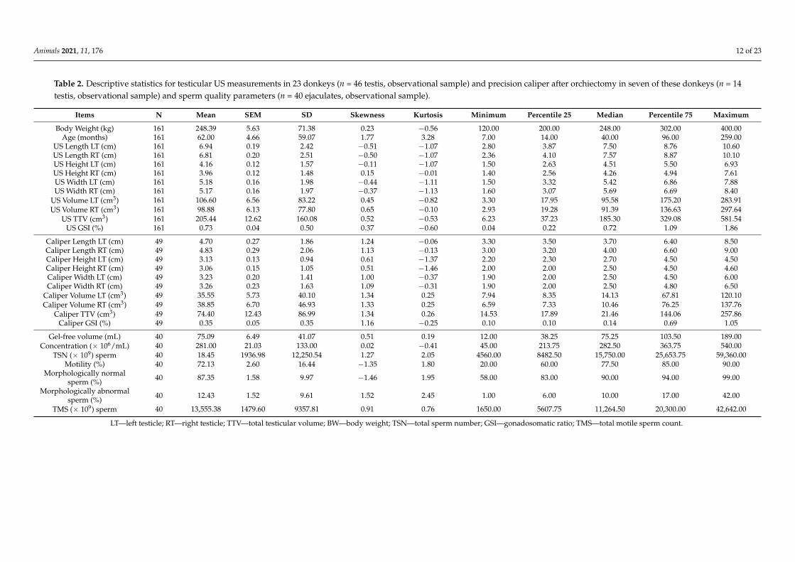
Table 2 reports a summary of the descriptive statistics for age, BW, ultrasonographic(US) and caliper testicular morphometry (cm); L, H, W, TTV, GSI for juvenile and maturedonkeys (n = 46 testis). Descriptive statistics of US and caliper measurements were com-puted for each group to perform a comparative analysis (Supplementary Table S7a,b). Inthe juvenile group, mean TTV (cm3) was 17.74 ± 9.89 (n = 12 testis), while in mature group,TTV (cm3) was 271.69 ± 133.21 (n = 34 testis).

In the juvenile group, there was a progressive increase in all US testicular measure-ments, namely in TTV, from seven to 24 months, which was especially noticeable after11 months of age. At 12–14 months, mean TTV was 21.05 ± 9.30 cm3 (n = 10 testis), and at24–26 months, TTV was 85.27 ± 18.66 cm3 (n = 4 testis) (P < 0.01). Additionally, an increasein TTV was described after 150 kg of BW had been attained, which was verified in alldonkeys after 12 months. On the other hand, after 168 months of age, a gradual decrease inTTV was noted. No difference between left and right testicle was found. Gonadosomaticratio (GSI) (%) means in juveniles was 0.11 ± 0.06 and in matures 0.95 ± 0.39. Significantdifferences (p < 0.001) were found between juvenile and mature groups for all testicularbiometrical parameters (Table S5).

Results of sperm output and quality parameters (n = 40 ejaculates, observational unit);gel-free volume (mL), motility (%), concentration (×106/mL), TSN (×109), TMS (×109),normal and abnormal sperm morphology (%) are presented in Table 1. TSN and TMSmeans was 18.453± 1.936× 109 sperm and 13.555± 1.479× 109 motile sperm, respectively.Sperm morphological abnormalities description can be consulted in Table S8.

3.2. Statistical Analyses3.2.1. Bayesian Pearson’s Correlation Coefficients Preliminary Testing

Following a probabilistic view of regression, it can be assumed that any dependentvariable (Y) has a certain associated variance σ2. Linear regression bases on identifying theweight vector from observed data of a dependent variable to then use it to make predictions.For the model to be stable enough, the variance of the weight vector (Wls) should be low.If weight vectors variance is high, it means that the model is very sensitive to data. Theweights differ largely with observed data if the variance is high. This means that the modelmight not perform well with observed data. When highly correlated covariables are usedin regression models, the variance of the weight vector will be large. This occurs becausewhen highly correlated features (covariates or factors) are considered, the values in theSingular Value Decomposition “S” matrix will be small. Hence inverse square of “S” matrix(S−2) will be large which makes the variance of Wls large. For these reasons, Pearson’scorrelation coefficients must be tested prior to performing regression analyses.

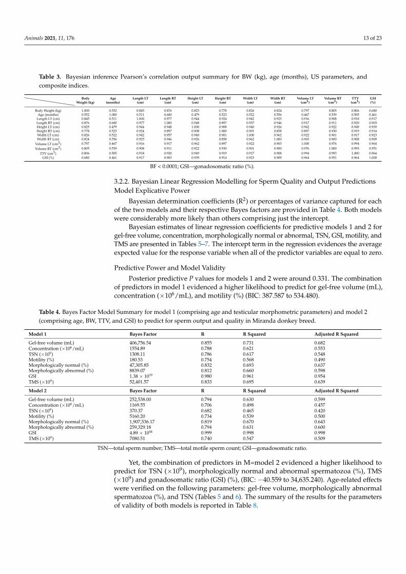
Table 3 summarizes the estimated sample Pearson’s correlation coefficient and theBayes factors for BW (kg), age (months), US testicular biometric parameters and compositeindices. For all variable pairs, the estimated Pearson’s correlation coefficient was alwayshigher than 0.461, with a corresponding Bayes factor of <0.001, in all cases. Besides,moderate to high Bayesian inference Pearson’s correlation coefficients were found betweenage, BW, and testicular biometric variables. Pearson’s correlation coefficients betweentesticular biometry and BW were always >0.778, whereas Pearson’s correlation coefficientsbetween testicular biometry and age were >0.467.

Animals 2021, 11, 176 12 of 23

Table 2. Descriptive statistics for testicular US measurements in 23 donkeys (n = 46 testis, observational sample) and precision caliper after orchiectomy in seven of these donkeys (n = 14testis, observational sample) and sperm quality parameters (n = 40 ejaculates, observational sample).

Items N Mean SEM SD Skewness Kurtosis Minimum Percentile 25 Median Percentile 75 Maximum

Body Weight (kg) 161 248.39 5.63 71.38 0.23 −0.56 120.00 200.00 248.00 302.00 400.00Age (months) 161 62.00 4.66 59.07 1.77 3.28 7.00 14.00 40.00 96.00 259.00

US Length LT (cm) 161 6.94 0.19 2.42 −0.51 −1.07 2.80 3.87 7.50 8.76 10.60US Length RT (cm) 161 6.81 0.20 2.51 −0.50 −1.07 2.36 4.10 7.57 8.87 10.10US Height LT (cm) 161 4.16 0.12 1.57 −0.11 −1.07 1.50 2.63 4.51 5.50 6.93US Height RT (cm) 161 3.96 0.12 1.48 0.15 −0.01 1.40 2.56 4.26 4.94 7.61US Width LT (cm) 161 5.18 0.16 1.98 −0.44 −1.11 1.50 3.32 5.42 6.86 7.88US Width RT (cm) 161 5.17 0.16 1.97 −0.37 −1.13 1.60 3.07 5.69 6.69 8.40

US Volume LT (cm3) 161 106.60 6.56 83.22 0.45 −0.82 3.30 17.95 95.58 175.20 283.91US Volume RT (cm3) 161 98.88 6.13 77.80 0.65 −0.10 2.93 19.28 91.39 136.63 297.64

US TTV (cm3) 161 205.44 12.62 160.08 0.52 −0.53 6.23 37.23 185.30 329.08 581.54US GSI (%) 161 0.73 0.04 0.50 0.37 −0.60 0.04 0.22 0.72 1.09 1.86

Caliper Length LT (cm) 49 4.70 0.27 1.86 1.24 −0.06 3.30 3.50 3.70 6.40 8.50Caliper Length RT (cm) 49 4.83 0.29 2.06 1.13 −0.13 3.00 3.20 4.00 6.60 9.00Caliper Height LT (cm) 49 3.13 0.13 0.94 0.61 −1.37 2.20 2.30 2.70 4.50 4.50Caliper Height RT (cm) 49 3.06 0.15 1.05 0.51 −1.46 2.00 2.00 2.50 4.50 4.60Caliper Width LT (cm) 49 3.23 0.20 1.41 1.00 −0.37 1.90 2.00 2.50 4.50 6.00Caliper Width RT (cm) 49 3.26 0.23 1.63 1.09 −0.31 1.90 2.00 2.50 4.80 6.50

Caliper Volume LT (cm3) 49 35.55 5.73 40.10 1.34 0.25 7.94 8.35 14.13 67.81 120.10Caliper Volume RT (cm3) 49 38.85 6.70 46.93 1.33 0.25 6.59 7.33 10.46 76.25 137.76

Caliper TTV (cm3) 49 74.40 12.43 86.99 1.34 0.26 14.53 17.89 21.46 144.06 257.86Caliper GSI (%) 49 0.35 0.05 0.35 1.16 −0.25 0.10 0.10 0.14 0.69 1.05

Gel-free volume (mL) 40 75.09 6.49 41.07 0.51 0.19 12.00 38.25 75.25 103.50 189.00Concentration (× 106/mL) 40 281.00 21.03 133.00 0.02 −0.41 45.00 213.75 282.50 363.75 540.00

TSN (× 109) sperm 40 18.45 1936.98 12,250.54 1.27 2.05 4560.00 8482.50 15,750.00 25,653.75 59,360.00Motility (%) 40 72.13 2.60 16.44 −1.35 1.80 20.00 60.00 77.50 85.00 90.00

Morphologically normalsperm (%) 40 87.35 1.58 9.97 −1.46 1.95 58.00 83.00 90.00 94.00 99.00

Morphologically abnormalsperm (%) 40 12.43 1.52 9.61 1.52 2.45 1.00 6.00 10.00 17.00 42.00

TMS (× 109) sperm 40 13,555.38 1479.60 9357.81 0.91 0.76 1650.00 5607.75 11,264.50 20,300.00 42,642.00

LT—left testicle; RT—right testicle; TTV—total testicular volume; BW—body weight; TSN—total sperm number; GSI—gonadosomatic ratio; TMS—total motile sperm count.

Animals 2021, 11, 176 13 of 23

Table 3. Bayesian inference Pearson’s correlation output summary for BW (kg), age (months), US parameters, andcomposite indices.

BodyWeight (kg)

Age(months)

Length LT(cm)

Length RT(cm)

Height LT(cm)

Height RT(cm)

Width LT(cm)

Width RT(cm)

Volume LT(cm3)

Volume RT(cm3)

TTV(cm3)

GSI(%)

Body Weight (kg) 1.000 0.552 0.845 0.876 0.825 0.778 0.826 0.824 0.797 0.805 0.806 0.680Age (months) 0.552 1.000 0.511 0.600 0.479 0.523 0.522 0.556 0.467 0.539 0.505 0.461

Length LT (cm) 0.845 0.511 1.000 0.977 0.944 0.924 0.942 0.925 0.916 0.908 0.918 0.917Length RT (cm) 0.876 0.600 0.977 1.000 0.948 0.897 0.957 0.946 0.917 0.911 0.920 0.903Height LT (cm) 0.825 0.479 0.944 0.948 1.000 0.908 0.940 0.926 0.962 0.922 0.949 0.939Height RT (cm) 0.778 0.523 0.924 0.897 0.908 1.000 0.901 0.858 0.897 0.930 0.919 0.914Width LT (cm) 0.826 0.522 0.942 0.957 0.940 0.901 1.000 0.962 0.922 0.901 0.917 0.923Width RT (cm) 0.824 0.556 0.925 0.946 0.926 0.858 0.962 1.000 0.903 0.900 0.908 0.909

Volume LT (cm3) 0.797 0.467 0.916 0.917 0.962 0.897 0.922 0.903 1.000 0.976 0.994 0.964Volume RT (cm3) 0.805 0.539 0.908 0.911 0.922 0.930 0.901 0.900 0.976 1.000 0.993 0.951

TTV (cm3) 0.806 0.505 0.918 0.920 0.949 0.919 0.917 0.908 0.994 0.993 1.000 0.964GSI (%) 0.680 0.461 0.917 0.903 0.939 0.914 0.923 0.909 0.964 0.951 0.964 1.000

BF < 0.0001; GSI—gonadosomatic ratio (%).

3.2.2. Bayesian Linear Regression Modelling for Sperm Quality and Output PredictionsModel Explicative Power

Bayesian determination coefficients (R2) or percentages of variance captured for eachof the two models and their respective Bayes factors are provided in Table 4. Both modelswere considerably more likely than others comprising just the intercept.

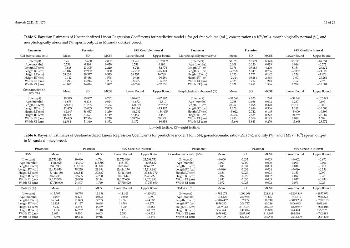
Bayesian estimates of linear regression coefficients for predictive models 1 and 2 forgel-free volume, concentration, morphologically normal or abnormal, TSN, GSI, motility, andTMS are presented in Tables 5–7. The intercept term in the regression evidences the averageexpected value for the response variable when all of the predictor variables are equal to zero.

Predictive Power and Model Validity

Posterior predictive P values for models 1 and 2 were around 0.331. The combinationof predictors in model 1 evidenced a higher likelihood to predict for gel-free volume (mL),concentration (×106/mL), and motility (%) (BIC: 387.587 to 534.480).

Table 4. Bayes Factor Model Summary for model 1 (comprising age and testicular morphometric parameters) and model 2(comprising age, BW, TTV, and GSI) to predict for sperm output and quality in Miranda donkey breed.

Model 1 Bayes Factor R R Squared Adjusted R Squared

Gel-free volume (mL) 406,756.54 0.855 0.731 0.682Concentration (×106/mL) 1554.89 0.788 0.621 0.553TSN (×109) 1308.11 0.786 0.617 0.548Motility (%) 180.53 0.754 0.568 0.490Morphologically normal (%) 47,305.85 0.832 0.693 0.637Morphologically abnormal (%) 8839.07 0.812 0.660 0.598GSI 1.38 × 1019 0.980 0.961 0.954TMS (×109) 52,401.57 0.833 0.695 0.639

Model 2 Bayes Factor R R Squared Adjusted R Squared

Gel-free volume (mL) 252,538.00 0.794 0.630 0.599Concentration (×106/mL) 1169.55 0.706 0.498 0.457TSN (×109) 370.37 0.682 0.465 0.420Motility (%) 5160.20 0.734 0.539 0.500Morphologically normal (%) 1,907,536.17 0.819 0.670 0.643Morphologically abnormal (%) 259,329.18 0.794 0.631 0.600GSI 4.89 × 1044 0.999 0.998 0.998TMS (×109) 7080.51 0.740 0.547 0.509

TSN—total sperm number; TMS—total motile sperm count; GSI—gonadosomatic ratio.

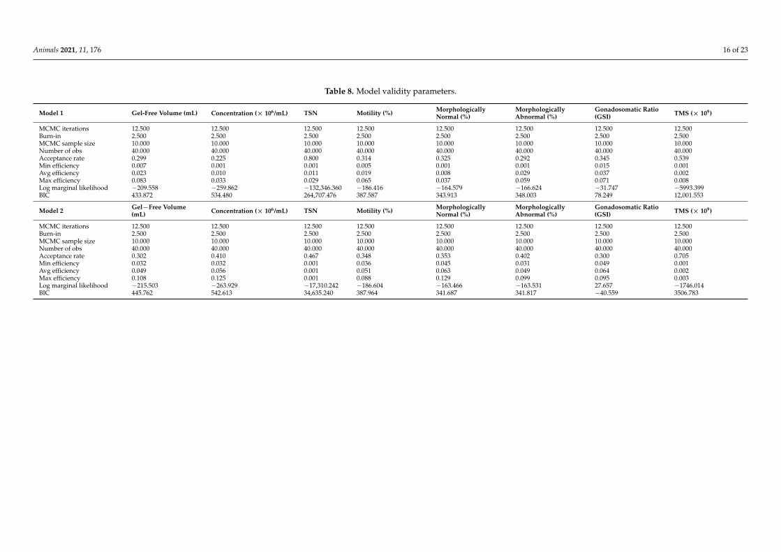
Yet, the combination of predictors in M=model 2 evidenced a higher likelihood topredict for TSN (×109), morphologically normal and abnormal spermatozoa (%), TMS(×109) and gonadosomatic ratio (GSI) (%), (BIC: −40.559 to 34,635.240). Age-related effectswere verified on the following parameters: gel-free volume, morphologically abnormalspermatozoa (%), and TSN (Tables 5 and 6). The summary of the results for the parametersof validity of both models is reported in Table 8.

Animals 2021, 11, 176 14 of 23

Table 5. Bayesian Estimates of Unstandardized Linear Regression Coefficients for predictive model 1 for gel-free volume (mL), concentration (×106/mL), morphologically normal (%), andmorphologically abnormal (%) sperm output in Miranda donkey breed.

Parameter Posterior 95% Credible Interval Parameter Posterior 95% Credible Interval

Gel-free volume (mL) Mean SD MCSE Lower Bound Upper Bound Morphologically normal (%) Mean SD MCSE Lower Bound Upper Bound

(Intercept) 6.750 85.650 7.882 11.940 −159.039 (Intercept) 38.820 61.999 17.656 35.535 −69.634Age (months) 0.554 0.186 0.020 0.551 0.190 Age (months) 0.009 0.120 0.033 0.016 −0.273

Length LT (cm) −7.618 23.395 2.210 −8.748 −52.776 Length LT (cm) 7.176 15.183 4.290 8.154 −29.472Length RT (cm) −8.047 19.952 1.350 −7.762 −45.424 Length RT (cm) −7.758 6.349 0.756 −7.367 −21.025Height LT (cm) 39.055 10.577 0.513 39.257 16.789 Height LT (cm) 4.253 2.752 0.142 4.226 −1.076Height RT (cm) −0.142 15.488 1.598 −0.446 −30.291 Height RT (cm) −2.344 10.261 2.868 −3.001 −20.264Width LT (cm) −8.293 13.214 1.203 −8.355 −35.057 Width LT (cm) 2.925 5.712 1.243 3.167 −7.979Width RT (cm) −0.867 16.024 1.877 −0.780 −32.031 Width RT (cm) 3.021 6.681 1.586 2.709 −10.081

Concentration (×106/mL) Mean SD MCSE Lower Bound Upper Bound Morphologically abnormal (%) Mean SD MCSE Lower Bound Upper Bound

(Intercept) 119.325 95.837 6.792 120.692 −67.802 (Intercept) −92.566 4.923 1.290 −92.168 −102.543Age (months) −1.675 0.438 0.024 −1.672 −2.510 Age (months) 0.268 0.036 0.002 0.267 0.199

Length LT (cm) −179.851 51.735 14.252 −170.219 −289.282 Length LT (cm) 28.736 4.098 0.370 28.543 21.311Length RT (cm) 112.455 63.065 7.805 114.114 −13.492 Length RT (cm) 1.078 5.696 0.306 1.182 −10.506Height LT (cm) −82.447 38.657 3.239 −84.282 −154.495 Height LT (cm) −5.022 2.742 0.145 −5.009 −10.399Height RT (cm) 60.562 33.694 8.149 57.459 2.457 Height RT (cm) −22.037 2.535 0.272 −21.978 −27.089Width LT (cm) 143.483 47.524 9.710 138.746 58.199 Width LT (cm) 8.980 3.366 0.145 8.888 2.389Width RT (cm) 12.984 51.340 8.872 9.472 −80.658 Width RT (cm) −15.696 3.963 0.276 −15.608 −23.572

LT—left testicle; RT—right testicle.

Table 6. Bayesian Estimates of Unstandardized Linear Regression Coefficients for predictive model 1 for TSN, gonadosomatic ratio (GSI) (%), motility (%), and TMS (×109) sperm outputin Miranda donkey breed.

Parameter Posterior 95% Credible Interval Parameter Posterior 95% Credible Interval

TSN Mean SD MCSE Lower Bound Upper Bound Gonadosomatic ratio (GSI) Mean SD MCSE Lower Bound Upper Bound

(Intercept) 23,753.340 80.646 4.744 23,753.840 23,598.750 (Intercept) −0.600 0.035 0.003 −0.602 −0.670Age (months) −1416.025 443.100 133.800 −1451.571 −2085.682 Age (months) 0.000 0.000 0.000 0.000 −0.001

Length LT (cm) 8883.943 111.914 30.604 8885.097 8667.620 Length LT (cm) 0.048 0.031 0.003 0.046 −0.014Length RT (cm) 13,450.930 78.239 21.894 13,444.170 13,319.860 Length RT (cm) −0.086 0.036 0.004 −0.086 −0.156Height LT (cm) −33,418.180 131.843 37.637 −33,411.060 −33,681.770 Height LT (cm) 0.154 0.029 0.003 0.153 0.099Height RT (cm) 3060.495 62.605 4.230 3059.644 2940.727 Height RT (cm) 0.097 0.027 0.002 0.097 0.046Width LT (cm) 19,157.550 69.930 5.174 19,157.660 19,020.890 Width LT (cm) 0.036 0.030 0.003 0.037 −0.034Width RT (cm) −17,716.000 24.807 1.749 −17,716.020 −17,763.690 Width RT (cm) 0.072 0.025 0.002 0.071 0.026

Motility (%) Mean SD MCSE Lower Bound Upper Bound TMS (× 109) Mean SD MCSE Lower Bound Upper Bound

(Intercept) −12.707 90.778 13.158 −11.443 −185.472 (Intercept) −782.074 1094.008 328.918 −1260.849 −1857.071Age (months) −0.069 0.175 0.022 −0.070 −0.390 Age (months) −612.420 250.955 74.637 −643.819 −958.823

Length LT (cm) 16.644 21.823 3.203 15.668 −24.687 Length LT (cm) −3816.467 87.995 16.210 −3819.298 −3982.185Length RT (cm) 12.235 11.157 0.668 11.796 −9.577 Length RT (cm) 4859.292 206.757 60.216 4806.093 4601.664Height LT (cm) −5.247 5.292 0.369 −5.314 −15.183 Height LT (cm) −2809.112 2318.070 702.958 −1870.947 −7896.015Height RT (cm) −11.939 14.762 2.118 −11.310 −40.592 Height RT (cm) 536.574 140.014 15.828 524.424 295.207Width LT (cm) 2.605 9.550 0.603 2.700 −16.521 Width LT (cm) 1678.912 2687.695 816.107 484.096 −742.483Width RT (cm) −13.494 10.278 0.916 −13.619 −33.146 Width RT (cm) −7924.881 837.695 252.844 −7632.309 −9824.660

Animals 2021, 11, 176 15 of 23

Table 7. Bayesian Estimates of Unstandardized Linear Regression Coefficients for predictive model 2 for gel-free volume (mL), concentration (×106/mL), morphologically normal (%) andmorphologically abnormal (%), TSN, gonadosomatic ratio (GSI) (%), motility (%), and TMS (×109) sperm output in Miranda donkey breed.

Parameter Posterior 95% Credible Interval Parameter Posterior 95% Credible Interval

Gel-free volume (mL) Mean SD MCSE Lower Bound Upper Bound Morphologically normal (%) Mean SD MCSE Lower Bound Upper Bound

(Intercept) 18.027 74.948 4.027 17.645 −131.021 (Intercept) 101.165 48.993 2.230 102.862 6.593Age (months) 0.380 0.075 0.003 0.386 0.228 Age (months) −0.088 0.028 0.001 −0.089 −0.141

BW (kg) 0.059 0.241 0.013 0.057 −0.408 BW (kg) −0.048 0.153 0.007 −0.051 −0.353TTV (cm3) 0.229 0.206 0.011 0.237 −0.183 TTV (cm3) 0.082 0.130 0.006 0.086 −0.178

GSI −61.537 63.042 3.287 −61.751 −178.796 GSI −16.479 39.912 1.736 −17.993 −95.823

Concentration(× 106/mL) Mean SD MCSE Lower Bound Upper Bound Morphologically abnormal (%) Mean SD MCSE Lower Bound Upper Bound

(Intercept) 34.599 87.218 4.216 29.855 −135.220 (Intercept) −34.631 48.161 2.471 −33.664 −130.104Age (months) −1.281 0.246 0.012 −1.287 −1.751 Age (months) 0.098 0.027 0.002 0.098 0.045

BW (kg) 1.577 0.397 0.018 1.568 0.802 BW (kg) 0.151 0.151 0.008 0.147 −0.133TTV (cm3) −0.434 0.282 0.013 −0.443 −1.002 TTV (cm3) −0.167 0.128 0.006 −0.168 −0.424

GSI 71.418 77.349 4.329 72.597 −84.034 GSI 43.228 39.364 1.902 43.112 −30.970

TSN Mean SD MCSE Lower Bound Upper Bound Gonadosomatic ratio (GSI) (%) Mean SD MCSE Lower Bound Upper Bound

(Intercept) 11,264.220 1978.212 598.275 10,786.800 8794.520 (Intercept) 1.213 0.036 0.001 1.214 1.140Age (months) 4577.180 417.008 125.933 4671.496 3705.060 Age (months) −0.001 0.000 0.000 −0.001 −0.001

BW (kg) −5091.494 439.681 133.092 −5203.422 −5634.810 BW (kg) −0.004 0.000 0.000 −0.004 −0.004TTV (cm3) 2606.332 220.725 66.742 2662.469 2131.406

TTV (cm3) 0.003 0.000 0.000 0.003 0.003GSI −4379.107 756.935 227.540 −4209.127 −5956.150

Motility (%) Mean SD MCSE Lower Bound Upper Bound TMS (× 109) Mean SD MCSE Lower Bound Upper Bound

(Intercept) 10.199 65.301 3.019 8.928 −114.356 (Intercept) −4076.090 195.502 54.547 −4028.317 −4586.811Age (months) −0.116 0.043 0.002 −0.116 −0.202 Age (months) −1422.795 311.451 88.829 −1524.509 −1776.786

BW (kg) 0.223 0.206 0.010 0.221 −0.173 BW (kg) 569.508 82.412 14.404 572.642 397.312TTV (cm3) −0.152 0.175 0.008 −0.156 −0.484 TTV (cm3) −172.885 46.034 7.844 −172.536 −261.502

GSI 51.775 53.600 2.428 54.210 −54.645 GSI 2298.200 133.412 29.547 2281.863 2070.603

TTV—total testicular volume; TSN—total sperm number; TMS—total motile sperm count; GSI—gonadosomatic ratio.

Animals 2021, 11, 176 16 of 23

Table 8. Model validity parameters.

Model 1 Gel-Free Volume (mL) Concentration (× 106/mL) TSN Motility (%) MorphologicallyNormal (%)

MorphologicallyAbnormal (%)

Gonadosomatic Ratio(GSI) TMS (× 109)

MCMC iterations 12.500 12.500 12.500 12.500 12.500 12.500 12.500 12.500Burn-in 2.500 2.500 2.500 2.500 2.500 2.500 2.500 2.500MCMC sample size 10.000 10.000 10.000 10.000 10.000 10.000 10.000 10.000Number of obs 40.000 40.000 40.000 40.000 40.000 40.000 40.000 40.000Acceptance rate 0.299 0.225 0.800 0.314 0.325 0.292 0.345 0.539Min efficiency 0.007 0.001 0.001 0.005 0.001 0.001 0.015 0.001Avg efficiency 0.023 0.010 0.011 0.019 0.008 0.029 0.037 0.002Max efficiency 0.083 0.033 0.029 0.065 0.037 0.059 0.071 0.008Log marginal likelihood −209.558 −259.862 −132,346.360 −186.416 −164.579 −166.624 −31.747 −5993.399BIC 433.872 534.480 264,707.476 387.587 343.913 348.003 78.249 12,001.553

Model 2 Gel−Free Volume(mL) Concentration (× 106/mL) TSN Motility (%) Morphologically

Normal (%)MorphologicallyAbnormal (%)

Gonadosomatic Ratio(GSI) TMS (× 109)

MCMC iterations 12.500 12.500 12.500 12.500 12.500 12.500 12.500 12.500Burn-in 2.500 2.500 2.500 2.500 2.500 2.500 2.500 2.500MCMC sample size 10.000 10.000 10.000 10.000 10.000 10.000 10.000 10.000Number of obs 40.000 40.000 40.000 40.000 40.000 40.000 40.000 40.000Acceptance rate 0.302 0.410 0.467 0.348 0.353 0.402 0.300 0.705Min efficiency 0.032 0.032 0.001 0.036 0.045 0.031 0.049 0.001Avg efficiency 0.049 0.056 0.001 0.051 0.063 0.049 0.064 0.002Max efficiency 0.108 0.125 0.001 0.088 0.129 0.099 0.095 0.003Log marginal likelihood −215.503 −263.929 −17,310.242 −186.604 −163.466 −163.531 27.657 −1746.014BIC 445.762 542.613 34,635.240 387.964 341.687 341.817 −40.559 3506.783

Animals 2021, 11, 176 17 of 23

4. Discussion4.1. Testicular Morphometry (Juveniles and Matures) and Sperm Quality Parameters in MirandaDonkey Breed

The indication that testis biometry could provide a quantitative indication of spermproduction has been previously reported in bulls [55,56], bucks [57,58], and dogs [59,60]. Inthe horse, morphometric, ultrasonographic-echotextural, and histomorphometric studieshave been carried out [3,59,60], which evidenced the relation between testicular dimensionsand sperm outputs [2] and the contribution of the ultrasonographic (US) evaluation in theaccurate evaluation of the testicular functional status [61].

Albeit less than in horses, some studies on testicular morphometry have been con-ducted in donkey breeds such as Brazilian Pêga [6,62]; Ethiopian [63]; Egyptian [64,65];and in the Italian breeds, Ragusano [19] and Martina Franca [66,67]. These studies haveaddressed the considerable existing variation among donkey breeds, which led to the needof investigating testicular dimensions in Miranda donkey breed. Besides, no previousworks on Bayesian approaches to predict for sperm output and quality in donkeys hasbeen conducted to the knowledge of the authors.

Mean US values of TTV of 271.69 cm3 (±133.21) obtained in mature Miranda donkeyswere higher than those found in Egyptian donkeys [64], similar to those in Brazilian Pêgadonkeys [62], and lower than those reported for Ethiopian donkeys [63]. In comparisonto other morphologically similar breeds to Miranda donkey, our values were similar toslightly lower than TTV values found in Ragusano and Martina Franca donkeys [19,66].Even if all the aforementioned breeds were medium to large-sized, differences of TTVcould still be attributed to BW, age and management conditions of the males selected forthe studies.

In the juveniles, studies are still scarce, but the values in our study (17.74 ± 9.89 cm3)were similar to those described for the prepubertal Egyptian [68] and Amiata donkeys [67].Donkeys between 10 to 14 months are still in their pubertal transition period and, whichreaches its end at 19–20 months of age, when testis have presumably completed theirdescent into the scrotum [37]. In the present work, a rapid increment of TV was verifiedafter 11–12 months, which, besides, was simultaneous to the increase of BW. Accordingto the work by Rota, et al. [67], a progressive increase of testicular width was noted after10 months, and notably after 16 months of age; however, puberty—defined by the firstpresence in the ejaculate of 50×106 sperm with at least 10% of motility-, was not attained indonkeys before 19–20 months. A previous histological work by our group evidenced thatalthough a rapid increase of TV could be observed after 12–14 months, spermatogenesiswas still incipient at that age [69]. Still, further studies should be carried out to preciselydetermine the age of Miranda donkey at puberty.

The comparative analysis of US measurements with those obtained using a precisioncaliper after orchiectomy evidenced that the former were very accurate. The preciseposition and orientation of the probe during US examination and the correct handling ofthe testicle, avoiding excessive tension during the exam, may have additionally contributedto the obtention of reliable US measurements.

The quantitative and qualitative sperm parameters obtained; total sperm number(TSN) per ejaculate, volume, concentration and morphology were within the range foundfor other European Donkey breeds such as Zamorano–Leonese [70], Catalonian [71], An-dalusian [72–74], and Amiata donkey [67]. The values of GSI obtained for mature donkeys(0.9494) were higher than those reported in other domestic species [5]. This finding is ofgreat interest and application when implementing ARTs’ strategies and is consistent withprevious studies that observed the comparatively greater efficiency for sperm productionof donkeys among mammals, characterizing by a high spermatogenic efficiency and shortlength of spermatogenesis [6,75].

Animals 2021, 11, 176 18 of 23

4.2. Bayesian Approach and Predictive Models

Comparative observations were taken at different time points, from a populationwhose membership changes over time, but retains some constant members. This samplecondition is known as partially overlapping samples and for this study, it implies thefact that not all the animals which were measured for morphometric parameters wereevaluated for semen parameters. As reported by Kay, et al. [76] in studies working withpartially overlapping samples, when there has been a gross violation of normality, as in ourstudy, samples should be considered independent. In a nonparametric context, the strongsubdivision of samples across the different experiments may condition results, hence, aBayesian approach was followed given smaller data sets that can be evaluated avoidingpower loss and retaining precision.

Posterior predictive p values (total model probability) for models 1 and 2 of around0.331. Indicated moderately plausible good-fitting models. Similarly, the difference of morethan 3 log likelihood units can be considered as strong evidence against models 1 or 2depending on the parameters considered. The higher value reported for this parametermay suggest the acceptance of a more parameter-rich or simpler model accordingly. BICexplains how well the model will fit for new data (instead of explaining the existing data,which is measured by Adjusted R2). Models presenting lower BIC values evidence im-proved predictions for the dependent variable or variables that they model for. Frequently,adding more variables decreases predictive accuracy, and in that case, the model with evenhigher Adjusted R2 will display higher BIC, decreasing its predictive power [52,76,77].However, considering the higher Adjusted R2 and the lower BIC, model 1 performs betterat explaining and predicting than model 2 for gel-free volume (mL) and concentration(×106/mL). For motility (%), model 1 was more precise to predict for future data whileslightly worse at explaining present data (0.01 lower R2). The opposite situation wasreported for TSN (×109) and TMS (×109), for which model 2 was more precise to predictfor future data, although it may be slightly worse at explaining present data (0.13 lower R2).For morphologically normal and abnormal spermatozoa (%) and gonadosomatic ratio (GSI)(%), model 2 suggested a higher ability to explain for present and predict for future data.

In the present research, when comparatively analyzing testis’ biometry predictivepower on spermatic parameters, some differences were found. The left testicle seems toexert a higher influence on gel-free volume, while, on the other hand, the biometry of thetesticles seems to affect TSN differently. Concretely, the length and width of the left testicleand the height of the right testicle seem to increase in parallel with sperm quantitativeparameters. Oppositely, as length and width of right testicle and height of the left testicleincrease, sperms output parameters seem to decrease. Hence, the negative/positive balancebetween linear regression coefficients of morphometry variables (length, width and height)suggest that testis may reciprocally react to changes in the contralateral testicle, whichaffects almost all sperm outputs variables.

A previous work purposes the “compensation hypothesis” in birds, that states thatone of the testis could serve as a “back-up” for any reduced function of the other andprovides a mechanism to explain intraspecific variation in degree and direction of go-nad asymmetry [77]. Another work relates that the degree of testicular asymmetry waspositively correlated with inbreeding coefficient and negatively correlated with the pro-portion of normal sperm [78]. However, in the present work, testicular asymmetry wasnot found in both clinical and morphometric evaluation, as both features do not meet theinclusion criterion.

Mahmoud Ali Omar, et al. [79] reported a similar compensatory effect in the right tes-ticle after the removal of the contralateral testicle in donkeys. Other authors have ascribedthis compensation to the increase in serum LH and FSH concentrations and, potentiallyhigher intratesticular testosterone [80]. Unilateral orchiectomy has been reported to in-crease the mean diameter of seminiferous tubules by 21% and of their lumina by 51% [81].Additionally, two events in line with our results were described. A weight compensationwas reported for the remaining testis, which has been already described [82]. Also, the

Animals 2021, 11, 176 19 of 23

histological examination of the testis of donkeys after unilateral orchiectomy with scrotumsuture revealed hyperplasia of Leydig and Sertoli cells [79]. This had also been reported byPutra and Blackshaw [83], who suggested an increase in the number of Sertoli cells andgerm cells occupying the seminiferous epithelium after unilateral orchiectomy. Our resultsmay evidence that compensation may occur physiologically without these events, as ithas also been reported in other species [78]. Still, future works are necessary in order toconfirm these findings in donkeys.

In the present study, the age covariate, included in both predictive models, wassignificantly and positively correlated with several parameters, namely with gel-freevolume and sperm output (TSN). The significant age-related positive effects on gel-freevolume and TSN agreed those in previous works in stallions [84,85]. For instance, theinfluence of age in testicular dimensions of juvenile and peripubertal donkeys was verifiedby Rota, et al. [67], who suggested that age markedly influenced testicular width.

On the other hand, age shows a linear association with abnormal sperm morphologyin model 1. Morphologically abnormal spermatozoa percentage slightly increases with age;while sperm concentration and morphologically normal spermatozoa linearly decrease.The negative impact of advanced age on morphology has been already described in stallionsand has been ascribed to testicular degeneration, abnormal epididymal function [86] or toage-related testicular dysfunction associated with deterioration in DNA sperm motility [87].A study in Egyptian donkeys reports that from six years onward, histological features wereindicative of spermatogenic efficiency starting to decrease [65]; however, more studiesshould be performed before concluding that the same occurs in Miranda donkey breed.

In general, stronger correlations between BW and testicular biometry than betweenage and testicular biometry were verified in the present study. This agrees with thefindings in a previous study conducted in stallions which emphasized the influence ofbody size in testicular measurements and sperm output [2]. However, the analysis ofregression coefficients evidenced that the association of motility and total motile sperm(TMS) with TTV was not always constant. On the contrary, sperm motility, as well as TMSand concentration, were positively and linearly associated with gonodasomatic ratio (GSI).Overall, this supports the fact that even if the measurements of the testicular parameterscould provide useful information about the potential sperm production, when it comes topredict motility, these parameters should be adjusted for the BW of the donkey, as reportedby [Woodall and Johnstone [88]] when predicting for fertility in dogs. Contextually, furtherinvestigations should allow to determine and confirm the relationship between BW andTV in donkeys.

5. Conclusions

The results of the present work evidence the reliability of ultrasonographic measure-ments of testis, which emphasizes its importance and value to obtain reference values ofdonkey testicular volumes. Values of testicular volume and sperm output in the Mirandadonkey breed are similar to those in other affine European donkey breeds. Gonadomaticindex (GSI) is higher in the donkey than in other domestic species as previously described,which confirms the great reproductive potential of male donkeys.

Combinations of biometrical and testicular morphometric factors (age, body weight,testicular volume and GSI) will likely improve the predictive accuracy of Models thanusing factors separately. Besides biometry, considering data such as BW and age, testicularvolume, and GSI may be systematically taken into consideration and integrated on BSEof donkeys. The present study provides new insights into donkey reproductive biology,which may be transferred to ARS strategies. Appropriate use of both models may be usefulto further improve knowledge on the reproductive characteristics of donkey breeds, whichmay reinforce clinical purposes and maximize the outcomes from direct conservation orselection strategies.

Animals 2021, 11, 176 20 of 23

Supplementary Materials: The following Tables are available online at https://www.mdpi.com/2076-2615/11/1/176/s1, Table S1. Testing for normality using Shapiro–Francia W’ test (for 50 < n <2500 samples) for testicular biometry.; Table S2. Testing for normality using Shapiro–Wilk test (for n <50 samples) for testicular biometry (n = 16 testis) and spermatic data (n = 40 ejaculates) of eight maturedonkeys.; Table S3. Bayesian Inference Pearson’s Correlation Coefficient function output summaryfor US and caliper testicle biometry.; Table S4. Commonly used thresholds to define significance ofevidence through Bayes factor (BF).; Table S5. Model validity and accuracy parameters definitionand interpretation.; Table S6. Descriptive statistic for US testicular in six juveniles and 17 maturesdonkeys (n = 46 testis) and caliper meas-urements after orchiectomy in seven of these donkeys (n =14 testis).; Table S7a. Posterior distribution statistics for US and caliper testicular measurements injuvenile (n = 6) and mature donkeys (n = 17).; Table S7b. Summary of Bayesian ANOVA outputs totest for differences in the mean for US and caliper testicular measurements between juvenile (n = 6)and mature donkeys (n = 17).

Author Contributions: Conceptualization, A.M.-B. and F.J.N.G.; methodology, A.M.-B. and F.J.N.G.;software, F.J.N.G.; validation, A.M.-B., M.Q., and A.C.; formal analysis, F.J.N.G.; investigation, A.M.-B.and M.Q.; resources, M.Q., B.L., A.C., and A.M.-B.; data curation, F.J.N.G.; writing—original draftpreparation, A.M.-B., M.Q., and A.C.; writing—review and editing, A.M.-B. and F.J.N.G.; visualiza-tion, A.M.-B. and F.J.N.G.; supervision, A.M.-B.; project administration, A.M.-B.; funding acquisition,A.M.-B. and M.Q. All authors have read and agreed to the published version of the manuscript.

Funding: This work was supported by the project UIDB/CVT/00772/2020 funded by the supportedby the Portuguese Science and Technology Foundation (FCT).

Institutional Review Board Statement: The study was conducted in accordance with the Declarationof Helsinki. Animals have been evaluated with approval and in collaboration with the Associationfor Study and Protection of the Donkey Breed Burro de Miranda (AEPGA), in the behalf of a scientificprotocol of caooperation signed between both institutions. All animal procedures were conductedin accordance with national laws for animal welfare and experimentation as with the EU Directive2010/63/EU for animal experiments and the approval of the Directive Hospital Committee (ApprovalRef. 408/VTH-UTAD).

Informed Consent Statement: Not applicable.

Data Availability Statement: Data available on request due to restrictions eg privacy or ethical.

Acknowledgments: The authors thank the Veterinary Degree’ students for their willingness to partic-ipate in the present study. Also, the authors would like to thank the support of AEPGA-Associationfor the Study and Protection of Donkeys (Miranda do Douro, Portugal) and the Veterinary TeachingHospital of UTAD (Vila Real, Portugal) to carry out the present work. Critical comments from A.Rocha (DACT) and T. Guimarães (DECAR) (ICBAS and CRAV, University of Oporto, Portugal) arealso highly appreciated.

Conflicts of Interest: The authors declare no conflict of interest.

References1. Thompson, D.L., Jr.; Pickett, B.W.; Squires, E.L.; Amann, R.P. Testicular measurements and reproductive characteristics in stallions.

J. Reprod. Fertil. Suppl. 1979, 27, 13–17.2. Kavak, A.; Lundeheim, N.; Aidnik, M.; Einarsson, S. Testicular measurements and daily sperm output of Tori and Estonian breed

stallions. Reprod. Domest. Anim. 2003, 38, 167–169.3. Pricking, S.; Bollwein, H.; Spilker, K.; Martinsson, G.; Schweizer, A.; Thomas, S.; Oldenhof, H.; Sieme, H. Testicular volumetry

and prediction of daily sperm output in stallions by orchidometry and two-and three-dimensional sonography. Theriogenology2017, 104, 149–155. [PubMed]

4. Love, C. How to measure testes size and evaluate scrotal contents in the stallion. In Proceedings of the 60th AAEP AnnualConvention, Salt Lake City, UT, USA, 6–10 December 2014; Volume 60, pp. 302–308.

5. Lara, N.L.; Costa, G.M.; Avelar, G.F.; Lacerda, S.; Hess, R.A.; França, L.R. Testis physiology—overview and histology. InEncyclopedia of Reproduction; Skinner, M.K., Ed.; Academic Press: New York, NY, USA, 2018; pp. 105–116.

6. Neves, E.S.; Chiarini-Garcia, H.; França, L.R. Comparative testis morphometry and seminiferous epithelium cycle length indonkeys and mules. Biol. Reprod. 2002, 67, 247–255.

7. Kugler, W.; Grunenfelder, H.P.; Broxham, E. Donkey Breeds in Europe: Inventory, Description, Need for Action, Conservation; Report2007/2008; Monitoring Institute for Rare Breeds and Seeds in Europe: St. Gallen, Switzerland, 2008; p. 26.

Animals 2021, 11, 176 21 of 23

8. Quaresma, M.; Payan-Carreira, R. Characterization of the estrous cycle of Asinina de Miranda jennies (Equus asinus). Theriogenology2015, 83, 616–624. [PubMed]

9. Oravecz, Z.; Muth, C. Fitting growth curve models in the Bayesian framework. Psychon. Bull. Rev. 2018, 25, 235–255. [CrossRef][PubMed]

10. Knecht, D.; Jankowska-Makosa, A.; Duzinski, K. Boar genotype as a factor shaping age-related changes in semen parameters andreproduction longevity simulations. Theriogenology 2017, 98, 50–56. [PubMed]

11. Hox, J.; Moerbeek, M.; Kluytmans, A.; Van De Schoot, R. Analyzing indirect effects in cluster randomized trials. The effect ofestimation method, number of groups and group sizes on accuracy and power. Front. Psychol. 2014, 5, 78. [PubMed]

12. Lee, S.-Y.; Song, X.-Y. Evaluation of the Bayesian and maximum likelihood approaches in analyzing structural equation modelswith small sample sizes. Multivar. Behav. Res. 2004, 39, 653–686.

13. Peto, R.; Pike, M.; Armitage, P.; Breslow, N.; Cox, D.; Howard, S.V.; Mantel, N.; McPherson, K.; Peto, J.; Smith, P. Design andanalysis of randomized clinical trials requiring prolonged observation of each patient. I. Introduction and design. Br. J. Cancer1976, 34, 585–612.

14. Button, K.S.; Ioannidis, J.P.; Mokrysz, C.; Nosek, B.A.; Flint, J.; Robinson, E.S.; Munafò, M.R. Power failure: Why small samplesize undermines the reliability of neuroscience. Nat. Rev. Neurosci. 2013, 14, 365–376. [PubMed]

15. Stoltzfus, J.C. Logistic Regression: A Brief Primer. Acad. Emerg. Med. 2011, 18, 1099–1104. [CrossRef] [PubMed]16. Chen, Y.; Li, Y.; Wu, H.; Liang, L. Data envelopment analysis with missing data: A multiple linear regression analysis approach.

Int. J. Inf. Tech. Decis. 2014, 13, 137–153. [CrossRef]17. Navas, F.J.; Jordana, J.; León, J.M.; Barba, C.; Delgado, J.V. A model to infer the demographic structure evolution of endangered

donkey populations. Animal 2017, 11, 2129–2138. [CrossRef]18. Johnson, L.; Neaves, W.B. Age-related changes in the Leydig cell population, seminiferous tubules, and sperm production in

stallions. Biol. Reprod. 1981, 24, 703–712.19. Quartuccio, M.; Marino, G.; Zanghì, A.; Garufi, G.; Cristarella, S. Testicular volume and daily sperm output in Ragusano donkeys.

J. Equine Vet. Sci. 2011, 31, 143–146. [CrossRef]20. Kenney, R.M. Society for Theriogenology Manual for Clinical Evaluation of the Stallion; The Society for Theriogenology: Montgomery,

AL, USA, 1983.21. StataCorp. Stata Statistical Software, 15; StataCorp: College Station, TX, USA, 2017.22. IBM Corp. IBM SPSS Statistics for Windows, 25th ed.; IBM Corp: Armonk, NY, USA, 2017.23. Bakdash, J.Z.; Marusich, L.R. Repeated Measures Correlation. Front. Psychol. 2017, 8, 456. [CrossRef] [PubMed]24. IBM Corp. IBM SPSS Statistics Algorithms, 25th ed.; IBM Corp: Armonk, NY, USA, 2017; p. 110.25. Profillidis, V.A.; Botzoris, G.N. Chapter 5—Statistical Methods for Transport Demand Modeling. In Modeling of Transport Demand;

Profillidis, V.A., Botzoris, G.N., Eds.; Elsevier: Amsterdam, The Netherlands, 2019.26. Dogan, N.Ö. Bland-Altman analysis: A paradigm to understand correlation and agreement. Turk. J. Emerg. Med. 2018, 18, 139–141.

[CrossRef]27. Batterham, A.M. Bias in Bland-Altman but not Regression Validity Analyses. Sportscience 2004, 8, 42–47.28. Gelman, A.; Carlin, J.; Stern, H.; Rubin, D.; Dunson, D.; Vehtari, A. Solutions to some exercises from Bayesian Data Analysis, by

Gelman, Carlin, Stern, and Rubin. In Bayesian Data Analysis; Columbia University: New York, NY, USA, 2020.29. Brewer, K.R. Combined Survey Sampling Inference: Weighing Basu’s Elephants; Oxford University Press: Oxford, UK, 2002.30. Hayes, A.F.; Glynn, C.J.; Huge, M.E. Cautions Regarding the Interpretation of Regression Coefficients and Hypothesis Tests in

Linear Models with Interactions. Commun. Methods Meas. 2012, 6, 1–11.31. Liang, F.; Paulo, R.; Molina, G.; Clyde, M.A.; Berger, J.O. Mixtures of g priors for Bayesian variable selection. J. Am. Stat. Assoc.

2008, 103, 410–423. [CrossRef]32. Heck, D. A Caveat on the Savage-Dickey Density Ratio: The Case of Computing Bayes Factors for Regression Parameters. Br. J.

Math. Stat. Psychol. 2019, 72, 316–333. [CrossRef] [PubMed]33. Zellner, A.; Siow, A. Posterior odds ratios for selected regression hypotheses. Trab. Estadística Y Investig. Oper. 1980, 31, 585–603.

[CrossRef]34. Rouder, J.N.; Morey, R.D.; Speckman, P.L.; Province, J.M. Default Bayes factors for ANOVA designs. J. Math. Psychol. 2012, 56,

356–374. [CrossRef]35. Bayarri, M.J.; Berger, J.O.; Forte, A.; García-Donato, G. Criteria for Bayesian model choice with application to variable selection.

Ann. Stat. 2012, 40, 1550–1577. [CrossRef]36. Rouder, J.N.; Morey, R.D. Default Bayes factors for model selection in regression. Multivar. Behav. Res. 2012, 47, 877–903.

[CrossRef] [PubMed]37. Morey, R.; Rouder, J. BayesFactor 0.9. 12-2; Comprehensive R Archive Network: Vienna, Austria, 2015.38. Rouder, J.N.; Speckman, P.L.; Sun, D.; Morey, R.D.; Iverson, G. Bayesian t tests for accepting and rejecting the null hypothesis.

Psychon. Bull. Rev. 2009, 16, 225–237. [CrossRef] [PubMed]39. Depaoli, S.; Van de Schoot, R. Improving transparency and replication in Bayesian statistics: The WAMBS-Checklist. Psychol.

Methods 2017, 22, 240. [CrossRef]40. Kass, R.E.; Raftery, A.E. Bayes factors. J. Am. Stat. Assoc. 1995, 90, 773–795. [CrossRef]

Animals 2021, 11, 176 22 of 23

41. Arora, J.S. Chapter 14—Practical Applications of Optimization. In Introduction to Optimum Design, 4th ed.; Arora, J.S., Ed.;Academic Press: Boston, MA, USA, 2017; pp. 601–680.

42. Pizarro Inostroza, M.G.; Navas González, F.J.; Landi, V.; León Jurado, J.M.; Delgado Bermejo, J.V.; Fernández Álvarez, J.;Martínez Martínez, M.D.A. Bayesian Analysis of the Association between Casein Complex Haplotype Variants and Milk Yield,Composition, and Curve Shape Parameters in Murciano-Granadina Goats. Animals 2020, 10, 1845. [CrossRef]

43. Geweke, J. Variable selection and model comparison in regression. In Proceedings of the Fifth Valencia International Meeting,Valencia, Spain, 5–9 June 1994.

44. Analla, M. Model validation through the linear regression fit to actual versus predicted values. Agric. Syst. 1998, 57, 115–119.[CrossRef]

45. Pizarro Inostroza, M.G.; Navas González, F.J.; Landi, V.; León Jurado, J.M.; Delgado Bermejo, J.V.; Fernández Álvarez, J.;Martínez Martínez, M.D.A. Software-Automatized Individual Lactation Model Fitting, Peak and Persistence and BayesianCriteria Comparison for Milk Yield Genetic Studies in Murciano-Granadina Goats. Mathematics 2020, 8, 1505. [CrossRef]

46. Pizarro Inostroza, M.G.; Navas González, F.J.; Landi, V.; León Jurado, J.M.; Delgado Bermejo, J.V.; Fernández Álvarez, J.; Martínez,M.D.A.M. Goat Milk Nutritional Quality Software-Automatized Individual Curve Model Fitting, Shape Parameters Calculationand Bayesian Flexibility Criteria Comparison. Animals 2020, 10, 1693. [CrossRef] [PubMed]

47. Hall, P.; Maiti, T. Nonparametric estimation of mean-squared prediction error in nested-error regression models. Ann. Stat. 2006,34, 1733–1750. [CrossRef]

48. Jeffreys, H. Theory of Probability, 3rd ed.; Oxford University Press: Oxford, UK, 1961.49. Lee, M.; Wagenmakers, E. Bayesian Data Analysis for Cognitive Science: A Practical Course; Cambridge University Press: New York,

NY, USA, 2013.50. Kaplan, D.; Depaoli, S. Bayesian structural equation modeling. In Handbook of Structural Equation Modeling; Hoyle, H., Ed.; The

Guilford Press: New York, NY, USA; pp. 650–673.51. Gelman, A.; Carlin, J.B.; Stern, H.S.; Dunson, D.B.; Vehtari, A.; Rubin, D.B. Bayesian Data Analysis; CRC Press: Boca Ratón, FL,

USA, 2013.52. Drton, M.; Plummer, M. A Bayesian information criterion for singular models. J. R. Stat. Soc. B 2017, 79, 323–380. [CrossRef]53. Clyde, M.; Cetinkaya-Rundel, M.; Rundel, C.; Banks, D.; Chai, C.; Huang, L. Bayesian Model Choice. In An Introduction to Bayesian

Thinking: A Companion to the Statistics with R Course; Clyde, M., Cetinkaya-Rundel, M., Rundel, C., Banks, D., Chai, C., Huang, L., Eds.;Coursera: Mountain View, CA, USA, 2019; Chapter 7.

54. Gelman, A.; Goodrich, B.; Gabry, J.; Vehtari, A. R-squared for Bayesian regression models. Am. Stat. 2019, 73, 307–309. [CrossRef]55. Kumar, S.; Srivastava, S. Testicular biometry and its correlation with body weight and semen output in murrah bull. Buffalo Bull.

2017, 36, 105–114.56. Brito, L.F.; Silva, A.E.; Barbosa, R.T.; Kastelic, J.P. Testicular thermoregulation in Bos indicus, crossbred and Bos taurus bulls:

Relationship with scrotal, testicular vascular cone and testicular morphology, and effects on semen quality and sperm production.Theriogenology 2004, 61, 511–528. [CrossRef]

57. Gemeda, A.E.; Workalemahu, K. Body weight and scrotal-testicular biometry in three indigenous breeds of bucks in arid andsemiarid agroecologies, Ethiopia. J. Vet. Med. 2017, 2017. [CrossRef]

58. Kerketta, S.; Singh, M.; Patel, B.; Dutt, T.; Upadhyay, D.; Bharti, P.; Sahu, S.; Kamal, R. Relationships between age, bodymeasurements, testicular measurements and total ejaculation of semen in local goat of Rohilkhand region. Small Rum. Res. 2015,130, 193–196. [CrossRef]

59. Olar, T.; Amann, R.; Pickett, B. Relationships among testicular size, daily production and output of spermatozoa, and extragonadalspermatozoal reserves of the dog. Biol. Reprod. 1983, 29, 1114–1120. [CrossRef] [PubMed]

60. Mialot, J.; Guerin, C.; Begon, D. Growth, testicular development and sperm output in the dog from birth to post pubertal period.Andrologia 1985, 17, 450–460. [CrossRef] [PubMed]

61. Pozor, M.; Morrissey, H.; Albanese, V.; Khouzam, N.; Deriberprey, A.; Macpherson, M.L.; Kelleman, A.A. Relationship betweenechotextural and histomorphometric characteristics of stallion testes. Theriogenology 2017, 99, 134–145. [CrossRef] [PubMed]

62. Canisso, I.F.; Morel, M.D.; McDonnell, S. Strategies for the management of donkey jacks in intensive breeding systems. Equine Vet.Educ. 2009, 21, 652–659. [CrossRef]

63. Lemma, A.; Deressa, B. Study on reproductive activity and evaluation of breeding soundness of jacks (Equus asinus) in andaround Debre Zeit, Ethiopia. Livest. Res. Rural. Dev. 2009, 21, 126.

64. Moustafa, M.; Sayed, R.; Zayed, A.; El-Hafeez, A.H. Morphological and morphometric study of the development of seminiferousepithelium of donkey (Equus asinus) from birth to maturity. J. Cytol. Histol. 2015, 6, 1.

65. Nipken, C.; Wrobel, K. A quantitative morphological study of age-related changes in the donkey testis in the period betweenpuberty and senium. Andrologia 1997, 29, 149–161. [CrossRef]

66. Carluccio, A.; Panzani, S.; Contri, A.; Bronzo, V.; Robbe, D.; Veronesi, M. Influence of season on testicular morphometry andsemen characteristics in Martina Franca jackasses. Theriogenology 2013, 79, 502–507. [CrossRef]

67. Rota, A.; Puddu, B.; Sabatini, C.; Panzani, D.; Lainé, A.-L.; Camillo, F. Reproductive parameters of donkey jacks undergoingpuberty. Anim. Reprod. Sci. 2018, 192, 119–125. [CrossRef]

68. Abdelhafeez, H.; Moustafa, M.; Zayed, A.; Sayed, R. Morphological and Morphometric Study of the Development of Leydig Cellpopulation of Donkey (Equus asinus) Testis from Birth to Maturity. Cell Biol. 2017, 6, 1. [CrossRef]

Animals 2021, 11, 176 23 of 23

69. Calado, A.; Lemos, H.; Leiva, B.; Quaresma, M.; Martins-Bessa, A. Comparative testicular histology from adult Equus Asinusand Equus Caballus. In Proceedings of the Book INCOMAM 18—52◦ International Congress on Microscopy and Microanalysis,Coimbra, Portugal, 12–13 October 2018; p. 35.

70. Serres, C. Evaluación y Conservación del Semen en el Asno Zamorano-Leonés. Ph.D. Thesis, Complutense University of Madrid,Madrid, Spain, 2003.

71. Miró, J.; Lobo, V.; Quintero-Moreno, A.; Medrano, A.; Peña, A.; Rigau, T. Sperm motility patterns and metabolism in Cataloniandonkey semen. Theriogenology 2005, 63, 1706–1716. [CrossRef] [PubMed]

72. Ortiz, I.; Dorado, J.; Ramírez, L.; Morrell, J.M.; Acha, D.; Urbano, M.; Gálvez, M.J.; Carrasco, J.J.; Gómez-Arrones, V.; Calero-Carretero, R.; et al. Effect of single layer centrifugation using Androcoll-E-Large on the sperm quality parameters of cooled-storeddonkey semen doses. Animal 2013, 8, 308–315. [CrossRef] [PubMed]

73. Dorado, J.; Acha, D.; Ortiz, I.; Gálvez, M.; Carrasco, J.; Díaz, B.; Gómez-Arrones, V.; Calero-Carretero, R.; Hidalgo, M. Relationshipbetween conventional semen characteristics, sperm motility patterns and fertility of Andalusian donkeys (Equus asinus). Anim.Reprod. Sci. 2013, 143, 64–71. [CrossRef] [PubMed]

74. Dorado, J.; Acha, D.; Ortiz, I.; Gálvez, M.; Carrasco, J.; Gómez-Arrones, V.; Calero-Carretero, R.; Hidalgo, M. Effect of extenderand amino acid supplementation on sperm quality of cooled-preserved Andalusian donkey (Equus asinus) spermatozoa. Anim.Reprod. Sci. 2014, 146, 79–88. [CrossRef]

75. Canisso, I.F.; Panzani, D.; Miró, J.; Ellerbrock, R.E. Key Aspects of Donkey and Mule Reproduction. Vet. Clin. Equine 2019, 35,607–642. [CrossRef]

76. Kay, G.; Tligui, N.; Semmate, N.; Azrib, R.; González, F.J.N.; Brizgys, L.; McLean, A. Determining factors and interspecificmodeling for serum amyloid a concentrations in working horses, donkeys, and mules. Res. Vet. Sci. 2019, 125, 256–265. [CrossRef]

77. Calhim, S.; Birkhead, T.R. Intraspecific variation in testis asymmetry in birds: Evidence for naturally occurring compensation.Proc. Biol. Sci. 2009, 276, 2279–2284. [CrossRef]

78. Cassinello, J.; Abaigar, T.; Gomendio, M.; Roldan, E. Characteristics of the semen of three endangered species of gazelles (Gazelladama mhorr, G. dorcas neglecta and G. cuvieri). Reproduction 1998, 113, 35–45. [CrossRef]

79. Omar, M.M.A.; Hassanein, K.M.A.; Abdel-Razek, A.-R.K.; Hussein, H.A.Y. Unilateral orchidectomy in donkey (Equus asinus):Evaluation of different surgical techniques, histological and morphological changes on remaining testis. Vet. Res. Forum 2013, 4, 1–6.

80. Hoagland, T.; Ott, K.; Dinger, J.; Mannen, K.; Woody, C.; Riesen, J.; Daniels, W. Effects of unilateral castration on morphologiccharacteristics of the testis in one-, two-, and three-year-old stallions. Theriogenology 1986, 26, 397–405. [CrossRef]

81. Barnes, M.; Longnecker, J.; Charter, R.; Riesen, J.; Woody, C. Influence of unilateral castration and increased plane of nutrition onsexual development of Holstein bulls. I. Growth and sperm production. Theriogenology 1980, 14, 49–58. [CrossRef]

82. Barnes, M.; Longnecker, J.; Riesen, J.; Woody, C. Influence of unilateral castration and increased plane of nutrition on sexualdevelopment of Holstein bulls. III. Endocrine responses. Theriogenology 1980, 14, 67–81. [CrossRef]

83. Putra, D.H.; Blackshaw, A. Quantitative studies of compensatory testicular hypertrophy following unilateral castration in theboar. Aust. J. Biol. Sci. 1985, 38, 429–434. [CrossRef]

84. Kandiel, M.; El Khawagah, A. Evaluation of semen characteristics, oxidative stress, and biochemical indices in Arabian horses ofdifferent ages during the hot summer season. Iran. J. Vet. Res. 2018, 19, 270. [PubMed]

85. Gamal, A.; El-Maaty, A.M.A.; Rawash, Z.M. Comparative blood and seminal plasma oxidant/antioxidant status of Arab stallionswith different ages and their relation to semen quality. Asian Pac. J. Reprod. 2016, 5, 428–433.

86. Dowsett, K.; Knott, L. The influence of age and breed on stallion semen. Theriogenology 1996, 46, 397–412. [CrossRef]87. Blanchard, T.L.; Brinsko, S.P.; Varner, D.D.; Love, C.C.; Morehead, J.P. Progression of reproductive changes accompanying

testicular dysfunction in aging Thoroughbred stallions: Case studies. In Proceedings of the AAEP Annual Convention, Nashville,TN, USA, 11 December 2013; Volume 59, pp. 532–536.

88. Woodall, P.; Johnstone, I. Dimensions and allometry of testes, epididymides and spermatozoa in the domestic dog (Canis familiaris).Reproduction 1988, 82, 603–609. [CrossRef] [PubMed]