bayesian large-scale multiple regression with summary...

The Annals of Applied Statistics2017, Vol. 11, No. 3, 1561–1592DOI: 10.1214/17-AOAS1046© Institute of Mathematical Statistics, 2017

BAYESIAN LARGE-SCALE MULTIPLE REGRESSION WITHSUMMARY STATISTICS FROM GENOME-WIDE

ASSOCIATION STUDIES1

BY XIANG ZHU AND MATTHEW STEPHENS

University of Chicago

Bayesian methods for large-scale multiple regression provide attractiveapproaches to the analysis of genome-wide association studies (GWAS). Forexample, they can estimate heritability of complex traits, allowing for bothpolygenic and sparse models; and by incorporating external genomic data intothe priors, they can increase power and yield new biological insights. How-ever, these methods require access to individual genotypes and phenotypes,which are often not easily available. Here we provide a framework for per-forming these analyses without individual-level data. Specifically, we intro-duce a “Regression with Summary Statistics” (RSS) likelihood, which relatesthe multiple regression coefficients to univariate regression results that areoften easily available. The RSS likelihood requires estimates of correlationsamong covariates (SNPs), which also can be obtained from public databases.We perform Bayesian multiple regression analysis by combining the RSSlikelihood with previously proposed prior distributions, sampling posteriorsby Markov chain Monte Carlo. In a wide range of simulations RSS performssimilarly to analyses using the individual data, both for estimating heritabilityand detecting associations. We apply RSS to a GWAS of human height thatcontains 253,288 individuals typed at 1.06 million SNPs, for which analysesof individual-level data are practically impossible. Estimates of heritability(52%) are consistent with, but more precise, than previous results using sub-sets of these data. We also identify many previously unreported loci that showevidence for association with height in our analyses. Software is available athttps://github.com/stephenslab/rss.

1. Introduction. Consider the multiple linear regression model:

(1.1) y = Xβ + ε,

where y is an n × 1 (centered) vector, X is an n × p (column-centered) matrix,β is the p × 1 vector of multiple regression coefficients, and ε is the error term.Assuming the “individual-level” data {X,y} are available, many methods exist to

Received March 2016; revised April 2017.1Supported by the Grant GBMF #4559 from the Gordon and Betty Moore Foundation and the NIH

Grant HG02585.Key words and phrases. Summary statistics, Bayesian regression, genome wide, association

study, multiple-SNP analysis, variable selection, heritability, explained variation, Markov chainMonte Carlo.

1561

http://www.imstat.org/aoas/

http://dx.doi.org/10.1214/17-AOAS1046

http://www.imstat.org

https://github.com/stephenslab/rss

1562 X. ZHU AND M. STEPHENS

infer β . Here, motivated by applications in genetics, we assume that individual-level data are not available, but instead the summary statistics {βj , σ

2j } from p

simple linear regression are provided:

βj := (X

ᵀj Xj

)−1X

ᵀj y,(1.2)

σ 2j := (

nXᵀj Xj

)−1(y − Xj βj )

ᵀ(y − Xj βj ),(1.3)

where Xj is the j th column of X, j ∈ {1, . . . , p}. We also assume that informationon the correlation structure among {Xj } is available. With this in hand, we addressthe question: how do we infer β using {βj , σ

2j }? Specifically, we derive a likelihood

for β given {βj , σ2j }, and combine it with suitable priors to perform Bayesian

inference for β .This work is motivated by applications in genome-wide association studies

(GWAS), which over the last decade have helped elucidate the genetics of dozensof complex traits and diseases [e.g. Donnelly (2008), McCarthy et al. (2008)].GWAS come in various flavors—and can involve, for example, case-control dataand/or related individuals—but here we focus on the simplest case of a quantitativetrait (e.g., height) measured on random samples from a population. Model (1.1) ap-plies naturally to this setting: the covariates X are the (centered) genotypes of n

individuals at p genetic variants (typically Single Nucleotide Polymorphisms, orSNPs) in a study cohort; the response y is the quantitative trait whose relationshipwith genotype is being studied; and the coefficients β are the effects of each SNPon phenotype, estimation of which is a key inferential goal.

In GWAS individual-level data can be difficult to obtain. Indeed, for many pub-lications no author had access to all the individual-level data. This is becausemany GWAS analyses involve multiple research groups pooling results acrossmany cohorts to maximize sample size, and sharing individual-level data acrossgroups is made difficult by many factors, including consent and privacy issues,and the substantial technical burden of data transfer, storage, management andharmonization. In contrast, summary data like {βj , σ

2j } are much easier to obtain:

collaborating research groups often share such data to perform simple (thoughuseful) “single-SNP” meta-analyses on a very large total sample size [Evangelouand Ioannidis (2013)]. Furthermore, these summary data are often made freelyavailable on the Internet [Nature Genetics (2012)]. In addition, information on thecorrelations among SNPs [referred to in population genetics as “linkage disequi-librium,” or LD; see Pritchard and Przeworski (2001)] is also available throughpublic databases such as the 1000 Genomes Project Consortium (2010). Thus, byproviding methods for fitting the model (1.1) using only summary data and LD in-formation, our work greatly facilitates the “multiple-SNP” analysis of GWAS data.For example, as we describe later, a single analyst (X.Z.) performed multiple-SNPanalyses of GWAS data on adult height [Wood et al. (2014)] involving 253,288individuals typed at ∼1.06 million SNPs, using modest computational resources(Section 6). Doing this for the individual-level data appears impractical.

REGRESSION WITH SUMMARY STATISTICS 1563

Multiple-SNP analyses of GWAS compliment the standard single-SNP analysesin several ways. Multiple-SNP analyses are particularly helpful in fine-mappingcausal loci, allowing for multiple causal variants in a region [e.g., Servin andStephens (2007), Yang et al. (2012)]. In addition, they can increase power to iden-tify associations [e.g., Guan and Stephens (2011), Hoggart et al. (2008)], and canhelp estimate the overall proportion of phenotypic variation explained by geno-typed SNPs (PVE; or “SNP heritability”) [e.g., Yang et al. (2010), Zhou, Car-bonetto and Stephens (2013)]; see Sabatti (2013) and Guan and Wang (2013)for more extensive discussion. Despite these benefits, few GWAS are analyzedwith multiple-SNP methods, presumably, at least in part, because existing meth-ods require individual-level data that can be difficult to obtain. In addition, mostmultiple-SNP methods are computationally challenging for large studies [e.g., Lohet al. (2015), Peise, Fabregat-Traver and Bientinesi (2015)]. Our methods help withboth these issues, allowing inference to be performed with summary-level data,and reducing computation by exploiting matrix bandedness [Wen and Stephens(2010)].

Because of the importance of this problem for GWAS, many recent publicationshave described analysis methods based on summary statistics. These include meth-ods for estimation of effect size distribution [Park et al. (2010)], joint multiple-SNP association analysis [Ehret et al. (2012), Newcombe et al. (2016), Yang et al.(2012)], single-SNP association analysis with correlated phenotypes [Stephens(2013)] and heterogeneous subgroups [Wen and Stephens (2014)], gene-level test-ing of functional variants [Lee et al. (2015)], joint analysis of functional genomicdata and GWAS [Finucane et al. (2015), Pickrell (2014)], imputation of allele fre-quencies [Wen and Stephens (2010)] and single-SNP association statistics [Leeet al. (2013)], fine mapping of causal variants [Chen et al. (2015), Hormozdiariet al. (2014)], correction of inflated test statistics [Bulik-Sullivan et al. (2015)],estimation of SNP heritability [Palla and Dudbridge (2015)], and prediction ofpolygenic risk scores [Vilhjalmsson et al. (2015)]. Together these methods adopta variety of approaches, many of them tailored to their specific applications. Ourapproach, being based on a likelihood for the multiple regression coefficients β ,provides the foundations for more generally applicable methods. Having a likeli-hood opens the door to a wide range of statistical machinery for inference; herewe illustrate this by using it to perform Bayesian inference for β , and specificallyto estimate SNP heritability and detect associations.

Our work has close connections with recent Bayesian approaches to this prob-lem, notably Hormozdiari et al. (2014) and Chen et al. (2015). These methods posita model relating the observed z-scores {βj /σj } to “noncentrality” parameters, andperform Bayesian inference on the noncentrality parameters. Here, we instead de-rive a likelihood for the regression coefficients β in (1.1), and perform Bayesianinference for β . These approaches are closely related, but working directly with βseems preferable to us. For example, the noncentrality parameters depend on sam-ple size, which means that appropriate prior distributions may vary among studies


depending on their sample size. In contrast, β maintains a consistent interpretationacross studies. And working with β allows us to exploit previous work develop-ing prior distributions for β for multiple-SNP analysis [e.g., Guan and Stephens(2011), Zhou, Carbonetto and Stephens (2013)]. We also give a more rigorousstatement and derivation of the likelihood being used (Section 2.5), which pro-vides insight into what approximations are being made and when they may bevalid (Section 5). Finally, this previous work focused only on small genomic re-gions, whereas here we analyze whole chromosomes.

2. Likelihood based on summary data. We first introduce some notation.For any vector v, diag(v) denotes the diagonal matrix with diagonal elements v.Let β := (β1, . . . , βp)ᵀ, S := diag(s), and s := (s1, . . . , sp)ᵀ, where

(2.1) s2j := σ 2

j + n−1β2j

and {βj , σ2j } are the single-SNP summary statistics (1.2, 1.3). We denote proba-

bility densities as p(·), and rely on the arguments to distinguish different distribu-tions. Let N (μ,�) denote the multivariate normal distribution with mean vectorμ and covariance matrix �, and N (ξ ;μ,�) denote its density at ξ .

In addition to the summary data {βj , σ2j }, we assume that we have an estimate,

R, of the matrix R of LD (correlations) among SNPs in the population from whichthe genotypes were sampled. Typically, R will come from some public database ofgenotypes in a suitable reference population; here, we use the shrinkage methodfrom Wen and Stephens (2010) to obtain R from such a reference. The shrinkagemethod produces more accurate results than the sample correlation matrix (Sec-tion 4.1), and has the advantage that it produces a sparse, banded matrix R, whichspeeds computation for large genomic regions (Section 3.2). For our likelihood tobe well defined, R must be positive definite, and the shrinkage method also ensuresthis.

With this in place, the likelihood we propose for β is

(2.2) Lrss(β; β, S, R) := N(β; SRS−1β, SRS

).

We refer to (2.2) as the “Regression with Summary Statistics” (RSS) likelihood.We provide a formal derivation in Section 2.5 [with proofs in Appendix A, Zhu andStephens (2017)], but informally the derivation assumes that (i) the correlation ofy with any single covariate (SNP) Xj is small, and (ii) the matrix R accuratelyreflects the correlation of the covariates (SNPs) in the population from which theywere drawn.

The derivation of (2.2) also makes other assumptions that may not hold in prac-tice: that all summary statistics are computed from the same samples, that there isno confounding due to population stratification (or that this has been adequatelycontrolled for), and that genotypes used to computed summary statistics are accu-rate (so it ignores imputation error in imputed genotypes). Indeed, most analyses


of individual-level data also make these last two assumptions.These assumptionscan be relaxed, and generalizations of (2.2) are derived; see Appendix A, Zhu andStephens (2017). However, these generalizations require additional information—beyond the basic single-SNP summary data (1.2, 1.3)—that is often not easilyavailable. It is therefore tempting to apply (2.2) even when these assumptions maynot hold. This is straightforward to do, but results in model misspecification andso care is required; see Section 5.

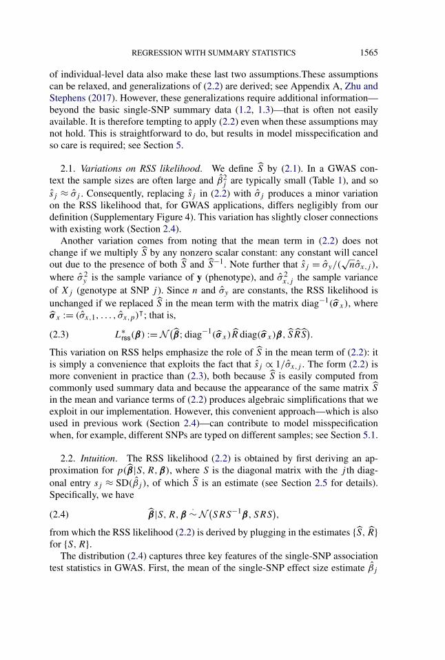
2.1. Variations on RSS likelihood. We define S by (2.1). In a GWAS con-text the sample sizes are often large and β2

j are typically small (Table 1), and sosj ≈ σj . Consequently, replacing sj in (2.2) with σj produces a minor variationon the RSS likelihood that, for GWAS applications, differs negligibly from ourdefinition (Supplementary Figure 4). This variation has slightly closer connectionswith existing work (Section 2.4).

Another variation comes from noting that the mean term in (2.2) does notchange if we multiply S by any nonzero scalar constant: any constant will cancelout due to the presence of both S and S−1. Note further that sj = σy/(

√nσx,j ),

where σ 2y is the sample variance of y (phenotype), and σ 2

x,j the sample varianceof Xj (genotype at SNP j ). Since n and σy are constants, the RSS likelihood isunchanged if we replaced S in the mean term with the matrix diag−1(σ x), whereσ x := (σx,1, . . . , σx,p)ᵀ; that is,

(2.3) L∗rss(β) := N

(β;diag−1(σ x)R diag(σ x)β, SRS

).

This variation on RSS helps emphasize the role of S in the mean term of (2.2): itis simply a convenience that exploits the fact that sj ∝ 1/σx,j . The form (2.2) ismore convenient in practice than (2.3), both because S is easily computed fromcommonly used summary data and because the appearance of the same matrix S

in the mean and variance terms of (2.2) produces algebraic simplifications that weexploit in our implementation. However, this convenient approach—which is alsoused in previous work (Section 2.4)—can contribute to model misspecificationwhen, for example, different SNPs are typed on different samples; see Section 5.1.

2.2. Intuition. The RSS likelihood (2.2) is obtained by first deriving an ap-proximation for p(β|S,R,β), where S is the diagonal matrix with the j th diag-onal entry sj ≈ SD(βj ), of which S is an estimate (see Section 2.5 for details).Specifically, we have

(2.4) β|S,R,β·∼ N

(SRS−1β, SRS

),

from which the RSS likelihood (2.2) is derived by plugging in the estimates {S, R}for {S,R}.

The distribution (2.4) captures three key features of the single-SNP associationtest statistics in GWAS. First, the mean of the single-SNP effect size estimate βj


depends on both its own effect and the effects of all SNPs that it “tags” (i.e., ishighly correlated with):

(2.5) E(βj |S,R,β) = sj ·p∑

i=1

rij s−1i βi,

where rij is the (i, j)-entry of R. Second, the likelihood incorporates the fact thatthe estimated single-SNP effects are heteroscedastic:

(2.6) Var(βj |S,R,β) = s2j ≈ s2

j = (nX

ᵀj Xj

)−1yᵀy.

Since s2j is roughly proportional to (X

ᵀj Xj )

−1, the likelihood takes account of dif-ferences in the informativeness of SNPs due to their variation in allele frequencyand imputation quality [Guan and Stephens (2008)]. Third, single-SNP test statis-tics at SNPs in LD are correlated:

(2.7) Corr(βj , βk|S,R,β) = rjk,

for any pair of SNP j and k.Note that SNPs in LD with one another have “correlated” test statistics {βj } for

two distinct reasons. First, they share a “signal,” which is captured in the mean term(2.5). This shared signal becomes a correlation if the true effects β are assumedto arise from some distribution and are then integrated out. Second, they share“noise,” which is captured in the correlation term (2.7). This latter correlation oc-curs even in the absence of signal (β = 0) and is due to the fact that the summarydata are computed on the same samples. If the summary data were computed onindependent sets of individuals, then this latter correlation would disappear (Sec-tion 5.1).

2.3. Connection with the full-data likelihood. When individual-level data areavailable the multiple regression model is

(2.8) y|X,β, τ ∼N(Xβ, τ−1I

).

If we further assume the residual variance τ−1 is known, model (2.8) specifiesa likelihood for β , which we denote Lmvn(β;y,X, τ). The following proposi-tion gives conditions under which this full-data likelihood and RSS likelihood areequivalent.

PROPOSITION 2.1. Let Rsam denote the sample LD matrix computed fromthe genotypes X of the study cohort, Rsam := D−1XᵀXD−1 where D := diag(d),d := (‖X1‖, . . . ,‖Xp‖)ᵀ, ‖Xj‖ := (X

ᵀj Xj )

1/2.

If n > p, τ−1 = n−1yᵀy and R = Rsam, then

(2.9) logLrss(β; β, S, R) − logLmvn(β;y,X, τ) = C,

where C is some constant that does not depend on β .


The assumption n > p in Proposition 2.1 could possibly be relaxed, but cer-tainly simplifies the proof. The key assumption then is τ−1 = n−1yᵀy; that is, thetotal variance in y explained by X is negligible. This will typically not hold in agenome-wide context, but might hold, approximately, when fine mapping a smallgenomic region since SNPs in a small region typically explain a very small pro-portion of phenotypic variation.2 Hence, provided that R = Rsam, RSS and its full-data counterpart will produce approximately the same inferential results in smallregions. This is illustrated through simulations in Section 4.1 (Figure 1); see alsoChen et al. (2015).

2.4. Connection with previous work. The RSS likelihood is connected to sev-eral previous approaches to inference from summary data, as we now describe.[These connections are precise for the variation on the RSS likelihood with sj = σj

(Section 2.1), which differs negligibly in practice from (2.2).]In the simplest case, if R is an identity matrix, then β|β, S ∼ N (β, S2), which

is the implied likelihood based on the standard confidence interval [Efron (1993)].Wakefield (2009) has recently popularized this likelihood for calculation of ap-proximate Bayes factors; see also Stephens (2017).

If we let z denote the vector of single-SNP z-scores, z := S−1β , and plug {S, R}into (2.4), then

(2.10) z|S, R,β ∼ N(RS−1β, R

).

This is analogous to the likelihood proposed in Hormozdiari et al. (2014), z ∼N (Rν, R), where they refer to ν as the “noncentrality parameter.” If further β = 0,then z ∼ N (0, R), a result that has been used for multiple testing adjustment [e.g.,Seaman and Müller-Myhsok (2005); Lin (2005)], gene-based association detection[e.g., Liu et al. (2010)] and z-score imputation [e.g., Lee et al. (2013)].

If β is given a prior distribution that assumes zero mean and independenceacross all j , that is, p(β|S, R) = ∏

j p(βj |S, R), E(βj |S, R) = 0, then integrat-

ing β out in (2.10) yields E(z2j |S, R) = 1 + ∑p

i=1 r2ij s

−2i E(β2

i |S, R). This is a keyelement of LD score regression [Bulik-Sullivan et al. (2015)]; see Appendix C,Zhu and Stephens (2017), for further details and discussion.

2.5. Derivation. We treat the (unobserved) genotypes of each individual, xi

(the ith row of X), as being independent and identically distributed draws fromsome population. Without loss of generality, assume these have been centered,by subtracting the mean, so that E(xi ) = 0. Let σx,j > 0 denote the populationstandard deviation (SD) of xij , and R denote the p×p positive definite population

2There are exceptions; for example, the human leukocyte antigen region is estimated to explain11–37% of the heritability of rheumatoid arthritis [Kurkó et al. (2013)].

1568X

.ZH

UA

ND

M.ST

EPH

EN

S

TABLE 1Summary of per-SNP sample squared correlation {c2

j } and sample size {nj } for 42 large GWAS performed in European-ancestry individuals. The fullnames of phenotypes and corresponding references are provided in Supplementary Table 1. The five-number summaries and histograms are across SNPs.

The sample correlation cj between phenotype and genotype of SNP j is defined as cj := (‖y‖ · ‖Xj‖)−1(Xᵀj y). Note that

c2j = (nj σ 2

j + β2j )−1β2

j = (nj s2j )−1β2

j , and cjp→ cj . The SD of sample sizes per SNP {nj } is NA when {nj } are not publicly available

GWAS phenotype # of SNPs(million)

log10(c2) log10(n)

Min Q1 Median Q3 Max Histogram Median Mean SD

Height (GIANT, 2010) 2.82 −12.64 −6.25 −5.60 −5.12 −2.90 5.26 5.26 NAHeight (GIANT, 2014) 2.53 −10.74 −6.06 −5.41 −4.93 −2.54 5.40 5.37 0.09BMI (GIANT, 2015) 2.54 −10.89 −6.30 −5.65 −5.18 −2.66 5.37 5.34 0.09WHRadjBMI (GIANT, 2015) 2.53 −10.81 −6.11 −5.46 −4.99 −2.81 5.15 5.13 0.08

HDL (GLGC, 2010) 2.68 −10.78 −5.90 −5.25 −4.77 −1.23 5.00 4.89 0.33HDL (GLGC, 2013) 2.43 −10.16 −5.89 −5.25 −4.78 −1.59 4.97 4.97 0.06LDL (GLGC, 2010) 2.68 −10.72 −5.89 −5.23 −4.75 −1.44 4.98 4.87 0.33LDL (GLGC, 2013) 2.42 −9.95 −5.89 −5.24 −4.78 −1.40 4.95 4.95 0.06TC (GLGC, 2010) 2.68 −10.33 −5.91 −5.25 −4.77 −1.38 5.00 4.89 0.33TC (GLGC, 2013) 2.43 −10.28 −5.91 −5.26 −4.79 −1.79 4.98 4.97 0.06TG (GLGC, 2010) 2.68 −10.55 −5.89 −5.24 −4.76 −1.17 4.98 4.87 0.33TG (GLGC, 2013) 2.42 −10.07 −5.88 −5.24 −4.78 −1.90 4.96 4.96 0.06Cigarettes per day (TAG, 2010) 2.46 −14.16 −5.84 −5.19 −4.73 −2.69 4.87 4.87 NASmoking age of onset (TAG, 2010) 2.43 −11.27 −5.82 −5.18 −4.73 −3.44 4.87 4.87 NA

Ever smoked (TAG, 2010) 2.45 −11.89 −5.82 −5.17 −4.71 −3.44 4.87 4.87 NAFormer smoker (TAG, 2010) 2.45 −12.68 −5.83 −5.19 −4.73 −3.40 4.87 4.87 NAYears of education (SSGAC, 2013) 2.14 −7.10 −5.70 −5.30 −4.85 −3.51 5.10 5.10 NACollege or not (SSGAC, 2013) 2.25 −8.37 −5.93 −5.33 −4.88 −3.39 5.10 5.10 NADepressive (SSGAC, 2016) 6.03 −7.44 −6.00 −5.46 −5.01 −3.60 5.21 5.21 NANeuroticism (SSGAC, 2016) 6.04 −7.88 −5.92 −5.45 −4.98 −3.29 5.23 5.23 NASchizophrenia (PGC, 2014) 9.43 −12.50 −6.01 −5.35 −4.88 −3.04 5.18 5.18 NA

RE

GR

ESSIO

NW

ITH

SUM

MA

RY

STAT

ISTIC

S1569

TABLE 1(Continued)

GWAS phenotype # of SNPs(million)

log10(c2) log10(n)

Min Q1 Median Q3 Max Histogram Median Mean SD

Alzheimer (IGAP, 2013) 7.04 −11.20 −5.69 −5.04 −4.57 −1.33 4.73 4.73 NACAD (CARDIoGRAM, 2011) 2.42 −17.43 −5.84 −5.18 −4.71 −2.74 4.91 4.88 0.08

T2D (DIAGRAM, 2012) 2.09 −7.83 −6.00 −5.49 −5.13 −2.93 4.80 4.78 0.10Hb (HaemGen, 2012) 2.58 −9.79 −5.64 −4.99 −4.52 −2.47 4.74 4.68 0.15MCHC (HaemGen, 2012) 2.57 −9.72 −5.62 −4.98 −4.51 −2.50 4.70 4.65 0.15

MCH (HaemGen, 2012) 2.58 −10.24 −5.56 −4.91 −4.44 −2.02 4.67 4.62 0.14MCV (HaemGen, 2012) 2.59 −11.02 −5.61 −4.96 −4.48 −2.09 4.71 4.66 0.15

PCV (HaemGen, 2012) 2.59 −10.67 −5.59 −4.94 −4.47 −2.70 4.69 4.63 0.14RBC (HaemGen, 2012) 2.56 −8.92 −5.55 −4.91 −4.45 −2.11 4.69 4.63 0.15FGadjBMI (MAGIC, 2012) 2.61 −11.63 −5.70 −5.07 −4.61 −2.10 4.76 4.76 NA

FIadjBMI (MAGIC, 2012) 2.60 −11.54 −5.65 −5.02 −4.56 −2.96 4.71 4.71 NAHeart rate (HRgene, 2013) 2.52 −12.08 −5.88 −5.23 −4.76 −2.88 4.95 4.93 0.07Serum urate (GUGC, 2013) 2.44 −10.36 −5.95 −5.30 −4.83 −1.49 5.04 5.03 0.02Gout (GUGC, 2013) 2.54 −12.17 −5.80 −5.15 −4.69 −2.68 4.84 4.84 0.01RA (Okada et al, 2014) 7.70 −8.16 −5.44 −4.97 −4.55 −1.09 4.77 4.77 NAIBD (IIBDGC, 2015) 12.70 −13.05 −5.49 −4.84 −4.38 −2.07 4.54 4.54 NACD (IIBDGC, 2015) 12.27 −12.97 −5.28 −4.62 −4.16 −1.89 4.32 4.32 NAUC (IIBDGC, 2015) 12.24 −12.69 −5.40 −4.75 −4.28 −2.07 4.44 4.44 NACAD (CARDIoGRAM+C4D, 2015) 9.46 −15.00 −6.26 −5.61 −5.14 −2.62 5.27 5.27 NA

MI (CARDIoGRAM+C4D, 2015) 9.29 −18.89 −6.22 −5.56 −5.09 −2.69 5.22 5.22 NAANM (ReproGen, 2015) 2.09 −7.40 −5.44 −4.84 −4.56 −2.16 4.84 4.84 NA


correlation matrix, and so Var(xi ) := �x := diag(σ x) · R · diag(σ x), where σ x :=(σx,1, . . . , σx,p)ᵀ.

We assume that the phenotypes y := (y1, . . . , yn)ᵀ are generated from the

multiple-SNP model (1.1), where E(ε) = 0 and Var(ε) = τ−1In. We also assumethat X, ε and β are mutually independent.

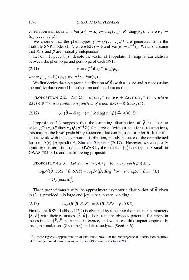
Let c := (c1, . . . , cp)ᵀ denote the vector of (population) marginal correlationsbetween the phenotype and genotype of each SNP:

(2.11) c := σ−1y diag−1(σ x)μxy

where μxy := E(xiyi) and σ 2y := Var(yi).

We first derive the asymptotic distribution of β (with n → ∞ and p fixed) usingthe multivariate central limit theorem and the delta method.

PROPOSITION 2.2. Let � := σ 2y diag−1(σ x)(R + �(c))diag−1(σ x), where

�(c) ∈Rp×p is a continuous function of c and �(c) =O(maxj c2

j ):

(2.12)√

n(β − diag−1(σ x)R diag(σ x)β

) d→ N (0,�).

Proposition 2.2 suggests that the sampling distribution of β is close toN (diag−1(σ x)R diag(σ x)β, n−1�) for large n. Without additional assumptions,this may be the best3 probability statement that can be used to infer β . It is diffi-cult to work with this asymptotic distribution, mainly because of the complicatedform of �(c) [Appendix A, Zhu and Stephens (2017)]. However, we can justifyignoring this term in a typical GWAS by the fact that {c2

j } are typically small inGWAS (Table 1), and the following proposition.

PROPOSITION 2.3. Let S := n− 12 σy diag−1(σ x). For each β ∈ R

p ,

logN(β;SRS−1β, SRS

) − logN(β;diag−1(σ x)R diag(σ x)β, n−1�

)= Op

(maxj c

2j

).

These propositions justify the approximate asymptotic distribution of β givenin (2.4), provided n is large and {c2

j } close to zero, yielding

(2.13) Lrss(β; β, S,R) := N(β;SRS−1β, SRS

).

Finally, the RSS likelihood (2.2) is obtained by replacing the nuisance parameters{S,R} with their estimates {S, R}. There remains obvious potential for errors inthe estimates {S, R} to impact inference, and we assess this impact empiricallythrough simulations (Section 4) and data analyses (Section 6).

3A more rigorous approximation of likelihood based on the convergence in distribution requiresadditional technical assumptions; see Boos (1985) and Sweeting (1986).


3. Bayesian inference based on summary data. Using the RSS likelihood,we perform Bayesian inference for the multiple regression coefficients.

3.1. Prior specification. If {S,R} were known, then one could performBayesian inference by specifying a prior on β:

(3.1) p(β|β, S,R)︸︷︷︸Posterior

∝ p(β|S,R,β)︸︷︷︸Likelihood

·p(β|S,R)︸︷︷︸Prior

.

To deal with unknown {S,R}, the RSS likelihood (2.2) approximates the likelihoodin (3.1) by replacing {S,R} with their estimates {S, R}. We take a similar approachto prior specification: we specify a prior p(β|S,R) and replace {S,R} with {S, R}.

Our prior specification is based on the prior from Zhou, Carbonetto andStephens (2013) which was designed for analysis of individual-level GWAS data.This prior assumes that β is independent of R a priori, with the prior on βj beinga mixture of two normal distributions

(3.2) βj ∼ πN(0, σ 2

B + σ 2P

) + (1 − π)N(0, σ 2

P

).

The motivation is that the first (“sparse”) component can capture rare “large” ef-fects, while the second (“polygenic”) component can capture large numbers ofvery small effects. To specify priors on the variances, {σ 2

B,σ 2P }, Zhou, Carbonetto

and Stephens (2013) introduce two free parameters h,ρ ∈ [0,1], where h4 repre-sents, roughly, the proportion of variance in y explained by X, and ρ representsthe proportion of genetic variance explained by the sparse component. They writeσ 2

B and σ 2P as functions of π,h,ρ and place independent priors on the hyperpa-

rameters (π,h,ρ):

(3.3) logπ ∼ U(log(1/p), log 1

), h ∼ U(0,1), ρ ∼ U(0,1);

see Zhou, Carbonetto and Stephens (2013) for details.Here we must modify this prior slightly because the original definitions of σB

and σP depend on the genotypes X (which here are unknown) and the residualvariance τ−1 (which does not appear in our likelihood). Specifically, we define

(3.4) σ 2B(S) := hρ

(π

p∑j=1

n−1s−2j

)−1

, σ 2P (S) := h(1 −ρ)

( p∑j=1

n−1s−2j

)−1

,

where sj is the j th diagonal entry of S. Because ns2j = σ 2

y σ−2x,j , definitions (3.4)

ensure that the effect sizes of both components do not depend on n, and havethe same measurement unit as the phenotype y. Further, with these definitions,

4Parameter h is related to heritability [Visscher, Hill and Wray (2008)], which is often denoted

as h2 in genetics literature. We use h here to keep notation consistent with previous closely relatedwork [Guan and Stephens (2011), Zhou, Carbonetto and Stephens (2013)].


ρ and h have interpretations similar to those in previous work. Specifically, ρ =(πσ 2

B)/(πσ 2B + σ 2

P ), and so it represents the expected proportion of total geneticvariation explained by the sparse components. Parameter h represents, roughly,the proportion of the total variation in y explained by X, as formalized by thefollowing proposition:

PROPOSITION 3.1. If β|S is distributed as (3.2), with (3.4), then

(3.5) E[V (Xβ)

] = h · E[V (y)

],

where V (Xβ) and V (y) are the sample variance of Xβ and y, respectively.

Because of its similarity with the prior from the “Bayesian sparse linear mixedmodel” [BSLMM, Zhou, Carbonetto and Stephens (2013)], we refer to our mod-ified prior as BSLMM. We also implement a version of this prior where ρ = 1.This sets the polygenic variance σ 2

P = 0, making the prior on β sparse, and cor-responds closely to the prior from the “Bayesian variable selection regression”[BVSR, Guan and Stephens (2011)]. We therefore refer to this special case asBVSR here.

3.2. Posterior inference and computation. We use Markov chain Monte Carlo(MCMC) to sample from the posterior distribution of β; see Appendix B, Zhu andStephens (2017), for details.

To fit the RSS-BSLMM model, we implement a new algorithm that is differentfrom previous work [Zhou, Carbonetto and Stephens (2013)]. Instead of integrat-ing out β analytically, we perform MCMC sampling on β directly. Most of theMCMC updates in this algorithm have linear complexity, with only a few “ex-pensive” exceptions. The costs of these “expensive” updates are further reducedfrom being cubic in the total number of SNPs to being quadratic by leveraging thebanded structure of the LD matrix R [Wen and Stephens (2010)].

Our algorithm of fitting the RSS-BVSR model largely follows those developedin Guan and Stephens (2011) which exploit sparsity. Specifically, computationtime per iteration scales cubically with the number of SNPs with nonzero effects,which is much smaller than the total number of SNPs under sparse assumptions.Setting a fixed maximum number of nonzero effects, and/or using the banded LDstructure to guide variable selection, can further improve computational perfor-mance, but we do not use these strategies here.

All computations were performed on a Linux system with a single Intel E5-2670 2.6 GHz or AMD Opteron 6386 SE processor. Computation times for simu-lation studies and data analyses are shown in Supplementary Figure 5 and Supple-mentary Table 6, respectively. Software implementing the methods is available athttps://github.com/stephenslab/rss.

Compared with existing summary-based methods, an important practical ad-vantage of RSS is that multiple tasks can be performed using the same posteriorsample of β . Here we focus on estimating PVE (SNP heritability) and detectingmultiple-SNP associations.

https://github.com/stephenslab/rss


3.2.1. Estimating PVE. Given the full data {X,y} and the true value of {β, τ }in model (2.8), Guan and Stephens (2011) define the PVE as

(3.6) PVE(β, τ ) := V (Xβ)/(τ−1 + V (Xβ)

).

By this definition, PVE reflects the total proportion of phenotypic variation ex-plained by available genotypes. Guan and Stephens (2011) then estimate PVE us-ing the posterior sample of {β, τ }.

Because X is unknown here, we cannot compute PVE as defined above even ifβ and τ were known. Moreover, τ does not appear in our inference procedure. Forthese reasons we introduce the “Summary PVE” (SPVE) as an analogue of PVEfor our setting:

(3.7) SPVE(β) := ∑i,j

rij βiβj√(nσ 2

i + β2i )(nσ 2

j + β2j )

.

This definition is motivated by noting that PVE can be approximated by replacingτ−1 with V(y) − V (Xβ):

(3.8) PVE ≈ V (Xβ)

V (y)= ∑

i,j

Xᵀi Xj

yᵀyβiβj = ∑

i,j

rsamij βiβj√

(nσ 2i + β2

i )(nσ 2j + β2

j ),

where rsamij is the (i, j)-entry of the (unknown) sample LD matrix of the study

cohort (Rsam), which we approximate in SPVE by rij , and the last equation in (3.8)holds because of (1.2)–(1.3). Simulations using both synthetic and real genotypesshow that SPVE is a highly accurate approximation to PVE, given the true valueof β (Supplementary Figure 1).

We infer PVE using the posterior draws of SPVE, which are obtained by com-puting SPVE(β(i)) for each sampled value β(i) from our MCMC algorithms. Un-like the original PVE (3.6), the definition of SPVE (3.7) is not bounded above by 1.Although we have not seen any estimates above 1 in our simulations or data anal-yses, we expect this could occur if the posterior of β is poorly simulated and/or R

is severely misspecified.

3.2.2. Detecting genome-wide associations. Under the BVSR prior, a naturalsummary of the evidence for a SNP being associated with phenotype is the pos-terior inclusion probability (PIP), Pr(βj �= 0|y,X). Similarly, we define the PIPbased on summary data

(3.9) SPIP(j) := Pr(βj �= 0|β, S, R).

Here we estimate SPIP(j) by the proportion of MCMC draws for which βj �= 0.[We also provide a Rao–Blackwellized estimate [Casella and Robert (1996), Guanand Stephens (2011)] in Appendix B, Zhu and Stephens (2017).]


4. Simulations. We benchmark the RSS method through simulations usingreal genotypes from the Wellcome Trust Case Control Consortium (2007) (specif-ically, the 1458 individuals from the UK Blood Service Control Group) and sim-ulated phenotypes. To reduce computation, the simulations use genotypes from asingle chromosome (12,758 SNPs on chromosome 16). One consequence of thisis that the simulated effect sizes per SNP in some scenarios are often larger thanwould be expected in a typical GWAS (Table 1 and Supplementary Figure 3). Thisis, in some ways, not an ideal case for RSS because the likelihood derivation as-sumes that effect sizes are small (Proposition 2.3). We use the simulations to (i) in-vestigate the effect of different choices for R, and (ii) demonstrate that inferencesfrom RSS agree well with both the simulation ground truth, and with results frommethods based on the full data (specifically, BVSR and BSLMM implemented inthe software package GEMMA [Zhou and Stephens (2012)]).

4.1. Choice of LD matrix. The LD matrix R plays a key role in the RSS like-lihood, as well as in previous work using summary data [e.g., Bulik-Sullivan et al.(2015), Hormozdiari et al. (2014), Yang et al. (2012)]. One simple choice for R,commonly used in previous work, is the sample LD matrix computed from a suit-able “reference panel” that is deemed similar to the study population. This is aviable choice if the number of SNPs p is smaller than the number of individualsm in the reference panel, as the sample LD matrix is then invertible. However,for large-scale genomic applications p � m, and the sample LD matrix is not in-vertible. Our proposed solution is to use the shrinkage estimator from Wen andStephens (2010), which shrinks the off-diagonal entries of the sample LD matrixtoward zero, resulting in an invertible matrix.

The shrinkage-based estimate of R can result in improved inference even ifp < m. To illustrate this, we performed a small simulation study, with 982 SNPswithin the ±5 Mb region surrounding the gene IL27. We simulated 20 independentdatasets, each with 10 causal SNPs and PVE = 0.2. (We also performed simula-tions with the true PVE being 0.02 and 0.002; see Supplementary Figure 2.) Foreach dataset, we ran RSS-BVSR with two strategies for computing R from a ref-erence panel (here, the 1480 control individuals in the WTCCC 1958 British BirthCohort): the sample LD matrix (RSS-P), and the shrinkage-based estimate (RSS).We compared results with analyses using the full data (GEMMA-BVSR), and alsowith our RSS approach using the cohort LD matrix (RSS-C), which by Proposi-tion 2.1 should produce results similar to the full data analysis. The results (Fig-ure 1) show that using the shrinkage-based estimate for R produces consistentlymore accurate inferences—both for estimating PVE and detecting associations—than using the reference sample LD matrix, and indeed provides similar accuracyto the full data analysis.

4.2. Estimating PVE from summary data. Here we use simulations to assessthe performance of RSS for estimating PVE. Using the WTCCC genotypes from


FIG. 1. Comparison of PVE estimation and association detection on three types of LD matrix:cohort sample LD (RSS-C), shrinkage panel sample LD (RSS) and panel sample LD (RSS-P). Per-formance of estimating PVE is measured by the root of the mean square error (RMSE), where a lowervalue indicates better performance. Performance of detecting associations is measured by the areaunder the curve (AUC), where a higher value indicates better performance.

12,758 SNPs on chromosome 16, we simulated phenotypes under two genetic ar-chitectures:

• Scenario 1.1 (sparse): randomly select 50 “causal” SNPs, with effects comingfrom N (0,1); effects of remaining SNPs are zero.

• Scenario 1.2 (polygenic): randomly select 50 “causal” SNPs, with effects com-ing from N (0,1); effects of remaining SNPs come from N (0,0.0012).

For each scenario we simulated datasets with true PVE ranging from 0.05 to 0.5(in steps of 0.05, with 50 independent replicates for each PVE). We ran RSS-BVSR on Scenario 1.1, and RSS-BSLMM on Scenario 1.2. Figure 2 summarizesthe resulting PVE estimates. The estimated PVEs generally correspond well withthe true values, but with a noticeable upward bias when the true PVE is large. Wespeculate that this upward bias is due to deviations from the assumption of smalleffects underlying RSS in Proposition 2.3. (Note that with 50 causal SNPs andPVE = 0.5, on average each causal SNP explains 1% of the phenotypic variance,which is substantially higher than in typical GWAS; thus the upward bias in atypical GWAS may be less than in these simulations.)

Next, we compare accuracy of PVE estimation using summary versus full data.With the genotype data as above, we consider two scenarios:

• Scenario 2.1 (sparse): simulate a fixed number T of causal SNPs (T =10,100,1000), with effect sizes coming from N (0,1), and the effect sizes ofthe remaining SNPs are zero;


FIG. 2. Comparison of true PVE with estimated PVE (posterior median) in Scenarios 1.1 (sparse)and 1.2 (polygenic). The dotted lines indicate the true PVEs, and the bias of estimates is reported onthe top of each box plot. Each box plot summarizes results from 50 replicates.

• Scenario 2.2 (polygenic): simulate two groups of causal SNPs, the first groupcontaining a small number T of large-effect SNPs (T = 10,100,1000), plusanother larger group of 10,000 small-effect SNPs; the large effects are drawnfrom N (0,1), the small effects are drawn from N (0,0.0012), and the effects ofthe remaining SNPs are zero.

For each scenario we created datasets with true PVE 0.2 and 0.6 (20 indepen-dent replicates for each parameter combination). For Scenario 2.1 we comparedresults from the summary data methods (RSS-BVSR and RSS-BSLMM) withthe corresponding full data methods (GEMMA-BVSR and GEMMA-BSLMM).For Scenario 2.2 we compared only the BSLMM methods since the BVSR-basedmethods, which assume effects are sparse, are not well suited to this setting interms of both computation and accuracy [Zhou, Carbonetto and Stephens (2013)];see also Appendix B, Zhu and Stephens (2017). Figure 3 summarizes the re-sults. With modest true PVE (0.2), GEMMA-BVSR and RSS-BVSR perform bet-ter than other methods when the true model is very sparse (e.g., Scenario 2.1,T = 10), whereas GEMMA-BSLMM and RSS-BSLMM perform better when thetrue model is highly polygenic (e.g., Scenario 2.2, T = 1000). When the true PVEis large (0.6), the summary-based methods show an upward bias [Figures 3(b)and 3(d)], consistent with Figure 2. This bias is less severe when the true signalsare more “diluted” (e.g., T = 1000), consistent with our speculation above that thebias is due to deviations from the “small effects” assumption. Overall, as expected,the summary data methods perform slightly less accurately than the full data meth-ods. However, using different modeling assumptions (BVSR versus BSLMM) hasa bigger impact on the results than using summary versus full data.


FIG. 3. Comparison of PVE estimates (posterior median) from GEMMA and RSS in Scenarios 2.1and 2.2. The accuracy of estimation is measured by the relative RMSE, which is defined as the RMSEbetween the ratio of the estimated over true PVEs and 1. Relative RMSE for each method is reported(percentages on top of box plots). The true PVEs are shown as the solid horizontal lines. Each boxplot summarizes results from 20 replicates.

4.3. Power to detect associations from summary data. Previous studies usingindividual-level data have shown that the multiple-SNP model can have higherpower to detect genetic associations than single-SNP analyses [e.g., Guan andStephens (2011), Hoggart et al. (2008), Moser et al. (2015), Servin and Stephens(2007)]. Here we compare the power of multiple-SNP analyses based on summary


data with those based on individual-level data. Specifically, we focus on compar-ing RSS-BVSR with GEMMA-BVSR because the BVSR-based methods naturallyselect the associated SNPs (whereas BSLMM assumes that all SNPs are associ-ated).

To compare associations detected by RSS-BVSR and GEMMA-BVSR, we sim-ulated data under Scenario 2.1 above. With BVSR analyses, associations are mostrobustly assessed at the level of regions rather than at the level of individual SNPs[Guan and Stephens (2011)], and so we compare the association signals from thetwo methods in sliding 200-kb windows (sliding each window 100 kb at a time).Specifically, for each 200-kb region, and each method, we sum the PIPs of SNPsin the region to obtain the “Expected Number of included SNPs” (ENS), whichsummarizes the strength of association in that region. Results (Figure 4) show astrong correlation between the ENS values from the summary and individual dataacross different numbers of causal variants and PVE values. Consequently, thesummary data analyses have similar power to detect associations as the full dataanalyses (Figure 5). As above, the agreement of RSS-BVSR with GEMMA-BVSRis highest when PVE is diluted among many SNPs (e.g., T = 1000).

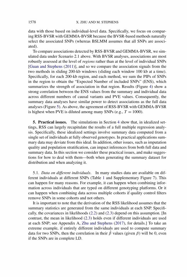
5. Practical issues. The simulations in Section 4 show that, in idealized set-tings, RSS can largely recapitulate the results of a full multiple regression analy-sis. Specifically, these idealized settings involve summary data computed from asingle set of individuals at fully observed genotypes. In practical applications sum-mary data may deviate from this ideal. In addition, other issues, such as imputationquality and population stratification, can impact inferences from both full data andsummary data. In this section we consider these practical issues, and make sugges-tions for how to deal with them—both when generating the summary dataset fordistribution and when analyzing it.

5.1. Data on different individuals. In many studies data are available on dif-ferent individuals at different SNPs (Table 1 and Supplementary Figure 7). Thiscan happen for many reasons. For example, it can happen when combining infor-mation across individuals that are typed on different genotyping platforms. Or itcan happen when combining data across multiple cohorts if quality control filtersremove SNPs in some cohorts and not others.

It is important to note that the derivation of the RSS likelihood assumes that thesummary statistics are generated from the same individuals at each SNP. Specifi-cally, the covariances in likelihoods (2.2) and (2.3) depend on this assumption. [Incontrast, the mean in likelihood (2.3) holds even if different individuals are usedat each SNP; see Appendix A, Zhu and Stephens (2017), for details.] To take anextreme example, if entirely different individuals are used to compute summarydata for two SNPs, then the correlation in their β values (given β) will be 0, evenif the SNPs are in complete LD.


FIG. 4. Comparison of the 200-kb region posterior expected numbers of included SNPs (ENS) forGEMMA-BVSR (x-axis) and RSS-BVSR (y-axis) based on the simulation study of Scenario 2.1. Eachpoint is a 200-kb genomic region, colored according to whether it contains at least one causal SNP(reddish purple “*”) or not (bluish green “+”).


FIG. 5. Trade-off between true and false positives for GEMMA-BVSR (dash) and RSS-BVSR (solid)in simulations of Scenario 2.1.


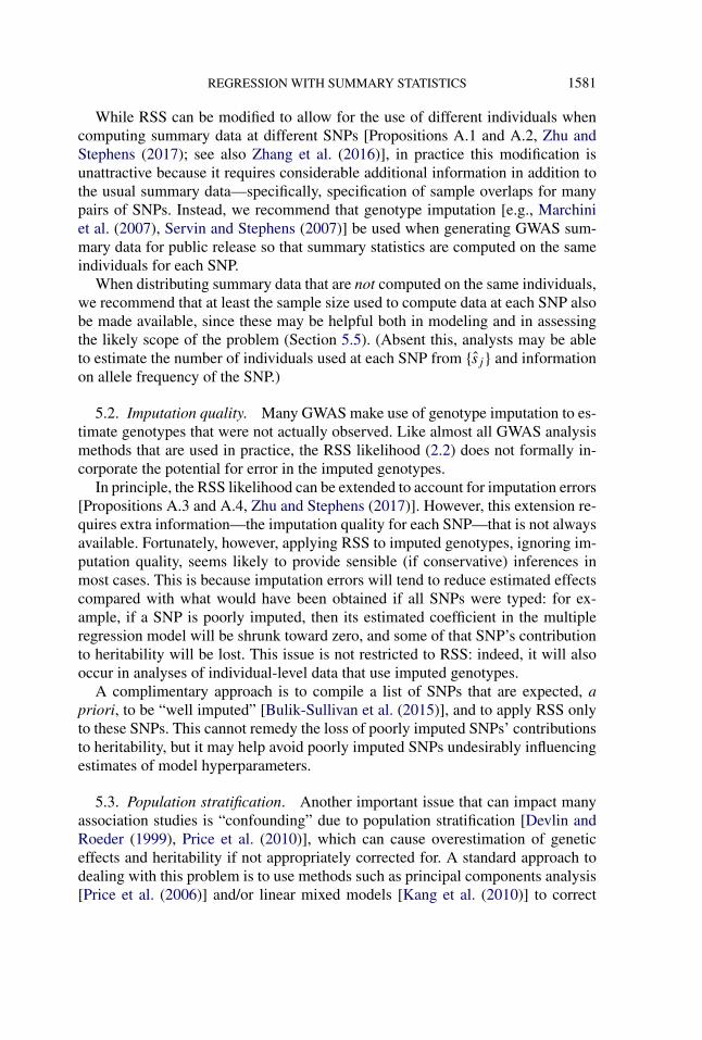
While RSS can be modified to allow for the use of different individuals whencomputing summary data at different SNPs [Propositions A.1 and A.2, Zhu andStephens (2017); see also Zhang et al. (2016)], in practice this modification isunattractive because it requires considerable additional information in addition tothe usual summary data—specifically, specification of sample overlaps for manypairs of SNPs. Instead, we recommend that genotype imputation [e.g., Marchiniet al. (2007), Servin and Stephens (2007)] be used when generating GWAS sum-mary data for public release so that summary statistics are computed on the sameindividuals for each SNP.

When distributing summary data that are not computed on the same individuals,we recommend that at least the sample size used to compute data at each SNP alsobe made available, since these may be helpful both in modeling and in assessingthe likely scope of the problem (Section 5.5). (Absent this, analysts may be ableto estimate the number of individuals used at each SNP from {sj } and informationon allele frequency of the SNP.)

5.2. Imputation quality. Many GWAS make use of genotype imputation to es-timate genotypes that were not actually observed. Like almost all GWAS analysismethods that are used in practice, the RSS likelihood (2.2) does not formally in-corporate the potential for error in the imputed genotypes.

In principle, the RSS likelihood can be extended to account for imputation errors[Propositions A.3 and A.4, Zhu and Stephens (2017)]. However, this extension re-quires extra information—the imputation quality for each SNP—that is not alwaysavailable. Fortunately, however, applying RSS to imputed genotypes, ignoring im-putation quality, seems likely to provide sensible (if conservative) inferences inmost cases. This is because imputation errors will tend to reduce estimated effectscompared with what would have been obtained if all SNPs were typed: for ex-ample, if a SNP is poorly imputed, then its estimated coefficient in the multipleregression model will be shrunk toward zero, and some of that SNP’s contributionto heritability will be lost. This issue is not restricted to RSS: indeed, it will alsooccur in analyses of individual-level data that use imputed genotypes.

A complimentary approach is to compile a list of SNPs that are expected, apriori, to be “well imputed” [Bulik-Sullivan et al. (2015)], and to apply RSS onlyto these SNPs. This cannot remedy the loss of poorly imputed SNPs’ contributionsto heritability, but it may help avoid poorly imputed SNPs undesirably influencingestimates of model hyperparameters.

5.3. Population stratification. Another important issue that can impact manyassociation studies is “confounding” due to population stratification [Devlin andRoeder (1999), Price et al. (2010)], which can cause overestimation of geneticeffects and heritability if not appropriately corrected for. A standard approach todealing with this problem is to use methods such as principal components analysis[Price et al. (2006)] and/or linear mixed models [Kang et al. (2010)] to correct


for stratification. These methods require access to the individual-level genotypedata, and so cannot be used directly by analysts with access only to summary data.Instead they must be used by analysts who are computing the summary data forpublic distribution: doing so should substantially reduce the effects of confoundingon summary data analyses, including RSS.

A complementary approach to dealing with population stratification is to di-rectly model its effects on the summary data. One recent and innovative approachto this is LD score regression [Bulik-Sullivan et al. (2015)], which uses the inter-cept of a regression of association signal versus “LD score” to assess the effectsof confounding. Along similar lines, we could modify the RSS likelihood to in-corporate the effects of confounding by introducing an additional dispersion pa-rameter (7.1); see Appendix C, Zhu and Stephens (2017). This modification wouldnot require extra information, and may have an additional benefit of improvingrobustness of RSS to other model misspecification issues (e.g., genotyping error,mismatches between LD in the reference panel and sample). However, this modi-fication requires additional computation [some linear algebra simplifications usedin (2.2) do not hold for (7.1)], and we have not yet implemented it.

5.4. Filtering and diagnostics. Some of the recommendations above can onlybe implemented when the summary data are being computed from individual datafor public distribution, and not at a later stage when only the summary data areavailable. This raises the question, what can analysts with only access to summarydata do to check that their results are likely reliable? This may be the trickiestpart of summary data analysis: even with access to the full individual-level data,it can be hard to assess all sources of bias and error. Recognizing that there isno universal approach that will guarantee reliable results, we nonetheless hope toprovide some useful suggestions.

Since the RSS likelihood (2.2) defines a statistical model, it is possible to per-form a model fit diagnostic check. A generic approach to model checking (e.g.,common in linear regression) is to first fit the model, compute residuals that mea-sure deviations of observations from expected values, and then discard outlyingobservations before refitting the model. We have implemented an approach alongthese lines for identifying outlying SNPs as follows. First, after fitting the model,we compute the residual (the difference between the observed β and its fittedexpected value) at each SNP. We then perform a “leave-one-out” (LOO) checkon each residual: we compute its conditional expectation and variance given theresiduals at all other SNPs, and compute a diagnostic z-score based on how theobserved residual compares with this expectation and variance; see Appendix D,Zhu and Stephens (2017), for details. This approach targets SNPs whose summarydata are most inconsistent with data at other nearby SNPs in LD. If the modelis correctly specified for a given SNP, then its diagnostic z-score approximatelyfollows a standard normal distribution, from which a large deviation indicates po-tential misspecification. To assess robustness of RSS fit, one can filter out SNPswith large diagnostic z-scores, and refit the RSS model on the remaining SNPs.


Other simpler filters are of course possible, and multiple filters can be usedtogether. One widely used filter simply discards SNPs with sample sizes lowerthan a certain cutoff [Pickrell (2014)]. This can reduce problems caused by SNPsbeing typed on different subsets of individuals discussed above (Section 5.1). An-other possibility is to filter out SNPs that are in very strong LD with one another,since these have the potential for producing severe misspecification (Section 5.5).Some advantages of the model-based LOO diagnostic include that it could de-tect model misspecification problems from several sources—including genotypingerror or misspecification of the LD matrix R—and not only those caused by typ-ing of different individuals at different SNPs. Also, the sample size filter cannotbe used unless the sample size for each SNP is made available, which is not al-ways the case (Table 1). Finally, choice of threshold for the diagnostic z-scorecan be guided by the standard normal distribution; in contrast, selecting principledthresholds for sample sizes seems less straightforward (and a stringent thresholdcan yield conservative results; see Supplementary Figure 8). On the other hand, theLOO diagnostic may tend to filter out SNPs that show a particularly strong signal(if they are not in LD with other SNPs), an undesirable property that should beremembered when interpreting results post-filtering (Supplementary Figure 9).

5.5. Extreme example. One way to help avoid problems with model misspec-ification is to be aware of the most severe ways in which things can go wrong.In this vein, we offer one illustrative example that we encountered when applyingRSS to the summary data of a blood lipid GWAS [Global Lipids Genetics Consor-tium (2013)].

Table 2 shows summary statistics for high-density lipoprotein (HDL) choles-terol for seven SNPs in the gene ADH5 that are in complete LD with one anotherin the reference panel (1000 Genomes European r2 = 1). If summary data were

TABLE 2Example of problems that can arise due to severe model misspecification. The table reports the

sample sizes (nj ), single-SNP effect size estimates (βj ), SEs (σj ), and 1-SNP BFs of seven SNPsthat are in complete LD in the reference panel (1000 Genomes, European ancestry). The 2-SNP BFsreported are for rs7683704 with each of the other SNPs. These unreasonably large 2-SNP BFs are

due to model misspecification

SNP nj βj σj 1-SNP log10 BF 2-SNP log10 BF r2

rs7683704 187,124 0.0096 0.0058 −0.676 NA 1.0rs13125919 94,311 0.0038 0.0079 −1.084 172.638 1.0rs4699701 94,311 0.0054 0.0081 −1.028 88.364 1.0rs17595424 94,274 0.0055 0.0081 −1.024 83.925 1.0rs11547772 94,311 0.0056 0.0081 −1.021 79.756 1.0rs7683802 94,311 0.0056 0.0081 −1.021 79.756 1.0rs4699699 94,311 0.0058 0.0081 −1.013 71.580 1.0


computed on the same set of individuals at each SNP, then they would be expectedto vary very little among SNPs that are in such strong LD. And, indeed, the RSSlikelihood captures this expectation. However, in this case we see that the sum-mary data actually vary considerably at some SNPs. The differences between oneSNP (rs7683704) and the others are likely explained by the fact that this SNP wastyped on more individuals: data at this SNP come from both GWAS (up to 94,595individuals) and Metabochip arrays (up to 93,982 individuals). Thus this is an ex-ample of model misspecification due to SNPs being typed on different individuals.However, another SNP, rs13125919, also shows notable differences in summarydata from the other SNPs for reasons that are unclear to us. (This highlights a chal-lenge of working with summary data—it is difficult to investigate the source ofsuch anomalies without access to individual data.)

Whatever the reasons, applying RSS to these data results in severe model mis-specification: based on their LD patterns, RSS expects data at these SNPs to bealmost identical, but they are not. This severe model misspecification can lead tounreliable results. For example, we used the RSS likelihood (2.2) to compute the1-SNP and 2-SNP Bayes factors (BFs) [as in Servin and Stephens (2007); see alsoChen et al. (2015)]. None of the SNPs shows evidence for marginal associationwith HDL (log10 1-SNP BF are all negative, indicating evidence for the null).However, the 2-SNP BFs for rs7683704 together with any of the other SNPs areunreasonably large due to the severe model misspecification.

We emphasize that this is an extreme example, chosen to highlight the worstthings that can go wrong. We did not come across any examples like this in spot-checks of results from the adult human height data below (Section 6). For sim-ulations illustrating the effects of less extreme model misspecification on PVEestimation see Supplementary Figure 6.

6. Analysis of summary data on adult height. We applied RSS to summarystatistics from a GWAS of human adult height involving 253,288 individuals ofEuropean ancestry typed at ∼1.06 million SNPs [Wood et al. (2014)]. Access-ing the individual-level data would be a considerable undertaking; in contrast, thesummary data are easily and freely available.5

Following the protocol from Bulik-Sullivan et al. (2015), we filtered out poorlyimputed SNPs and then removed SNPs absent from the genetic map of HapMapEuropean-ancestry population Release 24 [Frazer et al. (2007)]. To avoid negativerecombination rate estimates, we excluded SNPs in regions where the genome as-sembly had been rearranged. We also removed triallelic sites by manual inspectionin BioMart [Smedley et al. (2015)]. This left 1,064,575 SNPs retained for analy-sis. We estimated the LD matrix R using phased haplotypes from 379 European-ancestry individuals in the 1000 Genomes Project Consortium (2010).

5https://www.broadinstitute.org/collaboration/giant/index.php/GIANT_consortium_data_files

https://www.broadinstitute.org/collaboration/giant/index.php/GIANT_consortium_data_files


Although the summary data were generated after genotype imputation to thesame reference panel [Section 1.1.2, Supplementary Note of Wood et al. (2014)],only 65% of the 1,064,575 analyzed SNPs were computed from the total sample(Supplementary Figure 7). This is because SNP filters applied by the consortiumseparately in each cohort often filtered out SNPs from a subset of cohorts [Sec-tion 1.1.4, Supplementary Note of Wood et al. (2014)]. As shown in Appendix Aof Zhu and Stephens (2017), properly accounting for the sample difference wouldrequire sample overlap information that is not publicly available. Instead, we di-rectly applied the original RSS likelihood (2.2) to the summary data. As discussedin Section 5.1, this simplification results in model misspecification. To assess theimpact of this, in addition to the primary analysis using all the summary data,we also performed secondary analyses after applying the LOO residual diagnosticdescribed in Section 5.4 to filter out SNPs whose diagnostic z-scores exceeded athreshold (2 or 3).

To reduce computation time and hardware requirement, we separately analyzedeach of the 22 autosomal chromosomes so that all chromosomes were run in par-allel in a computer cluster. In our analysis, each chromosome used a single CPUcore. To assess convergence of the MCMC algorithm, we ran the algorithm oneach dataset multiple times; results agreed well among runs (results not shown),suggesting no substantial problems with convergence. Here we report results froma single run on each chromosome with 2 million iterations. The CPU time of RSS-BVSR ranged from 1 to 36 hours, and the time of RSS-BSLMM ranged from 4 to36 hours (Supplementary Table 6).

We first inferred PVE (SNP heritability) from these summary data. Figure 6shows the estimated total and per-chromosome PVEs based on RSS-BVSR andRSS-BSLMM. For both methods, we can see an approximately linear relation-ship between PVE and chromosome length, consistent with a genetic architecturewhere many causal SNPs each contribute a small amount to PVE (a.k.a. “poly-genicity”), and consistent with previous results using a mixed linear model [Yanget al. (2011)] on three smaller individual-level datasets (number of SNPs: 593,521–687,398; sample size: 6293–15,792). By summing PVE estimates across all 22chromosomes, we estimated the total autosomal PVE to be 52.4%, with 95% cred-ible interval [50.4%, 54.5%] using RSS-BVSR, and 52.1%, with 95% credibleinterval [50.3%, 53.9%] using RSS-BSLMM. Our estimates are consistent with,but more precise than, previous estimates based on individual-level data from sub-sets of this GWAS. Specifically, Wood et al. (2014) estimated PVE as 49.8%, withstandard error 4.4%, from individual-level data of five cohorts (number of SNPs:0.97–1.12 million; sample size: 1145–5668). The increased precision of the PVEestimates illustrates one benefit of being able to analyze summary data with a largesample size.

One caveat to these results is that the RSS likelihood (2.2) ignores confoundingsuch as population stratification (Section 5.3). Here the summary data were gen-erated using genomic control, principal components and linear mixed effects to


FIG. 6. Posterior inference of PVE (SNP heritability) for adult human height. Panel A: posteriordistributions of the total PVE, where the interval spanned by the arrows is the 95% confidence inter-val from Wood et al. (2014). Panel B: posterior median and 95% credible interval for PVE of eachchromosome against the chromosome length, where each dot is labeled with chromosome numberand the lines are fitted by simple linear regression (solid: RSS-BVSR; dash: RSS-BSLMM). The sim-ple linear regression output is shown in Supplementary Table 2. The data to reproduce Panel B areprovided in Supplementary Table 3.

control for population stratification within each cohort [Section 1.1.3, Supplemen-tary Note of Wood et al. (2014)]. Thus we might hope that confounding has limitedimpact on PVE estimation. However, it is difficult to be sure that all confoundinghas been completely removed, and any remaining confounding could upwardlybias our estimated PVE. (Unremoved confounding could similarly bias estimatesbased on individual-level data.)

Next, we used RSS-BVSR to detect multiple-SNP associations, and comparedresults with previous analyses of these summary data. Using a stepwise selectionstrategy proposed by Yang et al. (2012), Wood et al. (2014) reported a total of 697genome-wide significant SNPs (GWAS hits). Among them, 531 SNPs were withinthe ±40-kb regions with estimated ENS ≥ 1. Since only 384 GWAS hits wereincluded in our filtered set of SNPs, we expected a higher replication rate for theseincluded GWAS hits. Taking a region of ±40-kb around each of these 384 SNPs,our analysis identified almost all of these regions (371/384) as showing a strongsignal for association (estimated ENS ≥ 1). Only 125 of the 384 SNPs showed,individually, strong evidence for inclusion (estimated SPIP > 0.9). This suggeststhat, perhaps unsurprisingly, many of the reported associations are likely driven bya SNP in LD with the one identified in the original analysis.

To assess the potential for RSS to identify novel putative loci associated with hu-man height, we estimated the ENS for ±40-kb windows across the whole genome.We identified 5194 regions with ENS ≥ 1, of which 2138 are putatively novel in


that they are not near any of the previous 697 GWAS hits (distance > 1 Mb). Someof these 2138 regions are overlapping, but this nonetheless represents a large num-ber of potential novel associations for further investigation. We manually examinedthe putatively novel regions with highest ENS, and identified several loci harbor-ing genes that seem plausibly related to height. These include the gene SCUBE1,which is critical in promoting bone morphogenetic protein signaling [Liao, Tsaoand Yang (2016)], the gene WWOX, which is linked to skeletal system morpho-genesis [Aqeilan et al. (2008), Del Mare et al. (2011)], the gene IRX5, which isessential for proximal and anterior skeletal formation [Li et al. (2014)], and thegene ALX1 (a.k.a. CART1), which is involved in bone development [Iioka et al.(2003)]; see Supplementary Table 5 for the full list of putatively new loci (ENS> 3).

Finally, to check for misspecification, we performed the LOO residual-baseddiagnostic. Specifically, we ran the LOO residual imputation using the RSS-BVSR output, and then refitted the models on the filtered SNPs (absolute LOOz-score ≤ 2). This resulted in a substantial reduction in PVE estimates (RSS-BVSR: 34.0%, [32.9%, 35.0%]; RSS-BSLMM: 45.3%, [44.7%, 46.0%]). How-ever, this may reflect the fact that the filter removed 12% of SNPs, possibly biasedtoward SNPs showing the association signal (Supplementary Figure 9). By com-parison, association results were more robust. Among the ±40-kb regions aroundthe previous GWAS hits, our reanalysis identified 532 of the 697 total hits, and373 of the 384 included hits. Moving the ±40-kb window across the genome, weidentified 6426 regions with ENS ≥ 1, of which 2798 were at least 1 Mb awayfrom the 697 GWAS hits. Results are similar based on a less stringent threshold(3) (Supplementary Table 4).

7. Discussion. We have presented a novel Bayesian method to infer multiplelinear regression coefficients using simple linear regression summary statistics,and demonstrated its application in GWAS. On both simulated and real data ourmethod produces results comparable to methods based on individual-level data.Compared with existing summary-based methods, our approach takes advantageof an explicit likelihood for the multiple regression coefficients, and thus provides aunified framework for various genome-wide analyses. We theoretically extend thisframework to capture certain features of GWAS summary data, and provide practi-cal suggestions when the theoretical extensions cannot be easily implemented. Weillustrate the applications of our framework on heritability estimation and associ-ation detection. Other potential applications include training phenotype predictionmodels, prioritizing causal variants and testing gene-level effects.

We view the present work as the first stage of what could be done with RSSusing GWAS summary statistics. One possibility for future work is to modify theRSS likelihood (2.2) to incorporate confounding by introducing an additional dis-persion parameter a:

(7.1) β|S,R,β ∼N(SRS−1β, SRS + na · S2)

.


From model (7.1) we can derive relationships to LD score regression [Bulik-Sullivan et al. (2015)], which distinguishes confounding biases from polygenic-ity using GWAS summary statistics; see Appendix C, Zhu and Stephens (2017),for details. Another important extension is to integrate additional genomic infor-mation into the prior distributions. For instance, Carbonetto and Stephens (2013)allow the prior probability of each SNP being included to depend on a covariate,such as biological pathway membership,

(7.2) βj |S ∼ (1 − πj )δ0 + πjN(0, σ 2(S)

), logit(πj ) = θ0 + θaj ,

where aj = 1 when SNP j is in the pathway. Unlike prior (3.2), prior (7.2) re-flects that biologically related gene sets might preferentially harbor associatedSNPs, essentially integrating the idea of gene set enrichment into GWAS [Wang,Li and Hakonarson (2010)]. As a second example, some functional categories ofthe genome could contribute disproportionately to the heritability of complex traits[Gusev et al. (2014)], which could be incorporated by letting the prior variance ofthe SNP effects depend on functional categorization, for example, by

(7.3) βj |S ∼ N(0, σ 2

j (S)), log

(σ 2

j

) = w0 +G∑

g=1

wgfj,g,

where fj,g = 1 when SNP j belongs to category g, w0 captures the baseline (log)heritability and {wg} reflect the contribution of each category. This could providea different way to partition heritability by functional annotation using GWAS sum-mary statistics [Finucane et al. (2015)].

Acknowledgments. We thank the Editor, Associate Editor and two anony-mous referees for their constructive comments. We thank Xin He, Rina FoygelBarber, Peter Carbonetto, Yongtao Guan, Xiaoquan Wen and Xiang Zhou for help-ful discussions. We thank Raman Shah and John Zekos for technical support. Thisstudy makes use of data generated by the Wellcome Trust Case Control Consor-tium. A full list of the investigators who contributed to the generation of the datais available from www.wtccc.org.uk. Data on adult human height have been con-tributed by investigators of the Genetic Investigation of Anthropometric Traits (GI-ANT) consortium. This work was completed in part with resources provided by theUniversity of Chicago Research Computing Center.

SUPPLEMENTARY MATERIAL

Supplement to “Bayesian large-scale multiple regression with summarystatistics from genome-wide association studies” (DOI: 10.1214/17-AOAS1046SUPP; .pdf). This file contains all the Appendices, Supplementary Ta-bles and Figures referenced in the main text.

http://www.wtccc.org.uk

http://dx.doi.org/10.1214/17-AOAS1046SUPP



REFERENCES

1000 GENOMES PROJECT CONSORTIUM (2010). A map of human genome variation frompopulation-scale sequencing. Nature 467 1061–1073.

AQEILAN, R. I., HASSAN, M. Q., DE BRUIN, A., HAGAN, J. P., VOLINIA, S., PALUMBO, T.,HUSSAIN, S., LEE, S.-H., GAUR, T., STEIN, G. S. et al. (2008). The WWOX tumor suppressoris essential for postnatal survival and normal bone metabolism. J. Biol. Chem. 283 21629–21639.

BOOS, D. D. (1985). A converse to Scheffé’s theorem. Ann. Statist. 13 423–427. MR0773179BULIK-SULLIVAN, B., LOH, P.-R., FINUCANE, H., RIPKE, S., YANG, J., PSYCHIATRIC GE-

NOMICS CONSORTIUM SCHIZOPHRENIA WORKING GROUP, PATTERSON, N., DALY, M. J.,PRICE, A. L. and NEALE, B. M. (2015). LD score regression distinguishes confounding frompolygenicity in genome-wide association studies. Nat. Genet. 47 291–295.

CARBONETTO, P. and STEPHENS, M. (2013). Integrated enrichment analysis of variants and path-ways in genome-wide association studies indicates central role for IL-2 signaling genes in type 1diabetes, and cytokine signaling genes in crohn’s disease. PLoS Genet. 9 e1003770.

CASELLA, G. and ROBERT, C. P. (1996). Rao–Blackwellisation of sampling schemes. Biometrika83 81–94. MR1399157

CHEN, W., LARRABEE, B. R., OVSYANNIKOVA, I. G., KENNEDY, R. B., HARALAMBIEVA, I. H.,POLAND, G. A. and SCHAID, D. J. (2015). Fine mapping causal variants with an approximateBayesian method using marginal test statistics. Genetics 200 719–736.

DEL MARE, S., KUREK, K. C., STEIN, G. S., LIAN, J. B. and AQEILAN, R. I. (2011). Role of theWWOX tumor suppressor gene in bone homeostasis and the pathogenesis of osteosarcoma. Am.J. Cancer Res. 1 585.

DEVLIN, B. and ROEDER, K. (1999). Genomic control for association studies. Biometrics 55 997–1004.

DONNELLY, P. (2008). Progress and challenges in genome-wide association studies in humans. Na-ture 456 728–731.

EFRON, B. (1993). Bayes and likelihood calculations from confidence intervals. Biometrika 80 3–26.MR1225211

EHRET, G. B., LAMPARTER, D., HOGGART, C. J., WHITTAKER, J. C., BECKMANN, J. S., KUTA-LIK, Z., GENETIC INVESTIGATION OF ANTHROPOMETRIC TRAITS CONSORTIUM et al. (2012).A multi-SNP locus-association method reveals a substantial fraction of the missing heritability.Am. J. Hum. Genet. 91 863–871.

EVANGELOU, E. and IOANNIDIS, J. P. (2013). Meta-analysis methods for genome-wide associationstudies and beyond. Nat. Rev. Genet. 14 379–389.

FINUCANE, H. K., BULIK-SULLIVAN, B., GUSEV, A., TRYNKA, G., RESHEF, Y., LOH, P.-R.,ANTTILA, V., XU, H., ZANG, C., FARH, K. et al. (2015). Partitioning heritability by functionalannotation using genome-wide association summary statistics. Nat. Genet. 47 1228–1235.

FRAZER, K. A., BALLINGER, D. G., COX, D. R., HINDS, D. A., STUVE, L. L., GIBBS, R. A.,BELMONT, J. W., BOUDREAU, A., HARDENBOL, P., LEAL, S. M. et al. (2007). A secondgeneration human haplotype map of over 3.1 million SNPs. Nature 449 851–861.

GLOBAL LIPIDS GENETICS CONSORTIUM (2013). Discovery and refinement of loci associated withlipids levels. Nat. Genet. 45 1274–1283.

GUAN, Y. and STEPHENS, M. (2008). Practical issues in imputation-based association mapping.PLoS Genet. 4 e1000279.

GUAN, Y. and STEPHENS, M. (2011). Bayesian variable selection regression for Genome-wide as-sociation studies and other large-scale problems. Ann. Appl. Stat. 5 1780–1815. MR2884922

GUAN, Y. and WANG, K. (2013). Whole-genome multi-SNP-phenotype association analysis. In Ad-vances in Statistical Bioinformatics 224–243. Cambridge Univ. Press, Cambridge. MR3155921

http://www.ams.org/mathscinet-getitem?mr=0773179






GUSEV, A., LEE, S. H., TRYNKA, G., FINUCANE, H., VILHJÁLMSSON, B. J., XU, H., ZANG, C.,RIPKE, S., BULIK-SULLIVAN, B., STAHL, E., KÄHLER, A. K., HULTMAN, C. M., PUR-CELL, S. M., MCCARROLL, S. A., DALY, M., PASANIUC, B., SULLIVAN, P. F., NEALE, B. M.,WRAY, N. R., RAYCHAUDHURI, S. and PRICE, A. L. (2014). Partitioning heritability of regula-tory and cell-type-specific variants across 11 common diseases. Am. J. Hum. Genet. 95 535–552.

HOGGART, C. J., WHITTAKER, J. C., IORIO, M. D. and BALDING, D. J. (2008). Simultane-ous analysis of all SNPs in genome-wide and re-sequencing association studies. PLoS Genet.4 e1000130.

HORMOZDIARI, F., KOSTEM, E., KANG, E. Y., PASANIUC, B. and ESKIN, E. (2014). Identifyingcausal variants at loci with multiple signals of association. Genetics 198 497–508.

IIOKA, T., FURUKAWA, K., YAMAGUCHI, A., SHINDO, H., YAMASHITA, S. and TSUKAZAKI, T.(2003). P300/CBP acts as a coactivator to cartilage homeoprotein-1 (Cart1), paired-like homeo-protein, through acetylation of the conserved lysine residue adjacent to the homeodomain. J. BoneMiner. Res. 18 1419–1429.

KANG, H. M., SUL, J. H., SERVICE, S. K., ZAITLEN, N. A., KONG, S.-Y., FREIMER, N. B.,SABATTI, C., ESKIN, E. et al. (2010). Variance component model to account for sample structurein genome-wide association studies. Nat. Genet. 42 348–354.

KURKÓ, J., BESENYEI, T., LAKI, J., GLANT, T. T., MIKECZ, K. and SZEKANECZ, Z. (2013).Genetics of rheumatoid arthritis—A comprehensive review. Clin. Rev. Allergy Immunol. 45 170–179.

LEE, D., BIGDELI, T. B., RILEY, B. P., FANOUS, A. H. and BACANU, S.-A. (2013). DIST: Directimputation of summary statistics for unmeasured SNPs. Bioinformatics 29 2925–2927.

LEE, D., WILLIAMSON, V. S., BIGDELI, T. B., RILEY, B. P., FANOUS, A. H., VLADIMIROV, V. I.and BACANU, S.-A. (2015). JEPEG: A summary statistics based tool for gene-level joint testingof functional variants. Bioinformatics 31 1176–1182.

LI, D., SAKUMA, R., VAKILI, N. A., MO, R., PUVIINDRAN, V., DEIMLING, S., ZHANG, X.,HOPYAN, S. and HUI, C.-C. (2014). Formation of proximal and anterior limb skeleton requiresearly function of Irx3 and Irx5 and is negatively regulated by Shh signaling. Dev. Cell 29 233–240.

LIAO, W.-J., TSAO, K.-C. and YANG, R.-B. (2016). Electrostatics and N-glycan-mediated mem-brane tethering of SCUBE1 is critical for promoting bone morphogenetic protein signalling.Biochem. J. 473 661–672.

LIN, D. (2005). An efficient Monte Carlo approach to assessing statistical significance in genomicstudies. Bioinformatics 21 781–787.

LIU, J. Z., MCRAE, A. F., NYHOLT, D. R., MEDLAND, S. E., WRAY, N. R., BROWN, K. M.,HAYWARD, N. K., MONTGOMERY, G. W., VISSCHER, P. M., MARTIN, N. G. et al. (2010).A versatile gene-based test for genome-wide association studies. Am. J. Hum. Genet. 87 139–145.

LOH, P.-R., TUCKER, G., BULIK-SULLIVAN, B. K., VILHJALMSSON, B. J., FINUCANE, H. K.,CHASMAN, D. I., RIDKER, P. M., NEALE, B. M., BERGER, B., PATTERSON, N. et al. (2015).Efficient Bayesian mixed model analysis increases association power in large cohorts. Nat. Genet.47 284–290.

MARCHINI, J., HOWIE, B., MYERS, S., MCVEAN, G. and DONNELLY, P. (2007). A new multipointmethod for genome-wide association studies by imputation of genotypes. Nat. Genet. 39 906–913.

MCCARTHY, M. I., ABECASIS, G. R., CARDON, L. R., GOLDSTEIN, D. B., LITTLE, J., IOANNI-DIS, J. P. and HIRSCHHORN, J. N. (2008). Genome-wide association studies for complex traits:Consensus, uncertainty and challenges. Nat. Rev. Genet. 9 356–369.

MOSER, G., LEE, S. H., HAYES, B. J., GODDARD, M. E., WRAY, N. R. and VISSCHER, P. M.(2015). Simultaneous discovery, estimation and prediction analysis of complex traits using aBayesian mixture model. PLoS Genet. 11 e1004969.


NATURE GENETICS (2012). Asking for more. Nat. Genet. 44 733.NEWCOMBE, J., CONTI, V. and RICHARDSON, S. (2016). JAM: a scalable bayesian framework for

joint analysis of marginal SNP effects. Genet. Epidemiol. 40 188–201.PALLA, L. and DUDBRIDGE, F. (2015). A fast method that uses polygenic scores to estimate the

variance explained by genome-wide marker panels and the proportion of variants affecting a trait.Am. J. Hum. Genet. 97 250–259.

PARK, J.-H., WACHOLDER, S., GAIL, M. H., PETERS, U., JACOBS, K. B., CHANOCK, S. J. andCHATTERJEE, N. (2010). Estimation of effect size distribution from genome-wide associationstudies and implications for future discoveries. Nat. Genet. 42 570–575.

PEISE, E., FABREGAT-TRAVER, D. and BIENTINESI, P. (2015). High performance solutions forbig-data GWAS. Parallel Comput. 42 75–87.

PICKRELL, J. K. (2014). Joint analysis of functional genomic data and genome-wide associationstudies of 18 human traits. Am. J. Hum. Genet. 94 559–573.

PRICE, A. L., PATTERSON, N. J., PLENGE, R. M., WEINBLATT, M. E., SHADICK, N. A. andREICH, D. (2006). Principal components analysis corrects for stratification in genome-wide as-sociation studies. Nat. Genet. 38 904–909.

PRICE, A. L., ZAITLEN, N. A., REICH, D. and PATTERSON, N. (2010). New approaches to popu-lation stratification in genome-wide association studies. Nat. Rev. Genet. 11 459–463.

PRITCHARD, J. K. and PRZEWORSKI, M. (2001). Linkage disequilibrium in humans: Models anddata. Am. J. Hum. Genet. 69 1–14.

SABATTI, C. (2013). Multivariate linear models for GWAS. In Advances in Statistical Bioinformat-ics (K.-A. Do, Z. S. Qin and M. Vannucci, eds.) 188–207. Cambridge Univ. Press, Cambridge.MR3155918

SEAMAN, S. R. and MÜLLER-MYHSOK, B. (2005). Rapid simulation of P values for product meth-ods and multiple-testing adjustment in association studies. Am. J. Hum. Genet. 76 399–408.

SERVIN, B. and STEPHENS, M. (2007). Imputation-based analysis of association studies: Candidateregions and quantitative traits. PLoS Genet. 3 e114.

SMEDLEY, D., HAIDER, S., DURINCK, S., PANDINI, L., PROVERO, P., ALLEN, J., ARNAIZ, O.,AWEDH, M. H., BALDOCK, R., BARBIERA, G. et al. (2015). The BioMart community portal: Aninnovative alternative to large, centralized data repositories. Nucleic Acids Res. 43 W589–W598.

STEPHENS, M. (2013). A unified framework for association analysis with multiple related pheno-types. PLoS ONE 8 e65245.

STEPHENS, M. (2017). False discovery rates: A new deal. Biostatistics 18 275–294.SWEETING, T. J. (1986). On a converse to Scheffé’s theorem. Ann. Statist. 14 1252–1256.

MR0856821VILHJALMSSON, B., YANG, J., FINUCANE, H. K., GUSEV, A., LINDSTROM, S., RIPKE, S., GEN-

OVESE, G., LOH, P.-R., BHATIA, G., DO, R. et al. (2015). Modeling linkage disequilibriumincreases accuracy of polygenic risk scores. Am. J. Hum. Genet. 97 576–592.

VISSCHER, P. M., HILL, W. G. and WRAY, N. R. (2008). Heritability in the genomics era—Concepts and misconceptions. Nat. Rev. Genet. 9 255–266.

WAKEFIELD, J. (2009). Bayes factors for genome-wide association studies: Comparison with P-values. Genet. Epidemiol. 33 79–86.

WANG, K., LI, M. and HAKONARSON, H. (2010). Analysing biological pathways in genome-wideassociation studies. Nat. Rev. Genet. 11 843–854.

WELLCOME TRUST CASE CONTROL CONSORTIUM (2007). Genome-wide association study of14,000 cases of seven common diseases and 3000 shared controls. Nature 447 661–678.

WEN, X. and STEPHENS, M. (2010). Using linear predictors to impute allele frequencies fromsummary or pooled genotype data. Ann. Appl. Stat. 4 1158–1182. MR2751337

WEN, X. and STEPHENS, M. (2014). Bayesian methods for genetic association analysis with het-erogeneous subgroups: From meta-analyses to gene-environment interactions. Ann. Appl. Stat. 8176–203. MR3191987






WOOD, A. R., ESKO, T., YANG, J., VEDANTAM, S., PERS, T. H., GUSTAFSSON, S., CHU, A. Y.,ESTRADA, K., LUAN, J., KUTALIK, Z. et al. (2014). Defining the role of common variation inthe genomic and biological architecture of adult human height. Nat. Genet. 46 1173–1186.

YANG, J., BENYAMIN, B., MCEVOY, B. P., GORDON, S., HENDERS, A. K., NYHOLT, D. R.,MADDEN, P. A., HEATH, A. C., MARTIN, N. G., MONTGOMERY, G. W. et al. (2010). CommonSNPs explain a large proportion of the heritability for human height. Nat. Genet. 42 565–569.

YANG, J., MANOLIO, T. A., PASQUALE, L. R., BOERWINKLE, E., CAPORASO, N., CUNNING-HAM, J. M., DE ANDRADE, M., FEENSTRA, B., FEINGOLD, E., HAYES, M. G. et al. (2011).Genome partitioning of genetic variation for complex traits using common SNPs. Nat. Genet. 43519–525.

YANG, J., FERREIRA, T., MORRIS, A. P., MEDLAND, S. E., MADDEN, P. A., HEATH, A. C.,MARTIN, N. G., MONTGOMERY, G. W., WEEDON, M. N., LOOS, R. J. et al. (2012). Condi-tional and joint multiple-SNP analysis of GWAS summary statistics identifies additional variantsinfluencing complex traits. Nat. Genet. 44 369–375.

ZHANG, H., WHEELER, W., HYLAND, P. L., YANG, Y., SHI, J., CHATTERJEE, N. and YU, K.(2016). A powerful procedure for pathway-based meta-analysis using summary statistics iden-tifies 43 pathways associated with type II diabetes in European populations. PLoS Genet. 12e1006122.

ZHOU, X., CARBONETTO, P. and STEPHENS, M. (2013). Polygenic modeling with Bayesian sparselinear mixed models. PLoS Genet. 9 e1003264.

ZHOU, X. and STEPHENS, M. (2012). Genome-wide efficient mixed-model analysis for associationstudies. Nat. Genet. 44 821–824.

ZHU, X. and STEPHENS, M. (2017). Supplement to “Bayesian large-scale multiple regression withsummary statistics from genome-wide association studies”. DOI:10.1214/17-AOAS1046SUPP.

DEPARTMENT OF STATISTICS

UNIVERSITY OF CHICAGO

5747 S. ELLIS AVENUE

CHICAGO, ILLINOIS 60637USAE-MAIL: [email protected]

DEPARTMENT OF STATISTICS


5747 S. ELLIS AVENUE

CHICAGO, ILLINOIS 60637USAAND

DEPARTMENT OF HUMAN GENETICS


920 E. 58TH STREET

CHICAGO, ILLINOIS 60637USAE-MAIL: [email protected]


mailto:[email protected]

mailto:[email protected]

bayesian large-scale multiple regression with summary...

Documents