bayesian indoor positioning systems presented by: eiman elnahrawy joint work with: david madigan,...
TRANSCRIPT

Bayesian Indoor Bayesian Indoor Positioning SystemsPositioning Systems
Presented by: Eiman ElnahrawyPresented by: Eiman Elnahrawy
Joint work with: David Madigan, Richard P. Martin, Joint work with: David Madigan, Richard P. Martin, Wen-Hua Ju, P. Krishnan, A.S. KrishnakumarWen-Hua Ju, P. Krishnan, A.S. Krishnakumar
Rutgers University and Avaya LabsRutgers University and Avaya Labs
Infocom 2005Infocom 2005
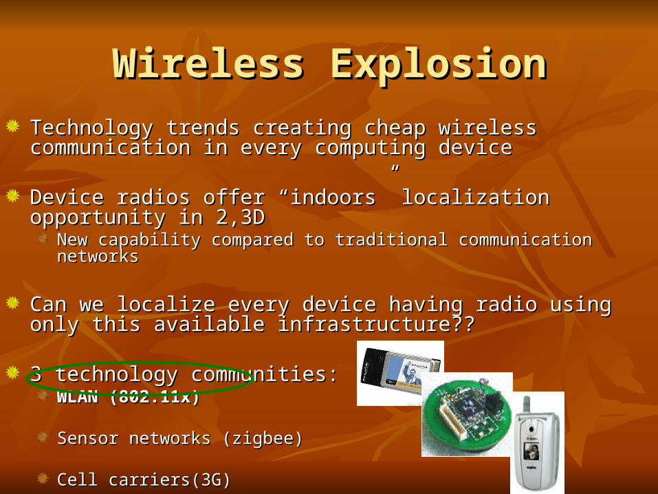
Wireless ExplosionWireless Explosion
Technology trends creating cheap wireless Technology trends creating cheap wireless communication in every computing devicecommunication in every computing device
Device radios offer “indoors” localization opportunity in Device radios offer “indoors” localization opportunity in 2,3D 2,3D
New capability compared to traditional communication New capability compared to traditional communication networks networks
Can we localize every device having radio using only Can we localize every device having radio using only this available infrastructure??this available infrastructure??
3 technology communities: 3 technology communities: WLAN (802.11x)WLAN (802.11x)
Sensor networks (zigbee)Sensor networks (zigbee)
Cell carriers(3G)Cell carriers(3G)

Radio-based LocalizationRadio-based Localization
Signal decays linearly with Signal decays linearly with log distance in laboratory log distance in laboratory setting setting
SSjj = b = b0j0j + b + b1j1j log D log Djj
DDjj = sqrt((x-x = sqrt((x-xjj))22 + (y-y + (y-yjj))22))
Use triangulation to compute Use triangulation to compute (x,y)(x,y) » Problem solved » Problem solved
Not in real life!! Not in real life!! noise, multi-path, reflections, noise, multi-path, reflections, systematic errors, etc.systematic errors, etc.
[-80,-67,-50]
Fingerprint or RSS
(x?,y?)
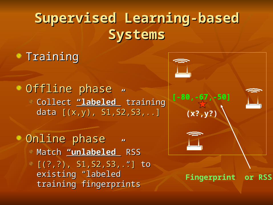
Supervised Learning-based Supervised Learning-based SystemsSystems
TrainingTraining
Offline phaseOffline phaseCollect Collect “labeled”“labeled” training training data data [(x,y), S1,S2,S3,..] [(x,y), S1,S2,S3,..]
Online phaseOnline phase Match Match “unlabeled”“unlabeled” RSS RSS
[(?,?), S1,S2,S3,..][(?,?), S1,S2,S3,..] to to existing “labeled” training existing “labeled” training fingerprintsfingerprints
[-80,-67,-50]
Fingerprint or RSS
(x?,y?)

Previous WorkPrevious Work
People have tried almost all existing supervised People have tried almost all existing supervised learning approacheslearning approaches
Well known Radar (NN)Well known Radar (NN)Probabilistic, e.g., Bayes a posteriori likelihoodProbabilistic, e.g., Bayes a posteriori likelihoodSupport Vector MachinesSupport Vector MachinesMulti-layer PerceptronsMulti-layer Perceptrons… …
[Bahl00, Battiti02, Roos02,Youssef03, Krishnan04,…][Bahl00, Battiti02, Roos02,Youssef03, Krishnan04,…]
All have a major drawback All have a major drawback Labeled training fingerprints “profiling”Labeled training fingerprints “profiling”Labor intensive (286 in 32 hrs!!)Labor intensive (286 in 32 hrs!!)May need to be repeated over the timeMay need to be repeated over the time

ContributionContribution
Why don’t we try Why don’t we try Bayesian Graphical Models Bayesian Graphical Models (BGM)(BGM)? any performance gains? ? any performance gains?
Performance-wise: comparablePerformance-wise: comparable
Minimum labeled fingerprintsMinimum labeled fingerprints
AdaptiveAdaptive
Simultaneously locate a set of objectsSimultaneously locate a set of objects
In fact it can be a zero-profiling approachIn fact it can be a zero-profiling approachNo more “labeled” training data neededNo more “labeled” training data needed
Unlabeled data can be obtained using existing data Unlabeled data can be obtained using existing data traffictraffic

LLoooocclleeTMTM
General purpose localizationGeneral purpose localization analogous to general purpose analogous to general purpose communication!communication!
Can we make finding objects in the Can we make finding objects in the physical space as easy as physical space as easy as GGoooogglle e ? ?

Can this dream come Can this dream come true?true?
We believe we are so closeWe believe we are so close
Only existing infrastructureOnly existing infrastructureLocalize with only the radios on existing Localize with only the radios on existing devicesdevices
Additional resources as performance Additional resources as performance enhancementsenhancements
Ad-hoc Ad-hoc No more labeled data No more labeled data (our contribution)(our contribution)

OutlineOutline
Motivations and GoalsMotivations and Goals
Experimental setupExperimental setup
Bayesian backgroundBayesian background
Models of increasing complexities [labeled-Models of increasing complexities [labeled-unlabeled]unlabeled]
Comparison to previous workComparison to previous work
Conclusion and Future WorkConclusion and Future Work
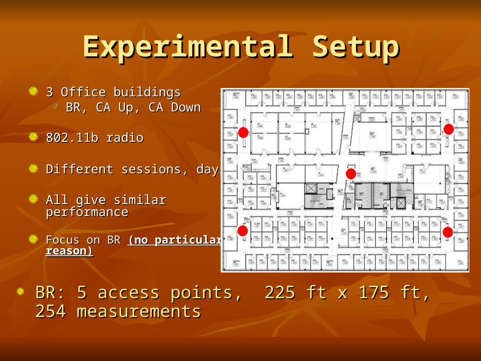
Experimental SetupExperimental Setup3 Office buildings3 Office buildings
BR, CA Up, CA DownBR, CA Up, CA Down
802.11b radio802.11b radio
Different sessions, daysDifferent sessions, days
All give similar performanceAll give similar performance
Focus on BR Focus on BR (no particular (no particular reason)reason)
BR: 5 access points, 225 ft x 175 ft, 254 BR: 5 access points, 225 ft x 175 ft, 254 measurementsmeasurements

Bayesian Graphical Bayesian Graphical ModelsModels
Encode dependencies/conditional Encode dependencies/conditional independence between variablesindependence between variables
X Y
D
S
Vertices = random variablesVertices = random variablesEdges = relationshipsEdges = relationships
Example [(X,Y), S], AP at (Example [(X,Y), S], AP at (xxb, b, yybb))Log-based signal strength propagationLog-based signal strength propagation
S = bS = b00 + b + b11 log D log D
D= sqrt((X-xD= sqrt((X-xbb))22 + (Y-y + (Y-ybb))22))

Model 1 (Simple): labeled Model 1 (Simple): labeled datadata
Xi Yi
D1
S1
b11b01 b15
D2 D3 D4 D5
S2 S3 S4 S5
b12 b13 b14b02 b03 b04 b05
Position Variables
Distances
Observed Signal Strengths
Base Station Parameters“Unknowns"
Xi ~ uniform(0, Length) Yi ~ uniform(0, Width)Si ~ N(b0i+b1ilog(Di),δi), i=1,2,3,4,5b0i ~ N(0,1000), i=1,2,3,4,5 b1i ~ N(0,1000), i=1,2,3,4,5

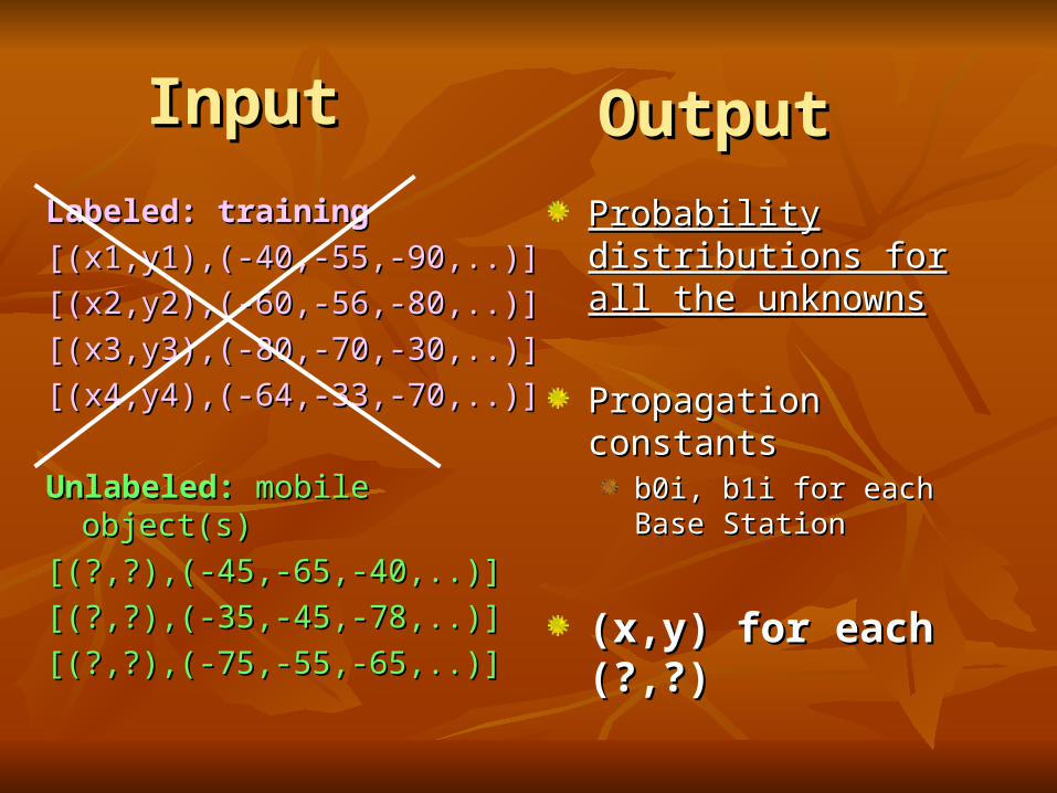
InputInput
Labeled: trainingLabeled: training
[(x1,y1),(-40,-55,-90,..)][(x1,y1),(-40,-55,-90,..)]
[(x2,y2),(-60,-56,-80,..)][(x2,y2),(-60,-56,-80,..)]
[(x3,y3),(-80,-70,-30,..)][(x3,y3),(-80,-70,-30,..)]
[(x4,y4),(-64,-33,-70,..)][(x4,y4),(-64,-33,-70,..)]
Unlabeled: Unlabeled: mobile object(s)mobile object(s)
[(?,?),(-45,-65,-40,..)][(?,?),(-45,-65,-40,..)]
[(?,?),(-35,-45,-78,..)][(?,?),(-35,-45,-78,..)]
[(?,?),(-75,-55,-65,..)][(?,?),(-75,-55,-65,..)]
Probability Probability distributions for all the distributions for all the unknown variablesunknown variables
Propagation constantsPropagation constantsb0i, b1i for each Base b0i, b1i for each Base StationStation
(x,y) for each (?,?)(x,y) for each (?,?)
OutputOutput

Great! but now how do we Great! but now how do we find the location of the find the location of the
mobile?mobile?
Closed form solution doesn’t usually exist Closed form solution doesn’t usually exist » simulation/analytic approx » simulation/analytic approx
We used We used MCMC simulationMCMC simulation (Markov (Markov Chain Monte Carlo) to generate predictive Chain Monte Carlo) to generate predictive samples from the joint distribution for samples from the joint distribution for every unknown (x,y) locationevery unknown (x,y) location

Example OutputExample Output
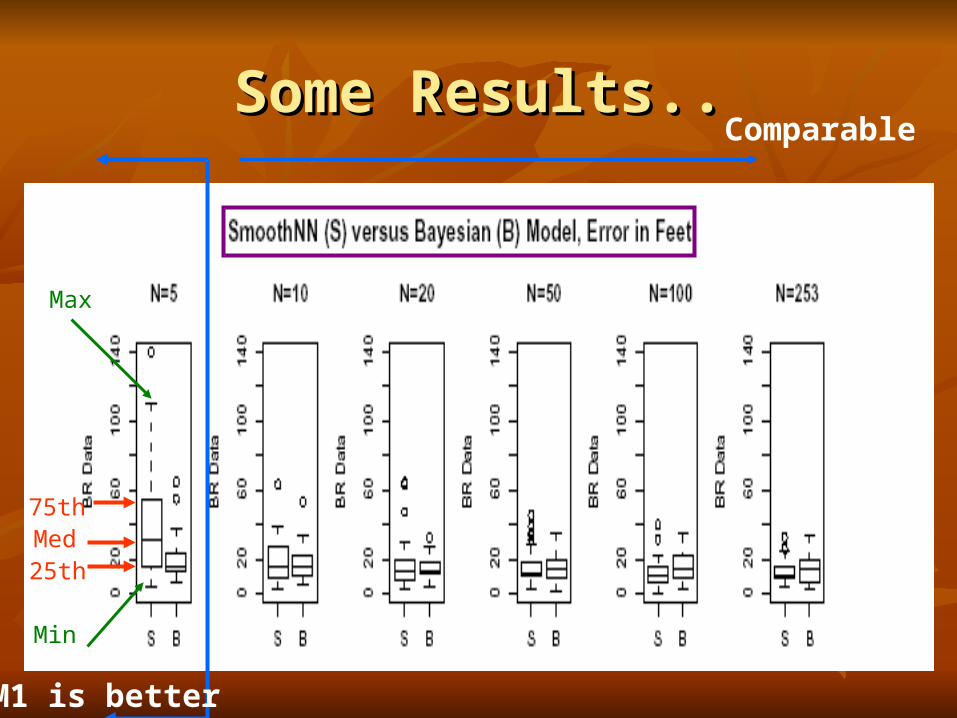
Some Results..Some Results..
M1 is better
Comparable
25thMed
75th
Min
Max

Model 2 (Hierarchical): Model 2 (Hierarchical): labeled datalabeled data
MotivationMotivation borrowing strength might provide some predictive borrowing strength might provide some predictive benefitsbenefits
Xi Yi
D1 D2 D3 D4 D5
S1 S2 S3 S4 S5
b11 b12 b13 b14 b15b01 b02 b03 b04 b05
Xi ~ uniform(0,Length)
Yi ~ uniform(0,Width)Si ~ N(b0i+b1ilog(Di), δi) b0i ~ N(b0, δb0)b1i ~ N(b1, δb1) b0 ~ N(0,1000)b1 ~ N(0,1000) δ0 ~ Gamma(0.001,0.001)δ1 ~ Gamma(0.001,0.001) i=1,2,3,4,5
Allowing any values for b’s too unconstrained!Allowing any values for b’s too unconstrained!
Assume all base-stations parametersAssume all base-stations parametersnormally distributed around a hiddennormally distributed around a hiddenvariable with a mean and variancevariable with a mean and variance

M2 behaves similar to M1, but provides improvement for very small training setsM2 behaves similar to M1, but provides improvement for very small training setsHmm, still comparable to SmoothNNHmm, still comparable to SmoothNN
More Results..More Results..Leave-one-out error (feet)
Size of labeled data
Av
era
ge
Err
or
(fe
et)
Labeled M1
Labeled Hier M2
SmoothNN
1015
2025
3035
40
0 50 100 150 200 250

Can we get reasonable estimates Can we get reasonable estimates of position of position without any labeled without any labeled
datadata??Yes! Yes!
Observe signal strengths from existing Observe signal strengths from existing data packets (unlabeled by default) data packets (unlabeled by default)
No more running around collecting No more running around collecting data.. data..
Over and over.. and over..Over and over.. and over..
InputInput
Labeled: trainingLabeled: training
[(x1,y1),(-40,-55,-90,..)][(x1,y1),(-40,-55,-90,..)]
[(x2,y2),(-60,-56,-80,..)][(x2,y2),(-60,-56,-80,..)]
[(x3,y3),(-80,-70,-30,..)][(x3,y3),(-80,-70,-30,..)]
[(x4,y4),(-64,-33,-70,..)][(x4,y4),(-64,-33,-70,..)]
Unlabeled: Unlabeled: mobile object(s)mobile object(s)
[(?,?),(-45,-65,-40,..)][(?,?),(-45,-65,-40,..)]
[(?,?),(-35,-45,-78,..)][(?,?),(-35,-45,-78,..)]
[(?,?),(-75,-55,-65,..)][(?,?),(-75,-55,-65,..)]
Probability Probability distributions for all the distributions for all the unknownsunknowns
Propagation constantsPropagation constantsb0i, b1i for each Base b0i, b1i for each Base StationStation
(x,y) for each (?,?)(x,y) for each (?,?)
OutputOutput

Model 3 (Zero Profiling)Model 3 (Zero Profiling)
Same graph as M2 Same graph as M2 (Hierarchical) but with (Hierarchical) but with (unlabeled data)(unlabeled data)
Xi Yi
D1 D2 D3 D4 D5
S1 S2 S3 S4 S5
b11 b12 b13 b14 b15b01 b02 b03 b04 b05
Hmm, why would this work?Hmm, why would this work?[1] Prior knowledge about distance-signal strength
[2] Prior knowledge that access points behave similarly

Results Close to SmoothNN, Results Close to SmoothNN, BUT…!!BUT…!!
0 50 100 150 200 250
20
40
60
80
0 50 100 150 200 250
20
40
60
80
0 50 100 150 200 250
2040
6080
Leave-one-out error (feet)
Size of input data
Av
era
ge
Err
or
in F
eet
Zero Profiling M3
SmoothNN
LABELED
UNLABELED

Other ideasOther ideas
Corridor EffectsCorridor EffectsWhat? RSS is stronger What? RSS is stronger along corridorsalong corridors
Variable c =1 if the Variable c =1 if the point shares x or y with point shares x or y with the APthe AP
No improvementsNo improvements
Informative Prior Informative Prior distributionsdistributions
S1 S2 S3 S4 S5
1 2 3 4 5
D1 D2 D3 D4 D5
YiXi
C1 C2 C3 C4 C5

Comparison to previous Comparison to previous workwork
0 10 20 30 40 50 60 70 80 90 1000
0.1
0.2
0.3
0.4
0.5
0.6
0.7
0.8
0.9
1
Distance in feet
Pro
bab
ility
Error CDF Across Algorithms
RADARProbabilisticM1-labeled
M3-unlabeledM2-labeled
•More ad-hoc
•Adaptive
•No labor investment
Conclusion and Future Conclusion and Future WorkWork
First time to actually use BGM First time to actually use BGM Considerable promise for localizationConsiderable promise for localizationPerformance comparable to existing approachesPerformance comparable to existing approachesZero profiling! (can we localize anything with a Zero profiling! (can we localize anything with a radio??)radio??)
Where are we going?Where are we going?Other modelsOther modelsVariational approximationsVariational approximationsTracking applicationsTracking applicationsMinimum extra infrastructure (more information - Minimum extra infrastructure (more information - better accuracy)!better accuracy)!

Thanks! Thanks! ☺☺