barycentric subspace analysis on the sphere and image ... filealma mater studiorum ⋅università di...
TRANSCRIPT
Alma Mater Studiorum ⋅ Università di Bologna
Scuola di Scienze
Corso di Laurea Magistrale in Matematica
Barycentric Subspace Analysis on theSphere and Image Manifolds
Relatore:Chiar.ma Prof.Giovanna Citti
Correlatore:Chiar.mo Prof.Xavier Pennec
Presentata da:Soa Farina
Sessione UnicaAnno Accademico 2016-2017

Introduction
The purpose of this thesis is to present a generalization of Principal Com-ponent Analysis (PCA) to Riemannian manifolds called Barycentric Sub-space Analysis and show some applications.
In the Euclidean case the PCA is a statistical tool of multivariate analysisthat has the purpose of reducing the dimension of the space in the presenceof a large number of data, in fact it corresponds to search the subspace whichmaximizes the variance of the data. The limit of this method arises whenwe want to work on dierentiable manifolds such as the Space of Images.For this reason, a generalization of the PCA becomes an interesting objectof study. A denition that generalizes the concept of ane subspace tomanifolds, i.e. the barycentric subspaces, was rst introduced by X. Pennecin [7]. They lead to a hierarchy of properly embedded linear subspaces ofincreasing dimension, i.e. a ag of subspaces, which generalize the notion ofane Euclidean subspaces. In the Euclidean PCA the sum of the unexplainedvariance by all the subspaces of the ag is minimized, and a similar criterionapplied to barycentric subspaces is at the basis of the Barycentric SubspaceAnalysis (BSA).
In this thesis we will present a detailed study of the method on the spheresince it can be considered as the nite dimensional projection of a set ofprobability densities that have many practical applications. This is the mostoriginal part of this thesis work. We also show an application of the barycen-tric subspace method for the study of cardiac motion in the problem of imageregistration, following the work of M.M. Rohé [13].
The thesis is organized as follows:
Chapter 1 recalls the main concepts of Dierential Geometry, such as Rie-mannian manifolds, Levi Civita connections, and geodesics. In this regard,we show that if the metric is compatible with the connection, the geodesicminimizing the functional lengths are solutions of a dierential equation thatinvolves the connection. We will therefore show that the geodesics in thesphere are the great circle. In addition, we introduce the main notions ofGroups and Lie algebras which we will use in Chapter 5 for the registration
i
ii
of images.To work with data on a manifold, we need to dene the statistical tools on
it. For this reason, in Chapter 2 the denitions of statistics on Riemannianmanifolds are presented. In fact, the measure induced by the Riemannianmetric on the manifold allows to dene probability density functions. Wefocus on the denition of expected value of a random variable and we willalso dene the mean of Fréchet and Karcher dened as the locus of the pointsthat locally or globally minimize the variance.
In Chapter 3 the denition of Barycentric Subspaces is given [7]. De-pending on the denition of mean that we choose on the manifold: Fréchet,Karcher or exponential barycenter, we obtain three types of barycentric sub-spaces: Fréchet (FBS), Karcher (KBS) or exponential (EBS). It is shownthat these three subspaces are related to each other since they are nested.In particular, the closure of the largest of these, EBS, leads to the denitionof ane subspaces on the manifold. If the manifold is complete, the anesubspaces are also complete. Finally we use the barycentric subspaces for thegeneralization of the PCA to the Riemannian manifolds, since we dene anincreasing family of barycentric subspaces that generate a ag of subspaces.The chapter ends by showing three dierent numerical methods of analysiswith barycentric subspaces.
In Chapter 4 we present an application of Barycentric Subspaces on thesphere, since the sphere can represent the space of probability density func-tions which can be used to model the frequency of pixel values in images. Werst clarify that the space of probability density functions can be identiedwith a sphere in L2, and we will restrict to a nite dimensional space in viewof the implementation. Then we study the Riemannian geometry induced onthe sphere and we show that the barycentric subspaces are the geodesics pass-ing through the reference points. In conclusion, the three numerical methodsdescribed in Chapter 3 are tested on the sphere with dierent datasets.
Chapter 5 shows the use of Barycentric Subspaces in the image regis-tration problem based on [13]. The registration of two images consists inmatching the voxel intensities of the images and it is performed by mini-mizing a suitable energy functional depending on the distance between oneimage, and of the deformation of the second. Since the space of the images isnot a linear space and can be described by a manifold, the distance and thefunctional will be expressed in terms of the exponential mapping. An algo-rithm called LCC Log Demons is presented which uses barycentric subspacesfor cardiac image registration.
Introduzione
Lo scopo di questa tesi è di presentare una generalizzazione della PrincipalComponent Analysis (PCA) alle varietà Riemanniane denominata Barycen-tric Subspace Analysis e mostrarne alcune applicazioni.
Nel caso Euclideo la PCA è uno strumento statistico di analisi multivari-ata che ha lo scopo di ridurre le dimensioni dello spazio in presenza di unnumero elevato di dati, infatti corrisponde alla ricerca del sottospazio chemassimizza la varianza dei dati. Il limite di questo metodo sorge quandosi vuole lavorare in varietà dierenziabili come ad esempio lo Spazio delleImmagini. Per questo motivo una generalizzazione della PCA diventa un in-teressante oggetto di studio. Richiameremo una denizione che generalizza ilconcetto di sottospazio ane alle varietà, introdotta per la prima volta da X.Pennec in [7], ovvero i sottospazi baricentrici. Essi generano una sequenza disottospazi a bandiera (ovvero creano una gerarchia di sottospazi immersi cheaumentano di dimensione) proprio come i sottospazi ane Euclidei. NellaPCA Euclidea viene minimizzata la somma della varianza di tutti i sot-tospazi della bandiera, applicando questo criterio ai sottospazi baricentriciviene denita la Barycentric Subspace Analysis (BSA).
In questa tesi verrà presentato uno studio completo del metodo sullasfera perché può essere interpretata come la proiezione nito dimensionaledi un'insieme di densità di probabilità che hanno moltissime applicazioni alivello pratico. Questa è la parte piu originale del presente lavoro di tesi.Viene inoltre mostrato un ulteriore applicazione del metodo dei sottospazibaricentrici per lo studio del moto cardiaco nel problema della registrazionedelle immagini, seguendo il lavoro di M.M. Rohé [13].
La tesi è organizzata come segue:
Il Capitolo 1 richiama alcuni concetti fondamentali di Geometria Dieren-ziale,come varietà Riemanniane, connessioni di Levi Civita, e geodetiche. Aquesto proposito mostreremo che le geodetiche minimizzanti il funzionaledelle lunghezze sono caratterizzate come soluzioni di un'equazione dieren-ziale che coinvolge la connessione, se la metrica è compatibile con la con-nessione. Mostreremo quindi che le geodetiche nella sfera sono le curve di
iii
iv
cerchio massimo. Inoltre nella parte conclusiva del capitolo introduciamo lenozioni principali di Gruppi e Algebre di Lie che ci serviranno nel Capitolo5 per la registrazione di immagini.
Per lavorare con dati che vivono su una varietà bisogna denire gli stru-menti statistici su essa. Per questo motivo nel Capitolo 2 vengono presentatele denizioni di statistica su varietà Riemanniane. Infatti la misura indottadalla metrica Riemanniana sulla varietà permette di denire funzioni di den-sità di probabilità. Ci soermiamo sulla denizione di valore atteso di unavariabile random e deniremo inoltre la media di Fréchet e di Karcher denitacome il luogo dei punti che minimizzano localmente o globalmente la vari-anza.
Nel Capitolo 3 viene data la denizione di Sottospazi Baricentrici [7],a seconda della denizione di media che scegliamo sulla varietà: Fréchet,Karcher o baricentro esponenziale, otteniamo tre tipi di sottospazi baricen-trici: di Fréchet (FBS), di Karcher (KBS) o esponenziale (EBS). Viene quindimostrato che questi tre sottospazi sono in relazione tra loro poichè contenutiuno nell'altro. In particolare la chiusura del più grande di essi, EBS, portaalla denizione di sottospazi baricentrici ani sulla varietà. Questi sottospaziani se la varietà è completa sono essi stessi completi. Inne utilizziamo isottospazi baricentrici per la generalizzazione della PCA alle varietà Rie-manniane, poichè viene mostrato che generano una famiglia crescente di sot-tospazi formando una bandiera. Si conclude il capitolo mostrando tre diversimetodi numerici di analisi con i sottospazi baricentrici.
Nel Capitolo 4 viene mostrata un'applicazione della teoria dei sottospazibaricentrici alla sfera, questo poichè essa può rappresentare lo spazio dellefunzioni di probabilità di densità (pdf) che viene utilizzato per modellizzarela frequenza dei valori dei pixel nelle immagini. Il Capitolo quindi intro-duce dapprima lo spazio delle pdf mostrando come esso porta allo studiodella sfera. In seguito viene descritta la geometria Riemanniana indottadall'ambiente Euclideo in cui la sfera è immersa. Mostreremo che in questocaso i sottospazi baricentrici sono le geodetiche passanti per i punti referenti.Inne vengono testati sulla sfera i tre metodi numerici descritti nel Capitolo3 con diversi dataset.
Nel Capitolo 5 viene mostrato un utilizzo dei sottospazi baricentrici nelproblema della registrazione delle immagini basato su [13]. La registrazionetra due immagini consiste nel trovare le corrispondenze nell'intensità dei voxeldelle immagini e si trova minimizzando un funzionale di tipo energia chedipende dalla distanza tra le immagini, e dalla deformazione della secondaimmagine. Poichè lo spazio delle immagini è uno spazio non lineare, può es-sere espresso da una varietà, la distanza e il funzionale saranno quindi espressiin termini della mappa esponenziale. Viene quindi presentato un algoritmo

v
chiamato LCC Log Demons che viene usato con i sottospazi baricentrici perla registrazione di immagini cardiache.

Contents
Introduction i
Introduzione iii
1 Riemannian Geometry 1
1.1 Smooth Manifolds . . . . . . . . . . . . . . . . . . . . . . . . . . 11.1.1 Submanifolds embedded in Rn . . . . . . . . . . . . . . 21.1.2 Tangent space . . . . . . . . . . . . . . . . . . . . . . . . 31.1.3 Ane Connection on Smooth Manifolds . . . . . . . . 3
1.2 Riemannian Manifolds . . . . . . . . . . . . . . . . . . . . . . . . 51.2.1 Riemmanian distance and geodesics . . . . . . . . . . . 5
1.3 The Levi-Civita Connection . . . . . . . . . . . . . . . . . . . . 71.3.1 Exponential and Logarithmic map . . . . . . . . . . . . 101.3.2 Cut Locus . . . . . . . . . . . . . . . . . . . . . . . . . . . 11
1.4 Lie Groups . . . . . . . . . . . . . . . . . . . . . . . . . . . . . . . 121.4.1 Group Exponential map . . . . . . . . . . . . . . . . . . 131.4.2 Baker-Campbell-Hausdor Formula . . . . . . . . . . . 151.4.3 Cartan-Schouten Connection . . . . . . . . . . . . . . . 15
2 Statistics on Riemmannian Manifolds 17
2.1 Expected value of a function . . . . . . . . . . . . . . . . . . . . 182.2 Variance . . . . . . . . . . . . . . . . . . . . . . . . . . . . . . . . 182.3 Fréchet expectation . . . . . . . . . . . . . . . . . . . . . . . . . 19
2.3.1 Metric power of Fréchet expectation . . . . . . . . . . . 19
3 Barycentric Subspace Analysis 21
3.1 Barycentric Subspace . . . . . . . . . . . . . . . . . . . . . . . . 213.1.1 Fréchet and Karcher Barycentric subspaces in metric
spaces . . . . . . . . . . . . . . . . . . . . . . . . . . . . . 283.2 Barycentric Subspace Analysis . . . . . . . . . . . . . . . . . . . 29
3.2.1 Forward barycentric subspaces analysis . . . . . . . . . 30
vii

viii CONTENTS
3.2.2 Backward barycentric subspaces analysis or Pure Barycen-tric Subspace . . . . . . . . . . . . . . . . . . . . . . . . . 31
3.2.3 A criterion for hierarchies of subspaces . . . . . . . . . 313.2.4 Barycentric Subspace Analysis . . . . . . . . . . . . . . 32
4 Barycentric Subspace Analysis applied on the Sphere 33
4.1 The space of probability density functions . . . . . . . . . . . . 334.2 the Sphere . . . . . . . . . . . . . . . . . . . . . . . . . . . . . . . 35
4.2.1 Projection onto the ane span . . . . . . . . . . . . . . 374.2.2 Unexplained Variance and AUV criterion . . . . . . . . 39
4.3 Testing on data . . . . . . . . . . . . . . . . . . . . . . . . . . . . 414.3.1 Changing the norm . . . . . . . . . . . . . . . . . . . . . 454.3.2 Data points random distributed . . . . . . . . . . . . . . 494.3.3 Cluster on the Sphere . . . . . . . . . . . . . . . . . . . . 50
4.4 Discussion on the dierent Barycentric Subspaces . . . . . . . 50
5 Barycentric Subspace applied on Images 51
5.1 Image Registration . . . . . . . . . . . . . . . . . . . . . . . . . . 515.1.1 Log-Demons Algorithm . . . . . . . . . . . . . . . . . . . 535.1.2 LCC-Log Demons Functional . . . . . . . . . . . . . . . 54
5.2 Using Barycentric Subspace as a prior on the Registration . . 555.2.1 Project an image onto the Barycentric Subspace . . . 555.2.2 Choice of the reference images for cardiac motion . . . 585.2.3 Barycentric Log-Demons Algorithm . . . . . . . . . . . 585.2.4 Representation of Cardiac Motion using Baryncentric
Subspace . . . . . . . . . . . . . . . . . . . . . . . . . . . 59
6 Conclusion 61
Appendix 63
Bibliography 71
Chapter 1
Riemannian Geometry
The aim of this chapter is to introduce the main geometrical instrumentswe need.The rst part recall the notion of Riemannian geometry, and the concept ofgeodesics, which it is the shortest path connecting two points on the manifold.The main concepts are taken from [9], [16] and [19].The second part introduces the theory of Lie groups and Lie algebra focusingon the one-parameter subgroups. The references are taken from [9], [18] and[16].
1.1 Smooth Manifolds
A topological spaceM is said a topological Manifold of dimension n if itis a Hausdor, second countable and locally an Euclidean space, i.e. everypoint of M has an open neighborhood homeomorphic to an open set in n-dimensional Euclidean space Rn.
A chart is a couple (U,Φ), where U is a open subset of the manifoldM,and Φ ∶ U → Rn a homeomorphism.Two charts (u,Φ) and (v,Ψ) of a topological manifold are C∞-compatible ifthe two maps
Φ Ψ−1 ∶ Ψ(U ∩ V )→ Φ(U ∩ V ), Ψ Φ−1 ∶ Φ(U ∩ V )→ Ψ(U ∩ V )are C∞.
A C∞-atlas is a collection A = (Uα,Φα) of pairwise C∞-compatiblecharts that cover the manifoldM, i.e. such that M = ⋃αUα.An atlas A on a locally Euclidean space is said to be maximal if it is notcontained in a larger atlas.
1
2 1. Riemannian Geometry
Denition 1.1. A smooth or C∞ manifold is a topological spaceM togetherwith a maximal atlas. The maximal atlas is also called a dierentiable struc-ture onM.
1.1.1 Submanifolds embedded in Rn
LetM be an n-dimensional manifold, a k ≤ n submanifold ofM is a subsetS ⊂M such that for every point p ∈ S there exists a chart (U,Φ) containingp such that Φ(S ∩U) is the intersection of a k-dimensional plane with Φ(U).The pairs (S ∩U,Φ∣S∩U) form an atlas for the dierential structure on S.
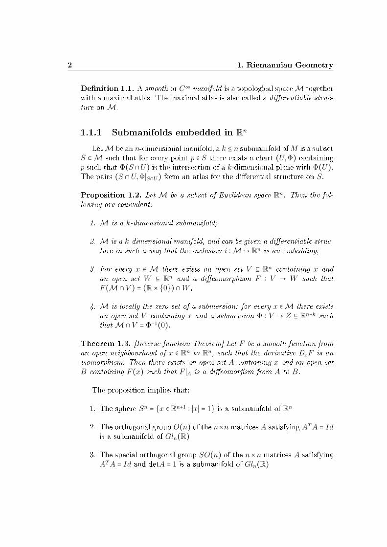
Proposition 1.2. Let M be a subset of Euclidean space Rn. Then the fol-lowing are equivalent:
1. M is a k-dimensional submanifold;
2. M is a k-dimensional manifold, and can be given a dierentiable struc-ture in such a way that the inclusion i ∶M Rn is an embedding;
3. For every x ∈ M there exists an open set V ⊆ Rn containing x andan open set W ⊆ Rn and a dieomorphism F ∶ V → W such thatF (M ∩ V ) = (R × 0) ∩W ;
4. M is locally the zero set of a submersion: for every x ∈M there existsan open set V containing x and a submersion Φ ∶ V → Z ⊆ Rn−k suchthat M ∩ V = Φ−1(0).
Theorem 1.3. [Inverse function Theorem] Let F be a smooth function froman open neighbourhood of x ∈ Rn to Rn, such that the derivative DxF is anisomorphism. Then there exists an open set A containing x and an open setB containing F (x) such that F ∣A is a dieomorsm from A to B.
The proposition implies that:
1. The sphere Sn = x ∈ Rn+1 ∶ ∣x∣ = 1 is a submanifold of Rn
2. The orthogonal group O(n) of the n×n matrices A satisfying ATA = Idis a submanifold of Gln(R)
3. The special orthogonal group SO(n) of the n×n matrices A satisfyingATA = Id and detA = 1 is a submanifold of Gln(R)
1.1 Smooth Manifolds 3
1.1.2 Tangent space
LetM a manifold and p ∈M, it is possible to dene the notion of tangentspace at this point.
Denition 1.4. Let p ∈M be any point of the n-dimensional manifoldM,given two C1-curves γ1 ∶] − ε, ε[→ M and γ2 ∶] − ε, ε[→ M passing throughp (i.e. γ1(0) = γ2(0) = p ) are equivalent if and only if there is some chart(U,Φ) at p such that:
(Φ γ1)′(0) = (Φ γ2)′(0)
Denition 1.5 (Tangent Vectors). Given a manifold M for any p ∈ M atangent vector to M at p is any equivalence class of C1−curves through p onM, modulo the equivalence relation dened on denition 1.4. The set of alltangent vectors at p is denoted by Tp(M):
TpM = γ ∶ (−ε, ε)→M s.t.γ(0) = p / ∼
Denition 1.6. A smooth vector eld X on a manifoldM is a linear mapX ∶ C∞(M)→ C∞(M) such that:
X(fg) = fX(g) + gX(f) ∀f, g ∈ C∞(M)
1.1.3 Ane Connection on Smooth Manifolds
The main obstacle to the denition of dierential of a vector eld X, isthat for every point p, q, X(p) and X(q) belong to the tangent space to themanifoldM at dierent points and can not be subtracted. It is necessary tointroduce the notion of ane connection.
Denition 1.7. Let M be a smooth manifold, an ane connection on Mis a dierential operator, send smooth vector elds X and Y to a smoothvector eld ∇XY :
∇ ∶ C∞(M, TM) × C∞(M, TM)→ C∞(M, TM)(X,Y )↦ ∇XY
which satises for all smooth vector elds X,Y and Z and real-vaued func-tions f onM:
1. ∇X+YZ = ∇XZ +∇YZ
4 1. Riemannian Geometry
2. ∇fXY = f∇XY
3. ∇X(Y +Z) = ∇XY +∇XZ
4. ∇X(fY ) =X[f]Y + f∇XY
The vector eld ∇XY is known as the covariant derivative of the vectoreld Y along X (with respect to the connection). The torsion tensor T ofan ane connection ∇ is the operators sending smooth vector elds X andY onM to the smooth vector elds T (X,Y ) given by:
T (X,Y ) = ∇XY −∇YX − [X,Y ]where [X,Y ](f) =XY (f) − Y X(f) for all f real-valued function.If the manifold is equipped with an ane connection, then this connectionallows one to transport vectors of the manifold along curves so that theystay parallel with respect to the connection, this idea is at the basis of thedenition of parallel transport which is about to be introduced.
Remark 1.8. An ane connection ∇ on M is said to be torsion-free if itstorsion tensor is everywhere zero, so that ∇XY −∇YX = [X,Y ] for all smoothvector elds X and Y onMDenition 1.9. If γ ∶ [a, b] → M is a smooth curve and ξ ∈ TxM, wherex = γ(a), then a vector eld X along γ (and in particular, the value of thisvector eld at y = γ(b)) is called the parallel transport of ξ along γ if
1. ∇γ(t)X = 0∀ t ∈ [a, b]
2. Xγ(a) = ξIt is necessary to dene the covariant derivative, before giving the deni-
tion of geodesic:
Denition 1.10. A smooth vector eld along the curve γ ∶ I → M is asmooth map V ∶ I → TM such that V (t) ∈ Tγ(t)M for all t ∈ I. It is calledT (γ) the space of the smooth vector eld along γ.A connection ∇ on the manifold M denes an unique operator for everycurves γ ∶ I →M:
Dt ∶ T (γ)→ T (γ)such that:
1. Dt is linear on R: Dt(aV + bW ) = aDtV + bDtW ∀a, b ∈ R
2. Dt satisfy: Dt(fV ) = fV + fDtV ∀ f ∈ C∞(I)Denition 1.11. Let ∇ be a connection on a manifoldM and let γ ∶ I →Ma curve onM. It is said that γ s a geodesic for ∇ if and only if
Dtγ ≡ 0

1.2 Riemannian Manifolds 5
1.2 Riemannian Manifolds
Denition 1.12. A Riemannian Metric on a dierentiable manifold M isgiven by a scalar product on each tangent space TpM which depends C∞ onthe base point p ∈M. A Riemannian manifold is a dierentiable manifold,equipped with a Riemannian metric.
In local coordinates, a metric is represented by a positive denite, sym-metric matrix called local representation of the Riemannnian metric in thechart x:
(gij(x))i,j=1,⋯,n
dened onM.
The product of two tangent vectors v,w ∈ TpM with coordinate represen-tations (v1, ..., vn) and (w1, ....,wn) respectively, is:
< v,w >g= gij(x(p))viwj
In particular, < ∂∂xi, ∂∂xj
>= gij, where ∂∂xi
is a base of the tangent space TpM.
The length of of v is given by ∣∣v∣∣ =< v, v > 12 .
Theorem 1.13. Each dierentiable manifold may be equipped with a Rie-mannian metric.
Proof. see [4]
1.2.1 Riemmanian distance and geodesics
Given a regular curve γ, the norm of its derivative is well dened andallows to dene the length of the curve:
Denition 1.14. Let (M, g) be a connected manifold. The length on themetric g of a smooth curve γ ∶ [a, b]→M is the following:
L(γ) = ∫b
a∥ ˙γ(t)∥
gdt = ∫
b
a(< ˙γ(t), ˙γ(t) >γ(t))
12dt
In local coordinate x = (x1(γ(t)), ..., xn(γ(t))):
L(γ) = ∫b
a
√gij(x(γ(t))
dxi
dt(γ(t))dx
j
dt(γ(t))dt
6 1. Riemannian Geometry
Denition 1.15. Let M be a connected manifold and p, q ∈M. Let ⟨., .⟩gbe a Riemannian metric onM. The distance between two points p and q isdened as:
dg(p, q) ∶= inf L(γ) ∣γ ∶[a, b ]→M piecewise smooth curves withγ(a) = p, γ(b) = q
Lemma 1.16. The distance function satises the axioms:
1. dg(p, q) ≥ 0 ∀p, q ∈M;dg(p, q) = 0⇔ p = q;
2. dg(p, q) = dg(q, p);
3. dg(p, q) ≤ dg(p, r) + dg(r, q) ∀p, q, r ∈M.
Proof. The proof is shown in [4].
Denition 1.17. The curves realizing the minimum of the Riemannian dis-tance for any two points of the manifold are called minimizing geodesics.
Denition 1.18. The manifold is said geodesically complete if any geodesiccan be dened on the whole R:
γ ∶ R→M
If a manifold is geodesically complete, it has no boundary nor any singularpoint that can be reached in a nite time.
Theorem 1.19 (Hopf-Rinow-De Rham theorem). Let M be a connectedRiemannian manifold. Then the following statements are equivalent:
M is a complete metric space
The closed and bounded subset of M are compact
M is geodesically complete
Furthermore, this theorem implies that given any two points p and q inM, there exists a length minimizing geodesic connecting these two points.

1.3 The Levi-Civita Connection 7
1.3 The Levi-Civita Connection
Let (M, g) be a Riemannian manifold and let ∇ be an ane connectiononM. It is said that ∇ is compatible with the Riemannian metric g if:
Z[g(X,Y )] = g(∇ZX,Y ) + g(X,∇ZY )
for all smooth vector eldsX,Y and Z onM. On every Riemannian manifoldthere exists a unique torsion-free connection that is compatible with theRiemannian metric.
Theorem 1.20. Let (M, g) be a Riemannian manifold. Then there exists aunique torsion-free ane connection ∇ on M compatible with the Rieman-nian metric g. This connection is characterized by the identity:
2g(∇XY,Z) =X[g(Y,Z)] + Y [g(X,Z)] −Z[g(X,Y )]++g([X,Y ]Z) − g([X,Z], y) − g([Y,Z],X)
for all smooth vector elds X,Y and Z on M.
Proof. The proof is shown in [19]
It is known as Levi-Civita connection. The geodesics computed withrespect to this connection are called Riemannian geodesics.
Denition 1.21. Let (M, g) be a Riemannian manifold of dimension n, andlet γ ∶ I →M be a smooth curve inM, dened over some interval I in R. γis a Riemannian geodesic if and only if
Dt (dγ(t)dt
) = 0 (1.1)
Denition 1.22. Given a chart (x1,⋯, xn) over some open set U ∈M, theChristoel symbols are dened:
Γijk =1
2gim(∂kgmj + ∂jgmk − ∂mgjk)
where (gij) = (gij)−1 is the inverse of the metric matrix.
The Levi-Civita connection is determined in a local system through theChristoel symbols:
∇∂j∂k =n
∑i=1
Γijk∂i (1.2)
then Γijk = Γikj.
8 1. Riemannian Geometry
Let γ ∶ I → U be a smooth curve in U , and let γi(t) = xi γ(t) for allt ∈ γ−1(U).Then
dγ(t)dt
=n
∑k=1
dγk(t)dt
∂k
So that:
D
dt
dγ(t)dt
=n
∑k=1
(d2γk(t)dt2
∂k +dγk(t)dt
n
∑j=1
dγj(t)dt
∇∂j∂k)
=n
∑i=1
(d2γi(t)dt2
+n
∑j=1
n
∑k=1
Γijk(γ(t))dγj(t)dt
dγk(t)dt
)∂i
So γ ∶ I → U is a geodesic if and only if:
d2γi(t)dt2
+n
∑j=1
n
∑k=1
Γijk(γ(t))dγj(t)dt
dγk(t)dt
= 0 i = 1,⋯, n (1.3)
Next theorem ensures that geodesics dened by means of the connection,are indeed minimizing geodesics in the sense of denition 1.17 above if andonly if the connection is compatible with the Riemannian metric.
Theorem 1.23. Let p and q be distinct points in a Riemannian manifold(M, g) and let γ ∶ [a, b] →M be a piecewise smooth curve in M from p toq, parametrized by the arclength. Suppose that the length of γ is less than orequal to the length of every other piecewise smooth curve from p to q. Thenγ is a smooth geodesic in M.
Proof. The proof of this theorem can be viewed in [19].
It is shown that the geodesics in the sphere Sn are the great circle.
Example 1.24 (Sphere S2). The Riemannian metric on the sphere is inducedby the embedded space R3, indeed the more simple Riemannian metric isthe Euclidean metric, which metric matrix is the identity g = Id or can alsowritten in Cartesian coordinates by g = dx2 + dy2 + dz2.It is chosen spherical coordinates on the sphere S2 ⊂ R3:
⎧⎪⎪⎪⎪⎨⎪⎪⎪⎪⎩
x = R sinφ cos θ
y = R sinφ sin θ
z = R cosφ
(1.4)
1.3 The Levi-Civita Connection 9
where θ ∈ (−π,π) and φ ∈ (0, π), while R is the radius of the sphere.Computing dx,dy and dz in spherical coordinates, it is found:
⎧⎪⎪⎪⎪⎨⎪⎪⎪⎪⎩
dx = R(φ′ cosφ cos θ − θ′ sinφ sin θ)dy = R(φ′ cosφ sin θ + θ′ sinφ cos θ)dz = Rφ′ sinφ
(1.5)
Hence, the metric on the sphere is:
gsphere = R2dφ2 +R2 sin2 φdθ2
So the metric matrix is:
gsphere = (R2 0
0 R2 sin2 φ) (1.6)
Formula 1.3 can be applied to compute geodesics. So that the computationof the Christoel symbols is necessary. By denition 1.22:
Γθφθ =(∂φgθφ + ∂θgφφ − ∂φgφθ)gφθ
2+ (∂φgθθ + ∂θgφθ − ∂θgφθ)gθθ
2
= ∂φ(R2 sinφ) 1
2R2 sin2 φ= cosφ
sinφ= arctanφ
Γφθθ =(∂θgθφ + ∂θgθφ − ∂φgθθ)gφφ
2+ (∂θgθθ + ∂θgθθ − ∂θgθθ)gθφ
2
= ∂φ(R2 sinφ) 1
2R2= − sinφ cosφ
Γθθθ =(∂θgθθ)gθθ
2= 0
The other Christoel symbols are zero Γθθθ = Γθφφ = Γφθθ = Γφφφ = 0.Then, the geodesics are the curves γ(t) = (θ(t), φ(t)) that satisfy that dier-ential equation:
⎧⎪⎪⎨⎪⎪⎩
φ − θ2 sinφ cosφ = 0
θ + φθ arctanφ = 0(1.7)
Since the meridians are dened by φ = θ = θ = 0, and they satisfy thesystem above, it can be claimed that the meridians are geodesics.
Proposition 1.25. The geodesics on a sphere are the arcs from great circles,that is, arcs from circles formed by the intersection of a plane containing thecenter of the sphere with the sphere itself.

10 1. Riemannian Geometry
1.3.1 Exponential and Logarithmic map
Formula 1.3 and standard existence and uniqueness theorems for solutionsof ordinary dierential systems of equations ensure that, given a tangentvector ∂v ∈ TxM at any point x ∈M and given any real number t0, existsa unique maximal geodesic γ ∶ I → M dened on some open interval Icontaining t0, such that γ(t0) = x and γ′(to) = ∂v. Moreover exists δx > 0such that it can be dened the exponential map as:
expx ∶ ∂v ∈ TxM ∶ ∣∂v ∣ < δx→M
at x is dened by expx(∂v) = γ(x,∂v)(1) .
A corollary of the Hopf-Rinow De Rham Theorem 1.19 can be stated asfollows:
Corollary 1.26. Let (M, g) be a connected Riemannian manifold. Then thefollowing three conditions are equivalent:
1. the Riemannian distance function onM is complete (i.e. every Cauchysequence in M converges);
2. the Riemannian manifold (M, g) is geodesically complete;
3. there exists a point p onM with the property that the exponential mapexpp is dened over the whole tangent space TpM toM at p (i.e. everygeodesic passing through the point p can be extended to a geodesic fromR into M)
Then the exponential map is dened in the whole tangent space:
expx ∶ TxM→M (1.8)
∂v ↦ expx(∂v) = γ(x,∂v)(1) (1.9)
The exponential is a local dieomorphism and its inverse is the logarithmicmap denoted by
→pq= Logp(q), this is the smallest vector (in norm) such that
q = expp(→pq).
Logp ∶M→ TpMq ↦ →pq= Logp(q)
In this chart the geodesics going through p are represented by the linesgoing through the origin Logpγ(p,→pq)(t) = t
→pq.
1.3 The Levi-Civita Connection 11
Since the exponential map is a local dieomorphism, the distance denedon the manifold is locally equivalent to a norm dened on the tangent plane.Indeed there exist c1, c2 constants such that, for all q = expp(v), satisfy:
c1∥v∥ ≤ d(p, q) ≤ c2∥v∥Example 1.27 (Sphere). Given two points on the sphere p and q ∈ Sn, whichare parametrized by the vectors starting from the origin o: p = →op q =→oq. Thedistance induced from the metric is d(p, q) = arccos(pT q) = θ ∈ [0, π].Given x ∈ Sn and v ∈ TxSn such that ∥v∥ = 1. The curve γv(t) = cos(t)x +sin(t)v is the only geodesic which satisfy γv(0) = x and γ′v(0) = v. Then fromthe denition the exponential map:
expx ∶ TxSn → Sn
v → γv(1)Therefore expx(v) = cos(∣v∣)x + sin(∣v∣)v.The inverse is the Logarithmic map:
Logx ∶ Sn → TxSn
y → θ
sin θ(y − cos(θ)x)
1.3.2 Cut Locus
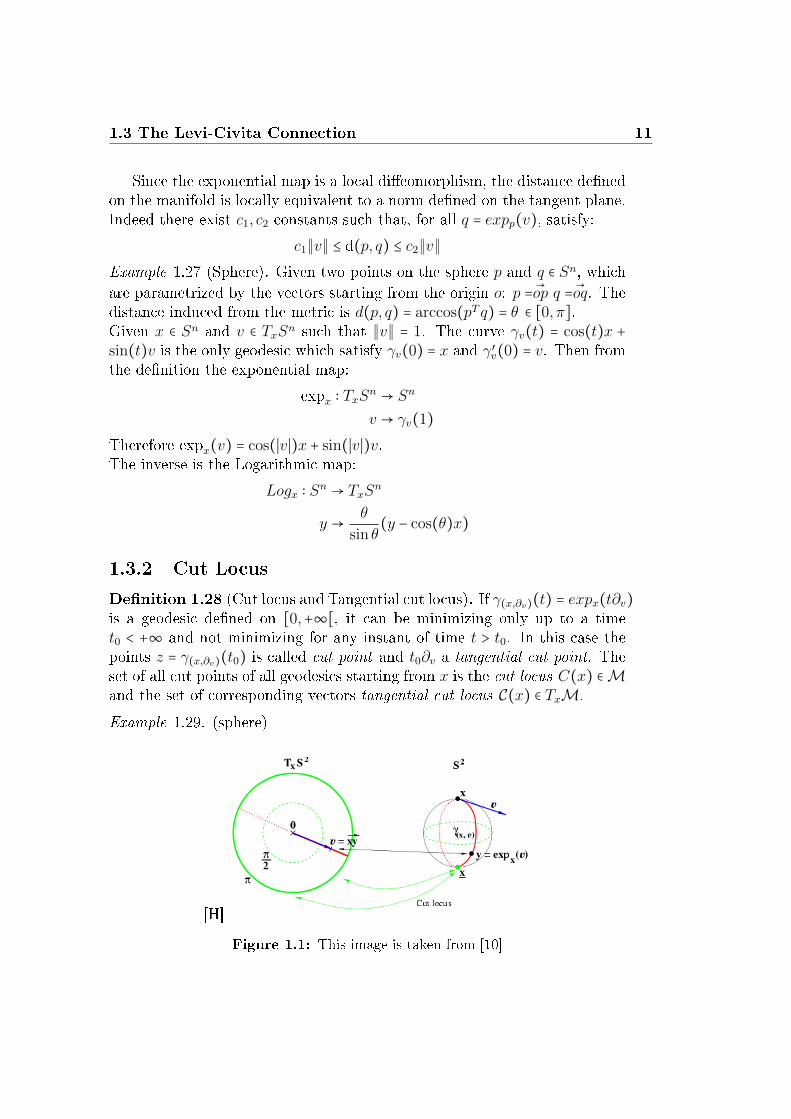
Denition 1.28 (Cut locus and Tangential cut locus). If γ(x,∂v)(t) = expx(t∂v)is a geodesic dened on [0,+∞[, it can be minimizing only up to a timet0 < +∞ and not minimizing for any instant of time t > t0. In this case thepoints z = γ(x,∂v)(t0) is called cut point and t0∂v a tangential cut point. Theset of all cut points of all geodesics starting from x is the cut locus C(x) ∈Mand the set of corresponding vectors tangential cut locus C(x) ∈ TxM.
Example 1.29. (sphere)
[H]
Figure 1.1: This image is taken from [10]
12 1. Riemannian Geometry
In the sphere the cut locus of a point p is its antipodal point −p
1.4 Lie Groups
Denition 1.30. A Lie Group is a smooth manifold G which is also a groupsuch that the two group operations, multiplication and inverse, are smoothmaps.
m ∶ G ×G→ G ∈ C∞ i ∶ G→ G ∈ C∞
(g, h)→ gh g → g−1
Denition 1.31. A map F ∶ H → G between two Lie groups H and G is aLie group homonorphism if it is a smooth map and a group homomorphism.
The group of homomorphism condition means that for all h,x ∈ H:F (hx) = F (h)F (x). This can be written using the left multiplication whichis the dieomorphism `a ∶ G → G for an element a in a Lie group G, in thefollowing way: F `h = `F (h) F for all h ∈H.The general denition of Lie algebra is given by:
Denition 1.32. Let K be a eld. A vector space g over K is called LieAlgebra if there exists:
[ , ] ∶ g × g→ g
with the following properties X,Y,Z ∈ g:
[X,Y ] = − [Y,X]
Jacobi identity: [X [Y,Z]] + [Y [Z,X]] + [Z, [X,Y ]]
Since the left translation of a Lie group G by an element g ∈ G is a dieo-morphism that maps a neighborhood of the identity to a neighborhood of g,all the local information about the group is concentrated in a neighborhoodof the identity.Moreover, on the tangent space TeG can be given a Lie bracket [, ], so itbecomes a Lie algebra of the Lie group.The Lie bracket on the tangent space TeG is dened using the canonical iso-morphism between the tangent space at the identity and the vector space ofthe left invariant vector elds on G:
Denition 1.33. Let G Lie Group and X ∈ X(G) a vector eld, X is saidleft invariant if
d`gX =X `g
1.4 Lie Groups 13
where `g ∶ G→ Gh↦ gh.The Lie Algebra of the Lie Group is dened as:
Lie(G) = g = X ∈X(G)∣d`gX =X `g
Theorem 1.34 (Von Neumann Theorem). Let G be a real algebraic group.Then G is a closed real Lie subgroup of Gl(n,R)
Example 1.35. This Theorem implies that:
1. Sln(R)
2. SO(n)
3. O(n)
are Lie subgroups in GlnR
Theorem 1.36. There is a vector space isomorphism between:
Lie (G)↔ Te(G)X ↦Xe
A A
Proof. A complete proof is shown in [16].
Using this theorem, in groups we can dene a group exponential map,analogous to the one dened in 1.8 , but with values on the algebra insteadof the tangent plane.
1.4.1 Group Exponential map
Firstly, we need the following theorem to dene the one-parameter sub-groups:
Theorem 1.37. Let G and H be two Lie groups with Lie algebras g andh respectively and G simply connected. Let Ψ ∶ g → h be a homomorphism.Then there exists a unique homomorphism Φ ∶ G→H such that dΦ = Ψ.
Proof. In [18].
Denition 1.38. Let G be a Lie Group a one-parameter subgroup is a ho-momorphism of Lie group α ∶ R→ G
14 1. Riemannian Geometry
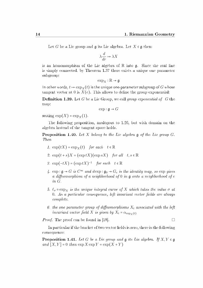
Let G be a Lie group and g its Lie algebra. Let X ∈ g then:
λd
dr↦ λX
is an homomorphism of the Lie algebra of R into g. Since the real lineis simply connected, by Theorem 1.37 there exists a unique one parametersubgroup:
expX ∶ R→ g
In other words, t↦ expX(t) is the unique one-parameter subgroup ofG whosetangent vector at 0 is X(e). This allows to dene the group exponential:
Denition 1.39. Let G be a Lie Group, we call group exponential of G themap:
exp ∶ g→ G
setting exp(X) = expX(1).The following proposition, analogous to 1.26, but with domain on the
algebra instead of the tangent space holds.
Proposition 1.40. Let X belong to the Lie algebra g of the Lie group G.Then
1. exp(tX) = expX(t) for each t ∈ R
2. exp(t + s)X = (exp tX)(exp sX) for all t, s ∈ R
3. exp(−tX) = (exp tX)−1 for each t ∈ R
4. exp ∶ g→ G is C∞ and d exp ∶ g0 → Ge is the identity map, so exp givesa dieomorphism of a neighborhood of 0 in g onto a neighborhood of ein G.
5. `σ expX is the unique integral curve of X which takes the value σ at0. As a particular consequence, left invariant vector elds are alwayscomplete.
6. the one-parameter group of dieomorphisms Xt associated with the leftinvariant vector eld X is given by Xt = αexpX(t)
Proof. The proof can be found in [18].
In particular if the bracket of two vector elds is zero, there is the followingconsequence:
Proposition 1.41. Let G be a Lie group and g its Lie algebra. If X,Y ∈ gand [X,Y ] = 0 then expX expY = exp(X + Y )
1.4 Lie Groups 15
1.4.2 Baker-Campbell-Hausdor Formula
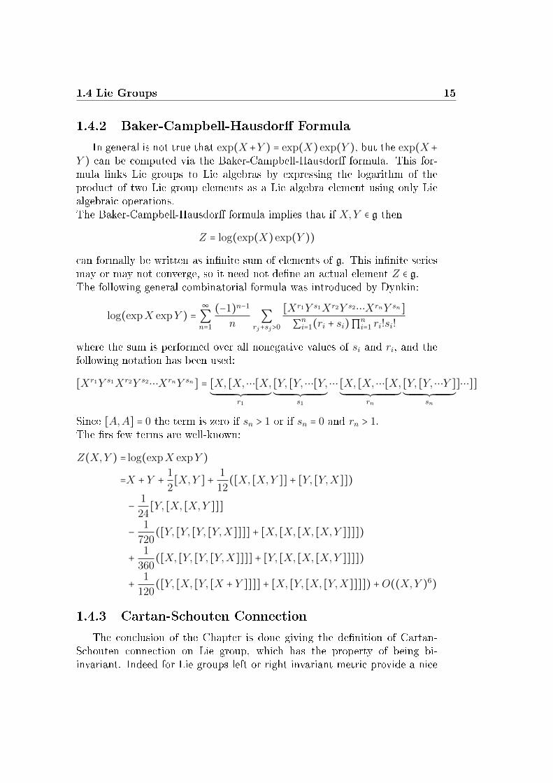
In general is not true that exp(X +Y ) = exp(X) exp(Y ), but the exp(X +Y ) can be computed via the Baker-Campbell-Hausdor formula. This for-mula links Lie groups to Lie algebras by expressing the logarithm of theproduct of two Lie group elements as a Lie algebra element using only Liealgebraic operations.The Baker-Campbell-Hausdor formula implies that if X,Y ∈ g then
Z = log(exp(X) exp(Y ))
can formally be written as innite sum of elements of g. This innite seriesmay or may not converge, so it need not dene an actual element Z ∈ g.The following general combinatorial formula was introduced by Dynkin:
log(expX expY ) =∞∑n=1
(−1)n−1
n∑
rj+sj>0
[Xr1Y s1Xr2Y s2⋯XrnY sn]∑ni=1(ri + si)∏n
i=1 ri!si!
where the sum is performed over all nonegative values of si and ri, and thefollowing notation has been used:
[Xr1Y s1Xr2Y s2⋯XrnY sn] = [X, [X,⋯[X,´¹¹¹¹¹¹¹¹¹¹¹¹¹¹¹¹¹¹¹¹¹¹¹¹¹¹¹¹¹¹¹¸¹¹¹¹¹¹¹¹¹¹¹¹¹¹¹¹¹¹¹¹¹¹¹¹¹¹¹¹¹¹¹
r1
[Y, [Y,⋯[Y,´¹¹¹¹¹¹¹¹¹¹¹¹¹¹¹¹¹¹¹¹¹¹¹¹¹¸¹¹¹¹¹¹¹¹¹¹¹¹¹¹¹¹¹¹¹¹¹¹¹¹¹
s1
⋯ [X, [X,⋯[X,´¹¹¹¹¹¹¹¹¹¹¹¹¹¹¹¹¹¹¹¹¹¹¹¹¹¹¹¹¹¹¹¸¹¹¹¹¹¹¹¹¹¹¹¹¹¹¹¹¹¹¹¹¹¹¹¹¹¹¹¹¹¹¹
rn
[Y, [Y,⋯Y ]´¹¹¹¹¹¹¹¹¹¹¹¹¹¹¹¹¹¹¹¹¹¹¹¹¸¹¹¹¹¹¹¹¹¹¹¹¹¹¹¹¹¹¹¹¹¹¹¹¹
sn
]⋯]]
Since [A,A] = 0 the term is zero if sn > 1 or if sn = 0 and rn > 1.The rs few terms are well-known:
Z(X,Y ) = log(expX expY )
=X + Y + 1
2[X,Y ] + 1
12([X, [X,Y ]] + [Y, [Y,X]])
− 1
24[Y, [X, [X,Y ]]]
− 1
720([Y, [Y, [Y, [Y,X]]]] + [X, [X, [X, [X,Y ]]]])
+ 1
360([X, [Y, [Y, [Y,X]]]] + [Y, [X, [X, [X,Y ]]]])
+ 1
120([Y, [X, [Y, [X + Y ]]]] + [X, [Y, [X, [Y,X]]]]) +O((X,Y )6)
1.4.3 Cartan-Schouten Connection
The conclusion of the Chapter is done giving the denition of Cartan-Schouten connection on Lie group, which has the property of being bi-invariant. Indeed for Lie groups left or right invariant metric provide a nice

16 1. Riemannian Geometry
setting as the Lie group becomes a geodesically complete Riemannian mani-fold, thus also metrically complete. This Riemannian approach is fully con-sistent with the group operations only if a bi-invariant metric exists. Moredetails are shown in [8].
Denition 1.42. For any vector elds X and Y and any group elementg ∈ G we say that a connection is a left invariant connection if satises∇d`gX
d`gY = d`g∇XY
Denition 1.43. Among the left invariant connections, the Cartan-Schoutenconnections are the ones for which geodesics going through identity are one-parametry subgroups. Bi-invariant connections are both left and right in-variant.
Theorem 1.44. Cartan-Schouten connections are uniquely determined bythe property α(x,x) = 0 for all x ∈ g where α ∶ g × g→ g.Bi-invariant connections are characterizeed by the condition:
α([z, x], y) + α(x, [z, y]) = [z,α(x, y)] ∀x, y, z ∈ g
The one dimensonal family of connections generated by α(x, y) = λ[x, y]satisfy these two conditions. Moreover, there is a unique symmetric Cartan-Schouten bi-invariant connection called the canonical connection of the Liegroup (also called mean or 0−connection) dened by α(x, y) = 1
2[x, y] for allx, y ∈ g i.e. ∇X Y = 1
2[X, Y ] for two left-invariant vector elds.

Chapter 2
Statistics on Riemmannian
Manifolds
The purpose of this chapter is to dene the statistics which are needed toexplain Barycentric Subspaces. In this studies the data lie on a known man-ifold, and the goal is to study statistics of data restricted to this manifold.Then the statistical computing on manifolds is a domain in which dierentialgeometry meets statistics.Information about probability theory is taken from Pennec [10].
Firstly the denition of probability space has to be transferred on a Rie-mannian manifold. For doing that it is needed a denition of measure onthe manifold and this is induced by the Riemannian metric, i.e. by theinnitesimal volume element on each tangent space:
Denition 2.1. The volume element in n-dimensional Riemannian manifoldwith metric G(x) = [gij(x)] is dened by the following formula:
dM(x) =√
∣detG(x)∣dx
Let (Ω,B(Ω),P) be a probability space where Ω is the whole space of theevents, B(Ω) is the σ-algebra of Borel, i.e. the smallest σ-algebra containingall the open subsets of Ω and P ∶ B(Ω) → [0,1] is a probability measure, i.e.P(Ω) = 1 and it has to satisfy Kolmogorov's axioms.
Denition 2.2. A random point in the Riemannian manifoldM is a Borelmeasurable function X =X(w) from Ω toM.
The induced measure is P X−1. In particular, take
X ∶ (Ω,B,P)→ (M,A)
17

18 2. Statistics on Riemmannian Manifolds
where A is the σ−algebra onM.
It is important to dene the probability of an event occurring, this de-pends on its distribution. This can be given by its distribution function, byits probability mass function (if the variables are discrete) or by probabilitydensity function (if the variables are continuous). So in case the variables arecontinuous, denoting the probability of an event χ occurring by P(X ∈ χ):
Denition 2.3. Let A be the Borel σ−algebra ofM. The random point Xhas probability density function pX (real positive and integrable function) if:
∀χ ∈ A P(X ∈ χ)∫χp(y)dM(y) P(X ∈M) = ∫
Mp(y)dM(y) = 1
Since the cut locus has null measure it is possible to integrate on M inan exponential chart.If f is an integrable function of the manifold and fp(
→pq) = f(expp(
→pq)) is its
image in the exponential chart at p, we have:
∫Mf(p)dM = ∫
D(p)fp(
→z)
√G→x(→z)d →z
2.1 Expected value of a function
One of the main concept to dene in statistic is the expected value, i.e. therst moment of a distribution. Moments are really important to distinguishone distribution from another.Let φ(X(w)) be a Borelian real valued function dened on M and χ arandom point of pdf fx. Then φ(χ) is a real random variable and we cancompute its expectation:
E[φ(X)] = ∫Mφ(y)pX(y)dM(y)
2.2 Variance
The second moment of a distribution is the variance, or the square of thestandard deviation, which is very important in statistic because it measuresthe spread of the data
σ2X(y) = E[dist(y,X)2] = ∫
Mdist(y, z)2pX(z)dM(z)

2.3 Fréchet expectation 19
2.3 Fréchet expectation
One of the most interesting denition of expected value for geodesicallycomplete Riemannian manifolds is the Fréchet and Karcher expectation. Itis important to notice that the denition can be used in metric space, whichare denitly more general than manifolds.
Denition 2.4 (Fréchet expectation). Let X be a random point. If thevariance σ2
X(y) is nite for all point y ∈ M, every point minimizing thisvariance is called expected or mean point. Thus, the set of mean points is:
E[X] = argminy∈M
(E[dist(y,X)2])
if there exists a least one mean point x, it is called variance the minimalvalue σ2
X = σ2X(x).
In case of a set of discrete measures X1,⋯,Xn the empirical or discretemean points :
E[Xi] = argminy∈M
(E[dist(y,Xi)2]) = argminy∈M
( 1
n∑i
dist(y,Xi)2)
So the Fréchet are the set of points minimizing globally the variance, whileKarcher proposed to consider the local minima. Thus, the Fréchet mean arethe subset of the Karcher ones.
2.3.1 Metric power of Fréchet expectation
The Fréchet (resp. Karcher) mean can be further generalized by takinga power α of the metric dene the α−variance.
σX,α(y) = (E[dist(y,X)α]) 1α = (∫
Mdist(y, z)αpX(z)dM(z))
1α
In case of measures X1,⋯,Xn the empirical or discrete mean point :
σX,α(y) = (E[dist(y,X)α]) 1α = ( 1
n∑i
distα(y,Xi))1α
The global minima of the α−variance denes the Fréchet median for α = 1, theFréchet mean for α = 2 and the barycenter of the support of the distributionfor α =∞.

20 2. Statistics on Riemmannian Manifolds

Chapter 3
Barycentric Subspace Analysis
A powerful tool for multivariate statistical analysis is principal compo-nent analysis (PCA), which is very important to reduce the dimensionalityof the data and yields a hierarchy of major directions explaining the mainsources of data variation. The problem arise when multivariate data lies ina non-Euclidean space, such as Riemannian structure. Then it is needed togeneralize this tool.In this chapter it is introduced the denition of Barycentric Subspace, whichwas rst introduced by X. Pennec (2015) and it is a generalization of theconcept of ane subspace in Euclidean space. Depending on the generaliza-tion of the mean that is used on the manifold: Fréchet and Karcher meanor exponential barycenter, it is obtained the Fréchet/Karcher subspaces orthe ane span. These three denitions are related. Barycentric SubspaceAnalysis (BSA) is then generalization of PCA done building a forward orbackward analysis of nested subspaces. All the information are taken from[7].
3.1 Barycentric Subspace
First of all, the setting of the work is a Riemannian manifold geodesicallycomplete. Then, since in a Riemannian manifold the Riemannian log anddistance functions are not smooth in the cut locus, it is necessary to give twodenitions for working on the manifold:
Denition 3.1. Let x0,⋯, xk ⊂M be a set of k + 1 ≤ n reference points inthe n dimensional Riemannian manifoldM and C(x0,⋯, xk) = ⋃ki=0 C(xi) bethe union of the cut loci of these points. It is called the smooth manifoldMand the k + 1 reference points a (k + 1)-pointed manifold. The submanifold
21
22 3. Barycentric Subspace Analysis
M∗(x0,⋯, xk) =M∖ C(x0,⋯, xk) of the non-cut points of the k + 1 referencepoints it is called (k + 1)-punctured manifold.
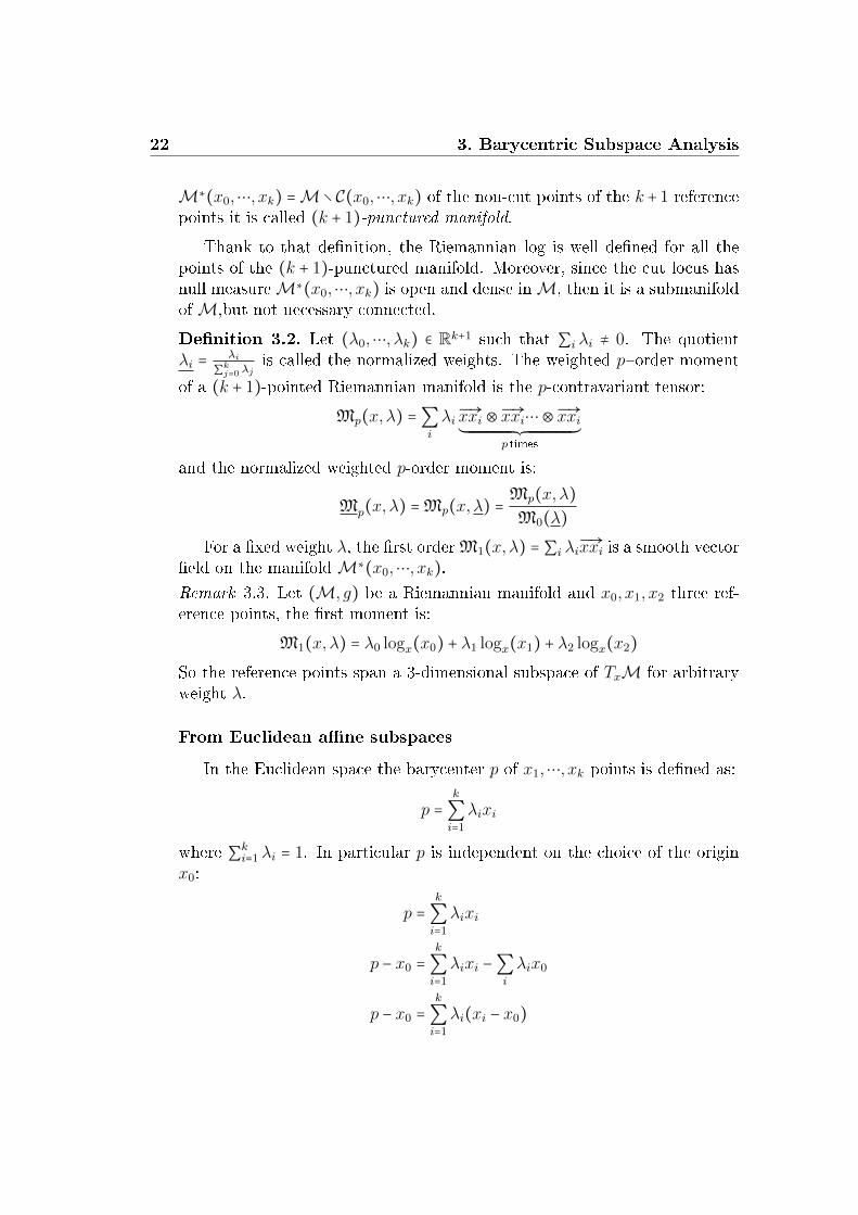
Thank to that denition, the Riemannian log is well dened for all thepoints of the (k + 1)-punctured manifold. Moreover, since the cut locus hasnull measureM∗(x0,⋯, xk) is open and dense inM, then it is a submanifoldofM,but not necessary connected.
Denition 3.2. Let (λ0,⋯, λk) ∈ Rk+1 such that ∑i λi ≠ 0. The quotientλi = λi
∑kj=0 λjis called the normalized weights. The weighted p−order moment
of a (k + 1)-pointed Riemannian manifold is the p-contravariant tensor:
Mp(x,λ) =∑i
λiÐ→xxi ⊗Ð→xxi⋯⊗Ð→xxi´¹¹¹¹¹¹¹¹¹¹¹¹¹¹¹¹¹¹¹¹¹¹¹¹¹¹¹¹¹¹¹¹¹¹¹¹¹¹¹¹¹¹¹¹¹¹¸¹¹¹¹¹¹¹¹¹¹¹¹¹¹¹¹¹¹¹¹¹¹¹¹¹¹¹¹¹¹¹¹¹¹¹¹¹¹¹¹¹¹¹¹¹¹
p times
and the normalized weighted p-order moment is:
Mp(x,λ) =Mp(x,λ) =Mp(x,λ)M0(λ)
For a xed weight λ, the rst orderM1(x,λ) = ∑i λiÐ→xxi is a smooth vector
eld on the manifoldM∗(x0,⋯, xk).Remark 3.3. Let (M, g) be a Riemannian manifold and x0, x1, x2 three ref-erence points, the rst moment is:
M1(x,λ) = λ0 logx(x0) + λ1 logx(x1) + λ2 logx(x2)So the reference points span a 3-dimensional subspace of TxM for arbitraryweight λ.
From Euclidean ane subspaces
In the Euclidean space the barycenter p of x1,⋯, xk points is dened as:
p =k
∑i=1
λixi
where ∑ki=1 λi = 1. In particular p is independent on the choice of the origin
x0:
p =k
∑i=1
λixi
p − x0 =k
∑i=1
λixi −∑i
λix0
p − x0 =k
∑i=1
λi(xi − x0)
3.1 Barycentric Subspace 23
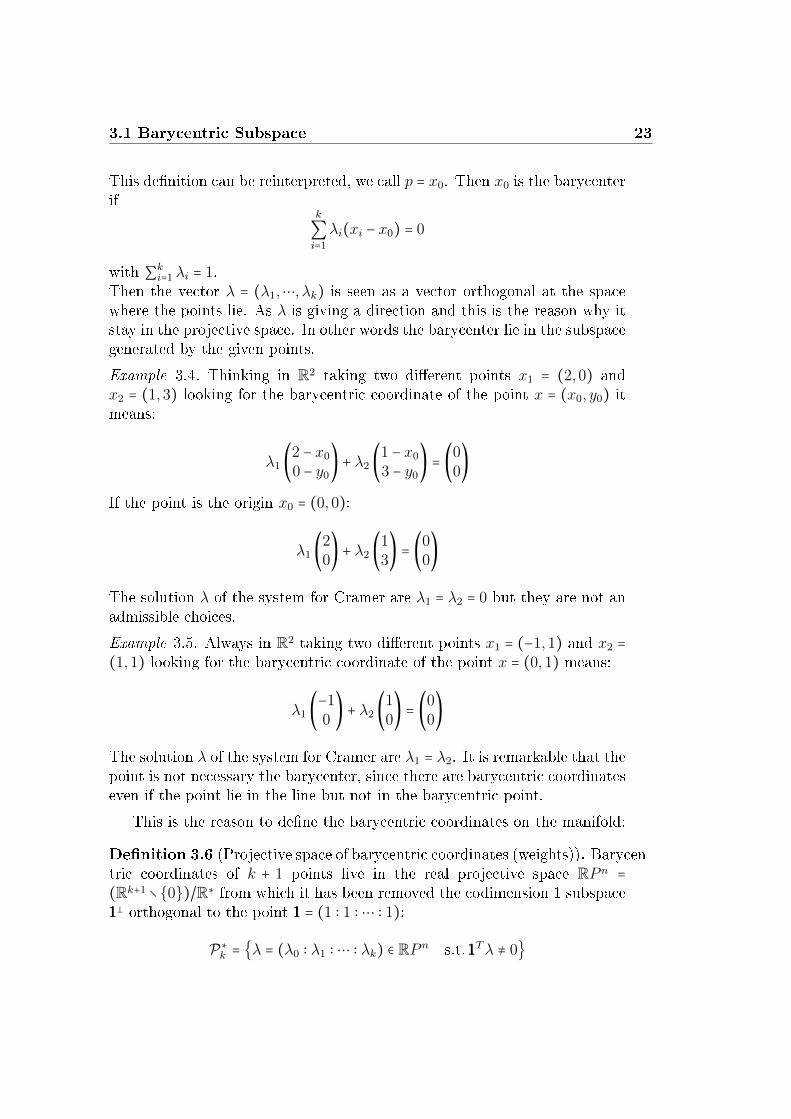
This denition can be reinterpreted, we call p = x0. Then x0 is the barycenterif
k
∑i=1
λi(xi − x0) = 0
with ∑ki=1 λi = 1.
Then the vector λ = (λ1,⋯, λk) is seen as a vector orthogonal at the spacewhere the points lie. As λ is giving a direction and this is the reason why itstay in the projective space. In other words the barycenter lie in the subspacegenerated by the given points.
Example 3.4. Thinking in R2 taking two dierent points x1 = (2,0) andx2 = (1,3) looking for the barycentric coordinate of the point x = (x0, y0) itmeans:
λ1 (2 − x0
0 − y0) + λ2 (
1 − x0
3 − y0) = (0
0)
If the point is the origin x0 = (0,0):
λ1 (20) + λ2 (
13) = (0
0)
The solution λ of the system for Cramer are λ1 = λ2 = 0 but they are not anadmissible choices.
Example 3.5. Always in R2 taking two dierent points x1 = (−1,1) and x2 =(1,1) looking for the barycentric coordinate of the point x = (0,1) means:
λ1 (−10) + λ2 (
10) = (0
0)
The solution λ of the system for Cramer are λ1 = λ2. It is remarkable that thepoint is not necessary the barycenter, since there are barycentric coordinateseven if the point lie in the line but not in the barycentric point.
This is the reason to dene the barycentric coordinates on the manifold:
Denition 3.6 (Projective space of barycentric coordinates (weights)). Barycen-tric coordinates of k + 1 points live in the real projective space RP n =(Rk+1∖0)/R∗ from which it has been removed the codimension 1 subspace111 orthogonal to the point 111 = (1 ∶ 1 ∶ ⋯ ∶ 1):
P∗k = λ = (λ0 ∶ λ1 ∶ ⋯ ∶ λk) ∈ RP n s.t.111Tλ ≠ 0
24 3. Barycentric Subspace Analysis
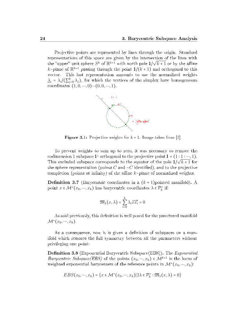
Projective points are represented by lines through the origin. Standardrepresentations of this space are given by the intersection of the lines withthe upper unit sphere Sk of Rk+1 with north pole 111/
√k + 1 or by the ane
k−plane of Rk+1 passing through the point 111/(k + 1) and orthogonal to thisvector. This last representation amounts to use the normalized weightsλi = λi/(∑k
j=0 λj), for which the vertices of the simplex have homogeneouscoordinates (1,0,⋯,0)⋯(0,0,⋯,1).
Figure 3.1: Projective weights for k = 1. Image taken from [7]
To prevent weights to sum up to zero, it was necessary to remove thecodimension 1 subspace 111 orthogonal to the projective point 111 = (1 ∶ 1 ∶ ⋯,1).This excluded subspace corresponds to the equator of the pole 111/
√k + 1 for
the sphere representation (points C and −C identied), and to the projectivecompletion (points at innity) of the ane k−plane of normalized weights.
Denition 3.7 (Barycentric coordinates in a (k + 1)pointed manifold). Apoint x ∈M∗(x0,⋯, xk) has barycentric coordinates λ ∈ P∗k if:
M1(x,λ) =k
∑i=0
λiÐ→xxi = 0
As said previously, this denition is well posed for the punctured manifoldM∗(x0,⋯, xk).
As a consequence, now it is given a denition of subspaces on a man-ifold which restores the full symmetry between all the parameters withoutprivileging one point:
Denition 3.8 (Exponential Barycentric Subspace(EBS)). The ExponentialBarycentric Subspace(EBS) of the points (x0,⋯, xk) ∈Mk+1 is the locus ofweighted exponential barycenters of the reference points inM∗(x0,⋯, xk):
EBS(x0,⋯, xk) = x ∈M∗(x0,⋯, xk)∣∃λ ∈ P∗k ∶M1(x,λ) = 0
3.1 Barycentric Subspace 25
In the following chapter it will be shown that in the sphere this denitionmeans to nd the great circle passing by the reference points. It was seen inthe Euclidean space that there were not a privileged points, and this is theproperty that we are looking for on a manifold, for instance in the sphere allthe points belonging to the subspace are the one in the great circle passingby the reference points, and then there are innite points that can be chosenas central points.
As a consequence, the space of admissible barycentric weights is
Λ(x) = λ ∈ P∗k ∣M1(x,λ) = 0
Proposition 3.9. x ∈ EBS(x0,⋯, xk) if and only if Λ(x) ≠ ∅
The discontinuity of the Riemannian log on the cut locus of the referencepoints may hide continuity or discontinuities of the exponential barycentricsubspace. Then for ensure the completeness and reconnect dierent compo-nents, it is considered the closure of this set:
Denition 3.10 (Ane span). The ane span is the closure of the Expo-nential Barycentric Subspace in M :
A(x0,⋯, xk) = EBS(x0,⋯, xk)
SinceM is geodesically complete, the metric completion of the EBS is guar-anteed.
The completeness of the ane span is fundamental because it allowsto always nd a closest point of the data on the subspace which is reallyimportant in the practice.
Example 3.11. In R2 taken two reference points x1 = (1,1) and x2 = (0,1),the EBS(x1, x2) = x ∈ R2∣∃λ ∈ P∗M1(x,λ) = 0.
λ1 (x − 1y − 1
) + λ2 (x − 0y − 1
) = (00)
Then: ⎧⎪⎪⎨⎪⎪⎩
λ1(x − 1) + λ2x = 0
λ2(y − 1) + λ2(y − 1) = 0
Solving the system for x and y:
⎧⎪⎪⎨⎪⎪⎩
λ1x − λ1 + λ2x = 0
λ2y − λ2 + λ2y − λ2 = 0
26 3. Barycentric Subspace Analysis
⎧⎪⎪⎨⎪⎪⎩
x = λ1λ1+λ2
y = 1
The solution is
EBS(x1, x2) = (x, y) ∈ R2∣( λ1
λ1 + λ2
,1)
Since, the setting is R2 the solution is the straight line passing through thetwo reference points, i.e. classical ane subspace in the Euclidean Space.
Let Z(x) = [ →xx0,⋯,→xxk] be the smooth eld of n × (k + 1) matrices of
vectors pointing from any point x ∈ M∗(x0,⋯, xk) to the reference points.
The constraint ∑i λi→xxi= 0 can be rewritten in matrix form M1(x,λ) =
Z(x)λ = 0 where λ is the k + 1 vector of homogeneous coordinates λi.A direct consequence of this statement is the following theorem:
Theorem 3.12. Let Z(x) = U(x)S(x)V (x)T be a singular decompositionof the n × (k + 1) matrix elds Z(x) = [ xx0,⋯, xxk] on M∗(x0,⋯, xk) withsingular values si(x)0≤i≤k sorted in decreasing order. EBS(x0,⋯, xk) is thezero levelset of the smallest singular value sk(x) and the dual subspace of validbarycentric weights is spanned by the right singular vectors corresponding tothe l vanishing singular values: Λ(x) = Span(vk−l,⋯, vk) (it is void if l = 0)
Proof. Following the paper [7]. Since U and V are orthogonal matrices,Z(x)λ = 0 if and only if at least one singular value (necessarily the smallestone sk) is null, and λ has to live in the corresponding right singular space:Λ(x) = Ker(Z(x)). If there is only one zero singular value (sk = 0 andsk−1 > 0), then λ is proportional to vk. If l singular values vanish, then thereis a higher dimensional linear subspace of solution for λ.
Example 3.13. Let consider in R5 the two points: x0 = (1,0,0,0,0) and x1 =
(0,1,0,0,0), then the matrix of them is Z(x) =
⎛⎜⎜⎜⎜⎜⎜⎝
1 00 10 00 00 0
⎞⎟⎟⎟⎟⎟⎟⎠
. The singular values
of Z(x) are the square root of the eigenvalues of Z(x)TZ(x) = (1 00 1
). Then
the solutions are s0 = s1 = 1 and the other are zero. Then s = diag(1,1,0,0,0).The theorem tells us that the subspace of valid barycentric weights is Λ(x) =Span(e3, e4, e5) and the EBS is the orthogonal e3 = e4 = e5.
3.1 Barycentric Subspace 27
Theorem 3.14. Let G(x) be the matrix expression of the Riemannian met-ric in a local coordinate system and Ω(x) = Z(x)TG(x)Z(x) be the smooth(k + 1) × (k + 1) matrix eld on M∗(x0,⋯, xk) with components Ωij(x) =<xxi, xxj > and Σ(x) = M2(x,1) = ∑k
i=0 xxixxiT = Z(x)Z(x)T be the (scaled)
n × n covariance matrix eld of the reference points. EBS(x0,⋯, xk) is thezero level set of det(Ω(x)), the minimal eigenvalue σ2
k+1 of Ω(x), the k + 1eigenvalue (in decreasing order) of the covariance Σ(x).
Proof. Following the proof from [7].The constraint M1(x,λ) = 0 is satised if and only if:
∥M1(x,λ)∥2x = ∥∑
i
λiÐ→xxi∥=xλT .Ω(x).λ = 0
As the function is homogeneous in λ, it can be restricted to unit vectors.Adding this constrains with a Lagrangian multiplier to the cost function, itis ended-up with the Lagrangian
L(x,λ,α) = λT .Ω(x).λ + α(λTλ − 1)
The minimum with respect to λ is obtained for the eigenvector µk+1(x) as-sociated to the smallest eigenvalue σk+1(x) of Ω(x) (assuming that eigenval-ues are sorted in decreasing order) and there is ∥M1(x,µk+1(x))∥2
2 = σk+1(x),which is null if and only if the minimal eigenvalue is zero. Thus, the barycen-tric subspace of k + 1 points is the locus of rank decient matrices Ω(x):
EBS(x0,⋯, xk) = φ−1(0) whereφ(x) = det(Ω(x))
One may want to relate the singular values of Z(x) to the eigenvalues ofΩ(x). The later are the square of the singular values of G(x)1/2Z(x). How-ever, the left multiplication by the square root of the metric (a non singularbut non orthogonal matrix) obviously changes the singular values in general.There is however a special case where some singular values are equal: this isfor vanishing ones. The (right) kernels of G(x)1/2Z(x) and Z(x) are indeedthe same. This shows that the EBS is an ane notion rather than a metricone, contrarily to the Fréchet/Karcher barycentric subspace.To draw the link with the n × n covariance matrix of the reference points (itwas intentionally dropped the usual normalization factor 1/k + 1 to simplifythe notations), let us notice rst that the denition does not assumes that thecoordinate system is orthonormal. Thus, the eigenvalues of the covariancematrix are depending on the chosen coordinate system, unless they vanish.In fact only the joint eigenvalues of Σ(x) and G(x) really make sense, whichis why this last decomposition is sometimes called the proper orthogonal de-composition (POD). Now, the singular values of G(x)1/2Z(x) are the square

28 3. Barycentric Subspace Analysis
root of the rst k + 1 joint eigenvalues of Σ(x) and G(x). Thus, barycentricsubspace may also be characterized as the zero level-set of the k + 1 eigen-value (sorted in decreasing order) of Σ (or of the joint eigenvalue of Σ(x)and G(x))), and this characterization is once again independent of the basischosen.
3.1.1 Fréchet and Karcher Barycentric subspaces in met-
ric spaces
Using the Fréchet or Karcher denition of the mean it can be obtained an-other kind of barycentric subspaces, dened as the locus of weighted Fréchet(or Karcher) means.
Denition 3.15 (Fréchet and Karcher barycentric subspaces of k+1 points).Let (M,dist) a metric space of dimensione n and (x0,⋯, xk) ∈Mk+1 be k+1 ≤n distinct reference points. The (normalized) weighted variance at point xwith weight λ ∈ P∗k is σ2(x,λ) = 1
2 ∑ki=0 λidist
2(x,xi) = 12 ∑
ki=0 dist
2(x,xi)/∑kj=0 λj.
The Fréchet barycentric subspace of these points is the locus of weightedFréchet means of these points, i.e. the set of the absolute minima of theweighted variance:
FBS(x0,⋯, xk) = arg minx∈M
σ2(x,λ), λ ∈ P∗k
The Karcher barycentric subspaces KBS(x0,⋯, xk) are dened similarly withlocal minima instead of global ones.
It is really important to notice that these denitions work on metric spacewhich are more general than Riemannian space.
Link between the dierence barycentric subspaces
Firstly it is clear that the locus of local minima of the variance (i.e.Karcher mean) is a superset of global minima (Fréchet mean).Moreover on the punctured manifoldM(x0,⋯, xk) the squared distance d2
xi(x) =
dist2(x,xi) is smooth. Then it can be computed its gradient ∇d2xi(x) =
−2 logx(xi).Hence, the relationship with the EBS appears, indeed the EBS equation isthe sum of the weighted Riemannian log: ∑i λi logx(xi) = 0 so it denes thecritical points of the weighted variance:
FBS ∩M∗ ⊂ KBS ∩M∗ ⊂ A ∩M∗ = EBS

3.2 Barycentric Subspace Analysis 29
Stability of ane subspace with dierent metric power
In the previous chapter in section 2.3.1 the Fréchet and Karcher meandenition was generalized by taking the α-power of the variance. In thesame way it can be taken the α-variance of Fréchet and Karcher to give ageneral denition of barycentric subspaces.It turns out that these α−subspaces are necessary included in the ane span.Indeed:
∇xσα(x,α) = −
k
∑i=0
λidistα−2(x,xi) logx(xi)
The critical points of the α-variance are simply elements of the EBS andchanging the power of the metric just amounts to a reparametrization of thebarycentric weights. Then the stability of ane span with respect to thepower shows that the ane span is really a central notion.
3.2 Barycentric Subspace Analysis
One of the main property satisfy by the Euclidean PCA is to create nestedlinear spaces that best approximate the data at each level. This is a reallyinteresting property that leads to use the barycentric subspaces as a gener-alization of PCA thanks to their property of being easily nested obtaining afamily of embedded submanifolds which generalizes ags of vector spaces.A strict ordering of n+1 independent points x0 ≺ x1⋯ ≺ xn on an n−dimensionalmanifoldM denes the ltration of subspaces for Barycentric Subspaces, forinstance EBS(x0) = x0 ⊂ ⋯EBS(x0, x1,⋯, xk)⋯ ⊂ EBS(x0,⋯, xn).It was noticed in section 3.1.1 that the most appealing denition was theane span. Indeed, if the manifold is connected the EBS of n + 1 distinctpoints covers the full manifoldM∗(x0,⋯, xk), and as a consequence the anespan covers the whole original manifold Aff(x0,⋯, xn) = M. Clearly theFréchet or Karcher barycentric subspaces generate only a submanifold thatdoes not cover the whole manifold in general.Then it is given the proper denition of ags:
Denition 3.16 (Flags of ane spans in manifolds). Let x0 ≺ x1⋯ ≺ xk bek + 1 ≤ n distinct and (non-strictly) ordered points ofM. By non-striclty, itmeans that two or more successive points are either strictly ordered (xi ≺ xi+1)or exchangeable (xi ∼ xi+1).For a strictly ordered set of points, we call the sequence of properly nestedsubspaces FLi(x0 ≺ x1⋯ ≺ xk) = A(x0,⋯, xi) for 0 ≤ i ≤ k the ag of anespans FL(x0 ≺ x1⋯ ≺ xk).For non strictly ordered sets of points x0 ≺ x − 1⋯ ≺ xk, subspaces in the
30 3. Barycentric Subspace Analysis
sequence are only generated at strict ordering signs or at the end, so that allexchangeable points are always considered together. A ag of exchangeablepoints FL(x0 ∼ x1⋯ ∼ xk) = A(x0,⋯, xk).
In conclusion it will be explained the three methods to build a sequenceof barycentric subspaces.
3.2.1 Forward barycentric subspaces analysis
In general a forward method means that it starts with a 0-dimensionalspace and it grows of one dimension each step until it covers the whole space.Indeed the forward barycentric subspace analysis starts exactly computingthe point which is the optimal barycentric subspace generated by only onepoint A(x0) = x0 minimizing the unexplained variance, i.e. the Karchermean.Adding a second point the goal is to nd the rst-dimensional subspacegenerated by the two points which is the geodesic passing through them: therst point is the Karcher mean found before, while the second is chosen asthe best point for whom the geodesic best t the data. The third step impliesto add another point that with the other two best explain the data with thisconstruction the Fréchet mean is always belonging to the subspace.The stopping criterion for this subspaces can be chosen or xing a maximumnumber of subspaces or when the variance of the residues reaches a threshold.One of the problem of a forward approach is that it is a greedy algorithm,since the previous points are xed, it is not ensured that the ones chosen tobuild the k−dimensional ane span are the best to t the data also for thek + 1-dimensional ane span. In other words the ane span of dimension kdened by the rst k + 1 points is not in general the optimal one minimizingthe unexplained variance.
We compute the computational cost of the k−th step to built FBS. Tosimplify the calculation we restrict to the case where the choice of the refer-ence points is limited to the actual data points so we are in a sample-limitedoptimization. Then we consider k reference points among n data points, thencompute the projection of n − k points and take the distance to project, wecall π the cost of minimizing the distance. So the cost is given by:
CFBSKth = (n + 1 − k)(n − k)π (3.1)
The rst term species that we are looking for the k−point to built thesubspace but the previous are xed. The other two terms show the cost ofcomputing the unexplained variance.
3.2 Barycentric Subspace Analysis 31
However the total cost of the k−th subspace is computed summing up all theprevious step:
CFBSk =k
∑j=1
(n + 1 − j)(n − j)π ≈ O(kn2)
3.2.2 Backward barycentric subspaces analysis or Pure
Barycentric Subspace
On the other hand the backward analysis usually starts with the completemanifold and at each step removed a point. Then it is needed an optimiza-tion method to chose which point has to be removed.In practice the optimization is done on the k + 1 points to nd the k dimen-sional ane span, and then reorder the points using a backward sweep tond inductively the one that at least increase the unexplained variance. Thismethod is called the k−dimensional pure barycentric subspace with backwardordering (k−PBS). With this method, the k−dimensional ane span is opti-mizing the unexplained variance, but there is no reason why any of the lowerdimensional ones should do.For instance to compute k−dimensional PBS all the combination of k + 1points of the data is computed and then is add an order on the points. Inthis way it seems that k-PBS t better than k-FBS, because in FBS, it is onlyneeded to add the k-th point while the other (k+1)points are xed. Howeverin PBS, after have found the points it is put an order on them. This meansthat going in a backward analysis it is needed to follow this order,and this isnot always tting well the data.
The complexity of PBS using the sample-limited case and the same no-tation of 3.1:
CPBSk = (nk)(n − k)π ≈ O(nk+1)
the rst term is related to all the possible combination of k−points betweenthe n data points we have.
3.2.3 A criterion for hierarchies of subspaces
The rst two analysis presented used the unexplained variance as a crite-rion to build the subspaces, but to obtain consistency across dimensions, it isbetter to nd another criterion which depends on the whole ag of subspaces.It can be dened the Accumulated-Unexplained-Variance (AUV).Given a strictly ordered ag of ane subspaces Fl(x0 ≺ x1⋯ ≺ xk) the AUV

32 3. Barycentric Subspace Analysis
criterion:
AUV (Fl(x0 ≺ x1⋯ ≺ xk)) =k
∑i=0
σ2(Fl(x0 ≺ x1⋯ ≺ xk)) (3.2)
With this global criterion the point xi inuences all the subspaces of the agthat are larger than Fli(x0 ≺ x1⋯ ≺ xk) but not the smaller subspaces. Thisresults lead into a particularly appealing generalization of PCA on manifoldscalled Barycentric Subspaces Analysis (BSA).
3.2.4 Barycentric Subspace Analysis
The Barycentric Subspace Analysis use the AUV criterion described tocompute the k−th susbspace a sthe one which minimizes AUV. For in-stance, nding 1-BSA means to test all the possible couple of points (x0, x1)of the Data, but in this case the order is very important, because test-ing the couple (x0, x1) means minimize AUV (x0 ≺ x1) = dist2(x0,Data) +dist2([x0, x1],Data) which is really dierent from the couple (x1, x0).The complexity of BSA using the sample-limited case and the same notationof 3.1:
CBSAk = (nk)
k
∑j=1
(n − j)π ≈ O(knk+1)
The rst term want to try all the possible combination of k−points betweenall the n data points, while the last part of the formula show the cost of thecriterion depending on the whole ag.In conclusion, three dierent way to build the barycentric subspaces aregiven. The Forward and the Pure use the unexplained variance as the cri-terion while the Barycentric one use a criterion based on all the previoussubspaces. This suggest that the last one is going to better t the data thanthe other two, but the computational cost will be higher.
Chapter 4
Barycentric Subspace Analysis
applied on the Sphere
In the rst part of the Chapter is presented the probability density func-tions space [1] [2] it leads to work on the Sphere. Indeed the Sphere is a reallyinteresting manifold, it is nonlinear, it is simple, it has constant curvatureand it is well known. For this reasons the second part of the Chapter presentsa deep study on the Sphere and the three dierent type of Barycentric Sub-spaces are tested, the full code is available in the Appendix. We start by anexample coming from information geometry to show the importance of thesphere.
4.1 The space of probability density functions
Information geometry is a branch of mathematics that applies the tech-niques of dierential geometry to the eld of probability theory. This is doneby taking probability distributions for a statistical model as the points of aRiemannian manifold, forming the statistical manifold.The probability density functions (pdf) are used for example in modelingfrequencies of pixel values in images. An important step in classifying ob-servations using these functions is to compute distances between any twoarbitrary functions.Let P be the space of probability density functions p which are dened, forsimplicity, on the interval [0,1]:
P = p ∶ [0,1]→ R ∣∀s p(s) ≥ 0 and ∫1
0p(s)ds = 1
On this space, which is not a vector space, the natural metric is the Fisher-Rao metric, the L2 norm, which is dened over the tangent space v1, v2 ∈
33
34 4. Barycentric Subspace Analysis applied on the Sphere
Tp(P) for each point p ∈ P as:
< v1, v2 >= ∫1
0v1(s)v2(s)
1
p(s)ds
The main problem is that working with this representation leads to somediculties. It turns out that if the representation choice for describing thisspace is the square root functions: ψ = √
p. Then the space to consider is:
Ψ = ψ ∶ [0,1]→ R ∣ψ ≥ 0 and ∫1
0ψ2(s)ds = 1
For any two tangent vectors v1, v2 ∈ Tψ(Ψ) the Fisher-Rao metric:
< v1, v2 >= ∫1
0v1(s)v2(s)ds
This space can be viewed as the non-negative orthant of the unit Sphere in aHilbert space, and this is another interesting reason to study in more detailsthe Sphere.Moreover in [1] it is shown that on a closed manifold of dimension greaterthan one, every smooth weak Riemannian metric on the space of smoothpositive probability densities, invariant under the action of dieomorphismgroup, is a multiple of the Fisher-Rao metric.Indeed it has been proven that this metric is the natural metric for this spaceand the proof was rst done for the nite dimensional submanifolds and afterfor innite dimensional manifold of all positive probability densities.To conclude the section the following theorem is stated:
Theorem 4.1. The Fisher-Rao metric is invariant to reparametrizations.
Proof. From [2].Let v1, v2 ∈ Tψ(Ψ) for some ψ ∈ Ψ and φ ∈ Φ be a a dieomorphic function.
The re-parametrization action takes ψ to ψ(φ)√φ and vi to vi ≡ vi(φ)
√φ.
The inner product after re-parametrization is given by:
∫1
0v1(s)v2(s)ds = ∫
1
0v1(φ(s))
√˙φ(s)v2(φ(s))
√˙φ(s)ds = ∫
1
0v1(t)v2(t)dt
where t = φ(s). which is the same before re-parametrizaion and, hence,invariant.
4.2 the Sphere 35
4.2 the Sphere
The n−dimensional Sphere embedded in Rn+1 is dened as
Sn = (x1,⋯, xn+1) ∈ Rn+1 s.t.n+1
∑i=1
x2i = 1
It is a manifolds for the Theorem 1.3. It is a really important example ofnon-linear space, since for every p, q ∈ Sn the sum p + q is not in Sn.The tangent space of the Sphere is dened as TxSn = v ∈ Rn+1, vTx = 0 andthe scalar product dened on it which denes the Riemannian metric is in-herited from the Euclidean metric, as it was shown in Chapter 1.The Riemannian distance is then d (x, y) = arccos(xT , y) = θ with θ ∈ [0, π]and the geodesics are the great circle passing through two points.One of the most important things to implement that allows to move from themanifold Sn and its tangent space are the Spherical Exponential and Loga-rithmic maps. Then the two maps are given by the following two formula:
expx(v) = cos(∣∣v∣∣)x + sinc(∣∣v∣∣)v
logx(y) = f(θ)(y − cos θx) withθ = arccos(xTy)where f ∶ ]−π,π[→ R ∈ C∞ and it is dened as f (θ) = 1
sincθ = θsin θ .
To implement the Spherical Exponential map, it is needed to check if thestarting vector v belongs to the tangent space, so the projection in the tangentspace is computed: w ∈ TxSn: w = (v− < x, v > x). Then:
expx ∶ TxSn → Sn
w → cos(√wTw)x + sin(
√wTw)√wTw
w
if the norm of w is too near 0, the Taylor expansion is used:
w →(1 − 1
2wTw + 1
24(√wTw)
4− 1
720(√wTw)
6+ 1
40320(√wTw)
8)x+
(1 − 1
6(√wTw)
2+ 1
120(√wTw)
4− 1
5040(√wTw)
6+ 1
362880(√wTw)
8)w
The spherical Log:
logx ∶ Sn → TxSn
y → θ
sin θy − θ cos θ
sin θx
36 4. Barycentric Subspace Analysis applied on the Sphere
if the point is near 0, the Taylor expansion is computed:
y →(1 + 1
6θ2 + 7
360θ4 + 31
15120θ6 + 127
604800θ8) y
(1 − 1
3θ2 − 1
45θ4 − 2
945θ6 − 1
4725θ8)x
The geometrical setting is then completed and the points of the Sphererepresent the data which are the subject of interest of the statistical analysis.In Chapter 3 one of the central denition was the rst moment. Selected k+1reference points on the Sphere (x0,⋯, xk) ∈ Sn, the matrix of the referencepoints is dened as X = [x0,⋯, xk]. The cut locus of xi is its antipodalpoint −xi so that the (k+1)−punctured manifold isM∗(x0,⋯, xk) = Sn/−X.Denoting F (X,x) = diag(f(arccos(xixtx))) the rst weighted moment is:
M1(x,λ) =∑i
λiÐ→xxi = (Id − xxT )XF (X,x)λ
Let show this formula taken only two reference points X = [x1, x2]:
M1(x,λ) = λ1 logx(x1) + λ2 logx(x2) == λ1f(θ1)(x1 − cos θ1x) + λ2f(θ2)(x2 − cos θ2x)= λ1f(θ1)(x1 − xTx1x) + λ2f(θ2)(x2 − xTx2x)
Writing xTx1 = α and xTx2 = β since both α,β ∈ R, it becomes:
= λ1f(θ1)(x1 − αx) + λ2f(θ2)(x2 − βx)
= (x1 − αx x2 − βx)(f(θ1) 0
0 f(θ2))(λ1
λ2)
= (Id − xxT ) (x1 x2)(f(θ1) 0
0 f(θ2))(λ1
λ2)
= (Id − xxT )XF (X,x)λ
Then looking for the EBS(x0,⋯, xk) means to compute where the rstmoment is zero :
(Id − xxT )XF (X,x)λ = 0
Since the matrix F (X,x), acting on the homogeneus projective weights, isnon-stationary and non-linear in both X and x, it can be simplied by chang-ing the coordinate system with the renormalize weights λ = F (X,x)λ:
(Id − xxT )Xλ = 0
⇒Xλ − xxTXλ = 0
⇒Xλ = xxTXλ(4.1)
4.2 the Sphere 37
It is remarkable that the left hand side α = xTXλ is a scalar multiple ofx, while the right hand side Xλ is a vector. So the solution can be writtenrequiring that α ≠ 0:
⎧⎪⎪⎨⎪⎪⎩
α = xTXλx = Xλ
α
(4.2)
Since x should live on the n−dimensional sphere, it is required also that∥x∥ = 1. In conclusion the EBS spherical span is:
EBS(X) = spanx0,⋯, xk ∩ Sn/X
To obtain the ane span, the closure of EBS is taken, which adds the cutlocus of the reference points. As a consequence:
Aff(X) = spanx0,⋯, xk ∩ Sn
Proposition 4.2. A point x stays in the spherical ane subspace of thematrix X = [x0,⋯, xk] of the reference points if and only if there exists λsuch that x =Xλ.
Theorem 4.3. The ane span Aff(X) of k + 1 ≤ n distinct reference unitpoints X = [x0,⋯, xk] on the n−dimensional sphere Sn provided with thecanonical metric is the largest subsphere of dimension Rank(X)−1 that con-tains the reference points.
4.2.1 Projection onto the ane span
The projection of the Data points onto the ane span is a really crucialcomputation for the implemenation part.
38 4. Barycentric Subspace Analysis applied on the Sphere
−1.00−0.75−0.50−0.250.000.250.500.751.00 −1.00−0.75−0.50−0.250.000.250.500.751.00
−1.00−0.75−0.50−0.250.000.250.500.751.00
Aff spanprojectionReference pointsReference pointsxy
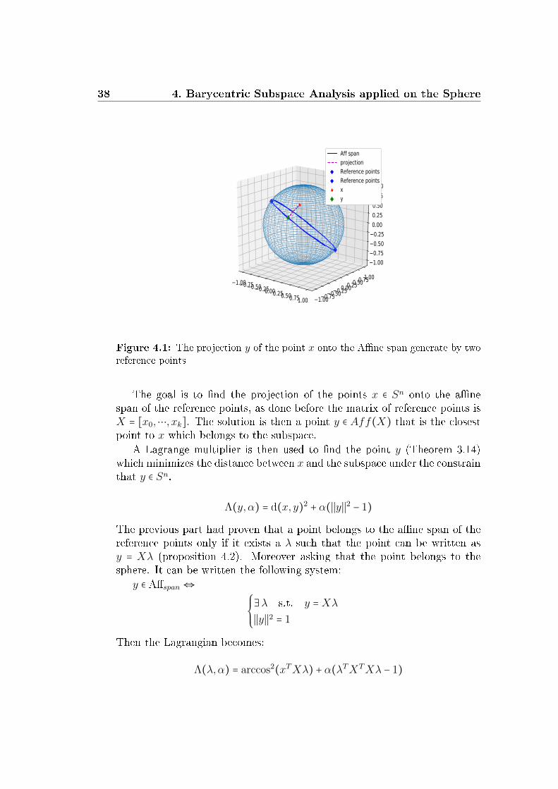
Figure 4.1: The projection y of the point x onto the Ane span generate by tworeference points
The goal is to nd the projection of the points x ∈ Sn onto the anespan of the reference points, as done before the matrix of reference points isX = [x0,⋯, xk]. The solution is then a point y ∈ Aff(X) that is the closestpoint to x which belongs to the subspace.
A Lagrange multiplier is then used to nd the point y (Theorem 3.14)which minimizes the distance between x and the subspace under the constrainthat y ∈ Sn.
Λ(y,α) = d(x, y)2 + α(∣∣y∣∣2 − 1)
The previous part had proven that a point belongs to the ane span of thereference points only if it exists a λ such that the point can be written asy = Xλ (proposition 4.2). Moreover asking that the point belongs to thesphere. It can be written the following system:
y ∈ Aspan⇔⎧⎪⎪⎨⎪⎪⎩
∃λ s.t. y =Xλ∣∣y∣∣2 = 1
Then the Lagrangian becomes:
Λ(λ,α) = arccos2(xTXλ) + α(λTXTXλ − 1)
4.2 the Sphere 39
Remark 4.4. It is important to notice before deriving that the matrix XTXmay be rank decient, if this happen the pseudo inverse of Moore-Penrosecan be used.
Deriving for α:∂Λ
∂α= 0 ⇒ λTXTXλ = 1
Deriving for λ :
∂Λ
∂λ= 0
− 2 arccos(xTXλ)√1 − (xTXλ)2
xTX + 2αλTXTX = 0
− 2θ
sin(arccos(xTy))xTX + 2αλTXTX = 0
− 2θ
sin θxTX + 2αλTXTX = 0
(αλTXTX)T = ( θ
sin(θ)xTX)
T
αXTXλ = θ
sin(θ)XTx
λ = θ
sin(θ)1
α(XTX)−1XTx
Choosing α = θsin(θ) ∣∣Xλ∣∣ = θ
sin(θ) ∣∣X(XTX)−1XTx∣∣. In conclusion the closestpoint of x in the subspace is:
y =Xλ = X(XTX)−1XTx
∣∣X(XTX)−1XTx∣∣ =x
∣∣x∣∣
4.2.2 Unexplained Variance and AUV criterion
In this section is described how to compute the unexplained variance andthe AUV criterion described in Chapter 3.2.Let's consider data points yi living on the sphere, between them are chosenthe reference ones. To compute the unexplained variance it is necessary toevaluate the projection yi of all data points onto the subspace generated bythe reference points and then the distance between the data-point and theprojection is computed, ri = dist(yi, yi). So the formula is the following:
σ2out(X) =∑
i
r2i (X) =∑
i
dist2(yi, yi(X))
40 4. Barycentric Subspace Analysis applied on the Sphere
−1.00−0.75−0.50−0.250.000.250.500.751.00 −1.00−0.75−0.50−0.250.000.250.500.751.00
−1.00−0.75−0.50−0.250.000.250.500.751.00
mean
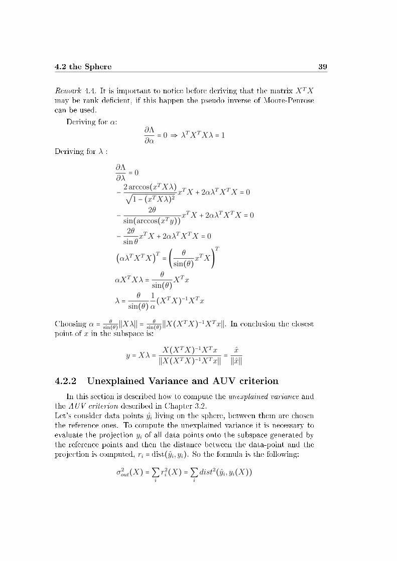
Figure 4.2: In this example there are Random points on the sphere and the meanis computed i.e. the point which minimize the sum of all the distance from theother points. This is a local maximum.
The function AUV (Accumulated Unexplained Variances described in3.2) takes the rst i-points of the reference matrix X = [x0,⋯, xi] and com-pute σout and sum it with all the previous (i−1) σout computed before addingthe i−th point. For example, the rst step is minimize the distance of thedata points with X0 = [x0], then it is done the same with the subspace gen-erated by X1 = [x0, x1] and sum up with the previous result (see gure 4.3).In general:
AUV =∑i
σouti(Xi,Data)
4.3 Testing on data 41
−1.00−0.75−0.50−0.250.000.250.500.751.00 −1.00−0.75−0.50−0.250.000.250.500.751.00
−1.00−0.75−0.50−0.250.000.250.500.751.00
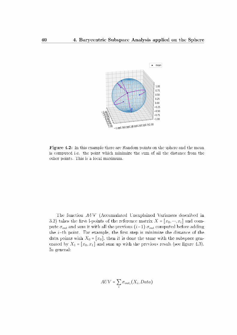
Aff spanprojectionprojectionprojectionprojectionReference pointsReference pointsxxyy
Figure 4.3: In this example we have two reference points and two data points,so the AUV function give the sum of the distance between the data points andthe rst reference point (yellow) and the distance between the data points and thesubspace of the two reference points
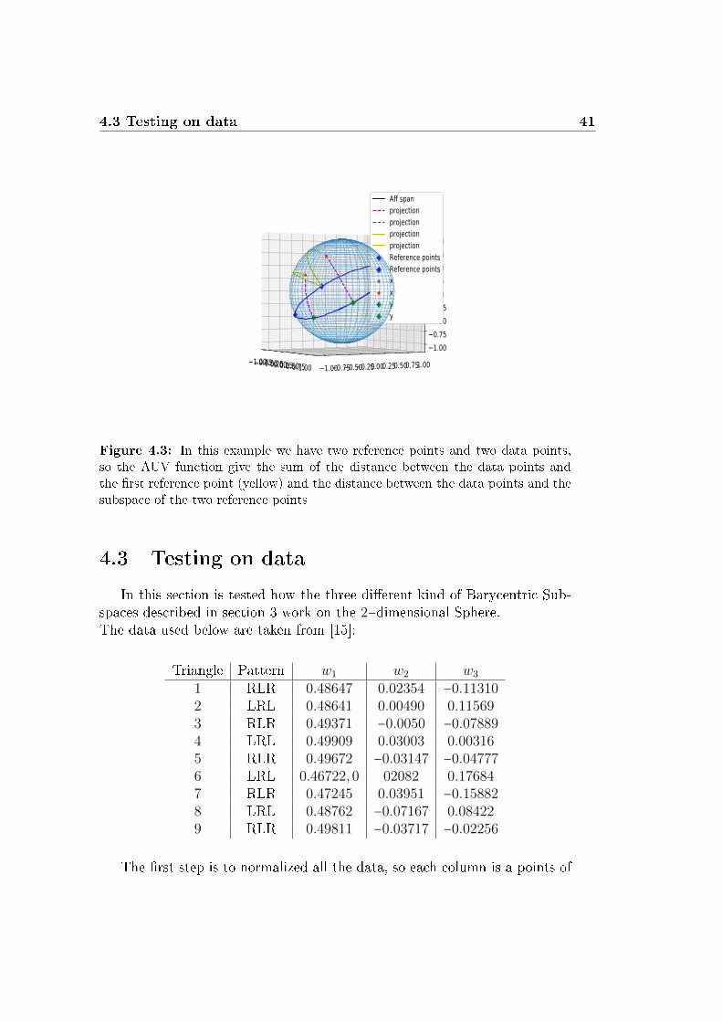
4.3 Testing on data
In this section is tested how the three dierent kind of Barycentric Sub-spaces described in section 3 work on the 2−dimensional Sphere.The data used below are taken from [15]:
Triangle Pattern w1 w2 w3
1 RLR 0.48647 0.02354 −0.113102 LRL 0.48641 0.00490 0.115693 RLR 0.49371 −0.0050 −0.078894 LRL 0.49909 0.03003 0.003165 RLR 0.49672 −0.03147 −0.047776 LRL 0.46722,0 02082 0.176847 RLR 0.47245 0.03951 −0.158828 LRL 0.48762 −0.07167 0.084229 RLR 0.49811 −0.03717 −0.02256
The rst step is to normalized all the data, so each column is a points of
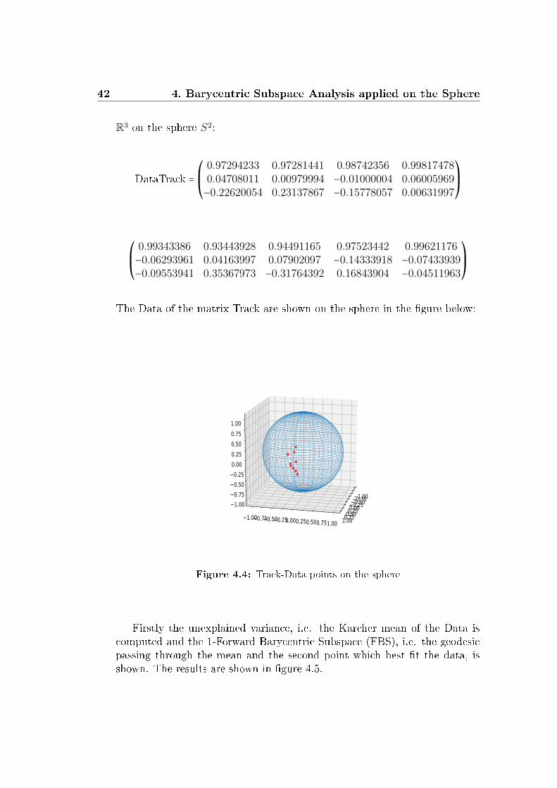
42 4. Barycentric Subspace Analysis applied on the Sphere
R3 on the sphere S2:
DataTrack =⎛⎜⎝
0.97294233 0.97281441 0.98742356 0.998174780.04708011 0.00979994 −0.01000004 0.06005969−0.22620054 0.23137867 −0.15778057 0.00631997
⎞⎟⎠
⎛⎜⎝
0.99343386 0.93443928 0.94491165 0.97523442 0.99621176−0.06293961 0.04163997 0.07902097 −0.14333918 −0.07433939−0.09553941 0.35367973 −0.31764392 0.16843904 −0.04511963
⎞⎟⎠
The Data of the matrix Track are shown on the sphere in the gure below:
−1.00−0.75−0.50−0.250.000.250.500.751.00−1.00−0.75−0.50−0.250.000.250.500.751.00
−1.00−0.75−0.50−0.250.000.250.500.751.00
Figure 4.4: Track-Data points on the sphere
Firstly the unexplained variance, i.e. the Karcher mean of the Data iscomputed and the 1-Forward Barycentric Subspace (FBS), i.e. the geodesicpassing through the mean and the second point which best t the data, isshown. The results are shown in gure 4.5.
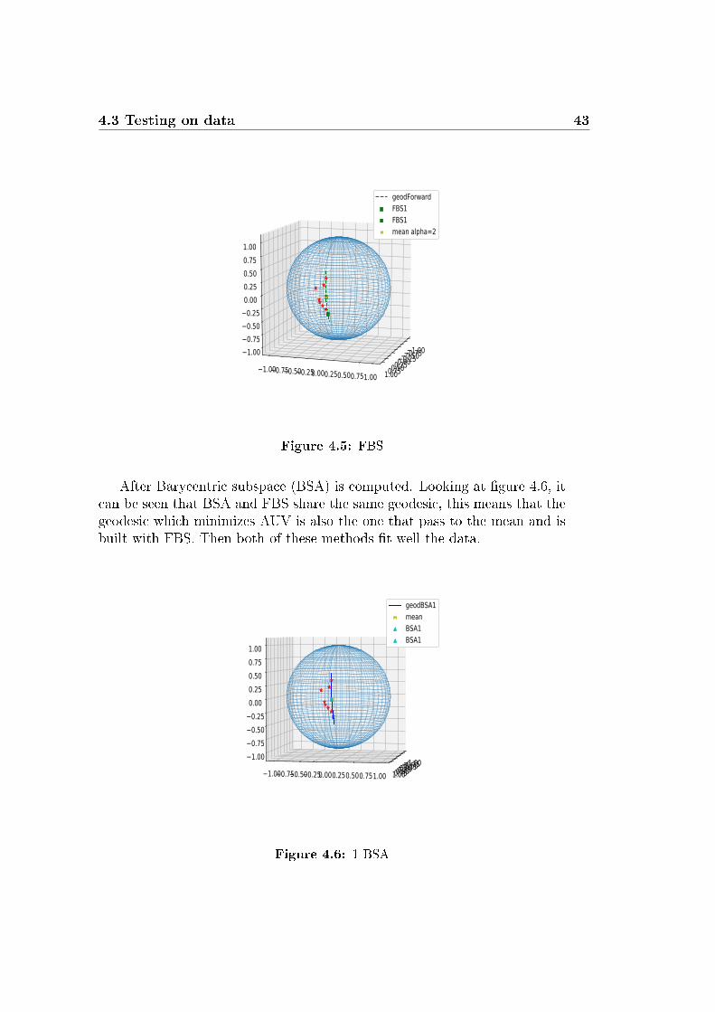
4.3 Testing on data 43
−1.00−0.75−0.50−0.250.000.250.500.751.00−1.00−0.75−0.50−0.250.000.250.500.751.00
−1.00−0.75−0.50−0.250.000.250.500.751.00
geodForwardFBS1FBS1mean alpha=2
Figure 4.5: FBS
After Barycentric subspace (BSA) is computed. Looking at gure 4.6, itcan be seen that BSA and FBS share the same geodesic, this means that thegeodesic which minimizes AUV is also the one that pass to the mean and isbuilt with FBS. Then both of these methods t well the data.
−1.00−0.75−0.50−0.250.000.250.500.751.00−1.00−0.75−0.50−0.250.000.250.500.751.00
−1.00−0.75−0.50−0.250.000.250.500.751.00
geodBSA1meanBSA1BSA1
Figure 4.6: 1-BSA

44 4. Barycentric Subspace Analysis applied on the Sphere
In gure 4.7 it is shown the resulting points using the Pure BarycentricSubspace (PBS). The resulting points are dierent from FBS and BSA. Inthe gure is also underline the three points choose with 2-PBS to show thatthe previous points chosen with 1-PBS are not xed.
−1.00−0.75−0.50−0.250.000.250.500.751.00−1.00−0.75−0.50−0.250.000.250.500.751.00
−1.00−0.75−0.50−0.250.000.250.500.751.00
geodBS2mean alpha=2PBS1PBS1PBS2PBS2PBS2
Figure 4.7: 1 and 2-Pure Barycentric subspace
−1.00−0.75−0.50−0.250.000.250.500.751.00−1.00−0.75−0.50−0.250.000.250.500.751.00
−1.00−0.75−0.50−0.250.000.250.500.751.00
geodForwardgeodBS2FBS1FBS1mean alpha=2PBS1PBS1
Figure 4.8: FBS and PBS

4.3 Testing on data 45
In conclusion the BSA and FBS gave the same results, while the PBSfound dierent reference points to build the subspace. However the data arewell tted by all the subspaces.
x axis
−1.00−0.75−0.50−0.250.000.250.500.751.00y axis
−1.00−0.75−0.50−0.250.000.250.500.751.00
z axis
−1.00−0.75−0.50−0.250.000.250.500.751.00
geodFBSgeodPBSgeodBSA
Figure 4.9: In this picture we have the Data track in red, the Mean in yellow.The geodesic for FBS are blue and are under the geodesic of BSA in light blue,while in magenta is the geodesic of PBS
4.3.1 Changing the norm
In the previews example and calculus it was used the 2−variance for com-puting the unexplained variance. Now it is interesting to study the dierenceif it is used the unexplained α−variance. As it was shown in section 3.1.1this construction is very natural with barycentric subspaces since the anespan is stable under the choice of the value α.Then the formula of α−variance:
σαout =k
∑i=0
1
αdistα(x, y)
The choice of α leads to a dierent inuence of the points. Indeed dierentnorms give dierent importance to the ouliers, data further from the otherthat can be, for example, corrupted by noise.For example, in the unit circle: the 1-norm of it in R2 is a square, the 2-normor the Eclidean norm is clearly the unit circle, while for the innity norm itis a dierent square, and for any p-norm is a superellipse.

46 4. Barycentric Subspace Analysis applied on the Sphere
So changing the norm is changing the inuences the points have on ourstudy. The test is then compute with the same data of the previous sectionchanging the value of α = 1, α = 2 and α = 0.1.The global minima of the α−variance denes the Fréchet median for the valueof α = 1, the Fréchet mean for the classical α = 2 and the barycenter of thesupport of the distribution if the value of p =∞. Indeed the dierent solutionsreach for the global minima, i.e. the rst point of FBS, are computed andlead to dierent points of the data:
0FBS2 =⎛⎜⎝
0,998174780.060059690,00631997
⎞⎟⎠
0FBS1 =⎛⎜⎝
0,99621176−0.07433939−0,04511963
⎞⎟⎠
0FBS0.1 =⎛⎜⎝
0,99343386−0.06293961−0,09553941
⎞⎟⎠
−1.00−0.75−0.50−0.250.000.250.500.751.00−1.00−0.75−0.50−0.250.000.250.500.751.00
−1.00−0.75−0.50−0.250.000.250.500.751.00
mean alpha=2mean alpha=1mean alpha=0.1
Figure 4.10: The rst point of FBS with dierent values of alpha
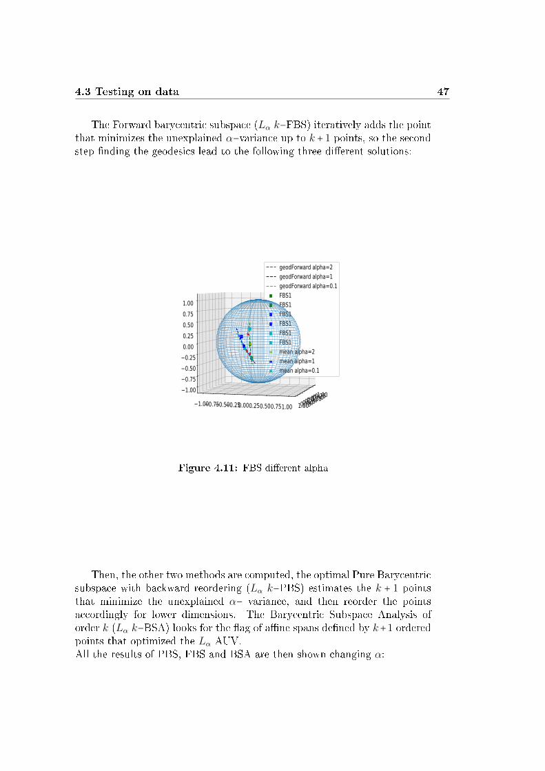
4.3 Testing on data 47
The Forward barycentric subspace (Lα k−FBS) iteratively adds the pointthat minimizes the unexplained α−variance up to k + 1 points, so the secondstep nding the geodesics lead to the following three dierent solutions:
−1.00−0.75−0.50−0.250.000.250.500.751.00−1.00−0.75−0.50−0.250.000.250.500.751.00
−1.00−0.75−0.50−0.250.000.250.500.751.00
geodForward alpha=2geodForward alpha=1geodForward alpha=0.1FBS1FBS1FBS1FBS1FBS1FBS1mean alpha=2mean alpha=1mean alpha=0.1
Figure 4.11: FBS dierent alpha
Then, the other two methods are computed, the optimal Pure Barycentricsubspace with backward reordering (Lα k−PBS) estimates the k + 1 pointsthat minimize the unexplained α− variance, and then reorder the pointsaccordingly for lower dimensions. The Barycentric Subspace Analysis oforder k (Lα k−BSA) looks for the ag of ane spans dened by k+1 orderedpoints that optimized the Lα AUV.All the results of PBS, FBS and BSA are then shown changing α:
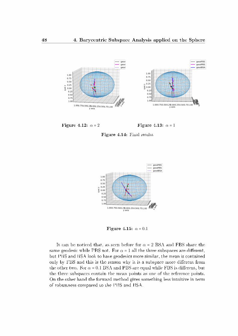
48 4. Barycentric Subspace Analysis applied on the Sphere
x axis
−1.00−0.75−0.50−0.250.000.250.500.751.00y axis
−1.00−0.75−0.50−0.250.000.250.500.751.00
z axis
−1.00−0.75−0.50−0.250.000.250.500.751.00
geodFBSgeodPBSgeodBSA
Figure 4.12: α = 2
x axis
−1.00−0.75−0.50−0.250.000.250.500.751.00y axis
−1.00−0.75−0.50−0.250.000.250.500.751.00
z axis
−1.00−0.75−0.50−0.250.000.250.500.751.00
geodFBSgeodPBSgeodBSA
Figure 4.13: α = 1
Figure 4.14: Final results
x axis
−1.00−0.75−0.50−0.250.000.250.500.751.00y axis
−1.00−0.75−0.50−0.250.000.250.500.751.00
z axis
−1.00−0.75−0.50−0.250.000.250.500.751.00
geodFBSgeodPBSgeodBSA
Figure 4.15: α = 0.1
It can be noticed that, as seen before for α = 2 BSA and FBS share thesame geodesic while PBS not. For α = 1 all the three subspaces are dierent,but PBS and BSA look to have geodesics more similar, the mean is containedonly by FBS and this is the reason why it is a subspace more dierent fromthe other two. For α = 0.1 BSA and PBS are equal while FBS is dierent, butthe three subspaces contain the mean points as one of the reference points.On the other hand the forward method gives something less intuitive in termof robustness compared to the PBS and BSA.

4.3 Testing on data 49
4.3.2 Data points random distributed
In this section it is texted the behaviour of the dierent subspaces chang-ing the norm and taking 100 random data points on the 2-dimensional Sphere.
x axis
−1.00−0.75−0.50−0.250.000.250.500.751.00y axis
−1.00−0.75−0.50−0.250.000.250.500.751.00
z axis
−1.00−0.75−0.50−0.250.000.250.500.751.00
geodForwardgeodPBS2geodBSA1meanFBS1FBS1FBS1FBS1FBS1PBS1PBS1BSA1BSA1BSA2BSA2BSA2
Figure 4.16: α = 2
x axis
−1.00−0.75−0.50−0.250.000.250.500.751.00y axis
−1.00−0.75−0.50−0.250.000.250.500.751.00
z axis
−1.00−0.75−0.50−0.250.000.250.500.751.00
geodForwardgeodPBS2geodBSA1meanFBS1FBS1FBS1FBS1FBS1PBS1PBS1BSA1BSA1BSA2BSA2BSA2
Figure 4.17: α = 1
Figure 4.18: Final results
x axis
−1.00−0.75−0.50−0.250.000.250.500.751.00y axis
−1.00−0.75−0.50−0.250.000.250.500.751.00
z axis
−1.00−0.75−0.50−0.250.000.250.500.751.00
geodForwardgeodPBS2geodBSA1meanFBS1FBS1FBS1FBS1FBS1PBS1PBS1BSA1BSA1BSA2BSA2BSA2
Figure 4.19: α = 0.1
For α = 1, FBS and BSA share the same geodesic. For α = 0.1 all thethree subspace have the same geodesic. For α = 2 all the three subspaceshave dierent geodesics.
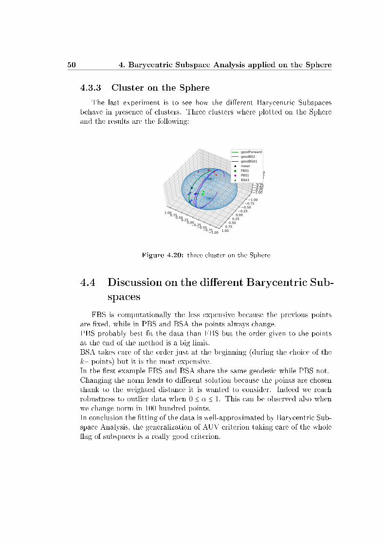
50 4. Barycentric Subspace Analysis applied on the Sphere
4.3.3 Cluster on the Sphere
The last experiment is to see how the dierent Barycentric Subspacesbehave in presence of clusters. Three clusters where plotted on the Sphereand the results are the following:
−1.00−0.75−0.50−0.250.000.250.500.751.00
−1.00−0.75
−0.50−0.25
0.000.25
0.500.75
1.00
−1.00−0.75−0.50−0.250.000.250.500.751.00
geodForwardgeodBS2geodBSA1meanFBS1PBS1BSA1
Figure 4.20: three cluster on the Sphere
4.4 Discussion on the dierent Barycentric Sub-
spaces
FBS is computationally the less expensive because the previous pointsare xed, while in PBS and BSA the points always change.PBS probably best t the data than FBS but the order given to the pointsat the end of the method is a big limit.BSA takes care of the order just at the beginning (during the choice of thek− points) but it is the most expensive.In the rst example FBS and BSA share the same geodesic while PBS not.Changing the norm leads to dierent solution because the points are chosenthank to the weighted distance it is wanted to consider. Indeed we reachrobustness to outlier data when 0 ≤ α ≤ 1. This can be observed also whenwe change norm in 100 hundred points.In conclusion the tting of the data is well-approximated by Barycentric Sub-space Analysis, the generalization of AUV criterion taking care of the wholeag of subspaces is a really good criterion.
Chapter 5
Barycentric Subspace applied on
Images
The purpose of this Chapter is to show an interesting application ofBarycentric Subspace on the problem of Image Registration. Image regis-tration is a fundamental task in medical image processing, the goal of reg-istration is to estimate the optimal transformation which maps an imageto another. This process is used to align two images. There are severaltechniques to compute the registration, one of them consists in looking fora dieomorphism which minimize the deformation between the two images,express via an energy function.
In the rst section it is provided an introduction of the general registrationmethods and it is presented the LCC Log-Demons Algorithm for referencesee [5] and [17]. The second part of the Chapter explains how use BarycentricSubspace to improve the registration with LCC Log-Demons algorithm forCardiac Motion based on the work of M.M. Rohé [13].
5.1 Image Registration
The space of images cannot be described as a standard Euclidean space,since the sum of two images is not perceived as an image:
51
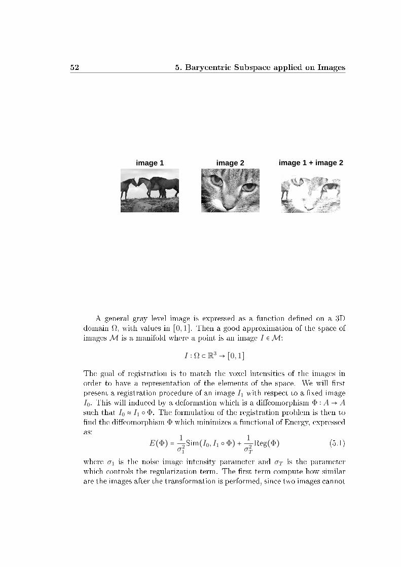
52 5. Barycentric Subspace applied on Images
image 1 image 2 image 1 + image 2
A general gray level image is expressed as a function dened on a 3Ddomain Ω, with values in [0,1]. Then a good approximation of the space ofimagesM is a manifold where a point is an image I ∈M:
I ∶ Ω ⊂ R3 → [0,1]
The goal of registration is to match the voxel intensities of the images inorder to have a representation of the elements of the space. We will rstpresent a registration procedure of an image I1 with respect to a xed imageI0. This will induced by a deformation which is a dieomorphism Φ ∶ A→ Asuch that I0 ≈ I1 Φ. The formulation of the registration problem is then tond the dieomorphism Φ which minimizes a functional of Energy, expressedas:
E(Φ) = 1
σ21
Sim(I0, I1 Φ) + 1
σ2T
Reg(Φ) (5.1)
where σ1 is the noise image intensity parameter and σT is the parameterwhich controls the regularization term. The rst term compute how similarare the images after the transformation is performed, since two images cannot
5.1 Image Registration 53
become perfectly equal and the simplest case is with L2 norm Sim(I0, I1Φ) =∥I0 − I1 Φ∥2. The second is a regularizing term of the function Φ, such thatthe transformation taken is as smaller and smoother as possible, and can bea Tikhonov regularizer.This problem is in general ill-posed problem; for this reason an additivedemons algorithm was proposed which adds a coupling term with a hiddenvariable c. Then the problem is to nd the minimum of the global energy:
E(Φ, c) = 1
σ21
Sim(I0, I1 c) +1
σ2x
dist(Φ, c)2 + 1
σ2T
Reg(Φ)
with σx is the parameter for the spatial uncertain correspondences. In generalthe last two terms of the formula can have dierent forms depending onthe problem. Note that the optimization problem give rise to two EulerLagrangian equations, obtained by dierentiating with respect to Φ and crespectively.The classic demons algorithm introduces a demons forces u obtained fromthe decomposition: c = Φ+u, which is the argument of the distance functiond. The demons forces u are an eector situated in a point of the boundaryobject. Formally u is an increment from Φ to c, so that in manifold it has tobe computed through an exponential map. In section 1.3.1 we pointed outthat we can choose as distance d(Φ, c) = ∥δv∥.
5.1.1 Log-Demons Algorithm
The Log Domain Algorithm looks for the solution of the dieomorphismΦ in the log-space. Indeed the group of Dieomorphism can be seen as a Liegroup structure, and this allows to work in its Lie algebra which is a vectorspace, so it is easier to work on compared to a manifold. We are not workingon the whole innite dimension group of dieomorphisms but in a subset ofnite dimension, but this is enough to our application. The exponential andits inverse logarithmic map, are local dieomorphisms from the Lie algebrato the Lie group and vice versa. Then the problem is not looking directlyto the dieomorphism Φ but we are looking for the one parameter subgroupgenerated by a vector eld lying in the tangent space TIdDi(Ω), i.e. theLie algebra. For a good compromise between the computational cost andthe eciency of the registration it has been proposed in [17] to work on theStationary Velocity Field (SVF). If we arbitrary x an origin in the spaceof dieomorphisms, then the one parameter subgroup Φ of a SVF v is theunique solution of:
∂Φ(x, s)∂s
= v(Φ(x, s))
54 5. Barycentric Subspace applied on Images
starting from the xed origin. Since we are working in a group (see section1.4.1), the solution is dened for s ∈ [0,1], so that we can dene exp(v) =Φ(x,1). Then we can look for v in the log-space, which is the Lie algebra.The Log-Demons functional where c = exp(w) is:
E(v,w) = 1
σ21
Sim(I0, I1 exp(w)) + 1
σ2x
dist(v,w)2 + 1
σ2T
Reg(v) (5.2)
An important property of the exponential map is the non commutative prop-erty, so that the BCH formula (1.4.2) can be used. It has been provedthat the rst two terms of the decomposition provide already a good ap-proximation if one of the terms is small, in our case: δv = BCH(−v,w) =log(exp(−v) exp(w)).This allows to minimize the functional with a two step algorithm:
1. Optimization of Similarity Given v:
E(v, δv) = 1
σ21
Sim(I0, I1 exp(v) exp(δv)) + 1
σ2x
∥δv∥2 + 1
σ2T
Reg(v)
The optimization is compute for δv, and thanks to BCH it is foundw = BCH(v, δv)
2. Optimization of Regularization Given w:
E(v,w) = 1
σ21
Sim(I0, I1exp(w))+ 1
σ2x
∥ log(exp(−v)exp(w))∥2+ 1
σ2T
Reg(v))
optimized respect to v.
5.1.2 LCC-Log Demons Functional
In [5] was proposed to replace the classical similarity measure Sim offormula 5.1 with the local correlation coecient (LCC), this is the metricused to measured the dierence between the xed image I0 and the warpedimage I1. The LCC is dened as Sim(I0, I1 Φ) = ρ(I0, I1 Φ), where
ρ(I0, I1 Φ) = ∫Ω
I0I1√I2
0I21
where I0 = Gσ ∗ I0(x) is the Gaussian smoothing applied on the image. Thecoecient varies between -1 (perfect negative correlation), 0 (no correlation)and 1 (perfect correlation). It measures how the intensities of the two imagesare correlated within a local neighborhood σ. Then the LCC similarity hasbeen used with the Log-Demons algorithm to update δv = w − v.
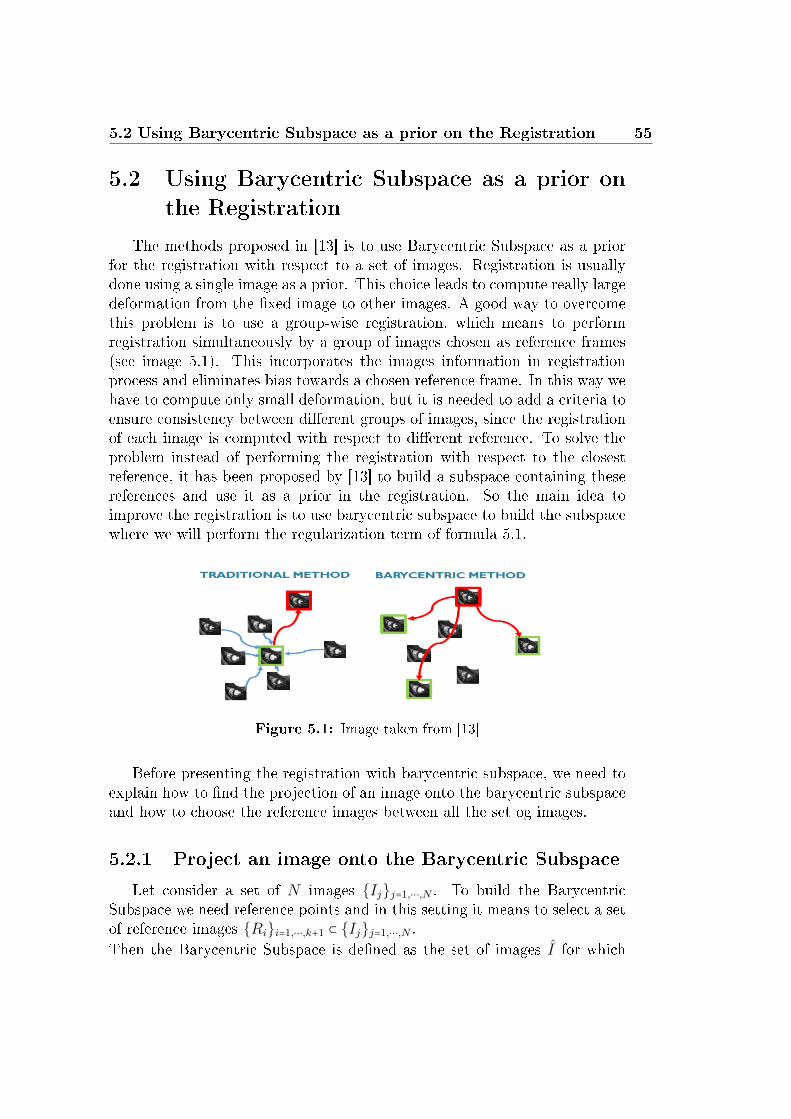
5.2 Using Barycentric Subspace as a prior on the Registration 55
5.2 Using Barycentric Subspace as a prior on
the Registration
The methods proposed in [13] is to use Barycentric Subspace as a priorfor the registration with respect to a set of images. Registration is usuallydone using a single image as a prior. This choice leads to compute really largedeformation from the xed image to other images. A good way to overcomethis problem is to use a group-wise registration, which means to performregistration simultaneously by a group of images chosen as reference frames(see image 5.1). This incorporates the images information in registrationprocess and eliminates bias towards a chosen reference frame. In this way wehave to compute only small deformation, but it is needed to add a criteria toensure consistency between dierent groups of images, since the registrationof each image is computed with respect to dierent reference. To solve theproblem instead of performing the registration with respect to the closestreference, it has been proposed by [13] to build a subspace containing thesereferences and use it as a prior in the registration. So the main idea toimprove the registration is to use barycentric subspace to build the subspacewhere we will perform the regularization term of formula 5.1.
Figure 5.1: Image taken from [13]
Before presenting the registration with barycentric subspace, we need toexplain how to nd the projection of an image onto the barycentric subspaceand how to choose the reference images between all the set og images.
5.2.1 Project an image onto the Barycentric Subspace
Let consider a set of N images Ijj=1,⋯,N . To build the BarycentricSubspace we need reference points and in this setting it means to select a setof reference images Rii=1,⋯,k+1 ⊂ Ijj=1,⋯,N .
Then the Barycentric Subspace is dened as the set of images I for which
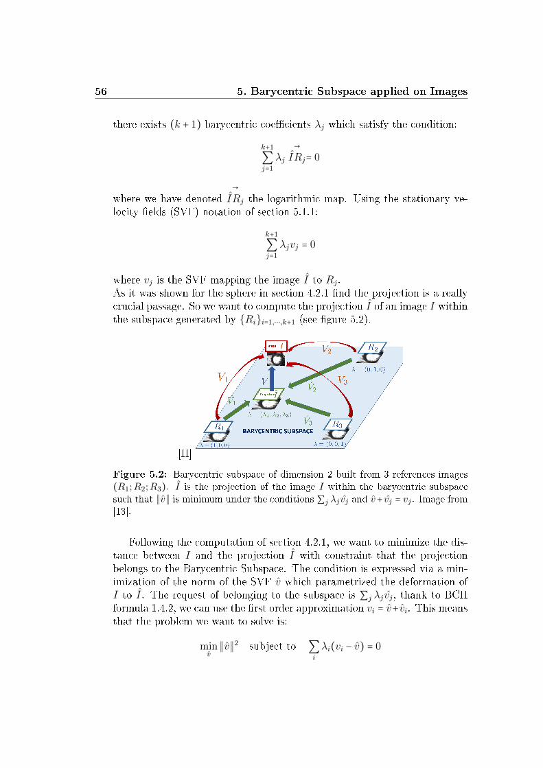
56 5. Barycentric Subspace applied on Images
there exists (k + 1) barycentric coecients λj which satisfy the condition:
k+1
∑j=1
λj
→IRj= 0
where we have denoted→IRj the logarithmic map. Using the stationary ve-
locity elds (SVF) notation of section 5.1.1:
k+1
∑j=1
λjvj = 0
where vj is the SVF mapping the image I to Rj.As it was shown for the sphere in section 4.2.1 nd the projection is a reallycrucial passage. So we want to compute the projection I of an image I withinthe subspace generated by Rii=1,⋯,k+1 (see gure 5.2).
[H]
Figure 5.2: Barycentric subspace of dimension 2 built from 3 references images(R1;R2;R3). I is the projection of the image I within the barycentric subspacesuch that ∥v∥ is minimum under the conditions ∑j λj vj and v+ vj = vj . Image from[13].
Following the computation of section 4.2.1, we want to minimize the dis-tance between I and the projection I with constraint that the projectionbelongs to the Barycentric Subspace. The condition is expressed via a min-imization of the norm of the SVF v which parametrized the deformation ofI to I. The request of belonging to the subspace is ∑j λj vj, thank to BCHformula 1.4.2, we can use the rst order approximation vi = v+vi. This meansthat the problem we want to solve is:
minv
∥v∥2 subject to ∑i
λi(vi − v) = 0
5.2 Using Barycentric Subspace as a prior on the Registration 57
requiring that ∑i λi ≠ 0. It is not restrictive to add two other constraints onthe Barycentric coecients: rst we ask ∑j λj = 1, then they are normalizedand second λi ≤ 1 such that it forces the projection to lie within a borderdened by the reference images. Then:
minv
∥v∥2 subject to v =∑i
λivi ∑j
λj = 1 λi ≤ 1
Thus the Lagrangian becomes:
Λ(λλλ,α,βββ) = ∥∑i
λivi∥2 + α(1 −∑i
λi) +βββ(1 −λλλ)
where λλλ,βββ are vectors and α a scalar. Then deriving for λj:
∂Λ(λλλ,α,βββ)∂λj
= 0
2 <∑i
λivi, vj > −α − kj = 0 ∀j
Deriving for α:
∂Λ(λλλ,α,βββ)∂α
= 0
1 −∑j
λj = 0 ∀j
From the theory of Lagrangian multiplier with inequality constraints, thelast term of the Lagrangian adds to the system two equations: βj ≥ 0 andβj(1−λj) = 0 for all j. So the solution can be found by solving the followingsystem:
⎧⎪⎪⎪⎪⎪⎪⎪⎨⎪⎪⎪⎪⎪⎪⎪⎩
< ∑i λivi, vj >=α+kj
2 ∀j∑j λj = 1 ∀jβj(1 − λj) = 0 ∀jβj ≥ 0 ∀j
The analysis is divided in two cases if βj = 0 or (1 − λj) = 0.If all βj are zero, then the inequality constraint is not lled and so we have tosolve < ∑i λivi, vj >= α
2 for all j. Denoting S the matrix of the scalar productSij =< vi, vj >:
Sλλλ = α111
Adding the condition: ∑i λi = 1 for all j, the optimal barycentric coecientsλλλ∗:
λλλ∗ = S−1111
∑i(S−1111)i
58 5. Barycentric Subspace applied on Images
The second case is if some βj are dierent from zero, then λi = 1 for theseindices. Then we have to solve a lower dimensional problem removing theconstrains already satised.In conclusion, we have found the barycentric coordinates which allow us tond the SVF v just computing the weighted sum: v = ∑i λ
∗i vi. Then the
projected image I is given:
I = I exp(v)
5.2.2 Choice of the reference images for cardiac motion
It is necessary to dene a criterion to choose the reference images Rii=1,⋯,k+1
within the set of images Ijj=1,⋯,N . The method proposed in [13] is to usean optimization approach. It consists on trying all the possible combinationof k + 1 references and choose the set of them that minimize the followingfunctional:
(R1,⋯,Rk+1) = arg minE(R1,⋯,Rk+1) = arg min∑j
∥vj∥2 (5.3)
where vj is the projection of the image Ij to the barycentric subspace denedby (R1,⋯,Rk+1).
5.2.3 Barycentric Log-Demons Algorithm
Lastly we are going to explain the idea to improve the registration thanksto Barycentric Subspace. This is done using Barycentric Subspace as a prior.The goal is to nd the registration of an image I ∈ Ijj=1,⋯,N with respectto all the reference images Rj chosen between the set of images Ijj=1,⋯,Nusing 5.3. The methodology of barycentric subspace is used in combinationwith LCC Log-Domain Dieomorphic Demons algorithm described in section5.1.2.The rst step is to initialize the algorithm with the standard registration ofthe image I with each references to get the SVF v0
j . Using the projectiononto the subspace explain in section 5.2.1 we can nd the rst approximationof the SVF v0 which encodes the distance between I and the subspace. Sincewe have v0
j and v0, we can nd with BCH formula the SVF v0
j which encodes
the distance between the reference Rj and the projected image I. This allows
us to compute the warped references R0i = Ri exp v0.
Then the algorithm proceeds iterating the process, but using Ri in place ofRi. Introducing these warped references will allow to look for an incrementin the deformation spaces, instead of the full deformation. In the iteration

5.2 Using Barycentric Subspace as a prior on the Registration 59
we project the update demons forces (i.e. u) on the barycentric velocity untilconvergence, when Rj
i = Ri exp(vji ) is under the xed threshold.At the end of the iteration we look for the SVF v by mapping each warped
reference Rij to the current image and compose this SVF with the barycentric
velocity to get an estimation of the full deformation: vji = vji + v. In this way
we have found the deformation vji mapping symmetrically each reference tothe image.
5.2.4 Representation of Cardiac Motion using Baryn-
centric Subspace
The method described in section 5.2.3 has been introduced in [13] to studycardiac motion. In the context of cardiac motion analysis, a cardiac cycle isdescribed as a sequence of gray level images. A rst step of the analysis isto nd correspondences - the registration step - between each of the frame ofthe sequence. It allows to track the motion of the myocardium and computedeformation elds representing the motion during a cycle.In a sequence of frames of cardiac motion, the regularization usually is doneusing one image (usually end diastole (ED)) as a prior. This choice leads tocompute really large deformation from the ED to other images (for exampleto end systole (ES) image, see gure 5.3). Then the use of the methodologydescribed is proposed.
Figure 5.3: This image taken from [13] shows the dierence of the classical regis-tration approach for cardiac motion compared to the group-wise approach proposedwith Barycentric Subspace.
The evaluation of the method is performed in [13] using one synthetic timeserie of T = 30 cardiac image frames. The use of a synthetic sequence has theimportant advantage to provide a dense point correspondence eld followingthe motion of the myocardium during the cardiac cycle which can be usedto evaluate the accuracy of tracking. In gure 5.4 it is shown a comparisonthe barycentric approach with the standard approach where the registrationbetween one of the reference and the current frame is done directly.The barycentric method leads to a substantial reduction of the error (about
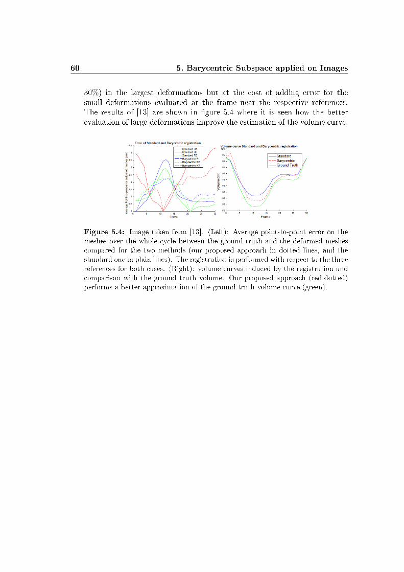
60 5. Barycentric Subspace applied on Images
30%) in the largest deformations but at the cost of adding error for thesmall deformations evaluated at the frame near the respective references.The results of [13] are shown in gure 5.4 where it is seen how the betterevaluation of large deformations improve the estimation of the volume curve.
Figure 5.4: Image taken from [13]. (Left): Average point-to-point error on themeshes over the whole cycle between the ground-truth and the deformed meshescompared for the two methods (our proposed approach in dotted lines, and thestandard one in plain lines). The registration is performed with respect to the threereferences for both cases. (Right): volume curves induced by the registration andcomparison with the ground truth volume. Our proposed approach (red-dotted)performs a better approximation of the ground truth volume curve (green).
Chapter 6
Conclusion
In this thesis it was investigated the Barycentric Subspace Analysis. Wepresented dierent kind of barycentric subspaces depending on the choice ofdenition of mean, the three denitions lead to nested subspaces. We showedthat the ane subspace in a Euclidean space can be generalized to manifoldsthank to the denition of ane spans as the metric completion of Exponen-tial Barycentric Subspace. This subspace is complete and this ensure thatalways exists a closest point on the subspace which is really important as weshowed in the two example. We also saw that the denition of ane span isstable under the choice of dierent norm. Noticing that the ane subspacescan be easily nested as in the Euclidean case, it was presented the general-ization of PCA: Barycentric Subspace Analysis.Then we presented a deep studies on the Sphere showing that in this manifoldthe Barycentric Subspace are the great circle passing through the referencepoints. We showed how the three dierent methods: forward barycentricsubspace, pure barycentric subspace and barycentric subspace analysis workon the Sphere. All this methods well-t the data living on the Sphere, butthe best tting is the barycentric subspace analysis since it takes care of thewhole ag of subspace using the AUV criterion.Then we presented how the use of Barycentric Subspace can improve the reg-istration in cardiac motion. It relies on building subspaces as the referencefor registration instead of choosing a single image. So we presented how tochoose the reference images, how to project an image inside the barycentricsubspace and we concluded presenting the Barycentric Log-Demons Algo-rithm which performs and improves the registration step.
61

62 6. Conclusion
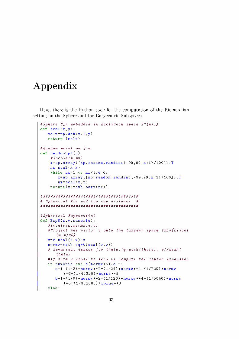
Appendix
Here, there is the Python code for the computation of the Riemanniansetting on the Sphere and the Barycentric Subspaces.
#Sphere S_n embedded in Euclidean space R^n+1
def scal(x,y):
molt=np.dot(x.T,y)
return (molt)
#Random point on S_n
def RandomSph(n):
#locals(x,xn)
x=np.array ([np.random.randint (-99,99,n+1) /100]).T
nx=scal(x,x)
while nx >1 or nx <1.e-6:
x=np.array ([np.random.randint (-99,99,n+1) /100]).T
nx=scal(x,x)
return(x/math.sqrt(nx))
#######################################
# Spherical Exp and Log map distance #
#######################################
#Spherical Exponential
def ExpS(x,v,numeric):
#locals(w,normw ,a,b)
#Project the vector v onto the tangent space TxS=w|scal
(w,x)=0
w=v-scal(x,v)*x
normw=math.sqrt(scal(w,w))
# Numerical issues for theta .(y-cosh(theta). x)/sinh(
theta)
#if norm w close to zero we compute the Taylor expansion
if numeric and N(normw) <1.e-6:
a=1 -(1/2)*normw **2+(1/24)*normw **4 -(1/720)*normw
**6+(1/40320)*normw **8
b=1 -(1/6)*normw **2+(1/120)*normw **4 -(1/5040)*normw
**6+(1/362880)*normw **8
else:
63
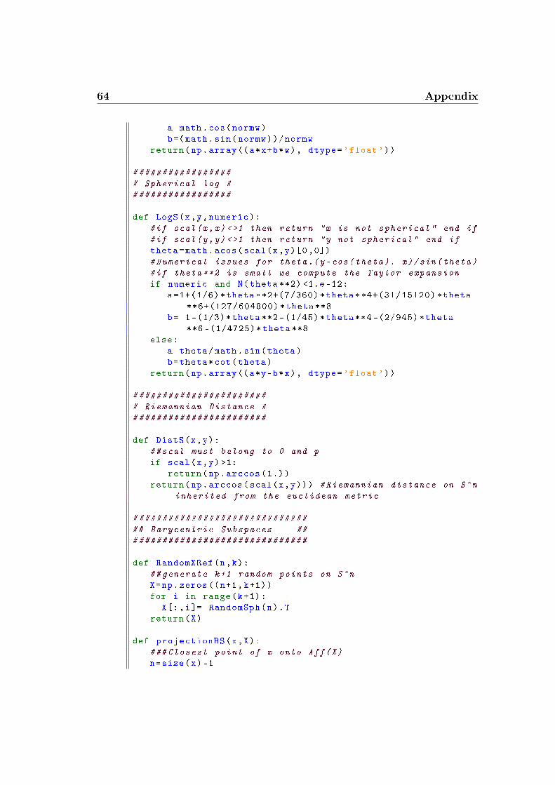
64 Appendix
a=math.cos(normw)
b=(math.sin(normw))/normw
return(np.array((a*x+b*w), dtype='float'))
#################
# Spherical log #
#################
def LogS(x,y,numeric):
#if scal(x,x) <>1 then return "x is not spherical" end if
#if scal(y,y) <>1 then return "y not spherical" end if
theta=math.acos(scal(x,y)[0,0])
#Numerical issues for theta .(y-cos(theta). x)/sin(theta)
#if theta **2 is small we compute the Taylor expansion
if numeric and N(theta **2) <1.e-12:
a=1+(1/6)*theta **2+(7/360)*theta **4+(31/15120)*theta
**6+(127/604800)*theta **8
b= 1 -(1/3)*theta **2 -(1/45)*theta **4 -(2/945)*theta
**6 -(1/4725)*theta **8
else:
a=theta/math.sin(theta)
b=theta*cot(theta)
return(np.array((a*y-b*x), dtype='float'))
#######################
# Riemannian Distance #
#######################
def DistS(x,y):
##scal must belong to 0 and p
if scal(x,y) >1:
return(np.arccos (1.))
return(np.arccos(scal(x,y))) #Riemannian distance on S^n
inherited from the euclidean metric
##############################
## Barycentric Subspaces ##
##############################
def RandomXRef(n,k):
##generate k+1 random points on S^n
X=np.zeros ((n+1,k+1))
for i in range(k+1):
X[:,i]= RandomSph(n).T
return(X)
def projectionBS(x,X):
### Closest point of x onto Aff(X)
n=size(x) -1
65
Omega=np.dot(X.T,X)
Omega=np.linalg.pinv(Omega)
#Unconstrained projection on Aff(X)
z=np.dot(np.dot(np.dot(X,Omega),X.T),x)
return(z/math.sqrt(scal(x,z)))
def CoordOnBS(x,X):
### Coordinates on Aff(X)
Omega=np.dot(X.T,X)
# Unconstrained projection on Aff(X)
w=np.dot(np.dot(np.linalg.pinv(Omega),X.T),x)
return(w/math.sqrt(scal(x,np.dot(X,w))))
###############################
## alpha change the norm ##
###############################
def sigma_out(X,Data ,alpha):
##sigma_out(X)=Sum(Residue **2(X))=Sum(dist **2(x,y))
sig=0.
for i in range(size(Data [0 ,:])):
x=np.array ([Data[:,i]]).T
y=projectionBS(x,X)
res=(abs(DistS(x,y)))**alpha/alpha
sig=sig+res
return(sig/(size(Data [0 ,:])))
def AUC(X,Data ,alpha):
##AUC=Sum(sigma_out(Xi ,Data))
AUCtmp =0
for i in range(1,size(X[0,:])+1):
#select firts i points
Xi=X[:,0:i]#in maple Xi := X[1.. -1 ,1..i]; I take the
first i points of X
sigi=sigma_out(Xi,Data ,alpha)
AUCtmp=AUCtmp+sigi
return(AUCtmp)
###############################
## Best point approx of data ##
###############################
def DataMean(Data ,alpha):
### initialize with first point
x=np.array ([Data [: ,0]]).T
sigmin=sigma_out(x,Data ,alpha)
for i in range(1,size(Data [0 ,:])):
sig=sigma_out(np.array ([Data[:,i]]).T,Data ,alpha)
if N(sig <sigmin):

66 Appendix
sigmin=sig
x=np.array ([Data[:,i]]).T
return(x,N(sigmin))
#########
## FBS ##
#########
##Compute next mode
def ForwardBS(Xin ,Data ,alpha):
##Compute the Forward Barycentric Subspace: minimizing
sigma_out
X=Xin
sigmin=sigma_out(X,Data ,alpha)
for i in range(size(Data [0 ,:])):
Xtest=np.concatenate ((Xin ,np.array ([Data[:,i]]).T),
axis =1)
sig=sigma_out(Xtest ,Data ,alpha)
if N(sig <sigmin):
sigmin=sig
X=Xtest
return(X,N(sigmin))
#########
## PBS ##
#########
def SwapCol(X,i,j):
##Function that swap the column i and j of a matrix X
col=np.copy(X[:,i])
X[:,i]=X[:,j]
X[:,j]=col
return(X)
def Compute_PBS1(Data ,alpha):
## 1-Pure Barycentric subspace = optimal geodesic
X=Data [: ,0:2]#Take column 0 and column 1
sigmin=sigma_out(X, Data ,alpha)
for i in range(size(Data [0 ,:])):
for j in range(i+1,size(Data [0 ,:])):
Xtest=np.concatenate ((np.array([Data[:,i]]).T,np.
array ([Data[:,j]]).T),axis =1)
sig=sigma_out(Xtest ,Data ,alpha)
if N(sig <sigmin):
sigmin=sig
X=Xtest
## Reorder the 2 points
if N(sigma_out(np.array ([X[: ,0]]).T,Data ,alpha))>N(
sigma_out(np.array([X[: ,1]]).T,Data ,alpha)):
67
SwapCol(X,0,1)
return(X,N(sigmin))
def Compute_PBS2(Data ,alpha):
## 2-Pure Barycentric subspace
X=Data [: ,0:3]
sigmin=sigma_out(X, Data ,alpha)
for i in range(size(Data [0 ,:])):
for j in range(i+1,size(Data [0 ,:])):
for k in range(j+1,size(Data [0 ,:])):
Xtest=np.concatenate ((np.array([Data[:,i]]).T,
np.array([Data[:,j]]).T,np.array ([Data[:,k
]]).T),axis =1)
sig=sigma_out(Xtest ,Data ,alpha)
if N(sig <sigmin):
sigmin=sig
X=Xtest
# Reorder the 3 points
# find minimum
sigmin=N(sigma_out(np.array ([X[: ,0]]).T,Data ,alpha))
imin=0
for i in range (1,3):
sig=N(sigma_out(np.array ([X[:,i]]).T,Data ,alpha))
if sig <sigmin:
imin=i
sigmin=sig
X=SwapCol(X,0,imin)#0 or 1??
Xtest=np.concatenate ((np.array([X[: ,0]]).T,np.array([X
[: ,2]]).T),axis =1)
if N(sigma_out(X[:,0:2],Data ,alpha))>N(sigma_out(Xtest ,
Data ,alpha)):
X=SwapCol(X,1,2)## X := < X[1.. -1 ,1] | X[1.. -1 ,3]
| X[1.. -1,2]
return(X,N(sigma_out(X,Data ,alpha)))
def Compute_PBS3(Data ,alpha):
## 3-Pure Barycentric subspace
X=Data [: ,0:4]
sigmin=sigma_out(X,Data ,alpha)
for i in range(size(Data [0 ,:])):
for j in range(i+1,size(Data [0 ,:])):
for k in range(j+1,size(Data [0 ,:])):
for l in range(k+1,size(Data [0 ,:])):
Xtest=np.concatenate ((np.array([Data[:,i]]).
T,np.array([Data[:,j]]).T,np.array([Data
[:,k]]).T,np.array ([Data[:,l]]).T),axis
=1)
sig=sigma_out(Xtest ,Data ,alpha)
if N(sig <sigmin):
68 Appendix
sigmin=sig
X=Xtest
## Reorder the 4 points
## find minimum
sigmin=sigma_out(np.array ([X[: ,0]]).T,Data ,alpha)
imin=0
for i in range (1,4):
sig=N(sigma_out(np.array ([X[:,i]]).T,Data ,alpha))
if sig <sigmin:
imin=i
sigmin=sig
#exchange point 1 with imin
SwapCol(X,0,imin)
#Now repeat for the minimum pair
imin=1
sigmin=N(sigma_out(X[:,0:2],Data ,alpha))
for i in range (2,4):
sig=N(sigma_out(np.concatenate ((np.array([X[: ,0]]).T,
np.array([X[:,i]]).T),axis =1),Data ,alpha))
if sig <sigmin:
imin=i
sigmin=sig
#Exchange X[1] with X[imin]
if imin >2:
SwapCol(X,1,imin)
#last level
if N(sigma_out(np.concatenate ((np.array(X[: ,0:2]),np.
array ([X[: ,3]]).T),axis =1),Data ,alpha))<N(sigma_out(
np.array(X[: ,0:3]),Data ,alpha)):
SwapCol(X,2,3)
return(X,N(sigma_out(X,Data ,alpha)))
#########
## BSA ##
#########
def Compute_BSA1(Data ,alpha):
## 1-BSA # with less calculus: time divided by 6
## minimizing AUC
X=Data [: ,0:2]
aucmin=AUC(X,Data ,alpha)
for i in range(size(Data [0 ,:])):
X1=np.array([Data[:,i]]).T
sig1=sigma_out(X1,Data ,alpha)
if sig1 <aucmin:# otherwise sig1 + something cannot be
smaller than aucmin
for j in range(size(Data [0 ,:])):
Xtest=np.concatenate ((X1 ,np.array ([Data[:,j]]).
T),axis =1)
69
auc=sig1+sigma_out(Xtest ,Data ,alpha)
if N(auc <aucmin):
aucmin=auc
X=Xtest
return(X,N(aucmin))
def Compute_BSA2(Data ,alpha):
## 2-BSA # time divided by 20! (4.3 instead of 85 on
Tracks)
X=Data [: ,0:3]
aucmin=AUC(X,Data ,alpha)
for i in range(size(Data [0 ,:])):
X1=np.array([Data[:,i]]).T
auc1=sigma_out(X1,Data ,alpha)
if auc1 <aucmin:# otherwise auc1 + something cannot be
smaller than aucmin
for j in range(size(Data [0 ,:])):
X2=np.concatenate ((X1,np.array ([Data[:,j]]).T),
axis =1)
auc2=auc1+sigma_out(X2,Data ,alpha)
if auc2 <aucmin:# otherwise auc2 + something
cannot be smaller than aucmin
for k in range(size(Data [0 ,:])):
X3=np.concatenate ((X2,np.array ([Data[:,k
]]).T),axis =1)
auc3=auc2+sigma_out(X3,Data ,alpha)
if N(auc3 <aucmin):
aucmin=auc3
X=X3
return(X,N(aucmin))
def Compute_BSA3(Data ,alpha):
## 3-BSA
X=Data [: ,0:4]
aucmin=AUC(X,Data ,alpha)
for i in range(size(Data [0 ,:])):
#print('Iteration /n',i)
X1=np.array([Data[:,i]]).T
auc1=sigma_out(X1,Data ,alpha)
if auc1 <aucmin:# otherwise auc1 + something cannot be
smaller than aucmin
for j in range(size(Data [0 ,:])):
X2=np.concatenate ((X1,np.array ([Data[:,j]]).T),
axis =1)
auc2=auc1+sigma_out(X2,Data ,alpha)
if auc2 <aucmin:## otherwise auc2 + something
cannot be smaller than aucmin
for k in range(size(Data [0 ,:])):
70 Appendix
X3=np.concatenate ((X2,np.array ([Data[:,k
]]).T),axis =1)
auc3=auc2+sigma_out(X3,Data ,alpha)
if auc3 <aucmin:
for l in range(size(Data [0 ,:])):
X4=np.concatenate ((X3,np.array ([
Data[:,l]]).T),axis =1)
auc4=auc3+sigma_out(X4,Data ,alpha)
if N(auc4 <aucmin):
aucmin=auc4
X=X4
return(X,N(aucmin))

Bibliography
[1] Bauer, M., Bruveris, M., Michor, P.W. Uniqueness of the Fisher-Raometric on the space of smooth densities.
[2] Joshi, S., Srivastava, A., Jermyn, I.H. (2007) Riemannian analysis ofprobability density functions with applications in vision., in 2007 IEEEConference on Computer Vision and Pattern Recognition ; proceedings.Piscataway, NJ: IEEE, pp. 1664-1671.
[3] Joshi, S., Davis, B., Jomier, M., Gerig, G., Unbiased dieomorphic atlasconstruction for computational anatomy, NeuroImage, Elsevier, 2004.
[4] Jost, J. Riemannian Geometry and Geometric analysis, Springer, 2008,fth edition.
[5] Lorenzi, M., Ayache, N., Frisoni, G., Pennec, X. LCC-Demons: a robustand accurate symmetric dieomorphic registration algorithm. NeuroIm-age, Elsevier, 2013, 81 (1), pp. 470-483.
[6] Lorenzi, M., Pennec, X., Geodesics, Parallel Transport, One-parameterSubgroups for Dieomorphic Image Registration International Journal ofComputer Vision, Springer Verlag, 2013, International Journal of Com-puter Vision, 105(2), pp. 111-127.
[7] Pennec, X. Barycentric Subspace Analysis on Manifold, Submitted tothe Annals of Statistics, imsart-aos ver. 2017 .
[8] Pennec, X., Arsigny, V. Exponential Barycenters of the Canonical Car-tan Connection and Invariant Means on Lie Groups. Frederic Bar-baresco and Amit Mishra and Frank Nielsen. Matrix Information Ge-ometry, Springer, pp. 123-168, 2012, 978-3-642-30231.
[9] Pennec, X. From Riemannian Geometry to Computational Anatomy,Asclepios project-team, INRIA Sophia-Antipolis Mediterranee, 2011.
71

72 BIBLIOGRAPHY
[10] Pennec, X. Intrinsic Statistics on Riemannian Manifolds: Basic Toolsfor Geometric Measurements. Journal of Mathematical Imaging and Vi-sion, Springer Verlag, 2006, 25(1), pp.127-154.
[11] Pennec, X. Sample-limited Lp Barycentric Subspace Analysis on Con-stant Curvature Spaces Nov 2017, Paris, France. Springer InternationalPublishing, Lecture Notes in Computer Science (LNCS), pp.20-28, 2017,Geometric Science of Information.
[12] Rohé, M.M., Sermesant, M., Pennec, X. Barycentric Subspace Analy-sis: a new Symmetric Group-wise Paradigm for Cardiac Motion Track-ing. MICCAI 2016-the 19th International Conference on Medical Im-age Computing and Cmputer Assisted Intervention, Oct 2016, Athens,Greece 9902 (448-456), pp. 300-307,2016 MICCAI 2016, Lecture Notesin Computer Science.
[13] Rohé, M.M, Sermesant, M., Pennec,X Low-Dimensional Representationof Cardiac Motion Using Barycentric Subspaces: a New Group-WiseParadigm for Estimation, Analysis, and Reconstruction.
[14] Rohé, M.M. Reduced representation of segmentation and tracking in car-diac images for group-wise longitudinal analysis PhD Thesis, UniversitéCôte d'Azur, July 2017.
[15] Small, Christopher G. The Statistical Theory of Shape, Springer seriesin statistics, 1996.
[16] Tu, L.W. An introduction to Manifolds, Springer, 2011, second edition.
[17] Vercauteren T., Pennec X., Perchant A., Ayache N.,2008 Symmetriclog-domain dieomorphic registration: A demons-based approach Proc.Medical Image Computing and Computer Assisted Intervention (MIC-CAI'08), Part I, Springer, New York, USA, pp. 754-761.
[18] Warner F. Fundamentation of dierentiable maanifold, University ofPennsylvania, Scott Foresman and Company.
[19] Wilkins, D. R. A Course in Riemannian Geometry, 2005.