generalized barycentric coordinates in computer...

Kai Hormann, N. Sukumar

Generalized BarycentricCoordinates inComputer Graphics andComputational Mechanics

Contents

Chapter 1 � Multi-Sided Patches via Barycentric Coordinates 1

Scott Schaefer

1.1 INTRODUCTION 11.1.1 Bezier Form of Curves 21.1.2 Evaluation 31.1.3 Degree Elevation 4

1.2 MULTISIDED BEZIER PATCHES IN HIGHER DIMENSIONS 41.2.1 Indexing For S-Patches 51.2.2 Evaluation 71.2.3 Degree Elevation 8

1.3 APPLICATIONS 91.3.1 Surface patches 91.3.2 Spatial Deformation 10

iii

C H A P T E R 1

S-PatchesScott SchaeferTexas A&M University

CONTENTS

1.1 Introduction . . . . . . . . . . . . . . . . . . . . . . . . . . . . . . . . . . . . . . . . . . . . . . . . . 11.1.1 Bezier Form of Curves . . . . . . . . . . . . . . . . . . . . . . . . . . . . . . 21.1.2 Evaluation . . . . . . . . . . . . . . . . . . . . . . . . . . . . . . . . . . . . . . . . . . . 31.1.3 Degree Elevation . . . . . . . . . . . . . . . . . . . . . . . . . . . . . . . . . . . . 4

1.2 Multisided Bezier Patches in Higher Dimensions . . . . . . . . . . . 41.2.1 Indexing For S-Patches . . . . . . . . . . . . . . . . . . . . . . . . . . . . . 51.2.2 Evaluation . . . . . . . . . . . . . . . . . . . . . . . . . . . . . . . . . . . . . . . . . . . 71.2.3 Degree Elevation . . . . . . . . . . . . . . . . . . . . . . . . . . . . . . . . . . . . 8

1.3 Applications . . . . . . . . . . . . . . . . . . . . . . . . . . . . . . . . . . . . . . . . . . . . . . . . . 91.3.1 Surface patches . . . . . . . . . . . . . . . . . . . . . . . . . . . . . . . . . . . . . . 91.3.2 Spatial Deformation . . . . . . . . . . . . . . . . . . . . . . . . . . . . . . . . . 10

CHAPTER ?? introduced several constructions of barycentric coordinatesas well as their properties. In this chapter, we explore the deep connection

between barycentric coordinates and higher order parametric representations ofcurves, surfaces, volumes in arbitrary dimension. In the case of curves, these curvesare known as Bezier curves, which are used in applications from font representa-tions to controlling animations. The extension to convex surface patches, calledS-Patches [7], is more recent. As originally proposed, S-Patches were parametric,multi-sided surface patches restricted to convex domains. However, these restric-tions were more of a function of the limited set of generalized barycentric coor-dinates, namely Wachspress coordinates, available at that time. Today we havegeneralized barycentric coordinate functions that do not require convexity and ex-tend to arbitrary dimension. Hence, we will investigate S-Patches within their fullgenerality afforded by modern barycentric coordinates with generalized domainsand in arbitrary dimension.

1.1 INTRODUCTION

1

2 � Generalized Barycentric Coordinates inComputer Graphics and Computational Mechanics

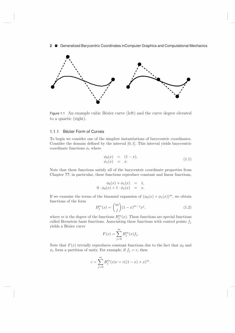
Figure 1.1 An example cubic Bezier curve (left) and the curve degree elevatedto a quartic (right).

1.1.1 Bezier Form of Curves

To begin we consider one of the simplest instantiations of barycentric coordinates.Consider the domain defined by the interval [0, 1]. This interval yields barycentriccoordinate functions ϕi where

ϕ0(x) = (1 − x),ϕ1(x) = x.

(1.1)

Note that these functions satisfy all of the barycentric coordinate properties fromChapter ??; in particular, these functions reproduce constant and linear functions,

ϕ0(x) + ϕ1(x) = 1,0 · ϕ0(x) + 1 · ϕ1(x) = x.

If we examine the terms of the binomial expansion of (ϕ0(x) + ϕ1(x))m, we obtainfunctions of the form

Bmj (x) =

(m

j

)(1 − x)m−jxj , (1.2)

where m is the degree of the functions Bmj (x). These functions are special functions

called Bernstein basis functions. Associating these functions with control points fj

yields a Bezier curve

F (x) =m∑

j=0Bm

j (x)fj .

Note that F (x) trivially reproduces constant functions due to the fact that ϕ0 andϕ1 form a partition of unity. For example, if fj = c, then

c =m∑

j=0Bm

j (x)c = c((1 − x) + x)m.

Multi-Sided Patches via Barycentric Coordinates � 3

0p 1p

10 pbpa +

a b

Figure 1.2 An example pyramid diagram. The values at the base are multipliedby the constants on the arrows and summed to produce the result at the apexof the pyramid.

In addition, F (x) can also reproduce all polynomial functions up to degree m. Thislast property follows directly from the linear reproduction property of barycentriccoordinates. In particular, to reproduce a function xk where k ≤ m there existscoefficients fj such that

F (x) = (ϕ0(x) + ϕ1(x))m−k(0 · ϕ0(x) + 1 · ϕ1(x))k = 1m−kxk = xk

where the coefficients fj are given by collecting the coefficients of Bmj (x) in the

polynomial expansion above. For example, to reproduce the function x, the coeffi-cients are given by fj = j

m . Such properties also follow directly from the theory ofblossoming/polar forms [8], which is beyond the scope of this chapter.

In addition, the barycentric coordinate functions ϕi also impart a number ofuseful geometric properties on the resulting Bezier curves. For example, Beziercurves interpolate their end points due to the Lagrange property of barycentriccoordinates. Bezier curves also fall within the convex hull of their control points overthe interval [0, 1] since 0 ≤ ϕi(x) ≤ 1 for all x ∈ [0, 1]. The curves are also affinelyinvariant; that is, transforming each control point by an affine transformation Ttransforms the Bezier curve by T . Figure 1.1 shows an example of a Bezier curvewhere the fj are points in R2.

1.1.2 Evaluation

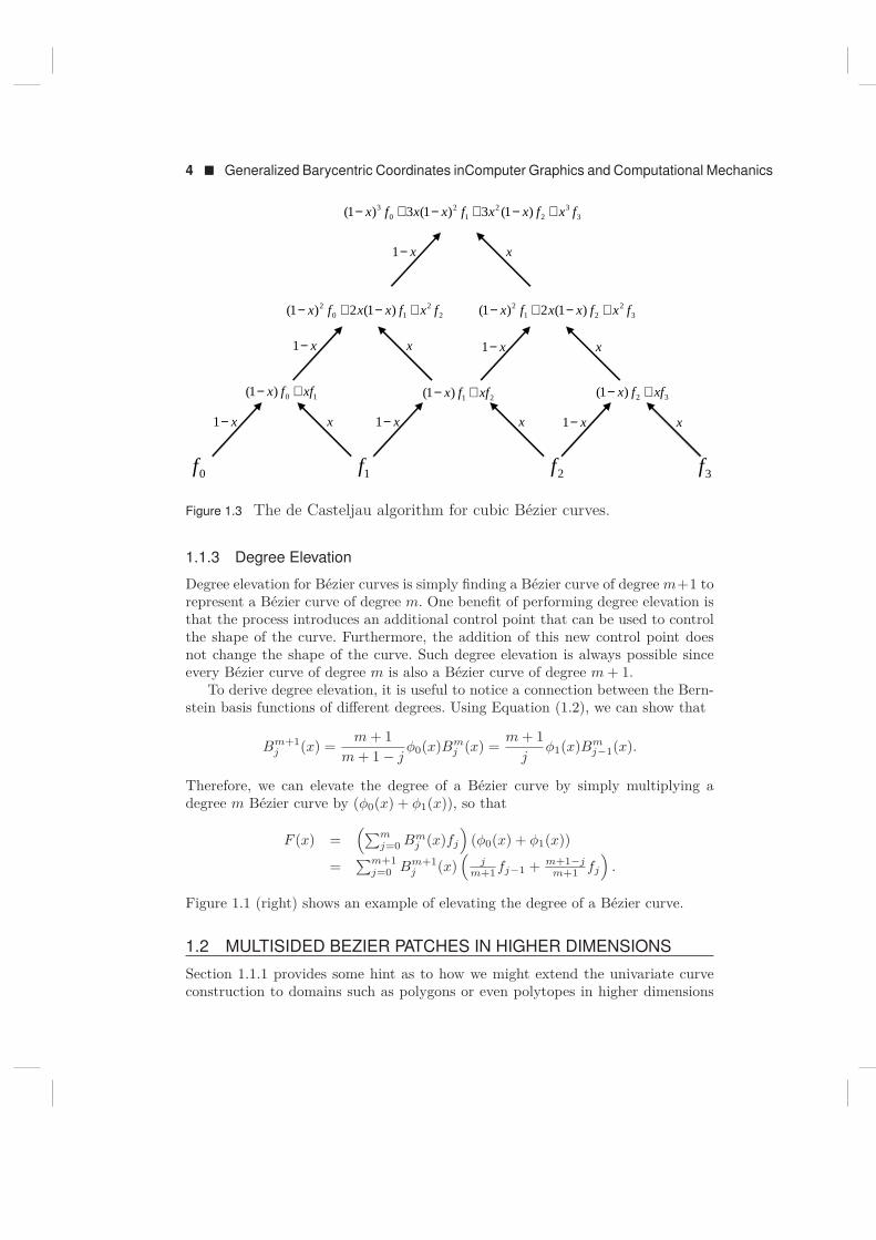
While we can evaluate Bezier curves by evaluating the polynomial expressions inthe Bernstein basis functions, a more elegant solution exists via de Casteljau’salgorithm. To do so, we introduce a graphical notation for a linear combination oftwo control points. Figure 1.2 shows a simple pyramid diagram. The arrows denotetaking the product of the value at the base of the arrow with the scalar value listedalong the arrow. The result of this product is then added to the sum at the endof the arrow. Hence, this figure denotes taking f0, f1 and multiplying these valuesby a, b respectively to form the result af0 + bf1. Using this notation, de Casteljau’salgorithm can be written in a very elegant fashion as a pyramid diagram shownin Figure 1.3 [3]. Note that each level of the pyramid produces lower order Bezierfunctions with the value of the curve appearing at the apex of the pyramid.


0f 1f 2f 3f

10)1( xffx +−21)1( xffx +− 32)1( xffx +−

22

102 )1(2)1( fxfxxfx +−+− 3

221

2 )1(2)1( fxfxxfx +−+−

33

22

12

03 )1(3)1(3)1( fxfxxfxxfx +−+−+−

x−1 x

xx−1

xx−1

xx−1

xx−1xx−1

Figure 1.3 The de Casteljau algorithm for cubic Bezier curves.

1.1.3 Degree Elevation

Degree elevation for Bezier curves is simply finding a Bezier curve of degree m+1 torepresent a Bezier curve of degree m. One benefit of performing degree elevation isthat the process introduces an additional control point that can be used to controlthe shape of the curve. Furthermore, the addition of this new control point doesnot change the shape of the curve. Such degree elevation is always possible sinceevery Bezier curve of degree m is also a Bezier curve of degree m + 1.

To derive degree elevation, it is useful to notice a connection between the Bern-stein basis functions of different degrees. Using Equation (1.2), we can show that

Bm+1j (x) = m + 1

m + 1 − jϕ0(x)Bm

j (x) = m + 1j

ϕ1(x)Bmj−1(x).

Therefore, we can elevate the degree of a Bezier curve by simply multiplying adegree m Bezier curve by (ϕ0(x) + ϕ1(x)), so that

F (x) =(∑m

j=0 Bmj (x)fj

)(ϕ0(x) + ϕ1(x))

=∑m+1

j=0 Bm+1j (x)

(j

m+1 fj−1 + m+1−jm+1 fj

).

Figure 1.1 (right) shows an example of elevating the degree of a Bezier curve.

1.2 MULTISIDED BEZIER PATCHES IN HIGHER DIMENSIONS

Section 1.1.1 provides some hint as to how we might extend the univariate curveconstruction to domains such as polygons or even polytopes in higher dimensions


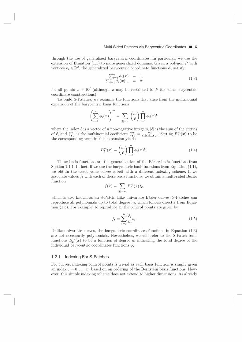
through the use of generalized barycentric coordinates. In particular, we use theextension of Equation (1.1) to more generalized domains. Given a polygon P withvertices vi ∈ Rd, the generalized barycentric coordinate functions ϕi satisfy∑n

i=1 ϕi(x) = 1,∑ni=1 ϕi(x)vi = x

(1.3)

for all points x ∈ Rd (although x may be restricted to P for some barycentriccoordinate constructions).

To build S-Patches, we examine the functions that arise from the multinomialexpansion of the barycentric basis functions(

n∑i=1

ϕi(x)

)m

=∑

|ℓ|=m

(m

ℓ

) n∏i=1

ϕi(x)ℓi

where the index ℓ is a vector of n non-negative integers, |ℓ| is the sum of the entriesof ℓ, and

(mℓ

)is the multinomial coefficient

(mℓ

)= m!

ℓ1!ℓ2!...ℓn! . Setting Bmℓ (x) to be

the corresponding term in this expansion yields

Bmℓ (x) =

(m

ℓ

) n∏i=1

ϕi(x)ℓi . (1.4)

These basis functions are the generalization of the Bezier basis functions fromSection 1.1.1. In fact, if we use the barycentric basis functions from Equation (1.1),we obtain the exact same curves albeit with a different indexing scheme. If weassociate values fℓ with each of these basis functions, we obtain a multi-sided Bezierfunction

f(x) =∑

|ℓ|=m

Bmℓ (x)fℓ,

which is also known as an S-Patch. Like univariate Bezier curves, S-Patches canreproduce all polynomials up to total degree m, which follows directly from Equa-tion (1.3). For example, to reproduce x, the control points are given by

fℓ =n∑

i=1

ℓi

mvi. (1.5)

Unlike univariate curves, the barycentric coordinates functions in Equation (1.3)are not necessarily polynomials. Nevertheless, we will refer to the S-Patch basisfunctions Bm

ℓ (x) to be a function of degree m indicating the total degree of theindividual barycentric coordinates functions ϕi.

1.2.1 Indexing For S-Patches

For curves, indexing control points is trivial as each basis function is simply givenan index j = 0, . . . , m based on an ordering of the Bernstein basis functions. How-ever, this simple indexing scheme does not extend to higher dimensions. As already


)20000( )02000(

)00200()00002(

)00020(

)10001(

)11000(

)01100(

)00110()00011(

)10100(

)10010(

)01001(

)00101(

)01010(

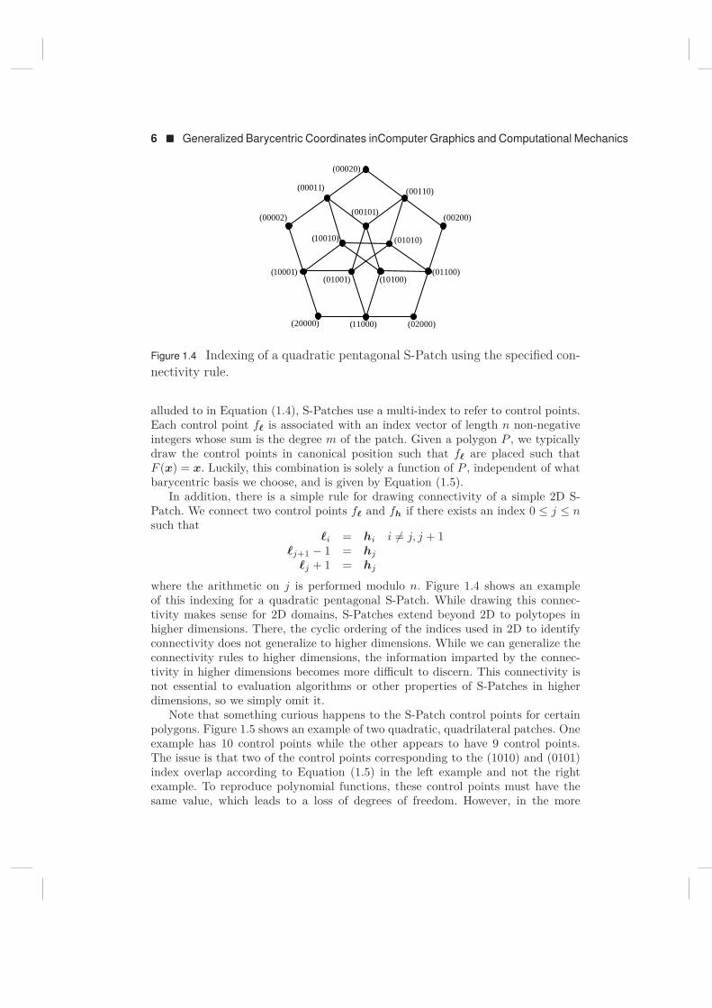
Figure 1.4 Indexing of a quadratic pentagonal S-Patch using the specified con-nectivity rule.

alluded to in Equation (1.4), S-Patches use a multi-index to refer to control points.Each control point fℓ is associated with an index vector of length n non-negativeintegers whose sum is the degree m of the patch. Given a polygon P , we typicallydraw the control points in canonical position such that fℓ are placed such thatF (x) = x. Luckily, this combination is solely a function of P , independent of whatbarycentric basis we choose, and is given by Equation (1.5).

In addition, there is a simple rule for drawing connectivity of a simple 2D S-Patch. We connect two control points fℓ and fh if there exists an index 0 ≤ j ≤ nsuch that

ℓi = hi i = j, j + 1ℓj+1 − 1 = hj

ℓj + 1 = hj

where the arithmetic on j is performed modulo n. Figure 1.4 shows an exampleof this indexing for a quadratic pentagonal S-Patch. While drawing this connec-tivity makes sense for 2D domains, S-Patches extend beyond 2D to polytopes inhigher dimensions. There, the cyclic ordering of the indices used in 2D to identifyconnectivity does not generalize to higher dimensions. While we can generalize theconnectivity rules to higher dimensions, the information imparted by the connec-tivity in higher dimensions becomes more difficult to discern. This connectivity isnot essential to evaluation algorithms or other properties of S-Patches in higherdimensions, so we simply omit it.

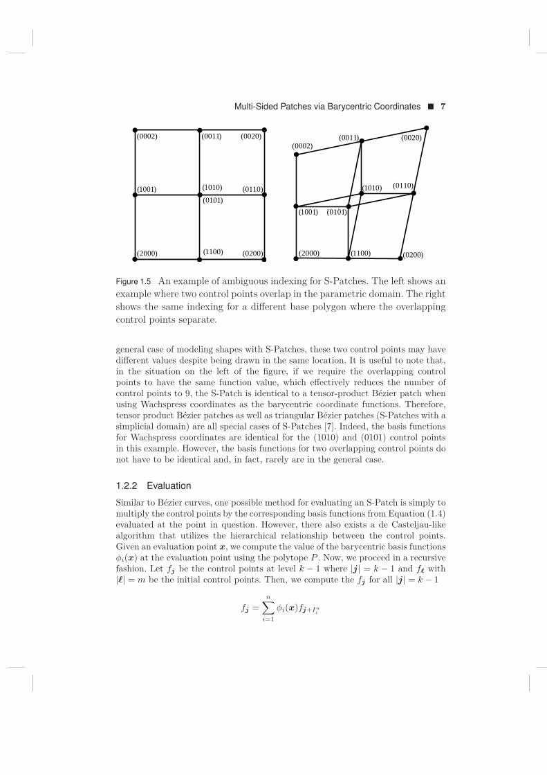
Note that something curious happens to the S-Patch control points for certainpolygons. Figure 1.5 shows an example of two quadratic, quadrilateral patches. Oneexample has 10 control points while the other appears to have 9 control points.The issue is that two of the control points corresponding to the (1010) and (0101)index overlap according to Equation (1.5) in the left example and not the rightexample. To reproduce polynomial functions, these control points must have thesame value, which leads to a loss of degrees of freedom. However, in the more


)2000( )1100( )0200(

)0101(

)1010( )0110(

)0020()0011()0002(

)1001(

)2000( )0200(

)0020()0002(

)1100(

)0110(

)0011(

)1001( )1010(

)0101(

Figure 1.5 An example of ambiguous indexing for S-Patches. The left shows anexample where two control points overlap in the parametric domain. The rightshows the same indexing for a different base polygon where the overlappingcontrol points separate.

general case of modeling shapes with S-Patches, these two control points may havedifferent values despite being drawn in the same location. It is useful to note that,in the situation on the left of the figure, if we require the overlapping controlpoints to have the same function value, which effectively reduces the number ofcontrol points to 9, the S-Patch is identical to a tensor-product Bezier patch whenusing Wachspress coordinates as the barycentric coordinate functions. Therefore,tensor product Bezier patches as well as triangular Bezier patches (S-Patches with asimplicial domain) are all special cases of S-Patches [7]. Indeed, the basis functionsfor Wachspress coordinates are identical for the (1010) and (0101) control pointsin this example. However, the basis functions for two overlapping control points donot have to be identical and, in fact, rarely are in the general case.

1.2.2 Evaluation

Similar to Bezier curves, one possible method for evaluating an S-Patch is simply tomultiply the control points by the corresponding basis functions from Equation (1.4)evaluated at the point in question. However, there also exists a de Casteljau-likealgorithm that utilizes the hierarchical relationship between the control points.Given an evaluation point x, we compute the value of the barycentric basis functionsϕi(x) at the evaluation point using the polytope P . Now, we proceed in a recursivefashion. Let fj be the control points at level k − 1 where |j| = k − 1 and fℓ with|ℓ| = m be the initial control points. Then, we compute the fj for all |j| = k − 1

fj =n∑

i=1ϕi(x)fj+In

i


)(0

xφ )(1

xφ

)(2

xφ)(

3xφ

)(4

xφ

)10000(f

)20000(f )11000(f

)10100(f

)10010(f

)10001(f)(

0xφ )(

1xφ

)(2

xφ)(

3xφ

)(4

xφ

)00000(f

)10000(f)01000(f

)00100(f

)00010(f

)00001(f

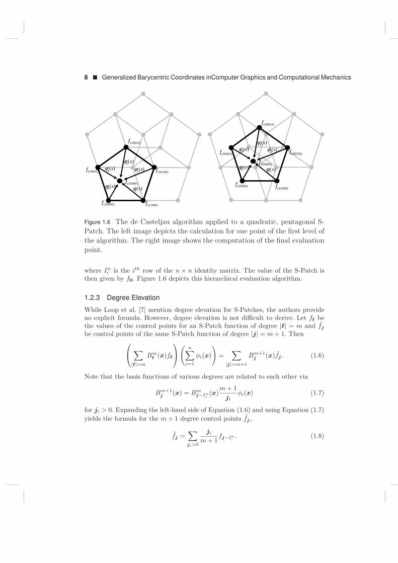
Figure 1.6 The de Casteljau algorithm applied to a quadratic, pentagonal S-Patch. The left image depicts the calculation for one point of the first level ofthe algorithm. The right image shows the computation of the final evaluationpoint.

where Ini is the ith row of the n × n identity matrix. The value of the S-Patch is

then given by f0. Figure 1.6 depicts this hierarchical evaluation algorithm.

1.2.3 Degree Elevation

While Loop et al. [7] mention degree elevation for S-Patches, the authors provideno explicit formula. However, degree elevation is not difficult to derive. Let fℓ bethe values of the control points for an S-Patch function of degree |ℓ| = m and fj

be control points of the same S-Patch function of degree |j| = m + 1. Then ∑|ℓ|=m

Bmℓ (x)fℓ

( n∑i=1

ϕi(x)

)=

∑|j|=m+1

Bm+1j (x)fj . (1.6)

Note that the basis functions of various degrees are related to each other via

Bm+1j (x) = Bm

j−Ini

(x)m + 1ji

ϕi(x) (1.7)

for ji > 0. Expanding the left-hand side of Equation (1.6) and using Equation (1.7)yields the formula for the m + 1 degree control points fj ,

fj =∑ji>0

ji

m + 1fj−In

i. (1.8)


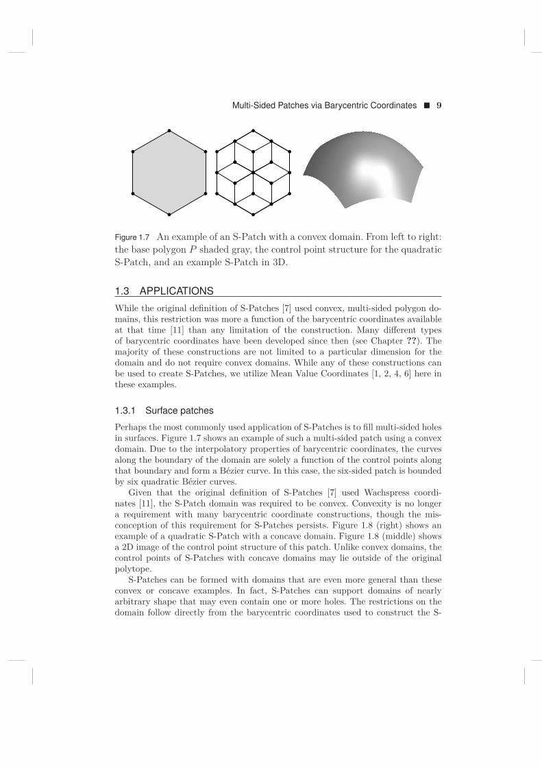
Figure 1.7 An example of an S-Patch with a convex domain. From left to right:the base polygon P shaded gray, the control point structure for the quadraticS-Patch, and an example S-Patch in 3D.

1.3 APPLICATIONS

While the original definition of S-Patches [7] used convex, multi-sided polygon do-mains, this restriction was more a function of the barycentric coordinates availableat that time [11] than any limitation of the construction. Many different typesof barycentric coordinates have been developed since then (see Chapter ??). Themajority of these constructions are not limited to a particular dimension for thedomain and do not require convex domains. While any of these constructions canbe used to create S-Patches, we utilize Mean Value Coordinates [1, 2, 4, 6] here inthese examples.

1.3.1 Surface patches

Perhaps the most commonly used application of S-Patches is to fill multi-sided holesin surfaces. Figure 1.7 shows an example of such a multi-sided patch using a convexdomain. Due to the interpolatory properties of barycentric coordinates, the curvesalong the boundary of the domain are solely a function of the control points alongthat boundary and form a Bezier curve. In this case, the six-sided patch is boundedby six quadratic Bezier curves.

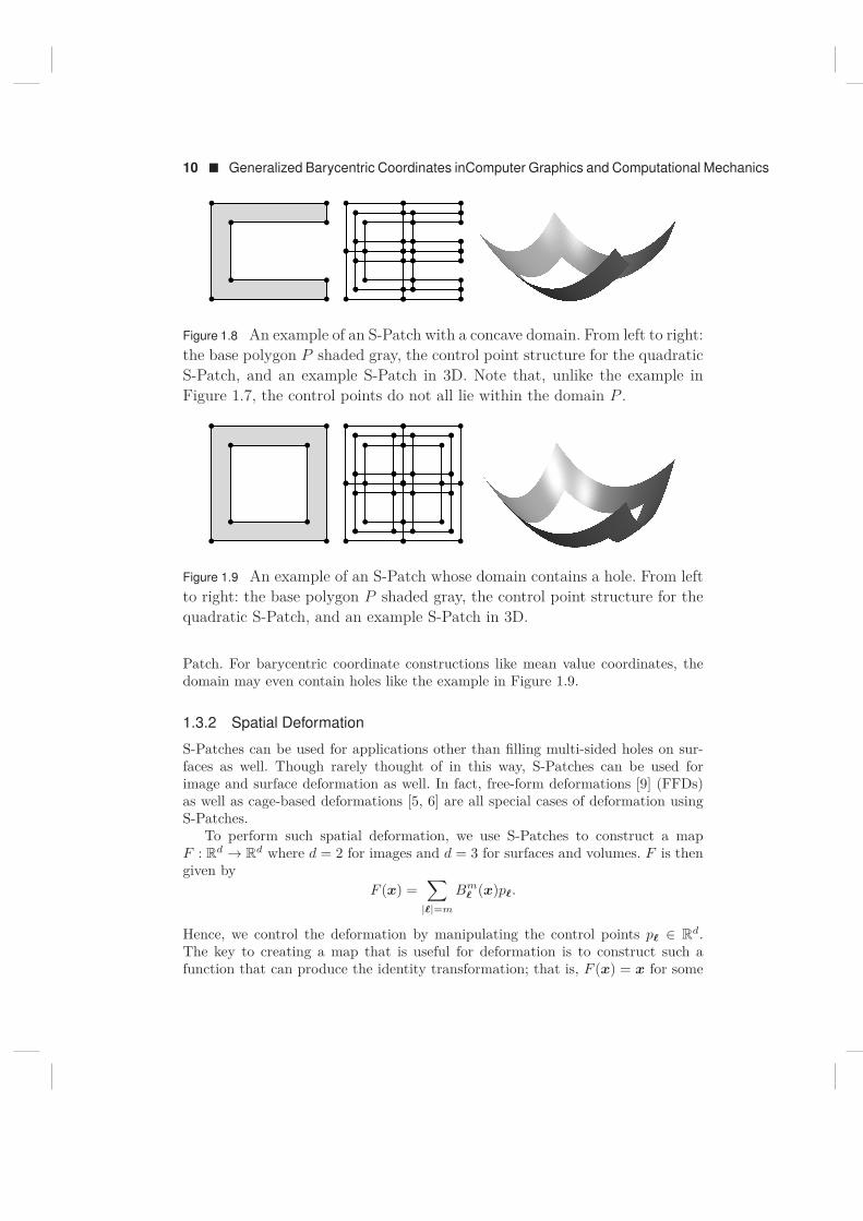
Given that the original definition of S-Patches [7] used Wachspress coordi-nates [11], the S-Patch domain was required to be convex. Convexity is no longera requirement with many barycentric coordinate constructions, though the mis-conception of this requirement for S-Patches persists. Figure 1.8 (right) shows anexample of a quadratic S-Patch with a concave domain. Figure 1.8 (middle) showsa 2D image of the control point structure of this patch. Unlike convex domains, thecontrol points of S-Patches with concave domains may lie outside of the originalpolytope.

S-Patches can be formed with domains that are even more general than theseconvex or concave examples. In fact, S-Patches can support domains of nearlyarbitrary shape that may even contain one or more holes. The restrictions on thedomain follow directly from the barycentric coordinates used to construct the S-


Figure 1.8 An example of an S-Patch with a concave domain. From left to right:the base polygon P shaded gray, the control point structure for the quadraticS-Patch, and an example S-Patch in 3D. Note that, unlike the example inFigure 1.7, the control points do not all lie within the domain P .

Figure 1.9 An example of an S-Patch whose domain contains a hole. From leftto right: the base polygon P shaded gray, the control point structure for thequadratic S-Patch, and an example S-Patch in 3D.

Patch. For barycentric coordinate constructions like mean value coordinates, thedomain may even contain holes like the example in Figure 1.9.

1.3.2 Spatial Deformation

S-Patches can be used for applications other than filling multi-sided holes on sur-faces as well. Though rarely thought of in this way, S-Patches can be used forimage and surface deformation as well. In fact, free-form deformations [9] (FFDs)as well as cage-based deformations [5, 6] are all special cases of deformation usingS-Patches.

To perform such spatial deformation, we use S-Patches to construct a mapF : Rd → Rd where d = 2 for images and d = 3 for surfaces and volumes. F is thengiven by

F (x) =∑

|ℓ|=m

Bmℓ (x)pℓ.

Hence, we control the deformation by manipulating the control points pℓ ∈ Rd.The key to creating a map that is useful for deformation is to construct such afunction that can produce the identity transformation; that is, F (x) = x for some


( )32

54 ,

22 )1()1( vu −− 2)1()1(2 vuu −− 22 )1( vu −

22vu22)1( vu− 2)1(2 uvu−

vvu )1()1(2 2 −− vvu )1(2 2 −vvuu )1()1(4 −−

l

p( )32

54 ,

2251

2258

22516

2254

22532

22564

2254

22532

22564

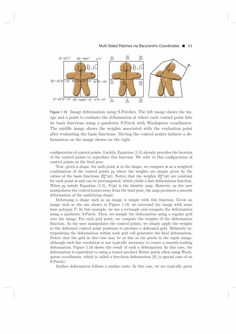
Figure 1.10 Image deformation using S-Patches. The left image shows the im-age and a point to evaluate the deformation at where each control point listsits basis functions using a quadratic S-Patch with Wachspress coordinates.The middle image shows the weights associated with the evaluation pointafter evaluating the basis functions. Moving the control points induces a de-formation on the image shown on the right.

configuration of control points. Luckily, Equation (1.5) already provides the locationof the control points to reproduce this function. We refer to this configuration ofcontrol points as the bind pose.

Now, given a shape, for each point x in the shape, we compute x as a weightedcombination of the control points pℓ where the weights are simply given by thevalues of the basis functions Bm

ℓ (x). Notice that the weights Bmℓ (x) are constant

for each point x and can be precomputed, which yields a fast deformation function.When pℓ satisfy Equation (1.5), F (x) is the identity map. However, as the usermanipulates the control points away from the bind pose, the map produces a smoothdeformation of the underlying shape.

Deforming a shape such as an image is simple with this function. Given animage such as the one shown in Figure 1.10, we surround the image with somebase polygon P . In this example, we use a rectangle and compute the deformationusing a quadratic S-Patch. Then, we sample the deformation using a regular gridover the image. For each grid point, we compute the weights of the deformationfunction. As the user manipulates the control points, we simply apply the weightsto the deformed control point positions to produce a deformed grid. Bilinearly in-terpolating the deformation within each grid cell generates the final deformation.Notice that the grid in this case may be as fine as the pixels in the input image,although such fine resolution is not typically necessary to create a smooth-lookingdeformation. Figure 1.10 shows the result of such a deformation. In this case, thedeformation is equivalent to using a tensor-product Bezier patch when using Wach-spress coordinates, which is called a free-form deformation [9] (a special case of anS-Patch).

Surface deformation follows a similar route. In this case, we are typically given


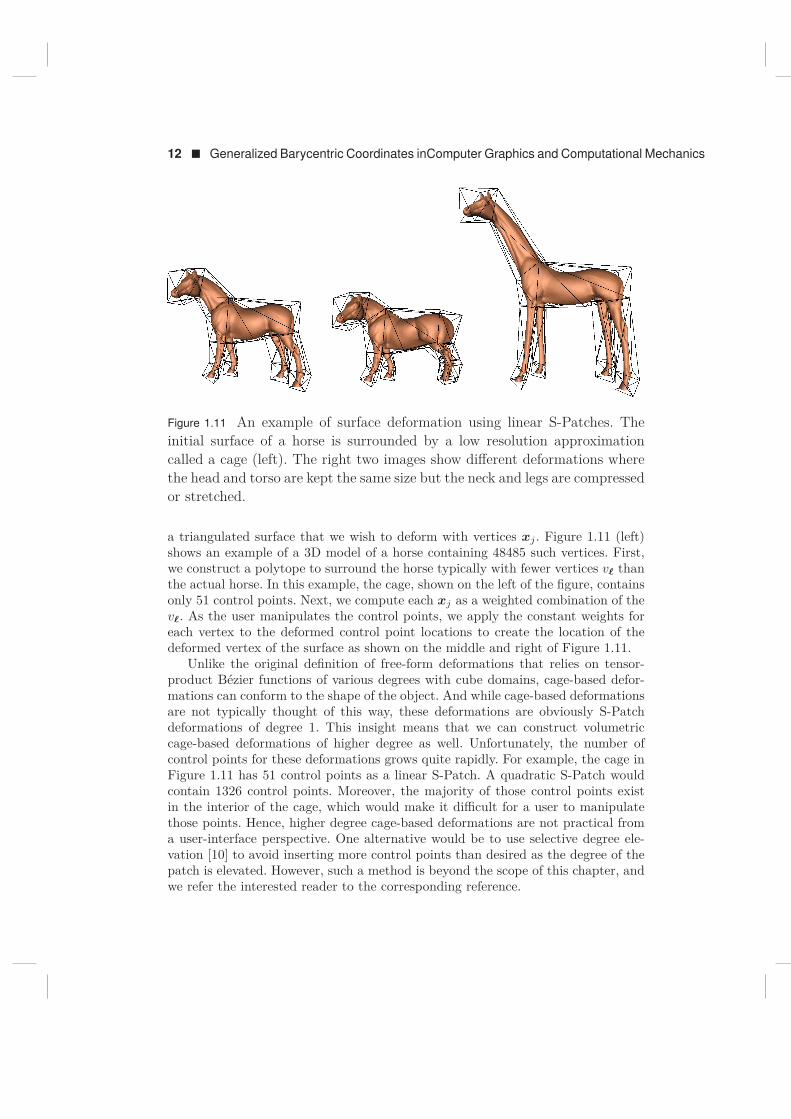
Figure 1.11 An example of surface deformation using linear S-Patches. Theinitial surface of a horse is surrounded by a low resolution approximationcalled a cage (left). The right two images show different deformations wherethe head and torso are kept the same size but the neck and legs are compressedor stretched.

a triangulated surface that we wish to deform with vertices xj . Figure 1.11 (left)shows an example of a 3D model of a horse containing 48485 such vertices. First,we construct a polytope to surround the horse typically with fewer vertices vℓ thanthe actual horse. In this example, the cage, shown on the left of the figure, containsonly 51 control points. Next, we compute each xj as a weighted combination of thevℓ. As the user manipulates the control points, we apply the constant weights foreach vertex to the deformed control point locations to create the location of thedeformed vertex of the surface as shown on the middle and right of Figure 1.11.

Unlike the original definition of free-form deformations that relies on tensor-product Bezier functions of various degrees with cube domains, cage-based defor-mations can conform to the shape of the object. And while cage-based deformationsare not typically thought of this way, these deformations are obviously S-Patchdeformations of degree 1. This insight means that we can construct volumetriccage-based deformations of higher degree as well. Unfortunately, the number ofcontrol points for these deformations grows quite rapidly. For example, the cage inFigure 1.11 has 51 control points as a linear S-Patch. A quadratic S-Patch wouldcontain 1326 control points. Moreover, the majority of those control points existin the interior of the cage, which would make it difficult for a user to manipulatethose points. Hence, higher degree cage-based deformations are not practical froma user-interface perspective. One alternative would be to use selective degree ele-vation [10] to avoid inserting more control points than desired as the degree of thepatch is elevated. However, such a method is beyond the scope of this chapter, andwe refer the interested reader to the corresponding reference.

Bibliography

[1] M. S. Floater. Mean value coordinates. Computer Aided Geometric Design,20(1):19–27, Mar. 2003.

[2] M. S. Floater, G. Kos, and M. Reimers. Mean value coordinates in 3D. Com-puter Aided Geometric Design, 22(7):623 – 631, 2005.

[3] R. Goldman. Pyramid Algorithms : A Dynamic Programming Approach toCurves and Surfaces for Geometric Modeling. Morgan Kaufmann, San Fran-cisco (Calif.), 2003.

[4] K. Hormann and M. S. Floater. Mean value coordinates for arbitrary planarpolygons. ACM Transactions on Graphics, 25(4):1424–1441, Oct. 2006.

[5] P. Joshi, M. Meyer, T. DeRose, B. Green, and T. Sanocki. Harmonic coordi-nates for character articulation. ACM Transactions on Graphics, 26(3):Article71, 9 pages, July 2007. Proceedings of SIGGRAPH 2007.

[6] T. Ju, S. Schaefer, and J. Warren. Mean value coordinates for closed tri-angular meshes. ACM Transactions on Graphics, 24(3):561–566, July 2005.Proceedings of SIGGRAPH 2005.

[7] C. T. Loop and T. D. DeRose. A multisided generalization of Bezier surfaces.ACM Transactions on Graphics, 8(3):204–234, July 1989.

[8] L. Ramshaw. Blossoming: A Connect-the-dots Approach to Splines. DigitalSystems Research Center, 1987.

[9] T. W. Sederberg and S. R. Parry. Free-form deformation of solid geometricmodels. In Proceedings of SIGGRAPH, pages 151–160, 1986.

[10] J. Smith and S. Schaefer. Selective degree elevation for multi-sided Bézierpatches. Computer Graphics Forum, 34(2):609–615, 2015.

[11] E. L. Wachspress. A Rational Finite Element Basis, volume 114 of Mathematicsin Science and Engineering. Academic Press, New York, 1975.

13

generalized barycentric coordinates in computer...

Documents