HAL Id: hal-03340548https://hal.inria.fr/hal-03340548

Submitted on 10 Sep 2021

HAL is a multi-disciplinary open accessarchive for the deposit and dissemination of sci-entific research documents, whether they are pub-lished or not. The documents may come fromteaching and research institutions in France orabroad, or from public or private research centers.

L’archive ouverte pluridisciplinaire HAL, estdestinée au dépôt et à la diffusion de documentsscientifiques de niveau recherche, publiés ou non,émanant des établissements d’enseignement et derecherche français ou étrangers, des laboratoirespublics ou privés.

BaPCod - a generic branch-and-price codeRuslan Sadykov, François Vanderbeck

To cite this version:Ruslan Sadykov, François Vanderbeck. BaPCod - a generic branch-and-price code. [Technical Report]Inria Bordeaux Sud-Ouest. 2021. �hal-03340548�

BaPCod — a generic branch-and-price code

Ruslan Sadykov∗1,2 and Francois Vanderbeck3

1Bordeaux-Sud-Ouest Inria Research Centre, 200 avenue de laVieille Tour, 33405 Talence, France

2Institut de Mathematiques de Bordeaux, Universite de Bordeaux,351 cours de la Liberation, 33405 Talence, France

3Atoptima SAS, 16 place Sainte Eulalie, 33000 Bordeaux, France

September 10, 2021

Abstract

This document presents a user guide for BaPCod version 0.631, aC++ library implementing a generic branch-cut-and-price solver. We giveguidelines for installing BaPCod, using its modelling language, BaPCodparameterization, retrieving BaPCod statistics, and understanding BaP-Cod output. We also present the VRPSolver extension of BaPCod whichallows one to model and efficiently solve a large number of vehicle routingand related problems.

BaPCod was developed in Bordeaux University and Bordeaux Re-search Center of Inria, France.

∗Corresponding author: ruslan.sadykov@inria.fr1The most recent version of this user guide is available on the BaPCod website:

https://bapcod.math.u-bordeaux.fr

1

Contents

1 Introduction 31.1 Code structure . . . . . . . . . . . . . . . . . . . . . . . . . . . . 41.2 Compiling BaPCod and running demos . . . . . . . . . . . . . . 41.3 Creating a new application . . . . . . . . . . . . . . . . . . . . . 51.4 Running an application . . . . . . . . . . . . . . . . . . . . . . . 61.5 Citing BaPCod . . . . . . . . . . . . . . . . . . . . . . . . . . . . 6

2 Modelling language 72.1 Environment handler . . . . . . . . . . . . . . . . . . . . . . . . . 82.2 Model handler . . . . . . . . . . . . . . . . . . . . . . . . . . . . 82.3 Formulation handlers . . . . . . . . . . . . . . . . . . . . . . . . . 92.4 Variables and constraints . . . . . . . . . . . . . . . . . . . . . . 112.5 Objective function . . . . . . . . . . . . . . . . . . . . . . . . . . 122.6 Solution handler . . . . . . . . . . . . . . . . . . . . . . . . . . . 132.7 Branching . . . . . . . . . . . . . . . . . . . . . . . . . . . . . . . 142.8 Separation of cutting planes . . . . . . . . . . . . . . . . . . . . . 162.9 Pricing functor . . . . . . . . . . . . . . . . . . . . . . . . . . . . 17

3 BaPCod configuration 193.1 Main parameters . . . . . . . . . . . . . . . . . . . . . . . . . . . 193.2 Column generation parameters . . . . . . . . . . . . . . . . . . . 203.3 Cut generation parameters . . . . . . . . . . . . . . . . . . . . . . 223.4 Stabilization parameters . . . . . . . . . . . . . . . . . . . . . . . 233.5 Primal heuristic parameters . . . . . . . . . . . . . . . . . . . . . 243.6 Strong branching parameters . . . . . . . . . . . . . . . . . . . . 26

4 BaPCod statistics 284.1 Timers . . . . . . . . . . . . . . . . . . . . . . . . . . . . . . . . . 284.2 Records and counters . . . . . . . . . . . . . . . . . . . . . . . . 29

5 BaPCod output 30

6 VRPSolver extension 326.1 VRPSolver pricing functor . . . . . . . . . . . . . . . . . . . . . . 326.2 VRPSolver cut separation functors . . . . . . . . . . . . . . . . . 356.3 VRPSolver branching functors . . . . . . . . . . . . . . . . . . . 376.4 VRPSolver paramerization . . . . . . . . . . . . . . . . . . . . . . 386.5 VRPSolver output . . . . . . . . . . . . . . . . . . . . . . . . . . 40

7 Perspectives 42

2

1 Introduction

BaPCod is a prototype academic code that solves Mixed Integer Programs(MIP) by application of a Dantzig-Wolfe reformulation technique. The reformu-lated problem is solved using the branch-cut-and-price algorithm which includesthe column generation procedure to solve the linear relaxation in each node ofthe branch-and-bound tree. The specificity of this prototype is to offer a “black-box” implementation of the method:

1. the input is the set of constraints and variables of the MIP in its natural/compact formulation;

2. the user specifies which of these constraints and variables define the sub-systems on which the decomposition is based (it is handy to test differentdecompositions);

3. the reformulation is automatically generated by the code, without anyinput from the user to define master columns, their reduced cost, pricingproblem, or Lagrangian bound;

4. a default column generation procedure is implemented that relies on anunderlying LP/MIP solver to handle master and subproblem but the usercan define a specific solver for the pricing problem;

5. a branching scheme that preserves the pricing problem structure is offeredby default, it runs based on priorities and directives specified by the useron the original variables;

6. the user can specify custom cut generation callbacks and custom branchingcallbacks;

7. preprocessing, restricted master and diving primal heuristics, some stabi-lization techniques, and strong branching are available for use;

8. VRPSolver extension can optionally be used, which includes a resourceconstrained shortest path problem (RCSP) solver, and some families ofrobust and non-robust cut separation and branching functors; these com-ponents can be used to devise state-of-the-art branch-cut-and-price algo-rithms for vehicle routing and related problems.

Readers of this user guide are supposed to be familiar with the theoryof Dantzig-Wolfe reformulations, the column generation procedure, and thebranch-cut-and-price method (see for example [3] for an introduction).

The source code of BaPCod can be obtained on its web-page https://

bapcod.math.u-bordeaux.fr after accepting the Inria licence for academic use.The VRPSolver extension in the compiled form is available by request. Thefollowing contacts can be used to communicate with the authors of the code:

ruslan.sadykov@inria.fr — issues with the code, critical bugs, user guide,general issues;

laurent.facq@math.u-bordeaux.fr — issues with installation and runningof demos.

3

1.1 Code structure

We suppose that the code is cloned or extracted to the BapcodFramework folder.The main folder structure is the following

BapcodFramework

-- Applications

-- Bapcod

-- CMake

-- CMakeLists.txt

-- Demos

-- LICENCE.pdf

-- README.md

-- Scripts

-- Tools

Applications folder should contain user applications, no applications areprovided by default. We explain how to create an application in Section 1.3.Bapcod folder contains the C++ source code of BaPCod. Cmake folder andfile CMakeLists.txt contain CMake scripts necessary for compiling and linkingBaPCod, its demos and user applications. Demo folder contains demos whichcome together with BaPCod source code. LICENCE.pdf and README.md files con-tain the licence and the installation instructions. The licence stipulates that youcan use BaPCod for free for academic purposes. Scripts folder contains somescripts necessary for BaPCod installation and other tasks. Tools folder con-tains the archived source code of two third-party open-source libraries, namelyBoost 1.76 and LEMON 1.3.1. BaPCod is dependent on these libraries. Theselibraries should be compiled before compiling BaPCod, see Section 1.2. BaP-Cod also depends on Cplex library, which can be obtained for free for academicuse.

1.2 Compiling BaPCod and running demos

Those are the minimum requirements to compile and run demos and applicationsdependent on BaPCod:

• CMake version 3.12 and above;

• Boost version 1.76 (included with the BaPCod distribution in Tools folder);

• LEMON version 1.3.1 (included with the BaPCod distribution in Tools

folder);

• Cplex version 12.8 and above.

First, make sure that CMake and Cplex are installed. To install Boost andLEMON, in terminal, run the following commands from the BapcodFramework

folder.

bash Scripts/shell/install_bc_lemon.sh

bash Scripts/shell/install_bc_boost.sh

4

If you want to use the VRPSolver extension, you need to request RCSPlibrary (available for Linux and Mac OS) distributed in librcsp.tgz archive,and then extract it to BapcodFramework/Tools/rcsp folder (please be sure thatyou obtain folder BapcodFramework/Tools/rcsp/include with header files andfolder BapcodFramework/Tools/rcsp/lib with the library file).

Now you are ready to compile BaPCod. For that, run the following com-mands from the BapcodFramework folder

mkdir build

cd build

cmake -DCMAKE_BUILD_TYPE=Release ..

make -j bapcod

To test installation, you can run a demo distributed with BaPCod. Forexample to run VertexColoring demo, run the following commands from theBapcodFramework folder

cd build/Demos/VertexColoring

make -j

bash tests/runTests.sh

1.3 Creating a new application

A demo or an application has the following structure by default

<ApplicationOrDemoName>

-- CMake

-- CMakeLists.txt

-- config

-- data

-- include

-- src

-- tests

Cmake folder and file CMakeLists.txt contain CMake scripts necessary forcompiling and linking the application or demo. config folder contains config-uration files. There are usually two configuration files: one contains BaPCodparameters, and another contains application-specific parameters. data foldercontains instance files. include folder contains header files. src folder containssource files. tests folder contains files and scripts to run non-regression tests.It is highly advised to create several non-regression tests for every user applica-tion. Non-regression tests usually verify that the solution value obtained afterthe run coincides with the optimal value or the dual bound value.

A standard way to create a new application is by modification of a similaravailable demo. If there is no demo which is similar to the intended application,please request the authors of the code to produce a similar demo. One advantageof this method is to provide for the user a working tree that already containsthe files needed by cmake for the compilation and pre-filled configuration andtest files. Another advantage is to provide for the user the code structure thatis easier to modify when making up the new application rather than startingfrom scratch.

5

First, copy the folder with the corresponding demo to theBapcodFramework/Applications folder. Then modify the folder name to theapplication name, and add the new folder name to fileBapcodFramework/Applications/CMakeLists.txt inside add_subdirectories()so that the makefile is produced next time your run cmake.

Afterwards, the code of the new application should be modified accordingto the problem one wants to solve. It is advised to change the names of allclasses in the application code or to change the name of the namespace used inthe code, in order to avoid a clash between different demos and applications.Usually, to adapt the code to the new application, one should change the classwith application-specific parameters, the data class, functions to read the data,the model and the callbacks (pricing, cut generation, branching), if applicable.

After the code modification is complete, the makefile of the applicationshould be generated. For that, run the following commands from the BapcodFrameworkfolder

cd build

cmake ..

These commands should also be run each time you add or delete header orsource files for an application.

1.4 Running an application

To run the application, execute the following commands from the BapcodFrameworkfolder

cd build/Applications/<AppName>

make -j

bin/<AppName> -b <BaPCod_config> -a <app_config> -i <instance>

Here <AppName> is the name of the application, <BaPCod_config> is the (rela-tive) path to the configuration file with BaPCod parameters, <app_config> isthe (relative) path to the configuration file with application-specific parameters(if such parameters exists), and <instance> is the (relative) path to the dateinstance file. You can specify additional BaPCod and application-specific pa-rameters in the command line using the format --<paramName> <value> . Ifdifferent values are given for the same parameter in the configuration file andin the command line, the value given in the command line has more priority.See Section 3 for an overview of BaPCod parameters. In addition, in the com-mand line one can specify -t <tree_file> parameter to change the default(relative) path (which is BaPTree.dot) to the file where the branch-and-boundtree information will be stored in .DOT format for later visualisation.

It is highly advised to use a version control system (for example Git) foruser applications. It is standard to create a different repository for every userapplication.

1.5 Citing BaPCod

If you use BaPCod, please cite the present document. In addition, if you use thefollowing components of BaPCod, we encourage you to cite the correspondingpapers listed below.

6

• If you use stabilization (automatic dual price smoothing stabilization isactivated by default), please cite paper [11]:Artur Pessoa, Ruslan Sadykov, Eduardo Uchoa, and Francois Vanderbeck.Automation and combination of linear-programming based stabilizationtechniques in column generation. INFORMS Journal on Computing,30(2):339–360, 2018.

• If you use primal heuristics, please cite paper [17]:Ruslan Sadykov, Francois Vanderbeck, Artur Pessoa, Issam Tahiri, andEduardo Uchoa. Primal heuristics for branch-and-price: the assets ofdiving methods. INFORMS Journal on Computing, 31(2):251–267, 2019.

• If you use the VPRSolver extension, please cite paper [12]:Artur Pessoa, Ruslan Sadykov, Eduardo Uchoa, and Francois Vanderbeck.A generic exact solver for vehicle routing and related problems. Mathe-matical Programming, 183:483–523, 2020.

2 Modelling language

This section overviews the modelling language, i.e. the C++ interface for BaP-Cod. To use this interface, one needs to include the corresponding header file:

#include "bcModelingLanguageC.hpp"

BaPCod models are similar to Mixed Integer Programs (MIPs): the userneeds to define (continuous or integer) variables, linear constraints and theobjective function. Models are defined using of original variables, i.e. variablesof the original compact formulation. There are however following differences.

The user needs to specify the decomposition: i.e. which constraints are du-alized (remain in the master formulation) and which constraints are imposedwhen solving the subproblem formulations (or pricing problems). Therefore, atleast two formulations should be defined: master one and at least one subprob-lem formulation. Each subproblem formulations has integer bounds specifyinghow many solutions of this subproblem (i.e. how many columns generated bythis pricing problem) can participate in the global solution of the model. Thesebounds are useful to define identical subproblems.

Using BaPCod without defining a subproblem formulation is possible whenone wants to solve the original formulation by the MIP solver. This may beuseful when benchmarking a decomposition against the original formulation.

Each variable belongs to a formulation. Subproblem constraints may involveonly variables belonging to the corresponding subproblem formulation. On thecontrary, master constraints may involve variables belonging both to the masterformulation (we call them pure master variables) and to the subproblem formu-lations. Coefficients of subproblem variables in the master constraints determinethe coefficients of columns in these constraints.

The user has a possibility to define additional functors (C++ classes) toimprove the performance of BaPCod. Functors are enhanced versions of call-backs. A functor may have several functions which are called in different stagesof the solution process. The main functor is the pricing one which may bedefined for a subproblem formulation for managing the corresponding pricing

7

problem. Another important functor is to separate robust cutting planes. Suchcutting planes are defined similarly to standard constraints using original vari-ables. The user can also define a functor for generation of robust branchingconstraints. Defining non-robust cutting plains and branching constraints isalso possible but reserved for an advanced use. The VRPSolver extension pre-defines a certain number of functors which are used for solving vehicle routingand related problems. This extension is reviewed in Section 6.

2.1 Environment handler

Every time BaPCod is used, one should first declare an environment handler oftype BcInitialisation using constructor

BcInitialisation(int argc , char *argv[],

std:: string config_filename = "config/bcParams.cfg");

Here argc and argv are the standard parameters of the main() function forcommand line arguments, and config_filename is the default (relative) pathto the configuration file with BaPCod parameters (for the case -b parameterdoes not present in the command line).

The environment handler has several useful methods.

UserControlParameters & param ();

This method allows one to obtain the object with basic BaPCod parameterswhich can be used to get values of these parameters.

void bcReset ();

This method should necessarily be called between two calls to BcModel::solve()function (of a model associated with this environment handler) in order to resetinternal counters.

Finally, for obtaining the statistics of the execution on can use the methods

double getStatisticValue(const std:: string & statName );

long getStatisticCounter(const std:: string & statName );

double getStatisticTime(const std:: string & statName );

to get values of individual statistics (records, counters, and timers). See Sec-tion 4 for an overview of BaPCod statistics.

2.2 Model handler

The model handler is used to define and solve BaPCod models. Every modelshould be associated with a BaPCod environment handler, specified in the modelconstructor:

BcModel(const BcInitialisation & bapcodInit ,

const std:: string & modelName = "Model");

8

The main method of the handler solves the model:

BcSolution solve ();

It returns the best found solution. The solution returned is disaggregated bydefault, see Section 2.6 for details.

Solution management callback can be attached to a model:

void attach(BcSolutionFoundCallback * solutionFoundCallbackPtr );

This callback is called every time a solution is found which is considered to befeasible by the model. This callback can be used to check the feasibility of thesolution (and thus the correctness of the model) and possibly show and/or storeit for future use.

2.3 Formulation handlers

Formulation handler BcFormulation serves to manage formulations. In themodelling interface of BaPCod, formulations are handled in arrays. BcMasterArrayis the array of master formulations (although only the first one is used), andBcColGenSpArray is an array of subproblem formulations, both inherit fromBcFormulationArray. Formulation arrays should belong to a model, thus theconstructors for their definition are the following

BcMasterArray(BcModel & model , const std:: string & name = "master");

BcColGenSpArray(BcModel & model , const std:: string & name = "colGenSp");

BcFormulationArray has two operators operator() and operator[] toaccess individual formulations in the array. These operators take integer indicesas parameters. The first operator creates the formulation with given indicesif it does not exists. If no index is given, 0 is used by default. The secondoperator does not create formulation; if the formulation with given indices doesnot exist, an error occurs. For example, the following code creates a model withthe master formulation and two subproblem formulations.

BcInitialisation bcInit(argc , argv);

BcModel model(bcInit );

BcMasterArray master(model);

master ();

BcColGenSpArray colGenSp(model);

colGenSp (0);

colGenSp (1);

The master formulation of a subproblem one can be obtained with method

const BcMaster BcFormulation :: master () const;

It returns BcMaster handler which inherits from BcFormulation. If the formu-lation is not a subproblem one, the returned master formulation is not defined.

9

The same method, defined for BcModel, allows one to retrieve the master for-mulation of a model.

The list of subproblem formulations of a master one can be obtained withmethod

const std::list < BcFormulation > & colGenSubProblemList () const;

If the formulation is not the master one, the returned list is empty.For a subproblem formulation, one may define multiplicity bounds, i.e. the

minimum and maximum number of solutions (i.e. columns) from this formu-lation which can participate in the global model solution. These bounds willdefine convexity constraints in the restricted master problem. The bounds areset with operators operator>=, operator<=, and operator==. For example,the code

colGenSp [0] >= 1;

colGenSp [1] <= 2;

sets lower bound one for the subproblem formulation with index 0 (by default,the lower bound is equal to 0), and upper bound two for the subproblem for-mulation with index 1 (by default, the upper bound is equal to ∞).

For a subproblem formulation, one may also define the fixed cost, i.e. thevalue which will be added to the coefficient in the objective function of everycolumn coming from this subproblem. The method is

void BcFormulation :: setFixedCost(const double & value);

By default, the fixed cost is equal to zero. For example, in the bin packingmodel, the fixed cost of the knapsack subproblem may be set to 1.0. The samesetFixedCost method is defined for BcColGenSpArray. It sets the same fixedcost for all subproblem formulations in the array.

The master formulation can be initialized with a set of columns using twomethods of BcMaster (which can be obtained by BcMaster(master())):

const BcFormulation & operator +=( BcSolution & sol);

void initializeWithColumns(BcSolution & sol , BcDualSolution * dualSol );

These two methods should be called after completely defining the master andsubproblem formulations. The solution passed should be disaggregated (seeSection 2.6). The first operator updates the global solution of the model andadds its subproblem solutions as columns to the restricted master problem (ifparameterized accordingly, see Section 3.2). The second method adds columnscorresponding to subproblem solutions in the provided solution chain sol to therestricted master problem (independently of the parameterization and withoutupdating the global solution of the model). Argument dualSol should be setto nullptr.

10

2.4 Variables and constraints

Variables and constraints are defined using arrays:

BcVarArray(const BcFormulation & formulation , const std:: string & name);

BcConstrArray(const BcFormulation & formulation , const std:: string & name = "");

Every array of variables or constraints should belong to a formulation, either tothe master or the a subproblem one. Note that these constructors are used intwo ways. First, one can create a new array of variables or constraints beforesolving the model. After starting the solution process, one can retrieve theexisting array by passing its name as the parameter. This functionality is usedto retrieve existing variables and constraints in user-defined functors.

The same operators operator() and operator[] as for formulations areused to access individual elements in the array. Again, the first operator createsthe element with given indices if it does not exist, the second operation raisesan error in this case. Note that the syntax of these operators is different formulti-dimensional indices:

BcVarArray xVar(colGenSp [0], "X");

xVar (0 ,0);

xVar [0][0] <= 1;

This code creates variable x0,0 belonging to the subproblem formulation withindex 0, and then sets the upper bound of this variable to 1. The type ofindividual variables is BcVar, and the type of individual constraints is BcConstr.

For an array of variables or constraints, one can define index characters:

xVar.defineIndexNames(MultiIndexNames(’i’,’j’));

This characters are used in names of individual variables. For example, thename of variable xVar[0][0] will be "Xi0j0".

For an array of variables, their type is set using method type:

xVar.type(’B’);

’B’ stands for binary, ’I’ for integer, and ’C’ for continuous. By default, vari-ables are continuous. The same method is also defined for individual variables.

For an array of variables, or individual variables, one can define their boundsusing operators operator<= and operator>=. For subproblem variables thesebounds are local and valid only when solving the subproblem. In the globalmodel solution, the total value of a subproblem variable can violate its localbounds. To set global bounds on subproblem variables, one should define thecorresponding master constraints.

For an array of constraints, or individual constraints, one can define theirsense and right-hand size using operators operator<=, operator>=, and operator==.For example the code

BcConstrArray setPackConstr(master(), "SPC");

setPackConstr (0) <= 1;

11

creates a less-or-equal constraint with the right-hand-size value equal to 1.For an array of constraints, or individual constraints, one can indicate whether

they will be used in preprocessing, using method

void toBeUsedInPreprocessing(bool flag);

To set coefficients of variables in constraints, one may use operators operator+=,operator+, operator-=, and operator-. For example, the code

BcConstrArray setCovConstr(master(), "SCC");

setCovConstr.defineIndexNames(MultiIndexNames(’k’));

setCovConstr (0) >= 2;

BcVarArray yVar(master(), "Y");

setCovConstr [0] += xVar [0][0] + 2 * y[0];

setCovConstr [0] -= 0.5 * xVar [0][0];

defines constraint 12x0,0 + 2y0 ≥ 2 with name "SCCk0".

2.5 Objective function

The objective functions are also handled in the array. Only the first objectivefunction is used. The objective array belongs to a model, its constructor is

BcObjectiveArray(BcModel & model , const std:: string & name = "objective")

The sense and integrality of the objective function is determined using themethod

void setMinMaxStatus(const BcObjStatus :: MinMaxIntFloat & newObjectiveSense );

Possible arguments are BcObjStatus::minInt and BcObjStatus::minFloat.One should avoid using maximization objective with BaPCod, as there areknown bugs when it is used. One can transform maximization objective to min-imization by multiplying it by −1. By default, the objective function is “float”,which mean it can take any value. If it is known that the objective functionvalue of any feasible solution is integer, one should give this information to thesolver by setting the objective function type to “integer”. In this case, the lowerbound will be rounded up before checking whether a branch-and-bound nodeshould be pruned, making the search tree smaller.

The objective function itself can be retrieved using operator operator().Coefficients of the variables in the objective function are set in the same way asfor constraints. For example, the code

BcObjectiveArray objective(model);

objective.setMinMaxStatus(BcObjStatus :: minInt );

objective () += yVar (0) + 2 * yVar (1);

sets the objective function to min y0+2y1 and states that it can take only integervalues. Both master and subproblem variables may participate in the objectivefunction.

The initial upper bound for the objective function value (i.e. the cut-offvalue) can be set using operator operator<=. For example, the code

12

objective () <= 100;

sets the cut-off value to 100, meaning that all branch-and-bound nodes will bepruned as soon as the lower bound becomes strictly greater than 99 (as theobjective function is known to be integer as indicated above). Setting initialupper bound to a value which is as close as possible to the optimum value isimportant to decrease the size of the search tree.

Another important method sets the initial coefficient of artificial variablesin the objective function:

void setArtCostValue(const double & guessVal );

In some cases, BaPCod may wrongly declare the model infeasible if the valueof this coefficient is below the optimum value. Therefore, a good practice isto set this coefficient to a known upper bound on the optimum solution value.Decreasing the value of this coefficient may help to avoid numerical issues whenthey are present.

2.6 Solution handler

In BaPCod modelling interface, solutions are stored using handlers of typeBcSolution. This handler may contain either a single solution or several solu-tions in a chain. The constructor of this handler is

BcSolution(const BcFormulation & formulation ,

const std:: string & solName = "Solution");

Each solution belongs to a formulation. A solution of a subproblem formu-lation defines the corresponding column in the restricted master problem. Toset a value of a variable in the solution, operators operator= and operator+=

is used. For example, the code

BcSolution bcSol(colGenSp [0]);

x[0][0] = 2;

bcSol += x[0][0];

defines a solution x0,0 = 2 (all other variables take value 0) for the subproblemformulation with index 0.

To add a solution to the solution chain, one can use method

BcSolution & appendSol(BcSolution & sol);

This method is useful, when one needs to pass several solutions. For example,the user-defined pricing problem solver may return several solutions so thatmultiple columns are added to the restricted master LP in a single columngeneration iteration.

To read all solutions in a solution chain, the following methods are useful:

13

BcSolution next() const;

bool defined () const;

One can obtain next solution in a loop until the current solution is not defined.To retrieve the variables with non-zero values in a solution, one can use

methods

const std::set < BcVar > & extractVar ();

const std::set < BcVar > & extractVar(const std:: string & genericName );

The first method retrieves all non-zero variables in the solution. The secondone retrieves only variables in the array with the given name. Once the non-zero variables are extracted, values of particular variables can be obtained usingmethod

double BcVar :: solVal () const;

Solutions of the master formulation can be standard (or aggregated) anddisaggregated. A standard solution has values of all variables, both masterand subproblem ones, in the aggregated form. This means that the value ofa subproblem variable in this solution is the weighted sum of values of thisvariable in solutions corresponding to columns, where weights are values of thecolumns in the master solution. A disaggregated solution is a chain of solutions,where the first solution contains values of pure master variables, and all othersolutions in the chain correspond to columns in the master solution. For everysuch solution in the chain, one can retrieve the subproblem solution it belongsto and its multiplicity, i.e. the value of the corresponding column in the mastersolution:

BcFormulation formulation () const;

int getMultiplicity () const;

By default, the solution returned by the solver is disaggregated.

2.7 Branching

One can use three types of branching in BaPCod: branching on variables,branching on constraints, and custom “algorithmic” branching (with user-definedfunctors).

To branch on variables, one needs to define their branching priorities. Forthat, the following methods exists for an array of variables

const BcVarArray & priorityForMasterBranching(double priorityValue );

const BcVarArray & priorityForSubproblemBranching(double priorityValue );

const BcVarArray & priorityForRyanFosterBranching(double priorityValue );

If the branching priority value is non-positive, the corresponding branchingstrategy is not applied. Default priority values for master branching, subprob-lem branching, and Ryan&Foster branching are 1.0, 0.1, and -1.0. The corre-sponding variable branching strategies are: 1) branching in master on the total

14

value of the variable; 2) Vanderbeck branching on bounds of subproblem vari-ables, proposed in [18]; 3) Ryan& Foster branching, proposed in [15]. It sufficesto use only the first branching strategy if the upper bound of all subproblemformulations is one, i.e. in the absence of identical subproblems. Otherwise, ifall subproblem variables are binary, Ryan& Foster branching may be used. Inthe most general case (identical subproblems with general integer subproblemvariables), the second branching strategy should be used to ensure the exactsolution. If the pricing functor is used for a subproblem, it should explicitlysupport Ryan& Foster branching in order to use it. The pricing functor needsto support arbitrary bounds on subproblem variables in order to use Vander-beck branching. Finally, we advise to use Vanderbeck branching only if it isreally needed, as we will not likely be able to correct possible bugs in the im-plementation. For variables which belong to the master formulation, only thefirst branching strategy is possible.

To branch on constraints, one should define array(s) of branching constraintsusing constructor

BcBranchingConstrArray(const BcFormulation & formulation ,

const std:: string & name ,

const SelectionStrategy & priorityRule

= SelectionStrategy :: MostFractional ,

const double & priorityLevel = 1.0);

Here the priorityLevel is the branching priority value of all constraints inthis array. After creating the array, branching constraints can be defined inthe same way as standard constraints, see Section 2.4. The only differenceis that the sense and the right-hand-size of branching constraints are ignored.Branching constraints are not added to the formulation in the beginning of thesolution process. During branching, the left-hand-side value v of each branchingconstraint is computed using the current solution of the restricted master LP.In the case v is fractional, two constraints with the same left-hand-size aregenerated for two child nodes of the branch-and-bound tree: one is less-or-equalto bvc, and the second is greater-or-equal to dve.

To add a custom “algorithmic” branching strategy one should define a func-tor which inherits from class BcDisjunctiveBranchingConstrSeparationFunctorand associate it to an array of branching constraints (such an array should notcontain any pre-defined branching constraints) using method

const BcBranchingConstrArray &

attach(BcDisjunctiveBranchingConstrSeparationFunctor

* separationRoutinePtr );

The functor should implement the following operator

bool operator ()( BcFormulation formPtr ,

BcSolution & primalSol ,

const int & candListMaxSize ,

std::list <std::pair <BcConstr , std::string >>

& retBrConstrList );

15

This function receives the master formulation handler, the solution handlerwhich contains the current solution of the restricted master LP, and the maxi-mum number of branching constraints which will be processed (others will be ig-nored). All branching constraints generated should be added to list retBrConstrListof pairs. The first member of the pair is the branching constraint generated, andthe second member is its description string. The description string is used torecognise the same branching constraint when collecting the branching history.The branching history is used to select good branching candidates in the strongbranching. In the function, the branching constraints should be defined in thesame way as above (their sense and right-hand-side are ignored). The functionshould return true if and only if at least one branching constraint has beenadded to retBrConstrList.

All defined branching strategies are applied in decreasing order of theirbranching priority values. If no branching candidate is found for branchingstrategies with a certain priority value, strategies with the next lower priorityvalue will be tried. If strong branching is used (see Section 3.6 for parameter-ization), branching strategies with lower priority are tried only if the numberof generated branching candidates is lower than the required number of candi-dates. One particularity is that, if at least one branching candidate is found,then branching strategies with lower priority are tried only if their priority valueis not smaller than the priority value of the found candidates rounded down.

2.8 Separation of cutting planes

A family of cutting planes can be defined using constructor

BcCutConstrArray(const BcFormulation & formulation ,

const std:: string & name ,

const char & type = ’F’,

const SelectionStrategy & priorityRule

= SelectionStrategy :: MostViolated ,

const double & priorityLevel = 1.0)

A family of cutting plains is similar to an array of constraints. The difference isthat the cuts are added during the solution process by the cut separation func-tor. Two important parameters of the constructor are type and priorityLevel.“Facultative” cuts (type ’F’) are cuts which are separated only for fractionalsolutions. “Core” cuts (type ’C’) are separated both for fractional and integersolutions, similarly to lazy constraints. Families of cuts are separated in thedecreasing order of their priority level. A family of cuts with the next lower pri-ority level is separated only if no cuts from families of higher priority level couldnot be separated or if the tailing-off condition for cuts with the previous higherpriority level was reached. The parameterisation of the tailing-off condition ingiven in Section 3.3. Priority level of the cut families may be different in theroot node. The following method can be used to set the root priority level:

void setRootPriorityLevel(const double & rootPriorityLevel );

To add a custom cut separation procedure for a family of cuts, one should de-fine a functor which inherits from class BcCutSeparationFunctor and associatewith the cut family using the method

16

const BcCutConstrArray & attach(BcCutSeparationFunctor

* separationRoutinePtr );

The functor should implement the following operator

int operator ()( BcFormulation formPtr ,

BcSolution & primalSol ,

double & maxViolation ,

std::list < BcConstr > & cutList );

This function receives the master formulation handler, the solution handlerwhich contains the current solution of the restricted master LP. ParametermaxViolation should be ignored. All generated cutting planes should be addedto list cutList. The cutting planes are defined in the same way as normalconstraints. This functor should return the number of cutting planes added tocutList.

Separation of non-robust cuts and taking into account non-robust cuts whensolving the pricing problem is reserved for advanced use. Please contact theauthors if you want to use this functionality.

2.9 Pricing functor

To solve the pricing problem by a user-defined algorithm, one should define apricing functor which inherits from class BcSolverOracleFunctor and attachit to the corresponding subproblem formulation using method

const BcFormulation & attach(BcSolverOracleFunctor * oraclePtr );

For a pricing functor, one may implement several functions which are calledin different moments of the solution process. The main function operator()

serves to solve the pricing problem in each iteration of the column generationprocedure:

bool operator ()( BcFormulation spPtr ,

double & objVal ,

double & primalBound ,

double & dualBound ,

BcSolution & primalSol ,

BcDualSolution & dualSol ,

int & phaseOfStageApproach );

This function receives the subproblem formulation handler. All the informationneeded for solving the pricing problem can be retrieved using this handler. Theonly additional information passed by function arguments is phaseOfStageApproach,which is the current column generation phase. Phase zero is the exact phase,and phases one and above are heuristic phases. More information about the col-umn generation phases is given in Section 3.2. The function should return thebest solution value found in objVal and primalBound (they should be equal),the lower bound on the solution value in dualBound, and the best found solutionin primalSol. If phaseOfStageApproach is equal to 0 and the pricing problem

17

is solved to optimality, then values of objVal, primalBound, and dualBound

should all be equal. If phaseOfStageApproach is equal to 0 then dualBound

should be equal to a valid lower bound on the optimal solution of the pricingproblem, otherwise the optimality of the solution found by BaPCod is not guar-anteed. If phaseOfStageApproach is greater than 0, then all three returnedvalues may be equal even if a heuristic is used to solve the pricing problem. Ifmultiple solutions are found, they can be added to primalSol by using methodappend(), see Section 2.6. The function should return true if and only if atleast one solution to the pricing problem has been found.

To obtain current information about variables of the subproblem formula-tion, one needs to retrive these variables (BcVar handlers) using subproblem for-mulation handler spPtr, the BcVarArray constructor and operator operator[](see Section 2.4). The following methods of BcVar are used:

double BcVar :: curCost () const;

double BcVar :: curLb() const;

double BcVar :: curUb() const;

The first method retrieves the current reduced cost of the variable, the other tworetrieve the current lower and upper bounds on the values of this variable in anyfeasible solution of the pricing problem. These bounds may be changed by thepreprocessing or by branching constraints (if Vanderbeck branching is used, seeSection 2.7). If the algorithm for solving the pricing problem does not supportmodified bounds on variable values, the preprocessing should be turned off (orat least the preprocessing of subproblem formulations, see parameterisation inSection 3.1), and Vanderbeck branching should not be used.

The pricing problem solved by the user-defined functor should not take intoaccount the dual values of the master convexity constraints. Therefore, a so-lution to the pricing problem with a negative value does not necessarily cor-responds to a column with a negative reduced cost. The solution value whichcorresponds to the zero reduced cost in the current column generation iterationcan be obtained by the method

double BcFormulation :: zeroReducedCostThreshold () const;

A useful function which may be implemented for the pricing functor is

bool prepareSolver ();

This function is called after building the model and may be used to initializethe pricing functor. The function should return true if and only if the pricingfunctor initialization succeeds.

Two more useful functions of the functor are

BcSolverOracleInfo * recordSolverOracleInfo(const BcFormulation spPtr);

bool setupNode(BcFormulation spPtr , const BcSolverOracleInfo * infoPtr );

The first function is called at the end of a node in the branch-and-bound tree.It can be used to save the current state of the pricing functor to a structure or

18

class which inherits from BcSolverOracleInfo. The second function is calledbefore treating any node in branch-and-bound tree except the root node. Thisfunction receives as an argument the pointer to the structure created by the firstfunction at the end of the parent node. So, these two functions are typicallyused to ensure that the state of the pricing functor is restored to the state ofthe parent node when the solution process goes from one node in the branch-and-bound tree to another. The second function is also used to retrieve thecurrent set of active Ryan&Foster constraints For this, the following method ofBcFormulation is used:

void getRyanAndFosterBranchingConstrsList(

std::list <BcRyanAndFosterBranchConstr >

& ryanFostBranchConstrList) const;

Function setupNode() should return true if and only if the pricing problembecomes infeasible (for example because of non-compatibility of Ryan&Fosterbranching constraints).

Other functions of the pricing functor are reserved for advanced use. Pleasecontact the authors if you want to use such functionality as the subproblem vari-able fixing based on reduced costs, enumeration of proper columns (for example,enumeration of elementary routes), a dynamic adjustment of the subproblem re-laxation, or influencing cut separation from the pricing problem.

3 BaPCod configuration

This section lists the most important parameters of BaPCod. These parametersshould be put to the BaPCod configuration file, see Section 1.4. If a parameteris missing in the configuration file, BaPCod will its default value, shown below.

3.1 Main parameters

GlobalTimeLimitInTick = 2147483645 # Time limit in ticks

If you want to set the time limit in seconds, use the parameter

GlobalTimeLimit = 0 # Time limit in seconds to solve the model

Parameter GlobalTimeLimitInTick is used only if GlobalTimeLimit = 0.

MipSolverMaxBBNodes = 2000000 # max. nodes number for the MIP solver

MipSolverMaxTime = 360000 # time limit in seconds for the MIP solver

MipSolverMultiThread = 0 # number of threads for the MIP solver

These options are valid for the underlying MIP solver, which is used to solve thepricing problems (if BaPCod is parameterized for that), the restricted masterproblem as a MIP in the corresponding heuristic, and the enumerated master(if the pricing functor supports subproblem solution enumeration). If the valueof parameter MipSolverMultiThread is equal to 0 then the number of threads

19

is determined automatically by the underlying MIP solver. BaPCod itself doesnot use parallelisation. Therefore, setting parameter MipSolverMultiThread

to 1 makes the whole solution process to use a single thread.

OptimalityGapTolerance = 1e-6

If the relative gap between lower and upper bound is below this value, the col-umn generation procedure terminates. Also, the node is pruned in the branch-and-bound tree if the relative difference between the global upper bound andthe lower bound of the node is below this tolerance.

ApplyPreprocessing = true # use pre -processing or not

PreprocessVariablesLocalBounds = true # adjust bounds of subprob. vars or not

By default, BaPCod pre-processes both master and subproblem formulations.This procedure adjusts bounds of variables and deactivates redundant con-straints. The second parameter determines whether bounds of subproblem vari-ables are adjusted or not. This parameter should be set to false if a user-definedpricing problem functor is used and it does not support changing bounds on val-ues of subproblem variables. The performance of the diving heuristic may besignificantly reduced if the preprocessing in the subproblems is switched off.

MaxNbOfBBtreeNodeTreated = 100000

treeSearchStrategy = 1

OpenNodesLimit = 1000 # max. number of nodes in breadth -first strategy

The first parameter here limits the total number of explored nodes in the BaP-Cod branch-and-bound tree. There are primary and secondary branch-and-bound trees. The second parameter can take two values: 0 (“breadth-first”exploration strategy for the primary tree, i.e. the open node with the small-est lower bound is considered next), and 1 (“depth-first’ exploration strategyfor the primary tree, the open node with the largest depth is considered first).Parameter OpenNodesLimit sets the maximum number of open nodes in theprimary tree. When this limit is reached, newly created nodes are pushed tothe secondary branch-and-bound tree, which is always explored in the “depth-first” manner. We return to the primary tree when the secondary one becomesempty.

DEFAULTPRINTLEVEL = -1 # verbosity of the BaPCod output

Possible values here are -2 (no output except errors and important warnings),-1 (reduced output, one line per 10 column generation iterations), 0 (standardoutput, one line per one column generation iteration). Positive values are notrecommended as the output quickly becomes overwhelming. More details aboutoutput are given in Section 5.

3.2 Column generation parameters

SolverSelectForMast = a # algorithm to solve the restricted master LP

20

Possible values here are a (automatic LP solver), p (primal simplex method),d (dual simplex method), b (barrier method without crossover), and c (barriermethod with crossover).

colGenSubProbSolMode = 2 # algorithm to solve the pricing problems

Possible values here are 2 (MIP solver) and 3 (user-defined pricing functor). Bydefault, the pricing is solved by the MIP solver, even if the pricing functor isdefined. In the case colGenSubProbSolMode = 3, the constraints of subproblemformulations are ignored, and thus their definition may be skipped.

mastInitMode = 3 # restricted master problem initialization mode

Possible values here are 1 (global artificial variables), 3 (local artificial variables),4 (columns from the initial solution provided by the user), 5 (columns fromthe initial solution and global artificial variables), 6 (columns from the initialsolution and local artificial variables).

ArtVarPenaltyUpdateFactor = 2.0 # artificial vars cost update factor

ArtVarMaxNbOfPenaltyUpdates = 5 # max. number of updates of these costs

If artificial variables participate in a solution of the master problem, their co-efficients in the objective function are multiplied by the value of parameterArtVarPenaltyUpdateFactor. The maximum number of such multiplicationsis defined by parameter ArtVarMaxNbOfPenaltyUpdates. If this number isreached, BaPCod switches to pure Phase 1 of the column generation procedure(the objective function is changed to minimizing the sum of values of artificialvariables). If the artificial variables cannot be pushed out of the solution in purePhase 1, the master problem is declared to be infeasible.

MaxNbOfStagesInColGenProcedure = 1 # number of col. gen. phases

Column generation phases are used to specify several algorithms for solvingthe pricing problems (only in the case the pricing functor is defined). Usually,during phase zero, the pricing problems are solved exactly, and the larger is thephase number, the “lighter” is the heuristic algorithm applied. The stages aresolved successively, from phase MaxNbOfStagesInColGenProcedure−1 to phasezero. Column generation procedure passes to phase k − 1 once phase k hasconverged.

GenerateProperColumns = false # generate only "proper" columns or not

If this parameter is set to true, the pricing problem is restricted to generate onlyso-called ”proper” columns, i.e. columns which respect bounds on the subprob-lem variables. In this case, BaPCod will generate an error if the pricing problemgenerates a non-proper column. Generating only proper columns usually im-proves the Lagrangian dual bound produced by column generation. Settingthis parameter to true is necessary if one uses generic subproblem branching(Vanderbeck branching). Setting this parameter to true is also necessary if oneuses a diving-based primal heuristic (unless a heuristic pricing oracle generatingproper columns is provided).

21

InsertAllGeneratedColumnsInFormRatherThanInPool = true

If this parameter is true, all generated columns are inserted directly in therestricted master LP, otherwise only the one with the smallest reduced cost(among columns corresponding to solutions of the same subproblem formula-tion) is inserted.

InsertNewNonNegColumnsDirectlyInFormRatherThanInPool = true

If this parameter is true, all generated columns are inserted directly in therestricted master LP, otherwise only columns with negative reduced cost areinserted.

ColumnCleanupThreshold = 10000

ColumnCleanupRatio = 0.66

Once the number of columns in the restricted master LP exceedsColumnCleanupThreshold, only ColumnCleanupRatio part of them (with small-est reduced cost) remain, and the others are removed. The columns participatingin the basis of the restricted master LP are never removed.

ReducedCostFixingThreshold = 0.9

This is the parameter to determine how often the reduced cost fixing procedureof the pricing functor is called. It is called if the current integrality gap is lessthan ReducedCostFixingThreshold part relative to the integrality gap whenthe reduced cost fixing procedure was called the last time. If the value is equalto 0.0, no reduced cost fixing is performed. If the value is equal to 1.0, reducedcost fixing is called after each convergence of the column generation prodedure.

3.3 Cut generation parameters

MasterCuttingPlanesDepthLimit = 1000 # max. tree depth for cut generation

MaxNbOfCutGeneratedAtEachIter = 1000 # max. number of cuts added per cut round

These are main parameters to determine when cut separation routines are called(set the first parameter to -1 to switch off cut generation) and how much cutsare added at each cut separation round (the upper limit on the overall numberof cuts from all cut separators).

CutCleanupThreshold = 1

If the number of cuts reaches this threshold, all non-active cuts are removedfrom the restricted master LP.

CutTailingOffThreshold = 0.02

CutTailingOffCounterThreshold = 3

22

These parameters are used to control the tailing-off condition of cut separation.The tailing-off counter is initialized with zero in the beginning of each branch-and-bound node. After a cut generation round, if the relative decrease of theintegrality gap is smaller than the value of CutTailingOffThreshold, then thetailing-off counter is increased by one. If the previous relative integrality gap ismore than 10%, then the decrease calculated is relative from the lower boundabsolute value multiplied by 0.1. When the tailing-off counter reaches the valueof CutTailingOffCounterThreshold, the tailing-off condition is activated: thecut separators with smaller priority are called if they are defined, or branchingis performed.

3.4 Stabilization parameters

Implementation of stabilization techniques in BapCod follows the paper [11].Please cite it if you use stabilization. By default, only the automatic dual pricesmoothing stabilization is activated.

Dual price smoothing parameters are the following.

colGenDualPriceSmoothingAlphaFactor = 1.0

colGenDualPriceSmoothingBetaFactor = 0.0

These two parameters correspond to parameters α and β introduced in the pa-per. The first parameter corresponds to Wentges smoothing [19] and the secondparameter corresponds to directional smoothing. Value 0.0 means that thetechnique is not used. Value 1.0 means that the technique is used with auto-matic parameter setting. Any value in (0, 1) fixes the corresponding parameterto this value.

Piecewise linear penalty function stabilization [2] parameters are the follow-ing.

colGenStabilizationFunctionType = 0

colGenProximalStabilizationRule = 1

StabilFuncKappa = 1.0

The first parameter sets the stabilization function type: 0 (penalty functionstabilization is not used), 2 (3-piecewise linear function is used), 3 (5-piecewiselinear function). The second parameter switches between the “curvature mode”(value 0) and “explicit mode” (value 1), see [11] for details. The third parametersets the value for parameter κ introduced in the paper. The penalty functionstabilization should be used with caution as it may deteriorate the column gen-eration performance. We advice to use 3-piecewise linear function stabilizationin “explicit mode” (only in the case of severe convergence problems). Parameterκ is very dependent on the problem at hand and even on the instance. Its valuemay vary broadly, from 0.001 to 1000 and sometimes even more.

Additional stabilization parameters are

colGenStabilizationMaxTreeDepth = 10000

StabilizationMinPhaseOfStage = 0

23

One can limit the stabilization use only to nodes at maximum depthcolGenStabilizationMaxTreeDepth in the branch-and-bound tree. One canalso limit the stabilization use only to column generation phases with numberStabilizationMinPhaseOfStage and above.

3.5 Primal heuristic parameters

Implementation of primal heuristics in BapCod follows the paper [17]. Pleasecite it if you use heuristics. No heuristic is activated by default.

Parameters for the restricted master heuristic are the following

MaxTimeForRestrictedMasterIpHeur = -1

CallFrequencyOfRestrictedMasterIpHeur = 0

MIPemphasisInRestrictedMasterIpHeur = 1

PolishingAfterTimeInRestrictedMasterIpHeur = -1

The first parameter sets the maximum time in seconds for the MIP solver calledto solve the restricted master MIP. The second parameter sets the frequencyof the heuristic. Its value should be 1 to call it at every node of the branch-and-bound tree. The heuristic is called only at the root node if the value ofthe second parameter is not positive. The last two parameters correspond toparameters CPX_PARAM_MIPEMPHASIS and CPX_PARAM_POLISHAFTERTIME of theCplex MIP solver.

Parameters for the variants of the diving heuristic are the following

DivingHeurUseDepthLimit = -1

CallFrequencyOfDivingHeur = 0

The first parameter sets the maximum depth in the branch-and-bound tree forusing the diving heuristic. If its value is negative, diving heuristic is not used.The second parameter is equivalent to CallFrequencyOfRestrictedMasterIpHeur.

RoundingColSelectionCriteria = 4 6 9

This parameter determines the criteria for column selection for rounding. Thisparameter should be initialized with a chain of integers separated by spaces.Each integer corresponds to a certain criterion. A criterion is used only if allprevious ones could not select the column for rounding. The criteria are:

2 - highest priority (a column from a higher priority subproblem is preferred)

4 - smallest distance to the closest non-zero integer

5 - distance to the closest non-zero integer weighted by the column cost

6 - closest value to its round-up

9 - least column cost

FixIntValBeforeRoundingHeur = true

24

If set to true, then any column with integer value in the solution will be fixed be-fore rounding a non-integer column. Otherwise, integer columns will be ignored(and thus may take different values later in the dive).

MaxNbOfCgIteDuringRh = 5000

This parameter limits the number of column generation iterations in each nodeof the diving heuristic.

MaxLDSbreadth = 0

MaxLDSdepth = 0

These parameters correspond to parameters maxDiscrepancy and maxDepth inthe paper. If their values are positive, they serve to control the diving heuristicwith Limited Discrepancy Search.

DivingHeurStopsWithFirstFeasSol = false

If set to true, the diving heuristic will stop as soon as it finds the first feasiblesolution (this behaviour corresponds to the “diving for feasibility” heuristic inthe paper).

DivingHeurPreprocessBeforeChoosingVar = false

If set to true, the preprocessing will be launched after rounding of each candidatecolumn (thus the diving will be slower). If preprocessing determines infeasibility,the candidate will be discarded and the next one will be considered. Whenthis parameter is false, a dive is stopped, if the preprocessing determines theinfeasibility.

StrongDivingCandidatesNumber = 1

If the value of this parameter is greater than 1, the strong diving heuristic willbe activated. This parameter corresponds to parameter maxCandidates in thepaper.

EvalAlgParamsInDiving =

This is an optional parameter sequence to set the behaviour of the column andcut generation procedure at every node of the diving heuristic. The instantiationof this parameter is similar to the instantiation of the parameters for strongbranching phases (described in Section 3.6). If this parameter sequence is empty,the same parameters are used as for the column at cut generation in the mainbranch-and-bound tree.

The following parameters are for the local search heuristic (corresponds tothe diving heuristic with restarts in the paper).

25

UseLocalSearchHeur = false

LocalSearchColSelectionCriteria =

LocalSearchHeurUseDepthLimit = 2

MaxFactorOfColFixedByLocalSearchHeur = 0.8

MaxLocalSearchIterationCounter = 3

The first parameter serves to activate the heuristic. The second parametercan be set in the same way as the parameter RoundingColSelectionCriteriaabove. The third parameter sets the maximum depth in the branch-and-boundtree for using the local search heuristic. The last two parameters correspond toparameters fixRatio and numIterations in the paper.

Also, the following parameters described above have an impact on the localsearch heuristic : MaxNbOfCgIteDuringRh, DivingHeurPreprocessBeforeChoosingVar,and FixIntValBeforeRoundingHeur.

3.6 Strong branching parameters

The strong branching with phases is implemented in BapCod. Each phase hasits proper parameters given as a sequence of numbers separated by spaces :

StrongBranchingPhaseOne =

StrongBranchingPhaseTwo =

StrongBranchingPhaseThree =

StrongBranchingPhaseFour =

The parameter sequence is empty if the corresponding strong branching phaseis not active, i.e. is not used. For each active phase the order of parameters isthe following

1. Boolean indicating where this phase is exact or not. In the exact phasethe column and cut generation parameters do not change. The exactphase should always be the last active phase to guarantee the optimalityof the final solution. Candidates in an exact phase are selected using theminimum estimated tree size rule (see [6] for a method to estimate thetree size). Candidates in a non-exact phase are selected using maximumproduct rule, i.e. according to the product of lower bound increases in thechild nodes.

2. The maximum number of candidates evaluated.

3. Tree size ratio to stop : the maximum number of candidates evaluated inthis phase does not exceed this value multiplied by the estimated size ofthe subtree rooted at the father node. If there is no father node (i.e. forthe root), the latter value is equal to infinity.

The next parameters are given only for a non-exact phase.

4. Maximum number of column generation iterations. If this parameter iszero, no column generation is performed, i.e. only re-optimization of therestricted master LP is performed.

The next parameters are given only for a non-exact phase with column gen-eration.

26

5. Minimum phase for the column generation

6. Minimum number of cut generation rounds

7. Maximum number of cut generation rounds

8. Boolean indicating whether the reduced cost fixing is performed.

9. The frequency of column generation output, i.e. the number of columngeneration iteration between two consecutive lines in the output. If thefrequency is zero, then only one summary line is shown.

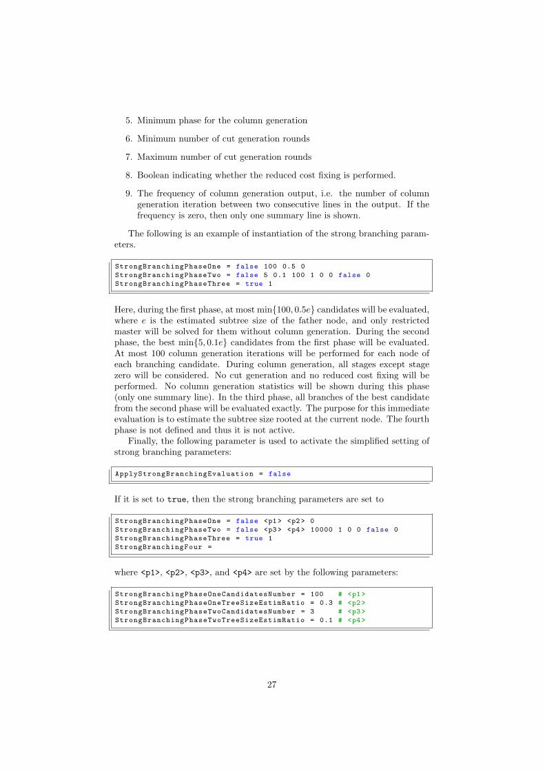
The following is an example of instantiation of the strong branching param-eters.

StrongBranchingPhaseOne = false 100 0.5 0

StrongBranchingPhaseTwo = false 5 0.1 100 1 0 0 false 0

StrongBranchingPhaseThree = true 1

Here, during the first phase, at most min{100, 0.5e} candidates will be evaluated,where e is the estimated subtree size of the father node, and only restrictedmaster will be solved for them without column generation. During the secondphase, the best min{5, 0.1e} candidates from the first phase will be evaluated.At most 100 column generation iterations will be performed for each node ofeach branching candidate. During column generation, all stages except stagezero will be considered. No cut generation and no reduced cost fixing will beperformed. No column generation statistics will be shown during this phase(only one summary line). In the third phase, all branches of the best candidatefrom the second phase will be evaluated exactly. The purpose for this immediateevaluation is to estimate the subtree size rooted at the current node. The fourthphase is not defined and thus it is not active.

Finally, the following parameter is used to activate the simplified setting ofstrong branching parameters:

ApplyStrongBranchingEvaluation = false

If it is set to true, then the strong branching parameters are set to

StrongBranchingPhaseOne = false <p1 > <p2> 0

StrongBranchingPhaseTwo = false <p3 > <p4> 10000 1 0 0 false 0

StrongBranchingPhaseThree = true 1

StrongBranchingFour =

where <p1>, <p2>, <p3>, and <p4> are set by the following parameters:

StrongBranchingPhaseOneCandidatesNumber = 100 # <p1 >

StrongBranchingPhaseOneTreeSizeEstimRatio = 0.3 # <p2>

StrongBranchingPhaseTwoCandidatesNumber = 3 # <p3>

StrongBranchingPhaseTwoTreeSizeEstimRatio = 0.1 # <p4>

27

4 BaPCod statistics

This section overviews the statistics which can be retrieved after solving themodel (see Section 2.1) for the methods to use.

4.1 Timers

The values of all timers are in ticks. To obtain the time in seconds, the valueshould be divided by 100.

bcTimeMain - overall solution time

bcTimeBaP - total branch-cut-and-price time (excludes formulations buildingtime and the final solution disaggregation)

bcTimeRootEval - solution time of the root (excluding primal heuristics andbranching)

bcTime1stLP - solution time of the first column generation convergence atthe root (before cut separation)

bcTimeColGen - total column generation time (all time to solve the masterproblem including generation of columns)

bcTimeMastMPsol - total time taken for solving the restricted master LPsby the LP solver

bcTimeCgSpOracle - total time taken for generation of columns (computingthe reduced cost of subproblem variables, solving the pricing problems,generating the columns from subproblem solutions, and adding columnsto the restricted master LP including computation of column coefficientsin the master constraints)

bcTimeSpUpdateProb - total time taken to compute the reduced cost ofsubproblem variables

bcTimeSpMPsol - total time taken to solve the pricing problems

bcTimeSetMast - total time to update the formulations of the master prob-lem and subproblems before solving a node

bcTimeSepFracSol - total branching time, i.e. generation of branching can-didates (evaluation of branching candidates in strong branching is notincluded)

bcTimeCutSeparation - total time for cut separation

bcTimeAddCutToMaster - total time for adding cuts to the restricted mas-ter LP (essentially computing coefficients of master variables and columnsin the cuts)

bcTimeRedCostFixAndEnum - total time for reduced cost fixing and enu-meration

bcTimeEnumMPsol - total time to solve enumerated MIPs

28

bcTimeSBphase1 - total time for evaluating branching candidates duringphase one of strong branching

bcTimeSBphase2 - total time for evaluating branching candidates duringphase two of strong branching

bcTimePrimalHeur - total time for running primal heuristics

Some times may “intersect”. For example, primal heuristic time includes apart of column generation time (in the case of diving heuristics). Evaluationtime for branching candidates also includes a part of column generation timeand a part of solving the restricted master LPs by the LP solver.

4.2 Records and counters

bcRecRootDb - the lower bound obtained at the root node (rounded up ifthe objective function is integer)

bcRecRootLpVal - the value of the master problem solution at the root node(not rounded even if the objective function is integer)

bcRecBestDb - final lower bound obtained by the branch-and-bound (roundedup if the objective function is integer)

bcRec1stLPDb - lower bound obtained by the column generation procedureat the root (before cut separation)

bcRecBestInc - best upper bound (value of the best feasible solution found)obtained by the branch-and-bound (the solution is optimal if this value isequal to bcRecBestDb)

bcCountCg - total number of iterations in the column generation procedure

bcCountCol - total number of generated columns (not all columns are neces-sarily added to the restricted master LP)

bcCountNodeProc - total number of processed nodes in the branch-and-bound tree

bcCountCutInMaster - total number of cuts added to the restricted masterLP

bcCountMastSol - total number of times the restricted master LP has beensolved by the LP solver

bcCountSpSol - total number of times the pricing problems have been solved

bcCountMastIpSol - total number of times the restricted master has beensolved as a MIP

29

5 BaPCod output

See Section 3.1 for the parameter to change the verbosity of the BaPCod out-put. It is possible to suppress all output except important warnings and errors.In the case the output is not suppressed, BaPCod will output the followinginformation.

At the beginning BaPCod prints its version:

~~~~~~~~~~~~~~~~~~~~~~~~~~~~~~~~~~~~~~~~~~~~~~~~~~~~~~~~~~~~~~~~~~~~~~~~~~~~

BaPCod v063, 2/09/2021, © Inria Bordeaux, France

~~~~~~~~~~~~~~~~~~~~~~~~~~~~~~~~~~~~~~~~~~~~~~~~~~~~~~~~~~~~~~~~~~~~~~~~~~~~

At the beginning of every branch-and-bound node, BaPCod outputs thefollowing information

************************************************************************************************ BaB tree node (N° 5, parent N° 3, depth 2)**** Local DB = 831.794, global bounds : [ 831.794 , 878.08 ], TIME = 1h22m49s40t = 496940**** 3 open nodes, 24679 columns (8375 active), 426 dyn. constrs. (199 active),

559 art. vars. (332 active)********************************************************************************************

The first line prints the index of the current node (indices are given in the orderof node creation), index of the father node, and the depth of the current node.The second line outputs the lower bound value of the current node, the globallower and upper bounds (valid for the model), and the current elapsed time.The third line outputs the current number of open branch-and-bound nodes (i.e.which were created but not yet pruned), and the aggregated information aboutthe restricted master problem. This information includes the total number ofcolumns in the memory (number of columns present in the current restrictedmaster LP), the total number of cuts and branching constraints in the memory(number of cuts and branching constraints present in the current restrictedmaster LP), the total number of artificial variables in the memory (the numberof artificial variables present in the current restricted master LP).

During the column generation procedure, BaPCod outputs the followinginformation

#<DWph=2> <it= 1> <et=4621.25> <Mt= 0.66> <Spt= 1.66> <nCl= 3> <al=0.50> <DB= 817.8515><Mlp= 830.2749> <PB=878.08035>

This information includes the current column generation phase (printed only ifthe number of phases is more than one), the current column generation iterationnumber, the current elapsed time, the time in seconds to solve the restrictedmaster LP in the current iteration, the total time in seconds taken for gener-ating columns in the current iteration (includes the time to solve the pricingproblems), the number of columns added to the restricted master LP in the cur-rent iteration, the current dual pricing smoothing stabilization parameter α (ifdual pricing smoothing stabilization is activated), the value of the Lagrangianlower bound at the current iteration, the value of the current restricted masterLP (upper bound on the solution value of the master problem), and the valueof the current best known feasible solution of the model (or the initial cut-offvalue given if not yet improved). If artificial variables are present in the currentsolution of the restricted master LP, then character # is printed in the beginningof the line.

30

In some cases, one line is printed per several column generation iterations.This can be recognized if the iteration numbers are not consecutive in twoconsecutive lines. In this case the time for solving the restricted master LP, thetime to generate columns, and the number of generated columns are aggregatedfor all iterations since the iteration of the previous line (or since the beginningof the column generation procedure).

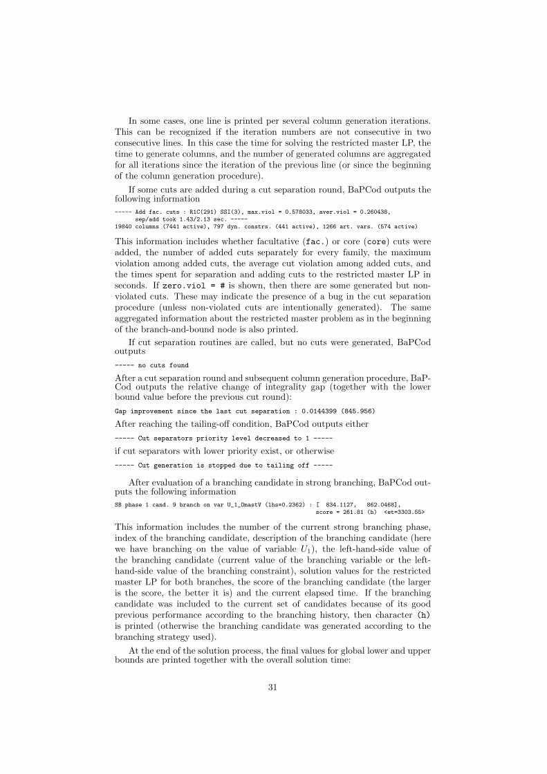
If some cuts are added during a cut separation round, BaPCod outputs thefollowing information

----- Add fac. cuts : R1C(291) SSI(3), max.viol = 0.578033, aver.viol = 0.260438,sep/add took 1.43/2.13 sec. -----

19840 columns (7441 active), 797 dyn. constrs. (441 active), 1266 art. vars. (574 active)

This information includes whether facultative (fac.) or core (core) cuts wereadded, the number of added cuts separately for every family, the maximumviolation among added cuts, the average cut violation among added cuts, andthe times spent for separation and adding cuts to the restricted master LP inseconds. If zero.viol = # is shown, then there are some generated but non-violated cuts. These may indicate the presence of a bug in the cut separationprocedure (unless non-violated cuts are intentionally generated). The sameaggregated information about the restricted master problem as in the beginningof the branch-and-bound node is also printed.

If cut separation routines are called, but no cuts were generated, BaPCodoutputs

----- no cuts found

After a cut separation round and subsequent column generation procedure, BaP-Cod outputs the relative change of integrality gap (together with the lowerbound value before the previous cut round):

Gap improvement since the last cut separation : 0.0144399 (845.956)

After reaching the tailing-off condition, BaPCod outputs either

----- Cut separators priority level decreased to 1 -----

if cut separators with lower priority exist, or otherwise

----- Cut generation is stopped due to tailing off -----

After evaluation of a branching candidate in strong branching, BaPCod out-puts the following information

SB phase 1 cand. 9 branch on var U_1_OmastV (lhs=0.2362) : [ 834.1127, 862.0468],score = 261.81 (h) <et=3303.55>

This information includes the number of the current strong branching phase,index of the branching candidate, description of the branching candidate (herewe have branching on the value of variable U1), the left-hand-side value ofthe branching candidate (current value of the branching variable or the left-hand-side value of the branching constraint), solution values for the restrictedmaster LP for both branches, the score of the branching candidate (the largeris the score, the better it is) and the current elapsed time. If the branchingcandidate was included to the current set of candidates because of its goodprevious performance according to the branching history, then character (h)

is printed (otherwise the branching candidate was generated according to thebranching strategy used).

At the end of the solution process, the final values for global lower and upperbounds are printed together with the overall solution time:

31

********************************************************************************************Search is finished, global bounds : [ 835.602 , 835.602 ], TIME = 1h48m56s75t = 653675********************************************************************************************

If values of global bounds are equal, then the best found solution is optimal.

6 VRPSolver extension

VRPSolver extension includes an implementation of the pricing functor whichallows the user to define the subproblems as resource constrained shortest pathproblems in graphs. The functor implements the bucket-graph based labelingalgorithm from paper [16] for solving the pricing problem, as well as the corre-sponding bucket arc elimination procedure (i.e. reduced cost fixing procedure),and the elementary route enumeration procedure [1]. VRPSolver extension alsoimplements cut separation functors for rounded capacity cuts [7] and limitedmemory rank-1 packing cuts [9], as well as packing set based Ryan-and-Fosterbranching, and branching over accumulated resource consumption [10]. Westrongly advise to read paper [12] before using VRPSolver extension. Please,cite this paper if your are using the VRPSolver extension. For the moment, theextension can be obtained in the compiled form (only for MacOS or Linux) byrequest from the corresponding author.

To use VRPSolver functors, one needs to include the corresponding headerfile:

#include "bcModelRCSPSolver.hpp"

6.1 VRPSolver pricing functor

To create such pricing functor one should use the constructor

BcRCSPFunctor(const BcFormulation & spForm );

Afterwards, this functor should be attached to the subproblem formulation asdescribed in Section 2.9 (BcRCSPFunctor inherits from BcSolverOracleFunctor).

The information about the resource-constrained path structure should begiven by defining a graph handler of type BcNetwork:

BcNetwork(BcFormulation & bcForm , NetAttrMask optionalAttrMask ,

int numElemSets , int numPackSets , int numCovSets );

Here bcForm is the subproblem to which we associate the graph. optionalAttrMaskshould always be equal to PathAttrMask. Other three arguments are the num-ber of elementarity sets, the number of packing sets, and the number of coveringsets. These sets are used to express elementarity, packing, and covering con-straints over the arcs and/or nodes of graphs (see [12]). The distance matrixfor elementarity sets can be passed using the following method of BcNetwork:

void setElemSetsDistanceMatrix(

const std::vector <std::vector <double >> & matrix );

32

Vertices and arcs of the graph can be defined using the following methodsof BcNetwork:

const BcVertex createVertex ();

const BcArc createArc(int tail , int head , double originalCost );

Here tail and head are the indices of the tail and head vertices of the arc,and originalCost is the “pure” cost of the arc. The coefficient of a columnrepresenting a path in a graph in the objective function is determined not onlyby the “pure” costs of its arcs, but also by objective function coefficients of sub-problem variables mapped to the arcs (see below how to map arcs to variables).An important notice here is that a special “cost” subproblem variable should becommunicated to the pricing functor if at least one arc has a non-zero “pure”cost:

void BcRCSPFunctor :: setPureCostBcVar(BcVar bcVar );

The value of this variable in the subproblem solution representing a path will beset to the total “pure” cost of arcs which form the path. To define the arc costone can alternatively map a variable to a subproblem variable (see below) anddefine a coefficient of this variable in the objective function (see Section 2.5).

The source and the sink of the graph can be defined using the followingmethods of BcNetwork:

void setPathSource(const BcVertex & vertex );

void setPathSink(const BcVertex & vertex );

Indices of vertices and arcs are always assigned in the order of creation ofvertices and arcs (starting from 0). These indices can be retrieved using methods

int BcVertex ::ref() const;

int BcArc::ref() const;

Vertices and arcs can be retrieved from their indices using the following methodsof the handler BcNetwork:

const BcVertex getVertex(int id) const;

const BcArc getVertex(int id) const;

One can add a vertex or an arc to an elementarity, packing, or covering setusing the following methods defined both for BcVertex and BcArc:

void setElementaritySet(int elemSetId );

void setPackingSet(int packSetId );

void setCoveringSet(int covSetId );

The set indices here should be not less than 0 and smaller than the correspondingnumber of elementarity, packing, or covering sets given in the constructor ofBcNetwork.

An arc can be mapped to a variable belonging to the same subproblem usingthe following methods of BcNetwork:

33

void addVarAssociation(const BcVar & newvar , const double coeff );

void arcVar(const BcVar & newvar );

The first method defines a mapping with an arbitrary coefficient, whereas thesecond method defines a standard mapping introduced in [12]. The standardmapping has coefficient 1.0. The coefficient of a column respresenting a path ina graph in a master constraint is determined by the scalar product of the vectorof coefficients of subproblem variables in this constraint and the sum of vectorsof mapping coefficients for the arcs which form the path.

A resource can added by defining the resource handler using the constructor

BcNetworkResource(const BcNetwork & bcNetwork , int id);

Here id is the index of the ressource. All resources should have different indices.By default, ressources are secondary and disposable (see [12] for the definition ofresource types). To define a main resource or a non-disposable resource, pleaseuse the following methods of BcNetworkResource:

void setAsMainResource ();

void setAsNonDisposableResource ();

Consumption of a resource for an arc can be defined using the following methodof BcNetworkResource:

void setArcConsumption(const BcArc & bcArc , double consumption );

Lower and upper bounds for the accumulated resource consumption can be de-fined on vertices and/or on arcs using the following method of BcNetworkResource:

void setArcConsumptionLB(const BcArc & bcArc , double consumptionLB );

void setArcConsumptionUB(const BcArc & bcArc , double consumptionUB );

void setVertexConsumptionLB(const BcVertex & bcVertex , double consLB );

void setVertexConsumptionUB(const BcVertex & bcVertex , double consUB );

At most 20 resources can be defined, among which at most two can be main.The main resource with the smallest index is used to determine the threshold forthe bi-directional labeling algorithm which solves the pricing problem (see [16]).

There is a possibility to define special resources for which the accumulatedresource consumption can be either 0 or 1 (i.e. binary resource). These resourcesare declared implicitly by defining consumption of such resources on arcs usingthe following method of BcArc:

void addBinaryResourceConsumption(int binaryResId , int consumption)

and by defining accumulated resource consumption bounds using the followingmethods of BcVertex:

void setSpecialResourceConsumptionLB(int binaryResId , int lowerBound );

void setSpecialResourceConsumptionUB(int binaryResId , int upperBound );

34

Here lowerBound and upperBound can take either value 0 or value 1. It makessense to only define non zero values for the (accumulated) resource consumption(bounds). The index (id) of a binary ressource can be between 0 and 511. Again,by default every binary resource is disposable. To declare a binary resource non-disposable, the following method of BcNetwork can be used:

void setSpecialResourceNonDisposable(const int binaryResId );

Besides solving a BaPCod model with RCSP functors in the standard way,one can also enumerate all feasible paths in directed graphs associated withsubproblems:

BcSolution BcModel :: enumerateAllColumns(int & nbEnumColumns );

The total number of enumerated columns is returned in nbEnumColumns, itis equal to -1 if enumeration did not succeed. The enumerated solutions arereturned in the solution chain, see Section 2.6 for details. This method shouldbe used for very small instances mainly for debugging and teaching purposes.

6.2 VRPSolver cut separation functors

The rounded capacity cuts [7] require an undirected graph G = (V ∪ {0}, E)with special “depot” node 0. There should be exactly one binary variable xeassociated with every edge e ∈ E. A positive demand dv should be associatedwith every non-depot node v ∈ V , and a positive capacity C should be defined.A rounded capacity cut is defined for a subset S ⊆ V of nodes. It states thatthere should be enough paths passing by set S to satisfy path capacity C:

∑e=(i,j): |{i,j}∩S|=1

xe ≥ 2 ·

⌈∑i∈S

di/C

⌉.

To add the functor for separation of rounded capacity cuts (the separationalgorithm follows paper [8]), on should use the constructor

BcCapacityCutConstrArray(const BcFormulation & formulation ,

const int & maxCapacity ,

const std::vector <int > & demands ,

const bool & isFacultative = true ,

const bool & equalityCase = true ,

const int & twoPathCutsResId = -1,

const double & rootPriorityLevel = 1.0,

const double & nonRootPriorityLevel = 1.0);

Here formulation is the master formulation handler, maxCapacity is the valuefor capacity C, demands is the vector d of demand values. Argument isFacultativedetermines whether cuts are facultative (separated only for fractional solutions)or core (separated also for integer solutions). Argument twoPathCutsResId

should be equal to -1. The remaining two arguments define the root and non-root priority level (see Section 2.8). This cut separator is introduced in [12].

The construction of undirected graph G = (V ∪ {0}, E) is based on alldirected graphs defined for subproblems of the BaPCod model. Vertices in

35

directed graphs defined for VRPSolver pricing functors are “projected” intovertices of graph G. The projection is defined based on packing sets(equalityCase=true) or on covering sets (equalityCase=false), and on vectorof demands. The first case (equalityCase=true) should be used when exactlyone vertex in every packing set should be visited exactly once (all other verticesin the set should not be visited). The second case (equalityCase=false) shouldbe used when at least on vertex in every packing set should be visited at leastonce (all other vertices in the set may or may not be visited). A vertex iin a directed VRPSolver graph is projected into vertex v ∈ V if i belongs topacking/covering set v and dv is positive. Otherwise, i is projected into depotvertex 0. An edge (v, v′) belongs to E if there exists an arc (i, j) in a directedgraph of VRPSolver such vertex pair {i, j} projects into vertex pair (v, v′). Inthis case, we say that arc (i, j) projects into edge (v, v′). A BaPCod variable isappropriate for an edge e ∈ E if it binary, mapped with coefficient one to everyarc (i′, j′) in directed graphs of VRPSolver which projects into edge e, and notmapped to any other arc with any coefficient.

Separation of rounded capacity cuts can be used only if

1. packing or covering sets (depending on argument equalityCase) are de-fined on vertices, i.e. no arc in any directed VRPSolver graph belongs topacking/covering set;

2. there exists exactly one appropriate BaPCod variable for every edge ofprojected graph G.

Appropriate variables are used to generate rounded capacity cuts. Note thatduring projection we loose information about arc direction. Nevertheless, thegenerated cuts remain valid. Moreover, separation of rounded capacity cuts ascore cuts is sufficient to replace the capacity resource in VRPSolver graphs if

• we are in the equality case (equalityCase=true);

• for every arc in VRPSolver directed graphs there exists an arc in theopposite direction;

• all vertices in VRPSolver directed graphs except the source and the sinkbelong to a packing set;

• all demands are positive and equal to all vertices belonging to the samepacking set;

• path capacity C is equal for all VRPSolver directed graphs.

In this case, declaration of the capacity resource may be skipped in VRPSolverdirected graphs. This may increase the performance when the capacity resourceis not tight (as for some Solomon instances of the Vehicle Routing Problem withTime Windows).

To add the functor for separation of limited-memory rank-1 cuts, on shoulduse the constructor

BcLimMemRankOneCutConstrArray(const BcFormulation & formulation ,

const double & rootPriorityLevel = 1.0,

const double & nonRootPriorityLevel = 1.0);

36

Here formulation is the master formulation handler, and the remaining twoarguments define that the root and non-root priority level (see Section 2.8).Limited-memory rank-1 cuts are introduced in [9]. VRPSolver uses the defini-tion of packing/covering sets in the model to separate rank-1 packing/coveringcuts (see [16]). VRPSolver pricing functor supports limited-memory rank-1 cuts.

6.3 VRPSolver branching functors

VRPSolver extension includes two functors for separating non-robust branchingconstraints (these constraints are supported in the pricing functor).

The first functor implementes separation of packing-set-based Ryan&Fosterbranching constraints. To add this functor, one should use the constructor

BcPackSetRyanFosterBranching(const BcFormulation & formulation ,

const double & priorityLevel = 1.0);

Here formulation is the master formulation handler, and priorityLevel isthe branching priority value (see Section 2.7). This functor searches branchingcandidates, each of which corresponds to a pair of packing sets (see [12] forthe definition of packing sets). A branching candidate generates two branchingconstraints. In the first one, the number of columns corresponding to pathswhich include arcs (or vertices) belonging to both packing sets is set be equalto one. In the second constraint, the number of such columns is set to be equalto zero.

There is also a possibility to define permanent packing-set-based Ryan&Fosterconstraints, using the method of BcNetwork:

void addPermanentRyanAndFosterConstraint(int firstPackSetId ,

int secondPackSetId ,

bool together );

This method adds the following constraint to the subproblems associated withthe graphs. In the case together=false, the path should include arcs (or ver-tices) belonging to at most one of packing sets firstPackSetId and secondPackSetId.In the case together=true, the path should include arcs (or vertices) belongingto non of these packing sets or to both of them.

The second functor implementes branching over accumulated resource con-sumption, introduced in [10]. To add this functor, one should use the constructor

BcElemSetResConsumptionBranching(const BcFormulation & formulation ,

const double & priorityLevel = 1.0);

Here formulation is the master formulation handler, and priorityLevel isthe branching priority value (see Section 2.7). This functor searches branch-ing candidates, each of which corresponds to a packing set p, threshold valueτ for accumulated consumption of resource with index 0. A branching can-didate generates two branching constraints. The first one forbids all columnscorresponding to paths in which an arc (or vertex) belonging to packing set pis visited when the accumulated consumption of resource 0 is less than τ . The

37

second one forbids all columns corresponding to paths in which an arc (or ver-tex) belonging to packing set p is visited when the accumulated consumption ofresource 0 is greater or equal to τ .

6.4 VRPSolver paramerization

First of all, the following parameters should be set when using VRPSolver ex-tension:

MaxNbOfStagesInColGenProcedure = 3

colGenSubProbSolMode = 3

The following additional parameters are defined for the VRPSolver exten-sion. Please consult [12] for more explanation about these parameters.

RCSPstopCutGenTimeThresholdInPricing = 10

RCSPhardTimeThresholdInPricing = 20

“Soft” and “hard” time thresholds in seconds for the labeling algorithm (τ soft

and τhard in the paper).

RCSPnumberOfBucketsPerVertex = 25

RCSPdynamicBucketSteps = 1

Parameters for calculation of step sizes for buckets (ψbuck and ψreduc in thepaper). Dynamic adjustment of bucket steps is on if RCSPdynamicBucketStepstakes value 1 and off if it takes values 0.

RCSPuseBidirectionalSearch = 2

Parameter to determine when the bi-directional labeling algorithm is used tosolve the pricing problem (φbidir in the paper): 0 — not used, 1 — always used,2 — used only during the exact column generation phase.

RCSPapplyReducedCostFixing = 1

Parameter to determine which bucket arc elimination (reduced cost fixing) pro-cedure is used (φelim in the paper): 0 — not used, 1 — standard bucket arcelimination procedure (follows [16]), 2 — light bucket arc elimination procedure(less strong, but faster), 3 — standard arc elimination procedure (similar to [5]),4 — light arc elimination procedure.

RCSPmaxNumOfColsPerExactIteration = 150

RCSPmaxNumOfColsPerIteration = 30

Maximum number of generated columns per column generation iteration andper subproblem with the RCSP pricing functor (γexact, γheur in the paper).The first parameter is for the exact column generation phase, and the secondparameter is for heuristic column generation phases.

38

RCSPmaxNumOfLabelsInEnumeration = 1000000

RCSPmaxNumOfEnumeratedSolutions = 1000000

RCSPmaxNumOfEnumSolutionsForMIP = 10000

RCSPmaxNumOfEnumSolsForEndOfNodeMIP = 0

The first two parameters are for the maximum number of labels and paths inthe elementary path enumeration procedure (ωlabels and ωroutes in the paper).The third parameter is for the maximum total number of enumerated paths totrigger the solving of enumerated MIP (ωMIP). The fourth parameter is for themaximum total number of enumerated path to trigger the solving of enumeratedMIP at the of a branch-and-bound node. The last parameter is active only ifits value is greater than the value of the third parameter.

RCSPinitNGneighbourhoodSize = 8

RCSPmaxNGneighbourhoodSize = 8

Initial and maximum size of ng-sets (ηinit and ηmax in the paper).

RCSPrankOneCutsMaxNumPerRound = 100

RCSPrankOneCutsMaxNumRows = 5

RCSPrankOneCutsMemoryType = 2

RCSPrankOneCutsLSnumIterations = 1000

Parameters for separation of limited-memory rank-1 cuts. First three ones cor-respond to parameters θnum, θrows, θmem in the paper. Possible values for thethird parameters are: 0 — automatic selection of node- or arc-memory (theroot node may be solved two times in this case), 1 — arc-memory is used, 2 —node-memory is used. The fourth parameters sets the number of iterations inthe local search heuristic to separate rank-1 cuts with four rows and more.

RCSPallowRoutesWithSameVerticesSet = true

Whether multiple paths which pass by the same set of vertices (in different order)can be generated in the same iteration of the column generation procedure.Setting this parameter to false may improve convergence (as more diversifiedset of paths is generated in every column generation iteration) but may slowdown the labelling algorithm as the additional check is necessary.

RCSPredCostFixingFalseGap = 0.0

If the value of this parameter is ≤ 1.0 that it has no effect. If its value is > 1.0then reduced cost fixing and enumeration are performed with the primal-dualgap is divided by this value, making the whole branch-cut-and-price algorithmheuristic. More about the false gap mechanism can be found in paper [14].

SafeDualBoundScaleFactor = -1

39

If this parameter is positive, it activates the calculation of the safe dual bound(parameter K in the paper). This may be important to avoid rounding errorswhen the objective function is to minimize the number of paths in the solution.Safe lower bounds for column generation were introduced in [4].

The following parameters are used to activate the primal heuristic which isbased on the elementary path enumeration with false gap. This heuristic wasproposed in [13] and was also used in [14].

RCSPmaxNumOfLabelsInHeurEnumeration = 0

MaxNumEnumSolsInRestrictedMasterIpHeur = 5000

If the first parameter is positive, then the elementary path enumeration is trig-gered at the end of a some branch-and-bound nodes (depends on parameterCallFrequencyOfRestrictedMasterIpHeur). The primal-dual gap is dividedby two each time the enumeration does not succeed for at least one subproblemassociated to the RCSP pricing functor. After succeeding enumeration, at mostMaxNumEnumSolsInRestrictedMasterIpHeur columns corresponding to pathswith the smallest reduced cost are added to the restricted master, and the latteris solved as a MIP. The restricted master heuristic parameters (see Section 3.5)also apply here.

6.5 VRPSolver output

To activate additional output of the VRPSolver extension, one needs to setparameter

DEFAULTPRINTLEVEL = 0

During the initialization of each RCSP pricing functor, the following infor-mation is shown:

RCSP solver info : symmetric case is detected for graph G_0!Bidirectional border value is initialised to 100RCSP solver info : number of forw. reachable buckets /

buck. strongly connected components is 3856( 97.5709% ) / 1931( 50.0778% )

The information whether the symmetric case is detected, the initial value forthe bi-directional threshold, and the initial number of reachable buckets andthe number of strongly connected components in the bucket graph (togetherwith the percentage from the total number of buckets). See paper [16] for anadditional explanation.

After each execution of the exact bucket-graph based labeling algorithm (seepaper [16]) to solve the RCSP pricing problem, some statistics are shown:

RCSP exact solver info for graph G_0 : TT = 0.092659, pt = 0.000274, dt = 0.079908,ct = 0.009966, ndl = 18’, bdl = 466’, odl = 15’, odf = 136’, bsi = 1’, cnt = 22’,bdch = 3616’, odch = 280’, lcp = 189’, #sols = 150

This statistics include:

• the index of the subproblem to which the directed graph is associated (G_0means index 0);

• TT: the total labelling time in seconds

40

• pt: preparation time in seconds (retrieving information about reducedcosts and non-robust cuts)

• dt: dynamic programming time in seconds (extension of labels and dom-inance checks)

• ct: concatenation time in seconds (in the bi-directional labeling)

• ndl : number of non-dominated labels in thousands

• bdl : number of labels dominated by labels in the same bucket, in thou-sands

• odl : number of labels dominated by labels in different buckets, in thou-sands

• odf : number of times the function which checks the dominance betweena label and all labels in a different bucket is called, in thousands

• bsi : number of times a bi-directional solution is inserted to the pool ofsolutions of the labeling algorithm, in thousands

• cnt : number of times a pair of forward and backward labels is tried forconcatenation, in thousands

• bdch : number of dominance checks between labels in the same bucket, inthousands

• odch : number of dominance checks between labels in different buckets,in thousands

• lcp : number of times a label is copied in the memory, in thousands

• #sols : number of solutions generated by the labeling algorithm

Every time the bucket arc elimination (reduced cost fixing) procedure islaunched, the following information is printed:

Reduced cost fixing for graph G_0... 40752 buck. arcs remain (79.1% from prev., 3.69% from max.)+ 41953 jump buck. arcs (3.8% from max.)TT = 2.81583, pt = 0.450316, dt = 1.11438, ct = 1.24473, ndl = 307’, bdl = 1252’, odl = 30’,odf = 1139’, lpcb = 1790’, cnt = 20528’, bdch = 40847’, odch = 28678’, lcp = 9921’

Labels distribution in buckets (bucket size) : largest - 507, top 0.1% - 472, top 0.5% - 376,top 2% - 277, top 10% - 114, top 50% - 9

Run forward enumeration with border = 100... succeeded! lpt = 1.53273, ndl = 95’, dl = 6’,lpcb = 912’, dch = 125’

Run enumeration concatenation with time limit 30.2322 sec.... succeeded!Sorting and storing enumerated solutions ... done!TT = 3.1909, pt = 0, dt = 1.53273, ct = 0.937832, ndl = 95’, bdl = 6’, lpcb = 912’, cnt = 11817’,bdch = 125’, odch = 0’, lcp = 0’

Enumeration succeeded!, number of elem. solutions is 103246Estimating inspection time... TT = 0.061083, performed by inspection with 103246 solutionsInspection time is low enough. Pricing will be done by inspection.Removed 5445 columns (not in the enumerated set) from the formulationRegenerated 2114 columns with the ’enumerated’ flag

First, the number of remaining bucket arcs after the reduced cost fixing proce-dure is printed for each direction together with the percentage from the numberof bucket arcs before the procedure and from the maximum possible number ofbucket arcs. Then the statistics of the reduced cost fixing procedure are printed

41

(similarly to the standard labelling algorithm). The time to determine whethera bucket arc can be eliminated or not is included in the concatenation time.Then, the labels distribution statistics is shown, i.e. the number of labels inthe largest bucket, and the minimum number of labels in 0.1%, 0.5%, 2%, 10%,and 50% of largest buckets. Afterwards, the elementary path enumeration pro-cedure is attempted, and its statistics are shown (which are again similar to tothe standard labelling statistics, except that there is no buckets). If enumer-ation procedure succeeds, the number of elementary solutions is shown. Thenthe inspection of these solutions (to calculate their reduced cost) is tried. If theinspection time is sufficiently low, the pricing problem passed to the “enumer-ated mode”. Then VRPSolver outputs the number of columns removed fromthe restricted master (because they do not correspond to any elementary so-lution in the enumerated set) and the number of columns regenerated (theircoefficients in master constrains may change as rank-1 cuts has full memory inthe enumerated mode).

When the elementary path enumeration procedure does not succeed, theratio between the final number of non-extended labels and the total number ofnon-dominated labels is shown:

Run forward enumeration with border = 100... not succeeded (ratio 0.513939)

The closer this ratio to zero, the closer is the enumeration procedure to besuccessful.

If the reduced cost fixing procedure is not called, then this information isshown:

Full reduced cost fixing is not called (gap ratio is 0.959188)Dynamic params and stats : aver.obdmd = 44.8224, aver.buck.num. = 51, nbR1C = 274

with avMem = 11.3285

This information contains the ratio of the current primal-dual gap in comparisonwith the primal-dual gap when the reduced cost fixing procedure was called thelast time (this ratio should be below the value of parameterReducedCostFixingThreshold to trigger the procedure). The information inthe next line contains the average value for the maximum depth when checkingdomination between labels in different buckets, the average number of bucketsper vertex, the number of active rank-1 cuts, and their average memory size.

When separating rank-1 cuts, the number of generated cuts for each numberof rows is shown together with the statistics for maximum and average violation:

3 Rank-1 1-rows pack. cuts added , max viol. = 0.0275816, aver. viol. = 0.0243375

88 Rank-1 3-rows pack. cuts added , max viol. = 0.104368, aver. viol. = 0.0337835

Building structures for heuristic rank-1 packing cut separation...done!

96 Rank-1 4-rows pack. cuts added , max viol. = 0.0791168, aver. viol. = 0.0348517

100 Rank-1 5-rows pack. cuts added , max viol. = 0.100438, aver. viol. = 0.0599266

7 Perspectives

BaPCod is a prototype (proof-of-concept) academic code which is not intendedfor an operational use in the industry. Bugs and numerical issues are expected.Thus, BaPCod is distributed for an academic use without any warranty. Theuser support is not guaranteed. Although critical issues and bugs will be ad-dressed by request, possibly with a delay. Corrections and extensions of this

42

user guide will also be done by request. No major developpement of BaPCodis planned in the future. On the other side, the work on the VRPSolver exten-sion will likely continue. We plan to extend modelling capabilities, implementadditional cut separation functors, and to improve the overall efficiency of VRP-Solver.

Acknowledgements

We appreciate financial support from Inria, Universite de Bordeaux, Institutede Mathematiques de Bordeaux, and CNRS (Centre Nationale de la RechercheScientifique, France).

We would like to thank many people who contributed to the design, im-plementation, and maintenance of BaPCod and VRPSolver extension: IssamTahiri, Laurent Facq, Boris Detienne, Aurelien Froger, Francois Clautiaux,Pierre Pesneau, Artur Pessoa, Eduardo Uchoa, Halil Sen, Jinil Han, CelineSaubatte, Franck Labat, Romain Leguay, Teobaldo Bulhoes, Guillaume Mar-quez, Eduardo Queiroga, Adeline Fonseca. The names are listed in no particularorder.

References

[1] Roberto Baldacci, Nicos Christofides, and Aristide Mingozzi. An exactalgorithm for the vehicle routing problem based on the set partitioningformulation with additional cuts. Mathematical Programming, 115:351–385, 2008.

[2] Hatem M.T. Ben Amor, Jacques Desrosiers, and Antonio Frangioni. On thechoice of explicit stabilizing terms in column generation. Discrete AppliedMathematics, 157(6):1167 – 1184, 2009.

[3] Jacques Desrosiers and Marco E. Lubbecke. Branch-price-and-cut algo-rithms. In Wiley Encyclopedia of Operations Research and ManagementScience. American Cancer Society, 2011.

[4] Stephan Held, William Cook, and Edward C. Sewell. Maximum-weightstable sets and safe lower bounds for graph coloring. Mathematical Pro-gramming Computation, 4(4):363–381, 2012.

[5] Stefan Irnich, Guy Desaulniers, Jacques Desrosiers, and Ahmed Hadjar.Path-reduced costs for eliminating arcs in routing and scheduling. IN-FORMS Journal on Computing, 22(2):297–313, 2010.

[6] O Kullmann. Handbook of Satisfiability, chapter Fundaments of branchingheuristics, pages 205–244. IOS Press, Amsterdam, 2009.

[7] G. Laporte and Y. Nobert. A branch and bound algorithm for the capaci-tated vehicle routing problem. Operations-Research-Spektrum, 5(2):77–85,Jun 1983.

[8] Jens Lysgaard, Adam N. Letchford, and Richard W. Eglese. A new branch-and-cut algorithm for the capacitated vehicle routing problem. Mathemat-ical Programming, 100(2):423–445, Jun 2004.

43

[9] Diego Pecin, Artur Pessoa, Marcus Poggi, and Eduardo Uchoa. Improvedbranch-cut-and-price for capacitated vehicle routing. Mathematical Pro-gramming Computation, 9(1):61–100, 2017.

[10] Artur Pessoa, Ruslan Sadykov, and Eduardo Uchoa. Solving bin packingproblems using vrpsolver models. Operations Research Forum, 2(2):20,2021.

[11] Artur Pessoa, Ruslan Sadykov, Eduardo Uchoa, and Francois Vander-beck. Automation and combination of linear-programming based stabiliza-tion techniques in column generation. INFORMS Journal on Computing,30(2):339–360, 2018.

[12] Artur Pessoa, Ruslan Sadykov, Eduardo Uchoa, and Francois Vanderbeck.A generic exact solver for vehicle routing and related problems. Mathemat-ical Programming, 183:483–523, 2020.

[13] Artur Pessoa, Eduardo Uchoa, and Marcus Poggi de Aragao. A robustbranch-cut-and-price algorithm for the heterogeneous fleet vehicle routingproblem. Networks, 54(4):167–177, 2009.

[14] Eduardo Queiroga, Ruslan Sadykov, and Eduardo Uchoa. A popmusicmatheuristic for the capacitated vehicle routing problem. Computers &Operations Research, page 105475, 2021.

[15] D. M. Ryan and B. A. Foster. An integer programming approach to schedul-ing. In A. Wren, editor, Computer Scheduling of Public Transport UrbanPassenger Vehicle and Crew Scheduling, pages 269 – 280. North-Holland,Amsterdam, 1981.

[16] Ruslan Sadykov, Eduardo Uchoa, and Artur Pessoa. A bucket graph–based labeling algorithm with application to vehicle routing. TransportationScience, 55(1):4–28, 2021.

[17] Ruslan Sadykov, Francois Vanderbeck, Artur Pessoa, Issam Tahiri, andEduardo Uchoa. Primal heuristics for branch-and-price: the assets of divingmethods. INFORMS Journal on Computing, 31(2):251–267, 2019.

[18] Francois Vanderbeck. Branching in branch-and-price: a generic scheme.Mathematical Programming, 130(2):249–294, 2011.

[19] Paul Wentges. Weighted dantzig–wolfe decomposition for linear mixed-integer programming. International Transactions in Operational Research,4(2):151–162, 1997.

44