BANK STRESS TESTS AND STOCK

MARKET PERFORMANCE

Aantal woorden/ Word count: 20400

Mathias Dendooven Stamnummer/ Student number: 01200086

Promotor/ Supervisor: Prof. dr. Rudi Vander Vennet

Masterproef voorgedragen tot het bekomen van de graad van:

Master’s Dissertation submitted to obtain the degree of:

Master of Science in Business Engineering

Academiejaar/ Academic year: 2016 - 2017

BANKS STRESS TESTS AND STOCK

MARKET PERFORMANCE

Aantal woorden/ Word count: 20400

Mathias Dendooven Stamnummer/ Student number: 01200086

Promotor/ Supervisor: Prof. dr. Rudi Vander Vennet

Masterproef voorgedragen tot het bekomen van de graad van:

Master’s Dissertation submitted to obtain the degree of:

Master of Science in Business Engineering

Academiejaar/ Academic year: 2016 - 2017

PERMISSION

I declare that the content of this Master’s Dissertation can be consulted and/or reproduced if the

sources are mentioned.

Name student: Mathias Dendooven

Signature:

Abstract

In this Master’s Dissertation, the impact of the 2014 EU-wide stress test on the stock market performance

of banks involved is considered. Stress tests have become an important tool in the supervisory process on

the banking system. It gave rise to a number of studies looking at the short-term impact on stock markets

and CDS markets. Here we assess the longer-term impact of the disclosure of the results on multiple

aspects of stock market performance, being the return, market risk and volatility. Following Fama and

French (1992), we use a cross-sectional regression model which allows us to investigate three research

questions: What long-run impact did the stress test have on the return, the market risk or the volatility of the

banks involved? Solving these questions will give an answer to the main research question, being: What, if

any, long-run impact did the 2014 EU-wide stress test have on the stock market performance of banks?

The results show us that there is indeed an influence stemming from the release of the stress test results

on the stock market performance of banks. However, a more precise answer to these questions differs

according to the banks under consideration. When looking at the full sample, there are some general

conclusions that can be made.

• Considering the return, markets seem, in general, to reward banks having a good stress test result.

This means that the capital ratio after stress testing positively influences bank returns. This

observation lasts in most cases only until one month after the release date of the stress test

results.

• For the market risk, most influence is no longer statistically relevant one month after the release of

the results. Overall, the better the results, the more market risk increases.

• Looking at the volatility, we find most influence occurring the first week after the release, where a

higher capital ratio after stress test increases the stability.

These findings show that there is indeed an influence of the stress test results on stock market

performance, most of which is to be found during the first month after the release date of the results.

I

Acknowledgements

I would like to thank prof. dr. Rudi Vander Vennet for providing me the opportunity to write this Master’s

Dissertation and giving useful advice. Furthermore, I would like to thank him for his inspiring classes in

which he brings over his passion for and expertise in the banking sector to the students.

I would also like to thank Thomas Present for giving useful advice and insights which have been of

important help.

Writing a Master’s Dissertation involves many days of work, but coming to the point at which one is able to

start working on a Master’s Dissertation many years. I would like to thank my parents for giving me the

opportunity to let me undertake this journey. In this regard, my father deserves special naming since he

gave me useful advice with regard to the setup of the data processing in this Master’s Dissertation.

Mathias Dendooven

Ghent, June 2017

II

Contents Acknowledgements .......................................................................................................................................... I

List of abbreviations........................................................................................................................................ III

List of tables and figures ................................................................................................................................ IV

1. Introduction .............................................................................................................................................. 1

2. Banking supervision ................................................................................................................................ 3

3. Stress testing ........................................................................................................................................... 7

3.1. General ............................................................................................................................................ 7

3.2. Stress test results ............................................................................................................................ 8

3.3. Stress test studies ......................................................................................................................... 10

4. Data ....................................................................................................................................................... 14

4.1. Data sources ................................................................................................................................. 14

4.2. Variables ........................................................................................................................................ 15

5. Return .................................................................................................................................................... 17

5.1. Methodology .................................................................................................................................. 17

5.2. Results ........................................................................................................................................... 18

5.3. Conclusion ..................................................................................................................................... 27

6. Market risk ............................................................................................................................................. 28

6.1. Methodology .................................................................................................................................. 28

6.2. Results ........................................................................................................................................... 28

6.3. Conclusion ..................................................................................................................................... 35

7. Volatility ................................................................................................................................................. 36

7.1. Methodology .................................................................................................................................. 36

7.2. Results ........................................................................................................................................... 36

7.3. Conclusion ..................................................................................................................................... 42

8. Limitations ............................................................................................................................................. 44

9. Conclusion ............................................................................................................................................. 45

9.1. What long-run impact did the stress test have on the return of the banks involved? ................... 45

9.2. What long-run impact did the stress test have on the market risk of the banks involved? ........... 46

9.3. What long-run impact did the stress test have on the stock market volatility of the banks

involved? .................................................................................................................................................... 46

9.4. Main research question: what, if any, long-run impact did the EU-wide 2014 stress test have on

the stock market performance of the banks involved? .............................................................................. 47

Bibliography ...................................................................................................................................................... I

III

List of abbreviations

AQR Asset Quality Review

BCBS Basel Committee on Banking Supervision

BIS Bank for International Settlements

CAPM Capital Asset Pricing Model

CDS Credit Default Swap

CEBS Committee of European Banking Supervisors

CET1 Common Equity Tier 1

df Degrees of Freedom

EBA European Banking Authority

EC European Commission

ECB European Central Bank

ESRB European Systemic Risk Board

EU European Union

JST Joint Supervisory Team

NCA National Competent Authority

SCAP Supervisory Capital Asset Program

SREP Supervisory Review and Evaluation Process

SSM Single Supervisory Mechanism

UMP Unconventional Monetary Policy

IV

List of tables and figures

Figure 1: Supervisory structure ..................................................................................................................... 5

Table 1: Stress test studies ........................................................................................................................... 10 Table 2: Summary statistics for independent variables................................................................................. 16 Table 3: Summary statistics for weekly returns of MSCI Europe and all banks (average values) ............... 16 Table 4: Regression results overall effects-equation 1 ................................................................................. 19 Table 5: Regression results overall effects-equation 2 ................................................................................. 19 Table 6: Regression results non-vulnerable countries-equation 1 ................................................................ 20 Table 7: Regression results non-vulnerable countries-equation 2 ................................................................ 21 Table 8: Regression results vulnerable countries-equation 1 ....................................................................... 21 Table 9: Qualitative analysis of grouping banks according to β (average values) ........................................ 22 Table 10: Qualitative analysis of grouping banks according to stress test result (average values) ............. 22 Table 11: Qualitative analysis of grouping banks according to β and stress test result (average values) ... 23 Table 12: Regression results grouping according to β – equation 1 (26/10-28/11) ...................................... 24 Table 13: Regression results grouping according to β – equation 1 (26/10-26/12) ...................................... 24 Table 14: Regression results grouping according to β – equation 2 (26/10-21/11) ...................................... 25 Table 15: Regression results grouping according to β – equation 2 (26/10-26/12) ...................................... 25 Table 16: Regression results grouping according to post-stress test result-equation 2 (26/10-21/11) ........ 26 Table 17: Regression results grouping according to post-stress test result-equation 2 (26/10-26/12) ........ 26 Table 18: Regression results overall effects – equation 1 ............................................................................ 29 Table 19: Regression results overall effects – equation 2 ............................................................................ 30 Table 20: Regression results non-vulnerable countries – equation 1 ........................................................... 31 Table 21: Regression results non-vulnerable countries – equation 2 ........................................................... 31 Table 22: Regression results vulnerable countries – equation 1 .................................................................. 32 Table 23: Regression results vulnerable countries – equation 2 .................................................................. 32 Table 24: Regression results grouping according to post-stress test result-equation 1 (26/10-31/10) ........ 33 Table 25: Regression results grouping according to post-stress test result-equation 1 (26/10-21/11) ........ 33 Table 26: Regression results grouping according to post-stress test result-equation 1 (26/10-26/12) ........ 33 Table 27: Regression results grouping according to post-stress test result-equation 2 (26/10-31/10) ........ 34 Table 28: Regression results grouping according to post-stress test result-equation 2 (26/10-21/11) ........ 34 Table 29: Regression results grouping according to post-stress test result-equation 2 (26/10-26/12) ........ 34 Table 30: Regression results overall effects – equation 1 ............................................................................ 37 Table 31: Regression results vulnerable countries – equation 1 .................................................................. 37 Table 32: Regression results vulnerable countries – equation 2 .................................................................. 38 Table 33: Regression results non-vulnerable countries – equation 1 ........................................................... 38 Table 34: Regression results non-vulnerable countries – equation 2 ........................................................... 38 Table 35: Regression results grouping according to β – equation 1 (26/10-31/10) ...................................... 39 Table 36: Regression results grouping according to β – equation 1 (26/10-21/11) ...................................... 39 Table 37: Regression results grouping according to β – equation 1 (26/10-26/12) ...................................... 40 Table 38: Regression results grouping according to β – equation 2 (26/10-31/10) ...................................... 40 Table 39: Regression results grouping according to β – equation 2 (26/10/-21/11) ..................................... 40 Table 40: Regression results grouping according to β – equation 2 (26/10-26/12) ...................................... 41 Table 41: Regression results grouping according to post-stress test result–equation 1 (26/10-31/10) ........ 41 Table 42: Regression results grouping according to post-stress test result–equation 1 (26/10-21/11) ........ 42 Table 43: Regression results grouping according to post-stress test result–equation 1 (26/10/-26/12) ....... 42

1

1. Introduction

Since 2009, when the banking system was shaken up and its health being heavily questioned, bank

supervisors added a new tool to their supervisory toolbox: stress tests. In an environment of uncertainty,

investors were reluctant to invest in the banking industry, not knowing whether banks were able to survive

potential additional shocks in the aftermath of what had happened in the years before. Not only investors,

but also supervisors were concerned with this question. As Schuermann (2014) pointed out: “It is perhaps

the most basic of risk-based questions to want to know the resilience of an exposure to deteriorating

conditions.” (Schuermann, 2014, p.721). In order to increase transparency in banks’ balance sheets and

in an effort to increase bank health, stress tests were introduced as a new (and by now standard) tool of

the bank supervisor. Stress testing in itself is not a new concept (as we will point out later), however the

extent and size of the recent stress tests is quite different: macroeconomic adverse scenarios, complete

entities being tested, and an increased regulatory attention. By now, a number of stress tests are

conducted since 2009. The latest one is conducted in the U.S. in 2017 (the results are to be disclosed by

the end of June) and in the EU in 2016 (with the next one planned in 2018). The stress tests gave rise to

a number of new academic studies, dealing with the quality of the tests, the benefits and costs, and also

considering the effect these exercises have on banks’ stock market performance. Examples of the latter

are Alves, Mendes and da Silva (2015), Gerhardt and Vander Vennet (2017) or Sahin and de Haan

(2016) who describe the impact of different stress tests on stock prices and CDS spreads. These studies

have in common that they use an event study methodology to formulate conclusions, and consider a brief

time period after the results (or official intermediate announcements) are released.

However, one approach that is not considered in literature is the effect of these stress tests on stock

market performance over an extended period of time. This Master’s Dissertation aims at touching upon

this approach and considers the impact of the EU-wide stress test conducted in 2014 on bank stock

market performance over an extended period of time. The main research question that we try to answer is

therefore: what, if any, long-run impact did the EU-wide 2014 stress test have on the stock market

performance of the banks involved? The term long-run is initially determined as starting at the release

date of the stress test results and ending at the release date of the 2016 EU-wide stress test results.

However, this will be subdivided into several sub periods in order to have a better view on the evolution of

the impact. The smallest period we consider is one week after the release of the results, which is

arguably long-run. Nevertheless, this period is towards the upper limit of event study periods and

therefore also considered as long-run. When talking about stock market performance, not only return, but

also volatility is an important aspect. Next to general volatility, also volatility compared to the market (the

market risk) is of interest for investors and is also considered. Therefore, the main research question can

be subdivided into three different questions: (1) What long-run impact did the stress test have on the

return of the banks involved?, (2) What long-run impact did the stress test have on the market risk of the

banks involved?, and (3) What long-run impact did the stress test have on the stock market volatility of

the banks involved?

2

The next section gives an introductory overview of several supervisory entities and their responsibilities.

Section 3 focuses on what exactly a stress test is, and how it is conducted at the several financial

institutions. Results of several EU-wide stress tests are discussed as well, followed by an overview of

studies that describe the impact and best practices of stress tests. In section 4 the data used in this study

are discussed, as well as the criteria to which these data had to comply. We also sum up the variables

used in the subsequent models.

Section 5 discusses the first of three research questions that are derived from the main research

question, namely the impact of the 2014 EU-wide stress test on the return of the banks involved.

Subsequently the second research question is discussed in section 6, which considers the impact on the

market risk. The answer to the third and final research question is given in section 7, that discusses the

impact on volatility. The limitations to the research conducted are considered in section 8, while a general

conclusion that includes the answer to the main research question is given in section 9.

3

2. Banking supervision

Banks are subject to a number of regulations stemming from different regulatory authorities. One

institution that houses an international standard setting body is the Bank for International Settlements

(BIS). The BIS promotes international cooperation among other supervisory bodies from across the world,

through on the one hand organizing periodical meetings and on the other hand by the Basel Process

(BIS, s.d.-b). The Basel Process is an overarching term that refers to the assembly of groups that are

engaged in standard setting processes. Among those is the Basel Committee on Banking Supervision

(BCBS), whose task it is to set global standards for prudential regulation of banks (BIS, s.d.-a). It is the

BCBS who developed and oversees the implementation of Basel III, the new regulatory framework which

came into place as of 2011 and is gradually phased in until 2019, as a reaction to the financial crisis. One

of the most important aspects of this new regulation is the increased capital requirement, which serves as

a buffer to capture unexpected losses.

The attention paid to capital requirements comes back in the supervisory actions taken on a European

level as well1. In Europe, and more specifically the European Union (EU), we have to distinguish between

euro area and non-euro area countries concerning the supervisory authorities. For both types of

countries, the European Banking Authority (EBA) is the authority that sets prudential regulations and

organizes bank supervision. The EBA is an organization of the EU which is founded in 2011 and replaces

the former Committee of European Banking Supervisors (CEBS). Its objectives are “to maintain financial

stability in the EU and to safeguard the integrity, efficiency and orderly functioning of the banking sector”

(EBA, s.d.). The reason for founding such an institution is to promote a more integrated approach to

banking supervision across the EU. Therefore, one of the main purposes of the EBA is to develop one

rulebook that is applicable to all banks in the EU, and as such to contribute to the creation of a single

market in the banking sector (EBA, 2016c).

Next to a single rulebook, developing regulatory standards is another activity of the EBA. These

regulatory standards, bundled in a so-called single supervisory handbook (EBA, 2016c), ensure that

supervisors across EU member states use the same methodologies to evaluate banks. As such they

ensure a consistent supervision across the EU, termed supervisory convergence. This contributes to a

greater financial stability within the EU (EBA, 2016c).

Another task of the EBA is risk assessment. The EBA conducts both one-time and returning risk related

research. For example, the Risk Assessment Reports provide an overview of the current risks presented

in the financial sector and acts as an early warning signal. It is also in this regard that the EBA provides

the standard methodology for the stress tests, which it also coordinates2. The resulting data of these risk

assessments can be consulted on the website of the EBA3. This gives a high level of transparency and

therefore can help reduce market uncertainties, resulting again in more financial stability.

1 Although this is also the case for other parts of the world, we focus here on the European Union level. 2 The next section will go into more detail with regard to the stress tests. 3 www.eba.europa.eu

4

Another institution of interest in this section is the European Central Bank (ECB). The role of the ECB is

somewhat unusual. Next to being a central bank, it is also the bank supervisor for all euro area countries.

In its role as a central bank, the ECB cooperates with the central banks of all 19 countries that constitute

the euro area to form the Eurosystem. The ECB Governing Council is the main decision-making body

within the Eurosystem. The ECB takes on the traditional tasks of a central bank together with the national

central banks. With regard to monetary policy, the Eurosystem is tasked to maintain price stability across

all 19 EU countries having the euro as their home currency. Its main tool to achieve this price stability is

the setting of key interest rates. The Governing Council of the ECB, who is the monetary policy maker,

recently had to make use of not only the interest rate setting, but also of a number of unconventional

monetary policy measures (UMP) during the course of the financial crisis, sovereign crisis and thereafter.

For an overview of these measures and the effect they had we refer to the literature, for example Pill and

Reichlin (2014), or (Pattipeilohy, Van Den End, Tabbae, Frost, & De Haan, 2013). More recent work

which also gives an evaluation of the Asset Purchase Programme is done by for example Andrade,

Breckenfelder, De Fiore, Karadi and Tristani (2016).

Next to being a central bank, the ECB assumes another role as well. As of 4/11/2014, the Single

Supervisory Mechanism (SSM) came into place. This implies that the ECB is the single responsible

authority for bank supervision in the Eurozone4. Nevertheless, only the most significant banks5 fall under

direct supervision of the ECB, while the others remain under direct supervision of national supervisors.

Until November 2014, the supervision of all banks was arranged on a national level. However, the

creation of the SSM was important given the fact that banks operated already on a European level and

were highly interrelated. Therefore, the supervision of these banks should be organized on European

level as well in order to be effective and to take into consideration the interests of the Eurozone as a

whole (see, for example, Gros (2012)). Quaglia (2013) also mentions the improper regulation of some

financial institutions, the costs related to the bail-out of cross-border financial institutions and the financial

crisis as reasons to establish a macro-prudential oversight of the financial sector on EU level.

As mentioned, the SSM implies that the ECB is the final responsible for bank supervision in the Eurozone

and exercises this supervision in cooperation with national competent authorities (NCA). For each

significant bank, a Joint Supervisory Team (JST) is composed. In such a team, ECB experts work

together with experts from the relevant NCAs. This team also has a sub-coordinator (from an NCA) who

is responsible for specific domains or specific geographic areas and supports the coordinator of the JST,

which forms the link with the remainder of the ECB supervisory structure (ECB, 2017).

In its role as a supervisor, the ECB acts on Pillar 2 from the Basel III regulation, namely Supervisory

Review and Evaluation Process (SREP). This Pillar 2 describes some supervisory tasks and tools that

allow supervisors to evaluate banks based on their safety and compliance with prudential regulation.

SREP gives supervisors more authority to act upon the specific risk profile of individual banks, with as

final goal to increase the safety of the banking system. The procedure to determine such a risk profile is

based on four key domains, namely the bank’s business model, governance and risk management,

4 Also non-euro area countries can join the SSM, with a ‘close cooperation’ system as determined by the ECB

Governing Council (2014b). 5 The significance of a bank is determined using a number of criteria, among which size and cross-border activities.

5

capital and also liquidity. Based on these focus points, the supervisor comes up with an overall

assessment of each individual bank. This assessment is a sort of score with an overview of the most

important conclusions and is used to determine some bank-specific requirements in addition to the

baseline requirements formulated in Pillar 1. These can be quantitative requirements such as additional

capital that needs to be hold, or qualitative ones such as restrictions on business activities. Important

tools for evaluation are stress tests, which will be discussed in the next section. Next to the guidelines

provided by the BCBS, the ECB is also subject to the technical standards as developed by the EBA

(ECB, 2014d).

In addition to this micro prudential oversight, the ECB is also responsible for macro prudential oversight.

In this case it ensures the stability of the financial system as a whole rather than for individual banks,

which means that the ECB monitors the build-up of systemic risks and vulnerabilities. It performs this task

again in collaboration with NCAs and with the European Systemic Risk Board (ESRB) (ECB, 2014d). The

fact that the ECB is a supranational institution gives it the advantage of being in a very suitable position to

identify potential systemic risks across the Eurozone, rather than on a national level. With respect to this

macro prudential oversight, the ECB also determines the countercyclical capital buffer to be held by

banks (as described in Pillar 1 of Basel III). The figure below summarizes the supervisory structure as

described above, focusing on the EU.

Figure 1: Supervisory structure

The ECB, as mentioned before, assumes two roles: on the one hand, it is the centre of the Eurosystem,

which is the role of central banker; on the other hand, it is the centre of Banking Supervision, which is the

role of supervisor. The problem with assuming both roles is that they can be conflicting sometimes.

Monetary policy measures taken by the central bank can have negative implications for banks, going

6

against the aim of the supervisor of ensuring a stable banking system. Vice versa, if the supervisor

imposes certain measures on banks, this can have an impact on the price stability.

In order to ensure an independent functioning of both the ECB-central banker and the ECB-supervisor, a

Chinese wall is built between both. This becomes visible in the decision-making processes and the

organizational structure of the ECB. The latter is made separately for the central bank and the supervisor,

each having their own set of directorates and central body. This central body for the central bank is the

Governing Council, while for the supervisor this is the Supervisory Board. Decisions made by the

supervisory division follow the non-objection procedure (ECB, 2014d). According to this procedure, the

Supervisory Board prepares draft decisions (regarding bank supervision) and submits them to the

Governing Council. The latter then has ten working days to either adopt or object the draft decision. If no

reaction is given within this period, the decision is automatically adopted. Note that the Council cannot

change decisions. If it objects to the draft decision, the draft is sent back to the Supervisory Board and a

Mediation Panel resolves the conflicting views.

7

3. Stress testing

3.1. General

Stress testing is a test used in different settings, among which the banking sector. The general purpose is

to see how a system (in this case a bank) reacts to adverse circumstances. Specifically in the banking

sector, stress tests are used by regulators in order to determine the resilience of banks to adverse

macroeconomic developments and to impose additional capital measures to strengthen this resilience if

needed. These tests were not new to the banking sector in 2014. The first notions of it can be found in the

1995 Market Risk Amendment to the Basel 1 accord, established in 1988. However, the formal stress

testing as known today is more recent, of which the US bank stress test (Supervisory Capital Assessment

Program – SCAP) in 2009 and the EU stress test performed by the predecessor of the EBA, the CEBS,

are the first major examples (Schuermann, 2014).

When focusing again on the EU level, the EBA (and before the EBA, the CEBS) is the institution

performing EU-wide stress testing exercises, in collaboration with NCAs. More specifically, the EBA

provides, in its role as a standard setting institution, a consistent methodology, common risk factors and

uniform threshold level (which is the capital ratio (as defined further) banks need to obtain after stress

testing). The NCAs are the ones who are overseeing the correct application of these risk factors on each

individual bank and the correctness of the results per bank. Three stress tests were conducted during the

period 2009-2011. The stress test performed in 2014 was somewhat different: in the advent of the SSM,

the ECB wanted a financial health check held at the Eurozone banks in order to prevent its supervisory

activities being impeded by legacy issues. This financial health check was composed out of two parts: an

Asset Quality Review (AQR)6 and a stress test. For the 2014 stress test, the coordination became a

shared responsibility between the EBA and the ECB, at least for countries participating in the SSM (EBA,

2014b).

An important decision to be taken by the regulator is what the adverse macroeconomic scenario should

look like and what the requirements are for banks to pass the test. Concerning the latter, there are

several requirements set, but the main requirement is maintaining a sufficiently high capital ratio, defined

as eligible capital over (risk weighted) assets, after running the adverse scenario on the bank’s balance

sheet. Several macroeconomic factors are taken into account when developing a stress test.

Schuermann (2014) points out that when developing the scenario, consistency is important as well. He

illustrates this with exchange rates: one cannot let all exchange rates depreciate at once, some have to

appreciate if others depreciate.

The adverse scenario used in the EU-wide stress tests is developed each time by the ESRB, who takes

the prevailing systemic risks at the time of stress testing as a basis (ESRB, 2014). In 2014, the most

important systemic risks as defined by the ESRB General Board were (1) an increase in global bond

yields, (2) worsening of credit quality in countries with a weak banking sector, (3) stalling policy reforms

6 The purpose of an AQR is to have a good overview of bank exposures and the correctness of their valuation (ECB,

2014e).

8

and (4) the absence of important bank balance sheet repairs. These four systemic risks give rise to

several important shocks being simulated. For example, the 2014 adverse scenario lets the government

bond yield of the US rise with 100 basis points, gradually increasing until 250 basis points and eventually

level off to 150 basis points above the baseline scenario (see further). This causes the EU long term

interest rates to increase, as well as the spreads between EU sovereign bond yields (ESRB, 2014). Other

examples of shocks are currency shocks for specific currencies (based on past crisis experiences)

shocks in swap rates and a significant downturn in real estate markets (ESRB, 2014).

Next to an adverse scenario, the stress test contains a baseline scenario as well. This is a scenario

provided by the European Commission (EC), based on forecasts of the real economic situation. For the

2014 stress test, the baseline scenario was based upon the winter 2014 European Economic Forecast

from the Directorate General for Economic and Financial Affairs of the EC (European Commission, 2014).

This baseline scenario again describes the evolution of a number of key variables such as GDP growth

and house prices (European Commission, 2014).

3.2. Stress test results

As mentioned, the NCAs and the ECB are responsible for the quality of the stress test results for each

bank. These results are then collected by the EBA, who acts as “a data hub for the extensive

transparency of the results of the common exercise“ (EBA, 2014b). This transparency can be found back

in the fact that the EBA makes the results publicly available, not only in the form of a report but also in the

form of data sets, releasing a large amount of data that can be interpreted according to the vision of the

reader of these results. By increasing the transparency, the EBA hopes to increase market discipline of

banks as well as to underpin the credibility of the exercise (given the fact that analysts can access the

data and interpret them themselves as well). Also in previous stress tests, the EBA (or the CEBS) acted

as data hub for the results. We will now briefly consider the results of these tests. For a full review of the

results of the different stress tests, we refer to the official reports made by the EBA7.

In 2009, the CEBS stress test was conducted on 22 major European cross-border banking groups, with

the aim to increase the information among policy makers with regard to the resilience of the financial

system on European level (CEBS, 2009). The exercise consisted of both a baseline and adverse

scenario. The threshold for banks was to fulfil the Basel minimum requirement of 4% capital ratio in the

baseline scenario and to consider the impact of an adverse scenario for a period of 2 years. Capital ratio

can be defined as the ratio of eligible capital over (risk weighted) assets. As a result, the aggregate

capital ratio was 9% in the baseline scenario and a one percentage point decrease when exposed to the

adverse scenario. This is a rather positive result, but as mentioned by the CEBS this is also due to the

support provided by the public sector in the form of capital injections and asset guarantees.

The results of 2010 are again used to assess the resilience of the banking sector to an adverse

macroeconomic environment over a 2-year period. 91 banks were tested for their capital adequacy in a

baseline and adverse scenario. Of these 91 banks, 7 did not pass the hurdle rate of 6% tier 1 capital ratio

in the adverse scenario as imposed by the CEBS. The aggregate result was a 9.2% tier 1 capital ratio

after stress testing. However, as was the case in 2009, in this capital ratio we have to take into account

7 These reports can be retrieved from: http://www.eba.europa.eu/risk-analysis-and-data/eu-wide-stress-testing

9

the effect of the government support which accounted for approximately 1.2% of the aggregate result

(CEBS, 2010). The results of this stress test were weakened off by later events: as noted by Schuermann

(2014), a subsequent stress test of Irish banks resulted in a capital shortfall for several banks that passed

the CEBS stress test.

90 banks were tested in 2011, the first year in which the EBA replaced the CEBS. Again, the resilience of

banks was tested over a 2-year period and a hurdle rate with regard to the capital ratio after stress testing

was set. This hurdle rate was defined as 5% core tier 1 capital ratio (EBA, 2011). This threshold is

defined differently from the ones used by the CEBS in that core tier 1 is a more narrow definition of capital

as is tier 1, hence this hurdle rate is more strict. Another difference with earlier stress tests is the amount

of transparency: for the first time, the data behind the results was released and available to the public.

These results indicated that eight banks did not pass the 5% core tier 1 capital ratio threshold. 16 other

banks had a ratio between 5% and 6% (EBA, 2011). Failing the stress test had implications for the bank:

the EBA stated that all banks falling below the threshold should come up with a plan to restore their

capital positions, to be presented to their competent authorities by October 2011. The actual restoring to

at least the threshold level should be finished by end 2011. In addition to this, the EBA recommended

NCAs to request banks with capital ratios close to the hurdle rate to take action as well.

In 2014, the stress test conducted by the EBA was the biggest so far (including 123 banks), ran over 3

years and provided a high level of transparency to the public. Up to 12000 data points per bank were

released, available in spreadsheet format which, as mentioned before, allows analysts to test their own

assumptions. The aim of the stress test is again to determine the resilience of the banks against adverse

macroeconomic developments. Additionally the EBA mentions the completion of the repair of the EU

banking sector and the increase of the confidence in these banks (EBA, 2014a), which is supported by

the applied transparency.

The 2014 stress test is different from previous exercises in that it is a comprehensive assessment. This

means that before the actual stress test is conducted, an AQR took place. This assessment of the quality

of the valuation of bank assets lead to an adjustment of €47.5 billion to these assets8 (ECB, 2014a). After

these adjustments, banks were required to have 8.0% common equity tier 1 (CET1) ratio. This is also the

ratio that was required under the baseline scenario. In the adverse scenario, the hurdle rate was set at

5.5% CET1 ratio. Banks started the test with an average of 11.1% CET1 ratio (after adjustments based

on AQR), which decreased to 8.5% after stress, where the main causes of the losses are credit losses

and an increase in risk weighted assets. 24 banks did not pass the hurdle rate. However, when taking into

account recapitalisations that occurred in 2014 this number reduces to 14 (EBA, 2014c). Supervisory

authorities came up with a strict timeline for those banks that have shortfalls. The banks that had a

shortfall identified in the AQR or in the baseline scenario had to cover this by April 2015, those with a

shortfall identified in the adverse scenario by July 2015.

The latest EBA stress test was conducted in 2016. This exercise covered 53 banks, of which 39 that fall

under the scope of the SSM. Approximately 70% of the EU banking sector is covered and includes again

a baseline and an adverse scenario, running over a 3-year period starting from end 2015 until end 2018

(EBA, 2016a). With the aim of further increasing market discipline, the transparency of the exercise

8 The total asset value of all participating banks was €22.0 trillion (ECB, 2014a)

10

increased even further compared to the 2014 stress test, with more than 16000 data points released per

bank (EBA, 2015). An interesting fact is that no capital threshold is defined. The aim of the test, next to

the comparison and assessment of bank resilience, is to provide input to the 2016 SREP, where

appropriate decisions can be made on a bank-by-bank level regarding the capital requirements. This

means, to use the same expression as the EBA, that the focus remains on the repair of the EU banking

sector (EBA, 2016b). As starting capital ratio end 2015, an average CET1 ratio of 13.2% was found. After

stress testing, this ratio decreased 380 basis points to an average of 9.4% end 2018. The main drivers of

the decrease in capital ratio are credit losses, operational risk and market risk (EBA, 2016b).

3.3. Stress test studies

In the literature, there are several studies to be found that deal with different aspects of stress tests.

Some consider relevance, while others consider the market reaction to the outcome of the tests. The

following table provides an overview of studies that are discussed below.

Study Subject

Acharya, Engle and Pierret (2014)

Comparison of the capital shortfall in regulatory

stress test to a benchmark methodology and

assessment of risk measures used

Alves, Mendes and da Silva (2015)

Research whether the disclosure of two EBA

stress tests conducted during the sovereign debt

crisis (2010 and 2011) impacted the stock

markets and CDS markets

Camara, Pessarossi and Phillipon (2016) Evaluation of the quality of stress tests

Candelon and Sy (2015) Comparing the market reaction on U.S. and EU

stress tests performed between 2009 and 2013

Fritz-Morgenthal, Hellmuth and Packham (2016)

Research on the relation between risk culture and

stress indicators, and which of the risk indicators

best explains the 2014 stress test results

Gerhardt and Vander Vennet (2017)

Research how not only the end result, but six

different official announcements during the 2011

EBA stress test affected banks’ stock returns

Goldstein and Sapra (2014) The costs and benefits related to the extent of

disclosure of stress test results

Petrella and Resti (2013) Whether and how the 2011 stress test conducted

by the EBA affected bank stock prices

Sahin and de Haan (2016)

The impact of the 2014 comprehensive

assessment on banks’ stock prices and CDS

spreads

Table 1: Stress test studies

11

Acharya, Engle and Pierret (2014) compare the stress test methods used in the 2009 U.S. stress test and

the 2011 EU-wide stress test with another method to assess bank financial performance under stress,

namely the “V-lab stress test” (Acharya et al., 2014). This method uses a measure called SRISK, which

tries to capture the amount of capital that would need to be raised to return to a target capital ratio during

an economic crisis. Their results show that the V-lab stress test imposes larger recapitalization

requirements on banks. Furthermore, the V-lab risk weight (defined as risk-weighted assets to total

assets) and the average regulatory risk weight is uncorrelated, where the authors find that the average

risk weight of European banks is not related to their actual risk and that, using these weights, an incentive

is created for banks to actually be less diversified. They indicate that the regulatory stress test would be

more effective if, in addition to the capital ratio based on risk-weighted assets, a capital ratio based on

unweighted assets (the leverage ratio) and market-based risk measures were added.

The study of Alves, Mendes and da Silva (2015) addresses several questions in order to assess whether

the stress tests conducted by the EBA in 2010 and 2011 brought up new information that was processed

into Credit Default Swap (CDS) prices and stock prices of banks, hereby using the event study

methodology. They conclude that the 2010 stress test positively influenced stock prices. The stocks of

banks that underwent the test (and especially those banks that clearly passed the test) achieved a higher

performance than other stocks of the financial sector. This indicates that investors deem the information

comprised in the results of the stress test valuable (Alves et al., 2015). For the 2011 stress test they find

that the stock market had incorrect expectations about the results. The announcement had a positive

impact on stock prices, although riskier financial institutions experienced a negative cumulative abnormal

return. The CDS market better anticipated the results of the test and, similarly to 2010, were less

influenced by the disclosure of these results.

The quality of the stress test models is assessed by Camara, Pessarossi and Phillipon (2016). In this

paper, the 2014 stress test conducted in the EU is back-tested in order to determine the extent to which it

is informative to determine the resilience of banks to macroeconomic shocks. The authors find that the

stress test provides useful information on bank exposures.

Candelon and Sy (2015) report on the differences in market reactions to U.S. and EU stress tests during

the period 2009-2013. They define two strands of literature, where one focuses on the importance of the

increased transparency obtained by the stress tests. The other focuses more on the governance of the

stress tests (Candelon & Sy, 2015). Combining these two strands of literature, they compare the market

impact of the U.S and EU-wide stress tests during the period 2009-2013. They conclude that overall, the

market valuation of stressed banks is positively influenced by the results, Especially the 2009 U.S. stress

test had a positive influence at restoring market stability, much more than subsequent U.S. stress tests.

Another stress test that stands out is the 2011 EU stress test, which did not succeed at restoring market

confidence, but provided important information for the markets nevertheless (Candelon & Sy, 2015). They

argue that, more than technical aspects such as capital thresholds, qualitative aspects such as having

planned follow-up actions are important determinants of successful stress tests.

The study by Fritz-Morgenthal, Hellmuth and Packham (2016) answers the questions whether there is a

relation between the risk culture of a bank and its stress test result (based on the 2014 EU-wide stress

test) and which risk culture indicators explain the individual results on the stress test. In order to do this,

12

the authors developed a risk culture indicator score, which assesses the risk culture based upon nine

categories. Similarly, they developed a stress test score that reflects the outcome of the stress test per

bank. The higher the score, the better the bank performed in the test. Subsequently, a regression is made

using the scores for each risk category as explanatory variables for the stress test score, while another

regression considers the relation between the total risk culture score and different stress test indicators.

The conclusion from the study is that there is a significant relationship found between the risk culture

score and the stress test indicators on the one hand, and between the stress test score and the risk

culture indicators on the other. More specifically the authors find that, on average, a higher leverage ratio

and a lower risk exposure both correspond to a greater risk culture score (Fritz-Morgenthal et al., 2016).

Furthermore, banks with a better governance indicator (one of the nine categories to determine the risk

culture score) obtained a larger stress test score whereas the category ‘others’, that includes for example

one-off events, has a negative relationship with the stress test score.

Gerhardt and Vander Vennet (2017) note that stress tests are not carried out overnight, but conducted

over several months, during which useful information is released by the supervisor and market sentiment

may change (Gerhardt & Vander Vennet, 2017). They use an event study methodology on the EBA 2011

stress test and consider whether six official key announcements during the test impacted bank stock

returns. The authors find that there were indeed abnormal returns for some events (the announcement of

the stress test, the announcement of the publication date and the scope of the disclosure and the

publication of the results). They also find that market sentiment reversed over the period, given that the

first abnormal return was positive, whereas the final two were negative and greater in magnitude.

Furthermore, they indicate that the sovereign crisis played a role in the interpretation of bank health by

the financial markets. Especially sovereign debt exposures to countries with debt levels that imply a

significant default risk influenced the health perception of banks (Gerhardt & Vander Vennet, 2017).

The costs and benefits of the disclosure of stress test results is analysed by Goldstein and Sapra (2014).

They define the costs of disclosure as being potential disturbance of the operation of the interbank

market, sub-optimal behaviour in banks, market externalities causing overreaction to public news (ex

post), and reduction of market discipline (since traders are less incentivised to gather information)

(Goldstein & Sapra, 2014). Nevertheless, the authors find that there is a net beneficial effect of disclosure

because of the potential improvement in market efficiency and because it promotes financial stability.

In line with the study described above from Alves, Mendes and da Silva (2015), Petrella and Resti (2013)

consider the impact of the 2011 EBA stress test on bank stock prices. They focus more on the stock

market reaction and do not only consider abnormal returns on post-disclosure dates, but also some pre-

disclosure dates were considered. For the latter the findings are that market reactions exists, which either

implied a negative or a positive cumulative abnormal return for banks, depending on the announcement

(Gerhardt and Vander Vennet (2017) consider this into more detail). Significant market reaction was

noticed on the release date of the results. More specifically, the reaction differed between tested and non-

tested banks, due to some bank-specific factors. This strengthens the informational role of stress tests

(Petrella & Resti, 2013). Furthermore, when considering into more detail the influence of the stress test,

ratios indicating a banks’ resilience to an adverse scenario were of considerable importance. The authors

conclude as follows: “[…] stress tests convey information to the market that goes beyond the disclosure of

13

more detailed data, and suggests that they should not be hastily removed from the supervisors’ toolkit as

they can help curb bank opacity.” (Petrella & Resti, 2013, p.5418).

Sahin and de Haan (2016) studied the impact of the 2014 comprehensive assessment on banks’ stock

returns and CDS spreads. Using an event-study approach they find only a limited market response to the

results of the assessment, for which they offer two possible explanations. The first is that market

participants did not have confidence in the exercise, the second that the results obtained are in line with

market expectations. The authors believe that the latter is more likely, taking into account reactions of

market analysts to the release of the results (Sahin & de Haan, 2016). They also point at the long-term

advantages of the assessment, namely the fact that the ECB can take this information along when taking

on its new role as bank supervisor, and secondly the increased transparency of some banks.

14

4. Data

4.1. Data sources

The data used in this Master’s Dissertation is retrieved from Thomson Datastream and the EBA. For the

calculations, we made use of data from banks that were subject to the stress test conducted by the EBA

in 2014. Another criterion was that those banks had to be listed on a stock market. This criterion is used

to ensure the observation of the market reaction on the results of the stress test. 58 different banks

fulfilled both criteria and are incorporated in this research. The data concerning the results of those banks

in the stress test is obtained from the EBA’s website9. From Thomson Datastream, daily return data was

retrieved from those banks for the period 26/10/2012 – 24/10/2016. This period captures a 2-year period

in advance of the release date of the stress test results, on October 26 2014 (EBA, 2014a), and a 2-year

period afterwards. This also contains the release date of the 2016 stress test, which is 29/07/2016 (EBA,

2016b).

Given that we would like to determine the period over which the stress test results are of influence on

stock market performance, we consider different time periods over which to run tests described below.

The first three time periods add one month to the sample each time, starting from the moment the stress

test results became available. From then onwards the time periods lengthen with three months per

period. However, performing the research we found it was especially the first time periods that are of

interest. In order to get a more detailed view, we also considered the first weeks after the publication of

the results separately. When a variable is significant in a certain time period (e.g. 26/10/2014 –

26/12/2014), this does not necessarily imply that the variable remains of importance until the last month in

that period. It might well be that this appears to be the case, merely because that variable had a

significant impact the previous time period. Adding data enlarges the period over which averages are

taken (see further). This gives an idea of the average influence of this variable over time, but does not

indicate whether or not markets still react to a certain result in the last month added. To solve this

problem, we make an additional calculation such that the final month added to the sample is considered

separately in order to determine whether or not this final month adds informational value to the sample.

In order to calculate weekly return data (which we will be needing most of the time), the daily data is

converted using the formula 𝑅𝑤𝑒𝑒𝑘𝑙𝑦 = ln 𝑅𝑡 − ln 𝑅𝑡−1. Here t represents each Friday in the dataset,

starting with 2/11/2012, i.e. the first weekly return data point is found at 2/11/2012.

Next to bank-specific data, we also need market returns in order to be able to capture the market risk of

banks (see section 6). The market considered is MSCI Europe10 for the same period as for the bank

returns. The daily return data is also retrieved from Thomson Datastream and transformed to weekly

returns using the same formula.

9 www.eba.europa.eu 10 This market index is also used by, for example, Sahin and de Haan (2016).

15

4.2. Variables

The stress test results of the banks under consideration are captured in several variables. These will be

used in different regression models in the subsequent sections. The variables used in the models are the

following:

• C a constant

• 𝐶𝐴𝑃𝑖,𝑝𝑟𝑒 the capital ratio of the bank before stress test scenario

• 𝐶𝐴𝑃𝑖,𝑝𝑜𝑠𝑡 the capital ratio after stress testing

• 𝐶𝐴𝑃𝑖,𝑏𝑎𝑠𝑒𝑙𝑖𝑛𝑒 the projected capital ratio not subject to stress testing

• ∆𝐶𝐴𝑃𝑖 the difference between the capital ratios before and after stress testing

• 𝑅𝑖,𝑝𝑟𝑒 the average weekly return of the stock during 2 years before the stress test

• 𝛽𝑖 the exposure to systematic risk

• 𝑅𝑖,𝑡 the bank’s stock market return

• 𝑅𝑚,𝑡 the market return

The β or market risk represents the exposure of the bank to market movements. If the market in general

shows a downward trend, then β indicates the extent to which the bank follows this movement. A β

smaller than one means that the movement of the bank’s stock price will not be as pronounced as the

general market movement, whereas a β larger than one tells us that the movement will be bigger. There

are several ways to calculate this market risk. One way would be to make use of a theoretical model

named the Capital Asset Pricing Model (CAPM), where the bank’s excess return (the return on top of the

risk-free rate) is regressed upon the risk-free rate and the excess market return. The coefficient of the

latter would then indicate the bank’s market risk. Another option is to use the following formula:

𝛽𝑖,𝑡 =𝐶𝑜𝑣(𝑅𝑚,𝑡 , 𝑅𝑖,𝑡)

𝜎²𝑚,𝑡

This formula clearly shows the meaning of β: the degree to which the bank’s stock price is exposed to

market movements. In order to determine the market risk for banks in our sample, we will make use of a

similar approach as Fama and French (1992) and Fama and MacBeth (1973). They calculate the market

risk of a portfolio by determining a monthly return and then make a regression using the market return as

explanatory variable. Subsequently each stock in the portfolio is assigned the same market risk. This is a

similar approach as using CAPM. Given the limited dataset, the β used here is calculated by using the

following regression: 𝑅𝑖,𝑡 = 𝐶 + 𝛽𝑖,𝑡 ∗ 𝑅𝑚,𝑡, similar to Fama and French but not entirely the same since we

make the regression for each bank’s stock return separately, rather than making portfolios.

Note that not all the variables listed above can be used in the same equation, given the multicollinearity

between the capital ratio-related variables. Therefore, a regression is made for two equations per model

discussed.

𝑅𝑖,𝑝𝑟𝑒 is a variable that gives the average return of the stock using 2 years of weekly return data. This

variable is used to determine whether the markets, in the advent to the release of the stress test results,

16

anticipated the outcome of the test. If this variable would be significantly negative, for example, that would

indicate that markets had wrong expectations with regard to the stress test results.

The main result of the stress test is translated in the capital ratio after stress testing. However, there are

some, more indirect, measures that are also part of the disclosure of the stress test results. These

variables might also influence the return behaviour of banks. The main purpose of these capital related

variables, namely 𝐶𝐴𝑃𝑖,𝑝𝑟𝑒, 𝐶𝐴𝑃𝑖,𝑏𝑎𝑠𝑒𝑙𝑖𝑛𝑒 and ∆𝐶𝐴𝑃𝑖, is to control for other factors that would influence the

return behaviour of the banks’ stocks. 𝑅𝑖,𝑝𝑟𝑒 and 𝛽𝑖 serve a similar purpose.

The tables below provide the summary statistics for the different independent variables used, as well as

for the weekly returns of MSCI Europe and of all banks (expressed in average values) in the sample

during a 2-year period after the stress test release date.

𝐶𝐴𝑃𝑖,𝑝𝑜𝑠𝑡 𝐶𝐴𝑃𝑖,𝑏𝑎𝑠𝑒𝑙𝑖𝑛𝑒 𝐶𝐴𝑃𝑖,𝑝𝑟𝑒 ∆𝐶𝐴𝑃𝑖 𝑅𝑖,𝑝𝑟𝑒 𝛽𝑖

Average 7.6% 11.7% 11.4% 3.7% 0.2% 1.14

Median 8.1% 11.3% 10.8% 2.9% 0.4% 1.14

Highest 16.86% 22.18% 18.66% 14.23% 1.21% 3.06

Lowest -6.42% 2.03% 3.90% -0.11% -3.59% -0.01

Standard deviation 0.0445 0.038 0.0315 0.029 0.0078 0.56

First quartile 5.32% 9.44% 9.21% 1.87% 0.10% 0.80

Third quartile 9.30% 13.77% 13.69% 4.50% 0.56% 1.34

Table 2: Summary statistics for independent variables

2-year period post

stress test 𝑅𝑊𝑒𝑒𝑘𝑙𝑦,𝑀𝑆𝐶𝐼 𝐸𝑢𝑟𝑜𝑝𝑒 𝑅𝑊𝑒𝑒𝑘𝑙𝑦,𝑎𝑙𝑙 𝑏𝑎𝑛𝑘𝑠

Average -0.01876% 0.844%

Median 0.184% -0.346%

Highest 5.245% 15.559%

Lowest -6.624% -21.844%

Standard deviation 0.0226 0.0622

First quartile -1.661% -4.190%

Third quartile 1.415% 2.666%

Table 3: Summary statistics for weekly returns of MSCI Europe and all banks (average values)

17

5. Return

5.1. Methodology

To investigate the impact the 2014 EU-wide stress test had on the return of the banks’ shares, we used

three multi factor models: overall effects, grouping per country, and grouping according to Fama-French

(as explained further). Multi factor models are frequently used to capture determinants of stock market

returns, for example by Fama and French who attempted to model the cross-section of average returns

from NYSE, AMEX and NASDAQ stocks during the period 1963-1990 on several variables (Fama &

French, 1992). They found that the return of the stocks under consideration is influenced by size and

book-to-market equity. Another interesting result is the reduced importance of β, which is contradictory to

an important asset-pricing model developed by Sharpe (1964)11.

In order to come to their conclusion, Fama and French used the cross-sectional regression technique of

Fama and MacBeth (1973). This cross-sectional regression technique is also used in this Master’s

Dissertation. The purpose is to be able to evaluate the average impact of the independent variable(s) on

a dependent variable whereby data of different time periods and of different entities are used. Where in

the case of Fama and French these independent variables were related to size and book-to-market equity

(in addition to the market risk) and in the case of Fama and MacBeth related to market risk, in this case

the independent variables are related to the results of the stress test. The variables used are discussed in

the previous section.

The Fama-MacBeth procedure consists of several steps. First, a cross-sectional regression is made for

each time period t. Next, we perform a time series averaging of the coefficients under consideration in

order to determine the impact of each of the variables over a specific time period. The statistical

significance of this impact is then evaluated using a t-statistic. Expressed differently:

𝑅𝑖,𝑡 = 𝐶 + 𝛼1 𝑖,𝑡 ∗ 𝛽𝑖 + 𝛼2 𝑖,𝑡 ∗ 𝐶𝐴𝑃𝑖,𝑝𝑟𝑒 + 𝛼3 𝑖,𝑡 ∗ 𝐶𝐴𝑃𝑖,𝑝𝑜𝑠𝑡 + 𝛼4 𝑖,𝑡 ∗ 𝑅𝑖,𝑝𝑟𝑒

is the regression made for each time period t and each bank i, using least-squares estimates (and similar

for the second equation having 𝐶, 𝛽𝑖 , 𝐶𝐴𝑃𝑏𝑎𝑠𝑒𝑙𝑖𝑛𝑒 , ∆𝐶𝐴𝑃 and 𝑅𝑝𝑟𝑒 as independent variables). Then the

coefficients of interest are formed as follows:

�̅� =1

𝑇∗ ∑ 𝛾𝑡

𝑇

𝑡=1

Here �̅� represents the average value of the coefficients estimated. For each coefficient, the time series

average is considered for further interpretation.

The variance of these coefficients is formed using the cross-sectional estimates:

𝜎²(�̅�) =1

𝑇2∗ ∑(𝛾𝑡 − �̅�)²

𝑇

𝑡=1

As Cochrane (2009) points out, the reason for having 𝑇² in the formula is due to the setup of this

variance: since these are variances of the mean coefficients (and not the cross sectional estimates 𝛾𝑡),

11 For more information on the study from Fama and French (1992), see literature.

18

we only have one period to estimate the variance. If, however, we cut this period into several sub periods,

this issue can be circumvented. It follows that the standard deviation becomes 𝑠(�̅�) =1

𝑇∗ √∑ (𝛾𝑡 − �̅�)²𝑇

𝑡=1 .

The statistical significance of the coefficients is determined using a t-statistic:

𝑡(�̅�) =�̅�

𝑠(�̅�)

This takes the adaptation to the standard deviation just discussed (which is a multiplication by 1

√𝑇) into

account.

This t-statistic is used to verify or reject the null hypothesis that the capital ratios are insignificant, in other

words that �̅� = 0 for each variable.

5.2. Results

Different models are considered for evaluation, using the above described method. We start with

considering a model that includes all banks in order to capture the overall effect of the stress test on listed

banks subjected to it. Next, a distinction is made between banks that are headquartered in specific

countries. After this, in line with Fama and French (1992), the banks are grouped according to both β and

𝐶𝐴𝑃𝑖,𝑝𝑜𝑠𝑡 in order to evaluate whether the impact is different for banks with higher market risk or for banks

with a less/more positive result from the stress test. The t-values for determining the significance of

results is indicated between brackets in the tables. We only report the results of the first week, first month

and first two months after the release of the stress test results, given that the regression results for

subsequent periods do not give any additional information that changes the conclusions made in this

work.

Overall effects

The significance of the results considered here is based on the two-tailed critical values for 55 degrees of

freedom using a Student’s t-Distribution.

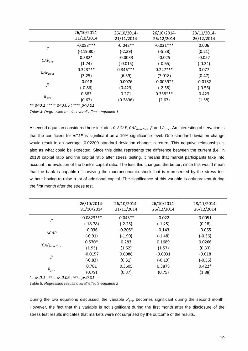
The first equation discussed contains 𝐶, 𝐶𝐴𝑃𝑝𝑟𝑒, 𝐶𝐴𝑃𝑝𝑜𝑠𝑡 , 𝛽 and 𝑅𝑝𝑟𝑒. The most important result that can be

drawn here is that 𝐶𝐴𝑃𝑝𝑜𝑠𝑡 is significant on a 1% significance level the first two months after the date the

stress test results are released. However, when looking more in detail, this significance disappears when

excluding the first month. In other words, markets incorporated the result of the stress test during the first

month after the moment these results became available. Looking at a week-by-week analysis, it becomes

clear that in each week this variable remains significant, with an impact fluctuating between 0.015 and

0.032 standard deviation. The sign of the impact is as what could be expected: a better result from the

stress test leads to a better response of the markets. From this we can conclude that on a 1%

significance level, the null hypothesis �̅� = 0 can be rejected for 𝐶𝐴𝑃𝑝𝑜𝑠𝑡 during the first month after the

release of the stress test results.

19

26/10/2014-31/10/2014

26/10/2014-21/11/2014

26/10/2014-26/12/2014

28/11/2014-26/12/2014

𝐶 -0.083*** -0.042** -0.021*** 0.006

(-119.80) (-2.39) (-5.38) (0.21)

𝐶𝐴𝑃𝑝𝑟𝑒 0.382* -0.0033 -0.025 -0.052

(1.74) (-0.015) (-0.65) (-0.24)

𝐶𝐴𝑃𝑝𝑜𝑠𝑡 0.323*** 0.346*** 0.227*** 0.077

(3.25) (6.39) (7.018) (0.47)

𝛽 -0.018 0.0076 -0.0039** -0.0182

(-0.86) (0.423) (-2.58) (-0.56)

𝑅𝑝𝑟𝑒 0.583 0.271 0.338*** 0.423

(0.62) (0.2896) (2.67) (1.58) *= p<0.1 ; ** = p<0.05 ; ***= p<0.01

Table 4: Regression results overall effects-equation 1

A second equation considered here includes 𝐶, ∆𝐶𝐴𝑃, 𝐶𝐴𝑃𝑏𝑎𝑠𝑒𝑙𝑖𝑛𝑒 , 𝛽 and 𝑅𝑝𝑟𝑒. An interesting observation is

that the coefficient for ∆𝐶𝐴𝑃 is significant on a 10% significance level. One standard deviation change

would result in an average -0.02209 standard deviation change in return. This negative relationship is

also as what could be expected. Since this delta represents the difference between the current (i.e. in

2013) capital ratio and the capital ratio after stress testing, it means that market participants take into

account the evolution of the bank’s capital ratio. The less this changes, the better, since this would mean

that the bank is capable of surviving the macroeconomic shock that is represented by the stress test

without having to raise a lot of additional capital. The significance of this variable is only present during

the first month after the stress test.

26/10/2014-31/10/2014

26/10/2014-21/11/2014

26/10/2014-26/12/2014

28/11/2014-26/12/2014

𝐶 -0.0823*** -0.043** -0.022 0.0051

(-18.78) (-2.25) (-1.25) (0.18)

∆𝐶𝐴𝑃 -0.036 -0.205* -0.143 -0.065

(-0.91) (-1.90) (-1.48) (-0.36)

𝐶𝐴𝑃𝑏𝑎𝑠𝑒𝑙𝑖𝑛𝑒 0.570* 0.283 0.1689 0.0266

(1.95) (1.62) (1.57) (0.33)

𝛽 -0.0157 0.0088 -0.0031 -0.018

(-0.83) (0.51) (-0.19) (-0.56)

𝑅𝑝𝑟𝑒 0.781 0.3605 0.3878 0.422*

(0.79) (0.37) (0.75) (1.88) *= p<0.1 ; ** = p<0.05 ; ***= p<0.01 Table 5: Regression results overall effects-equation 2

During the two equations discussed, the variable 𝑅𝑝𝑟𝑒 becomes significant during the second month.

However, the fact that this variable is not significant during the first month after the disclosure of the

stress test results indicates that markets were not surprised by the outcome of the results.

20

Distinction between vulnerable and other countries

Next to factors that are bank-specific, there might also be external factors that determine the market

reaction to the stress test results. One of these factors could be the country where the bank is located in.

For this model, we focus on the banks located in the Eurozone. We take a look at the influence of the

stress test according to whether a bank is headquartered in a so-called vulnerable country or not. The

distinction between vulnerable and other countries is based on the distinction made by the ECB, for

example in its Financial Stability Review of November 2014 (ECB, 2014c). The countries defined as

vulnerable are Cyprus, Greece, Ireland, Italy, Portugal, Slovenia and Spain. Because of this setup, the

significance levels are now determined using the two-tailed critical values for 10 and 26 degrees of

freedom for non-vulnerable and vulnerable countries respectively. There is a different influence of the

stress test results on these two groups. For banks headquartered in non-vulnerable countries, 𝐶𝐴𝑃𝑝𝑟𝑒 and

𝐶𝐴𝑃𝑝𝑜𝑠𝑡 are both significant on a 1% significance level for the first week after the release of the stress test

results. After this week, this significance disappears. When we look at the impact of both of the variables,

we can see that 𝐶𝐴𝑃𝑝𝑟𝑒 has a positive influence of on average 0.002 standard deviation, while 𝐶𝐴𝑃𝑝𝑜𝑠𝑡

has a negative influence of on average -0.015 standard deviation. Looking at the second equation, ∆𝐶𝐴𝑃

and 𝐶𝐴𝑃𝑏𝑎𝑠𝑒𝑙𝑖𝑛𝑒 are statistically significant (on a 1% and 5% significance level respectively) for the same

time period of one week after the release date of the results. These two variables positively influence the

banks’ stock return with on average 0.003 and 0.012 standard deviations respectively.

26/10/2014-31/10/2014

26/10/2014-21/11/2014

26/10/2014-26/12/2014

𝐶 0.0134 0.011* -0.005

(1.73) (1.86) (-0.53)

𝐶𝐴𝑃𝑝𝑟𝑒 0.085*** 0.0402 0.162

(4.39) (0.27) (1.32)

𝐶𝐴𝑃𝑝𝑜𝑠𝑡 -0.196*** -0.093 -0.116

(-3.61) (-1.14) (-1.79)

𝛽 -0.014 -0.00011 -0.006

(-0.69) (-0.006) (-0.56)

𝑅𝑝𝑟𝑒 0.272 0.4901 0.7849*

(0.52) (1.26) (1.99)

*= p<0.1 ; ** = p<0.05 ; ***= p<0.01 Table 6: Regression results non-vulnerable countries-equation 1

21

26/10/2014-31/10/2014

26/10/2014-21/11/2014

26/10/2014-26/12/2014

𝐶 -0.0156* 0.004 -0.006

(-2.04) (0.42) (-0.59)

∆𝐶𝐴𝑃 0.1042*** 0.0594 0.1344

(4.53) (0.54) (1.47)

𝐶𝐴𝑃𝑏𝑎𝑠𝑒𝑙𝑖𝑛𝑒 0.1506** 0.0171 0.0427

(2.59) (0.27) (0.73)

𝛽 -0.012 0.00002 -0.006

(-0.60) (0.002) (-0.53)

𝑅𝑝𝑟𝑒 -0.002 0.449 0.7274

(-0.005) (1.14) (1.78)

*= p<0.1 ; ** = p<0.05 ; ***= p<0.01

Table 7: Regression results non-vulnerable countries-equation 2

Concerning the vulnerable countries, different observations can be made. Here, 𝐶𝐴𝑃𝑝𝑜𝑠𝑡 is significantly

positive from the third week after the release of the stress test results until the end of the month. On a

monthly level the return is positively influenced with on average 0.161 standard deviation. This economic

relevance is much higher than with non-vulnerable countries and has an opposite sign. At first sight, there

is a significant influence in the second month after the release of the results as well. However, when

filtering out the first month, this significance disappears, indicating that only during the first month after the

release date the markets process this information. This finding is in line with the previous findings

mentioned in the paragraphs dealing with the overall effects.

26/10/2014-31/10/2014

26/10/2014-21/11/2014

26/10/2014-26/12/2014

𝐶 -0.128** -0.055 -0.022

(-3.05) (-1.62) (-0.68)

𝐶𝐴𝑃𝑝𝑟𝑒 0.5193 -0.171 -0.213

(0.51) (-0.37) (-0.65)

𝐶𝐴𝑃𝑝𝑜𝑠𝑡 0.188 0.445** 0.344**

(0.49) (2.76) (2.71)

𝛽 -0.0006 0.0189 0.0019

(-0.01) (0.77) (0.085)

𝑅𝑝𝑟𝑒 1.276 0.574 0.3788

(0.55) (0.38) (0.43) *= p<0.1 ; ** = p<0.05 ; ***= p<0.01 Table 8: Regression results vulnerable countries-equation 1

22

Fama-French grouping

In their paper, Fama and French (1992) formed their portfolios based on size and β, to show the influence

of both variables on the return. Similarly, we could form groups of banks based upon β and 𝐶𝐴𝑃𝑝𝑜𝑠𝑡,

which can give an extra indication of how these variables have an influence on the banks’ return and over

what time period this influence remains.

a. Qualitative approach

As a first step the banks are grouped according to β, 𝐶𝐴𝑃𝑝𝑜𝑠𝑡 and both together. For both variables five

grouping categories are made. In case of β, all banks are evenly divided over the five categories, while for

𝐶𝐴𝑃𝑝𝑜𝑠𝑡 the banks are divided according to their performance in the stress test. The first group contains

banks that have a negative capital ratio after stress testing (5 banks), the second group banks that have a

positive capital ratio after stress testing but still not above the threshold capital ratio (10 banks). The other

groups contain banks that have a capital ratio above the threshold level (14 banks for groups 3 and 4,

and 15 banks for group 5). In the case where both variables are used as grouping variables, only two

groups are made from 𝐶𝐴𝑃𝑝𝑜𝑠𝑡 given the small amount of data. The resulting tables are as follows.

26/10/2014-21/11/2014 Beta group 1 Beta group 2 Beta group 3 Beta group 4 Beta group 5

return -0.018 0.00296 0.008 -0.0018 -0.0224

β 0.44 0.84 1.12 1.290 1.82

𝐶𝐴𝑃𝑝𝑟𝑒 0.125 0.138 0.105 0.109 0.096

𝐶𝐴𝑃𝑝𝑜𝑠𝑡 0.087 0.108 0.072 0.078 0.045

𝐶𝐴𝑃𝑏𝑎𝑠𝑒𝑙𝑖𝑛𝑒 0.137 0.147 0.109 0.110 0.087

𝑅𝑝𝑟𝑒 -0.00018 0.838 0.0059 0.0026 -0.0025

∆𝐶𝐴𝑃 0.038 0.030 0.0333 0.031 0.050

Table 9: Qualitative analysis of grouping banks according to β (average values)

26/10/2014-21/11/2014 Cap(post) group 1

cap(post) group 2

cap(post) group 3

cap(post) group 4

cap(post) group 5

return -0.063 -0.0134 -0.004 0.002 0.005

β 1.62 1.35 1.13 1.14 0.84

𝐶𝐴𝑃𝑝𝑟𝑒 0.063 0.102 0.113 0.111 0.149

𝐶𝐴𝑃𝑝𝑜𝑠𝑡 -0.0196 0.038 0.08 0.089 0.128

𝐶𝐴𝑃𝑏𝑎𝑠𝑒𝑙𝑖𝑛𝑒 0.051 0.087 0.112 0.117 0.162

𝑅𝑝𝑟𝑒 -0.015 0.000002 0.0032 0.004 0.005

∆𝐶𝐴𝑃 0.082 0.063 0.033 0.025 0.021

Table 10: Qualitative analysis of grouping banks according to stress test result (average values)

23

26/10/2014-21/11/2014 Beta group 1 Beta group 2 Beta group 3 Beta group 4 Beta group 5

Average return

Cap(post) group 1 -0.037 0.001 0.002 -0.006 -0.025

Cap(post) group 2 -0.002 0.005 0.013 0.002 -0.020

Table 11: Qualitative analysis of grouping banks according to β and stress test result (average values)

From Table 9 we can see that, at first sight, there is no clear link between the return and β. We do not go

deeper into this in this section, given that the focus here lies on the capital ratio-related variables.

Table 10 tells us more in this respect: as can be seen from the table, the return clearly rises with the

𝐶𝐴𝑃𝑝𝑜𝑠𝑡 group. Furthermore, also 𝑅𝑝𝑟𝑒 increases with this grouping variable. This might indicate that there

is a relation between the average return of the banks two years in advance of the stress test and their

resistance to the shocks to which the banks are exposed during the stress test. It is also clear that there

is a positive relation between 𝐶𝐴𝑃𝑝𝑜𝑠𝑡 and 𝐶𝐴𝑃𝑝𝑟𝑒, which could be expected: the higher the capital ratio

before stress testing, the better the results of the test would be, given the higher initial resistance to

unexpected losses. Also 𝐶𝐴𝑃𝑏𝑎𝑠𝑒𝑙𝑖𝑛𝑒 has a positive relation with 𝐶𝐴𝑃𝑝𝑜𝑠𝑡. However, it is more likely that this

is due to the influence of 𝐶𝐴𝑃𝑝𝑟𝑒 on both 𝐶𝐴𝑃𝑝𝑜𝑠𝑡 and 𝐶𝐴𝑃𝑏𝑎𝑠𝑒𝑙𝑖𝑛𝑒 .

The third table (Table 11) groups the banks first according their β and within these groups according to

𝐶𝐴𝑃𝑝𝑜𝑠𝑡. This grouping considers whether the influence of 𝐶𝐴𝑃𝑝𝑜𝑠𝑡 on the average return is different

according to the size of β. Here it appears not to be the case.

b. Quantitative approach

Next to the tables just formed, we could also combine the first approach of the cross-sectional regression

with the grouping categories just discussed. Making cross-sectional regressions for each of the groups

formed by the β, we can again make some observations. These results are based on two-tailed critical

values of the Student’s t-Distribution, with the degrees of freedom (df) mentioned in the tables.

Starting with the equation including 𝐶, 𝐶𝐴𝑃𝑝𝑟𝑒, 𝐶𝐴𝑃𝑝𝑜𝑠𝑡 , 𝛽 and 𝑅𝑝𝑟𝑒, it can be noticed that 𝐶𝐴𝑃𝑝𝑜𝑠𝑡 is

significant during the first month after the release date of the results. However, this significance only

applies during the first two β categories for which 𝛽 < 1 (rejection of 𝐻0 on a 5% and 1% significance level

respectively, with an average impact of 0.69 and 0.14 standard deviation). This might indicate that the

effect of the stress test results on banks’ return was on average most important with banks having a lower

market risk. Again this effect is fully processed by the markets one month after the release date.

24

26/10/2014-28/11/2014

Beta category 1

(df = 9) Beta category 2

(df = 8) Beta category 3

(df = 9) Beta category 4

(df = 9) Beta category 5

(df = 13)

𝐶 -0.076 0.0335 -0.0638 0.0640 -0.0336

(-1.42) (1.56) (-0.51) (0.59) (-0.91)

𝐶𝐴𝑃𝑝𝑟𝑒 -0.303 -0.702*** 0.4467 -0.130 -0.1115

(-0.60) (-10.79) (1.63) (-0.23) (-0.26)

𝐶𝐴𝑃𝑝𝑜𝑠𝑡 0.983** 0.560*** 0.375 0.5315 0.6205

(3.12) (9.01) (1.41) (0.54) (1.66)

𝛽 0.0230 -0.019 0.0140 -0.0732 -0.00524

(0.82) (-0.66) (0.12) (-0.86) (-0.29)

𝑅𝑝𝑟𝑒 -2.966 4.6787 -3.018 0.552 -1.339

(-1.71) (1.43) (-1.25) (0.30) (-0.72)

*= p<0.1 ; ** = p<0.05 ; ***= p<0.01 Table 12: Regression results grouping according to β – equation 1 (26/10-28/11)

26/10/2014-26/12/2014

Beta category 1 (df = 9)

Beta category 2 (df = 8)

Beta category 3 (df = 9)

Beta category 4 (df = 9)

Beta category 5 (df = 13)

𝐶 -0.0365 0.0129 -0.0193 0.0715 -0.0148

(-0.96) (0.83) (-0.16) (1.08) (-0.44)

𝐶𝐴𝑃𝑝𝑟𝑒 -0.1499 -0.424 0.288 -0.323 -0.154

(-0.36) (-1.73) (1.70) (-0.89) (-0.51)

𝐶𝐴𝑃𝑝𝑜𝑠𝑡 0.472 0.376** 0.113 0.518 0.6005*

(1.15) (2.40) (0.38) (0.93) (1.998)

𝛽 0.0071 -0.0103 -0.0083 -0.0704 -0.0141

(0.34) (-0.43) (-0.09) (-1.33) (-0.75)

𝑅𝑝𝑟𝑒 -1.299 2.737 -1.246 0.596 -1.304

(-0.76) (1.34) (-0.77) (0.58) (-1.07)

*= p<0.1 ; ** = p<0.05 ; ***= p<0.01 Table 13: Regression results grouping according to β – equation 1 (26/10-26/12)

For the equation that contains 𝐶, ∆𝐶𝐴𝑃, 𝐶𝐴𝑃𝑏𝑎𝑠𝑒𝑙𝑖𝑛𝑒 , 𝛽 and 𝑅𝑝𝑟𝑒, there is limited evidence for the influence

of one of the variables on the return. Only for the second β category ∆𝐶𝐴𝑃 becomes significant during the

first two months after ST, with an average impact of -0.07 and -0.09 standard deviation respectively.

25

26/10/2014-21/11/2014

Beta category 1

(df = 9) Beta category 2

(df = 8) Beta category 3

(df = 9) Beta category 4

(df = 9) Beta category 5

(df = 13)

𝐶 -0.089 0.0194 -0.109 0.0440 -0.0153

(-1.60) (1.14) (-0.73) (0.38) (-0.44)

∆𝐶𝐴𝑃 -0.538 -0.542*** -0.170 -0.455 -0.517

(-1.36) (-6.49) (-0.73) (-0.52) (-1.44)

𝐶𝐴𝑃𝑏𝑎𝑠𝑒𝑙𝑖𝑛𝑒 0.548 -0.0661 0.940* 0.434 0.256

(1.80) (-1.14) (2.16) (0.95) (0.66)

𝛽 0.0384 -0.0122 0.0357 -0.0618 -0.00355

(1.35) (-0.40) (0.27) (-0.71) (-0.21)

𝑅𝑝𝑟𝑒 -2.748 4.189 -3.344 0.0629 -1.179

(-1.44) (1.08) (-1.17) (0.03) (-0.66)

*= p<0.1 ; ** = p<0.05 ; ***= p<0.01 Table 14: Regression results grouping according to β – equation 2 (26/10-21/11)

26/10/2014-26/12/2014

Beta category 1

(df = 9) Beta category 2

(df = 8) Beta category 3

(df = 9) Beta category 4

(df = 9) Beta category 5

(df = 13)

𝐶 -0.0436 0.00592 -0.0403 0.0588 -0.00002

(-1.17) (0.43) (-0.28) (0.82) (-0.001)

∆𝐶𝐴𝑃 -0.2598 -0.358* -0.0109 -0.523 -0.504*

(-0.68) (-2.26) (-0.05) (-1.04) (-1.81)

𝐶𝐴𝑃𝑏𝑎𝑠𝑒𝑙𝑖𝑛𝑒 0.265 -0.0131 0.455 0.239 0.242

(1.31) (-0.16) (0.98) (0.92) (0.84)

𝛽 0.0143 -0.00686 0.00149 -0.0635 -0.0129

(0.60) (-0.26) (0.01) (-1.16) (-0.68)

𝑅𝑝𝑟𝑒 -1.202 2.486 -1.394 0.126 -1.192

(-0.68) (1.08) (-0.73) (0.12) (-1.00)

*= p<0.1 ; ** = p<0.05 ; ***= p<0.01 Table 15: Regression results grouping according to β – equation 2 (26/10-26/12)

Considering the cross-sectional regressions made using the grouping by 𝐶𝐴𝑃𝑝𝑜𝑠𝑡, we can again make

some observations. For the equation with the variables 𝐶, ∆𝐶𝐴𝑃, 𝐶𝐴𝑃𝑏𝑎𝑠𝑒𝑙𝑖𝑛𝑒 , 𝛽 and 𝑅𝑝𝑟𝑒, , ∆𝐶𝐴𝑃 has a

significantly negative influence on the return for the 𝐶𝐴𝑃𝑝𝑜𝑠𝑡 groups three and five (rejection of 𝐻0 on a

10% and 5% significance level respectively with an average impact of -2.42 and -0.09 standard

deviation), which have a ratio above the threshold level. This significance disappears after the first month.

However, during the second month after the release of the results, ∆𝐶𝐴𝑃 becomes significant in group

four, with the opposite sign and an average impact of 0.12 standard deviation. The negative sign is easy

to understand given that a higher value for ∆𝐶𝐴𝑃 means a worse capital ratio after stress testing. In

groups one and two this variable is not statistically significant. This suggests that for the banks failing the

26

stress test, it is less important how much the capital ratio decreases compared to the original level in

2013. Rather the fact that the banks do not pass the hurdle rate will be of higher importance.

26/10/2014-21/11/2014

Cap(post) cat1 (df = 3)

Cap(post) cat2 (df = 8)

Cap(post) cat3 (df = 12)

Cap(post) cat4 (df = 11)

Cap(post) cat5 (df = 13)

𝐶 -0.0734 -0.0649* 0.00973 -0.0809 -0.0198

(-0.74) (-2.17) (0.07) (-1.40) (-1.16)

∆𝐶𝐴𝑃 -0.514 -0.168 -1.511* 0.293 -0.320**

(-0.29) (-0.44) (-2.11) (1.35) (-2.57)

𝐶𝐴𝑃𝑏𝑎𝑠𝑒𝑙𝑖𝑛𝑒 -0.161 0.780* 0.523 0.606 0.073

(-0.10) (2.03) (0.72) (1.40) (0.66)

𝛽 0.0170 -0.00441 -0.0106 0.00261 0.0204

(1.11) (-0.30) (-0.20) (0.15) (1.09)

𝑅𝑝𝑟𝑒 -2.191 -0.196 -3.440 0.581 0.497

(-0.23) (-0.21) (-1.07) (0.48) (0.32)

*= p<0.1 ; ** = p<0.05 ; ***= p<0.01 Table 16: Regression results grouping according to post-stress test result-equation 2 (26/10-21/11)

26/10/2014-26/12/2014

Cap(post) cat1 (df = 3)

Cap(post) cat2 (df = 8)

Cap(post) cat3 (df = 12)

Cap(post) cat4 (df = 11)

Cap(post) cat5 (df = 13)

𝐶 -0.0580 -0.0464* 0.0107 -0.0570 -0.0190

(-0.89) (-2.26) (0.13) (-1.60) (-1.55)

∆𝐶𝐴𝑃 -0.846 -0.2501 -0.814 0.277* -0.170

(-0.88) (-0.84) (-1.09) (1.85) (-1.33)

𝐶𝐴𝑃𝑏𝑎𝑠𝑒𝑙𝑖𝑛𝑒 0.269 0.730* 0.224 0.402 0.169

(0.32) (2.29) (0.45) (1.45) (1.64)

𝛽 0.00315 -0.0127 -0.0106 -0.00152 -0.0244

(0.14) (-0.88) (-0.34) (-0.12) (-0.96)

𝑅𝑝𝑟𝑒 -3.520 0.116 -1.146 0.716 2.647

(-0.70) (0.19) (-0.55) (1.04) (1.58)

*= p<0.1 ; ** = p<0.05 ; ***= p<0.01 Table 17: Regression results grouping according to post-stress test result-equation 2 (26/10-26/12)

As a final part in the Fama-French section, we make the regressions while grouping the banks for 𝐶𝐴𝑃𝑝𝑜𝑠𝑡

and β. Only little statistical significance is found here, but all of it is found for the highest 𝐶𝐴𝑃𝑝𝑜𝑠𝑡 ratios in

each of the β categories. The significance is furthermore found for the lower and higher β categories, and

consistently negative for ∆𝐶𝐴𝑃. However, given the limited amounts of data to perform the regression with

(3 to 7 elements each time), we should be reluctant to draw any conclusions.

27

5.3. Conclusion

Considering return, we can state that there are statistical grounds to reject the null hypothesis that �̅� = 0

for the variable representing the capital ratio after stress testing and the one representing the difference in

the starting capital ratio and the capital ratio after stress testing. The exact significance level differs, and

the average influence is not the same for all banks. When splitting up according to the market risk and

according to the size of the capital ratio after stress testing, it becomes clear that the latter has a

significantly positive influence for those banks with a lower market risk. The difference in capital ratios at

the start and after stress testing has a significantly negative influence for those banks that passed the

hurdle rate imposed by the supervisor.

Looking at the difference between countries, the influence of the capital ratio after stress has a higher

economic relevance for banks headquartered in vulnerable countries and has a different sign for the two

groups of countries. The sign of the influence is as what could be expected in the vulnerable countries:

markets reward the banks having a higher capital ratio after stress testing. The influence has an opposite

sign for non-vulnerable countries, but is much smaller. For these countries, markets focus more on the

projected capital ratio without stress testing and on the difference between the starting capital ratio and

the one after stress testing.

Importantly, the impact of most of these variables remains significant during one month after the release

date of the stress test results. This indicates that the information is not fully processed from the moment it

becomes available, but continues to be of importance during one month.

28

6. Market risk

Next to the return a bank’s stock offers, its market risk, referred to as β, is also an important element to

consider when evaluating the impact of the stress test on the banks’ stock market performance. We follow

the same structure as for the previous section, starting with the method used, then describing the findings

and finally sum up in a conclusion.

6.1. Methodology

To evaluate the impact the stress test has on the market risk of the banks under consideration, we first

need to determine the evolution of that market risk during a period after the test. There are several ways

to calculate this β. One way is to make use of the CAPM, as elaborated by Sharpe (1964). The slope

resulting from this regression is then the indicator for market risk. Another option to determine β in a more

direct way is by making use of the following formula: 𝛽𝑖,𝑡 =𝐶𝑜𝑣(𝑅𝑚,𝑡,𝑅𝑖,𝑡)

𝜎²𝑚,𝑡, with t a certain period of time. This

β is actually an indication of how much a fluctuation of the market return influences the bank’s return. In

their work, Fama and French (1992) use portfolios of stocks to determine the β. They calculate the market

risk of the portfolio as a whole by determining a monthly return and then make a regression using a

market return as explanatory variable, which therefore takes a similar form as the method using CAPM.

After calculating this portfolio β, they assign this β to each of the stocks in the portfolio. The approach

used in this Master’s Dissertation follows Fama and French, but rather than making portfolios we use the

return of individual stocks in the regression, given the more limited amount of data.

Next to the way in which the market risk is determined, it is also important to consider the period over

which this β is calculated. Here we use an estimation period of five days to determine β with daily data.

More precisely, for each week in our sample period and for each bank, the following regression is made:

𝑅𝑖,𝑡 = 𝐶 + 𝛽𝑖 ∗ 𝑅𝑚,𝑡, with t going from Friday to Friday (weekends excluded).

Once the weekly market risk is determined, we make use of a similar approach as discussed in the

previous section. Having now the weekly β as dependent variable, we again make the cross-sectional

regression with the capital-related variables as independent variables. Next the time series average and t-

statistic are calculated in a similar fashion.

6.2. Results

In line with the previous section, we consider first the overall effect of the capital related variables on the

market risk. Next, we discuss the influence of the same variables when grouping banks according to the

country they are headquartered in, zooming in on the Eurozone. Finally, a grouping in line with Fama and

French is made, where the focus lies this time on the capital ratio after stress testing. The t-values for

determining the significance of results is indicated between brackets in the tables. Similar to section 5,

only the results of the first week, first month and first two months after the stress test release date are

represented as subsequent periods do not change the conclusions made.

29

Overall effects

The significance of the results is determined here using the two-tailed critical values for the Student’s t-

Distribution with df = 56. When looking at the results, it becomes clear that both 𝐶𝐴𝑃𝑝𝑜𝑠𝑡 and 𝐶𝐴𝑃𝑏𝑎𝑠𝑒𝑙𝑖𝑛𝑒

are statistically relevant variables. 𝐶𝐴𝑃𝑝𝑜𝑠𝑡 is relevant on a 5% significance level with an impact of 6.17

standard deviations, which indicates that this variable has a considerable influence on the market risk.

For the months following, the statistical significance disappears if the first month after the release date of

the stress test results is not taken into account. When looking into more detail during this first month, the

significance does not disappear when the first week after the release of the results is filtered out. This

indicates that, similar as in the return section, markets process the information obtained during the first

month.

𝐶𝐴𝑃𝑏𝑎𝑠𝑒𝑙𝑖𝑛𝑒 is the other relevant variable in the model. This variable is relevant on a 1% significance level

for the first month after the release of the results, with an average impact of 31.21 standard deviations.

Also here, this significance disappears for subsequent months when the first month after the publication

of the results is not taken into account. Furthermore, the significance does not disappear earlier than one

month after this publication as well. This is again a confirmation of the statement that markets take on

average one month to process this information.

An interesting observation is the sign of the influence both variables have. Both have a positive influence,

which means that both contribute to the market risk. Thus, a higher projected capital ratio or a higher

capital ratio after stress testing increases β. However, we should be careful with the meaning of the term

market risk. It concerns the extent to which a stock price follows the movement of the market. In this

case, MSCI Europe increased during the period 31/10/2014-28/11/2014, which means that a large (>1) β

indicates that the stock price increases faster than the average of the market. Therefore, a higher capital

ratio after stress testing or a higher projected capital ratio leads to an increase in the stock price, more

than the increase in the market index.

26/10/2014-31/10/2014

26/10/2014-21/11/2014

26/10/2014-26/12/2014

5/12/2014-26/12/2014

𝐶 -0.4278*** -0.221* -0.2419*** -0.268*

(-6.15) (-1.87) (-2.79) (-1.83)

𝐶𝐴𝑃𝑝𝑟𝑒 -0.7862 -1.8053 -0.3767 1.409

(-0.27) (-0.94) (-0.25) (0.59)

𝐶𝐴𝑃𝑏𝑎𝑠𝑒𝑙𝑖𝑛𝑒 7.536*** 6.476*** 4.550** 2.141

(4.48) (3.00) (2.42) (0.68)

𝐶𝐴𝑃𝑝𝑜𝑠𝑡 1.446 2.603** 2.137* 1.555

(0.69) (2.46) (1.85) (0.64)

*= p<0.1 ; ** = p<0.05 ; ***= p<0.01

Table 18: Regression results overall effects – equation 1

30

A second equation contains 𝐶, 𝐶𝐴𝑃𝑏𝑎𝑠𝑒𝑙𝑖𝑛𝑒 and ∆𝐶𝐴𝑃. Opposite to section 5, ∆𝐶𝐴𝑃 is not significant on a

10% significance level or higher. This means that we cannot reject 𝐻0 that �̅� = 0 for this variable. In

contrast, the two variables discussed above have a positive influence on the market risk, which is

expected to lead to a higher return, all else remaining equal. ∆𝐶𝐴𝑃 breaks this relation between market

risk and return.

26/10/2014-31/10/2014

26/10/2014-21/11/2014

26/10/2014-26/12/2014

𝐶 -0.430*** -0.224* -0.248***

(-5.94) (-1.88) (-2.84)

𝐶𝐴𝑃𝑏𝑎𝑠𝑒𝑙𝑖𝑛𝑒 8.110*** 7.170*** 6.081***

(8.56) (4.97) (5.03)

∆𝐶𝐴𝑃 -1.172 -2.272 -1.407

(-0.48) (-1.65) (-1.39)

*= p<0.1 ; ** = p<0.05 ; ***= p<0.01

Table 19: Regression results overall effects – equation 2

Distinction between vulnerable and other countries

Similar to section 5 we can split up the banks under consideration into two groups, according to the

country they are headquartered in. This can indicate whether there are external factors, in this case the

country, that influence the interpretation of the results. We focus on the Eurozone countries, as such the

sample of banks reduces to 41. This results in two-tailed critical values for the Student’s t-Distribution with

11 and 26 degrees of freedom for non-vulnerable and vulnerable countries respectively.

Looking at the non-vulnerable countries, we can see that for the first equation there is a significantly

negative influence of 𝐶𝐴𝑃𝑝𝑟𝑒 and 𝐶𝐴𝑃𝑝𝑜𝑠𝑡, and a significantly positive influence of 𝐶𝐴𝑃𝑏𝑎𝑠𝑒𝑙𝑖𝑛𝑒 on the

market risk. In other words, the market risk reduces with increasing capital ratio before stress testing and

increasing capital ratio after stress testing, but increases with increasing projected capital ratio without

stress testing. In line with the other results, the significance is valid during the first month after the release

of the stress test results.

The second equation indicates that the variables ∆𝐶𝐴𝑃 and 𝐶𝐴𝑃𝑏𝑎𝑠𝑒𝑙𝑖𝑛𝑒 have a positive influence on the

market risk. Here as well, the influence remains during the first month, after which it disappears. The fact

that 𝐶𝐴𝑃𝑏𝑎𝑠𝑒𝑙𝑖𝑛𝑒 and ∆𝐶𝐴𝑃 have a positive influence can be explained in a similar fashion as before: it

might indicate that a higher projected capital ratio leads to a higher increase in stock prices relative to the

market index. However, this would imply that the opposite is true for 𝐶𝐴𝑃𝑝𝑟𝑒 and 𝐶𝐴𝑃𝑝𝑜𝑠𝑡. A possible

explanation could be that, for non-vulnerable countries, markets are less concerned about the stress test

results but more about profitability, given that a higher capital ratio reduces the return on equity.

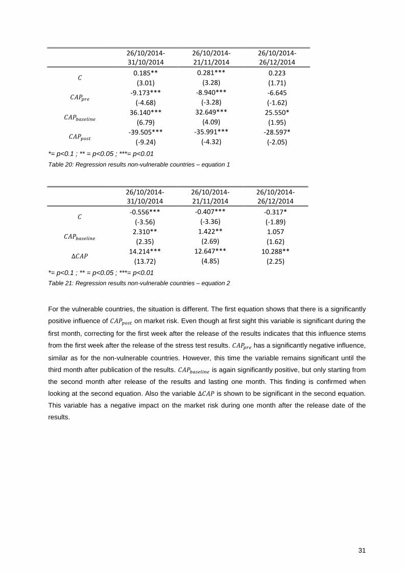
31

26/10/2014-31/10/2014

26/10/2014-21/11/2014

26/10/2014-26/12/2014

𝐶 0.185** 0.281*** 0.223

(3.01) (3.28) (1.71)

𝐶𝐴𝑃𝑝𝑟𝑒 -9.173*** -8.940*** -6.645

(-4.68) (-3.28) (-1.62)

𝐶𝐴𝑃𝑏𝑎𝑠𝑒𝑙𝑖𝑛𝑒 36.140*** 32.649*** 25.550*

(6.79) (4.09) (1.95)

𝐶𝐴𝑃𝑝𝑜𝑠𝑡 -39.505*** -35.991*** -28.597*

(-9.24) (-4.32) (-2.05)

*= p<0.1 ; ** = p<0.05 ; ***= p<0.01

Table 20: Regression results non-vulnerable countries – equation 1

26/10/2014-31/10/2014

26/10/2014-21/11/2014

26/10/2014-26/12/2014

𝐶 -0.556*** -0.407*** -0.317*

(-3.56) (-3.36) (-1.89)

𝐶𝐴𝑃𝑏𝑎𝑠𝑒𝑙𝑖𝑛𝑒 2.310** 1.422** 1.057

(2.35) (2.69) (1.62)

∆𝐶𝐴𝑃 14.214*** 12.647*** 10.288**

(13.72) (4.85) (2.25)

*= p<0.1 ; ** = p<0.05 ; ***= p<0.01

Table 21: Regression results non-vulnerable countries – equation 2

For the vulnerable countries, the situation is different. The first equation shows that there is a significantly

positive influence of 𝐶𝐴𝑃𝑝𝑜𝑠𝑡 on market risk. Even though at first sight this variable is significant during the

first month, correcting for the first week after the release of the results indicates that this influence stems

from the first week after the release of the stress test results. 𝐶𝐴𝑃𝑝𝑟𝑒 has a significantly negative influence,

similar as for the non-vulnerable countries. However, this time the variable remains significant until the

third month after publication of the results. 𝐶𝐴𝑃𝑏𝑎𝑠𝑒𝑙𝑖𝑛𝑒 is again significantly positive, but only starting from

the second month after release of the results and lasting one month. This finding is confirmed when

looking at the second equation. Also the variable ∆𝐶𝐴𝑃 is shown to be significant in the second equation.

This variable has a negative impact on the market risk during one month after the release date of the

results.

32

26/10/2014-31/10/2014

26/10/2014-21/11/2014

26/10/2014-26/12/2014

7/11/2014-28/11/2014

𝐶 0.127* -0.052 -0.025 -0.114

(1.86) (-0.30) (-0.21) (-0.54)

𝐶𝐴𝑃𝑝𝑟𝑒 -1.596*** -3.574*** -3.099*** -4.057***

(-35.23) (-3.33) (-3.84) (-3.28)

𝐶𝐴𝑃𝑏𝑎𝑠𝑒𝑙𝑖𝑛𝑒 0.231 6.129 4.847** 8.043*

(0.13) (1.67) (2.27) (1.99)

𝐶𝐴𝑃𝑝𝑜𝑠𝑡 2.299*** 1.772** 1.600 1.6176

(24.93) (2.15) (1.38) (1.54)

*= p<0.1 ; ** = p<0.05 ; ***= p<0.01

Table 22: Regression results vulnerable countries – equation 1

26/10/2014-31/10/2014

26/10/2014-21/11/2014

26/10/2014-26/12/2014

𝐶 0.121* -0.0367 -0.0127

(1.78) (-0.22) (-0.11)

𝐶𝐴𝑃𝑏𝑎𝑠𝑒𝑙𝑖𝑛𝑒 0.886 4.449 3.4496**

(0.52) (1.56) (2.16)

∆𝐶𝐴𝑃 -2.0106*** -2.512*** -2.2155**

(-27.55) (-3.26) (-2.42)

*= p<0.1 ; ** = p<0.05 ; ***= p<0.01

Table 23: Regression results vulnerable countries – equation 2

The grouping according to country shows that there is a difference in the way the information about the

stress test is processed between vulnerable and other countries. In both, the capital ratio before stress

testing has a decreasing effect on β, but the influence is more persistent in vulnerable countries. The

effect of the capital ratio after stress testing is opposite in both categories: where it increases market risk

in vulnerable countries, it reduces the β in other countries. The same applies for the difference in capital

ratio before and after stress testing.

Fama-French grouping

Similar to section 5, we can group the banks according to the capital ratio obtained after stress testing.

Group 1 contains the banks that have a negative capital ratio as a result (5 banks), group 2 those with a

positive capital ratio but still below the threshold (10 banks), and groups 3 to 5 those banks with a higher

capital ratio than the threshold (14 banks for group 3 and 4, 15 banks for group 5). The degrees of

freedom for the two-tailed critical values in the Student’s t-distribution can be found in the tables. The

variable 𝐶𝐴𝑃𝑏𝑎𝑠𝑒𝑙𝑖𝑛𝑒 becomes significant for groups 2 to 5 during the first month and only the first month

after release of the stress test results. However, the sign of the coefficient is not consistent: for the groups

2 and 5 this sign is positive whereas for groups 3 and 4 it is negative. We can therefore not see a clear

trend in this variable. The same story applies to the variable ∆𝐶𝐴𝑃: here as well, there are groups having

a significantly positive or significantly negative influence on the market risk, without following a clear

trend.

33

26/10/2014-31/10/2014

Cap(post) cat1 (df = 3)

Cap(post) cat2 (df = 8)

Cap(post) cat3 (df = 12)

Cap(post) cat4 (df = 12)

Cap(post) cat5 (df = 13)

𝐶 0.00624 -2.687*** 1.471 -16.553 1.398**

(0.13) (-12.06) (1.05) (-1.49) (2.51)

𝐶𝐴𝑃𝑝𝑟𝑒 0.0710 -26.434*** 2.372 17.740* -34.343***

(0.50) (-25.95) (0.34) (10.77) (-24.35)

𝐶𝐴𝑃𝑏𝑎𝑠𝑒𝑙𝑖𝑛𝑒 -0.162 70.732*** -9.283 -33.894 16.940***

(-0.38) (16.06) (-1.76) (-1.61) (5.93)

𝐶𝐴𝑃𝑝𝑜𝑠𝑡 0.123 -12.861*** -7.870 220.068 15.173

(0.17) (-7.88) (-0.44) (1.40) (1.41)

*= p<0.1 ; ** = p<0.05 ; ***= p<0.01 Table 24: Regression results grouping according to post-stress test result-equation 1 (26/10-31/10)

26/10/2014-21/11/2014

Cap(post) cat1 (df = 3)

Cap(post) cat2 (df = 8)

Cap(post) cat3 (df = 12)

Cap(post) cat4 (df = 12)

Cap(post) cat5 (df = 13)

𝐶 -0.0072 -2.462*** 1.473 -16.968** 3.073**

(-0.38) (-4.80) (1.16) (-2.81) (2.82)

𝐶𝐴𝑃𝑝𝑟𝑒 -0.329 -25.527*** 6.958 16.914** -36.780***

(-0.74) (-4.64) (1.00) (7.96) (-3.65)

𝐶𝐴𝑃𝑏𝑎𝑠𝑒𝑙𝑖𝑛𝑒 0.644 66.596*** -15.693** -40.077** 22.096**

(1.13) (4.74) (-2.39) (-2.59) (2.19)

𝐶𝐴𝑃𝑝𝑜𝑠𝑡 -0.327 -11.471*** -2.993 234.512** -0.926

(-0.61) (-4.88) (-0.20) (2.63) (-0.10)

*= p<0.1 ; ** = p<0.05 ; ***= p<0.01 Table 25: Regression results grouping according to post-stress test result-equation 1 (26/10-21/11)

26/10/2014-26/12/2014

Cap(post) cat1 (df = 3)

Cap(post) cat2 (df = 8)

Cap(post) cat3 (df = 12)

Cap(post) cat4 (df = 12)

Cap(post) cat5 (df = 13)

𝐶 -0.002264613 -1.988* 0.314 -12.390** 2.252**

(-0.20) (-2.20) (0.30) (-2.68) (2.81)

𝐶𝐴𝑃𝑝𝑟𝑒 -0.0587 -20.322* 2.712 15.050** -27.359***

(-0.21) (-2.19) (0.57) (4.75) (-3.93)

𝐶𝐴𝑃𝑏𝑎𝑠𝑒𝑙𝑖𝑛𝑒 0.327 53.258* -9.993 -30.204** 15.378**

(0.93) (2.18) (-1.67) (-2.74) (2.46)

𝐶𝐴𝑃𝑝𝑜𝑠𝑡 -0.0271 -9.029* 9.342 169.442** 1.338

(-0.08) (-2.01) (0.74) (2.54) (0.28)

*= p<0.1 ; ** = p<0.05 ; ***= p<0.01 Table 26: Regression results grouping according to post-stress test result-equation 1 (26/10-26/12)

34

26/10/2014-31/10/2014

Cap(post) cat1 (df = 3)

Cap(post) cat2 (df = 8)

Cap(post) cat3 (df = 12)

Cap(post) cat4 (df = 12)

Cap(post) cat5 (df = 13)

𝐶 0.00735 -3.164*** 1.268** -1.461 0.958**

(0.14) (-12.41) (2.69) (-1.36) (2.79)

𝐶𝐴𝑃𝑝𝑟𝑒 -0.0991 46.249*** -11.244*** 24.428 3.245

(-0.68) (16.81) (-3.10) (1.36) (0.85)

∆𝐶𝐴𝑃 -0.0273 -9.184*** 3.376 -31.445 -24.727***

(-0.09) (-63.10) (1.41) (-1.01) (-4.05)

*= p<0.1 ; ** = p<0.05 ; ***= p<0.01 Table 27: Regression results grouping according to post-stress test result-equation 2 (26/10-31/10)

26/10/2014-21/11/2014

Cap(post) cat1 (df = 3)

Cap(post) cat2 (df = 8)

Cap(post) cat3 (df = 12)

Cap(post) cat4 (df = 12)

Cap(post) cat5 (df = 13)

𝐶 -0.0110 -2.911*** 1.620** -1.0117** 2.206**

(-0.47)) (-4.79) (2.38) (-2.48) (2.94)

𝐶𝐴𝑃𝑝𝑟𝑒 0.432) 43.544*** -14.280** 21.585** -4.841

(1.47) (4.73) (-2.32) (2.84) (-1.10)

∆𝐶𝐴𝑃 0.00460 -9.285*** 6.234 -35.088* -17.867***

(0.04) (-4.42) (1.39) (-2.06) (-4.18)

*= p<0.1 ; ** = p<0.05 ; ***= p<0.01 Table 28: Regression results grouping according to post-stress test result-equation 2 (26/10-21/11)

26/10/2014-26/12/2014

Cap(post) cat1

(df = 3) Cap(post) cat2

(df = 8) Cap(post) cat3

(df = 12) Cap(post) cat4

(df = 12) Cap(post) cat5

(df = 13)

𝐶 -0.00276 -2.345* 0.760 -0.681* 1.655**

(-0.20) (-2.19) (1.09) (-2.14) (2.69)

𝐶𝐴𝑃𝑝𝑟𝑒 0.299 34.971* -5.696 15.043** -3.211

(1.63) (2.21) (-0.85) (2.40) (-1.06)

∆𝐶𝐴𝑃 -0.0151 -7.437* 0.512 -23.108* -14.306***

(-0.22) (-2.29) (0.11) (-1.92) (-4.82)

*= p<0.1 ; ** = p<0.05 ; ***= p<0.01 Table 29: Regression results grouping according to post-stress test result-equation 2 (26/10-26/12)

For this grouping system, one common trend in all variables is that they are no longer statistically

significant after one month. This again refers to the observation of the fact that the markets need a time

period of on average one month to process the information. Exceptions to this are given in groups 4 and 5

using the variables 𝐶𝐴𝑃𝑝𝑜𝑠𝑡 , 𝐶𝐴𝑃𝑏𝑎𝑠𝑒𝑙𝑖𝑛𝑒 and 𝐶𝐴𝑃𝑏𝑎𝑠𝑒, and group 5 using 𝐶𝐴𝑃𝑏𝑎𝑠𝑒𝑙𝑖𝑛𝑒 and ∆𝐶𝐴𝑃. For those

groups, 𝐶𝐴𝑃𝑏𝑎𝑠𝑒 and ∆𝐶𝐴𝑃 respectively remain significant for the month afterwards as well.

35

6.3. Conclusion

In this section we considered the influence of the ST results on market risk, the so-called β. Overall, we

can state that there is a significantly positive influence of the variables representing the projected capital

ratio without stress testing and the capital ratio after stress on the market risk. This is in contrast to the

variable representing the difference between the capital ratios before and after stress testing, for which

we cannot reject 𝐻0 that �̅� = 0 on a 10% significance level. Interpreting these results has to do with the

meaning of the term market risk, which indicates the extent that stocks follow the movements of a market

index. In this case, a β larger than one for the month after the release of the stress test results indicates

that stock prices increase more than the market index. Therefore, this positive influence indicates that

banks with a higher capital ratio after stress testing and higher projected capital ratio without stress

testing, ceteris paribus, outperform the market index.

When making a distinction between countries, it can be noted that there is a difference between

vulnerable and other countries. For both groups the capital before stress testing has a significantly

negative influence, but the time during which this variable remains important differs between three

months and one month respectively. Furthermore, there is an opposite impact of the capital ratio after

stress testing in vulnerable and other countries, as is the case for the difference in capital ratios before

and after stress testing. This indicates that markets respond differently to stress test results depending on

the country where the bank is headquartered.

Grouping according to whether or not banks passed the hurdle rate and to what extent does not add a lot

of new information, except that for the groups with the highest post-stress testing capital ratios there is

somewhat more persistency in the influence of the results.

In line with the results of section 5, it is clear that a certain time passes before the influence of the stress

test results are processed. In most cases this influence only disappears after one month.

36

7. Volatility

As a final element in this study towards the impact of the 2014 EU-wide stress test, we consider the

impact on the volatility of banks’ stock returns. The same structure as in sections 5 and 6 is followed.

7.1. Methodology

To estimate the volatility, the variance (σ²) of the banks’ stock returns is determined. More precisely, the

weekly variance is considered, calculated as the variance of the daily data during that week. After making

these calculations, the weekly change in σ² is determined as follows: ∆𝜎2 = ln(𝑡) − ln(𝑡−1), where t is the

weekly variance. Next, a cross-sectional regression is made using the same approach as described in

section 5. Here, the relative change in weekly variance is regressed on the independent variables. This

means that the regressions try to capture the influence of the capital related variables on the change in

volatility. To assess the statistical significance of the independent variables, a t-statistic is used again.

7.2. Results

As in the previous sections, several regression models are made. First, we consider the overall effects of

the stress test results on the banks’ stock returns. In a second model, we focus on the banks

headquartered in the Eurozone and distinguish two categories. Finally, we split up the banks according to

β and to the capital ratio after stress testing, in line with Fama and French (1992). The t-values for

determining the significance of results is indicated between brackets in the tables. Here as well, only the

first week, first month and first two months after the release date of the stress test results are reported

since subsequent periods do not change the conclusions made.

Overall effects

Looking at the regression results, we can see that only one variable is statistically significant, namely

𝐶𝐴𝑃𝑝𝑜𝑠𝑡. This significance is determined using two-tailed critical values of the Student’s t-Distribution with

55 degrees of freedom. The significant influence is only present during the first week after the results of

the stress test are released, where having a higher capital ratio after stress test leads, on average, to a

decrease in relative change in volatility with 1.36 standard deviation. This means that the variance in

stock returns is more stable over this period when having a better capital ratio after stress testing.

37

26/10/2014-31/10/2014

26/10/2014-21/11/2014

26/10/2014-26/12/2014

𝐶 -0.103 -0.063 -0.1185

(-0.11) (-0.12) (-0.38)

𝐶𝐴𝑃𝑝𝑟𝑒 -0.580 0.872 -17.585

(-0.08) (0.18) (-0.95)

𝐶𝐴𝑃𝑝𝑜𝑠𝑡 -4.0301*** -2.198 18.577

(-16.84) (-0.59) (0.99)

𝛽 0.0335 -0.1125 0.00582

(0.73) (-0.53) (0.02)

*= p<0.1 ; ** = p<0.05 ; ***= p<0.01 Table 30: Regression results overall effects – equation 1

Distinction between vulnerable and other countries

Similar to previous sections, this regression model contains less banks (namely 41) given the fact that

only banks located in the Eurozone are taken into consideration. Here the critical values of the Student’s

t-Distribution (two-tailed) are used for df = 10 and df = 26, for non-vulnerable and vulnerable countries

respectively.

For banks headquartered in countries categorized as vulnerable, two variables have a statistically

significant influence on the change in volatility. In a first equation 𝐶𝐴𝑃𝑝𝑜𝑠𝑡 has a significantly negative

impact (hence creates a more stable volatility) of on average 8.20 standard deviations. This influence,

similar to findings above, is only significant during the first week after the release of the stress test results.

26/10/2014-31/10/2014

26/10/2014-21/11/2014

26/10/2014-26/12/2014

𝐶 -0.023 -0.403 0.7841

(-0.11) (-0.56) (0.83)

𝐶𝐴𝑃𝑝𝑟𝑒 0.8643 3.3966 -37.020

(0.25) (0.53) (-1.01)

𝐶𝐴𝑃𝑝𝑜𝑠𝑡 -4.768*** -2.8399 29.8828

(-3.92) (-0.52) (1.04)

𝛽 -0.0596 -0.039 0.1967

(-0.11) (-0.11) (0.56)

*= p<0.1 ; ** = p<0.05 ; ***= p<0.01 Table 31: Regression results vulnerable countries – equation 1

In a second equation, it is ∆𝐶𝐴𝑃 that has a statistically positive influence on the relative change in

volatility. It leads to an average increase of the relative change in volatility of 2.97 standard deviations.

Also here, the impact is only found during the first week after release of the stress test results.

38

26/10/2014-31/10/2014

26/10/2014-21/11/2014

26/10/2014-26/12/2014

𝐶 -0.134 -0.597 0.577

(-0.84) (-0.83) (0.65)

∆𝐶𝐴𝑃 3.888*** 3.7302 -30.866

(7.19) (0.71) (-1.01)

𝐶𝐴𝑃𝑏𝑎𝑠𝑒𝑙𝑖𝑛𝑒 -2.269 2.0108 -3.983

(-0.53) (0.60) (-0.65)

𝛽 -0.0716 -0.0247 0.155

(-0.14) (-0.07) (0.49) *= p<0.1 ; ** = p<0.05 ; ***= p<0.01 Table 32: Regression results vulnerable countries – equation 2

A different result is found for banks headquartered in other Eurozone countries. There, no statistical

significant impact is found of the explanatory variables on the relative change in volatility.

26/10/2014-31/10/2014

26/10/2014-21/11/2014

26/10/2014-26/12/2014

𝐶 -0.898 0.4125 0.1595

(-0.18) (0.19) (0.14)

𝐶𝐴𝑃𝑝𝑟𝑒 0.573 -1.605 -2.213

(0.03) (-0.18) (-0.303)

𝐶𝐴𝑃𝑝𝑜𝑠𝑡 -10.2017 -0.638 -2.2808

(-0.87) (-0.06) (-0.34)

𝛽 0.9337 -0.3800 -0.0496

(0.31) (-0.27) (-0.06)

*= p<0.1 ; ** = p<0.05 ; ***= p<0.01 Table 33: Regression results non-vulnerable countries – equation 1

26/10/2014-31/10/2014

26/10/2014-21/11/2014

26/10/2014-26/12/2014

𝐶 0.121 0.492 0.328

(0.07) (0.54) (0.63)

∆𝐶𝐴𝑃 5.532 -0.500 0.650

(0.34) (-0.06) (0.11)

𝐶𝐴𝑃𝑏𝑎𝑠𝑒𝑙𝑖𝑛𝑒 -16.253 -2.4642 -4.8043

(-0.80) (-0.17) (-0.63)

𝛽 0.9116 -0.3853 -0.0984

(0.30) (-0.27) (-0.12)

*= p<0.1 ; ** = p<0.05 ; ***= p<0.01 Table 34: Regression results non-vulnerable countries – equation 2

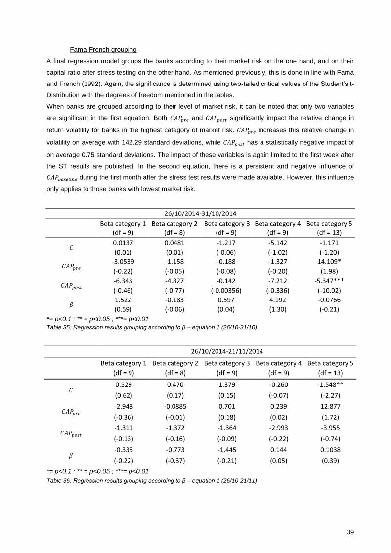
39

Fama-French grouping

A final regression model groups the banks according to their market risk on the one hand, and on their

capital ratio after stress testing on the other hand. As mentioned previously, this is done in line with Fama

and French (1992). Again, the significance is determined using two-tailed critical values of the Student’s t-

Distribution with the degrees of freedom mentioned in the tables.

When banks are grouped according to their level of market risk, it can be noted that only two variables

are significant in the first equation. Both 𝐶𝐴𝑃𝑝𝑟𝑒 and 𝐶𝐴𝑃𝑝𝑜𝑠𝑡 significantly impact the relative change in

return volatility for banks in the highest category of market risk. 𝐶𝐴𝑃𝑝𝑟𝑒 increases this relative change in

volatility on average with 142.29 standard deviations, while 𝐶𝐴𝑃𝑝𝑜𝑠𝑡 has a statistically negative impact of

on average 0.75 standard deviations. The impact of these variables is again limited to the first week after

the ST results are published. In the second equation, there is a persistent and negative influence of

𝐶𝐴𝑃𝑏𝑎𝑠𝑒𝑙𝑖𝑛𝑒 during the first month after the stress test results were made available. However, this influence

only applies to those banks with lowest market risk.

26/10/2014-31/10/2014

Beta category 1

(df = 9) Beta category 2

(df = 8) Beta category 3

(df = 9) Beta category 4

(df = 9) Beta category 5

(df = 13)

𝐶 0.0137 0.0481 -1.217 -5.142 -1.171

(0.01) (0.01) (-0.06) (-1.02) (-1.20)

𝐶𝐴𝑃𝑝𝑟𝑒 -3.0539 -1.158 -0.188 -1.327 14.109*

(-0.22) (-0.05) (-0.08) (-0.20) (1.98)

𝐶𝐴𝑃𝑝𝑜𝑠𝑡 -6.343 -4.827 -0.142 -7.212 -5.347***

(-0.46) (-0.77) (-0.00356) (-0.336) (-10.02)

𝛽 1.522 -0.183 0.597 4.192 -0.0766

(0.59) (-0.06) (0.04) (1.30) (-0.21)

*= p<0.1 ; ** = p<0.05 ; ***= p<0.01 Table 35: Regression results grouping according to β – equation 1 (26/10-31/10)

26/10/2014-21/11/2014

Beta category 1

(df = 9)

Beta category 2

(df = 8)

Beta category 3

(df = 9)

Beta category 4

(df = 9)

Beta category 5

(df = 13)

𝐶 0.529 0.470 1.379 -0.260 -1.548**

(0.62) (0.17) (0.15) (-0.07) (-2.27)

𝐶𝐴𝑃𝑝𝑟𝑒 -2.948 -0.0885 0.701 0.239 12.877

(-0.36) (-0.01) (0.18) (0.02) (1.72)

𝐶𝐴𝑃𝑝𝑜𝑠𝑡 -1.311 -1.372 -1.364 -2.993 -3.955

(-0.13) (-0.16) (-0.09) (-0.22) (-0.74)

𝛽 -0.335 -0.773 -1.445 0.144 0.1038

(-0.22) (-0.37) (-0.21) (0.05) (0.39)

*= p<0.1 ; ** = p<0.05 ; ***= p<0.01

Table 36: Regression results grouping according to β – equation 1 (26/10-21/11)

40

26/10/2014-26/12/2014

Beta category 1

(df = 9) Beta category 2

(df = 8) Beta category 3

(df = 9) Beta category 4

(df = 9) Beta category 5

(df = 13)

𝐶 0,0137 -0,685 10,176 -0,650 -0,161

(0,02) (-0,30) (1,01) (-0,33) (-0,16)

𝐶𝐴𝑃𝑝𝑟𝑒 -3,054 -3,681 -6,630 -3,871 -53,192

(-0,46) (-0,43) (-0,64) (-0,41) (-0,93)

𝐶𝐴𝑃𝑝𝑜𝑠𝑡 -6,343 2,830 -38,947 2,897 54,010

(-0,97) (0,48) (-1,10) (0,28) (1,01)

𝛽 1,522 0,530 -6,909 0,386 1,073

(1,25) (0,27) (-1,02) (0,25) (0,93)

*= p<0.1 ; ** = p<0.05 ; ***= p<0.01 Table 37: Regression results grouping according to β – equation 1 (26/10-26/12)

26/10/2014-31/10/2014

Beta category 1 (df = 9)

Beta category 2 (df = 8)

Beta category 3 (df = 9)

Beta category 4 (df = 9)

Beta category 5 (df = 13)

𝐶 0.0540 3.418 -1.0780 -4.894 1.590

(0.03) (0.79) (-0.06) (-0.91) (0.60)

∆𝐶𝐴𝑃 0.937 -4.537 0.197 3.388 9.248

(0.06) (-0.47) (0.01) (0.24) (0.90)

𝐶𝐴𝑃𝑏𝑎𝑠𝑒𝑙𝑖𝑛𝑒 -6.568* -13.562 -0.715 -8.361 -10.453

(-2.25) (-1.28) (-0.02) (-0.54) (-1.30)

𝛽 1.262 -2.463 0.509 4.088 -0.876

(0.50) (-1.03) (0.04) (1.27) (-0.61)

*= p<0.1 ; ** = p<0.05 ; ***= p<0.01 Table 38: Regression results grouping according to β – equation 2 (26/10-31/10)

26/10/2014-21/11/2014

Beta category 1

(df = 9) Beta category 2

(df = 8) Beta category 3

(df = 9) Beta category 4

(df = 9) Beta category 5

(df = 13)

𝐶 0.809 1.318 1.0083 -0.176 0.549

(0.79) (0.45) (0.11) (-0.05) (0.31)

∆𝐶𝐴𝑃 -1.815 -0.9695 0.714 1.786 -1.0578

(-0.20) (-0.10) (0.08) (0.14) (-0.19)

𝐶𝐴𝑃𝑏𝑎𝑠𝑒𝑙𝑖𝑛𝑒 -4.862*** -3.375 0.4021 -2.662 -4.502

(-4.13) (-0.51) (0.03) (-0.47) (-0.65)

𝛽 -0.4037 -1.347 -1.197 0.10439 -0.185

(-0.29) (-0.62) (-0.17) (0.04) (-0.23)

*= p<0.1 ; ** = p<0.05 ; ***= p<0.01 Table 39: Regression results grouping according to β – equation 2 (26/10/-21/11)

41

26/10/2014-26/12/2014

Beta category 1 (df = 9)

Beta category 2 (df = 8)

Beta category 3 (df = 9)

Beta category 4 (df = 9)

Beta category 5 (df = 13)

𝐶 1.562 -0.0003 16.755 -0.666 -3.121

(1.08) (-0.0001) (1.02) (-0.34) (-0.90)

∆𝐶𝐴𝑃 0.926 -6.015 31.754 -3.646 2.104

(0.15) (-0.93) (1.11) (-0.37) (0.26)

𝐶𝐴𝑃𝑏𝑎𝑠𝑒𝑙𝑖𝑛𝑒 -11.572 -2.431 -62.823 -1.377 18.623

(-1.04) (-0.63) (-1.00) (-0.39) (0.90)

𝛽 -0.520 0.0978 -10.720 0.453 -1.084

(-0.62) (0.05) (-1.04) (0.28) (-0.93)

*= p<0.1 ; ** = p<0.05 ; ***= p<0.01 Table 40: Regression results grouping according to β – equation 2 (26/10-26/12)

Grouped according to the capital ratio after stress testing, no significance is found during the first month

after releasing the stress test results. There is, however, a significantly positive impact the next month of

𝐶𝐴𝑃𝑝𝑜𝑠𝑡 on the relative change in volatility for those banks whose capital ratio after stress testing was

positive, but did not pass the capital threshold. This positive impact, in contrast to the negative impact of

this variable observed otherwise, is most likely due to the fact that the banks did not pass the hurdle rate.

As mentioned, this influence is only noted during this second month, after which it is no longer statistically

significant.

26/10/2014-31/10/2014

Cap(post) cat1 (df = 3)

Cap(post) cat2 (df = 8)

Cap(post) cat3 (df = 12)

Cap(post) cat4 (df = 11)

Cap(post) cat5 (df = 13)

𝐶 1.285 -0.307*** -1.085*** -6.520 0.487

(0.53) (-9.56) (-5.35) (-0.62) (0.19)

𝐶𝐴𝑃𝑝𝑟𝑒 -18.700 -1.587 2.015 4.724 6.975

(-0.39) (-0.68) (0.45) (1.32) (1.25)

𝐶𝐴𝑃𝑝𝑜𝑠𝑡 -16.024 2.500 5.018 46.414 -12.046

(-2.12) (0.99) (0.18) (0.63) (-0.82)

𝛽 -0.189 0.0356 0.0169 1.326 -0.747

(-0.25) (0.17) (0.01) (0.36) (-0.54)

*= p<0.1 ; ** = p<0.05 ; ***= p<0.01 Table 41: Regression results grouping according to post-stress test result–equation 1 (26/10-31/10)

42

26/10/2014-21/11/2014

Cap(post) cat1 (df = 3)

Cap(post) cat2 (df = 8)

Cap(post) cat3 (df = 12)

Cap(post) cat4 (df = 11)

Cap(post) cat5 (df = 13)

𝐶 0.239 -1.202 -0.356 -1.990 0.087

(0.14) (-1.49) (-0.36) (-0.29) (0.06)

𝐶𝐴𝑃𝑝𝑟𝑒 -4.890 5.255 4.806 5.337 -2.088

(-0.21) (0.99) (0.79) (0.86) (-0.41)

𝐶𝐴𝑃𝑝𝑜𝑠𝑡 -9.543 7.299 -6.873 18.406 -0.186

(-0.71) (0.80) (-0.42) (0.35) (-0.02)

𝛽 -0.155 0.052 0.140 -0.369 -0.130

(-0.52) (0.16) (0.23) (-0.21) (-0.18)

*= p<0.1 ; ** = p<0.05 ; ***= p<0.01 Table 42: Regression results grouping according to post-stress test result–equation 1 (26/10-21/11)

26/10/2014-26/12/2014

Cap(post) cat1

(df = 3) Cap(post) cat2

(df = 8) Cap(post) cat3

(df = 12) Cap(post) cat4

(df = 11) Cap(post) cat5

(df = 13)

𝐶 4.912 -1.43* -0.251 -0.0841 -5.686

(1.017) (-1.95) (-0.26) (-0.02) (-0.99)

𝐶𝐴𝑃𝑝𝑟𝑒 -78.907 2.949 3.151 -2.747 23.763

(-1.01) (0.52) (0.52) (-0.34) (1.08)

𝐶𝐴𝑃𝑝𝑜𝑠𝑡 106.113 18.620* -6.911 3.675 16.346

(0.99) (2.02) (-0.64) (0.11) (0.75)

𝛽 0.299 0.0166 0.102 -0.214 -1.099

(0.69) (0.05) (0.26) (-0.22) (-0.92)

*= p<0.1 ; ** = p<0.05 ; ***= p<0.01 Table 43: Regression results grouping according to post-stress test result–equation 1 (26/10/-26/12)

7.3. Conclusion

This section considered whether the 2014 EU-wide stress test results had an impact on the relative

change in banks’ stock return volatility. In general, influence was found mainly during the first week after

release of the results. The capital ratio after stress testing was the most important factor to influence this

relative change in volatility. This variable had a negative impact, meaning that markets reacted positively

to a higher capital ratio after stress testing.

Distinguishing between countries categorized as vulnerable and others within the Eurozone shows that

the impact of the stress test results is mainly located in the vulnerable countries. There, both the capital

ratio after stress testing and the difference in the current capital ratio and the one after stress testing

influenced the relative change in volatility (negatively and positively respectively). In contrast, no

significant impact was found in the other countries, indicating that markets considered the outcome more

important in the vulnerable countries. Again, these influences are only present during one week after the

results of the stress test were released.

43

In a third model, we grouped banks according to their market risk and capital ratio after stress testing. For

those banks with the highest market risk, the capital ratio after stress testing reduced the relative change

in volatility, but the influence is again limited to one week after the results were released. Also for this

category, the capital ratio before stress testing was of positive influence. For those banks with lowest

market risk, a higher projected capital ratio for 2016 without stress testing reduced the relative change in

volatility. Here the impact was noticeable during one month after the release of the results.

Turning to the other grouping category, only for banks that did not pass the stress test but still had a

positive capital ratio after stress testing there is a significant influence to be noted. This influence stems

from the capital ratio after stress testing and is positive here, which is probably due to the fact that banks

did not pass the hurdle rate. This influence is only noted during the second month after the release of the

results.

44

8. Limitations

When describing the results and the conclusions in the previous sections, there are some limitations that

have to be taken into consideration. First of all, due to a smaller dataset, the risk of multicollinearity

increases. This would imply larger confidence intervals since the variance of the estimators increases.

This means that the value of the t-statistics reduces (see, for example, Damodar and Dawn (2009)).

Another issue which is mentioned by Fama and MacBeth (1973) is the often made observation that the

distribution of returns is thick-tailed. When using the assumption of normality, this might imply that the t-

statistics are overestimates. This problem is in part reduced by not using daily but weekly returns in

section 5 since, as mentioned by Frömmel (2011), the kurtosis declines with temporal aggregation. This

more leptokurtic behaviour, along with the degree of multicollinearity, increases the reliability when stating

that a certain variable no longer has a statistically relevant influence, given a certain confidence level.

Nevertheless, it also reduces the strength of statements where the null hypothesis of insignificance is

rejected. Fama and MacBeth (1973) further address this issue and consider overestimated t-statistics not

as a serious problem for their research.

Furthermore, it should be noted that the sample of banks used is relatively small. This is due to the setup

of the research, where in order to be able to look at the market reaction towards banks involved in the

2014 EU-wide stress test, these banks should be both subject to the exercise and listed on the stock

market. The research is also limited to the 2014 EU-wide stress test, which means that one should be

careful in extending these conclusions to other stress tests.

45

9. Conclusion

This Master’s Dissertation aims at considering the impact of the EU-wide stress test conducted in 2014

on bank stock market performance over an extended period of time. The main research question that we

try to answer is therefore: what, if any, long-run impact did the EU-wide 2014 stress test have on the

stock market performance of the banks involved? Here, long-run is considered in a granular way where

we extend the period starting from one week after the stress test release date until the release date of the

results of the 2016 EU-wide stress test. The main research question is subdivided into three separate

questions: (1) What long-run impact did the stress test have on the return of the banks involved?, (2)

What long-run impact did the stress test have on the market risk of the banks involved?, and (3) What

long-run impact did the stress test have on the stock market volatility of the banks involved? Each of

these questions is considered in the sections above. We approached every question using three different

models, each looking from a different point of view to the banks. A first model considers the overall impact

of the stress test results on banks, not making any further distinctions. A second model considers the

impact of the results as well, but groups banks according to whether or not they are located in a

vulnerable country (following the grouping made by the ECB). For this model, only banks headquartered

in the Eurozone are considered. Finally, the third model groups banks according to their market risk and

according to their capital ratio after stress testing. The main results are as follows.

9.1. What long-run impact did the stress test have on the return of the banks

involved?

For the research question considering the return of the banks involved, the first model indicates that the

capital ratio after stress testing on the one hand, and the difference in capital ratio before and after stress

testing on the other, influence the return of banks. While the first capital ratio has a positive impact, the

second one has a negative impact. Both these signs could be expected, since it means that markets react

positively on banks that come out of the test safely (a high capital ratio after stress testing and a small

difference in capital ratio before and after stress testing). The influence of these variables is persistent

during one month after the release of the stress test results. The second model shows us that for

vulnerable countries, the influence of the results lasts one month. For other countries, markets seem to

process the information more quickly since the influence of the results disappears after one week.

Furthermore, this model shows that the information is processed differently according to the type of

country. Where in vulnerable countries the capital ratio after stress testing receives most attention, this is

less the case in other countries where the projected capital ratio without stress testing is of influence.

When looking at the third model, we can observe that especially for banks with lower market risk the

capital ratio after stress testing is of importance. The difference in capital ratios before and after stress

testing is most important for banks that passed the hurdle rate imposed by the supervisor, suggesting that

the first thing markets look at is whether or not this threshold capital ratio is achieved. Again most of the

impact is found during the first month after the release of the stress test results.

46

9.2. What long-run impact did the stress test have on the market risk of the banks

involved?

The release of the stress test results had an impact on the market risk of banks. The first model shows us

that again the capital ratio after stress testing was significant. This ratio has a positive relation with the

market risk. The projected capital ratio without stress testing also shows a statistically significant

contribution to the market risk. Both variables have an impact during one month after the release of the

results. Here, it should be noted that during the month after the release of the stress test results, the

market index MSCI Europe went up. Therefore, the meaning of this positive influence is that the higher

the variable (ceteris paribus) is, the more the stock prices increase relative to the increase of the market

index. The second model indicates that also concerning market risk, there is a difference between

vulnerable and other countries. For both groups, the capital ratio before stress testing is significant and

decreases market risk. For vulnerable countries, this effect lasts longer (namely three months compared

to one month for other countries). Furthermore, for both groups of countries the projected capital ratio

without stress testing is significant and contributes to market risk. The capital ratio after stress testing is

increasing market risk during the first week after the results are released in case of vulnerable countries,

whereas it reduces market risk during one month for other countries. The difference in capital ratio before

and after stress testing shows the reverse pattern: its influence is significantly negative for the first month

in case of vulnerable countries and significantly positive during one month for other countries. The

findings of this second model indicate, as was the case with the return of the banks, that trends in

vulnerable countries are different as in other countries. The third model does not show clear trends, but

confirms the observation that most influence of the results disappears after one month.

9.3. What long-run impact did the stress test have on the stock market volatility of

the banks involved?

The final consideration is the impact of the stress test results on the volatility of the return of banks. In the

first model, a negative influence is to be noted of the capital ratio after stress testing during one week.

The second model confirms the observation of the first model for vulnerable countries. However, here the

change in capital ratio before and after stress testing has an influence as well. This variable increases the

relative change in volatility in the first week after the results are released. For other countries, no

significant influence is found on the relative change in volatility. The third model shows us that for those

banks with the lowest market risk, the projected capital without stress testing has a negative influence on

the relative change in volatility during one month after the results are known. For the banks with a high

market risk, the starting capital ratio increases the relative change in volatility, whereas the capital ratio

after stress testing reduces it. Both influences are significant for the first week after release of the results.

Banks that did not pass the hurdle rate after stress testing, but still ended up with a positive capital ratio,

see their volatility influenced by this capital ratio in the longer term. A consistent message across all three

models is that the capital ratio after stress testing reduces the relative change in volatility, indicating that

markets react positively on better stress test performance.

47

9.4. Main research question: what, if any, long-run impact did the EU-wide 2014

stress test have on the stock market performance of the banks involved?

To conclude, we can address the main research question of this Master’s Dissertation. Having considered

different aspects of stock market performance, we can state that there is indeed a certain long-run impact

of the EU-wide 2014 stress test on this performance. The meaning of the term long-run is now clearer.

For return, market risk and for volatility the general trend is that we can no longer reject null hypotheses

of insignificance from one month after the results of the stress test are released onwards. In other words,

these results influenced the behaviour of markets during one month. The factor of the results having most

influence on markets is the capital ratio after stress testing, which is the main stress test result. In

general, markets responded positively to banks having a better result with regard to this capital ratio.

However, the projected capital ratio without stress testing and the difference in capital ratio before and

after stress testing (more indirect results of the stress test) also influence markets in several aspects.

This research focuses on the 2014 EU-wide stress test. Further research might focus on other stress

tests, in order to determine the extent to which the reaction to the 2014 EU-wide stress test can be

generalized to market reactions on stress tests in general. Furthermore, additional grouping categories

might be interesting to be considered.

I

Bibliography

Acharya, V., Engle, R., & Pierret, D. (2014). Testing macroprudential stress tests: The risk of regulatory

risk weights. Journal of Monetary Economics, 65, 36-53. doi:10.1016/j.jmoneco.2014.04.014

Alves, C., Mendes, V., & da Silva, P. P. (2015). Do stress tests matter? A study on the impact of the

disclosure of stress test results on European financial stocks and CDS markets. Applied

Economics, 47(12), 1213-1229. doi:10.1080/00036846.2014.993132

Andrade, P., Breckenfelder, J. H., De Fiore, F., Karadi, P., & Tristani, O. (2016). The ECB's asset

purchase programme: an early assessment.

BIS. (s.d.-a). Basel Process. Retrieved from https://www.bis.org/about/basel_process.htm

BIS. (s.d.-b). Promoting global monetary and financial stability through international cooperation.

Retrieved from https://www.bis.org/about/functions.htm?m=1%7C3

Camara, B., Pessarossi, P., & Philippon, T. (2016). Back-testing bank stress tests.

Candelon, B., & Sy, A. N. (2015). How Did Markets React to Stress Tests? : International Monetary Fund.

CEBS. (2009). CEBS's press release on the results of the EU-wide stress testing exercise [Press

release]. Retrieved from http://www.eba.europa.eu/documents/10180/15977/CEBS-2009-180-

Annex-2-%28Press-release-from-CEBS%29.pdf

CEBS. (2010). Aggregate outcome of the 2010 EU wide stress test exercise coordinated by CEBS in

cooperation with the ECB. In: Committee of European Banking Supervisors.

Cochrane, J. H. (2009). Asset Pricing:(Revised Edition): Princeton university press.

Damodar, N. G., & Dawn, C. P. (2009). Basic Econometrics (5th ed.): McGraw-Hill/Irwin.

EBA. (2011). European Banking Authority - 2011 EU-wide stress test - aggregate report. In: European

Banking Authority.

EBA. (2014a). EBA publishes 2014 EU-wide stress test results [Press release]. Retrieved from

http://www.eba.europa.eu/-/eba-publishes-2014-eu-wide-stress-test-results

EBA. (2014b). Main features of the 2014 EU-wide stress test. In: European Banking Authority.

EBA. (2014c). Results of 2014 EU-wide stress test. Retrieved from

http://www.eba.europa.eu/documents/10180/851779/2014+EU-wide+ST-aggregate+results.pdf

EBA. (2015). EBA announces details of 2016 EU-wide stress test [Press release]. Retrieved from

http://www.eba.europa.eu/-/eba-announces-details-of-2016-eu-wide-stress-

test?doAsGroupId=10180

EBA. (2016a). 2016 EU-Wide Stress Test - Methodological Note. Retrieved from

http://www.eba.europa.eu/documents/10180/1259315/2016+EU-wide+stress+test-

Methodological+note.pdf

EBA. (2016b). EBA publishes 2016 EU-wide stress test results [Press release]. Retrieved from

http://www.eba.europa.eu/-/eba-publishes-2016-eu-wide-stress-test-results

EBA. (2016c). The European Banking Authority at a glance. In: European Banking Authority.

EBA. (s.d.). About us. Retrieved from https://www.eba.europa.eu/about-us

II

ECB. (2014a). Aggregate report on the comprehensive assessment. In. Frankfurt am Main: European

Central Bank.

Decision of the European Central Bank of 31 January 2014 on the close cooperation with the national

competent authorities of participating Member States whose currency is not the euro, (2014b).

ECB. (2014c). Financial Stability Review - November 2014. In. Frankfurt am Main: European Central

Bank.

ECB. (2014d). Guide to banking supervision. In. Frankfurt am Main: European Central Bank.

ECB. (2014e). Results of the 2014 comprehensive assessment. Retrieved from

https://www.bankingsupervision.europa.eu/banking/comprehensive/2014/html/index.en.html

ECB. (2017). Joint Supervisory Teams. Retrieved from

https://www.bankingsupervision.europa.eu/banking/approach/jst/html/index.en.html

ESRB. (2014). EBA/SSM stress test: The macroeconomic adverse scenario. In: European Systemic Risk

Board.

European Commission. (2014). European Commission projections for the 2014 EU-wide stress tests

baseline scenario. Retrieved from

https://www.eba.europa.eu/documents/10180/669262/EC+projections.pdf

Fama, E., & French, K. (1992). The cross-section of expected stock returns. Journal of Finance, 47(2),

427-465. doi:10.2307/2329112

Fama, E., & MacBeth, J. (1973). Risk, return, and equilibrium - Empirical tests. Journal of Political

Economy, 81(3), 607-636. doi:10.1086/260061

Fritz-Morgenthal, S., Hellmuth, J., & Packham, N. (2016). Does risk culture matter? The relationship

between risk culture indicators and stress test results. Journal of Risk Management in Financial

Institutions, 9(1), 71-84.

Frömmel, M. (2011). Portfolios and investments (2nd ed.). Norderstedt: Books on demand.

Gerhardt, M., & Vander Vennet, R. (2017). European bank stress test and sovereign exposures. Applied

Economics Letters, 24(14), 972-976. doi:10.1080/13504851.2016.1243208

Goldstein, I., & Sapra, H. (2014). Should banks' stress test results be disclosed? An analysis of the costs

and benefits. Foundations and Trends® in Finance, 8(1), 1-54.

Gros, D. (2012). The Single European Market in Banking in decline – ECB to the rescue? In T. Beck

(Ed.), Banking Union for Europe - Risks and challenges. London: Centre for Economic Policy

Research.

Pattipeilohy, C., Van Den End, J. W., Tabbae, M., Frost, J., & De Haan, J. (2013). Unconventional

monetary policy of the ECB during the financial crisis: An assessment and new evidence.

Petrella, G., & Resti, A. (2013). Supervisors as information producers: Do stress tests reduce bank

opaqueness? Journal of Banking & Finance, 37(12), 5406-5420.

doi:10.1016/j.jbankfin.2013.01.005

Pill, H., & Reichlin, L. (2014). Exceptional policies for exceptional times: the ECB's response to the rolling

crises of the Euro Area, and how it has brought us towards a new grand bargain. In. London:

Centre for Economic Policy Research.

III

Quaglia, L. (2013). Financial regulation and supervision in the European Union after the crisis. Journal of

Economic Policy Reform, 16(1), 17-30.

Sahin, C., & de Haan, J. (2016). Market reactions to the ECB's Comprehensive Assessment. Economics

Letters, 140, 1-5. doi:10.1016/j.econlet.2015.12.011

Schuermann, T. (2014). Stress testing banks. International Journal of Forecasting, 30(3), 717-728.

Sharpe, W. F. (1964). Capital asset prices: A theory of market equilibrium under conditions of risk. The

journal of finance, 19(3), 425-442.