Bank of Canada Banque du Canada

Working Paper 2005-22 / Document de travail 2005-22

The Effects of the Exchange Rate onInvestment: Evidence from Canadian

Manufacturing Industries

by

Tarek Harchaoui, Faouzi Tarkhani, and Terence Yuen

ISSN 1192-5434

Printed in Canada on recycled paper

Bank of Canada Working Paper 2005-22

August 2005

The Effects of the Exchange Rate onInvestment: Evidence from Canadian

Manufacturing Industries

by

Tarek Harchaoui,1 Faouzi Tarkhani,1 and Terence Yuen2

1Micro-Economic Analysis DivisionStatistics Canada

Ottawa, Ontario, Canada K1A 0T6tarek.harchaoui@statcan.cafaouzi.tarkhani@statcan.ca

2Research DepartmentBank of Canada

Ottawa, Ontario, Canada K1A 0G9tyuen@bankofcanada.ca

The views expressed in this paper are those of the authors.No responsibility for them should be attributed to the Bank of Canada

or Statistics Canada.

iii

Contents

Acknowledgements. . . . . . . . . . . . . . . . . . . . . . . . . . . . . . . . . . . . . . . . . . . . . . . . . . . . . . . . . . . . ivAbstract/Résumé. . . . . . . . . . . . . . . . . . . . . . . . . . . . . . . . . . . . . . . . . . . . . . . . . . . . . . . . . . . . . . . v

1. Introduction . . . . . . . . . . . . . . . . . . . . . . . . . . . . . . . . . . . . . . . . . . . . . . . . . . . . . . . . . . . . . . 1

2. Theoretical Framework . . . . . . . . . . . . . . . . . . . . . . . . . . . . . . . . . . . . . . . . . . . . . . . . . . . . . 3

2.1 The effects of the exchange rate on investment . . . . . . . . . . . . . . . . . . . . . . . . . . . . . . 3

2.2 Different investment sensitivity to exchange rates across industries . . . . . . . . . . . . . . 9

3. Data . . . . . . . . . . . . . . . . . . . . . . . . . . . . . . . . . . . . . . . . . . . . . . . . . . . . . . . . . . . . . . . . . . . 11

4. Empirical Estimation . . . . . . . . . . . . . . . . . . . . . . . . . . . . . . . . . . . . . . . . . . . . . . . . . . . . . . 13

4.1 Total investment . . . . . . . . . . . . . . . . . . . . . . . . . . . . . . . . . . . . . . . . . . . . . . . . . . . . . 15

4.2 Investment in IT, other M&E, and structures . . . . . . . . . . . . . . . . . . . . . . . . . . . . . . . 20

4.3 Differences across industries . . . . . . . . . . . . . . . . . . . . . . . . . . . . . . . . . . . . . . . . . . . 22

5. Conclusions . . . . . . . . . . . . . . . . . . . . . . . . . . . . . . . . . . . . . . . . . . . . . . . . . . . . . . . . . . . . . 23

References. . . . . . . . . . . . . . . . . . . . . . . . . . . . . . . . . . . . . . . . . . . . . . . . . . . . . . . . . . . . . . . . . . . 26

Tables . . . . . . . . . . . . . . . . . . . . . . . . . . . . . . . . . . . . . . . . . . . . . . . . . . . . . . . . . . . . . . . . . . . . . . 29

Figures. . . . . . . . . . . . . . . . . . . . . . . . . . . . . . . . . . . . . . . . . . . . . . . . . . . . . . . . . . . . . . . . . . . . . . 41

Appendix A. . . . . . . . . . . . . . . . . . . . . . . . . . . . . . . . . . . . . . . . . . . . . . . . . . . . . . . . . . . . . . . . . . 47

Appendix B . . . . . . . . . . . . . . . . . . . . . . . . . . . . . . . . . . . . . . . . . . . . . . . . . . . . . . . . . . . . . . . . . . 49

iv

Acknowledgements

We have benefited from discussions with Bob Amano, John Baldwin, Allan Crawford, Bob Fay,

Eric Santor, and Paul Warren. We thank Nadja Kamhi for excellent research assistance.

v

Abstract

Using industry-level data for 22 Canadian manufacturing industries, the authors examine the

relationship between exchange rates and investment during the period 1981–97. Their empirical

results show that the overall effect of exchange rates on total investment is statistically

insignificant. Further investigation reveals the non-uniform investment response to exchange rate

movements in three channels. First, it is important to distinguish between environments that have

low and high exchange rate volatilities. Through changes in output demands, depreciations would

have a positive effect on total investment when the exchange rate volatility is low. Yet, this

stimulative effect becomes considerably smaller as the volatility increases. Second, these results

for total investment are mainly due to movements in other machinery and equipment, and not to

investment in information technology and structures. Third, investment in industries with low

markup ratios are more likely to be affected by exchange rate movements.

JEL classification: F4, D24Bank classification: Exchange rates; Domestic demand and components

Résumé

À l’aide de données sectorielles se rapportant à 22 branches industrielles canadiennes, les auteurs

étudient le lien entre l’évolution du taux de change et l’investissement de 1981 à 1997. D’après

leurs résultats empiriques, l’effet global des mouvements de change sur le volume total des

investissements n’est pas significatif sur le plan statistique. Un examen plus approfondi révèle que

l’investissement ne réagit pas de façon uniforme aux variations du taux de change. D’abord, il

importe de distinguer les périodes où la volatilité de ce dernier est faible et celles où elle est

élevée. Durant les périodes de faible volatilité, les dépréciations ont une incidence favorable sur

l’investissement total en provoquant des modifications de la demande de produits. Toutefois, cette

incidence diminue nettement avec l’augmentation de la volatilité. Deuxième constat : l’effet

observé concerne essentiellement le segment autres machines et matériel, les investissements

consacrés aux technologies de l’information et aux installations étant peu affectés.

Troisièmement, dans les branches où les taux de marge sont bas, l’investissement tend à être plus

sensible aux fluctuations du taux de change.

Classification JEL : F4, D24Classification de la Banque : Taux de change; Demande intérieure et composantes

1. Introduction

Exchange rate movements have important implications for a wide range of

economic variables. While a continuous effort has been made to improve our

understanding of the exchange rate pass-through on prices (e.g., Taylor 2000) and

profitability (e.g., Bodnar, Dumas, and Marston 2002), some recent studies have

extended the analysis by examining the impact of exchange rate movements on the real

economy. In particular, one research stream focuses on the relationship between

exchange rate fluctuations and investment (e.g., Campa and Goldberg 1999). In theory,

changes in the exchange rate have two opposite effects on investment. When the

domestic currency depreciates, the marginal profit of investing an additional unit of

capital is likely to increase, because there are higher revenues from both domestic and

foreign sales. Yet, this positive effect is counterbalanced by the rising variable cost and

the higher price for imported capital. Theoretical models provide no clear indication as to

which effect is dominant. The overall effect of exchange rates on investment remains an

empirical question.

Goldberg (1993) fmds that a real depreciation (appreciation) of the U.S. dollar

was likely to generate an expansion (reduction) in investment in the 1970s, but that the

opposite pattern prevailed during the 1980s. Campa al'ld Goldberg (1995) attribute this

difference in investment response between the 1970s and 1980s to the decline in industry

export exposure as U.S. firms progressively increased their reliance on imported inputs.

Furthermore, their empirical fmdings show distinct investment patterns across industries

with different price-over-cost markup ratios. They fmd that investment in high-markup

industries with an oligopolistic market structure is less responsive to exchange rates.

Most of the empirical investigations in this area are based on data from U.S.

manufacturing industries. The literature provides very limited evidence for other

countries. A recent cross-country study by Campa and Goldberg (1999) compares the

investment sensitivity in the United States, United Kingdom, Japan, and Canada for the

period 1970-93. Surprisingly, given the high degree of openness of Canadian

manufacturing industries, investment in Canada turns out to be the least responsive to

exchange rate movements. The vector-autoregressive models in Lafrance and Tessier

1

(2001) also find an insignificant link between the Canadian real exchange rate and

aggregate investment. The conclusions in these two studies pose a challenging question

as to why investment in a small open economy like Canada's would be insulated from

exchange rates.

We shed light on this puzzle by utilizing more disaggregated data at the industry

level for the manufacturing sector, which enables us to explore four main issues

regarding the non-uniformity of the exchange rate effects. First, we examine the different

channels through which exchange rates affect total investment. An exchange rate

depreciation (appreciation) stimulates (dampens) investment by enhancing demands in

both the domestic and export markets, but it reduces (increases) investment because of

the increasing cost of imported intermediate goods and the user cost of capital. Second,

the variability of exchange rates can affect a flml' s perception of whether the shocks are

permanent or transitory. Therefore, the investment response to exchange rates may differ

between a high- and low-volatility environment. Third, in addition to total investment, we

compare the impact across three types of investment: information technology (IT), other

machinery and equipment (M&E), and structures. Fourth, the sensitivity of investment to

exchange rates may not be uniform across manufacturing industries. We check whether

investment decisions in export-oriented firms with weak monopoly power are more

responsive to currency fluctuations than those in flmls with low export exposure and a

strong ability to adjust their price-over-cost markup margins.

Our analytical framework provides the theoretical underpinning for the channels

through which exchange rates affect investment. There is a widespread perception that a

depreciation of the domestic currency will earn greater international competitiveness for

domestic exporting flmls. Rising shares in the domestic and international markets

increase the flml's profitability which, in turn, leads to investment in a new plant and

equipment. Hence, the larger the flml' s export exposure, the more sensitive its

investment in response to exchange rate fluctuations. Higher profitability also influences

investment decisions either through the availability of the internal funds or the terms of

credit (Gilchrist and Himmelberg 1995). Nevertheless, if domestic flmls rely heavily on

imported inputs in production, an exchange rate depreciation can have a negative impact

on their investment decision: an increase in the variable cost of production and the user

2

cost of capital reduces the marginal profit of investment. Moreover, our theoretical

framework shows that investment in industries with weaker market power is more likely

to be affected by exchange rate movements. A plausible explanation is that firms with

stronger monopoly power have a greater ability to adjust their cost-price margin without

altering their production and investment decisions, whereas adjustments in the low-

markup industries are largely reflected in their profits.

Our empirical evidence is consistent with the earlier results in Campa and

Goldberg (1999) and Lafrance and Tessier (2001). The overall effect of the exchange rate

on total investment was statistically insignificant for the Canadian manufacturing sector

between 1981 and 1997. In spite of this result, we fmd that depreciations ( appreciations)

tend to have a positive (negative) impact on investment when the exchange rate volatility

is relatively low. This result highlights the importance of differentiating the investment

response between a high and low exchange rate variability regime. Not only the level of

the exchange rates but also the volatility matters for the finn's total investment decisions.

Analysis using disaggregated data reveals substantial differences across three

types of capital: IT, other M&E, and structures. In a low-volatility regime, the exchange

rate effects on total investment are mainly driven by the movements in other M&E, but

not in investment in IT and structures. Furthermore, the sensitivity of other M&E

investment to exchange rate movements is stronger in industries with low markup ratios.

The remainder of this paper is organized as follows. Section 2 outlines a

theoretical framework for analyzing the main transmission channels of exchange rate

variations to investment. Section 3 presents the data with some descriptive analysis. In

section 4, we discuss the empirical specifications and the results. Section 5 offers some

conclusions.

2. Theoretical Framework

2.1 The effects of the exchange rate on investment

We use a simple investment model in which both input and output prices are

affected by the exchange rate. An industry-representative flnn produces one output for

the domestic (x) and foreign (x*) market with two types of inputs: quasi-fIXed capital (K)

3

and variable input (L). A certain portion of the factor inputs are imported. For simplicity,

we assume that the ratios of the imported inputs, mK and mL, are determined by the firm's

technology, which is constant over time.1 In this framework, movements in exchange

rates influence the fmn's production decisions through changes in domestic and foreign

sales, as well as the costs of imported inputs. The firm maximizes the expected present

value of all future net cash flows. That is,

V; = l~ E{~P'('¥'~ -C(I,~))], (1)

subject to

'Pt = p(Xt' et )Xt + etP* (x;, et~; -w(et )Lt' (2a)

C(It) = gt (et )It +<I>(It)' (2b)

Kt=(1-1")Kt-1+It' (2c)

Xt +x; = F(Kt,Lt)' (2d)

where 'P represents the total revenue from the domestic and foreign markets net of the

total variable cost and C(I) is the costs associated with the gross investment, I. The

discount factor is /3=(1+r)-I, with r being the fInn's nominal required rate of return,

which is assumed to be constant over time. Et is the expectation operator conditional on

all the information available at time t. The exchange rate, e, is defIned as the domestic

currency per unit of foreign exchange. Assuming that the fInn is not a price-taker in the

product market, p(.) and p*(.) denote the inverse demand functions in the domestic and

foreign market, respectively. The average input prices for the variable input (w) and

investment (g) are functions of the exchange rate, used to account for the corresponding

1 The primary purpose of this theoretical framework is to illustrate the link between exchange rates and

investment. With the simplified assumptions, the investment model has its limitations and it does notaccount for all related issues; for instance, the substitution between domestic and imported inputs, and theinvestment effects on the evolution of technology. Chirinko (1993) provides a general discussion onmodelling business investment.

4

shares of imports. The total investment cost, C(I), consists of the purchasing cost (gI)

and the strictly convex adjustment cost «1». The capital stock at time t, K(, is governed

by the standard accumulation equation (2c), where 'l' is the depreciation rate of capital.

The production function, F(K, L), is homogeneous of degree one.

Solving the firm's maximization problem (1) yields the following optimal

conditions2:

p(l + v-I)= ep*(l + V*-I), (3)

p(l + V-I)FL =w, (4)

where v and v* are the price elasticities of demand in the domestic and foreign markets,

respectively. These first-order conditions provide interesting insights into the finn's

decision process. Equation (3) states that output is allocated such that marginal revenues

are the same in both domestic and foreign markets. For a given level ofK, equation (4)

ensures that the variable input is always adjusted such that the marginal revenue product

of L equals its marginal cost, w. For the quasi-fixed capital, the optimal investment path

satisfies

t(/3(l-r))T Et(a'J1(pt+T,P;+T' wt+T,et+T ))=~~ = gt +~. (5)T=O aKt+T all aI

The expected per-period marginal benefits of investing an additional unit of capital are

Et [a 'J1(. )/aK]. According to the optimal condition (5), the firm will invest up to the point

when the present value of expected future marginal benefits of investment is equal to the

marginal cost of investment, which includes the investment price and the marginal

adjustment cost. Unlike the first-order condition (4) for the variable input, the quasi-fixed

nature of capital requires that the investment decision at time t depend not only on the

current but also the expected future gains.

To better illustrate the channels through which exchange rates affect investment,

we further simplify the expectation of future price paths. Assuming that uncertainty in the

2 To simplify the notation, all time indexes are dropped.

5

model is due exclusively to the exchange rate, and that the firm perceives variations in

the currency as permanent shocks, the expected exchange rate in future periods is equal

to today's exchange rate, Et(et+T)=et. Thus, Et(dqlt+T/dKt+T)=dqlt/dKt. Under these

assumptions, equation (5) reduces to the expression that current investment depends only

on current profits:

dql(Pt'p; ,Wt,et) p( { d<l>(It)) 3 (5')= r+1" gt + .dKt dIt

Furthermore, differentiating equation (2a) with respect to K yields the following marginal

benefit of investment:

~ = (P(l + v-I XI-A)+ep.(I+v.-' )A]FK' (6)

where). is the share of exported output (i.e., x. / x + x. ). The first and second terms inside

the parentheses refer to the weighted average of the marginal revenue from domestic and

export sales, respectively. The third term corresponds to the marginal product of capital.

Equation (6) simply states that the marginal benefit of investing an additional unit of

capital is the marginal revenue product of capital. Substituting (6) into (5'), the optimal

investment path becomes

(P(l+v-'XI-A)+ep.(l+v.-')A]FK = p(r + 1"( g+~). (7)

According to equation (7), the firm's investment decisions are determined by

three main factors: the marginal revenue product of capital, the user cost of capital

((r+1")g), and the marginal adjustment cost of investment (d<l>jdI). In general, a rise in

3 It is interesting to look at the firm's long-run equilibrium when the net investment is completed such that

the capital stock is maintained at the desired level, K'. In other words, Kt = Kt-1 = K' and 1 = -tK'. In the

case when the marginal adjustment cost depends on the net investment, e.g., <1>(1) = a(1 --tK)2 , for

1= 'Z"K , a<I>/al = o. Equation (5) implies that, for K = K', a'¥(. )/aK = (r + 'l")g .This long-run condition

is the familiar static equilibrium with no adjustment cost, which requires the ftrm to equate the marginalrevenue product of capital to the user cost.

6

the marginal revenue product of capital will increase investment, whereas an increase in

the user cost and the marginal adjustment cost will have the opposite effect. Let us

consider in detail the different channels through which exchange rates affect these three

factors. Following the literature, the adjustment cost of investment generally refers to the

output loss associated with the installation and integration of new capital; for example,

the costs of reorganization to incorporate new machinery, and on-the-job training of

workers. These costs are internal to the firm and they are unlikely to be influenced by the

exchange rate. Hence, our focus is on the transmission of exchange rate fluctuations to

the marginal revenue product of capital and the user cost of capital.

2.1.1 Channell: Domestic and foreign demand

In a monopolistic market where domestic and imported products are

differentiated, imports become relatively more expensive when the currency depreciates

(Dornbusch 1987). This change in the relative price raises the demand for domestic

goods. Export revenues also increase as a result of the direct valuation of the exchange

rate depreciation. These correspond to an upward shift in the marginal revenue curves in

the domestic and foreign markets, p(1+v-1) and ep*(1+v*-I).4 Thus, for a given K and

L, both the marginal revenue product of capital and labour increase due to favourable

demand conditions. Profit-maximizing [InnS respond by increasing K and L to produce

more output.5 We expect a depreciation to have a positive impact on investment as a

result of stronger demand in both domestic and export markets.

2.1.2 Channel 2: Prices of imported variable inputs

If the pass-through on imports is greater than zero, for industries relying on

imported variable inputs (i.e., mL > 0), the variable input prices increase when the

exchange rate depreciates. That is, dwjde> o. Also note that, for a given pass-through,

the higher the ratio of mL, the larger the increase in the variable input price as a result of a

4 For detailed discussions on the effects of this shift on the industry's marginal revenue, see Appendix A.

5 Note that the short-run expansion path is not a straight line, because of the adjustment cost of capital. As

output increases, the ratio of K/L falls. This implies a decline in the marginal product of capital. For ahomogeneous production function, the marginal product of capital depends only upon the K/L ratio; i.e.,Fx(K, L) = Fx(K/L).

7

depreciation. Intuitively, a rise in w has two opposing effects on investment. First, the

marginal cost of producing an additional unit of output increases with the variable cost.

As a result, both K and L diminish as firms lower their levels of output. Second, the

negative output effect on investment is counterbalanced by the substitution effect.

Keeping the price of capital constant with no pass-through, the partial effect is that

variable inputs become relatively more expensive as the input-price ratio, wig, rises. This

change in the relative price enhances investment as a result of the substitution of capital

for the variable input. Referring to equation (7), the negative output effect increases the

marginal revenue, whereas the substitution effect of raising K/ L would have a negative

impact on the marginal product of capital (F K). Therefore, the combined effect on the

marginal revenue product of capital (a'PjaK) is ambiguous, depending on the elasticity

of the output demand. An increase in the variable input price caused by a depreciation

can have a positive or a negative effect on investment. In a perfectly competitive market,

the marginal revenue remains constant when output falls. A decline in F K results in a

decrease in a'P jaK. Conversely, if demand is highly inelastic, the decline in F K can be

offset by an increase in marginal revenue, in which case an increase in w may lead to an

increase in a'PjaK.

2.1.3 Channel 3: Price of imported investment

Exchange rates have a direct impact on the user cost of capital through

movements in the investment price, g.6 As long as part of the investment is imported (i.e.,

mK > 0) and the exchange rate pass-through on the imported capital is greater than zero, a

depreciation leads to an increase in the price of investment. That is, agjae > o. Similar to

the imported variable price, the exchange rate effect on g increases with the share of

imported investment (mK)' A rise in the user cost causes investment to diminish as firms

reduce output and substitute the variable input for capital. Less output implies an upward

movement along the demand curve, which raises the marginal revenue. Also,

simultaneously, as the variable input is substituted for the relatively more expensive

6 There can be a secondary link between exchange rates and the user cost of capital. The interest rate, as the

instrument of monetary policy, may respond to exchange rate movements to shelter the real economy fromtheir impact.

8

capital, the marginal product of capital increases as K/L rises. To maintain the optimal

condition (7) in the case of higher user cost of capital, the output and substitution effects

work together to decrease investment in order to increase the marginal revenue product of

capital and reduce the marginal adjustment cost.

To summarize, exchange rates affect investment decisions via three channels:

domestic and foreign demand, the prices of variable inputs, and the investment price. The

fIrst two channels affect the marginal benefit of investment, whereas the last channel

influences the user cost of capital. Depending on the extent of the exchange rate pass-

through, the shares of imported inputs, and demand elasticities, the net effect of the three

channels on investment is unclear. In the case where all inputs are produced domestically,

the only exchange rate effect is on domestic and foreign demand. Depreciation is likely to

have a positive impact on investment as the marginal benefit of investment increases. In

contrast, if the pass-through on the prices of imported inputs is high, fIrms that rely

heavily on imported inputs would reduce their investment as the variable input price and

the user cost of capital increases during periods of exchange rate depreciation. The theory

provides no clear indication on the exchange rate's overall effect on investment.

Determining the dominant effects remains an empirical question, which will be addressed

in section 3.

2.2 Different investment sensitivity to exchange rates across industries

Despite the ambiguity of the overall exchange rate's effect on investment, our

model is able to shed light on how investment sensitivity varies across industries. We

focus on two main areas: the degree of pricing power and export exposure. The positive

(negative) effect of a depreciation (appreciation) on investment increases with the

industry's reliance on exports. Moreover, investment in highly competitive industries

with low markup ratios is likely to be more responsive to exchange rate movements.

In general, export-oriented firms are more likely to be affected by exchange rate

movements, because the direct valuation effect on export revenue is greater than the

substitution effect in the domestic market. The empirical evidence in Campa and

Goldberg (1999) supports this notion for the manufacturing industries in the United

States and Japan. They fmd that the stimulative effect of a depreciation on investment

9

rises with the industry's revenue share from exports and declines with its reliance on

imported inputs.

The second industry feature is related to the degree of monopoly power that is

commonly proxied by the price-over-cost markup ratio. Campa and Goldberg (1995 and

1999) show that the effects of the exchange rate on the firm's investment are inversely

related to its markup ratios. Investment in highly competitive industries with low markup

ratios is more responsive to exchange rate movements. Using data for the U.S.

manufacturing sector, they find that a 10 per cent depreciation between 1970 and 1993

would result in an average reduction of investment by 2 per cent for the low-markup

industries, but they find only half of the effect (-1 %) for the high-markup industries.

In our analytical framework, firms maximize profits such that p / MC = (1 + v-I )-1 .

This implies that the markup ratio (pI MG) rises as v becomes less negative. In other

words, product demands in an oligopolistic market structure with high markup ratios are

less elastic than those in a perfectly competitive market with zero markup. Even in the

case when the exchange rate effects on the product demand are identical between the

high- and low-markup industries, high-markup firms will dampen the exchange rate

effect on profitability by adjusting their output prices and markups. In contrast, in highly

competitive industries, fmns have very limited pricing power and prices are set near to

the marginal cost. The adjustments to exchange rates are largely reflected in changes inthe fmn' s profits. 7 Therefore, the lower the industry markup ratio, the stronger the

exchange rate effect on profits, and hence investment.

Note that our theoretical model is based on a neoclassical framework with no

fmancial market in it. In the literature, there are other models that relate the firm's

investment decisions to the financial situation. Weare not able to explore that area,

however, because our empirical analysis is conducted using industry-, not fInn-level, data

and very limited fmancial information is available at the industry level.

One notion is the possibility of hedging the exchange rate risk. Firms with a

higher degree of monopoly power are less affected by exchange rates because their

7 This is consistent with the fmdings in Allayannis and Ihrig (2001) and Bodnar, Dumas, and Marston

(2002). Their theoretical models as well as the empirical evidence show that the responsiveness of theflml's profits to changes in exchange rates increases with the degree of competitiveness in the industry.

10

profits are typically hedged to a greater extent against the currency risk. The theoretical

model in von Ungern-Sternberg and von Weizsacker (1990) demonstrates that the degree

of optimal coverage, measured as the share of the fIrIns' expected future profits, is greater

in both Cournot and monopolistic competition than in perfect competition.8 Using a

sample of Standard and Poor's (S&P) 500 non-financial firms for 1993, Allayannis and

Ofek (2001) document that fIrIns heavily exposed to exchange rate risk through foreign

sales are more likely to use currency derivatives for hedging. The negative relation

between the optimal hedging and the degree of competitiveness in the industry would

weaken the link between investment and exchange rates.

Fazzari, Hubbard, and Petersen (1988) and Gilchrist and Himmelberg (1995)

argue that another way for fIrIns with a higher degree of monopoly power to be less

affected by exchange rate fluctuations relates to the positive relationship between cash

flow and investment. A plausible explanation for this relationship is capital market

imperfections due to information and incentive problems. In a perfect market, the

availability of a fIrIn's internal funds, conventionally proxied by cash flow, play an

insignificant role in investment decisions. However, investment in financially constrained

fIrIns, which face a large wedge between internal and external funds, is excessively

sensitive to cash flow.9 To the extent that current profits display some co-movement with

cash flow, and profits in low-markup industries are more sensitive to currency

movements, we would expect the cash flow in low-markup industries, and hence

investment, to be more responsive to exchange rates.

3. Data

Using annual data from the Canadian Productivity Accounts, we obtaininvestment information for 22 Canadian manufacturing industries 10 for the period 1981-

8 See Hodrick (1989) for an insightful discussion on firms' decisions to hedge against foreign currency risk.

9 Hubbard (1998) provides a detailed discussion of capital market imperfections and investment. His

argument is challenged by Kaplan and Zingales (1998 and 2000), who assert that investment in lessfinancially constrained firms is more sensitive to cash flow than those that are more financially constrained.They conclude that cash flow-investment sensitivities are not good measures offmancial constraints.10 The manufacturing industries are grouped according to the 1980 Standard Industrial Classification. Each

sector is identified in Table 1.

11

97. The data can be disaggregated into three different types of assets: IT, other M&E, and

structures. Before we look at the investment patterns for individual industries, it is useful

to examine the overall pattern for the manufacturing sector (Figure 1). It has been well-

documented in the literature that investment and real output growth are strongly

correlated at the aggregate level. Total investment in the manufacturing sector has shown

positive growth for most of the years between 1981 and 1997, with an average annual

rate of 4.4 per cent. The only significant decline in growth occurred during recessions in

the early 1980s and 1990s. Differences across investment types are shown in Figure 2. It

is obvious that fluctuations in total investment growth are mainly driven by investment in

other M&E and structures, which account for the bulk of total investment. In contrast, IT

investment, with an average annual growth of over 16 per cent for the period 1981-97,

follows a somewhat different pattern over time, with relatively less variability.

We next examine investment patterns across industries. Table 1 reports the

industry average annual growth rates by investment types. As shown in the last column,

the growth rate of total investment ranged from -5 per cent in refined petroleum and coal

products to 7.8 per cent in other manufacturing and transportation equipment. Divergent

growth rates are also evident in other types of investment (columns 1 to 3). For example,

investment in IT grew at an average annual rate of 8.9 per cent in textiles, and at the

much faster rate of25.3 per cent in plastic products. Furthermore, Figure 3 demonstrates

that the investment patterns did not evolve identically across industries. While investment

in the non-metallic mineral industries grew in cyclical patterns, similar to the aggregate

picture, investment in the textile products industries grew at relatively steady rates. An

important message from Table 1 and Figure 3 is that there are substantial variations in

investment behaviour across industries.

For the key explanatory variable in our analysis, the exchange rate (e) is the real

C-6 effective exchange rate computed by the Bank of Canada. It is an index of the

weighted-average foreign exchange value of the Canadian dollar against foreign

currencies of the major trading partners.!! An increase in e is interpreted as a depreciation

in the real value of the Canadian currency. Figure 4 compares the real C-6 and Canada-

U.S. bilateral exchange rates between 1981 and 1997. It is not surprising that the two

II For details of the C-6 index, see Appendix B.

12

indexes are strongly correlated, because of the dominant U.S. trading weight in the C-6

calculation. Lafrance and St-Amant (1999) conclude that the difference between the two

real exchange rate indexes is statistically insignificant.

Another interesting feature in Figure 4 is that movements of the real exchange

rate between 1981 and 1997 can be broken down into three distinct periods. The

Canadian dollar had been depreciating since the 1970s before the 14.3 per cent rebound

between 1987 and 1991. The real exchange rate followed a sharp depreciation trend

throughout the rest of the 1990s. As a result, the relative price between Canada and its

major trading partners fell to the lowest level by the end of the sample period.

4. Empirical Estimation

The analytical framework developed in section 2 provides the theoretical

motivation for the link between investment and exchange rates. To relax the restrictive

assumption that all exchange rate shocks are permanent, we allow expectations at time t

on future prices to depend on information available in the current year and the past two

years.12 The empirical implementation of the optimal condition (7) can be specified in the

following log-linear investment equation: I

2 2 2

M- t = a+8AK- t 1 +~K-Ae t .+~ r .AUC it' .+~e .Aw't .I 1- L., ] -J L., ] -J L., ] I-]

j=O j=O j=O

+ l/JoAC t + l/JoA US t + 19y90 + v it ' (8)

where A indicates log changes of the variables; lit represents the gross investment of

industry i in year t; Kit-l is the industry capital services in the previous year; et is the real

C-6 exchange rate computed as units of domestic currency per unit of foreign currency;

UCit is the industry user cost of capital; Wit is a vector of variable input prices for energy,

labour, material, and other services; Ct and USt denote the Canadian aggregate

consumption and the U.S. gross domestic product, respectively, to control for the

aggregate demand conditions in the domestic and foreign markets, which are unrelated to

12 The basic results reported in Tables 2 to 12 remain unchanged, with longer lag structures.

13

the exchange rates; and y90 is a dummy variable13 that allows the time trend (a) to differ

in the post-l 990 period. Appendix B provides detailed definitions of the variables.

All variables are first-differenced to eliminate the industry fIXed effects that

represent the industry-specific adjustment cost and depreciation rate. We also take into

account the non-stationarity of the gross investment series and the real exchange rate.14

We apply the augmented Dickey-Fuller (ADF) and Phillips-Perron (PP) tests to each of

the industry series used in our empirical analysis. None of the test values rejects the null

hypothesis of a unit root at the 5 per cent confidence level. The unit root test for

heterogeneous panels proposed by 1m, Pesaran, and Shin (2003) provides the same result.

We then run the tests on the fIrst differences, and the result does not reject the unit root

for any of them. The evidence thus suggests that all industry investment series are

integrated of order one, 1(1). To avoid the potential problem of a spurious panel

regression,15 we run our regressions using the fIrst differences in logs of all the variables

we employ.

Before turning to the empirical estimations, we use the theoretical model to guide

us in interpreting the coefficients in equation (8). In particular, we focus on the

coefficients that correspond to the three channels through which exchange rates affect

investment decisions: domestic and foreign demand, the prices of variable inputs, and the

investment price. First, it is important to note that the coefficient of the exchange rate ( K)represents only the demand channel. 16 We expect that K > 0 because output demand

from the domestic and foreign market is likely to increase as a result of a depreciation.

Second, the investment price channel can be inferred from the parameter r. An increase

in the user cost of capital would have a negative impact on investment; i.e., r < O. The

exchange rate effects on investment through the user-cost channel can be computed as y

13 y9O = 1 for years after 1989, and 0 otherwise.

14 In addition, other series, including aggregate consumption and U.S. gross domestic product, are also non-

stationary .15 Another reason is that some data series (for example, variable input prices) are indexed.

16 We do not include the current industry output as an explanatory variable, because exchange rates affect

the industry output demands in the foreign and domestic markets. If current industry output is included, theexchange rate effects through the output demand channel would not be fully reflected in K: In other words,K is biased towards zero. Furthermore, adding lagged industry outputs as regressors does not change themain results in Tables 2 to 12.

14

multiplied by the exchange rate pass-through and the ratio of imported investment. Third,

the variable price channel is captured in e. The theoretical model has no prediction

regarding the sign of e. Depending on the elasticity of output demand and the

substitutability between capital and the variable input, e can be positive or negative.

Given the estimates of e, the exchange rate effect is further determined by the pass-

through and the industry's reliance on imported variable inputs.

4.1 Total investment

Table 2 reports results for total investment. As a benchmark for comparison, we

begin with the ordinary least squares (OLS) estimations in columns (1) and (2). Standard

errors are corrected using the Beck and Katz (1995) procedure, which assumes

heteroscedasticityacross industries,17 and that investment shocks are contemporaneously

correlated across industries. That is, the error terms are assumed to have finite moments

with COV(Vit v jt) = 0':, for i:;t j, and Var(vit) = O'i~ .18 A common solution to estimate

this type of model is to use generalized least squares (GLS). As Beck and Katz (1995)

point out, however, GLS is not feasible in this case, because the number of industries in

our panel data is greater than the number of time periods.19 Similar to White's (1980)

heteroscedasticity-consistent estimator, the panel-corrected standard errors do not change

the OLS estimates of the coefficients, but provide a robust covariance matrix.

One potential problem of OLS estimation relates to the inclusion of Kt-l as an

explanatory variable in equation (8). Since Kt-l can be written as (1--r)Kt-2 + 1t-l' first-

17 We perfonn the likelihood ratio test, and the null hypothesis ofhomoscedasticity is strongly rejected.

18 In general, the covariance matrix of the disturbances of N industries with T time periods can be written as

[0'11 0'12 ...O'IN

]0' 0'.Q = A @ IT = :12 22.. .@ IT, where @ is the Kronecker product, A is the N by N matrix of

0'122 0' NN

contemporaneous covariances, and IT is a T -by- T identity matrix.

19 For GLS estimators, we have to compute a-I = A-I @ IT using the OLS residuals. Therefore, GLS

requires that A be non-singular. If T < N, the rank of A is T and therefore A must be singular. In thiscase, GLS can still be estimated using the generalized inverse. Another concern is the finite sampleproperties of GLS. Asymptotic properties indicate that GLS is more efficient in large samples. Yet, forsmall samples, the Monte Carlo analysis by Beck and Katz (1995) finds that GLS typically producesdownward bias in the standard errors.

15

differencing the data to remove the industry fixed effects and non-stationarity of the

series would generate inconsistent estimates, because of the correlation between M I-I

and AVil-l. This problem is similar to the fIXed-effect estimator in a dynamic panel model

with lagged dependent variables. To provide consistent estimates, two-stage least

squares (2SLS) results using MI-2 as an instrument for MI-I are reported in Table 2,

columns (3) and (4). Furthermore, generalized method of moments (GMM) estimation

following the Arellano and Bond (1991) procedure is reported in columns (5) and (6)!O

Lagged levels of K are used as instruments for MI-I !11n theory, Arellano-Bond GMM

procedures are more efficient than the 2SLS estimator in large samples. The Monte Carlo

study by Judson and Owen (1999), however, shows that in finite samples (e.g., T = 20

and N < 100), the difference in performance between these two estimators is very small.

Robust standard errors are computed using White's (1980) procedure for both 2SLS and

GMM estimates.

There are only minor differences across specifications in Table 2, columns (1) to

(6). Estimates from OLS, 2SLS, and Arellano-Bond are very similar. Adding one more

lag does not change the overall results. For the demand channel, all estimated coefficients.of the current and lagged exchange rates are statistically insignificant. Moreover, the sum

of these coefficients is not significantly different from zero in all cases. There is no

evidence that a firm's investment decisions are affected by exchange rate movements

through the demand channel. A direct interpretation is that exchange rates have no impact

on output demands in the domestic and export markets and that, therefore, factor inputs

including investment are insensitive to exchange rate variations. In other words, export

prices in foreign currency fluctuate with the exchange rate such that the revenue from

export sales remains relatively stable. This explanation is inconsistent with the empirical

20 The Sargan test of overidentifying restrictions suggests that the moment restrictions are valid. Also, the

hypothesis that there is no second-order serial correlation in the fIrst-differenced residuals cannot berejected. See Arellano and Bond (1991) for details on the Sargan test and the test for serial correlation.21 In theory, any lagged level, log Kit-j, j ~ 2, is a valid instrument. The Arellano and Bond estimates

reported in this paper use two lagged levels as instruments. The number of lags is restricted, becauseintroducing a large number of lags leads to an "overfitting" problem, where the Arellano-Bond estimatestend to move towards the estimates from the within-groups OLS estimator. See Leung and Yuen (2005) formore details.

16

results in Yang (1998), who shows that most exporters to the United States would absorb

exchange rate movements through their profit margins to keep their prices steady.

Another plausible explanation is that output demands are in fact influenced by the

exchange rate, but that fIrms do not change their investment when they consider

movements in the exchange rate to be mainly driven by temporary shocks. In this case,

exchange rate fluctuations would be sheltered by adjustments in the variable inputs, but

not the quasi-fIXed investment. Especially when exchange rates are very volatile, it is

difficult to distinguish between permanent and transitory shocks. Therefore, uncertainty

tends to weaken the link between exchange rates and investment. The more volatile the

exchange rates, the less responsive investment is to their movements. Without controlling

the variability of the exchange rates, the coefficients of the current and lagged exchange

rates in columns (1) to (4) may be biased towards zero.

To test this hypothesis, we need to compute the exchange rate variability. Since

there is no consensus in the literature on the appropriate method of measuring exchange

rate volatility, we examine three common measures of volatility that are constructed

using the monthly nominal C-6 exchange rates: (i) the coefficient of the variation in the

monthly level; (ii) the standard deviation of the monthly growth rates; and (iii) the

conditional variance from a generalized autoregressive conditional heteroscedasticity

(GARCH) (1,1) model.22 Results are reported in Table 3. For ease of comparison, all

measures are expressed in terms of the number of standard deviations from the s~ple

mean. Therefore, a positive (negative) sign indicates that the exchange rate fluctuations

are above (below) the average level. Although the magnitude may differ across volatility

measures, Figure 5 shows that the evolution follows a similar pattern in all three series.

Next, we divide exchange rate movements into two regimes: high and low volatility.

Since there is no consensus on the most appropriate measure of exchange rate variability,

our classification makes use of the information in all three of them. Formally, year tis

considered to be in the high-variability regime only if the exchange rate variability at t is

more than 0.5 standard deviations above the sample mean in at least two measures;

otherwise, it is considered to be in the low-volatility regime. As shown in the last column

22 More detailed discussions on various measures of the exchange rate volatility are provided in IMF (2004)

and Siregar and Rajan (2002).

17

of Table 3, exchange rate movements in 1982, 1988, 1990, and 1992 to 1995 are in the

high-volatility regime.

We modify equation (8) so that the exchang~ rate effect can vary between the

high- and low-variability regimes23:

2

Mil =a+BAKil-l +L(/(j +OjDJ~el_j +..., (9)j=O

where the dummy variable DJ = 0 for the high- and low-volatility regimes. Hence, OJ

distinguishes the difference in investment sensitivity between the two regimes. Note that

the coefficient /(. in equation (8) can be interpreted as the average output demand)

channel of the two variability regimes. In equation (9), /( j corresponds to the exchange

rate effect in the low-variability regime, whereas /( j + OJ represents the effect in the

high-variability regime.

OLS, 2SLS, and Arellano-Bond estimates for equation (9) are reported in Table 4.

Compared with the results in Table 2, there is a notable difference in the positive

estimates of the current and lagged exchange rates (/( j in equation (9)). The key finding

is that the sum of the exchange rate coefficients is statistically significant and greater than

zero; i.e., L /( j > O. This result is robust across estimation methods and lag lengths in

columns (1) to (6). When the exchange rate volatility is close to or below the average

level, depreciations (appreciations) tend to have a positive (negative) impact on total

investment. A 1 per cent depreciation of the real exchange rate would raise the total

investment by more than 1 per cent. This is consistent with the economic intuition that

firms will adjust their investment patterns in response to output demands when they

perceive the exchange rate movements to be permanent.

23 An alternative approach is to decompose exchange rate movements into transitory and permanent

components using some statistical procedures. Following the decomposition suggested by Beveridge andNelson (1981), we try to model the quarterly C-6 real exchange rates. Similar to the results in other studies(e.g., Campa and Goldberg 1999), the variance of the transitory component accounts for only a very smallportion of the actual movements. In particular, annual changes in the real exchange rate are remarkablyclose to the estimated permanent trend. Therefore, when we replicate the analysis using the permanentcomponents of the exchange rate, the key results remain unchanged.

18

If exchange rate volatility has a dampening effect on the response of investment

to changes in output demands, the coefficients of the interaction between the exchange

rate and volatility dummy (OJ in equation (9» should be negative. Consistent with

intuition, our empirical results in Table 4 show that these estimates are mostly negative

and statistically significant for time ( and (-1. These results reject the null hypothesis that

the investment response to exchange rates is identical between the high- and low-

volatility regimes. The output channel effect is significantly smaller when the exchange

rate variability is high. In this case, we would expect depreciations of the exchange rate

to have a small positive effect on investment through the output channel. This implies

that the sum of the coefficients on the exchange rates (L\et- j ) and their interactions with

the volatility dummy (L\et-j XDt~j) should be marginally positive or insignificantly

different from zero. Yet, it is a bit puzzling that the results in Table 4 turn out to be all

negative and significant, except in column (5); this means that investment will fall as a

result of exchange rate depreciations when the exchange rate volatility is hi~.24 This is

probably due to the investment decline during the recession in the early 1990s and the

continued softness in other M&E until 1995. Even with the control for aggregate demand,

it is likely that part of the weakness in investment in the fIrst half of the 1990s would be

captured in the volatility dummy, because all years between 1990 and 1995, except 1991,

are considered as the high-volatility regime. Nevertheless, an important message from

Table 4 is that not just the level, but also the volatility, of exchange rates appears to play

a crucial role in investment decisions.

Our discussion so far has focused on the output demand channel. As noted earlier,

there are two other channels through which exchange rates affect investment. Regarding

the user-cost channel, the sum of the coefficients on the user cost of capital in Tables 2

and 4 has the predicted negative sign ,in most cases. Only one of them (column (2) of

Table 4), however, is statistically different from zero at the 5 per cent confidence level. It

is not surprising that the elasticity of investment with respect to the user cost is close to

zero in many empirical studies (Chirinko 1993 and 2002). One interpretation is that firms

24 This result is even more problematic in the case of appreciations. Investment would rise when the

currency appreciates in the high-volatility regime. We focus on the effects of depreciations, becauseexchange rate movements in the high-variability regime are predominantly depreciations in the early 1990s.

19

consider much of the variation in user cost as transitory shocks. Kiyotaki and West

(1996) argue that this is the main reason why they fmd a much larger elasticity of capital

with respect to output than with respect to user cost. Another reason is that the user-cost

effect on investment varies substantially across its subcomponents. Schaller (2002) fmds

that the total capital stock is affected by its own price, but that the long-run elasticity with

respect to the real interest rate and taxes is close to zero. We will discuss this matter in

section 4.2 using the disaggregated data on three different types of investment. Arguably,

the exchange rate directly affects the imported investment price, and hence the user cost

of IT and other M&E, but not structures.

Another channel through which exchange rates affect investment is through

changes in the price of imported variable inputs. Given that prices for energy, labour, and

other services are mainly domestic and they are unlikely to be affected by exchange rate

movements, we focus on the price of material inputs. As shown in Tables 2 and 4, the

estimated coefficients of the material input price are all positive. The sum of the

estimates of the current and lagged periods is between 0.4 and 0.5 in most cases, and a

number of the sums are estimated with high precision. To compute the exchange rate

effects on investment, we need to know the share of imported material inputs.

Calculations based on the input-output tables indicate that the imported share of

intermediate inputs in goods25 for the manufacturing sector is around 0.45 in the 1990s.

Hence, with the assumption of complete pass-through in the imported material price, a

1 per cent depreciation leads to a 0.45 per cent increase in the material input price. This,

in turn, would raise the total investment by a maximum of 0.2 per cent. If any part of the

imported material is priced to market, this estimate should be even lower .26

4.2 Investment in IT, other M&E, and structures

We next examine whether the patterns observed in Tables 2 and 4 apply

uniformly to all types of investment. Equations (8) and (9) are re-estimated with the total

2S Commodities 1 to 28 in the S-classification of the input-output tables are considered as intermediate

inputs in goods.26 We are not able to investigate the exchange rate pass-through on imported input prices using our data,

because Statistics Canada assumes the pass-through on imported input prices to be 100 per cent and there isno pricing-to-market. By construction, the price of imported inputs is calculated as the price in foreigncurrency multiplied by the bilateral exchange rate.

20

I

investment disaggregated into three types of investment: IT, other M&E, and structures.

Results in Tables 5 to 10 reveal striking differences across investment types. We begin

with the IT investment in Tables 5 and 6. Compared with total investment, a notable

difference is that the exchange rate volatility does not seem to play an important role in

IT investment. Although the estimates of the interaction term between the exchange rate

and volatility dummy in Table 6 are positive, none of them is precisely estimated. From a

statistical standpoint, we cannot reject the null hypothesis that there is no difference

between the high- and low-variability regimes. Moreover, the sum of the coefficients of

the exchange rate is not significantly different from zero in both Tables 5 and 6. This

implies that changes in the exchange rate have no impact on IT investment through the

output channel. Insignificant results are also found for the user cost and the material price

channel. In sum, our findings show that IT investment does not respond to the exchange

rate in any of the channels.

F or other M&E investment, the results appear to be almost identical to those for

total investment in Tables 2 and 4. In terms of the output demand channel, without

controlling for the exchange rate regime, the sum of the coefficients of the exchange rates

is insignificant in Table 7, except for in column (3). Results in Table 8 show that it is

critical to distinguish the divergent patterns between the high- and low-variability

regimes. The interaction term between the exchange rate and the volatility dummy is

negative and precisely estimated for time I and 1-1 in most cases, which means that the

responsiveness of investment to the exchange rate is much lower in the high-volatility

regime. When the currency depreciates, the sum of the coefficients of the exchange rates

is greater than zero, which implies that other M&E investment is likely to rise only if the

exchange rate volatility is low. Regarding the other two channels, none of the user-cost

estimates is significant. Changes in the material input price due to exchange rate

movements may have a small effect on other M&E investment.

Finally, results for investment in structures are similar to those for IT investment.

The only significant results in Tables 9 and 10 are from the user cost. However, we

expect the link between the exchange rate movements and the user cost of investment in

structures to be relatively weak, because of the low direct pass-through on structure

prIces.

21

Ii

i

4.3 Differences across industries

To examine the variations in the sensitivity of investment across manufacturing

industries, we focus on two dimensions: export orientation and monopoly power. The

industry export orientation at year t is measured by the net trade exposure, defined as the

ratio of exports to gross output minus the share of imported inputs in gross output plus

the share of competing imports in the domestic market.27 We calculate the average net

trade exposure over the sample period for each industry. An industry is classified as high-

(low-) export oriented if the average net trade exposure is above (below) the median. In

other words, industries are equally divided between the high- and low-export groupings.

The degree of monopoly power is proxied by the price-over-cost markup ratio.

Following the methodology of Roeger (1995),28 we calculate the average markup ratios

over the sample period for each industry. Industries are then equally divided into the

high- and low-markup groups based on their average markup ratios. Table 11 arranges

the classification of industries29 into four subgroups: (i) high markup and high export

(HH), (ii) high markup and low export (HL), (iii) low markup and high markup (LH), and

(iv) low export and low markup (LL).

Were-estimate equation (9) by allowing the coefficients of the exchange rate

( K j) and the volatility regime dummy ( OJ) to vary across the four subgroups. 2SLS

results 30 are reported in Table 12 for the total, other M&E, IT, and investment in

structures. Columns denoted (LV) refer to the exchange rate impact through the output

channel in the low-volatility regime (L K j ), and columns denoted (HV) refer to the

output effects in the high-volatility regime (I K j + OJ). The basic findings are the same

as those reported in Tables 2 to 10. Changes in output demand due to exchange rate

movements do not affect the investment decisions in IT and structures. Table 12 shows

27 Details on the definition of each component are provided in Dion (1999-2000).

28 Roeger shows that the difference between the primal- and dual-based measures of total-factor

productivity is solely a function of the markup ratio if constant returns to scale and full-capacity utilizationare assumed.29 The rermed petroleum and coal products industry is dropped from this analysis because we are unable to

construct the markup ratio, due to missing data.30 The specification includes two lags (i.e., j = 2) of exchange rates and input prices. The basic findings

remain unchanged using Arellano-Bond GMM estimations.

22

that this conclusion applies to all four industry subgroups. None of the exchange rate

estimates for these two types of investment is significant.

For total and other M&E investments in the high-variability regime, estimates in

columns (HV) are negative and significant in most cases. Moreover, the magnitude is

very similar across industry groups. We cannot reject the null hypothesis that they are the

same in all four subgroups; i.e., HH=HL=LH=LL. In other words, when the exchange

rate variability is high, the exchange rate impact on total and other M&E investment

would be comparable across industries with different export-orientation and markup

ratios.

In the low-volatility regime (LV), the exchange effects on total and other M&E

investments are positive and significant only for the low-markup groups, LH and LL. In

contrast, we cannot reject the null hypothesis that the estimates for both high-markup

groups are jointly equal to zero; i.e., HH=HL=O. This is consistent with the theory that

investment in industries with low market power is more sensitive to exchange rate

movements. Within the low-markup industries, the exchange rate effects in the group

exposed to high net trade (LH) appear to be larger than for the group exposed to low net

trade (LL). However, we cannot reject the null hypothesis that the impact is the same in

both groups; i.e., LH=LL. Thus, our results do not find strong evidence in support of a

greater investment sensitivity to exchange rate movements in highly export-oriented

industries.

5. Conclusions

Over the 1990s, as the Canadian exchange rate depreciated, there was

considerable speculation among analysts that the depreciation would dampen investment

because of the large degree of imports of M&E. Such a view relies heavily on one of the

channels through which the exchange rate affects the user cost of capital. Depreciations

are likely to contribute to lower investment by increasing the price of imported M&E and

by lowering the relative cost of labour, and thereby substituting labour for capital. To

present a more complete picture, we have to take the output channel into consideration.

To the extent that the depreciation in the 1990s boosted external demand for outputs, this

23

channel may have offset the negative impact from the rising cost of capital. The overall

impact is not obvious a priori, because it depends on which of the channels prevails. Our

empirical estimates show that the exchange rate effects on total investment in the

Canadian manufacturing industries appear to have been minimal between 1981 and 1997.

This conclusion is consistent with that of Campa and Goldberg (1999) and Lafrance and

Tessier (2001). Moreover, the insignificant link between Canadian real exchange rates

and investment is not explained by the possible opposing effects of the output and user-

cost channels. Indeed, none of the channels shows a significant impact on investment

behaviour at the industry level.

While this result is useful in assessing the average exchange rate effect on total

investment, we have shown that not just the level, but also the volatility, of the exchange

rate can playa crucial role in investment decisions. Total investment reacts differently to

exchange rate shocks in low- and high-volatility environments. When the exchange rate

variability is very high, firms may be uncertain about the persistence of exchange rate

movements. As a result, the corresponding changes in the output demand and the price of

imported investments are treated as transitory. Firms delay their adjustment process. This,

in turn, weakens the link between investment and exchange rates. We have found

empirical evidence in support of this view.

Changes in the exchange rate, however, are more likely to be treated as permanent

shocks in the low-volatility case. In response to stronger output demands in both

domestic and foreign markets, our estimated model predicts that a 1 per cent depreciation

of the real exchange rate would raise total investment by more than 1 per cent when

exchange rate volatility is low. Given that our estimated elasticity of investment with

respect to the user cost is close to zero, the negative impact on total investment due to the

rising imported investment price is very small. This implies that total investment would

increase, since the output channel dominates. Arguably, the negative user-cost effect

might be underestimated in the low-volatility case, because our estimates of the user-cost

elasticity do not distinguish between permanent and transitory shocks. Studies based on

micro-fIrm data find that the user-cost elasticity can be as high as one for permanent

shocks. Even with the assumption that all exchange rate shocks are permanent in the low-

volatility regime, and that there is complete pass-through to the price of the imported

24

investment, a 1 per cent depreciation would lead to less than a 1 per cent increase in the

user cost. This translates to less than a 1 per cent decline in total investment, which is still

smaller than the positive effect from the output channel. Thus, the net effect on total

investment would be marginally positive in this extreme case. Hence, depreciations do

not cause a decline in total investment in the low-volatility regime.

In addition to exchange rate volatility, we have investigated the non-uniformity of

the exchange rate effects in two other channels. First, we distinguished the exchange rate

effects on three different types of investment using disaggregated data. Our results

revealed divergent patterns among investment in IT, other M&E, and structures. All the

key fmdings on total investment were mainly driven by the movements in other M&E

(i.e., M&E excluding IT). Investment in IT and structures was not responsive to exchange

rate movements in any of the channels. Second, we examined whether the sensitivity of

investment to exchange rates varied across the manufacturing industries in two areas:

export exposure and markup ratios. When exchange rate volatility is high, industries tend

to react in a similar fashion in their investment decisions. In a low-volatility regime, the

total and other M&E investments in low-markup industries are more responsive to

exchange rate movements. Yet, there is no significant difference between the high- and

low-export industries.

We have not aimed to provide a complete list of the potential asymmetric

responses of investment to exchange rates. Asymmetry may arise in other areas that we

have not explored. It is also worth noting that our results are limited by the nature of the

dataset. The data pertain to a relatively short period between 1981 and 1997. This

precludes us from examining some important issues, such as the IT investment boom in

Canada in the second half of the 1990s. Furthermore, we conducted our analysis using

industry-level data from the productivity database of Statistics Canada. It is possible that

even at the industry level some information has been aggregated away. Moreover, fmn-

level data would allow us to examine other channels that may be important for

investment, such as fmanciallinkages. With the increasing availability of the firm-level

data, other ways of modelling and testing firm's investment decisions should become

possible. That is left for future research.

25 I

I

References

Allayannis, G. and J. Ihrig. 2001. "Exposure and Markups." Review of Financial Studies14: 805-35.

A11ayannis, G. and E. Ofek. 2001. "Exchange Rate Exposure, Hedging, and the Use ofForeign Currency Derivatives." Journal of International Money and Finance 20:273-96.

Arellano, M. and S. Bond. 1991. "Some Tests of Specification for Panel Data: MonteCarlo Evidence and an Application to Employment Equations." Review ofEconomic Studies 58: 277-97.

Beck, N. and J.N. Katz. 1995. "What to Do (and Not to Do) with Time-Series Cross-Section Data." American Political Science Review 89: 634-46.

Beveridge, S. and C. Nelson. 1981. "A New Approach to the Decomposition ofEconomic Time Series into Permanent and Transitory Components." Journal ofMonetary Eonomics 33: 5-38.

Bodnar, G.M., B. Dumas, and R.C. Marston. 2002. "Pass-Through and Exposure."Journal of Finance 57: 199-231.

Campa, J. and L.S. Goldberg. 1995. "Investment in Manufacturing, Exchange Rates andExternal Exposure." Journal of International Economics 38: 297-320.

.1999. "Investment, Pass-Through, and Exchange Rates: A Cross-CountryComparison." International Economic Review 40: 287-314.

Chirinko, R.S. 1993. "Business Fixed Investment Spending: Modelling Strategies,Empirical Results, and Policy Implications." Journal of Economic Literature31: 1875-1911.

.2002. "Corporate Taxation, Capital Formation, and the Substitution Elasticitybetween Labor and Capital." National Tax Journal 55: 339-55.

Christensen, L.R. and D.W. Jorgenson. 1969. "The Measurement of U.S. Real CapitalInput, 1929-67." Review of Income and Wealth 15 (December): 293-320.

Clarida, R.H. 1997. "The Real Exchange Rate and US Manufacturing Profits: ATheoretical Framework with Some Empirical Support." International Journal ofFinance and Economics 2: 177-87.

Dion, R. 1999-2000. "Trends in Canada's Merchandise Trade." Bank of Canada Review(Winter): 29-41.

26

Dornbusch, R. 1987. "Exchange Rates and Prices." American Economic Review 77: 93-106.

Fazzari, S.M., R.G. Hubbard, and B.C. Petersen. 1988. "Financing Constraints andCorporate Investment." Brookings Papers on Economic Activity 1: 141-95.

Gilchrist, S. and C.P. Himmelberg. 1995. "Evidence on the Role of Cash Flow forInvestment." Journal of Monetary Economics 36: 541-72.

Goldberg, L.S. 1993. "Exchange Rates and Investment in the United States Industry."Review of Economics and Statistics 125: 575-88.

Hodrick, R.J. 1989. "Risk, Uncertainty, and Exchange Rates." Journal of MonetaryEconomics 23: 433-59.

Hubbard, R.G. 1998. "Capital-Market Imperfections and Investment." Journal ofEconomic Literature 36: 193-225.

1m, K.S., M.H. Pesaran, and Y. Shin. 2003. "Testing for Unit Roots in HeterogeneousPanels."Journal of Econometrics 115: 53-74.

IMF. 2004. "Exchange Rate Volatility and Trade Flows-Some New Evidence."Washington, DC: IMF.

Judson, R.A. and A.L. Owen. 1999. "Estimating Dynamic Panel Data Models: A Guidefor Macroeconomists." Economics Letters 65: 9-15.

Kaplan, S.N. and L. Zingales. 1998. "Do Investment-Cash Flow Sensitivities ProvideUseful Measures of Financing Constraints?" Quarterly Journal of Economics112: 169-215.

.2000. "Investment-Cash Flow Sensitivities Are Not Valid Measures ofFinancing Constraints." Quarterly Journal of Economics 114: 707-12.

Kiyotaki, N. and K.D. West. 1996. "Business Fixed Investment and the Recent BusinessCycle in Japan." Macroeconomics Annual 11: 277-323.

Lafrance, R. and P. St-Amant. 1999. "Real Exchange Rate Indexes for the CanadianDollar." Bank of Canada Review (Autumn): 19-28.

Lafrance, R. and D. Tessier. 2001. "Exchange Rate Variability and Investment inCanada." In Revisiting the Case for Fle.xible Exchange Rates, 239-68.Proceedings of a conference held by the Bank of Canada, November 2000.Ottawa: Bank of Canada.

27

Leung, D. and T. Yuen. 2005. "Do Exchange Rates Affect the Capital-Labour Ratio?Panel Evidence from Canadian Manufacturing Industries." Bank of CanadaWorking Paper No. 2005-12.

Roeger, W. 1995. "Can Imperfect Competition Explain the Difference between Primaland Dual Productivity Measures? Estimates for U.S. Manufacturing." Journal ofPolitical Economy 103: 316-30.

Schaller, H. 2002. "Estimating the Long-Run User Cost Elasticity." MIT Working PaperNo. 02-31.

Siregar, R. and R.S. Rajan. 2002. "Impact of Exchange Rate Volatility on Indonesia'sTrade Performance in the 1990s." Center for International Economic StudiesDiscussion Paper No. 0205.

Taylor, J.B. 2000. "Low Inflation, Pass-Through, and the Pricing Power of Finns."European Economic Review 44: 1389-1408.

von Ungern-Sternberg, T. and C.C. von Weizsacker. 1990. "Strategic Foreign ExchangeManagement." Journal of Industrial Economics 38: 381-95.

White, H. 1980. "A Heteroscedasticity-Consistent Covariance Matrix Estimator and aDirect Test for Heteroscedasticity." Econometrica 48: 817-38.

Yang, J. 1998. "Pricing-to-Market in U.S. Imports and Exports: A Time Series andCross-Sessional Study." Quarterly Review of Economics and Finance 38: 843-61.

28

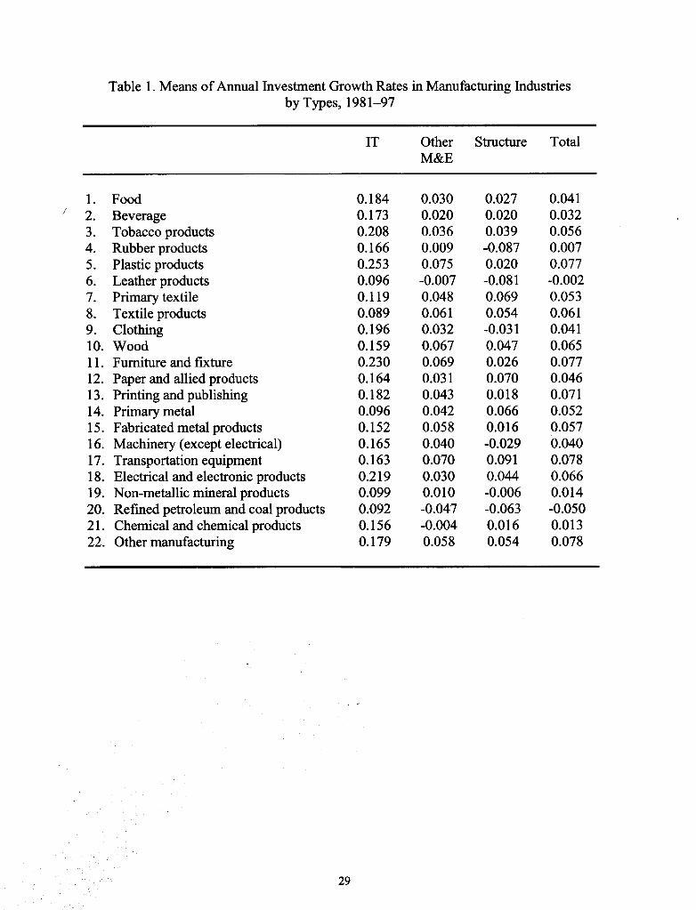
Table 1. Means of Annual Investment Growth Rates in Manufacturing Industriesby Types, 1981-97

IT Other Structure TotalM&E

1. Food 0.184 0.030 0.027 0.041I 2. Beverage 0.173 0.020 0.020 0.032

3. Tobacco products 0.208 0.036 0.039 0.0564. Rubber products 0.166 0.009 -0.087 0.0075. Plastic products 0.253 0.075 0.020 0.0776. Leather products 0.096 -0.007 -0.081 -0.0027. Primary textile 0.119 0.048 0.069 0.0538. Textile products 0.089 0.061 0.054 0.0619. Clothing 0.196 0.032 -0.031 0.04110. Wood 0.159 0.067 0.047 0.06511. Furniture and fixture 0.230 0.069 0.026 0.07712. Paper and allied products 0.164 0.031 0.070 0.04613. Printing and publishing 0.182 0.043 0.018 0.07114. Primary metal 0.096 0.042 0.066 0.05215. Fabricated metal products 0.152 0.058 0.016 0.05716. Machinery (except electrical) 0.165 0.040 -0.029 0.04017. Transportation equipment 0.163 0.070 0.091 0.07818. Electrical and electronic products 0.219 0.030 0.044 0.06619. Non-metallic mineral products 0.099 0.010 -0.006 0.01420. Refmed petroleum and coal products 0.092 -0.047 -0.063 -0.05021. Chemical and chemical products 0.156 -0.004 0.016 0.01322. Other manufacturing 0.179 0.058 0.054 0.078

29

Table 2. The Effects of Exchange Rates on Total Investment, 1981-97

~ ~ .QMM(1) (2) (3) (4) (5) (6)

L\el -0.2060 0.0380 -0.3215 -0.0566 -0.2336 0.1667

(0.268) (0.295) (0.318) (0.351) (0.328) (0.274)L\el-1 0.2399 -0.4454 -0.0338 -0.3104 0.1593 -0.5932

(0.241) (0.381) (0.266) (0.428) (0.293) (0.645)L\el-2 0.4400 0.4429 0.5642

(0.397) (0.426) (0.626)LL\el .0.0338 0.0326 -0.3552 0.0759 -0.0743 0.1377-J (0.273) (0.353) (0.352) (0.472) (0.458) (0.528)

L\uc -0.0683 -0.1142 -0.0520 -0.0711 -0.1074 -0.1553I

(0.041) (0.051) (0.050) (0.057) (0.052) (0.094).L\uc -0.0460 -0.1199 -0.0386 -0.0633 -0.0045 -0.1021

I-I

(0.044) (0.063) (0.054) (0.063) (0.044) (0.066)L\uc -0.0677 -0.0105 -0.0567

1-2(0.050) (0.056) (0.073)...

LL\ucl. -0.1143 -0.3019 -0.0906 -0.1448 -0.1119 -0.3142-J (0.068) (0.135) (0.082) (0.138) (0.080) (0.221)

.L\wm 0.1909 0.1230 0.0752 0.0828 0.1904 0.0956

I (0.194) (0.195) (0.125) (0.116) (0.100) (0.120)...

L\wm 0.2242 0.2069 0.2421 0.2047 0.2437 0.2440I-I (0.190) (0.192) (0.111) (0.142) (0.138) (0.179)

..L\wm 0.1605 0.3253 0.1922

1-2 (0.204) (0.159) (0.197)

LL\wm. 0.4151 0.4904 0.3174 0.6218 0.4340 0.5318I-J (0.279) (0.347) (0.162) (0.232) (0.154) (0.296)

Notes: Standard errors are in parentheses. Panel-corrected standard errors for OLS estimatesassume that disturbances are heteroscedastic and contemporaneously correlated across industries.Standard errors in 2SLS are corrected using White's (1980) procedure. All other explanatoryvariables are specified in equation (8). N= 308, except in column (1), where N= 330.* (**) Significant at the 10 (5) per cent confidence level.

30

Table 3. Measures of Volatility of Nominal C-6 Exchange Rate, 1981-97

P ta Coefficient of StandardY ehrcen gfe variation of deviation of GARCH Volatility

ear c ange 0 2 .3II I I monthly monthly (1,1) reglllle

annua eve 2 2level growth rates

1981 -0.87 -0.81377 -1.27685 -1.33105 Low

1982 -1.33 0.158801 1.278888 0.72354 High

1983 -2.396 -1.60868 -1.96799 -1.44364 Low

1984 4.1365 0.133328 -0.08409 -0.47069 Low

1985 4.9874 1.267762 -0.06336 -0.07817 Low

1986 5.5356 -1.23109 -0.98374 -1.00013 Low

1987 -3.905 -0.78157 0.517631 0.23599 Low

1988 -7.481 1.340967 1.101304 1.954785 High

1989 -5.789 -0.41281 -1.504 -0.61579 Low

1990 0.3338 -0.57422 1.274779 1.161185 High

1991 -0.864 -0.32459 -0.39724 -1.1799 Low

1992 7.1753 1.980801 -0.22039 0.907435 High

1993 7.0386 1.18266 0.689916 0.410561 High

1994 7.2075 0.51506 0.809002 0.630918 High

1995 1.4897 0.298468 1.035454 1.045659 High

1996 -1.319 -0.92141 -0.30898 -0.95535 Low

1997 0.8605 -0.20972 0.099656 0.004663 Low

1. A positive (negative) sign represents an exchange rate depreciation (appreciation).2. All three volatility measures are expressed in terms of the number of standard deviations away from thesample mean between 1991 and 1997. A positive (negative) sign represents that the volatility is above(below) the sample mean.3. Exchange rate movements are considered to be in the high-volatility regime if the fluctuations are morethan 0.5 standard deviation above the sample mean in at least two volatility measures.

31

Table 4. The Effects of Exchange Rates on Total Investment, 1981-97High- vs. Low-Volatility Regime

~ ~ QMM(1) (2) (3) (4) (5) (6)

0.2069 0.6320 0.2202 0.5786 0.1667 0.9468L\el (0.392) (0.410) (0.453) (0.485) (0.633) (0.588)

** ** **L\el-1 0.8643 0.6327 1.0398 0.8461 0.9410 0.8044

(0.360) (0.423) (0.437) (0.533) (0.395) (0.489)L\el-2 0.4111 0.4716 0.2812

(0.471) (0.581) (0.810)LL\el .1.0712** 1.6758** 1.2600** 1.8962** 1.1077* 2.0324**

-) (0.493) (0.551) (0.628) (0.744) (0.600) (0.678)

** ** ** **L\e xD~ -0.9008 -1.2713 -1.2223 -1.4170 -1.0448 -1.7393

I I

(0.565) (0.518) (0.619) (0.634) (0.682) (0.750)* ** ** ** * **L\e xD~ -1.002 -2.1315 -1.8439 -2.2585 -1.1652 -2.6503

1-1 1-1

(0.532) (0.683) (0.598) (0.816) (0.649) (0.883)L\e xD~ 0.1438 0.0096 0.34711-2 1-2 (0.450) (0.499) (0.571)

L(L\e .+L\e .XD~.) -0.8312* -1.5832** -1.8062** -1.7697** -1.1023 -2.0101**I-) I-) I-) (0.472) (0.694) (0.563) (0.815) (0.685) (0.785)

**L\uc -0.0474 -0.1049 -0.0200 -0.0587 -0.0566 -0.1244I (0.040) (0.051) (0.054) (0.059) (0.056) (0.090)

** **L\uc -0.0536 -0.1541 -0.0591 -0.1006 -0.0407 -0.15431-1 (0.043) (0.063) (0.058) (0.068) (0.041) (0.075)

**L\uc -0.1329 -0.0833 -0.1661*1-2 (0.056) (0.066) (0.089)

** *LL\uc .-0.1010 -0.3919 -0.0790 -0.2426 -0.0972 -0.4448

I-) (0.067) (0.140) (0.087) (0.149) (0.087) (0.236)

L\wm 0.2179 0.1489 0.1148 0.1096 0.1947 0.1529I (0.196) (0.186) (0.133) (0.123) (0.111) (0.128)

** *L\wm 0.2333 0.1733 0.2613 0.1732 0.2403 0.1601

1-1 (0.189) (0.183) (0.113) (0.131) (0.129) (0.185)*

L\wm 0.1328 0.2984 0.12171-2 (0.195) (0.154) (0.196)

** ** **LL\wm. 0.4512 0.4550 0.3760 0.5812 0.4350 0.4348

I-) (0.280) (0.330) (0.171) (0.224) (0.181) (0.321)

Notes: Standard errors are in parentheses. Panel-corrected standard errors for OLS estimates assume thatdisturbances are heteroscedastic and contemporaneously correlated across industries. Standard errors in 2SLSare corrected using White's (1980) procedure. All other explanatory variables are specified in equation (9). N =308, except in column (1), where N= 330. * (**) Significant at the 10 (5) per cent confidence level.

32

Table 5. The Effects of Exchange Rates on IT Investment, 1981-97

~ ~ Q:MM(1) (2) (3) (4) (5) (6)

~e 0.6116** 0.7952** 0.8217** 0.7910* 0.5922** 0.7995**I

(0.266) (0.217) (0.319) (0.418) (0.193) (0.387)~el-1 -0.3054 0.1314 -0.4380 0.1627 -0.3037 0.1467

(0.281) (0.302) (0.282) (0.410) (0.364) (0.428)** ** *~el-2 -1.0998 -1.1503 -0.9965

(0.376) (0.552) (0.552)L~el .0.3062 -0.1732 0.3837 -0.1967 0.2886 -0.0503

-J (0.263) (0.331) (0.331) (0.624) (0.347) (0.628)

**~uc -0.1408 -0.2585 -0.1222 -0.2270 -0.0664 -0.2106I (0.117) (0.132) (0.161) (0.175) (0.129) (0.186)

I~uc 0.1462 0.0268 -0.1035 -0.0122 0.1275 -0.34931-1 (0.101) (0.140) (0.149) (0.169) (0.112) (0.200)

~uc -0.0570 -0.0749 -0.11881-2 (0.080) (0.092) (0.096)*

L~uc. 0.0054 -0.2886 -0.2257 -0.3142 0.0612 -0.36431- J (0.152) (0.204) (0.158) (0.186) (0.177) (0.215)

~wm 0.1602 0.2124 0.1599 0.1742 0.2084 0.1149I (0.179) (0.170) (0.143) (0.145) (0.250) (0.215)

~wm -0.1617 0.0062 -0.1039 -0.0257 -0.1303 -0.06661-1 (0.173) (0.174) (0.195) (0.202) (0.197) (0.168)

~wm -0.0767 -0.0890 -0.06231-2 (0.182) (0.130) (0.153)

Notes: See notes to Table 2.

33

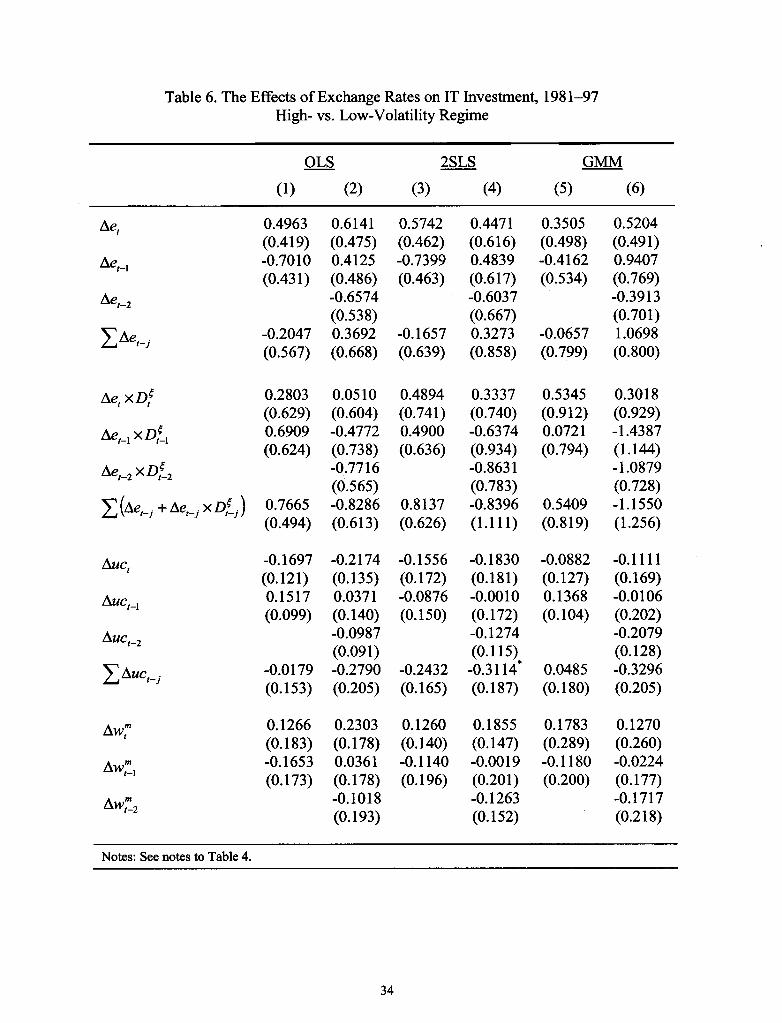
Table 6. The Effects of Exchange Rates on IT Investment, 1981-97High- vs. Low-Volatility Regime

~ ~ QMM(1) (2) (3) (4) (5) (6)

L\e 0.4963 0.6141 0.5742 0.4471 0.3505 0.5204I

(0.419) (0.475) (0.462) (0.616) (0.498) (0.491)L\el-1 -0.7010 0.4125 -0.7399 0.4839 -0.4162 0.9407

(0.431) (0.486) (0.463) (0.617) (0.534) (0.769)L\el-2 -0.6574 -0.6037 -0.3913

(0.538) (0.667) (0.701)LL\e 0 -0.2047 0.3692 -0.1657 0.3273 -0.0657 1.0698

I-} (0.567) (0.668) (0.639) (0.858) (0.799) (0.800)

L\e xD~ 0.2803 0.0510 0.4894 0.3337 0.5345 0.3018I I (0.629) (0.604) (0.741) (0.740) (0.912) (0.929)

L\e xD~ 0.6909 -0.4772 0.4900 -0.6374 0.0721 -1.4387I-I I-I(0.624) (0.738) (0.636) (0.934) (0.794) (1.144)

L\e xD~ -Q.7716 -0.8631 -1.08791-2 1-2 (0.565) (0.783) (0.728)

L(L\el-o +L\el_o XDI~o) 0.7665 -0.8286 0.8137 -0.8396 0.5409 -1.1550] ] } (0.494) (0.613) (0.626) (1.111) (0.819) (1.256)

L\uc -0.1697 -0.2174 -0.1556 -0.1830 -0.0882 -0.1111I (0.121) (0.135) (0.172) (0.181) (0.127) (0.169)

L\uc 0.1517 0.0371 -0.0876 -0.0010 0.1368 -0.0106I-I (0.099) (0.140) (0.150) (0.172) (0.104) (0.202)

L\uc -0.0987 -0.1274 -0.20791-2 (0.091) (0.115) (0.128)

*L L\uc 0 -0.0179 -0.2790 -0.2432 -0.3114 0.0485 -0.3296

I-} (0.153) (0.205) (0.165) (0.187) (0.180) (0.205)

L\wm 0.1266 0.2303 0.1260 0.1855 0.1783 0.1270I (0.183) (0.178) (0.140) (0.147) (0.289) (0.260)

L\wm -0.1653 0.0361 -0.1140 -0.0019 -0.1180 -0.0224I-I (0.173) (0.178) (0.196) (0.201) (0.200) (0.177)

L\wm -0.1018 -0.1263 -0.17171-2 (0.193) (0.152) (0.218)

Notes: See notes to Table 4.

34

Table 7. The Effects of Exchange Rates on Other M&E Investment, 1981-97

~ ~ QMM(1) (2) (3) (4) (5) (6).

~el -0.0513 0.3082 -0.5895 -0.0836 -0.2688 0.1847

(0.273) (0.273) (0.347) (0.369) (0.298) (0.192)~el-1 0.1330 -0.0377 -0.0463 0.0116 0.0083 -0.0824

(0.241) (0.296) (0.291) (0.413) (0.424) (0.388)~el-2 0.1680 0.1109 0.1271

(0.388) (0.513) (0.567).L~e, .0.0817 0.4385 -0.6358 0.0389 -0.2605 0.2294-J (0.242) (0.288) (0.353) (0.498) (0.458) (0.698)

.~uc -0.1042 -0.1475 -0.0661 -0.0500 -0.1467 -0.1142

I

(0.076) (0.086) (0.104) (0.110) (0.104) (0.189)~uc 0.0629 -0.0168 0.0185 0.0595 0.1105 0.0719

I-I

(0.081) (0.099) (0.096) (0.123) (0.102) (0.200)~uc 0.0124 0.1349 0.0874

1-2(0.083) (0.104) (0.171)

L~uc1. -0.0413 -0.1519 -0.0475 0.1445 -0.0362 0.0451-J (0.112) (0.197) (0.151) (0.261) (0.172) (0.542)

.~wm 0.1207 0.1113 0.1503 0.1900 0.1658 0.1632

I (0.190) (0.193) (0.118) (0.136) (0.097) (0.094)

~wm 0.1282 0.1525 0.2485 0.2555 0.2478 0.2340I-I (0.179) (0.196) (0.153) (0.177) (0.206) (0.233)

~wm 0.0476 0.2623 0.19131-2 (0.206) (0.237) (0.200)

Notes: See notes to Table 2.

35

Table 8. The Effects of Exchange Rates on Other M&E Investment, 1981-97High- vs. Low-Volatility Regime

~ ~ QMM(1) (2) (3) (4) (5) (6)

*~e 0.4089 0.8179 0.0835 0.4147 0.1409 0.7074I

(0.364) (0.429) (0.444) (0.513) (0.492) (0.584)~el-1 0.7865** 1.0539** 0.9447** 1.3445** 0.9995** 1.5098**

(0.296) (0.388) (0.416) (0.621) (0.404) (0.666~el-2 -0.0273 0.2305 -0.2140

(0.537) (0.660) (0.655)L~el-. 1.1953** 1.8445** 1.0282* 1.9897** 1.1404** 2.0031**

] (0.439) (0.516) (0.613) (0.803) (0.577) (0.935)

* * * ** *~e xD"" -1.0281 -1.0861 -1.4408 -1.3813 -1.347 -1.5868I I

(0.575l* (0.573) (0.784l* (0.796)* (0.648)* (0.821)*~e xD"" -1.1077 -1.9490 -1.6980 -2.334 -1.603 -2.541

I-I I-I

(0.436) (0.692) (0.617) (0.895) (0.655) (0.973)~e xD"" 0.3113 -0.2166 0.0018

1-2 1-2(0.476) (0.561) (0.774)L(~el-. +~el_.xD/~.) -0.9405** -0.8794 -2.1106** -1.942 * -1.810** -2.123 *

] ] ] (0.409) (0.576) (0.680) (0.892) (0.690) (0.927)

~uc -0.0376 -0.1116 0.0280 0.0018 0.0246 0.0073I (0.078) (0.093) (0.124) (0.129) (0.110) (0.220)

~uc 0.0727 0.0113 0.0347 0.0561 0.0785 0.1077I-I (0.073) (0.106) (0.097) (0.126) (0.098) (0.186)

~uc -0.0939 -0.0158 -0.09191-2 (0.095) (0.122) (0.200)

L~ucI .0.0351 -0.1943 0.0627 0.0421 0.1031 0.0230-J (0.105) (0.217) (0.164) (0.278) (0.190) (0.575)

* * * *~wm 0.1728 0.1792 0.2271 0.2711 0.2773 0.2984

I (0.196) (0.194) (0.127) (0.133) (0.136) (0.120)

~wm 0.1265 0.1274 0.2414 0.2483 0.2148 0.2369I-I (0.176) (0.194) (0.156) (0.174) (0.193) (0.233)

~wm -0.0238 0.1673 0.07321-2 (0.206) (0.228) (0.191)

Notes: See notes to Table 4.

36

Table 9. The Effects of Exchange Rates on Structure Investment, 1981-97

Q1s. ~ QMM(1) (2) (3) (4) (5) (6)

Ae -0.2469 -0.1099 -0.0670 -0.0511 0.1596 0.1337I

(0.358) (0.341) (0.479) (0.528) (0.581) (0.576)**

Ael-1 0.7153 -0.6104 0.2056 -0.5382 0.6041 -0.7662

(0.351) (0.490) (0.496) (0.728) (0.353) (0.671)Ael-2 0.4495 0.5521 0.2540

(0.453) (0.810) (0.690)LAel .0.4684 -0.2708 0.1386 -0.0372 0.7637 -0.3785

-J (0.413) (0.564) (0.532) (0.847) (0.584) (1.061)

** ** *Auc -0.0843 -0.1299 -0.0743 -0.0963 -0.0742 -0.1418

I (0.038) (0.044) (0.050) (0.062) (0.049) (0.074)** **

Auc -0.0620 -0.1541 -0.0512 -0.1091 -0.0486 -0.1653I-I (0.039) (0.051) (0.059) (0.072) (0.059) (0.076)

*Auc -0.0777 -0.0336 -0.1033

1-2 (0.044) (0.061) (0.068)** ** * **

LAucI .-0.1463 -0.3617 -0.1256 -0.2390 -0.1229 -0.4104-J (0.060) (0.111) (0.076) (0.155) (0.096) (0.201)

**Awm 0.3008 0.1504 -0.0145 -0.0701 0.3248 0.1704

I (0.249) (0.248) (0.257) (0.211) (0.158) (0.154)*

Awm 0.3778 0.3430 0.3523 0.2849 0.2658 0.3474I-I (0.235) (0.244) (0.195) (0.218) (0.182) (0.272)

*Awm 0.2092 0.4765 -0.1130

1-2 (0.243) (0.250) (0.290)

Notes: See notes to Table 2.

37

Table 10. The Effects of Exchange Rates on Structure Investment, 1981-97High- vs. Low-Volatility Regime

~ ~ QMM(1) (2) (3) (4) (5) (6)

L\e -0.1505 0.4757 0.1277 0.5708 0.3897 0.9411I

(0.583) (0.572) (0.780) (0.828) (0.930) (0.978)L\e 0.9103 -0.2621 1.379 0.0570 0.5756 -0.1527

1-1

(0.565) (0.616) (0.811) (0.899) (0.653) (0.812)L\e -0.0754 0.0263 -0.26991-2

(0.545) (1.087) (0.993)LL\e .0.7598 0.1382 1.5062 0.6542 0.9653 0.5185

I-J (0.786) (0.828) (1.108) (1.538) (1.144) (1.347)

L\e xD~ -0.2121 -0.8551 -0.5358 -0.9179 -0.4618 -1.6375I I (0.818) (0.722) (0.109) (1.104) (1.137) (1.118).

L\e xD~ -0.3378 -0.6168 -2.2899 -1.1817 0.1587 -1.30201-1 1-1 (0.816) (0.991) (1.226) (1.569) (1.009) (1.249)

L\e xD~ 0.8833 0.9449 0.85011-2 1-2 (0.606) (0.937) (0.975)

L (L\e,_. + L\e,- .x D! .) 0.2099 -0.4503 -1.3194 -0.5005 0.6623 -1.5709J J J (0.680) (1.050 (1.035) (1.359) (1.108) (1.597)

L\uc -0.0822 -0.1323 -0.0645 -0.1006 -0.0719 -0.1469I (0.038) (0.045) (0.055) (0.062) (0.056) (0.076)

L\uc -0.0639 -0.1605 -0.0673 -0.1222 -0.0538 -0.20191-1 (0.040) (0.053) (0.062) (0.075) (0.054) (0.081).

L\uc -0.0856 -0.0493 -0.15151-2 (0.052) (0.071) (0.084)

LL\uc .-0.1461 -0.3784 -0.1319 -0.272 -0.1257 -0.50031- J (0.061) (0.119) (0.077) (0.165) (0.103) (0.220)

..L\wm 0.3118 0.1684 0.0061 -0.0425 0.3147 0.2136

I (0.251) (0.244) (0.265) (0.209) (0.160) (0.164)

L\wm 0.3817 0.3171 0.3686 0.2535 0.2681 0.27661-1 (0.234) (0.243) (0.200) (0.215) (0.190) (0.296).

L\wm 0.2077 0.4520 -0.12061-2 (0.246) (0.249) (0.297)

Notes: See notes to Table 4.

38

Table 11. Classification of Industries

Average markup ratios

High Low

(HH) (LH)Primary textile Leather products

'fo Wood Primary metal

~ Paper and allied products Transportation equipment

~ Machinery (except electrical) Electrical and electronic products

[ Chemical and chemical products Other manufacturing~Q)

'i.b

~ (HL) (LL)Q)

~ Beverage Food~Q)

~ Tobacco products Rubber products

~ Plastic products Textile products~

Printing and publishing Clothing

Non-metallic mineral products Furniture and fIXture

Fabricated metal

39

Q)

:I"~

~~

O

N

~G

' >

~~

:>

~-

O'I\D

~

O'I

_M

~..d

§~~

N

~

f'!~

oo~

I:--:~

O\'~

p.o

m

--0- --

0,-"Q

) =

~

Q)

--,-- --,--

=Q

) ~

Q

)

E

.g:: e

Ii!:0

§0,d.9~

O

"~

oo~.5

Q)

=

,.., =

00 0'1--

0'1-- --

00--"Q

)~

~r-

--r- -.:I"

00 \D

or)

r- -.:I"

' ;:, , 0 ..p.

~

:>

N-.:I"

r-\D

3-.:1" ~

M

~~

~~

-~

~'-O

; '-O

;..;t; M

"'; r-..;t;

~Q

)~

'"'00

ON

.N

'-

'00,,;=0'1

,-- ,--

M--

---Q)u

Q)

S-~

Q)

~

Ii!:

~

~~

~.3

~

-.:I" "'s~

.,:j8

or)-- M

-- or)--

or)-- or)

~=

p.,..:I

r"- --r-

r- -or)

r- 0'1

-00 :

~

'" .,

.~'...I

:>

0'1 00

--0'1 0'1

0'1 or)

II'I::: Q

) ,;:, ~m

~

00

00 00

00 N

00

-00 --~

oS

Q

) '£

Om

~

--00 "":0

"":0 "":0

M

>~

a",

'"" c'd

,-- ,--

,-- 1--

--t'~

'" =

0 ~

~

08.~

~~

~

~

Q

) t=

.;:,

m

'"" =

I-.Q)~

~

Q)

oS>

~

0

0 ~

*

* -M

p.,..:I

~

p...;j

0\D

--0'1

--* --*

--or) 00

~

.~

-a ~

~

--r-r- O

M

--NO

'I :

0 Q

),,-;;,=,

.~

~

~

<5

'8 ~

ro

~

~

~

II II

~

,5 ~

~

:>

--0"": .0

0;0 0;0

N

;:;- 0~

.:Et

I-. ~

~

..,-, '"

~~

-~

=~

?<

?<

<I;

~

,.., ~

Q)

..., 00

.§(I)~

Q

) e.

~I-.

...~

>

- ~

-.,.' I-.

m

~

0 ,..,

~Q

) -.:1"--

or)-- 0--

00-- Q

»~

0>

C

' N

- -.:I"M

N

or) --.:I"

god ~

Ii'

~

0'100 \D

O

0'100 M

- 1-.00-

~-~

I:--:~

",;0;

~O

; I:--:~

,.!::::E

~

0

~

0- --00

OQ

)~,..:I

0 ,--

,-- ,--

,-- 00

oS

...,.m

0'1

o~-=

-'I

Q)

L. I'-" ,..,

Q)

L"" -.r:J

.~

~

-'" -..,'+

:1 "' ~

~

~

.S

'.6 ~

Q)

N--

N--

---or)-- :E

W

-",.,2co

--or) N

-M

00

~

,,'" =

C

:>

0'1-.:1" \D

or) or)-.:I"

0'10'1 ?':'

,",,~Q

)C

d 1

r- --.:I"

N

r- -.:I"

-.:I" 0

00 'l!

+

,S

g

O.

.' -.\D

. .,'..,

-.., Q

)0

,;:, '-"

~

~

~

~

---I --0

~ B

W

8.~

~

~~

"--

~o

c, ~

~

Q)u

0 ~

~

S

Ii!:=m

-I-.=

SO

Q)

,-, I-.

~

=

-U0

00-- -.:1"--

-.:1"-- M

-- r-

°..d~~

1-.Q

) C

"'- 0'100

-.:I"or) 000

_M

.Uu

cQ)

!:e j.;>

0

-r- \D

00 00

-.:I" -.:I" _II

~

~

~

Cd p.

~

~

f'!1:--: 1:--:1:--:

..;t;1:--: 0;1:--:

--OQ

):O=

p.o:;;-

--_0 -0

-0 N

O

M

t=-.r:J

~],-"

Q)

,-- ,--

,-- ,--

--Q)'+

:I -1-.0

E5

";II

~

] "E

~

e-

~

-a~oS

,Q

)N

0

=

,.., ..d

oS-r--

r- r-

.§ ,2

~

,~~

Q)

0-- --:

--: --r-

\D

"'~

"'e~

---00

r- --00

r- 0'1

Ir) ..oS

=

,.Q

:>

--or) r-

N

-M

-0 ,..,

Q)

Q)

,..:I ~

~

~

'8~

~"';

O~

or)l:--:

Jl- Jl-

~8

~~

:00

'- ~

O

1:--:0 N

-~

Q)

§ ",~

at --

-r:J

..., Q

) 00

'" ~

~

~

;:;::: t '£ 00

~0

~

'"',=

I-.

=,.-.,

"'0 Q

) ~

*

Q)

~

~

0*0

=

,;:, ,;:, '-"II

II 00

'" Q

) ~

*

~

~

,..:IQ)oS

o'~

~

~

~

~

oS

~

~

,~

.,.. 11

II II

II ~

~

§

? ~

~

~

~

~

~

~~

o8.~

-a.g~

~

~

~

~

~

~

~

z

e ~

:E

,S

40

Figure 1. Total Investment Growth in Manufacturing Sector, 1982-97

Real total investment Real GDP

15 ...,

/

/.

~~.c~e 0(9

\

-12

1982 1984 1986 1988 1990 1992 1994 1996

Figure 2. Real Investment Growth in Manufacturing Sector by Types, 1982-97

.c Total investment e IT.c

I Other M&E .Structures

~~.c~0'-(9

1982 1984 1986 1988 1990 1992 1994 1996

41

Figure 3. Real Investment Growth in Manufacturing Industries by Types, 1982-97

-~ ..'. -Total e IT

I, Other M&E e Structures

Food Beverage

0.96

~~~~-~'$ ~0 ~~ ;~;:#~ 9

-0.88

Tobacoo0.96

0

-0.88

1982 1997 7

Plastic Leather

0.96

0

-0.88

Prmary lextle TextI~ produc1s0.96

0 ~~~A~?

-0.88

7 1~ 1007

continued. ..

42

Figure 3. Investment Growth in Manufacturing Industries by Types, 1982-97(cont'd)

Total .IT( Other M&E .Structures

Cblhing Wood

0.96

Q

~.88

Furniture Peper

0.96

0

~.881~7 7

Printing Primary metal

0.96

0

~.88

F~ metel Machinery

0.96

Qr~~~~~.88

1~ 1~7 1982 1~7

continued. ..

43

Figure 3. Investment Growth in Manufacturing Industries by Types, 1982-97(concluded)

Total e ITi Other M&E ; ~ Structures

Transportation Electrical and electronic

0.96

0

.Q.88

7Non-metallic minerai

0.96

Q

.Q.88

1962 1~7

Refined petroleum and coal Chemical

0.96

0

.0.88

I'WI.-. ufactu .1962 1 ~7uu- man nrlg

0.96

0

.Q.88

1962 1991

44

Figure 4. Canadian Real Exchange Rates, 1981-97

.C-6 I Canada-U.S.

1.14085 .38444

cn:::J

~ cO

CJ -gcto

U

0.90725 .10166

1981 1983

45

Figure 5. Nominal C-6 Exchange Rates Volatility, 1981-97

C.V. in monthly level 1 --'rt---S..D. of monthly growth rates2

-+- GARCH (1,1)

~0:= 0cu .

"5G)

"U

"Ecu

"U~cu -0+' .

(/)

1/~

1981 v 7.ear

1. G.V. = coefficient of the variation2. S.D = standard deviation

46

Appendix A: The Effect of Exchange Rates on Marginal Benefits ofInvestment

As noted in the first-order conditions (3) and (4), for a given K, L, x and x* are optimally

chosen to maximize a firm's profit, depending on the domestic and foreign demand conditions, p

and p., and the price of the variable inputs, w. Thus, the marginal benefit of investment can be

expressed in the general form

a'l'/aK = h(K,p(e),ep.(e),w(e)). (AI)

Equation (AI) summarizes the key channels through which exchange rates affect the

marginal revenue product of capital. It is clear that p, p., and w are functions of the exchange

rate. Let us look at the corresponding changes in each of these components in the case of a

depreciation of the exchange rate; i.e., e increases. While the following discussion refers to a

depreciation, all considerations are simply reversed in the case of an appreciation. On the

domestic side, as imports become relatively more expensive in the domestic market, substitution

between imported and domestic goods raises the inverse demand, p. That is, the exchange rate

pass-through elasticity in domestic demand (If/ p.e) is positive. The elasticity of the marginal

revenue with respect to the exchange rate is:

~.::~ e = + A2a -(, , ~.-I 'I -I If/ p,e 'I+V-l e' ( )e P\l + v ) ,

where, -I = ~Q"'::~h-~~::il l .Since If/ > 0, equation (AI) states that, unless the domesticI+v ,e ae \1 + v- ) p,e

demand becomes less elastic such that, -I < -If/ p e , the marginal revenue from domestic salesI+v ,e ,

will increase as a result of the depreciation. Moreover, for a given level of K, an increase in the

marginal revenue causes the firm to produce more output, x + x., by raising L. For a

homogeneous production function, this higher level of L translates to an increase in the marginal

product of capital as K/L decreases. Hence, an increase (decrease) in the marginal revenue as a

result of a depreciation has a positive (negative) effect on investment.

On the foreign side, the primary effect is the direct valuation of the exchange rate on the

export price. A 1 per cent depreciation translates to a 1 per cent increase in the marginal revenue

47

due to the rise in export prices expressed in terms of the domestic currency. The firm may then

lower the foreign currency price of exports to capture a larger share of the foreign market. In a

monopolistic market, foreign fInns will respond by reducing their prices. This, in turn, will

generate some downward pressure on the inverse demand, p*. The exchange rate pass-through

elasticity in foreign demand ('1/, ) is negative. In terms of the exchange rate elasticity in thep ,e

marginal revenue of exports,

aep.(l +v.-I) e -I.):\ --.Ii .~,.-I \ -1 + \'1/, + ' I '-I , (A3)ue ep \1 + v ) p ,e +v ,e

where ' I '-I = ~h-:-~:;:j""i' In equation (A2), if the direct valuation effect dominates+v ,e ue \1 + v )

(i.e., '1/, +" > -1), the marginal revenue from foreign sales will increase when the currencyp ,e .u ,e

depreciates. Clarida (1997) finds that the effect of a depreciation on export revenue is

unambiguously positive regardless of the market structure. Similar to the domestic market, a rise

in marginal revenue from export sales also stimulates investment.

48

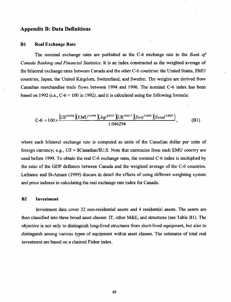
Appendix B: Data Definitions

Bl Real Exchange Rate

The nominal exchange rates are published as the C-6 exchange rate in the Bank of

Canada Banking and Financial Statistics. It is an index constructed as the weighted average of

the bilateral exchange rates between Canada and the other C-6 countries: the United States, EMU

countries, Japan, the United Kingdom, Switzerland, and Sweden. The weights are derived from

Canadian merchandise trade flows between 1994 and 1996. The nominal C-6 index has been

based on 1992 (i.e., C-6 = 100 in 1992), and it is calculated using the following formula:

(US 0.8584 XEMUO.0594 XJapO.0527 XUKO.0217 XSwitO.0043 XSwedO.OO35)C-6 = 100x, (HI)

1.046294

where each bilateral exchange rate is computed as units of the Canadian dollar per units of

foreign currency; e.g., US = $Canadian/$U.S. Note that currencies from each EMU country are

used before 1999. To obtain the real C-6 exchange rates, the nominal C-6 index is multiplied by

the ratio of the GDP deflators between Canada and the weighted average of the C-6 countries.

'- Lafrance and St-Amant (1999) discuss in detail the effects of using different weighting system

and price indexes in calculating the real exchange rate index for Canada.

B2 Investment

Investment data cover 22 non-residential assets and 4 residential assets. The assets are

then classified into three broad asset classes: IT, other M&E, and structures (see Table HI). The

objective is not only to distinguish long-lived structures from short-lived equipment, but also to

distinguish among various types of equipment within asset classes. The estimates of total real

investment are based on a chained Fisher index.

49

B3 User Cost of Capital

Taking taxes into consideration, the user cost of capital, UCiat, may be expressed as

follows for capital asset type a in industry i at period t (Christensen and Jorgenson 1969):

UC. = q . {( I-ViIZial -kiaI J[r +'l'. -(q;al -qial-I) ] +OJ. } (B2)lot 101-1 1- I 10 II ,

Vii qial-1

where q is the price of capital, a, and r is the interest payment if a loan is taken out to acquire the

asset. Alternatively, r can be interpreted as the opportunity cost of employing capital elsewhere

than in production. 'l' is the cost of depreciation or the loss in value of the machine as it ages.

The loss in value reflects the physical decay or loss of efficiency of the asset, and also the fact

that its expected service life has declined by one period. OJ is the effective rate of property taxes

( I-VZ-k )(nominal valued taxes assessed on the real stocks of land and structures), and is the

I-v

effective rate of taxation on capital income, where v is the corporate income tax rate, Z is the

present value of depreciation deductions for tax purposes on a dollar's investment in capital type

a over the lifetime of the investment, and k is the rate of the investment tax credit; (q:1 -qiat-l) is

qial-1

the expected capital gain.

50

Table Bl. Classification of Total Capital by Asset Classes

1. Infonnation Technology (IT)

.Computers & Office Equipment

.Communications Equipment

.Software-Own Account

.Software-Pre-Packaged

.Software-Custom Design

2. Other Machinery and Equipment (M&E)

.Office Furniture, Furnishing

.Household and Services Machinery and Equipment.Electrical Industrial Machinery and Equipment.Non-Electrical Industrial Machinery and Equipment.Industrial Containers.Conveyors & Industrial Trucks.Automobiles & Buses.Trucks (Excluding Industrial Trucks) & Trailers.Locomotives, Ships & Boats, & Major Replacement Parts.Aircraft, Aircraft Engines, & Other Major Replacement Parts.Other Equipment

3. Structures

.Non-Residential Building Construction

.Road, Highway, & Airport Runway Construction

.Gas & Oil Facility Construction

.Electric Power, Dams, & Irrigation Construction.Railway & Telecommunications Construction.Other Engineering Construction

.Cottages

.Mobiles

.Multiples

.Singles

51

Bank of Canada Working PapersDocuments de travail de la Banque du Canada

Working papers are generally published in the language of the author, with an abstract in both officiallanguages. Les documents de travail sont publiés généralement dans la langue utilisée par les auteurs; ils sontcependant précédés d’un résumé bilingue.

Copies and a complete list of working papers are available from:Pour obtenir des exemplaires et une liste complète des documents de travail, prière de s’adresser à :

Publications Distribution, Bank of Canada Diffusion des publications, Banque du Canada234 Wellington Street, Ottawa, Ontario K1A 0G9 234, rue Wellington, Ottawa (Ontario) K1A 0G9E-mail: publications@bankofcanada.ca Adresse électronique : publications@banqueducanada.caWeb site: http://www.bankofcanada.ca Site Web : http://www.banqueducanada.ca

20052005-21 The Effectiveness of Official Foreign Exchange Intervention in a

Small Open Economy: The Case of the Canadian Dollar R. Fatum and M.R. King

2005-20 La fonction de production et les données canadiennes P. Perrier

2005-19 Bank Failures and Bank Fundamentals: A Comparative Analysis ofLatin America and East Asia during the Nineties using Bank-Level Data M. Arena

2005-18 Lines of Credit and Consumption Smoothing: The Choice between Credit Cardsand Home Equity Lines of Credit S. Dey

2005-17 Risk Perceptions and Attitudes M. Misina

2005-16 Endogenous Central Bank Credibility in a Small Forward-LookingModel of the U.S. Economy R. Lalonde

2005-15 Learning-by-Doing or Habit Formation? H. Bouakez and T. Kano

2005-14 Labour Market Adjustments to Exchange Rate Fluctuations:Evidence from Canadian Manufacturing Industries D. Leung and T. Yuen

2005-13 Efficiency and Economies of Scale of Large Canadian Banks J. Allen and Y. Liu

2005-12 Do Exchange Rates Affect the Capital-Labour Ratio?Panel Evidence from Canadian Manufacturing Industries D. Leung and T. Yuen

2005-11 An Analysis of Closure Policy under AlternativeRegulatory Structures G. Caldwell

2005-10 Educational Spillovers: Does One Size Fit All? R. Baumann and R. Solomon

2005-9 State Dependence in Fundamentals and PreferencesExplains Risk-Aversion Puzzle F. Chabi-Yo, R. Garcia, and E. Renault

2005-8 Recent Developments in Self-Employment in Canada N. Kamhi and D. Leung

2005-7 Determinants of Borrowing Limits on Credit Cards S. Dey and G. Mumy

2005-6 Monetary Policy under Model and Data-Parameter Uncertainty G. Cateau

2005-5 Y a-t-il eu surinvestissement au Canada durant la seconde moitiédes années 1990? S. Martel