BANCO CENTRAL DE RESERVA DEL PERÚ

The Blessing of Natural Resources: Evidence from a Peruvian Gold Mine

Fernando M. Aragón * Juan Pablo Rud **

* Department of Economics, London School of Economics and Political Science

** Department of Economics, Royal Holloway, University of London

DT. N° 2009-015 Serie de Documentos de Trabajo

Working Paper series Diciembre 2009

Los puntos de vista expresados en este documento de trabajo corresponden a los de los autores y no reflejan necesariamente la posición del Banco Central de Reserva del Perú.

The views expressed in this paper are those of the authors and do not reflect necessarily the position of

the Central Reserve Bank of Peru.

The Blessing of Natural Resources:

Evidence from a Peruvian Gold Mine∗

Fernando M. Aragon† Juan Pablo Rud‡

November 2009

Abstract

This paper studies the impact of Yanacocha, a large gold minein Peru, on the local population. Using annual household data from1997 to 2006, we find robust evidence of a positive effect of the mine’sdemand of local inputs on real income. The effect, an average incomeincrease of 1.7% per 10% additional mine’s purchases, is only present inthe mine’s supply market and surrounding areas. We also find evidenceof improvements on measures of welfare and reduction of poverty. Weexamine and rule out that our results are driven by increased publicexpenditure associated to the mining revenue windfall. Using a spatialgeneral equilibrium model, we interpret these results as evidence ofnet welfare gains generated by the mine’s backward linkages and itsmultiplier effect.

Keywords: Natural resources, mining, local development.JEL classification: O13, O18, Q32, Q33, R20

∗We are particularly grateful to Tim Besley for his support and advice during this

research project. We also thank Nava Ashraf, Oriana Bandiera, Konrad Burchardi,

Francesco Caselli, Dave Donaldson, Claudio Ferraz, Greg Fischer, Maitreesh Ghatak,

Guy Michaels, Gerard Padro i Miquel, Torsten Persson and seminar participants at LSE,

Royal Holloway, the European Winter Meeting of the Econometric Society and Oxcarre

for useful comments and suggestions.†Department of Economics, London School of Economics and Political Science,

Houghton Street, London WC2A 2AE, United Kingdom; Tel: +44 (0)20 7852 3539; Fax:

+44-(0)20-7955-6951; Email: f.m.aragon@lse.ac.uk‡Department of Economics, Royal Holloway, University of London, Egham, Surrey,

TW20 0EX, United Kingdom; Tel: +44 (0)1784 27 6392; Email: juan.rud@rhul.ac.uk

1

The grudge against what has become known as the “enclave”type of development is due to this ability of primary productsfrom mines, wells, and plantations to slip out of a country with-out leaving much of a trace in the rest of the economy.

Hirschman (1958, p. 110)

1 Introduction

Access to natural resources has hardly been associated with development.A body of theoretical and empirical literature suggests that natural re-sources may not translate into better living standards or may even hin-der development (Sachs and Warner, 1999; Sachs and Warner, 2001; Caselliand Michaels, 2009). The current explanations for this “natural resourcecurse” focus on conflict, bad institutions, ineffective government or displace-ment of other productive sectors like in the Dutch disease (Benjamin etal., 1989; Torvik, 2002; Caselli, 2006). However, the available evidence tellus little about alternative channels such as the backward linkages betweenthe extractive industry and the rest of the economy, or the consequences atlocal level where many of the negative effects, such as pollution or populationdisplacement, occur.

In this paper, we fill this gap in the literature by investigating whethernatural resources benefit local communities and exploring the economicmechanisms for this to happen. We use the case of Yanacocha, a large goldmine in Peru, as a testing ground and evaluate the effect of the expansionof the mine on the income and welfare of the local population. In contrastto the existing literature, we focus on the general equilibrium effects of themine’s demand of local inputs as the main transmission channel.

In order to inform the way to look at the data, we first develop a spatialgeneral equilibrium model based on Fujita and Krugman (1995). In thissetup, there is a single city surrounded by a rural hinterland, specialized inthe production of manufactured goods and food, respectively. Both areasengage in costly intra-regional trade, and are also able to import goods fromother regions. The model treats the expansion of the mine as a demandshock on local labor in the city and delivers two testable predictions. First,if the mine expansion increases city’s real income, then the agricultural realincome also increases. The effect wanes the longest the distance to the mine’s

2

input market due to transportation costs. Second, there is an increase onthe relative price of locally produced food due to the relative larger demand.The increase on agricultural prices transmit the income gains to the ruralpopulation, not directly supplying goods or services to the mine.

We test these predictions using household data from repeated cross sec-tions. The data comes from household surveys - representative of the regionwhere the mine is located - for the period 1997 to 2006. We exploit twosources of variation to identify the effects of the mine expansion. First, weuse the significant increase on Yanacocha’s local purchases and wage billsince 2000. This phenomenon was driven by the increment on gold extrac-tion and the implementation of a corporate policy directed at increasinglocal procurement and employment. Second, we use the distance from thehousehold location to Cajamarca city - the mine’s local supplying market -as a source of heterogeneous exposure to the mine’s expansion.

We find a positive effect of the mine’s activities on real income in the cityand surrounding areas. The effect decreases monotonically with distanceand becomes insignificant beyond 100 km from the city. Our estimatessuggest that a 10 percent increase in the mine’s local purchases and wagebill is associated with an increase in real income of 1.7. We also observeincrements on the relative price of local food crops, such as potatoes andmaize. This is consistent with the effect on real income being driven by amarket mechanism and explains how the rural population benefitted fromthe demand shock in the city markets.

Nonetheless, in the presence of locational externalities associated to themine (such as pollution or crime), increments on real income do not implyan increase on welfare. Similarly, the average increase on income may hidenegative re-distributional effects, for example if poor households are unableto benefit from the mine expansion. To explore these questions, we firstfollow Roback (1982) who suggests using house prices as a measure of wel-fare.1 We find evidence of increments on house rental prices, in line withthe observed increase on real income, which we interpret as evidence of netwelfare gains due to the mine expansion. Second, we test for changes in self-reported measures of health and crime, but we do not find evidence thatthey have worsened with the expansion of the mine. Thirdly, we analyze there-distributional impacts of the mine expansion. Using quantile regressions,

1For an example of an empirical application, see Greenstone and Moretti (2003).

3

we find that the average household income at the bottom of the income dis-tribution has experienced an increase of real income similar to that observedfor richer households. We also find evidence of poverty reduction associatedto the mine expansion.

Finally, we investigate whether the observed phenomena is driven bythe revenue windfall to local governments or by the mine’s backward link-ages. This is a relevant question because of the importance attached to theincrement on public expenditure as one of the main benefits from naturalresource exploitation. We show that local public spending increases due tothe expansion of the mine. However, we find no evidence that this expansionof the public sector contributes to the observed increase in real income orwelfare.2 Instead, the observed phenomena seems to be driven entirely bythe expansion of the mine’s local purchases and employment. To the best ofour knowledge, there is not previous empirical work contrasting the relativeimportance of these two mechanisms.

In sum, our empirical results suggest that the expansion of the mineincreased real income and welfare of the local population. The effect seemsto be driven by the demand shock and its multiplier effect, associated tothe mine’s backward linkages not to the fiscal revenue windfall. The gainsare transmitted to residents in the rural area, not directly selling inputs tothe mine, due to the existence of trade within the economic region. Theincrease on the relative price of locally produced food crops is evidence ofthis transmission channel.

A main policy implication of our findings is that, even in the presence ofweak governments, natural resources can benefit local populations if back-ward linkages between the extractive industry and the rest of the economyare strong enough. However, as suggested by the model, this recommenda-tion hinges on the existence of economic integration in the regional economy(labor mobility and trade) as well as the pre-existence of good and labormarkets able to supply local inputs to the extractive industry.

The lessons to be drawn from this paper are not exclusive to extractiveindustries, they could apply to any business venture that creates a strongdemand shock in a relatively poor area. There are, however, at least two fea-tures that make large-scale mining a different and interesting case to study.

2Using the case of Brazil, Caselli and Michaels (2009) also find evidence suggesting thatthe oil revenue windfall to municipalities did not translate to increases on local income.

4

First, mining is a relevant industry for developing countries.3 According tothe World Bank, around 60 countries in the world have a mining sector largeenough, in terms of GDP or exports, to be a main driver of economic growthand poverty reduction (World Bank, 2002). However, understanding how totransform mining wealth into better living standards remains an unsolvedpolicy question. Second, there are well-documented negative local effectsassociated to mining. This increases the need to assess both direct and in-direct benefits on local communities to inform industrial and developmentpolicies.

This paper contributes to the literature studying the effect of naturalresources on economic development and to the literature examining howregional markets respond to demand shocks.4 Three features distinguish ourpaper from previous work. First, we use a microeconomic approach wherethe household is the unit of observation, as opposed to counties or districts.The comprehensiveness of the data allows us to explore in more detail themechanisms generating the spillover effects and to assess the net impact onresident’s welfare. Second, we show the importance of backward linkagesas a channel to improve local conditions. The mechanism we uncover hintsat an alternative explanation for the failure of natural resources to promotedevelopment: few linkages with local markets. This explanation relates toa technological feature of extractive industries and contrasts to the politicaleconomy argument used to explain the natural resource curse. Finally, we

3Developing countries play an important role in global mining. They are the largestproducers of key minerals like iron, copper and aluminium, and have almost three quartersof the world mineral resources. They account for most of the recent growth on miningproduction and attract an even increasing proportion of exploration spending (Humphreys,2009).

4There is not conclusive evidence of the effect of natural resources on development.Earlier studies use cross country data and find negative effects (Sachs and Warner, 1995;Sachs and Warner, 2001). However other papers using alternative measures of resourceabundance fail to find a negative relation (Lederman and Maloney, 2003; Sala-i-Martinet al., 2004). Using a microeconomic approach, Michaels (2006) finds that oil abundancein U.S. counties caused specialization, but that these costs were offset by populationgrowth and better education. In balance, oil-rich counties enjoyed higher income percapita without increase in inequality. Black et al. (2005) explore the effect of a coalboom in U.S. counties and find modest positive spillover effects on employment. Morerecently, Caselli and Michaels (2009) find no evidence of positive effect of oil extractionon income in Brazilian municipalities. In contrast, the literature on the impact of demandshocks (such as large industrial plants, construction works, casinos or military bases) findsome evidence of positive regional effects on wage bill and employment (Carrington, 1996;Hooker and Knetter, 2001; Evans and Topoleski, 2002), and resident’s welfare (Greenstoneand Moretti, 2003).

5

embed the study of natural resources (and local demand shocks) in theanalytical framework of a new economic geography model. This allows us toexplicitly explore general equilibrium effects and to introduce transportationcosts, agglomeration economies and migration which are relevant factorswhen studying a regional economy.

The remainder of the paper is organized as follows. Section 2 devel-ops the analytical framework we use to explore the effect of the mine on aregional economy. Section 3 presents background information about Yana-cocha and the relevant geographic area. Section 4 describes the data andidentification strategy. Section 5 presents the main empirical results relatedto the model predictions. Section 6 explores alternative explanations of theobserved phenomena. Section 7 presents robustness checks and section 8concludes.

2 Analytical framework

In this section we present a stylized model to shed light on the generalequilibrium effects of the expansion of a mine on a regional economy. Weuse the mono-centric city model developed by Fujita and Krugman (1995)and extend it by including an export sector and interregional trade. In thisframework, the mine is a foreign-owned net exporter that uses local laboras a production factor but sells all its output in international markets.5

We treat the expansion of the mine as a shock in the demand for locallabor and explore the effect on factor and good prices, and ultimately onreal income. The model allows us to analyze the spatial distribution of theeffects as well as the interaction of different economic sectors.

The model stresses the role of backward linkages, rather than alternativechannels such as forward linkages, agglomeration economies, public spendingor technology spillovers.

2.1 Environment

We consider a mono-centric spatial structure a la von Thunen, as depictedin Figure 1. In this spatial configuration, the regional economy is a longnarrow line with a single city surrounded by a rural hinterland that extends

5This setup resembles the characteristics of the mining activities of Yanacocha andother large modern mines.

6

from −f to f , where f represents the endogenously determined agriculturalfrontier. The land is of homogenous quality with one unit of land per unitof distance. Each location along the line is denoted by r. For simplicity, wedrop it when referring to the city (r = 0).

The economy has three productive sectors: manufacturing, agricultureand an export sector. The manufacturing sector produces a large number ofvarieties with an increasing returns to scale technology and has a monopo-listic competition structure. In contrast, the agricultural sector is perfectlycompetitive and produces a single homogeneous good, namely food. Theexport sector produces two goods: a manufactured commodity and the nat-ural resource, which are not consumed locally. Consumers in the region canimport consumption goods from other regions. Import and export goodsare homogenous and their prices are set in external markets.

All manufacturing, production of the export goods and import activitytakes place in the city, while the rural hinterland specializes in food produc-tion. We take this spatial system as given.6 There are (potentially) differentfactor and good prices in each location r, since we assume trade within theregion is costly. We use an iceberg transportation cost such that if 1 unitis transported over a distance d, only e−τd units arrive. The parameter τrepresents the transportation cost and is the same for all types of goods.7

The region has a given population of N workers who supply inelasticallyone unit of labor.8 Intra-regional migration is costless and workers canfreely move among locations. They live where they work, so we rule outthe possibility of commuting. The free mobility assumption implies that thepopulation allocation within the region is endogenous. In particular, thesize of the city L will depend on the spatial distribution of real wages.

Consumers All consumers share the same homothetic preferences U =XµAαM1−α−µ, where X is a composite index of the domestically produced

6Fujita and Krugman (1995) show that this configuration can be an equilibrium out-come, if some conditions are met. In particular, if the population is relatively small, ifmanufacturing goods represent a large enough proportion of consumers’ expenditure or ifconsumers have a sufficiently strong preference for varieties.

7The model predictions are similar if we assume different transportation costs for agri-cultural, manufactured and import goods.

8This assumption is very important since it precludes the possibility of inter-regionalmigration. However, the assumption is not a very strong one, if we take into accountevidence in the next section that shows very low levels of inter-regional migration flows inCajamarca over the analyzed period.

7

Figure 1: The monocentric economy

manufactured goods, A is the agricultural good or food and M is the importgood. The quantity index X is a CES function of the consumption of eachavailable variety:

X =(∫ v

0cρi di

) 1ρ

, 0 < ρ < 1,

where ci is the consumption of each individual variety and v is the range ofvarieties. The parameter ρ denoted the taste for variety and σ = 1

1−ρ , theelasticity of substitution between varieties.

The representative consumer’s budget constraint in location r is givenby

Y (r) = pa(r)A(r) + pm(r)M(r) +∫ v

0pi(r)ci(r)di,

where Y is the consumer’s income, pa is the price of food, pm is the price ofthe import good and pi is the price of variety i. Note that, due to transportcosts, prices and quantities are location-specific.

Consumers maximize their utility given the budget constraint. We cansolve the problem in two steps.9 First we minimize the cost of attaining Xand obtain the compensated demands for each variety ci(r) =

(pi(r)G(r)

)−σX

where G(r) =[∫ v

0 pi(r)1−σdi

] 11−σ is the price index for the manufacturing

composite. Then, we allocate the available budget between A, M and X

using the utility function parameters α and µ. The demand for the agricul-

tural and import goods are αY (r)pa(r)

and (1−α−µ)Y (r)pm(r)

respectively, while

the demand of the composite X is µY (r)G(r)

. Combining this expression with

the compensated demand we obtain the uncompensated demand for eachvariety:

ci(r) = µY (r)pi(r)−σ

G(r)−(σ−1). (1)

9For a detailed exposition see Fujita et al. (1999, pp. 46-48).

8

Furthermore, from the indirect utility function we can obtain the cost ofliving in a specific location r:

P (r) = G(r)µpa(r)αpm(r)1−α−µ. (2)

Manufacture producers The local manufacturing industry uses an in-creasing returns to scale technology with labor as the only production factor.In particular a firm requires li = F + βxi units of labor to produce xi unitsof a variety of the manufacturing good. The presence of increasing returnsto scale implies that each variety is produced by a single firm. There is freeentry and exit to the industry, hence in equilibrium manufacturing firmsmake zero profits.

A firm’s profit is equal to pixi − wli, where xi = ci as in equation (1)and w is the wage in the city.10 The resulting profit-maximization price is

pi =σ

σ − 1βw. (3)

Note that this result implies pi = p, i.e. all varieties have the sameprice, since they all share the same marginal cost β. It follows that themanufacturing price index becomes G = pv

11−σ and the location-specific

individual demand for each variety (1) as

c(r) =µY (r)p(r)v

. (4)

From the zero-profit condition we obtain a firm’s individual supply x =F (σ − 1)

βand its labor demand l = Fσ.

Agricultural production and rural hinterland Farming uses a fixedproportion technology. It requires 1 unit of land and ca units of labor toproduce 1 unit of food. Food is consumed locally and the surplus, a propor-tion 1−α, is sold to the city.11Landlords live in their landholdings, hence allthe agricultural income is consumed locally. For a given frontier f the totaldemand of labor from the agricultural sector is 2caf and total food supplyto the city is 2 (1− α)

∫ f0 e−τrd

10In the city, given the manufacturing sector zero-profit condition, the wage w is alsothe average income.

11This follows from the representative consumer’s maximizing food consumption.

9

Food is traded in the city at a price pa. However due to transportationcosts, the price of food received by farmers decreases with distance to thecity, i.e. a farmer in location r receives pa(r) = pa e

−τ |r| where |r| measuresthe distance to the city. This means that the opportunity cost of consumingfood is lower the greater the distance to the city.

In contrast, since the manufactured goods and import need to be shippedfrom the city to rural areas for their consumption, the corresponding pricesincrease with distance. In particular, in location r the price of the manufac-ture composite is G(r) = Geτ |r| and the price of imports, pm(r) = pme

τ |r|.Taken together, these results imply that the price index in location r is

P (r) = Pe(1−2α)τ |r|. (5)

Under the assumption that locally produced food represents less than halfof a household’s expenditure (α < 0.5), the cost of living increases withdistance.12

Since landlords use ca units of labor to produce 1 unit of food, theirrents are R(r) = pa e

−τ |r| − caw(r), where w(r) is the wage rate in locationr. The hinterland extends around the city up to the point where rents are

zero, or w(f) =pae−τf

ca. Costless migration implies that in equilibrium the

real wage is the same in all locations. In particular we compare the realwage in the city and in the agricultural frontier to obtain the following wageequalization condition13:

w =pae−2(1−α)τf

ca. (6)

Finally, we derive total demand for manufactures and import goods fromthe rural hinterland. Note that a proportion µ of the local income is con-sumed in the manufactured good while the remaining 1 − α − µ is spenton imports. In the rural hinterland, the total income -distributed betweenlandlord and workers- corresponds to the price of the agricultural outputpa(r). Since landlords and agricultural workers share the same homothetic

12We require farmers to trade a significant part of their production. It does not meanthat the consumption basket of rural farmers is not mainly food, since many of the im-ported goods can be foodstuff produced elsewhere. Results do not hinge on this assump-tion.

13Real wage equalization and the price index defined in (5), give us a nominal wage inlocation r equal to w(r) = we(1−2α)τ |r|.

10

preferences, we can treat their demand as the one of a representative con-sumer. Replacing the values of local prices and income, we obtain the totaldemand of each manufactured good variety and import goods from the ruralhinterland:

Manufactured goods: 2µpapv

∫ f

0e−2τrdr (7)

Imported goods: 2(1− α− µ)papm

∫ f

0e−2τrdr. (8)

Export sector There are two types of firms in the export sector: produc-ers of a tradeable commodity and a mine that extracts the natural resource.Both use labor as their input and sell their output in perfectly competitiveexternal markets.

In contrast to the manufacturers supplying the domestic market, thecommodity producers face decreasing returns to scale. In particular, theirproduction function is E (Le) = Lεe, where E is the amount produced ofthe commodity, Le is the size of the workforce employed in the industryand ε < 1. The industry profit is peE (Le) − wLe, where pe is the price ofthe commodity. Solving for the profit maximization problem we obtain theunconditional labor demand function:

Labor demand: Le (w) =(εpew

) 11−ε

. (9)

Note that εpeE is paid, as wages, to local workers; while the industryprofits πe = (1− ε) peE are distributed among the firms’ shareholders. Forsimplicity we assume that all shareholders reside in the city and have similarpreferences than workers.

The mine uses a fixed proportion of local labor in its production process.The demand of local labor is θS, where S is the mine’s production and θ < 1is exogenously determined. Note that θ captures the extent of backwardlinkages between the mine and the local economy. The mine is foreign-owned and there are no taxes, hence all the profits are remitted abroad.

2.2 Equilibrium

The instantaneous equilibrium is given by the solution of the following sys-tem of non-linear equations:

11

F (σ − 1)β

=µ

pv

(Lw + 2pa

∫ f

0e−2τrdr + πe

)(10)

2 (1− α)∫ f

0e−τrdr =

α

pa(Lw + πe) (11)

L = vFσ + Le (w) + θS (12)

w =pae−2(1−α)τf

ca(13)

peE(w) + wθS = (1− α− µ)(Lw + 2pa

∫ f

0e−2τrdr + πe

)(14)

p = βwσ

σ − 1(15)

N = L+ 2caf. (16)

Equation (10) represents the market equilibrium of each variety of thelocal manufacture. The total demand on the right hand side is proportionalto the regional income which is composed by the wages paid to city work-ers, agricultural income and the profits from the commodity export firms.Equation (11) is the food market equilibrium condition while equation (12)represents the equilibrium in the city’s labor market. Note that the labordemand in the city comes from local manufacturers, commodity export firmsand the mine.

Equation (13) is the wage equalization condition (6) obtained from theassumption of costless migration. Equation (14) represents the current ac-count’s balance: in equilibrium the value of exports minus the net factorpayments should be the same as the value of total imports.14 Equation(15) is the manufacturers’ profit maximization condition (3). Finally, equa-tion (16) represents the population constraint, where the size of the regionalpopulation equals the number of workers in the city and in the agriculturalsector.

We solve the system analytically. First note that, using (12) and (16),we can write the number of manufacturing firms, v, as:

v(w, f) =N − 2caf − Le (w)− θS

Fσ. (17)

14We assume a fixed exchange rate equal to 1.

12

Using this result, replacing (14) into (10) and re-arranging, we obtain:

N − 2caf −(1− α− µ) ε+ µ

(1− α− µ) εLe(w)− 1− α

1− α− µθS = 0. (AA)

Note that expression (AA) defines an upward sloping curve in the space(f, w). This curve has a positive intercept and also an upper bound f onthe values that f can adopt.15

Second, using (9), (13) and (16), solving for the integral over f andrearranging, we can rewrite the equilibrium condition in the food market(11) as:

2ca[(1− α)(1− e−τf )αe−2(1−α)τf

+ f ]−N − (1− ε)ε

Le(w) = 0. (BB)

This expression defines a downward sloping curve in the space (f, w), witha lower bound f on the values of f .16

Intuitively, the curve AA is upward sloping because with a larger ruralhinterland (higher f), the city has a smaller population and hence the laborsupply is smaller. This translates into higher wages in the city. In contrast,curve BB is downward sloping because higher wages in the city increaseagricultural wages (due to costless intra-regional migration). In turn, thismeans that the marginal farmer makes losses and hence the agriculturalfrontier shrinks (smaller f).

To solve the model we plot curves AA and BB (see Figure 2). Theintersection of both curves at point Q provides the unique pair (f∗, w∗) thatsolves the system and defines the equilibrium.17

2.3 The Effects of the Mine’s Expansion

We are now ready to use the model to perform a thought experiment andanalyze the effect of the mine’s expansion on the regional economy.

We simulate the expansion of the mine as an increase on S, the amount of

15To see this, note that f ≡ limw→∞

f = 12ca

(N − 1−α

1−α−µθS)

and that limf→0

w =

L−1e

(2caf

(1−α−µ)ε+µ(1−α−µ)ε

), where L−1

e is the inverse function of Le(w).16Note that f≡ lim

w→∞f = g−1 (N), where g−1 (·) is the inverse function of g(f) ≡

2ca[ (1−α)(1−e−τf )

αe−2(1−α)τf + f ].17See Appendix A.1 for a formal proof.

13

Figure 2: Model equilibrium

natural resources extracted by the mine. The immediate effect of this shockis to increase demand of labor and shift the curve AA upwards as depictedin Figure 3. To understand this shift note that f defines the distributionof people between city and rural countryside, and thus the labor supply ineach area. Hence, keeping the labor supply fixed, increments on the demandfor labor in the city due to the mine expansion would increase local wages.

As we see in Figure 3, the equilibrium moves from point Q to Q′ with ahigher wage in the city but smaller f . The reduction on f implies a smallerextension of agricultural frontier and a larger city population. Since N isassumed to be fixed, the grow of the city requires migration of agriculturalworkers to the city.18 In this model, the increase on wages - triggered bythe mine expansion - is partially offset by migration to the city.

Crowding out The expansion of the mine, and the subsequent wage in-crement, displaces other economic activities. First, the reduction on theagricultural frontier implies a smaller agricultural production. Second, thehigher wage reduces the employment, output and profits of the export sec-

18The assumption of a fixed N is important to obtain the model predictions. If weassume instead costless inter-regional migration, the effect of the mine expansion on realincome would be zero.

14

Figure 3: The expansion of the mine

tor which uses labor as its only production factor. This result is similar inflavor to the “Dutch disease”, commonly found in macroeconomic models ofresource boom (Corden and Neary, 1982). In this case, the crowding out isdriven by increase on the relative price of a production factor.

Nonetheless, the effect on the local manufacturing industry could be ei-ther positive or negative. On the one hand, the growth of the city populationfavors the increase on the number of firms, v, due to the increasing returns toscale. On the other hand, this positive effect is offset by the expansion of themine’s labor demand, which reduces the labor available for manufacturingfirms. The net effect depends on the extent of the mine’s backward link-ages, θ. In particular, if it is sufficiently high, v would increase, because themultiplier effect would make the city population grow enough to satisfy theadditional labor demand from the mine without harming the manufacturingindustry.19

19See Appendix A.2 for a formal derivation of the condition.

15

Effect on real wages From (2), we can obtain an expression for the realwage in the city:

ω =w

P=(wG

)µ( wpa

)α( w

pm

)1−α−µ, (18)

where G = pv1

1−σ and σ > 1.Note that the wage relative to the price of food and import goods ( wpa

and wpm

) increases as a consequence of the expansion of the mine.20 Theseresults highlights two sources for real wages to increase: the increase on thepayments to labor relative to land rents, due to the additional demand; andthe access to relatively cheaper import goods. However, the effect on realwages is ambiguous, because these gains may be offset by higher price ofmanufactured goods (G), if the number of firms reduces.21

2.4 Testable predictions

The previous results provide the basis for the two testable predictions of themodel regarding the effect of the mine expansion on real income and relativeprices.

2.4.1 Effect on real income

The income in the city and rural hinterland comes from different sources.In the city, the income is composed by wages and the dividends from exportfirms. In contrast, in the rural hinterland it is proportional to the value ofthe agricultural output pa(r). Taking that into account, we can write theaverage real income in location r as:

y(r) =

{ω + πe

PL if r = 01kpaP e−2(1−α)τ |r| if r 6= 0,

(19)

20To see this note, from (13), that wpa

is decreasing on f and hence increases withS. Additionally, given that the price of imports pm is exogenously determined and wincreases, w

pmalso increases.

21We can, however, identify two plausible cases in which the real wage increases: whenv increases, and when v decreases but local manufactures represent a small proportion ofthe budget (small µ). See Appendix A.3 for a formal derivation of these conditions.

16

where y(r) is the average real income, P is the general price index in the city,and k is the unknown, but constant, population size in each rural locality.22

The effect of the mine expansion on the income of city residents is, apriori, unclear and remains an empirical question. On the one hand, itincreases due to higher wages. On the other hand, it decreases due toreduction on the profit of export firms, crowded out by the mining sector,and the (potential) increase on the price of the manufactured good due tothe smaller number of firms.

We focus on the case in which the real income in the city increases withthe mine expansion. In this case, the model provides clear testable predic-tions regarding the relation between income in the city and rural hinterlandand relative prices.

Proposition 1 If the real income of city residents increases, then the realincome of rural inhabitants must also increase.

Intuitively, the growth of urban income combined with the larger citypopulation increases the demand for food. This demand shift, combinedwith the reduction on food supply due to the smaller agricultural frontier,necessarily results on an increase in the price of food and on higher incomein rural locations.

To explore the effects on welfare, note that the indirect utility of a house-hold in location r is V (r) = µµαα(1 − µ − α)1−µ−αy(r). Hence, the realincome becomes a sufficient statistic for welfare, however this result doesnot hold in presence of externalities from the mine. For that reason, in theempirical section we explore different measures of welfare in addition to realincome.

In this model, the shock of demand created by the mine expansion di-rectly affects the city’s labor and goods markets. The effect is transmittedto the surrounding rural areas due to the trade links between the city andits rural hinterland. Since intra-regional trade is limited by the existenceof transportation costs, a relevant question is how the effects of the mineexpansion are distributed spatially in the economic region.

Proposition 2 When the mine expansion increases real income, the effectdecreases monotonically with distance to the city.

22Recall that in each farm there are ca workers and a landlord, but it does not correspondto the total population since a landlord can also be a worker.

17

The model predicts heterogeneous effects by distance, because trans-portation costs reduce the land rents for farmers in farther locations andabsorb part of the gains on real income. In the extreme, beyond the agri-cultural frontier, the effect is nil since there is no trade with the city. Inthe empirical section, we use this insight as a key element of the identifica-tion strategy. In particular, we obtain the distance from a locality to thecity, and use it as a measure of different exposure of households to the mineexpansion.

2.4.2 Effect on relative prices

The increase of real income, and its transmission to agents not directlyemployed by the mine, are driven by changes in the relative prices of laborand food. To explore this mechanism further, we use the model to obtainpredictions regarding the effect of the mine expansion on relative priceswithin the economic region. We focus on two types of goods that are possibleto identify in the data: the agricultural good and the import good.

Proposition 3 If the real income of city residents increases due to the mineexpansion, then pa(r)

P (r) also increases. The effect on pm(r)P (r) is ambiguous.

The relative price of food in the region increases because it is proportionalto the real agricultural income. In contrast, the effect on the relative priceof the import good is ambiguous since G, one of the components of the priceindex may increase or decrease. However, if local manufactures representa small proportion of the consumption basket, then the relative price ofimports would actually decrease due to the increase on price of food. Acorollary of this result is:

Proposition 4 if the real income of city residents increases due to the mineexpansion, then the increase on y(r) is greater than the increase on Y (r)

pa(r),

where Y (r) is the nominal income in location r.

Note that Y (r)pa(r)

= y(r)pa(r)/P (r) . It is straightforward to see that the change

on Y (r)pa(r)

is smaller than the change on y(r) since pa(r)P (r) also increases due to

the mine expansion.This result sheds light on the transmission channel of the effect from the

city to the rural hinterland. Since rural income increments are driven for

18

higher food prices, the income relative to the price of food should not varyas consequence of the mine expansion. In the city, the increment may bepositive, but still smaller than the increase on y.

3 The Case of Yanacocha Gold Mine

Peru has a long tradition as a mining country and ranks among the topproducers of minerals in the world.23 In the late 1990s it experienced amining boom and the sector expanded significantly. In the relevant periodfor our analysis, from 1997 to 2006, the mining product grew at an averageannual rate of 7.4% while the economy growth rate was around 3.5%. As aconsequence, the share of the mining sector in GDP went from 3.8% to 5.2%(Banco Central de Reserva del Peru, 2009). The mining growth has beenmostly driven by the opening and expansion of large mining operations ingold, copper and silver.24

One of the largest new mines is Yanacocha. The mine is privately ownedand none of the investors resides in the locality.25 Yanacocha is the secondlargest gold mine in the world, representing around 45% of the total Peruviangold production, and the most profitable. The mine extracts gold from openpits and uses a very capital intensive technology. All production is exportedas gold bars, with no other processing or added value. This feature precludesthe creation of forward linkages.

The mine is located in the department of Cajamarca in the North High-lands of Peru. The department of Cajamarca is mostly rural and relativelypoor. In 2006, Cajamarca was the eighth department (among 24) in terms ofincidence of poverty, with 63.8% of the population living below the povertyline (INEI, 2007). The mine is located less than 50 km. away from Ca-jamarca city, the department’s capital and largest urban settlement (seeFigure 4 for a map of the spatial configuration). Due to the proximity tothe city, most workers and local suppliers live there. This feature facilitates

23In 2006 it was the first producer of gold, zinc, silver, lead and tin in Latin Americaand among the top five producers of those minerals in the world (Ministerio de Energıa yMinas, 2006).

24Some of the new mines are Yanacocha (gold), Pierina (gold) and Antamina (silverand copper).

25The mine shareholders are: Newmont Mining Co., with more than 50% of the shares,Compania de Minas Buenaventura (more than 40% of the shares) and the World Bank(around 5% of the shares). Newmont Mining Co. is a U.S. based company, while Companiade Minas Buenaventura has its headquarters in Lima, Peru’s capital city.

19

our analysis, because the city becomes the geographical market where themine purchases local goods and services.26 There are other three majorcities in the surroundings (Trujillo, Chiclayo and Chachapoyas) and somesmall and medium mines in the south of Cajamarca.27

3.1 Mine Production and Local Procurement

Yanacocha started operations in 1993, and its production increased steadilyover time. In 2001, it expanded its production due to the opening of newgold deposits Figure 5 shows the expansion of the mine production since1997 and the change of trend since 2001 associated to the expansion of theproduction capacity.

The growth on the mine size has required a steady increase on the pur-chase of production inputs such as explosives, machinery, oil, laboratoryservices, limestone, etc. As we will see below, the mine expansion coupledwith a shift in procurement policies has increased Yanacocha’s local pur-chases and employment.

Yanacocha procures its inputs in three ways: purchasing goods to suppli-ers, directly hiring workers and contracting out services. In terms of origin,Yanacocha classifies the supplying firms as local and non-local dependingof where they are registered for tax purposes and the origin of their share-holders.28 In particular, for a firm to be considered local it has to pay taxesin Cajamarca and have at least 50% of Cajamarquinos among their share-holders. For individuals, the requirement is to be born in Cajamarca or todemonstrate continuous residence for at least five years in Cajamarca.29

In the first years of operation, Yanacocha had little economic interactionwith the city of Cajamarca and its surroundings, with only a very smallproportion of inputs bought locally (Kuramoto, 1999). For example, in1998 the value of purchases from Cajamarca represented 3% of total goodpurchases and 15.5% of services. In contrast, purchases from Lima were77.5% and 72.6% of goods and services respectively. The rest was bought

26Yanacocha classifies its purchases by origin as local (sourced in Cajamarca), national(bought from the rest of the country, mostly Lima) and foreign.

27These mines use more traditional technologies, have smaller scale and are more laborintensive than Yanacocha.

28The non-local category includes Lima, rest of Peru, and other countries.29This information was obtained from internal memorandums and interviews with Yana-

cocha representatives.

20

Figure 4: Location of mine and main cities

21

abroad or in the rest of the country. There were also very few local firmsamong the top mine suppliers.30

A shift in procurement policy Since late 1990s, the mine started ashift in its procurement and employment policies aimed to increase the par-ticipation of local firms and workers. The policy change was promoted bythe International Finance Corporation, one of Yanacocha’s shareholders andNewmont’s main lender, as a way to increase the economic impact of themine in the region and minimize the risk of conflict with the local population(Jenkins et al., n.d.).31

The most important feature of the mine procurement policy was to givepriority to local suppliers and workers in competitive bids and recruitment.32

For example, a 2006 policy memorandum by the mine aiming at outsourc-ing services such as cleaning, waste management or transport, establishesthat “in competitive bids with non-local companies, the Company has toprioritize the hiring of Cajamarquino small and medium enterprizes”. Sim-ilarly, the memorandum specifies that the mine should ensure that at least60% of personnel of the mine contractors reside in Cajamarca. This shift inpolicy becomes apparent in the evolution of local purchases and wage bill(including bonuses) that show a significant increase since 2000 (see Figure5).

What does the mine buy locally? The local purchases consist of rel-atively simple services and goods, with low quality requirements and notconsidered vital to the mine operations. The expenditure on services islarger that the expenditure on goods.33 The main local services contractedlocally include demolition, haulage and transport of material to leach pads,and cleaning and reforestation activities. More specialized services such astransport of dangerous materials, consulting, engineering, laboratory anal-ysis, etc., are supplied by firms located in Lima or abroad. In the case

30Among the top 20 suppliers, there was only one local firm. In the case of serviceproviders, there were four local firms among the top contractors.

31IFC is promoting policies to increase supply chain linkages in other mining, oil and gasprojects. For example, a similar approach is being development in a new mine operatedby Newmont in Ghana.

32Yanacocha has also promoted quality certification among its suppliers, but it has notengaged in direct transfer of technology or training.

33For example, in 2004 the expenditure on services was around nine times greater thanthe expenditure on goods.

22

Figure 5: Evolution of Yanacocha’s local procurement and production

of goods, local purchases consists mostly of construction materials, basichardware, cleaning materials, vehicles spare parts chemical products, officefurniture, etc.

Even though local purchases and wages would imply different channelsthrough which the activity of the mine affects household incomes (e.g. directeffect of wages or development of backward linkages), the distinction is not asclear-cut as it seems. The mine hires some workers directly; however, mostworkers located in the mine site are employed by contractors who provideservices to the mine.

Figure 6 shows the evolution of the number of workers in the mine,directly employed by Yanacocha or indirectly through contractors. In theperiod 1997-2006 the number of total workers increases from 4,000 to 14,000,a substantial proportion of the active population of Cajamarca. To putthis numbers in context, the mine’s workforce represented around 12% ofthe active population of the city of Cajamarca in 2001 and 20% in 2005.Consistent with the mine policies, 60% of the workers are locals and almostall of them live in Cajamarca (Minera Yanacocha, 2006)

23

The increase of mine employment occurred in 2000 and was drivenmainly by workers indirectly hired through contractors. Contractor workersrepresent a significant proportion of the mine’s workforce. In average theyrepresent 78.5% of the total mine workers. Workers that are hired directlyby Yanacocha, tend to be skilled (engineers, accountants, technicians, sec-retaries, assistants, supervisors) as opposed to low-skilled workers employedthrough contractors.

Figure 6: Direct and indirect employment

4 Data and identification strategy

4.1 Data and main variables

Household data The empirical analysis uses data from repeated crosssections of the Peruvian Living Standards Survey, an annual household sur-vey collected by the the National Statistics Office (INEI).34

The survey consists of a stratified household sample representative at34The name of the survey is Encuesta Nacional de Hogares or ENAHO.

24

regional level. The regions are defined for statistical purposes and considerboth environmental conditions (coast, highlands and forest) and geographi-cal location (north, center and south).35 We focus on the North Highlandsstatistical region, where the mine is located. The data set covers 10 years,between 1997 and 2006, and includes more than 7700 households.36

Figure 7 shows the area of study and the spatial distribution of thesample. The area covers a surface of almost 40,000 square kilometers andhad an estimated population of 1.2 million inhabitants in 2005.37 The darkershaded areas correspond to districts sampled at least one year, while lightershaded ones are districts for which there are not available observations. Wecan see that the sample is evenly distributed over the area of study.

The main purpose of the survey is to measure poverty and living stan-dards. The survey contains detailed information on income, expenditure,socio-demographics (such as gender, age, educational attainment of indi-viduals), composition of the household, housing characteristics like accessto public utilities and construction materials, and self-reported incidence ofhealth problems and exposure to crime. The data set also has extensiveinformation on prices and agricultural activity at household level.

Additionally, we obtain the distance from the household’s location to thecity. We measure distance as the length of the shortest path between themain town of the household’s district and Cajamarca city using the existingroad network. We performed the calculation using the ArcGIS softwareand maps produced by the Ministry of Transport of Peru. The road mapcorresponds to the network available in 2001 and includes only tracks usableby motorized vehicles. In terms of the model, this variable is the empiricalcounterpart of r and relates to the total transportation cost from one locationto the city markets. As suggested by the model, the effect of the mineexpansion should decrease with distance to the mine’s supplying market.As describe below, we and exploit this heterogenous effects by distance toidentify the effect of the mine on the regional economy.

Table 1 shows the estimated mean of the main variables at household35In general, these statistical regions are larger than departments and do not necessarily

share the same boundaries.36In line with the model, we restrict attention only to household with an employed

household head. This filter reduces the sample by just 46 observations and does not affectthe results.

37The population estimates are obtained from the ENAHO survey.

25

Figure 7: Area of study and spatial distribution of sample

26

level. Since we are using an stratified sample, the means are estimated usingsampling weights. In the second column we report the standard errors of themean estimates, which are calculated using sampling weights and clusteringby primary sampling unit.

Table 1: Mean of main variables at household level

Variables Mean StandardN=7738 error

Household headYears of education 4.1 0.2Age 48.4 0.7% female 0.129 0.021All individuals% health problems 0.208 0.012

HouseholdIncome per capita 143.7 10.8Expenditure per capita 149.0 8.8Poverty line 155.9 1.6% poor 0.651 0.048% extreme poor 0.374 0.040% access to electricity 0.163 0.031% access to water 0.616 0.054% victim of crime 0.014 0.005Nr. Household members 4.8 0.2Nr. Income earners 2.0 0.1Distance to Cajamarca city (km) 108.2 7.9Note: The mean and its standard error are calculated using sam-ple weights and clustering by primary sampling unit.

Poverty line as a price deflator The survey provides estimates athousehold level of nominal income and prices. However, the model pro-vides predictions of the effect of the mine on y(r) and pa(r)/P (r), the realincome and relative price of food in a given location. To construct thesevariables we need a measure of P (r), the general price index in location r.

We use the value of the poverty line as a proxy for P (r). The poverty lineis estimated by the Statistics Office as the value of the minimum consump-tion basket that guarantees an adequate living standard. It is calculated

27

using local prices and varies within region and over time.38

A concern with using poverty line as a price index is that it may not berepresentative of the average consumption basket. Two reasons suggest thatthis may not be a relevant concern. First, the proportion of households witha consumption below the poverty line is 65%. This implies that the medianhousehold is poor and hence the consumption basket used to calculate thethe poverty line may not be too different from its actual consumption.

Second, we compare the evolution of the poverty line in Cajamarca citywith an index of consumer prices calculated by the National Statistics Office.This price index is only available at city level and it is used to calculate cityinflation. Figure 8 depicts both variables, normalized to be equal to 100 inyear 1997. Note that the poverty line has a similar trend until 2000 andthen grows faster than the consumer price index.39 Thus, if anything, theuse of the poverty line as a deflator may lead to an underestimation of theactual increase on real income or relative prices.

Firm data To measure the expansion of the mine activities, we collectdata from the Yanacocha reports on the mine wage bill, value of local pur-chases and quantity of gold produced (Minera Yanacocha, 2006). The fre-quency of this data is annual and covers the period 1993 to 2006.

Local purchases include both goods and services bought to local suppliersand contractors. The wages of workers indirectly employed in the mine,through contractors, are included in this variable. A supplier or contractoris classified as local if it is registered for tax purposes in the departmentof Cajamarca and the main shareholders are also locals or with permanentresidence in the department. The wage bill includes net wages and bonusespaid to workers directly employed by Yanacocha. The data on wages do notseparate workers by location; however, almost all the mine’s workforce livesin Cajamarca city.

Panel A in Table 2 presents summary statistics for the firm level dataover the period 1997 to 2006. The value of wage bill and local purchases

38Ideally we would like to construct a price index for each locality; however, we arelimited by the lack of representativeness of the sample at more local level.

39This pattern is consistent with the model predictions. In particular, recall that therelative price of locally produced food may increase with mine expansion. Then if thepoverty consumption basket has a larger proportion of local food than the basket usedto calculate the consumer price index, we could expect the value of the poverty line toincrease faster.

28

Figure 8: Consumer Price Index and Poverty Line for Cajamarca City

is measured in million of US$ while the quantity produced is measured inmillion of ounces.

Municipality data We complement the household and firm data withdata at municipality level.40 Municipalities are the lowest tier of autonomouslocal government with jurisdiction over districts. We use this administrativeunit to calculate the distance from the city to the households.

We obtain annual data about revenues and expenditures for each munic-ipality in the North Highlands region and within 400 km from Cajamarcacity. This geographical scope corresponds to the distance range observed inthe household data. The dataset includes information on 179 municipalitiesover the period 1998 to 2006.

Our dataset contains detailed information about the sources of revenue,including the amount of mining transfers received. This information pro-vides a reliable measure of the magnitude of the revenue windfall experiencedby each local government. The expenditure is also divided between capitaland current expenditures. This is a relevant distinction since the miningtransfers are earmarked to capital expenditures, and hence we can expect a

40We use this data in Section 6.1 to evaluate the role of the fiscal revenue windfall asan alternative explanation of the observed phenomena.

29

relative increase of this category of expenditure.41

Panel B in Table 2 displays some summary statistics. The average mu-nicipality has an annual budget of 3.5 million of Nuevos Soles, but a slightlysmaller expenditure. The difference is kept by the local government androlled forward to next periods. in the period of analysis, capital expendi-tures represented around 40% of total expenditures, while mining transferswere around 12% of total revenue.

Table 2: Summary statistics of firm and municipality data

Variables Mean Standarddeviation

A. Firm dataWage bill 55.5 33.9Local purchases 42.3 27.7Gold production 2.18 0.76% local purchases 0.12 0.05

B. Municipality dataTotal revenue 3.53 8.20Mining transfer 0.41 2.08Total expenditure 2.96 6.52Capital expenditure 1.26 2.42Note: The value of wage bill and local purchases ismeasured in million of US$ while the quantity pro-duced is measured in million of ounces. The munic-ipal data is measured in million of Nuevos Soles.

4.2 Identification strategy

The aim of the empirical exercise is to evaluate the effect of the mine expan-sion on real income, relative prices and measures of welfare.42 To do that,we exploit two sources of variation. First, we use the significant increase onYanacocha’s wage bill and local purchases started in 2000. As previouslymentioned, this growth was driven by the increment on gold extraction andimplementation of mine’s policies directed at increasing local procurementand employment.

41Capital expenditures include mainly the investment on infrastructure projects.42We provide more details about the measures of welfare and the rationale for using

them in the next section.

30

Second, we use distance to the city as a measure of heterogeneous ex-posure to the mine expansion. As predicted by the model, we expect theeffect on real income, if positive, to decrease with distance to the city dueto transportation costs. At a large enough distance, the effect should be-come insignificant because there is no economic interaction between thoselocations and the city. This prediction suggest that we could use householdsliving in areas farther from the city as a control group of households livingin areas closer to it. In the sample, the distance ranges from 0 to 400 kmwith an average value of around 100 km. We use this threshold to dividethe districts in two categories: far and closer to the city.43

Our identification strategy is basically a difference in difference, with theexpansion of the mine being the treatment and the distance to the city defin-ing treated and control groups. The underlying identification assumption isthat the evolution of the outcome variables in areas close and far from thecity would have been similar in the absence of the mine expansion.

Figure 9 illustrates the basic idea behind the identification strategy. Itplots the conditional mean of real income per capita for households locatedin districts within 100 km from the city and farther away.44 Note that until2001 the real income follows similar trends in both locations. After that,it diverges and increases in areas located closer to the city relative to areaslocated farther away.

The similarity of trends in both areas before the expansion of the mine isa necessary condition for the validity of our difference in difference strategy.There may be, however, other unobserved time-varying factors correlatedwith the expansion of the mine and affecting differently areas closer andfarther from the city, which would invalidate our identification assumption.

In Section 7, we explore the possibility of confounding factors by in-cluding heterogenous non-parametric trends based on observables (such asurbanization, density, type of economic activity or proximity to a city) andby performing a falsification test using other cities in the north of Peru thatdo not have a nearby mine. In all cases, the results are similar to the base-line regressions and provide suggestive evidence that our estimates capturethe effect of the mine expansion.

43In Section 7.3 we check the robustness of the results using alternative definitions ofproximity and distance.

44The mean is conditional on schooling, age and gender of the household head, accessto water and electricity, number of household members and number of income earners.

31

Figure 9: Conditional mean of real income

To formally evaluate the effect of the mine expansion on real income,relative prices and measures of welfare, we estimate the following regression:

ln yhdt = αd + ηt + β(lnMt ×Dd) + Xhdtγ + εhdt, (20)

where yhdt is the outcome variable of household h in district d in year t.The outcome variables could be real income, relative price or a measureof welfare. Mt is a measure of the mine activity, lagged two periods toallow adjustments in market prices.45 In the baseline specification we usethe value of the mine’s wage bill and local purchases, but we also check therobustness of the results using alternative measures such as the value of localpurchases or quantity of gold produced. Dd is a dummy equal to 1 if thedistrict where the household lives is within 100 km of Cajamarca city, and0 otherwise. This dummy identifies households living close and far to thecity and thus defines the treated and control group (see Figure 10 for a mapof the spatial distribution of both groups). Xhdt is a vector of time-varyingcontrol variables. In this specification, the parameter of interest is β which

45The results are similar using other time lags.

32

captures the effect of the mine expansion.All regressions include year (ηt) and district (αd) fixed effects to account

for common regional shocks and unobserved time-invariant district charac-teristics. The regressions are estimated using sample weights and clusteringthe standard errors at the level of the primary sampling unit. The primarysampling unit is a geographical unit smaller than districts and defined forsampling purposes. The estimation procedure takes into account that thesample is not a random draw of the region’s population but an stratifiedsample.46 The reason for clustering is to account for spatial correlation ofhouseholds exposed to similar shocks and market conditions, or surveyedsimultaneously.

46See Magee et al. (1998) for a discussion on the use of sample weights with complexsurvey data.

33

Figure 10: District closer and farther than 100 km from Cajamarca city

34

5 Main Results

The model highlights a market channel for the extractive industry to affecta regional economy. In this story, the mine expansion increases the demandfor local labor. This demand shock increases wages in the city, but it ispartially offset by migration of rural workers. The net effect on city incomeis ambiguous due to the crowding out of other sectors, that may reducealternative sources of income such as dividends from export firms. However,if city income increases, the price of local food crops also increase due to thelower supply. In turn, this translates into higher income in rural locations,but the effect decreases with distance due to transportation costs. In theabsence of externalities, the increase on real income also represents increaseon welfare.

This mechanism resembles the classical multiplier effect, with growth inthe mining industry creating ripple effects in other sectors of the economy.The magnitude of the effect depends on the extent of backward linkagesconnecting the extractive industry to the rest of the economy.47 The benefitsaccrue to all residents of the regional economy - not only to the ones directlyemployed in the mine or living in the city - due to mobility of goods andlabor, but do not reach households living outside the city hinterland.

In this section we first evaluate the model predictions regarding the effecton real income and relative price of local food crops. Then, we explore theeffect on welfare and the re-distributional effects of the mine expansion.

5.1 Effect on Real Income

Columns (1) and (2) of Table 3 show the estimates of β using the baselinespecification (20) with different measures of the mine activity. Panel A usesthe value of the mine wage bill and local purchases as a measure of mineactivity while panels B and C use the value of the mine local purchasesand the quantity of gold produced, respectively. All regressions includeyear and district fixed effects and a vector of control variables. In column(1) we use the full set of control variables including characteristics of thehousehold head such as education, age, gender and dummies indicating theoccupation industry and type of job (e.g. independent worker, employee,

47The model suggests that if the mine does not buy local inputs, its expansion wouldnot have any effect on the regional economy.

35

wage worker, etc.). It also includes household characteristics lick access towater, electricity and number of household members and income earners. Incolumn (2) we use a more parsimonious specification with only the householdhead’s schooling, age and occupation industry.

In all the cases, the estimates of β, the change on real income associatedto the mine expansion, are positive and significant. The similarity of resultsshows that the results are not sensitive to different measures of the mineactivity or alternative set of control variables.48 In what follows, we usethe mine wage bill and local purchases as our preferred measure of themine activity because it relates, more closely, to the mine’s demand of localinputs.49

The positive relation between the mine expansion and real income sug-gests that the crowding out of local firms (and the subsequent reduction oftheir profits) does not affect the income of the average household. This isnot surprising since most people in the sample are wage workers or farmers,and hence less likely to be affected by reduction on firm profits.50

Under the assumption that the evolution of income in locations far andcloser to the city would have been similar in the absence of Yanacocha, wecan interpret these results as the evidence of a positive effect of the mineon real income. The magnitude of the effect is economically significant: thesmallest estimate using the full specification suggests that a 10% increase inthe mine’s activity is associated to an increase of 1.7% in the real incomeof households located closer to the city. Note that the evolution of Yana-cocha implies large changes in household incomes since, by any measure, theactivity of the mine has multiplied by at least a factor of 2.

The model predicts that the effect of the mine expansion on real in-come decreases with distance. This heterogenous response justifies the useof households far from the city as controls for households closer to the city.To explore this hypothesis further we present two additional specifications.

48We also use real expenditure per capita as a dependent variable. The results, notreported, are similar.

49Note that the quantity of gold produced can be used as an instrument for the minewage bill and local purchases. In that case, the results in Panel C would correspond tothe reduced form estimates. We run a 2SLS regression using the quantity of gold as aninstrument for the mine’s wage bill and local purchases, and find an estimate for β = 0.306,significant at 5%.

50In the sample, 95% of individuals work as independent workers, laborers, employeesor family workers.

36

Table 3: Effect of Yanacocha’s expansion on real income per capita

Ln(real income per capita)(1) (2) (3) (4)

A. Measure of mine activity = mine’s wage bill and local purchasesMine activity 0.174** 0.161*× distance < 100 km (0.078) (0.088)Mine activity -0.128** -0.102× continuous distance (0.062) (0.064)R-squared 0.521 0.349 0.521 0.348

B. Measure of mine activity = mine’s local purchasesMine activity 0.215** 0.188*× distance < 100 km (0.091) (0.101)Mine activity -0.151** -0.119*× continuous distance (0.060) (0.064)R-squared 0.523 0.35 0.522 0.349

C. Measure of mine activity = mine’s gold productionMine activity 0.313** 0.316**× distance < 100 km (0.131) (0.154)Mine activity -0.207** -0.185*× continuous distance (0.100) (0.106)R-squared 0.523 0.35 0.522 0.349

Observations 7738 7738 7738 7738Full set of controls yes no yes no

Notes: Robust standard errors in parentheses. Standard errors are adjustedfor clustering at primary sampling unit level. * denotes significant at 10%, **significant at 5% and *** significant at 1%. All regressions include year anddistrict fixed effects. The full set of control variables includes: household head’seducation, age, gender and dummies indicating her industry of occupationand type of job, plus household access to water, electricity and number ofhousehold members and income earners. Columns (2) and (4) use a smallerset of controls: household heads’ schooling, age and dummies of her industryof occupation. Columns (3) and (4) use a measure of continuous distance,expressed in hundreds of kilometers.

37

First, we use a flexible specification for the measure of distance. In partic-ular, we divide the households in six groups according to the distance tothe city and create dummies corresponding to each category. The categoriesstart with households living in Cajamarca city and then group them in blocksof up to 50 km, with the last category containing all households located atleast 200 km from the city. Then we estimate the baseline regression (20)with the full set of controls, using the mine wage bill and local purchases asmeasure of the mine activity interacted with each of the distance dummies.The omitted category is the group of households living farther than 200 km.

Figure 11 shows the estimates of β for households located at each of thedistance brackets, as well as the 95% confidence interval. The estimates arepositive and significant for households located within 100 km of Cajamarcacity, but become insignificant for households located in farther locations.These results provide the basis for using a dummy variable of distance andreduces concerns about the observed average effect being driven exclusivelyby city residents.51

Second, we run a regression on the interaction of the measure of themine’s activity and the continuous measure of distance, expressed in hun-dreds of kilometers. The results are displayed in columns (3) and (4) ofTable 3. Note that in almost all the cases, the estimated parameter is neg-ative and significant. Taken together, these results are consistent with theprediction of the model that the effects decrease with distance.52

5.2 Effect on Relative Prices

The model predicts an increase on the relative price of locally producedgoods - such as foodstuff - as a consequence of the demand shock initiated bythe mine activities. This price increment is responsible for transmitting theeffect among rural agricultural producers, who do not participate directly inthe city’s labor market. In contrast, the model is mute regarding the effecton the relative price of imported goods. Their relative price may increaseor decrease (see Proposition 3).

To test these predictions, we start by identifying the main crops in the51For example if the distribution of household income improvements was only concen-

trated in Cajamarca city, the reduced form estimates would be just averaging out largepositive effects in the city and negative or zero effects in the vicinity.

52In section 7.3 we evaluate the robustness of the results to the use of alternative mea-sures of distance and non-linearities.

38

Figure 11: Effect of Yanacocha’s wage bill and local purchases on householdincome, by distance to Cajamarca city

area of study. We use information from the household survey about agri-cultural production and rank the crops according to its contribution to theregional agricultural gross product.53 In our sample, the two most impor-tant crops are potatoes and maize. Together they account for almost halfof the agricultural gross product.54 These results are consistent with thedata from the 1994 Agricultural Census. According to the census, potatoesand maize were the most widespread crops in the highlands of Cajamarcarepresenting more than 50% of the land cultivated with annual crops.

For each crop we obtain the farm gate price received by the producerbased on reported quantity and value of production. In addition, we calcu-late the unit value paid by consumers using information about total expen-diture and quantity purchased. These variables do not correspond exactlyto market prices because they are also affected by the household’s qualitychoice. The producer prices and unit values are then divided by the value

53The survey has detailed information about the production and value of individualcrops at producer level.

54In the period 1997 to 2006, they represented 30% and 16% of the value of agriculturalproduction, respectively. Their contribution remained relatively constant over the periodof analysis.

39

of the poverty line to obtain measures of relative prices.To explore the effect of the mine expansion, we estimate the baseline

regression (20) using as dependent variable the logarithm of the measureof relative prices. When using unit values, we include as an additionalcontrol variable the logarithm of the household real income to account forquality choices (Deaton, 1997).55 In the case of prices at producer level, wedo not include any additional control. The reason is that the inclusion ofincome or expenditure as controls would bias the results since the income ofagricultural producers also depends on crop prices.

Table 4 presents the estimates using the measures of prices at producerand consumer level. In most cases, the estimates suggest that the relativeprices of local crops in areas closer to the city increase relative to prices inmarkets located in farther locations. The use of year fixed effects reduceconcerns that this relation is driven by an underlying common trend. Thelack of effect in the case of the price of maize received by producers (Column2) may be due to the poor development of the maize market. According tothe survey, only 40% of the maize production was sold to the market. Incontrast, the proportion sold to the market of the potatoes production was63%. Note, however, that there is a positive and significant effect on theprice paid by consumers.

As a second step, we replicate the same empirical exercise using unitvalues of commodities consumed by a large number of households and lesslikely to be locally produced such as rice, sugar, cooking oil and cannedfish.56 In the model, these goods correspond to the import good. Similar tothe previous regressions, we use the baseline specification 20 and include thelog of real income per capita as an additional control variable. The resultsare shown in Table 5. In contrast to the case of local crops, the effect ofthe mine on relative prices is negative or insignificant. This result reducesconcerns that the observed increase on relative price of locally producedfood is driven by a general increase of food stuff.

We can go further and explore the changes on income relative to theprice of local food. As predicted by the model, we expect the increase on

55The underlying assumption is that quality is correlated with income.56For example, rice represents only 1.6% of the agricultural product in the sample,

while sugar and cooking oil are processed food stuff traded at national level. Of particularinterest is canned fished (sardine), because the region is landlocked and thus the productionis certainly not local.

40

Table 4: Effect of mine expansion on price of local goods

Ln relative price of:Potatoes Maize

(1) (2) (3) (4)

Mine’s wage bill and 0.128* 0.084* -0.026 0.110***local purchases × (0.074) (0.050) (0.082) (0.038)distance < 100 km

Prices reported by: producer consumer producer consumerReal income per capita no yes no yes

Observations 3407 4072 4253 4000R-squared 0.417 0.524 0.374 0.19Notes: Robust standard errors in parentheses. Standard errors are adjusted forclustering at primary sampling unit level. * denotes significant at 10%, ** signif-icant at 5% and *** significant at 1%. All regressions include year and districtfixed effects. Columns (1) and (3) do not include any additional control variable.Columns (2) and (4) include ln(real income per capita) as control variable.

Table 5: Effect of mine expansion on price of non-local goods

Ln relative price of:Rice Sugar Cooking Canned

oil fish(1) (2) (3) (4)

Mine’s wage bill and 0.021 0.037 0.020 -0.111*local purchases × (0.033) (0.029) (0.028) (0.064)distance < 100 km

Prices reported by: consumer consumer consumer consumerReal income per capita yes yes yes yes

Observations 5174 5520 2349 925R-squared 0.416 0.349 0.591 0.486Notes: Robust standard errors in parentheses. Standard errors are adjusted forclustering at primary sampling unit level. * denotes significant at 10%, ** signif-icant at 5% and *** significant at 1%. All regressions include year and districtfixed effects, and ln(real income per capita) as control variable.

41

income deflated using the price of local crops to be smaller than the increaseon income deflated by a more general price index (Proposition 4). The mainreason is that the increase on rural income is mostly driven by higher foodprices, hence the effect of the mine expansion on income deflated by foodprice should be negligible.

To test this prediction we re-estimate the baseline regression (20), usingalternative measures of prices to deflate the nominal income. In particular,we use the unit value of potatoes and maize. In both cases, we take theaverage value by primary sampling unit to reduce measurement errors andobtain better proxies of the underlying prices.

Table 6 displays the results. Columns (1) and (2) use as explained vari-able the log of the income divided by the unit value of potatoes or maize.Column (3) displays the baseline result using the poverty line as deflator.Note that the estimated effect of the mine expansion is positive but in-significant when using the unit values of local crops as deflators. The pointestimates are also smaller than the one obtained using poverty line as adeflator.

Table 6: Effect of mine expansion on real income, using alternative pricedeflators

Ln(relative income per capita)(1) (2) (3)

Mine’s wage bill and 0.137 0.115 0.174**local purchases × (0.091) (0.091) (0.078)distance <100 km

Deflator of unit value unit value povertynominal income of potatoes of maize line

Observations 7132 7089 7738R-squared 0.562 0.525 0.521Notes: Robust standard errors in parentheses. Standard errorsare adjusted for clustering at primary sampling unit level. * de-notes significant at 10%, ** significant at 5% and *** significantat 1%. All regressions include year and district fixed effects, andcontrol variables.

42

5.3 Effect on Welfare

So far we have shown that the mine has had a positive effect on real income.In the context of the model, this increase of real income translates intohigher household utility. However, in the presence of negative externalitiesthis is not necessarily the case. The negative effects of the mine may offsetthe benefits of having a higher income and leave households neither betteror worse off. In that case, higher wages would just compensate for the minenegative externalities.

For example, the mine may have increased the actual, or expected, levelsof pollution or environmental degradation with negative effects on health.Similarly, the influx of new population and growth of the city may be linkedto increase on criminal activity or anti-social behavior. There is anecdotalevidence of concerns among the population about the risk of water pollu-tion due to the use of highly toxic chemicals in the mine, and discomfortassociated to the perceived increase on prostitution and crime (Pasco-Fontet al., 2001, p. 156).

To evaluate the effect on welfare, we proceed in the following way. Wefirst treat the mine as an “amenity” and apply the analytical frameworkdeveloped by Roback (1982) that suggests using changes on housing pricesas a measure of net welfare effects. Then, we evaluate changes on indicatorsof negative spillovers - such as incidence of health problems and crime.

5.3.1 The Mine as an Amenity

Using the simplest version of the model in Roback (1982), the mine canbe studied as an amenity that generates locational externalities (positiveor negative) in a region with perfect labor mobility and a fixed supply ofland. If the mine generates negative externalities to workers (e.g. pollution),there is an outflow of people from the region. This emigration increaseswages but decreases land rents. Alternatively, if the mine creates positiveexternalities to producers (e.g. due to agglomeration economies) there is anincrease on labor demand and wages.57 The higher wages attract immigrantworkers and increase the rental price of land. If both forces are at play, wageunequivocally increases but the effect on rent is ambiguous and depends ofthe relative magnitude of both externalities.

57This effect is similar to the one emphasized in our model in Section 2

43

A particularly useful implication of this model is that changes on prop-erty values reflect the net effects on welfare (for an empirical applicationsee Greenstone and Moretti (2003)). In particular, lower land rents wouldsuggest that the increase on real income is just compensating workers fornegative externalities. In contrast, an increase on rents would provide evi-dence of a net positive effect.

To evaluate this hypothesis, we use data from the household survey onself-reported house rents. This variable was obtained asking home ownersabout the minimum price they would require for renting their property.58

We calculate a proxy for relative land rents dividing the reported house rentsby the value of the poverty line.

Then, we estimate the baseline regression (20) with the logarithm of therelative house rent as dependant variable. In addition to year and fixedeffects, the regression includes controls for observable house characteristicsthat may affect the property value such as type of urban settlement, con-struction materials (walls and floor), number of rooms and access to utilities(water, sewage, electricity and phone landline). In addition, we also includehousehold socioeconomic variables - like schooling, age and gender of thehousehold head and number of members and income earners - to accountfor systematic biases in the report of rental price. This empirical specifica-tion corresponds to the hedonic regression, a widely used method to assessthe value of environmental amenities.59

Table 7 displays the results using different sets of control variables. Col-umn (1) includes only house characteristics while column (2) runs the com-plete specification with socio-economic controls. In both cases, we find evi-dence of a positive relation between the mine activity and house rents. Themagnitude of the effect is significant, with an estimated elasticity of 0.24.This evidence is consistent with the mine activities having a positive neteffect on household’s welfare.

58We did no use actual rent prices due to the small number of observations. In thesample, only 6% of households live in rented accommodation.

59See Black (1999) and Greenstone and Gallagher (2008) for examples of empiricalapplications.

44

Table 7: Effect of mine expansion on house rents

Ln (relative value of house rent)(1) (2)

Mine’s wage bill and 0.250** 0.238**local purchases × (0.095) (0.092)distance < 100 km

House characteristics yes yesSocio-economic controls no yes

Observations 7699 7696R-squared 0.635 0.650Notes: Robust standard errors in parentheses. Standard errors areadjusted for clustering at primary sampling unit level. * denotessignificant at 10%, ** significant at 5% and *** significant at 1%.All regressions include year and district fixed effects. Column (1)include as additional controls only house characteristics such astype of urban settlement, construction materials (walls and floor),number of rooms and access to utilities (water, sewage, electricityand phone landline). Column (2) adds socio-economic character-istics of the household such as schooling, age and gender of thehousehold head and number of household members and incomeearners.

45

5.3.2 Health and Crime

A main limitation of the previous analysis is that the self-reported rentalprices may fail to fully capture the net effect on household welfare. Thismay happen, for example, if housing markets are incomplete, if self-reportedrental prices are biased or if individuals lack information regarding the neg-ative effects associated to the mine.

To address this issue, we test directly for the presence of some negativeeffects associated to the expansion of the mine. In particular, we use datafrom the household survey to construct dummy variables to indicate whetheran individual had a health problem, and whether a household member wasvictim of a criminal activity.60 Then, we use these dummies as the depen-dent variables in the baseline regression (20) and estimate it using a linearprobability model. As control variables we use an indicator of whether thehousehold lives in a urban or rural area, access to water, sanitation and elec-tricity, number of household members and income earners, and individual’ssex and age.61

Table 8 shows the results. Column (1) uses the whole sample of in-dividuals, including children, while in column (2) we restrict the sampleto children under the age of five, who may be more vulnerable to nega-tive health spillovers. Note that in both cases the incidence of self-reportedhealth problems has actually decreased with the expansion of the mine. Col-umn (3) shows that there is no apparent increase in crime associated withthe expansion of the mine.

Nonetheless, we need to interpret these results with caution. They onlysuggest that there is no evidence that individuals in the area of influenceof the mine have suffered more occasional illnesses, that could result froma more polluted environment. But, we cannot say anything about long runeffects, such as general deterioration in health or chronic afflictions thatcould result from exposure to the activities of the mine. Similarly, themeasure of crime only informs us about the perceived level of crime butmay fail to account for other forms of social disorder or crimes within thehousehold. Moreover, it may reflect changing perceptions of crime.

60The survey questions are “In the last four months, have you felt sick, suffered a chronicdisease or an accident?” and “In the last 12 months, has any member of the householdbeen affected by a criminal act?”.

61The results are robust to the exclusion of the control variables.

46

Taken together, these results do not rule out the presence of negativeexternalities. They suggest, however, that their magnitude, at least as per-ceived by the residents, may not be too important. This finding is consistentwith the observed net improvements on household welfare discussed previ-ously.

Table 8: Yanacocha’s expansion and measures of health and crime

Health problems Crime(1) (2) (3)

Mine’s wage bill and -0.087*** -0.008 0.001local purchases × (0.039) (0.057) (0.008)distance < 100 km

Sample All Children Householdsindividuals under 5 years

Observations 39674 4189 6663R-squared 0.076 0.157 0.048Notes: Robust standard errors in parentheses. Standard errors are ad-justed for clustering at primary sampling unit level. * denotes significantat 10%, ** significant at 5% and *** significant at 1%. Health problemsis a self-reported measure of whether an individual was sick in the recentpast, while Crime is a self-reported measure of anyone in the householdbeing victim of a crime in the recent past. All regressions are estimatedusing a linear probability model. Columns (1) and (2) include as controlvariables an indicator of the house being in a urban area, access to wa-ter, sanitation and electricity, number of household members and incomeearners, and individual’s sex and age. Column (3) use similar controlsbut exclude individuals’ age and sex.

5.4 Distributional Impacts

The previous results are only informative of the effect of the mine expansionon the income, and welfare, of the average household. They do not tellus, however, whether the operations of the mine have reduced poverty orwhether the effects were distributed evenly across different income groups.The increase on average income may hide negative re-distributional effectswith only the richer benefitting from the mine expansion. Even if equallydistributed, the income increase may have been insufficient to close thepoverty gap.

47

We address these questions in two steps. First, we evaluate the effectof the mine expansion on measures of poverty. To do so, we estimate thebaseline regression (20) using as dependent variables dummies indicatingwhether a household is poor or extreme poor. The difference between thesetwo categories is the definition of the minimum consumption basket, whichis more restrictive for the case of extreme poor.62 We estimate the regressionusing a linear probability model and interpret the coefficients as the changeon the probability of being poor or extreme poor. Table 9 displays theresults. Note that the mine expansion is associated to reductions on theprobability of being poor or extreme poor.

Table 9: Yanacocha’s expansion and poverty

Poor Extremepoor

(1) (2)

Mine’s wage bill and -0.107*** -0.075**local purchases × (0.036) (0.056)distance < 100 km

Observations 7738 7738R-squared 0.406 0.3572Notes: Robust standard errors in parentheses. Standard errorsare adjusted for clustering at primary sampling unit level. * de-notes significant at 10%, ** significant at 5% and *** significantat 1%. All regressions are estimated using a linear probabilitymodel.

Second, we explore the distributional impact of the mine expansion es-timating the the effect of the mine on real income at different points ofthe conditional income distribution using quantile regressions.63 The modelspecification is the same as the baseline regression (20), but the estimatordoes not use the sampling weights nor cluster the errors by primary samplingunit.

Figure 12 plots the estimates of β - the effect of the mine expansion onreal income - (on the vertical axis) and the confidence interval at 95% atdifferent quantile values. The estimated parameter is positive and significant

62In the sample, 65.2% of households are poor, while 37.4% are classified as extremepoor.

63See Koenker and Hallock (2001) for a survey of the literature on quantile regressions.

48

for all quantiles except for the top 20%. These results mean that householdswith income below the 80% percentile, conditional on the control variables,experienced an increase of real income associated to the mine expansion inareas within 100 km from Cajamarca city. We cannot conclude from thisresult that inequality has not increased, but we can claim that the positiveeffects were evenly distributed across income groups, even among the poorerhouseholds.

In this section we have provided evidence that the increase in income thatfollowed the expansion of local purchases by Yanacocha is also associatedwith a positive net welfare effect. There is no evidence of short run negativeexternalities, poverty has decreased and even the poorest of the poor in Ca-jamarca city and surroundings have obtained an increase in income relativeto households in other surrounding areas.

Figure 12: Effect of Yanacocha’s wage bill and local purchases on householdincome, by quantile

49

6 Alternative explanations

In addition to local purchases and employment, there are at least two otherchannels through which Yanacocha’s activities might have affected the re-gional economy: a revenue windfall to local governments and direct benefitsto local groups, through higher wages or local development projects.

6.1 Fiscal Revenue Windfall

Local governments receive a transfer from the central government, fundedwith the taxes paid by the mine. In particular, 50% of the corporate tax paidby the mine is distributed to local governments in the region.64 This miningtransfer (called canon minero) is allocated according to a formula establishedby law, that takes into account location of the mine pits, population, densityand poverty incidence.65

This source of local revenue grew in the last years following the expansionof the mine operations and represented a substantial revenue windfall forlocal governments. For example, between 1998 and 2006 the total amountof mining transfers in the area multiplied by a factor of 7 and its contributionto the municipal budget increased from 8% to 25%.

This revenue windfall may explain the observed relation between themine expansion and real income. For example, the additional revenue couldhave increased public spending and demand of local inputs. Similarly, bet-ter public good provision could have enhanced household welfare, and con-tributed to the increase in housing rents.

In order to understand the mechanism driving the results, we evaluatewhether the effects on real income and welfare are driven by a fiscal channel(additional public spending) or by a market channel (mine’s demand of localinputs). We address this question in two steps. First, we evaluate the effectof the revenue windfall on municipal total revenue and spending. Second,we evaluate the effect of real income and welfare using both the measure

64Mining firms also pay fees for operational rights (derecho de vigencia) which is dis-tributed to the local government where the mine pits are. The total fee is proportional tothe extension of the mining operation, regardless of actual production. Its magnitude ismuch smaller than the canon minero.

65More specifically, 10% of the tax collected goes to the district where the mine islocated, 25% goes to other districts in the province, 40% to the province government andthe remaining 25% to the departmental government (Minera Yanacocha, 2006).

50

of the mine local demand and the revenue windfall received by the localgovernment where the household resides.

6.1.1 Effect on municipal revenue and spending

As a first step, we check whether the revenue windfall from the mining trans-fer translated into higher revenue and expenditure for local governments. Todo that, we estimate the following regression:

yit = αi + ηt + βxit + εit, (21)

where yit is a revenue or expenditure outcome of municipality i in year t,such as the logarithm of total revenue or the share of capital expenditurewhile xit is the logarithm of the amount of mining transfer received. Thisspecification includes year and municipality fixed effects, and exploits withinmunicipality variation. The standard errors are clustered at municipalitylevel to address possible serial autocorrelation.

Table 10 displays the results using different dependent variables. All thevariables, except the share of capital expenditures, are expressed as loga-rithms. In all the cases the estimates of β are positive and significant. Thisresult supports the claim that the revenue windfall associated to the min-ing transfer has increased both the available budget and spending. Capitalexpenditure increased even faster that other expenditures, as the increaseof its share in total expenditure indicates. This result is expected since, bylaw, the revenues from the mining transfer should be used only for capitalexpenditures.

6.1.2 Effect on real income and welfare

As a second step, we re-estimate the baseline results on the effect on realincome and relative rental prices including, as an additional control, thelogarithm of the municipal revenue or expenditure of the district wherethe household resides. To address possible heterogenous impact of publicspending by location, we also estimate the baseline regressions including themeasure of municipal revenue or expenditure interacted with our measureof proximity to the city (an indicator of the household living less than 100km to the city or not). If the effect was driven by the revenue windfall, and

51

Table 10: Effect of mining transfers on municipal revenue and expenditure

Total Total Capital Share ofrevenue expenditure expenditure capital

expenditure(1) (2) (3) (4)

Mining transfer 0.034*** 0.030*** 0.047*** 0.007***(0.004) (0.003) (0.005) (0.001)

Observations 1414 1414 1414 1414Nr. Municipalities 179 179 179 179R-squared 0.738 0.733 0.476 0.156Notes: Robust standard errors in parentheses. * denotes significant at 10%, **significant at 5% and *** significant at 1%. All regressions include year anddistrict fixed effects. All the variables, except the share of capital expenditure,are expressed as logarithms.

subsequent public spending, we could expect the parameter associated tothe effect of the mine expansion to become insignificant.

Tables 11 and 12 report the results using the logarithms of real incomeand relative house rents as dependant variables, respectively. These regres-sions explore the effect of the mine expansion on real income and householdwelfare and use the same set of control variables as in the baseline results(see notes in Tables 3 and 7 for further details). In both tables, the regres-sions in panel A include as additional control variable a measure of municipalrevenue or expenditure, while Panel B includes this variable interacted withthe dummy of proximity to the city. Columns (1) and (2) use two measuresof municipal revenue: the amount received as mining transfer and the totalrevenue. Columns (3) and (4) uses instead measures of total expenditureand capital expenditures. The difference in the sample size respect to thebaseline regressions is due to the lack of observations on municipal budgetsfor 1997.

Note that in all cases the effect of the mine expansion on real income andhouse rents remains positive and significant. The estimates are similar inmagnitude to the results without municipality control variables. In contrast,the effect of municipality’s revenue or expenditure is insignificant or evennegative.66 These results reduce concerns that the observed effect is driven

66We also replicate this exercise dropping the measure of mine expansion interacted

52

by the revenue windfall to local governments. Moreover, they suggest thatthe market mechanism may have been more effective on enhancing householdincome and welfare than public spending.

The lack of a positive effect of public spending is surprising. A firstexplanation is the need of a longer period for public projects to mature. Wereplicate the results lagging the variables 1 and 2 periods, but the effectremains insignificant.67 An alternative explanation is that public spendingincreased well being (through better public good provision) but did not affectincome. However, the lack of positive effect on house rents does not supportthis argument. Finally, it could be that the additional public spending hadvery small social returns.68 A similar phenomenon is reported by Caselliand Michaels (2009) in the context of oil-rich Brazilian municipalities. Theyfind that municipalities increased significantly their expenditure using therevenue windfall associated to the oil operations. However they find noevidence of a positive effect on local income. They interpret this result assuggestive that the additional revenue was wasted if not stolen.

6.2 Direct Beneficiaries

There are three groups of individuals that might have benefited directlyfrom the mine expansion: residents of communities located around the minepits, mine workers, and public sector workers.

In the first case, inhabitants of local communities may have benefitedfrom the development projects started and financed by Yanacocha. Theseprojects are aimed to rural communities adjacent to the mine pits and focusmostly on construction and staffing of schools and health centers, provisionof electricity and sanitation, and maintenance of local transport infrastruc-ture.69 Similar to the expansion of mining transfers, the expenditure onlocal development projects increased significantly in the period of analysis

with distance and keeping only the municipal variables. The results, not reported, aresimilar.

67We cannot explore longer lags since we only have budgetary data from 1998. Addi-tionally, the use of lags reduces the number of observations in the period before the mineexpansion and may attenuate the results.

68Anecdotal evidence suggests that some recipients of mining transfers embarked inunproductive projects such as refurbishing the town main square or erecting monuments.

69Yanacocha considers as potential beneficiaries the inhabitants of 65 villages adjacentto the mine pits with a population of around 28,000 inhabitants (Minera Yanacocha, 2002,p. 24).

53

Table 11: Effect of the mine on real income, controlling for municipal revenueor expenditure

Ln(real income per capita)(1) (2) (3) (4)

Panel A: Adding municipal revenue or expenditure

Mine’s wage bill and 0.175** 0.180* 0.164* 0.164*local purchases × (0.083) (0.094) (0.089) (0.089)distance < 100 km

Municipal revenue -0.025 -0.142 0.045 0.045or expenditure (0.209) (0.093) (0.126) (0.126)

Observations 7738 6305 6305 6305R-squared 0.521 0.536 0.536 0.536

Panel B: Adding municipal revenue or expenditure × proximity to city

Mine’s wage bill and 0.250* 0.295* 0.361** 0.169local purchases × (0.129) (0.172) (0.152) (0.123)distance < 100 km

Municipal revenue -0.081 -0.178 -0.346* -0.015or expenditure × (0.056) (0.184) (0.185) (0.144)distance < 100 km

Observations 7138 6305 6305 6305R-squared 0.524 0.536 0.536 0.536

Municipal revenue Mining Total Total Capitalor expenditure transfers revenue expenditure expenditure

Notes: Robust standard errors in parentheses. Standard errors are adjustedfor clustering at primary sampling unit level. * denotes significant at 10%, **significant at 5% and *** significant at 1%. All regressions include year anddistrict fixed effects and the same control variables of the baseline regressions(see notes of Table 3). The measures of municipal expenditure or revenue andmine wage bill and local purchases are expressed as logarithms of the totalamount.

54

Table 12: Effect of the mine on house rents, controlling for municipal revenueor expenditure

Ln (relative value of house rent)(1) (2) (3) (4)

Panel A: Adding municipal expenditure or revenue

Mine’s wage bill and 0.239** 0.360*** 0.353*** 0.353***local purchases × (0.096) (0.102) (0.101) (0.101)distance < 100 km

Municipal revenue -0.016 -0.230** -0.194* -0.194*or expenditure (0.242) (0.097) (0.106) (0.106)

Observations 7696 6365 6365 6365R-squared 0.650 0.667 0.666 0.666

Panel B: Adding municipal expenditure or revenue × proximity to city

Mine’s wage bill and 0.286** 0.472** 0.447** 0.381**local purchases × (0.131) (0.206) (0.176) (0.159)distance < 100 km

Municipal revenue -0.055 -0.182 -0.171 -0.059or expenditure × (0.056) (0.218) (0.191) (0.164)distance < 100 km

Observations 7696 6365 6365 6365R-squared 0.650 0.667 0.667 0.667

Municipal revenue Mining Total Total Capitalor expenditure transfers revenue expenditure expenditure

Notes: Robust standard errors in parentheses. Standard errors are adjustedfor clustering at primary sampling unit level. * denotes significant at 10%, **significant at 5% and *** significant at 1%. All regressions include year anddistrict fixed effects and the same control variables of the baseline regressions(see notes of Table 7). The measures of municipal expenditure or revenue andmine wage bill and local purchases are expressed as logarithms of the totalamount.

55

from around US$ 4 million in 1997 to US$ 34 million in 2006.In the case of mine workers, the benefit may be explained by the higher

wages paid by the mine. For example, in 1997 the average salary for aYanacocha employee was almost three times the salary for a similar jobin Cajamarca city (Pasco-Font et al., 2001, p.165).70 In the case of publicworkers, their income would have increased if the revenue windfall associatedto mining transfers was redistributed in the form of higher wages or in-kindbenefits.

A relevant concern is that the observed effect on the average real in-come may be just driven by the positive effect of local development projectsor higher wages received by mine workers or public servants, not by themultiplier effect highlighted in the model.

To check this possibility, we use data on the industry of occupation re-ported by employed individuals and identify workers in mining and publicservice.71 We classify education workers as part of the public sector giventhat most teachers are in the government payroll. Additionally, we identifyhouseholds living in the same districts where the towns targeted by Yana-cocha’s development projects are located. We consider these groups to bea broader definition of potential direct beneficiaries of the mine activities.In our sample, these households represent around 15% of total observations.Then we re-estimate the regressions of the effect on real income and welfareexcluding these three groups of households.

Table 13 displays the results. Panel A uses real income as dependantvariable, while panel B uses the relative house rental price,. Column (1)presents the baseline results with the whole sample. Columns (2) to (4)gradually reduce the sample excluding public sector workers, mining workersand households living adjacent to the mine. Note that in all the cases theresults are similar to the obtained with the whole sample. This evidencesuggests that the observed effects on income and welfare are not driven bygroups that may receive direct benefits from the mine, and supports theclaim that the main driver is the multiplier effect from the mine’s demandshock.72

70The higher wages may be a compensation for the (potentially) more dangerous workingenvironment or efficiency wages paid for roles deemed as vital for the mine’s normaloperation.

71The survey reports the 2-digit International Standard Industry Code of the mainactivity of working individuals.

72We are unable to evaluate in a reliable manner the effect among direct beneficiaries

56

Table 13: Effect on households not directly employed by public sector, min-ing industry or living adjacent to the mine

(1) (2) (3) (4)

Panel A: dependent variable is Ln(real income per capita)

Mine’s wage bill and 0.174** 0.198** 0.186** 0.187**local purchases × (0.078) (0.085) (0.086) (0.087)distance < 100 km

Observations 7738 6796 6668 6570R-squared 0.521 0.484 0.478 0.479

Panel B: dependent variable is Ln(relative value of house rent)

Mine’s wage bill and 0.238*** 0.240** 0.255*** 0.256***local purchases × (0.092) (0.096) (0.096) (0.097)distance < 100 km

Observations 7696 6829 6718 6613R-squared 0.65 0.595 0.583 0.583

Public sector workers yes no no noMining workers yes yes no noLive in district adjacent yes yes yes noto mine pitsNotes: Robust standard errors in parentheses. Standard errors are adjustedfor clustering at primary sampling unit level. * denotes significant at 10%, **significant at 5% and *** significant at 1%. All regressions include year anddistrict fixed effects and the same control variables of the baseline regressions(see notes of Tables 3 and 7).

57

7 Additional Checks

In this section we present additional checks on the validity of the previousresults. We are particularly interested on confounding factors that may vio-late the identification assumption, compositional effects driven by migrationwithin the region and the sensitivity of the results to alternative measuresof distance.

We focus on the baseline regression exploring the effect of the mine onreal income. We also perform similar checks on the set of results on localcrop prices and house rents and reach similar conclusions. These additionalchecks are not reported, but are available from the authors upon request.

7.1 Confounding Factors

A main concern is that, in parallel to the expansion of the mine, there areother phenomena happening in the region that affected differently areas closeand far from the city. This would violate our identification assumption andimply that the estimated effect on real income could not be attributed tothe mine expansion.

We are particularly concerned with changes on the survey samplingframework in 2001, heterogenous trends driven by different initial condi-tions or by proximity to a city.

7.1.1 Methodological Change

In 2001 some changes were introduced to the sampling framework of thehousehold survey to include newly developed urban areas and improve theestimates of the poverty line (INEI, 2006). Our concern is that the changein methodology may have affected differently areas close and far to themine and that our results are simply reflecting the change on the surveymethodology and not the effects of the mine.

To address this issue, we include in our baseline regression a dummyequal to 1 for all years from 2001interacted with our measure of distance, tocapture any shift in the average income level after 2001 for households closerto Cajamarca due to the re-sampling. Column (1) in Table 14 shows that ourmain result is not affected, suggesting that the income of adjacent households

due to the small size of the sample.

58

does not just suffer a jump in levels (as a change only due to the methodologywould suggest) but follows the variation in mine’s activity. If anything,accounting for this change in methodology increases the magnitude of ourcoefficient, suggesting that the bias was towards zero, rather than positive.

7.1.2 Heterogenous Trends

There are some systematic differences between areas close and far to Caja-marca. Areas closer to the city are relatively more urbanized, more denselypopulated and less agricultural. In the main specification, this is dealt withby using district fixed effects and controlling for household characteristics.However, these different initial conditions may also lead to different trends ofincome or prices which we may be mistakenly attributing to the mine expan-sion. For example, farmers’ income may be diverging from non-farmers, orthere may be an overall decline of rural areas or possibly densely populatedareas are growing faster.

To address this concern we include a non-parametric trend interactedwith dummies related to observable characteristics. In particular we use anindicator of urbanization (a dummy equal to 1 if the household is locatedin an urban area), agricultural activity (1 if the household reports any agri-cultural production), population density (1 if the population density of thedistrict where the household lives is above the median).

Columns (2) to (4) in Table 14 shows the results of this robustness checkusing real income as dependant variable.73 The estimates of the effect of themine on real income are similar to those found in the baseline regression.

7.1.3 Proximity to a city

The previous checks suggest that our results are not driven by differenttrends based on some observable characteristics. There may be, however,unobservable shocks contemporaneous to the mine expansion that affectdifferently areas close or far from the city. For example, there may be ageneral process of divergence between cities and their rural hinterland dueto agglomeration economies, different vulnerability to climatic shocks ortargeting of public projects to main cities.

73The results are similar using other dependant variables studied in the main results.

59

Table 14: Effect of the mine on real income, controlling by methodologicalchange and heterogenous trends

Ln (real income per capita)(1) (2) (3) (4)

Mine’s wage bill and 0.238** 0.168** 0.177** 0.184**local purchases × (0.109) (0.079) (0.080) (0.075)distance < 100 km

Post 2001 × distance < 100 km yes no no noYear dummies × urban no yes yes yesYear dummies × farmer no no yes yesYear dummies × high density no no no yes

Observations 7738 7738 7738 7738R-squared 0.522 0.526 0.532 0.537Notes: Robust standard errors in parentheses. Standard errors are adjusted forclustering at primary sampling unit level. * denotes significant at 10%, ** signifi-cant at 5% and *** significant at 1%. All regressions include year and district fixedeffects and control variables. Post 2001 is a dummy equal to 1 if year is 2001 orlater. Urban is a dummy equal to 1 if household resides in an urban area. Farmeris equal to 1 if household reports agricultural production. High density is equal to1 if density of the district of residence is above the median in the sample.

60

We address this concern in two steps. First, we include as additionalcontrol to the baseline regression the measure of mine activity interactedwith distance to other cities, to rule out that proximity to other city centersis driving the results. Second, we perform a falsification test replicating theestimates of the effect of the mine on real income but using as referencepoints other cities instead of Cajamarca. Finding a similar effect of themine expansion on other cities would suggest that the observed effect onreal income observed in areas closer to Cajamarca city is just reflecting abroader city-rural phenomenon and would raise concerns about the validityof the identification assumption

We select the other main cities around the North Highlands region:Chachapoyas, Chiclayo and Trujillo (see Figure 4 for a localization mapof the cities). All these cities are department’s capitals, as Cajamarca, andhave a similar governmental status. Chachapoyas is located in the highlandsand have a similar size as Cajamarca. In contrast, Chiclayo and Trujillo aremuch larger cities located on the coast. For each city, we calculate distanceby road using the shortest path and construct a distance dummy variableequal to 1 if the distance is less than 100 km and 0 otherwise. The algorithmis the same used to calculate distance to Cajamarca city.

Table 15 presents the estimates of the baseline regression with real in-come as the dependant variable and including the mine wage bill and localpurchases interacted with distance to other cities. In all cases, the mineexpansion only affects areas closer to Cajamarca city, not to other urbancenters.

Table 16 displays the results of the falsification test estimating the base-line regression with distance to the alternative city instead of Cajamarcaand using two alternative samples. Panel A uses the same sample as inthe baseline results: households in the North Highland region. Panel B in-cludes households within 200 km of the cities, regardless of the geographicalregion.74 In all cases the effect of mine wages and purchases becomes in-significant or even negative. The lack of effect on this falsification exerciseweakens the case of some confounding factor driving the results.

74The results are similar using larger areas of influence, e.g. 400 km

61

Table 15: Effect of the mine on real income, controlling by proximity toother cities

Ln(real income per capita)(1) (2) (3)

Mine’s wage bill and local purchases ×

distance to Cajamarca 0.160* 0.160* 0.144*< 100 km (0.083) (0.083) (0.082)

distance to Chachapoyas -0.088 -0.088 -0.103< 100 km (0.154) (0.155) (0.153)

distance to Chiclayo 0.014 0.001< 100 km (0.179) (0.179)

distance to Trujillo -0.042< 100 km (0.170)

Observations 7738 7738 7738R-squared 0.520 0.520 0.520Notes: Robust standard errors in parentheses. Standard errorsare adjusted for clustering at primary sampling unit level. *denotes significant at 10%, ** significant at 5% and *** signifi-cant at 1%. All regressions include year and district fixed effectsand control variables. Distance to all cities is calculated as theshortest path between the main town in the district where thehousehold lives and the city.

62

Table 16: Falsification test using distance to other cities

Ln(real income per capita)(1) (2) (3)

Panel A: North Highlands sample

Mine’s wage bill and -0.188 -0.066 -0.136local purchases × (0.142) (0.169) (0.157)distance < 100 km

Observations 7738 7738 7738R-squared 0.521 0.521 0.521

Panel B: Households within 200 km

Mine’s wage bill and -0.058 0.000 -0.077*local purchases × (0.063) (0.050) (0.044)distance < 100 km

Observations 6978 10801 12073R-squared 0.552 0.536 0.604

City Chachapoyas Chiclayo Trujillo

Notes: Robust standard errors in parentheses. Standard errorsare adjusted for clustering at primary sampling unit level. * de-notes significant at 10%, ** significant at 5% and *** significantat 1%. All regressions include year and district fixed effects andcontrol variables.

63

7.2 Migration and Compositional Effects

The model predicts an increase on city size due to intra-regional migration.In the model, the increase on labor demand and wages in the city attractsagricultural workers. To explore this model prediction, we use data fromtwo most recent population censuses (1993 and 2007) and calculate the in-tercensal population growth rate in Cajamarca city and surrounding areas,up to 400 km.75

Figure 13 plots the population growth rates for areas at different distancefrom the city. In the period between the two censuses, the region grew at anannual rate of 0.7%, below the national average of 2%. However, Cajamarcacity experienced a significant growth, with population increasing at a rateof 3.4% per year and becoming the second fastest growing city in Peru(INEI, 2008).76 In contrast, the surrounding areas grew at a much slowerpace, below the regional average. Interestingly, the growth rate decreaseswith distance to the city.77

Figure 13: Intercensal annual population growth rate: Cajamarca city andsurroundings

75This extension corresponds to the range of distances observed in the data.76In the period between 1993 and 2007, Cajamarca city increased its population from

117,000 to almost 190,000.77A possible explanation consistent with this observation is that migration costs are

increasing with distance.

64

Taken together, this evidence is suggestive of migration from the ruralhinterland to the city, as predicted by the model.78 Empirically, a mainconcern with migration is that the observed increment on real income maybe just reflecting compositional changes on the labor force. For example,if only the most productive agricultural workers migrate to the city, theincrease on real income would be driven by higher productivity not by thedemand shock from the mine.

We address this concern indirectly by evaluating whether the expansionof the mine has lead to changes on observable characteristics of the laborforce in areas closer and farther from the city.79 In particular we focus ondifferent measures of human capital such as: years of education, indicatorsof having completed primary school or attended a private school (a proxy forquality of education).80 We also consider demographics such as age, genderand number of household members to evaluate selective migration of youngadult males. Finally, we explore characteristics of the agricultural unit suchas proportion of production sold, number and concentration of crops, toaccount for changes on the type of farmers. In all cases, we estimate thebaseline regression (20) with year and district fixed effect as the only controlvariables.

Table 17 shows the results. The parameter associated to the interactionterm captures the changes on the measure of human capital, demographicsor agricultural activity in areas closer to the city associated to the expansionof the mine. Note that all the measures of education (columns 1 to 3) worsenin areas closer to the city, while the while the rest of characteristics remainunchanged. If we take into account that educational attainment in areas farfrom the city was lower before the mine expansion, these results suggest areduction on the gap between both areas due to the migration of relativelyless educated workers from the rural hinterland to the city.81 Taken together,

78Nonetheless, we cannot interpret it as evidence of the mine expansion causing migra-tion because, among other reasons, we do not know whether migration occurred before orafter the expansion of the mine.

79Ideally we would like to identify migrants in the sample and check whether the resultsare driven by this sub-population. Unfortunately, that information is not available.

80In the baseline regressions we control for education. However, this control may beinsufficient to account for compositional changes in the presence of human capital spilloversor complementarities.

81In 1997 the average worker located more than 100 km from the city had 3 years ofeducation while the average worker closer to the city had 3.6 years of education. In 2006,the years of education of both type of workers were 4.6 and 4.7, respectively

65

these results reduce concerns that the increase on real income is driven bymigration of more productive workers to the city.

7.3 Alternative Measures of Distance

In this section we check that our results are not sensitive to our measure ofdistance. So far, we have used the shortest path by road and the average(i.e. 100 km) as the threshold. In column 1 of Table 18 we show that resultshold when the threshold is defined by the median, i.e. 90 km.

Additionally, we obtain two alternative measures of distance: a topo-graphic and a straight line. The topographic measure is calculated usingthe ArcGIS package by minimizing the sum of the normalized values of alti-tude and gradient, regardless of the existence of a road. It can be interpretedas a proxy for where a road may be located or alternative transportationroutes in the absence of roads. The straight line measure is calculated asthe Euclidian distance between the district capital town and the city of Ca-jamarca. In order to distinguish district closer and farther from the city, weuse as a threshold the median value of the measure of distance. Columns2 and 3 show that the effects are similar, irrespective of the measure ofdistance used to tell apart districts that are far and close to Cajamarca.

Finally, we explore in more detail the monotonic decline of the effectby distance, which is a crucial feature of our identification strategy. To dothat we estimate the baseline regression including the interaction betweenthe mine wage bill and local purchases and different functions of distance.Column 1 in Table 19 displays the results with the linear measure of distanceas a benchmark. Columns 2 and 3 allow for non-linearities by including thelogarithm and inverse of distance. In all cases, the results support the claimthat the effect of the mine expansion on real income declines with distanceto the city.

66

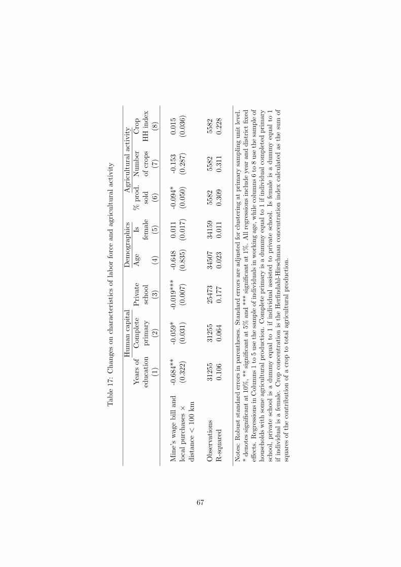
Tab

le17

:C

hang

eson

char

acte

rist

ics

ofla

bor

forc

ean

dag

ricu

ltur

alac

tivi

ty

Hum

anca

pita

lD

emog

raph

ics

Agr

icul

tura

lac

tivi

tyY

ears

ofC

ompl

ete

Pri

vate

Age

Is%

prod

.N

umbe

rC

rop

educ

atio

npr

imar

ysc

hool

fem

ale

sold

ofcr

ops

HH

inde

x(1

)(2

)(3

)(4

)(5

)(6

)(7

)(8

)

Min

e’s

wag

ebi

llan

d-0

.684

**-0

.059

*-0

.019

***

-0.6

480.

011

-0.0

94*

-0.1

530.

015

loca

lpu

rcha

ses×

(0.3

22)

(0.0

31)

(0.0

07)

(0.8

35)

(0.0

17)

(0.0

50)

(0.2

87)

(0.0

36)

dist

ance<

100

km

Obs

erva

tion

s31

255

3125

525

473

3450

734

159

5582

5582

5582

R-s

quar

ed0.

106

0.06

40.

177

0.02

30.

011

0.30

90.

311

0.22

8

Not

es:

Rob

ust

stan

dard

erro

rsin

pare

nthe

ses.

Stan

dard

erro

rsar

ead

just

edfo

rcl

uste

ring

atpr

imar

ysa

mpl

ing

unit

leve

l.*

deno

tes

sign

ifica

ntat

10%

,**

sign

ifica

ntat

5%an

d**

*si

gnifi

cant

at1%

.A

llre

gres

sion

sin

clud

eye

aran

ddi

stri

ctfix

edeff

ects

.R

egre

ssio

nsin

Col

umns

1to

5us

eth

esa

mpl

eof

indi

vidu

als

inw

orki

ngag

e,w

hile

colu

mns

6to

8us

eth

esa

mpl

eof

hous

ehol

dsw

ith

som

eag

ricu

ltur

alpr

oduc

tion

.C

ompl

ete

prim

ary

isa

dum

my

equa

lto

1if

indi

vidu

alco

mpl

eted

prim

ary

scho

ol,

priv

ate

scho

olis

adu

mm

yeq

ual

to1

ifin

divi

dual

assi

sted

topr

ivat

esc

hool

.Is

fem

ale

isa

dum

my

equa

lto

1if

indi

vidu

alis

afe

mal

e.C

rop

conc

entr

atio

nis

the

Her

finda

hl-H

irsc

hman

conc

entr

atio

nin

dex

calc

ulat

edas

the

sum

ofsq

uare

sof

the

cont

ribu

tion

ofa

crop

toto

tal

agri

cult

ural

prod

ucti

on.

67

Table 18: Alternative measures of distance

Ln(real income per capita)(1) (2) (3)

Mine’s wage bill and 0.137* 0.150** 0.134*local purchases × (0.077) (0.075) (0.074)distance < median

Measure of distance Shortest path Topographic Straightby road line

Median distance (km) 90 75 65

Observations 7738 7738 7738R-squared 0.521 0.521 0.521Notes: Robust standard errors in parentheses. Standard errors are adjusted forclustering at primary sampling unit level. * denotes significant at 10%, ** signifi-cant at 5% and *** significant at 1%. All regressions include year and district fixedeffects and control variables. Topographic distance is calculated as the length ofthe shortest path that minimizes the normalized sum of altitude and gradient.Straight line distance is the Euclidean distance between two points.

68

Table 19: Exploring the decrease of the effect by distance

Ln(real income per capita)(1) (2) (3)

Mine’s wage bill and local purchases x

distance -0.128**(0.062)

Ln(distance) -0.034**(0.016)

distance−1 0.002*(0.001)

Observations 7738 7738 7738R-squared 0.521 0.521 0.521Notes: Robust standard errors in parentheses. Standarderrors are adjusted for clustering at primary samplingunit level. * denotes significant at 10%, ** significantat 5% and *** significant at 1%. All regressions includeyear and district fixed effects. Distance is equal to thelength of the shortest path by road from the main townof the district where the household lives to Cajamarcacity, expressed in hundreds kilometers.

69

8 Conclusion

This paper investigates the effect of a large mine on a regional economy usingthe analytical framework provided by a spatial general equilibrium model.We find robust evidence that the mine has generated positive income and netwelfare gains for residents in the city and in the surrounding rural hinterland.

The main contribution of the paper is to improve the understanding ofthe mechanisms through which natural resource extraction can foster localdevelopment. In particular it shows that, in the presence of backward link-ages, the expansion of extractive industries can generate a positive demandshock and increase the real return to local factors of production, such asland and labor. In turn, this translates into better living conditions forlocal residents.

A main limitation of the paper is that we only observe events occurringover the span of a decade during the mine operation. This means that weare unable to explore whether the welfare gains are a short-term effect orpart of sustainable development that would persist after the mine closure.For the same reason, we can say little about relevant long-run phenomenasuch as specialization, technological progress, or city formation (such as SanFrancisco after the Gold Rush). Though beyond the scope of this paper,these phenomena warrants further research.

In the case we study, the positive effects come from a market channelrather than from the revenue windfall to local governments. This suggeststhat, in a context of weak governments, policies that promote local pro-curement and employment could be more beneficial to local residents thanincreased public spending, at least in the short run.

This policy implication, however, depends of the pre-existence of goodand labor markets o able to supply local inputs to the mine, and the extent ofeconomic integration of the region where the mine is located. In the absenceof inter-regional trade, the benefits would disappear since the increase ongood prices could offset the gains on nominal income. Similarly, lack of intra-regional trade or labor mobility would restrict the benefit to the place wherethe mine suppliers are located and might lead to negative re-distributionaleffects.

The availability of natural resources in the developing world is often seenas a hindrance to economic development. In most cases, institutional failure

70

(e.g. conflict, mismanagement or corruption) is at the heart of this inabilityto transform natural wealth into better standards of living. However, as thispaper suggests, in the presence of strong enough backward linkages naturalresources can be more a blessing than a curse.

71

References

Banco Central de Reserva del Peru, “Cuadros Anuales Historicos,”2009.

Benjamin, Nancy C., Shantayanan Devarajan, and Robert J.

Weiner, “The ’Dutch’ disease in a developing country : Oil reservesin Cameroon,” Journal of Development Economics, January 1989, 30(1), 71–92.

Black, Dan, Terra McKinnish, and Seth Sanders, “The EconomicImpact of the Coal Boom and Bust,” Economic Journal, April 2005,115 (503), 449–476.

Black, Sandra E., “Do Better Schools Matter? Parental Valuation ofElementary Education,” Quarterly Journal of Economics, 1999, 114(2), 577–599.

Carrington, William J, “The Alaskan Labor Market during the PipelineEra,” Journal of Political Economy, February 1996, 104 (1), 186–218.

Caselli, Francesco, “Power Struggles and the Natural Resource Curse,”2006.

and Guy Michaels, “Do Oil Windfalls Improve Living Standards?Evidence from Brazil,” June 2009.

Corden, W. Max and J. Peter Neary, “Booming Sector and De-Industrialisation in a Small Open Economy,” The Economic Journal,1982, 92 (368), 825–848.

Deaton, Angus, The Analysis of Household Surveys: A MicroeconometricApproach to Development Policy, John Hopkins University Press forThe World Bank, 1997.

Evans, William N. and Julie H. Topoleski, “The Social and EconomicImpact of Native American Casinos,” NBER Working Papers 9198,National Bureau of Economic Research September 2002.

Fujita, Masahisa and Paul Krugman, “When is the economy mono-centric?: von Thunen and Chamberlin unified,” Regional Science andUrban Economics, August 1995, 25 (4), 505–528.

72

, , and Anthony J. Venables, The Spatial Economy: Cities,Regions, and International Trade, The MIT Press, 1999.

Greenstone, Michael and Enrico Moretti, “Bidding for IndustrialPlants: Does Winning a ’Million Dollar Plant’ Increase Welfare?,”NBER Working Papers 9844, National Bureau of Economic Research,Inc July 2003.

and Justin Gallagher, “Does Hazardous Waste Matter? Evidencefrom the Housing Market and the Superfund Program,” QuarterlyJournal of Economics, 2008, 123 (3), 951–1003.

Hirschman, Albert O., The Strategy of Economic Development, Yale Uni-versity Press, 1958.

Hooker, Mark A and Michael M Knetter, “Measuring the EconomicEffects of Military Base Closures,” Economic Inquiry, October 2001,39 (4), 583–98.

Humphreys, David, “Emerging Players in Global Mining,” ExtractiveIndustries and Development Series 5, The World Bank June 2009.

INEI, “Condiciones de Vida en el Peru: Evolucion 1997-2004,” 2006.

, “Peru: Perfil de la Pobreza segun departamentos 2004-2006,” 2007.

, “Peru: Compendio Estadıstico,” 2008.

Jenkins, Beth, Anna Akhalkatsi, Brad Roberts, and Amanda Gar-

diner, “Business Linkages: Lessons, Opportunities and Challenges,”Technical Report, IFC, International Business Leaders Forum, and theFellows of Harvard College.

Koenker, Roger and Kevin F. Hallock, “Quantile Regression,” Journalof Economic Perspectives, Fall 2001, 15 (4), 143–156.

Kuramoto, Juana R., “Las aglomeraciones productivas alrededor de laminera: el caso de la minera Yanacocha S.A,” Documentos de Tra-bajo 27, Grupo de Analisis para el Desarrollo (GRADE) July 1999.

Lederman, Daniel and William F. Maloney, “Trade structure andgrowth,” Policy Research Working Paper Series 3025, The World BankApril 2003.

73

Magee, L., A. L. Robb, and J. B. Burbidge, “On the use of samplingweights when estimating regression models with survey data,” Journalof Econometrics, June 1998, 84 (2), 251–271.

Michaels, Guy, “The Long-Term Consequences of Regional Specializa-tion,” CEPR Discussion Papers 6028, CEPR Discussion Papers De-cember 2006.

Minera Yanacocha, “Balance Social,” 2002.

, “Balance Social y Ambiental,” 2006.

Ministerio de Energıa y Minas, “Anuario Minero,” 2006.

Pasco-Font, Alberto, Alejandro Diez Hurtado, Gerardo Damonte,

Ricardo Fort, and Guillermo Salas, “Chapter 4. Peru: Learningby Doing,” in Gary McMahon and Felix Remy, eds., Large Mines andthe Community: Socioeconomic and Environmental Effects in LatinAmerica, Canada and Spain, The World Bank, 2001.

Roback, Jennifer, “Wages, Rents, and the Quality of Life,” Journal ofPolitical Economy, December 1982, 90 (6), 1257–78.

Sachs, Jeffrey D. and Andrew M. Warner, “Natural Resource Abun-dance and Economic Growth,” NBER Working Papers 5398, NationalBureau of Economic Research, Inc December 1995.

and , “The big push, natural resource booms and growth,” Jour-nal of Development Economics, June 1999, 59 (1), 43–76.

and , “The curse of natural resources,” European Economic Re-view, May 2001, 45 (4-6), 827–838.

Sala-i-Martin, Xavier, Gernot Doppelhofer, and Ronald I. Miller,“Determinants of Long-Term Growth: A Bayesian Averaging of Clas-sical Estimates (BACE) Approach,” American Economic Review,September 2004, 94 (4), 813–835.

Torvik, Ragnar, “Natural resources, rent seeking and welfare,” Journal ofDevelopment Economics, April 2002, 67 (2), 455–470.

World Bank, “A Sourcebook for Poverty Reduction Strategies: Mining,”2002.

74

A Proofs

A.1 Existence of equilibrium

Assumption 5 N > 1−α1−α−µθS

This assumption means that the share of employment from the mineis small enough relative to the total population in the region. To checkhow reasonable this assumption is, note that we can re-write it as µ <

(1− α)(1− θS

N

), where α is the consumer’s budget share of locally produced

food, µ is the budget share of local manufactures and θSN is the relative size

of the mine’s workforce.We calculate the budget share on food using the ENAHO survey and

use it as a proxy for α.The estimated budget share is 0.6, however note thatthis measure may overestimate the true value of α since some of the food isnot locally produced. Regarding θS

N , recall from Section 3 that Yanacocha’sdirect and indirect employment in the analyzed period was between 12%and 20% of the active population of the city of Cajamarca. This proportionwould be significantly lower if we include working population in the restof the region. These figures imply that for Assumption 1 to be violated µ

should be, at least, greater than 0.32 or 0.35. In turn this implies a verysmall budget share of imported goods (1 − α − µ), with values at mostbetween 0.05-0.08.82

Proposition 6 Under Assumption 5, there is a unique and positive pair(f∗;w∗) that solves (AA) and (BB).

Proof. To see this, first note that we can re-write equilibrium condition(BB) as a function of Le(w) and plug it in equilibrium condition (AA). Wethen obtain an expression of f only that can be expressed as

H(f) = N − 2caf −1− α

1− α− µθS −A(f)

,where A(f) = (1 + µ1−α−µ

1ε

)ε

1− ε{2ca[ (1−α)(1−e−τf )

αe−2(1−α)τf + f ] − N}, A′(f) > 0

and H ′(f) < 0. To find the equilibrium, we look for a value f∗ such thatH(f∗) = 0.

82Note that the overestimation of α and θSN

mean that the threshold that µ shouldexceed to violate assumption 1 are understated. Hence, violation of assumption 1 requiresan even higher µ, and smaller budget share of imported goods.

75

First, recall that the values that f can adopt in equation (AA) have an

upper bound f = 12ca

(N − 1−α

1−α−µθS)

with 0 < f <N

2caunder Assumption

5. Note that H(f) = −A(f), which is negative only if 2ca[(1−α)(1−e−τf )

αe−2(1−α)τf+

f ] − N > 0. From definition of f , (11) and (16), this condition can be re-

written as 1−α1−α−µθS+

πew> 1−α

1−α−µθS

2ca, which is satisfied under Assumption

5, hence H(f) < 0.Second, recall that the values of f in equation (BB) have a lower bound

f≡ limw→∞

f = g−1 (N), where g−1 (·) is the inverse function of g(f) ≡

2ca[(1−α)(1−e−τf )

αe−2(1−α)τf +f ]. from this definition follows that A(f) = 0. Combiningthis result with the previous observations that A(f) > 0 and A′(f) > 0, it

follows that 0 < f < f <N

2caand thereforeH(f) = N−2caf− 1−α

1−α−µθS > 0.

Finally, since H(f) monotonically decreases in f , H(f) > 0 and H(f) <0 imply that there is a unique positive value f∗ ∈ (f, f), such that H(f∗) =0. From inspection of either (11) or (16), values of f∗ ∈ (f, f) imply a valueof Le(w) > 0 and thus that the equilibrium wage, namely w∗, is also uniqueand positive.

A.2 Effect on number of manufacturing firms

Proposition 7 the number of manufacturing firms, v increases with the

expansion of the mine, dvdS > 0, if and only if θ > −1

ε

dLedw

dw

dS.

Proof. Taking total derivatives to (AA) we obtain that:

−2cadf

dS− (1− α− µ) ε+ µ

(1− α− µ) εdLedw

dw

dS=

1− α1− α− µ

θ. (22)

Similarly taking total derivatives to (17) we obtain

dv

dS= −2ca

df

dS− dLedw

dw

dS− θ (23)

and thus dvdS > 0 if and only if:

−2cadf

dS− dLedw

dw

dS> θ. (24)

Using (22) and (9) we can re-write condition (24) as θ > −1ε

dLedw

dw

dS.

76

A.3 Effect on real wage

Proposition 8 if the number of manufacturing firms increase with expan-sion of the mine, then dω

dS > 0. Otherwise, the effect is more likely to bepositive for low values of µ, θ or high values of ε.

Proof. Taking total derivatives to (18) and using (13) we obtain:

dω

dS=

µ

σ − 1(w

G)µv−1 dv

dS+ 2(1− α)ατ(

w

pa)α(− df

dS)+

(1− α− µ)(w

pa)1−α−µw−1dw

dS,

(25)

which is positive ifdv

dS> 0.

To study the conditions fordω

dS> 0 when

dv

dS< 0, we first re-write (25)

replacingdv

dSusing expression (23):

dω

dS= C − dLe

dw

dw

dS− θ,

where

C ≡ −{2(1− α)ατ(w

pa)ασ − 1µ

(w

G)−µv + ca}

df

dS+

(1− α− µ)(w

pa)1−α−µw−1σ − 1

µ(w

G)−µv

dw

dS.

Hence the condition fordω

dS> 0 when

dv

dS< 0 is:

C − dLedw

dw

dS> θ.

Note, from Proposition 7, thatdv

dS< 0 implies −dLe

dw

dw

dS> εθ. That

means that a sufficient condition fordω

dS> 0 when

dv

dS< 0 is:

C > θ(1− ε).

This condition is more likely to be satisfied for high values of ε or lowvalues of µ and θ.

77

A.4 Proof of Propositions 1 and 2

Using the definition of real income from (19) and re-arranging, we can re-write the food market equilibrium condition (11) as:

paP

=[2 (1− α)

∫ f

0e−τrdr

]−1

αLy,

where y is the real income in the city. Note that dydS > 0 implies dpa/P

dS >

0, because dfdS < 0 and dL

dS > 0. However if dydS > 0 the sign of dpa/P

dS isambiguous.

Recall that real income in the rural hinterland is:

y(r) =1k

paPe−2(1−α)τ |r|.

It is immediate to see that dy(r)dS > 0 and d2y(r)

dSdr < 0.

A.5 Proof of Proposition 3

Using (2) and (5), we can write the relative prices of food and the importgood as:

pa(r)P (r)

=paPe−2(1−α)τ |r|

pm(r)P (r)

=pmPe2ατ |r|.

By proposition 1, we know that if dydS > 0, then dpa/P

dS > 0 which alsoimplies that dpa(r)/P (r)

dS > 0 Since dPdS Q 0 and dpm

dS = 0, it follows thatdpm(r)/P (r)

dS Q 0.

78