MULTIDIMENSIONAL MEASURE OF JOB QUALITY PERSISTENCE AND HETEROGENEITY IN A DEVELOPING COUNTRY

Autores: Federico Huneeus, Oscar Landerretche

y Esteban Puentes

Santiago, Mayo de 2012

SDT 357

Multidimensional Measure of Job Quality: Persistence

and Heterogeneity in a Developing Country

Federico Huneeus

Department of Economics

University of Chile

Oscar Landerretche M.

Department of Economics

University of Chile

Esteban Puentes

Department of Economics and Microdata Center

University of Chile

This Version: May 2012∗

Abstract

We adapt the multidimensional poverty methodology to study job quality dynamics using a unique

household survey panel for Chile. We use information on wages, type of contract, training and em-

ployment duration to build an aggregate job quality index. Panel data allow us to properly separate

individual heterogeneity and true dependence. We estimate a dynamic panel with random effects finding

higher job quality among larger and unionised firms. Moreover, labor history predicts job quality con-

firming the existence of persistence in job quality .

Keywords: Job Quality, Nonlinear Dynamic Panel with Random Effects, Job Persistence, Segmenta-

tion, Multidimensional Poverty Measures.

JEL Classification: C25, C43, I32, J28, J41, J81.

∗We thank Jaime Ruiz-Tagle, Kirsten Sehnbruch, Dante Contreras and Eduardo Engel for helpful comments and suggestions.

We also benefited, in an earlier version, from comments by participants at the Microdata Center Seminar (November 2011)

of the Millennium Scientific Initiative. We benefited also from comments from participants at the Seminar of the Economics

Department of the University of Chile, University Diego Portales and University of Santiago. This investigation may not have

been possible without the support of the Millennium Scientific Initiative of the Microdata Center (Project NS100041) and the

collaboration and financial support of the Sub-regional Office of the International Labour Organization (ILO) for the Southern

Cone. The usual disclaimer applies.

1

1 Introduction

In developed countries the interest in and relevance of job quality is raising exponentially (Osterman and Shulman

(2011)). However, in developing countries, this literature is almost non existent1. We are interested in study-

ing job quality because of the link between job conditions and job performance suggested in this type of

literature. Additionally, there are indications that higher quality jobs could foster productivity growth

(Davoine et al. (2008)) and would produce better life conditions and sustainable growth2. These issues are

particularly important for Chile, a country that in the past decades has combined both strong economic

growth and accelerated poverty reduction with a twin problem of low employment rates and high inequality

levels, making it a controversial development case (OECD (2009)). In Chile, productivity improvements

that fostered economic growth occurred mostly in capital-intensive sectors while job creation had been less

impressive and occurred mainly in relative low productivity service sectors, suggesting the existence of a

segmented labor market (OECD (2009))3 If the link between job conditions and job performance is true,

the evidence of a segmented growth in productivity could be traced to the determinants and dynamics of

job quality, making the study of job quality very relevant for Chile or any developing country that exhibits

similar characteristics.

Additionally, looking only at quantitative labor indicators (such as unemployment and labor participation

rates) or analysing job quality only through wages could lead to ignoring important labor characteristics, that

may be relevant determinants of labor market heterogeneities or segmentation. Some of these characteristics

may be complementary, thus analysing them piecewise may not allow us to see the big picture. The existence

of segmentation as indicated by these characteristics could indicate a stagnation in job quality improvements

in some areas of the labor market and inhibit further improvements in worker welfare and productivity4.

Then, understanding the determinants and the dynamics of job quality could contribute to provide a better

policy orientation to improve the development strategy for a developing country.

Therefore we are interested in empirically studying the determinants and dynamics of job quality for

the Chilean labor market. We are also interested in understanding if job quality comes from economic

sector and/or, firm or individual characteristics. Our working hypothesis is that due to the segmentation

documented in the Chilean labor literature (OECD (2009), Basch and Paredes-Molina (1996), and OECD

(2003)), there should be important heterogeneities in job quality across different labor dimensions (like firm

size, gender and economic sector).

The contribution of this paper is threefold. First, it proposes a new methodology to measure job quality:

an issue not solved in the job quality literature. The concept of job quality has not been standardized and

the literature on this subject is still young (see Section 2). Moreover, usual attempts go in the direction

of imposing a metric of unidimensional analysis that only partially represents conditions of job quality.

We believe that the reasons that have induced the literature to understand poverty as a multidimensional

phenomenon can also be applied to job quality: focusing on a unidimensional view could be hiding important

complementarities and ignoring some very relevant labor market failures. To construct our metric, we follow

the approach of the European Union (UE) (Davoine et al. (2008)), and of Ruiz-Tagle and Sehnbruch (2011)

for Chile. For this, we use the methodology of multidimensional poverty (Alkire and Foster (2011a)). We

1There are some exceptions, see Section 2.2The link between these two themes could be job motivation/satisfaction (Davoine et al. (2008)), informality (Perry et al.

(2007)), or a capability approach, where higher job quality is associated with more labor capabilities and thus, with higherproductivity.

3A similar argument is presented for the United States in Kalleberg (2011).4For this investigation and the literature in general, job quality is studied from the supply side (Davoine et al. (2008)).

2

gauge job quality from the supply side using four dimensions of job quality. We test and find that these

innovations aggregate value to the measurement of job quality.

Second, this paper uses a rich and complete household panel database that, mixed with a random-effects

dynamic nonlinear panel estimator, allows us to properly control the dynamics, persistence of job quality,

and individual unobserved heterogeneity (Wooldridge (2005)). The initial condition problem that arises with

dynamic panels with unobserved effects has been extensively studied (the different solutions are summarized

in Hsiao (2003)). We estimate our model following Wooldridge (2005) that solves the initial condition

problem in this setup.

The third is to contribute to a better understanding of the determinants and dynamics of multidimensional

job quality. We believe this is especially important to understand where policies should be targeted and to

increase the literature in this topic, which is especially thin in developing and emerging countries.

We use a Chilean Panel Data Household Survey called the Social Protection Survey (SPS or EPS for

“Encuesta de Proteccion Social” in Spanish) for the years 2002-2009. This is an unique survey for Chile, and

compared to other countries in Latin America. This panel has a comprehensive set of questions concerning

many relevant labor dimensions and asks the worker to retrospectively reconstruct his labor history since

1980. We extend the methodology developed by Ruiz-Tagle and Sehnbruch (2011) by applying a multidi-

mensional poverty method to correctly assess the impact of low job quality. To address this issue we apply

the vast methods of multidimensional poverty. We follow (Alkire and Foster (2011a)), which counts the

amount of deprivations individuals have across different dimensions (in our case, labor dimensions). Due to

the data features, we do not measure gaps of quality, but only the accounting of job quality. This proposed

methodology, has the benefit of being simple, applicable in diverse contexts, and decomposable in subgroups.

We identify the determinants of job quality by controlling for individual unobserved heterogeneity and

persistence in job quality. This strategy constitutes a strong robust test of the observable determinants that

survive our estimation.

We find that, first, there is no systematic heterogeneity in some of the labor attributes hypothesized like

gender, public/private and economic sector, but robust and systematic heterogeneity in job quality by firm

size and unionisation. As firm size grows by number of workers, job quality improves, also, being part of a

union is highly correlated with better job quality.5.

Second, rather than static heterogeneity, we find robust dynamic heterogeneity in job quality. There is

a strong persistence that suggests that people with low quality jobs find it hard to find better employment.

The result we find indicates that having a low quality job makes having a future low quality job more likely,

which suggest segmentation in labor markets.

Third, we check that our findings are robust to alternatives by changing the specification of the estimation

strategy, the extension of the database, the aggregation of the multidimensional index and the weights of

job characteristics.

This paper is organized as follows. Section 2 locates this paper in the job quality literature. Section 3

describes the methodology we use to gauge job quality. Section 4 presents and describes the panel data we

will use. Section 5, explains our estimation strategy. Section 6 shows the results. Section 7 discusses policy

implications and concludes.

5There’s some evidence of job quality segmentation in the US (Holzer (2011)), but this seems due to skill mismatch.

3

2 Job Quality Literature

For developing countries the issue of labor quality is particularly important, since jobs do not necessarily

meet minimum quality standards (Streeten (1981) and Frieden et al. (2000) for example). The question is:

do lower unemployment rates guarantee better working conditions? Although in general it is better to be

employed, it’s not sufficient to limit analysis to employment rates if one is interested in studying reality

of labor markets in developing countries. This is because the type of work is relevant to analyze welfare

characteristics of jobs. If there are no labor standards, studying only quantity indicators is not sufficient to

address the problems in the labor markets.

The literature of job quality economics is young but very heterogeneous. Since the 1970s indirect but

related subjects have been developed in the literature in areas akin to economics, like sociology and psycho-

logy. The traditional view associates job quality with wages (Abowd et al. (1999)). However, many have

argued that this is a narrow interpretation. They refer to related concepts like job satisfaction (Freeman

(1978) and Judge et al. (2001)), stability (Stewart (2007)), social security (Kalleberg et al. (2000)), security

(Dewan and Peek (2007)), informality (Perry et al. (2007) and Gunther and Launov (2012)), and contracts

characteristics (Clarke and Borisov (1999) and Ruiz-Tagle and Sehnbruch (2011)). In Europe, other job

quality concepts have been developed like family and employment (Menaghan et al. (2000) and Presser

(2000)), psychological health related to job quality (Burchell (1994) and Nolan et al. (1999)) and organiza-

tional work, and job quality (Gallie (2007) and Green (2001)).

At the end of the 1990s, the International Labour Organization (ILO) launched the concept “De-

cent Work” (ILO (1999)). This concept strongly impacts the literature related to ILO (for Chile, see

Infante and Sunkel (2004)). However, Decent Work has a bounded influence in the non-ILO literature.

Despite this, the general influence of promoting the debate has been strong and they have developed new

concepts like non-discrimination and social dialogue, e.g. more social participation. Subsequently in Europe,

new related concepts start to emerge: good jobs (Duffy et al. (1997)), precariousness (Kalleberg (2009) and

Barbier (2002)) and underemployment (Bescond et al. (2003)). The Oxford Poverty and Human Develop-

ment Initiative (OHPI) has also developed related issues, which have been applied to Chile (Cassar (2010))

to general ways of measuring job quality (Lugo (2007)).

At the same time, the European Union in the last 20 years has systematically standardized labor norms

and since 20006 has tried to create quality indicators (like the Job Quality Indicators supported at the

Laeken European Council in December 2001 and followed by Davoine et al. (2008)). Some other experiences

in Europe have applied statistical tools to generate job quality indicators, but those efforts have been

sporadic and vague. It is common to find indicators that describe and synthesize the features described

above, but almost none actually build multidimensional indicators. They are mainly focused on promoting

unidimensional indicators of other variables beyond employment, unemployment, participation rates, and

wages.

So, the job quality literature has been developing different concepts to focus the debate and see how to

best study job quality. Some are starting to focus on the multidimensional scope of measuring job quality.

But there is still much to do on this.

This subject is particularly undeveloped in the case of developing countries. For example, for Chile we

have a working paper of Ruiz-Tagle and Sehnbruch (2011) (onwards, RTS) that analyzes different ways of

measuring job quality. We will follow the work done in this direction.

6Since the job quality issue was first introduced at the Lisbon Council in March 2000.

4

3 Measuring Job Quality for Chile

One of the big problems recognized in the very recent job quality literature is the issue of measurement of a

multidimensional phenomenon. Despite the differentiated efforts (commented in Section 2) we recognize that

there is still no standard or agreed definition in the academic literature to summarize job quality in a synthetic

indicator. We suggest that reducing the study of job quality to a piecewise unidimensional analysis could

hide important complementarities and thus make it difficult to compare workers. In developed countries,

there is a growing consensus that job quality, like poverty, must be understood through a multidimensional

analysis (Davoine et al. (2008)). We propose a way of doing this for developing countries.

In ideal terms, once the concept of job quality is defined, one has to deal with at least four challenges

to build a multidimensional indicator for job quality. The first is data availability. This will determine

if the analysis will be at the worker or firm level, and if it will be at an objective or subjective level.

The ideal way to measure job quality in a multidimensional way is to include both worker characteristics

and firm characteristics7 both subjectively, e.g. from the perceptions of workers or firms, and objectively

from observational data. There are few studies that consider analysis on both demand and supply sides

(Holzer et al. (2011) and Judge et al. (2001)). It is very likely that this is a result of data limitations since

we have not found a survey that includes all four of the aspects mentioned.

The second problem is defining which labor dimensions are relevant to job quality (either in the demand

or supply side). Are the most relevant dimensions cardinal (like income) or ordinal variables (like scores for

contract quality). The best contribution to this effort has been done by the International Labour Organ-

ization (ILO) with the introduction and advertisement of the “Decent Work” concept (ILO (1999)) which

required a systematization of the dimensions (mainly on the supply side) that needed to be considered in

order to talk about “Decent Work” (Anker et al. (2003), and Bescond et al. (2003), for example).

The third issue is defining the method of identifying a low quality job and aggregating the different

dimensions chosen. Identification of what is a low quality job is one of the most difficult challenges; the

literature is very under-developed for this question. On the other side, in terms of aggregation, most of

the ILO related research has developed indicators for each dimension proposed separately, but no one has

proposed a synthesized way of treating all of them8. A method of aggregation could be weighted averages over

different labor dimensions (standardizing or scoring in order to make the dimensions comparable9) or more

sophisticated aggregation like the ones developed by the literature on multidimensional poverty measures

(for a discussion on the literature on this, see Alkire and Foster (2011b) and Alkire and Foster (2011a)).

Finally, the fourth challenge is defining how to weight the different labor dimensions when aggregating

them. One option is to weight them according to an empirical definition; the other is to weight them in

reference of a theoretical definition. Once these four issues are addressed, building a multidimensional job

quality index is possible.

3.1 Measuring Job Quality for Chile: The RTS Measure.

Ruiz-Tagle and Sehnbruch (2011) implement an aggregate job quality index applied to the Chilean case. We

will base part of our methodology on their work, but we will aggregate the job quality dimensions differently

using a multidimensional index.

7Most of the economic literature on job quality treats it as a supply side issue. Thus job quality is understood as a conceptthat determines workers welfare rather than firm output (see Davoine et al. (2008) and Johri (2005) for example).

8The only exception seems to be Peek (2006), to which we have no access for being an internal document of ILO.9Similar to what Ruiz-Tagle and Sehnbruch (2011) do for Chile.

5

They address the four challenges10 as follows. First, they use two household surveys with information on

workers, not firms. Second, they use four labor dimensions: (1) income, (2) contracts and social protection,

(3) tenure and (4) training. The data they used is at an individual level and allows measurement of each

dimension for every worker. These four dimensions are measured in an objective way. As every dimension

has a different metric;11, they assign scores ranging in the [0, 2] interval for every dimension, to make them

comparable and additive. The scores are showed in Table 1.

Table 1: Scores assigned to the four Labor Dimensions (Ruiz-Tagle and Sehnbruch (2011))

Level of Income Score

More than 4 Minimum Wages 2

From 2 to 4 Minimum Wages 1

Less than 2 Minimum Wages 0

Contracts and Social Protection Score

Permanent Contract with Contributions 2

Permanent Contract without Contributions 1

Atypical Contract with Contributions 1

Atypical Contract without Contributions 0

No Formal Contract 0

Job Tenure Score

More than 5 years tenure 2

From 1 to 5 years tenure 1

Less than 1 year tenure 0

Training Score

Trained in the actual job 1

Not trained in the actual job 0

They use these four dimensions due to data availability and relevance for job quality analysis. Since we

are going to use only if each of these variables are zero or different from zero, we refer only to the zero score

justification of each dimension.

Income is measured by the last monthly wage received by the worker12. The idea is to measure if the

worker is achieving a purchasing power that allows the household to be over the poverty line. So a worker

will have more than 0 at her income score, if she earns more than 2 minimum wages (required in order that

a low income household be able of being over the poverty line). It would be of interest to consider also

the stability (not only the level) of income, but they assume this will be captured by the other dimensions

(specially tenure).

Contracts and Social Protection is measured by the temporality of contracts and if the worker contributes

to his pension savings (and thus has some level of social protection), respectively13. As the worker contract

gets permanent (that means it is a long-term contract) and meets with the requirement of contributing to

pension savings14, the worker gets higher scores in this variable. Not having a formal contract is the worst

scenario for the worker: it implies no legal entitlements, and no health insurance or pension savings.

Job Tenure is measured as the time the worker has been in the actual job. It is relevant because longer

tenures are associated with severance payment rights (after one year of working with a permanent contract),

which is why increases after one year of tenure in the RTS methodology, unemployment insurance benefits

and job stability that generates better planning and long-run investments conditions. If a worker has more

than 5 years tenure it has access to severance payments and also to unemployment insurance benefits that

allow him to finance an average of 5 months of unemployment during non-crisis periods.

10Described at the beginning of Section 3.11For example, the income dimension is measured through wages, that are continuous and cardinal while the training dimen-

sion is discrete and ordinal, it is equal to one if the worker has been in trained and zero otherwise.12To see the relevance of wages for job quality and job satisfaction, check Section 2.13To see the relevance of this feature in job quality literature, see Section 2.14Having a permanent contract doesn’t ensure compliance with contribution regulations.

6

Finally, training is measured as if the worker has been trained in his job15. This dimension is relevant

because being trained in a job usually involves a combination of general human capital skill acquisition and

specific human capital that may induce productivity improvements16.

Considering these four characteristics, each worker will have a score according to her personal job char-

acteristics. The third challenge is to define an aggregation method. The RTS Measure aggregates in the

following way:

Job Quality = Income+ Contract Social Protection+ Tenure+ Training

Where the job quality aggregated index is the sum, for each worker, of the scores of the four dimensions.

Thus, the index lives in the [0, 7] range, with 7 as the highest quality level. The fourth challenge, weighting

the different labor dimensions, are solved without estimating empirical nor theoretically. They weight every

dimension the same.

We will use the same four dimensions to study job quality mainly because these are characteristics we

can follow periodically in national surveys, we can preserve comparability between the main two household

surveys in Chile, and these are dimensions used by ILO and the UE, although these organization propose

more dimensions to study job quality.

The Multidimensional Measure of Job Quality (MIJOB) we introduce in the next sub-section 3.2 over-

comes a main drawback of the RTS measure. It proposes a way of assessing the job quality more exactly.

In the index of Ruiz-Tagle and Sehnbruch (2011), they can only say if a worker has more or less job quality

than another or if the job quality has increased or diminished with respect to a certain moment in time.

But at a particular moment, the RTS measure cannot assess if a particular level of job quality is high or

low, or how many people have low quality jobs. We will contribute to the analysis of job quality with more

economic intuition.

We will attend these challenges directly in what follows, and present more key features of the measure

we propose.

3.2 Measuring Job Quality for Chile: Our proposal

3.2.1 A New Multidimensional Index of Job Quality (MIJOB).

We will base our work on the multidimensional poverty literature. Following the conceptual work of Am-

artya Sen on capabilities (Sen (1983) and Sen (1999) for example) the literature has agreed that poverty is

better understood as a multidimensional phenomenon (Streeten [1981], Atkinson (2003), Duclos and Araar

(2006), among others). There is a vast and growing literature on how to measure multidimensional poverty

(Bourguignon and Chakravarty (2003) and Alkire and Foster (2011a)). Following this literature, we value

the quality of a job using a multidimensional poverty approach.

We will use the traditional multidimensional measure proposed by Foster, Greer and Thorbecke (in

Foster et al. (1984), FGT onwards) and conceptually revisited by Alkire and Foster (2011a) and the original

authors in Foster et al. (2010). This is the simplest and most general measure of multidimensional poverty

that we can apply to job quality and it is the best approach because it values job quality as a phenomena

of different states. This is helpful to embody more economic intuition to the results. The literature of

multidimensional poverty has advanced towards the deepening of poverty intensity measures through adjus-

15See Jones et al. (2009) for the relationship between training and job satisfaction.16Besides the fact that there is an investment in the relationship and the projection inside the firm.

7

ted versions of the FGT methodology that considers and analyses poverty gaps. These measures take into

account not only a person’s poverty, but also how deeply she is impoverished. Namely, they have recently

proposed (Alkire and Foster (2011a)) a measure for poverty gaps that go beyond poverty deprivation ac-

counting. Though these measures are more sophisticated and include more information, we stick closely to

the original FGT methodology because: (i) as we are attempting a new approach for job quality, it’s import-

ant to keep things simple, and (ii) we are using both ordinal variables and cardinal ones which complicates

the measurement of gaps. Studying gaps in ordinal variables with cardinal variables seems to lack economic

intuition. We will focus the measure of multidimensional quality from a deprivation accountability scope

than through a gap deprivation depth.

Foster et al. (2010) emphasize the goodness of this FGT measure. It has a simple structure, and its

axiomatic properties are sound17 and include the useful properties of additive decomposability and subgroup

consistency. This allows us to decompose the index of subgroups in a consistent way. The publication

of the FGT measure in 1984 produced a huge subsequent literature and applications, constituting one of

the most popular ways of defining multidimensional poverty (Foster et al. (2010)). One of the assumptions

required in order to construct this measure is that the dimensions considered need to have some degree of

complementarity. Otherwise summarizing the dimensions in one variable would not be pertinent. If the

dimensions were substitutes, the methodology would not be effective in data usage.

We emphasize that the methodology that we propose is appropriate for this context because of two

main reasons: (i) the poverty phenomenon is similar to the employment phenomenon and they are in fact

economically connected, although they use different dimensions; and (ii) because this methodology, as said,

has been used and proved in the economic literature and it is simple and intuitive.

Following the FGT measure (and the notation of Alkire and Foster (2011a)), the MIJOB measure we

propose for job quality is:

M0t =

∑ni=1 cit(k)

nd

Where cit =∑d

j=1 gjit is the amount of deprivation of worker i, d is the total labor dimensions considered

(in this case d = 4), n is the number of workers in the sample, and gjit is equal to 1 if the worker i is deprived

in that attribute j at time t. Additionally, cit is a variable defined as:

cit =

cit if cit ≥ k

0 ∼(1)

Where k is the number of deprivations defining a job of low quality. So, if cit ≥ k the worker i has a job

of low quality in moment t. Then cit is a censored variable, due to the fact that the workers with high job

quality have zero deprivations.

The interpretation of this indicator M0t is: the amount of deprivations in a specific moment t, that

workers of a specific group of size n have in relation to the total possible amount of deprivations that they

could have (nd). So M0t ∈ [0, 1]. A worker has worse job quality, according to this, when he is deprived in

more labor dimensions. Thus, higher deprivation levels imply lower job quality.

17Like monotonicity, transfer and sensitivity. These three axioms are associated with the first three orders of stochasticdominance

8

To define this index, the FGT measure uses two thresholds18:

1. One that defines deprivation in every labor dimension. For example, an individual is deprived of income

if he earns less than twice the minimum wages.

2. A threshold k, that corresponds to the amount of deprivations that define a low quality job. For

example, if k = 3, a worker will have a job of low quality if he has more than 3 deprivations.

For the first type of threshold, we will use a variation of Ruiz-Tagle and Sehnbruch (2011). We use these

scores in order to define if an individual is deprived or not in each labor dimension used and also to maintain

certain comparability with the RTS measure. See the scores in Table 1 for more details.

We only change the income dimension scores with respect to RTS. We do not use the minimum wage

but instead the Household Ethical Income (HEI) that represents a central policy of the Government of Chile

through the conditional transfer program “Chile Solidario”, which has been the main anti-poverty policy in

the last decade.

We already explained the reasons behind the scores in the sub-section 3.1. We stress that the variables

used are part of the ILO and UE and are considered to measure job quality. But there are more relevant

labor dimensions that we do not consider, which the ILO does, mainly due to data restrictions. Social

dialogue and discrimination are a few examples of these type limitations. However, the variables we choose

reflect the majority of the available data regarding job quality.

In order to apply the multidimensional poverty methodology, we need to define the threshold for defining

if a worker is deprived in each dimension. A worker is deprived in each dimension if:

1. Income: his wage is less than the Household Ethical Income for the current year (2009 = CP$250.000).

2. Tenure: he has been working at his current job for less than a year.

3. Training: the job has not provided training.

4. Contract: he does not have a formal contract, has an atypical contract without contributions, or has

been working more than one year but for short term formal fees.

These thresholds are analogous to defining deprivation in a dimension if the score of that dimension is 0.

We will not establish a priori the second type of threshold as the poverty literature usually does. We

prefer to report estimations with the four possible thresholds available for our paper. So, if we are estimating

with k = 2, a worker will have a work of low quality if he has 2 or more deprivations.

As we said, this novel methodology applied to job quality contributes to find a more synthetic way of

defining low job quality. We shall see in the data and results section how much robustness this methodology

adds.

We recognize that another option would be to generate a continuous variable of job quality using a

weighted sum of each dimension. This continuous variable could reflect job satisfaction, but the main

drawback in doing this is that it does not help to solve one of the open questions that the RTS measure

leaves open, how to define a low quality job. The multidimensional index solve that issue since, low quality

is defined if the number of deprivations of the worker is higher than the threshold k. The advantage of using

a continuous variable, however, is that it would allow us to use a linear dynamic panel instead of a nonlinear

one, but again, we would lose the main measure - how to define a low quality job. That’s why we use the

discrete multidimensional poverty index proposed here.

18Two cutoffs, as the literature treats them (Alkire and Foster (2011a)).

9

4 Data and Gross Heterogeneity of Job Quality

One of the contributions of this investigation is that we use a rich household panel data that considers broad

information of different labor situations as well as personal characteristics, and at the same time includes

the labor history of the worker since 1980. This will allow us to better understand the dynamics of job

quality. The panel data we use is the Social Protection Survey (EPS) for the years 2002, 2004, 2006, and

2009. This is the richest panel survey in Chile and constitutes a unique database for an emerging country. To

contrast the descriptive statistics we compare the characteristics of the EPS with the National Socioeconomic

Characterization Survey (CASEN) for the years 2000, 2003, 2006, and 2009. This latter survey is used to

measure the official poverty rates in Chile and has been a crucial input for the formulation of public policy

by the Chilean government for many years.

The EPS reports longitudinal data of the labor market and the social protection system. It started in

2002 as a survey for individuals that at leeast one month contribute to social security and has been repeated

in 2004, 2006 and 2009. It has had national representativeness since 2004. One major feature of this survey

is that has the labor history of the interviewee since 1980 and other characteristics like education, health and

labor training. It is also carried out more regularly than CASEN. The CASEN has an employment section,

however it is not longitudinal so we cannot use it to control for individual heterogeneity and to identify

persistence in job quality. The only inconvenience of using the EPS is that the sample size is smaller than

CASEN.

We will use both surveys to construct descriptive statistics of job quality gross heterogeneity across

different employment characteristics (like firm size). With the EPS, we build a balanced panel for the period

2002-2009. This will allow us to study the dynamics and heterogeneity because we will be able to control

for individual unobservable heterogeneity. It’s important to highlight that in order to add more years to

our sample, we include data from 2002, which implies restricting the sample to workers affiliated with the

pension system19. We also bound the analysis to employees who have been working as employees for the

entire period20.

We emphasize that we perform our analysis only for employees because job quality decisions are different

for employees that for employers or independent workers. Employees have less control over their job quality.

So mixing them together in the same analysis would not be accurate or economically intuitive. Despite

this, we will perform a robustness check to see whether our main results change when our sample includes

employers and independent workers.

The variables we are going to use as covariates in our regressions can be summarized in three groups. The

first group considers information from the worker. We use dummies for education level (primary, secondary

or tertiary), and mother’s education at the same levels; a dummy variable for gender (=1 for men); age of

the worker and squared age; and a dummy variable if the worker belongs to a union. The second group of

variables is from the firm side. We use dummy variables for each firm side, using the number of workers

(micro firms are omitted), a dummy variable equal to one if the firm is public, and one dummy for each

of nine economic sector. The third type of variables relate to the self-reported history of the worker. We

measure actual working experience and its squared, proportion of the labor history that the worker has been

working in a micro, small, or medium sized firm, and the proportion of time that the worker has been inactive

or unemployed before 2002. Besides this, we also include the lag of job quality. In Table 2, we include a

detailed description of the variables used.

19Defined as those of have made contributions to their pension savings at least once since 1980.20See sub-section 6.3 for robustness checks including employers and independent workers

10

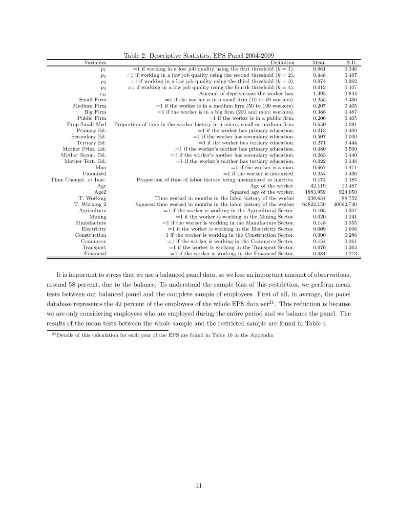
Table 2: Descriptive Statistics, EPS Panel 2004-2009Variables Definition Mean S.D.

p1 =1 if working in a low job quality using the first threshold (k = 1). 0.861 0.346p2 =1 if working in a low job quality using the second threshold (k = 2). 0.448 0.497p3 =1 if working in a low job quality using the third threshold (k = 3). 0.074 0.262p4 =1 if working in a low job quality using the fourth threshold (k = 4). 0.012 0.107cit Amount of deprivations the worker has. 1.395 0.844

Small Firm =1 if the worker is in a small firm (10 to 49 workers). 0.255 0.436Medium Firm =1 if the worker is in a medium firm (50 to 199 workers). 0.207 0.405

Big Firm =1 if the worker is in a big firm (200 and more workers). 0.388 0.487Public Firm =1 if the worker is in a public firm. 0.206 0.405

Prop Small-Med Proportion of time in the worker history in a micro, small or medium firm. 0.650 0.391Primary Ed. =1 if the worker has primary education. 0.213 0.409

Secondary Ed. =1 if the worker has secondary education. 0.507 0.500Tertiary Ed. =1 if the worker has tertiary education. 0.271 0.444

Mother Prim. Ed. =1 if the worker’s mother has primary education. 0.480 0.500Mother Secon. Ed. =1 if the worker’s mother has secondary education. 0.263 0.440Mother Tert. Ed. =1 if the worker’s mother has tertiary education. 0.022 0.148

Man =1 if the worker is a man. 0.667 0.471Unionized =1 if the worker is unionized. 0.254 0.436

Time Unempl. or Inac. Proportion of time of labor history being unemployed or inactive. 0.174 0.185Age Age of the worker. 42.119 10.487

Age2 Squared age of the worker. 1883.959 924.050T. Working Time worked in months in the labor history of the worker 238.634 88.752

T. Working 2 Squared time worked in months in the labor history of the worker 64822.150 40062.740Agriculture =1 if the worker is working in the Agricultural Sector. 0.105 0.307

Mining =1 if the worker is working in the Mining Sector. 0.020 0.141Manufacture =1 if the worker is working in the Manufacture Sector. 0.148 0.355

Electricity =1 if the worker is working in the Electricity Sector. 0.009 0.096Construction =1 if the worker is working in the Construction Sector. 0.090 0.286

Commerce =1 if the worker is working in the Commerce Sector. 0.154 0.361Transport =1 if the worker is working in the Transport Sector. 0.076 0.264Financial =1 if the worker is working in the Financial Sector. 0.081 0.273

It is important to stress that we use a balanced panel data, so we lose an important amount of observations,

around 58 percent, due to the balance. To understand the sample bias of this restriction, we perform mean

tests between our balanced panel and the complete sample of employees. First of all, in average, the panel

database represents the 42 percent of the employees of the whole EPS data set21. This reduction is because

we are only considering employees who are employed during the entire period and we balance the panel. The

results of the mean tests between the whole sample and the restricted sample are found in Table 4.

21Details of this calculation for each year of the EPS are found in Table 10 in the Appendix

11

2009Employees Panel Significance

Variables Mean Mean Mean Testp1 0.94 0.91 ***p2 0.56 0.45 ***p3 0.16 0.08 ***p4 0.03 0.01 ***

Wages per Hour 0.70 0.80 ***Training 0.11 0.14 ***Tenure 34.52 37.17 ***

Contracts 1.63 1.81 ***Small Firm 0.25 0.26

Medium Firm 0.21 0.22Big Firm 0.34 0.37 **

Public Firm 0.17 0.21 ***Primary Ed. 0.23 0.21 *

Secondary Ed. 0.50 0.51Tertiary Ed. 0.26 0.28

Mother Primary Ed. 0.46 0.48Mother Secondary Ed. 0.27 0.26Mother Tertiary Ed. 0.04 0.02 ***

Men 0.62 0.67 ***Unionized 0.21 0.28 ***

Age 42.52 44.79 ***Agriculture 0.11 0.10

Mining 0.02 0.02Manufacture 0.12 0.14 **

Electricity 0.01 0.01Construction 0.11 0.09 ***

Commerce 0.17 0.15 *Transport 0.08 0.08Financial 0.08 0.08

N 6040 2560Significance at: *** p < 0.01, ** p < 0.05, * p < 0.1

In Table 422, we can see that our balanced panel data has a higher proportion of unionized workers,

more men, more public firms, bigger firms, and different sector composition. Though these differences are

nor systematic, our panel has less proportion of workers in agriculture, construction and commerce and

more in manufacture. At the same time, our panel has more educated workers, although with less educated

mothers. Those differences are statistically significant. Although there are some biases in restricted panel

data, implying that we use a more privileged sample of workers, differences are not dramatic. Additionally,

we are considering a sample of workers with higher human capital, so finding persistence in job quality for

this sample should, in principle, be more difficult than in a sample of the whole population of employees.

Having higher human capital should imply constant improvements of job quality during time. Thus, our

results could be interpreted as a lower bound on persistence. Despite this, we will perform robustness analysis

in order to check if our main results change when amplifying the database to employers and independent

workers.

We present a gross descriptive heterogeneity of job quality to begin to understand the correlations of job

quality, and we will compare it with CASEN results to see the representativeness of our panel data.

In what follows, due to the fact that the MIJOB indicator measures the proportion of deprivations

(defined in Section 3.2) in the population, a greater level of the index implies lower job quality.

22In this table, pi with i ∈ [1, 2, 3, 4], is the probability of having a low quality job according to the four thresholds defined inSection 3.2. Wages and tenure are presented as amount of deprivations in the sample, according to the definitions of deprivationin that dimensions presented in Section 3.2.

12

Figure 1: MIJOB for each deprivation threshold k ∈ [1, 2, 3, 4]. Employees Casen 2009 and Employees EPS2009

We calculate our job quality measure using CASEN and the EPS (Figure 1). For each figure we use

the entire sample of employees. We can observe there is a slow upward trend in EPS that is followed in

CASEN, except for CASEN 2009, which shows a significant improvement in quality. The change in 2009

can be explained by a higher unemployment rate that changes the composition of workers. One could argue

that during an economic crisis, unemployment raises for workers with lower quality Jobs. There are also

some methodological changes in the fieldwork of the 2009 CASEN survey. This calls for carefulness when

interpreting these results. In any case, we do not observe a systematic improvement in job quality through

the decade.

In Figures 2 to 5 we check for gross heterogeneity in the usual observable characteristics of interest.

Figure 2: MIJOB between Firm Size, for each deprivation threshold k ∈ [1, 2, 3, 4]

13

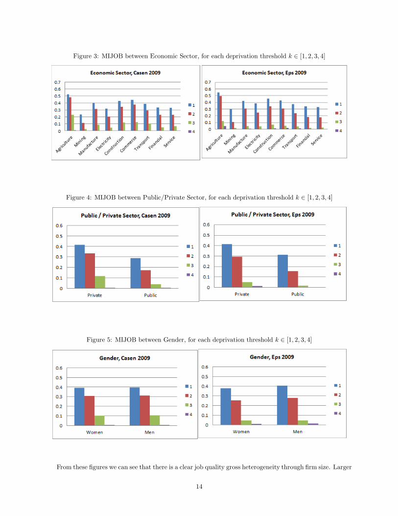
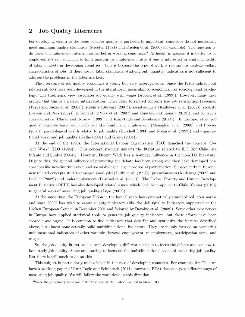
Figure 3: MIJOB between Economic Sector, for each deprivation threshold k ∈ [1, 2, 3, 4]

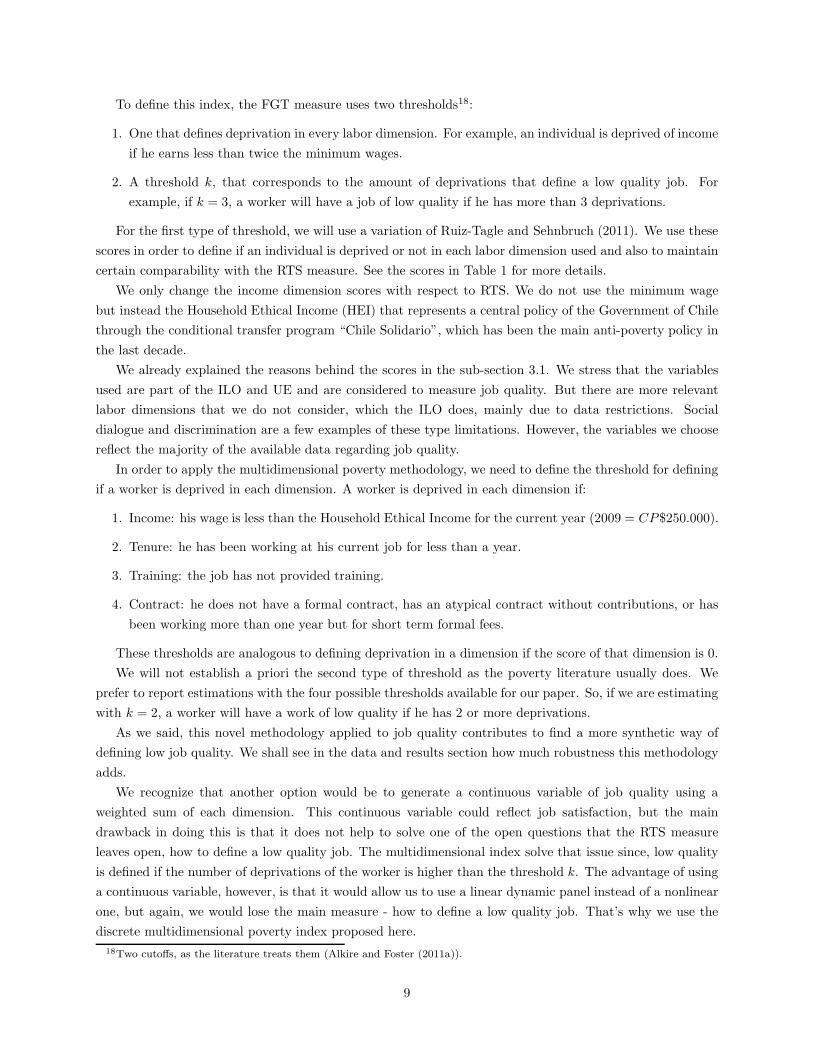
Figure 4: MIJOB between Public/Private Sector, for each deprivation threshold k ∈ [1, 2, 3, 4]

Figure 5: MIJOB between Gender, for each deprivation threshold k ∈ [1, 2, 3, 4]

From these figures we can see that there is a clear job quality gross heterogeneity through firm size. Larger

14

firms have higher job quality. The economic sectors with higher job quality are mining, services (including

financial services) and electricity. The worse are agriculture, construction, manufacture and commerce.

There is an evident gross heterogeneity through sectors. On the other hand, the public sector seems to have

better job quality than the private sector. This fact is persistent since 2000. Finally, men have lower quality

jobs, although the differences are not significant. This is a controversial result because it is well documented

in Chile (Hausmann et al. (2008)) that women have average wages around 30 percent lower than men’s.

Important selection bias and composition effects could explain the null difference in quality documented in

this paper. For example, it is possible that due to the major presence of men in the labor market, there is a

downward bias for job quality. This is an interesting stylized fact for further research.

5 Estimation Strategy

The main objective of our estimation strategy is to study heterogeneity and persistence. By heterogeneity,

we mean the differences in job quality after accounting for the lag of job quality, and individual unobserved

heterogeneity. If a variable from the individual or the firm, continues to be significant after these controls,

we will consider that there is heterogeneity in job quality in that variable. Heterogeneity means robust

differences in job quality according to a certain labor characteristic. There is persistence in job quality if the

lag of job quality is significant after controlling for observed and unobserved heterogeneity. Additionally we

will study the long term implications of persistence in labor markets. The way we will look at heterogeneity

will be completely static. Persistence, on the other hand, will be a profoundly dynamic characteristic.

In a dynamic model, it is important to account for individual heterogeneity and persistence at the same

time. If we did not do this, we could confuse persistence with a spurious correlation23. A dynamic model

with individual heterogeneity allows us to identify true dependence as defined by Heckman (1981) and

Heckman and Borjas (1980). This type of models requires panel data and, therefore, is rarely estimated for

developing countries. However, one of the limitations of our research is the potential endogeneity in variables

such as firm size or economic sector. Individuals can choose employment base on these firm characteristics.

We are not controlling this matching process. Therefore, our results are going to show us strong correlations

(due to the dynamic controls we are including), but not causality. Further research will be necessary to

investigate this issue.

In this framework we deal with two connected, but different challenges. First, defining the heterogeneous

individual effect as random or fixed, and second in dealing with the initial condition problem. For the first

challenge, if our sample had a sufficiently large T, this would not be a relevant issue, since both methods

would lead asymptotically to the same results. But since our T is finite, fixed and small, it becomes a relevant

problem, especially when wanting to estimate through fixed effects. This method, in the presence of a small

T, takes us to the problem of incidental parameters, and there is no simple transformation to eliminate this

problem in a nonlinear models like ours. Estimating a fixed effects model with small and fixed T transmits

the inconsistency of the incidental parameters24 into the other coefficients. Due to these problems, we prefer

to estimate considering the unobserved effects random25.

23There is persistence when the experience of a current event could affect the future, in relation to an identical individual thatdid not experience it. This would be true dependence. But if there are unobservable characteristics (e.g. ability or preferences)that can affect the probability of the event, but are not influenced by the experience of the event, and are correlated in time,we could estimate stability in an event only because it is a proxy of these unobservable features. This case would be spuriousstate dependence.

24Except in very special cases. See (Neyman and Scott (1948) and Hsiao (2003), for example).25This way we do not consider the recent approach proposed by Carro (2007) who uses fixed effects models.

15

The second challenge is the initial condition problem that arises in dynamic panel data models with

unobserved random effects 26. In linear models when the unobserved effects are additive, it is possible to

apply a suitable transformation, like differencing, to eliminate the individual unobservable effects. For non-

linear models, there are no general and known transformations27. For our dynamic nonlinear panel data we

use the simple solution proposed by Wooldridge (2005). He reconsiders the initial condition problem in a

parametric framework28. His approach is to model the distribution of the unobserved effects conditional on

the initial value of the dependent variable and any exogenous explanatory variables that are constant over

time. This is held over four assumptions. First, the dynamics must be of first order once the exogenous

variables and the unobserved heterogeneity are conditioned. Second, the unobserved effect is additive inside

the standard normal cumulative distribution function. Third, the covariates are strictly exogenous. Four, as

we are in a parametric framework, the econometrician must specify an auxiliary conditional distribution for

the unobserved heterogeneity. Wrongly implementing this assumption can lead to inconsistent parameters.

Wooldridge (2005) proposed, in general terms, a distribution D(·) of any dependent variable yit, such

that:

D(yit|xit,yit−1,hi) = D(yit|xi,yit−1, ...,yi0,hi)

In which xit corresponds to exogenous variables and hi to the unobserved heterogeneity. The D(|)

function can be estimated consistently and with coefficients asymptotically normal, controlling for xit, yit−1,

yi0 (the initial condition of the dependent variable) and xi (exogenous covariates that are stable in time).

The important assumption is to define a distribution, g(·) for hi conditional on (yi0,xi). This way, the

author proposes to integrate out the unobserved heterogeneity and consistently incorporate the persistence

of the dependant variable with the following log-likelihood function for each observation i:

ℓi(θ, δ) = log

[

∫

RJ

(

T∏

t=1

ft(yit|xit,yi,t−1,h; θ)

)

g(h|yi0,xi; δ)η(dh)

]

Where η(dh) is the σ-finite measure over which the model assumed, g(h|y0,x; δ), for the density of the

unobserved heterogeneity, D(hi|yi0,xi), is correct.

Following this setup, we estimate a dynamic random effect model using the EPS 2002-2009 panel that

considers unobserved heterogeneity and labor history to have a robust measure of observed heterogeneity.

We will use two models inside this framework.

The first is a dynamic probit model where the dependent variable is 1 if the worker has a low quality job.

Given that we are interested in controlling for the unobserved heterogeneity and the dynamics (persistence),

we estimate, following Wooldridge (2005):

y∗it = δ1pkit−1 + δ0pki0 +Xitα+ Zitβ +Hitγ + εit (2)

pkit = 1[y∗it ≥ 0] (3)

26Unless we assume that the initial observations are random and therefore there is independence between these observationsand the unobserved effects. Assuming this would be very strong.

27There are some special cases like the one proposed by Chamberlain (1992), Honore (1993), and Honore and Kyriazidou(2000).

28A “semiparametric identification hinges on some strong assumptions concerning the strictly exogenous covariates”(Wooldridge (2005)).

16

Where i indexes the agent (worker), t the time; 1[·] an indicator function, equal to 1 if the argument is

true, y∗ is a latent variable associated with labor dissatisfaction29. In this case, pkit = 1 if the agent i has a

low quality job at the moment t according to the threshold k ∈ [1, 2, 3, 4]. As said in a previous example, if

p2it = 1, it means that the agent has a job of low quality when she has cit ≥ 2 (corresponding to k = 2). At

the same time, Xit are worker covariates , Zit firm covariates and Hit worker labor history covariates. Also,

pkit−1 and pki0, are equal to 1 if the agent had a low job quality the last period of the panel and the initial

period of the panel, respectively.

This model will be estimated with a dynamic probit with random effects, correcting for the initial

condition and controlling for unobserved heterogeneity following Wooldridge (2005).

The second model is an ordered probit model where the dependent variable is the amount of labor

deprivations cit as described before, with the only difference that it is not censored according to the threshold

k. So cit will be the amount of deprivation a worker has 30. Like the model just described, we consider the

unobserved heterogeneity and dynamics in the estimation. The other difference is that now, as cit takes on

values in {0, 1, 2, 3, 4}, the ordered probit includes 4 lagged indicators, 1[cit−1 = j] with j = 1, 2, 3, 4. The

underlying latent variable model would be c∗it = δ1rit−1 + δ0ri0 +Xitα+ Zitβ +Hitγ + εit. Where the new

thing is rit−1, which is the vector of the lagged indicators and ri0 the vector of the same indicators as the

initial condition, as Wooldridge (2005) suggests. To estimate this model, we use a dynamic ordered probit

model with random effects31.

6 Results

6.1 Dynamic Probit with Random Effects

First, we estimated without controlling for unobserved heterogeneity and persistence. The results of the

estimation are not reported, but, overall we find that without considering unobserved heterogeneity and

persistence, the estimations of the parameters of the models are significantly higher and more significant. In

other words, controlling by these two features constitutes a robust and demanding test for our covariates32.

When we consider the correction proposed by Wooldridge (2005), we can see the results of our estimation

in Table 6.1.

29A bigger value would increase the probability of having a low quality job30Remember that before cit was censored. It was zero when a worker did not meet the threshold. We make this difference

now to better estimate using cit as a dependent variable31We follow the algorithm “reoprob” developed by Guillaume Frechette from NYU.32In all that follows, we must stress that the results with the thresholds k = 3, 4 are less reliable because the amount of

workers with low quality jobs under those conditions are low (569 and 80, respectively). This is because these are the mostdemanding ways of defining a low quality job. Our preferred regressions are, because of this, k = 1 and k = 2.

17

Table 3: Probit Panel Estimation for every Threshold of DeprivationCoefficients corrected using Wooldridge methodology

Variables k = 1 k = 2 k = 3 k = 4pit−1 0.336*** (0.076) 0.326*** (0.069) 0.413*** (0.116) 0.056 (0.348)

pi0 0.384*** (0.069) 0.670*** (0.073) 0.614*** (0.114) 0.654** (0.324)Small Firm -0.262** (0.103) -0.197*** (0.075) -0.384*** (0.089) -0.367** (0.158)

Medium Firm -0.383*** (0.105) -0.373*** (0.079) -0.544*** (0.100) -0.640*** (0.192)Big Firm -0.525*** (0.098) -0.438*** (0.074) -0.530*** (0.094) -0.841*** (0.211)

Public Firm -0.095 (0.065) -0.019 (0.070) -0.056 (0.111) -0.142 (0.276)Prop Small-Med 0.215 (0.139) 0.322** (0.134) -0.081 (0.154) -0.296 (0.326)

Primary Ed. 0.796*** (0.239) 0.319 (0.233) 0.147 (0.271) -0.033 (0.498)Secondary Ed. 0.282 (0.226) -0.172 (0.230) -0.181 (0.274) -0.107 (0.507)Tertiary Ed. -0.100 (0.224) -0.819*** (0.232) -0.519* (0.285) -0.516 (0.542)

Mother Prim. Ed. -0.063 (0.092) -0.209*** (0.081) -0.125 (0.093) -0.045 (0.179)Mother Secon. Ed. -0.095 (0.096) -0.358*** (0.091) -0.158 (0.112) 0.043 (0.216)Mother Tert. Ed. -0.158 (0.153) -0.434** (0.180) -0.099 (0.253) 0.197 (0.508)

Man -0.029 (0.051) -0.096* (0.057) -0.106 (0.079) -0.387** (0.158)Unionized -0.306*** (0.056) -0.420*** (0.060) -0.675*** (0.114) -5.066 (596.0)

Time Unempl. or Inac. 0.730*** (0.268) 0.320 (0.268) 0.685** (0.343) -0.040 (0.640)Age -0.045* (0.025) -0.001 (0.023) -0.007 (0.027) -0.017 (0.051)

Age2 0.001** (0.000) 0.000 (0.000) 0.000 (0.000) 0.000 (0.001)T. Working 0.001 (0.002) -0.003 (0.002) -0.003 (0.003) -0.008 (0.005)

T. Working 2 0.000 (0.000) 0.000 (0.000) 0.000 (0.000) 0.000 (0.000)Agriculture -0.109 (0.155) 0.399*** (0.128) 0.576*** (0.154) 0.593* (0.307)

Mining -0.124 (0.182) -0.286 (0.203) -0.069 (0.335) -4.701 (1,861)Manufacture 0.007 (0.111) 0.282*** (0.102) -0.003 (0.144) -0.180 (0.301)

Electricity 0.198 (0.305) 0.242 (0.275) -0.232 (0.505) -4.685 (2,955)Construction 0.074 (0.138) 0.324*** (0.118) 0.422*** (0.153) 0.407 (0.319)

Commerce -0.008 (0.114) 0.200** (0.101) -0.144 (0.141) 0.122 (0.282)Transport -0.018 (0.134) 0.247** (0.123) 0.414** (0.169) 0.433 (0.338)Financial -0.025 (0.117) 0.067 (0.117) -0.114 (0.184) -0.306 (0.428)Constant 1.306** (0.474) 0.25 (0.439) -0.86 (0.524) -0.74 (0.977)

N 7282 7282 7282 7282Low Quality Jobs 6110 3442 569 89

LL -2446.36 -3519.91 -1510.27 -364.806

*** p < 0.01, ** p < 0.05, * p < 0.1Note 1: These estimations are also controlled by the regressors constant over time,

following Wooldridge recommendation. These are not reported for simplicity.Note 2: Micro Firm and the Service Sector are the categories omitted for dummies.

The evidence verifies the existence of job quality heterogeneity by firm size. Working in larger firms

is associated with lower probability of having a low quality job33. It also verifies heterogeneity by union

status, almost no heterogeneity by public/private firm, and gender heterogeneity in favor of women. Most

of all, we can see that there seems to be no heterogeneity by economical sector, except for agriculture which,

when compared to services, has a higher probability of low job quality. This suggests that the initial gross

economical sector heterogeneity comes from observable features of workers and the firm to which they belong

and are not associated with idiosyncratic job quality of the sector. Given that we are controlling by the

initial conditions and the labor history dynamics, this estimation is an important test of robustness to the

covariates analyzed and the checked heterogeneity.

Even though there is not heterogeneity in all the levels hypothesized, we find significant persistence in

the labor history of workers. Lagged job quality and initial status (job quality in the first period of analysis)

have a positive and significant effect over the probability of having a low quality job today. This result is a

robust measure of persistence, since we are controlling for firm and worker characteristics and, at the same

time, for the labor history of the worker.

We emphasize that when we do not consider the correction of Wooldridge (2005), every parameter is more

33This is similar to an argument established by Wagner (1997) for Germany

18

significant and relevant. Moreover, some regressors associated with education and labor history are more

significant. On the other hand, the effects of firm size and unionisation effects are confirmed and more intense.

No heterogeneity in public/private sector and gender is confirmed. Another result that varies considerably

with respect to the estimation with the Wooldridge (2005) correction is economic sector heterogeneity.

Without the correction, agriculture shows a considerably lower job quality than services. In the same way,

there appears a more significant difference in the same direction for manufacture, construction and commerce.

Although we do not find the expected heterogeneity by economic sector, we do find more relevant effects

when we do not consider the correction. This confirms what we speculated about the Wooldridge (2005)

method, specifically, it is a robust measure for net and real heterogeneity and determinants. The controls

that survive to this correction are thus very robust and relevant.

In order to understand the economic implications of these results, we can calculate the marginal effects

of the analyzed characteristics. Following Wooldridge (2005), we can calculate the marginal effects, but not

like the traditional Average Partial Effects (APE). Instead of estimating the average of the marginal effects,

we estimate the marginal effect for the average of the covariates. Doing this, we can argue that covariates

are fixed through individuals, and the only thing that changes is the variable in analysis. Then, we estimate

changes or derivatives of:

Φ(δa1pjit−1 + δa0pji0 +X itαa + Zitβa +Hitγa)

Where the explicative variables where already described. Each coefficient corresponds to the outcome of

the Probit Panel Estimation and the ‘a’ subscript denotes the original parameter multiplied by (1+σ2a)

−1/2,

and σ2a is the variance of the distribution of the unobserved heterogeneity hi.

Table 4: Marginal Effects of the Dynamic Probit Panel Estimation

Marginal Effects of Probit Panel EstimationVariables k=1 k=2

pit−1 6.209 10.158pi0 7.031 20.755

Big Firm -9.250 -13.506Unionized -5.470 -12.843

Public -1.606 -0.587

The results in Table 4 confirm and give an economic measure to our main result (averaged across the

distribution of hi). The most important effects come from the persistence in the labor history and the size of

worker’s firm. Passing from having high job quality to low quality in the last period, increases the probability

of continuing in a low job quality by 6-10 percentage points. On the other hand, being in a big firm can

reduce the probability of having a low job quality by around 9-13 percentage points.

This is a way of giving an economic relevance to the result of persistence. Although being in a big firm

can help workers to have a higher quality jobs it is only as relevant as their previous job quality.

There is not suitable literature to compare these dynamics to those in other countries. The closest

comparison we have is the one presented by Stewart (2007) using a similar estimation strategy. He uses

panel data from the UK and demonstrates that the persistence of unemployment for those who generally

have low quality jobs (low income and unstable) is 10 percentage points higher than for those who generally

have high quality jobs. Although not exactly the same, it gives us orders of magnitude of the relevance of

19

Table 5: Unconditional and Conditional Transition Matrix of Job QualityUnconditional

p1t p2t p3t p4tp1t−1 0 1 p2t−1 0 1 p3t−1 0 1 p4t−1 0 1

0 29.62 70.38 0 73.93 26.07 0 94.43 5.57 0 98.91 1.091 8.53 91.47 1 31.04 68.96 1 74.25 25.75 1 94.70 5.30

Conditional

p1t p2t p3t p4tp1t−1 0 1 p2t−1 0 1 p3t−1 0 1 p4t−1 0 1

0 14.54 85.46 0 60.94 39.06 0 94.67 5.33 0 99.97 0.031 8.33 91.67 1 50.78 49.22 1 89.85 10.15 1 99.97 0.03

our result.

At the same, time being in a unionised firm is also a robust and significant in job quality heterogeneity.

Economically speaking, being in a unionised firm is related with a 5-12 percentage points reduction in having

a low job quality.

We confirm that from the variables of interest, the most relevant to improving job quality are the past

history of job quality, the size of a firm and unionization. Having a low quality job in the past increases the

probability of currently having a low quality job.

This result would not be relevant if our sample did not have enough mobility across sectors of firms. If

the global job mobility through firm size or economical sector of our sample was not high in relation to the

overall EPS database, then our result would be just endogenous due to the sample composition. That is

why we estimate transition matrices for firm size and economic sector. We show our results in the appendix

and confirm that the mobility of our sample does not differ from the overall population. Combining this

result with persistence in job quality as mentioned earlier, we can conclude that a worker can move between

different firm sizes or economical sectors, but he will have similar quality jobs no matter where they are.

Additionally, we obtain the transition matrix implied by our estimates. Table 5 shows the estimated

conditional and unconditional transition matrix for each possible deprivation thresholds. The conditional

matrix presents somewhat less persistence in some states than the unconditional transition matrix, for

instance, in the case of k = 1, the probability of having a high quality job after having a high quality is

higher in the unconditional matrix. This result is expected since we are calculating the APE on the average

of the observables and we are controlling for individual heterogeneity, however, we still find high percentages

for some diagonal components, which confirms the relevance of the persistence result.

6.2 Dynamic Ordered Probit with Random Effects

Like the previous model, in this case we performed the estimation of the ordered probit without the correction

of Wooldridge (2005) and we compared it with the corrected ones. This showed us that the estimations were

considerably biased upward. This is evidence of the relevance of the controls and the method we use. By

controlling unobserved heterogeneity and persistence, we are performing a strong test of the estimations of

interest.

Once we correct by using the Wooldridge (2005) method, the results of the dynamic ordered random

effect model are presented in Table 6.2.

20

Table 6: Ordered Probit Panel Random Effects Estimation WITH WooldridgeVariables cit cit

1[cit−1 = 1] 0.195*** Mother Terciary Ed. -0.285**(0.050) (0.120)

1[cit−1 = 2] 0.511*** Man -0.080**(0.072) (0.039)

1[cit−1 = 3] 0.713*** Unionized -0.388***(0.106) (0.042)

1[cit−1 = 4] 0.700*** Time Unempl. or Inactive 0.484***(0.159) (0.185)

1[ci0 = 1] 0.312*** Age -0.010(0.051) (0.016)

1[ci0 = 2] 0.599*** Age2 0.000(0.067) (0.000)

1[ci0 = 3] 0.885*** T. Working -0.002(0.098) (0.001)

1[ci0 = 4] 1.090*** T. Working 2 0.000(0.150) (0.000)

Small Firm -0.244*** Agriculture 0.322***(0.053) (0.090)

Medium Firm -0.404*** Minery -0.152(0.057) (0.138)

Big Firm -0.471*** Manufacture 0.135*(0.053) (0.074)

Public Firm -0.043 Electricity 0.187(0.049) (0.201)

Prop EMT 0.092 Construction 0.298***(0.085) (0.086)

Primary Ed. 0.350** Commerce 0.057(0.156) (0.074)

Secondary Ed. -0.004 Transport 0.189**(0.155) (0.090)

Terciary Ed. -0.435*** Financial 0.021(0.157) (0.084)

Mother Primary Ed. -0.105* ρ 0.128***(0.055) (0.026)

Mother Secondary Ed. -0.184*** N 7282(0.062) LL -7321.51

Standard errors in parentheses*** p < 0.01, ** p < 0.05, * p < 0.1

Note 1: These estimations are also controlled by the regressor’s constant over time,following Wooldridge’s recommendation. These are not reported for simplicity.

Note: the categories omitted from the dummies are micro firm and the service sector.

The results of the estimation confirm heterogeneity in firm size (larger firms are associated with less

deprivations of quality), the no heterogeneity between public/private firms, but there is, unlike the first

model, gender heterogeneity. Men have on average a significant yet minor probability in having greater

amounts of deprivation. This is an interesting result because in the gross gender heterogeneity (Figure 5),

we found slightly better job quality for women, and now we find the opposite. This apparent contradiction

reflects a possible puzzle, however the we cannot over-interpreted the results since a the sign of the coefficient

is not completely informative of marginal effects in ordered probit models. Nonetheless to complete account

for gender differences it would be necessary to model the participation decision ow women, which is beyond

the scope of our paper.

We find more economic sector heterogeneity than in the first model. Now, agriculture, transport and

construction are significant, and manufacturing is significant at the 10 percent of confidence. Once again, we

seem to find that unionized firms have better job quality, which is confirmed by the marginal effect calculated

next.

We confirm the significance and relevance of persistence. Once again, having low job quality in the past

21

makes future low quality jobs more likely. In this case, the lagged indicators are all positive, significant and

increasing.

As before, if we compare the results considering and not considering the Wooldridge (2005) correction,

the results are different. Some results change and others are confirmed with more significance. Firm size,

gender and unionised effects are confirmed, but heterogeneity in private public sector appears. Without

controlling for the Wooldridge (2005) correction, public firms is significant only at a confidence level of 10

percent. Additionally, economic sector appears to have significant differences in job quality.

We can calculate, again, the marginal effects of every variable of interest. As with the probit model, we

evaluate the covariates in the average across the sample and time. This exercise allows us to include marginal

effects of every deprivation threshold. Similar to the last section, if P (cit = f) = P (κf−1 < cit < κf ), we

can estimate derivatives of:

[

Φ(κf −Xβ)− Φ(κf−1 −Xβ)]

Where Xβ = (δa1cit−1 + δa0ci0 + Xitαa + Zitβa + Hitγa), the notation is the same as before and xi is

the pooled average of any covariate34, and β the coefficient associated.

Table 7: Marginal Effects of the Dynamic Ordered Probit Panel Estimation

Probability of Having a Job Quality DeprivationVariables cit = 0 cit = 1 cit = 2 cit = 3 cit = 4Big Firm 6.914 13.079 -14.549 -4.840 -0.669Unionized 5.990 7.898 -11.880 -1.834 -0.174

Public 0.600 0.987 -1.331 -0.233 -0.023

The results in Table 7 confirm the high correlation of unions and firm size with job quality. For instance,

in the case of k = 2, 45 percent of individuals have a low quality job, being in a big firm decreases by 14

percentage points and being in a union reduces the probability by 12 percentage points, in the case of the

marginal effects of ct−1, the results depends on the number of deprivations in t − 1, table (8) shows that a

worker moved from 0 to 2 deprivations in t− 1, the probability of having 2 deprivations in t decreased in 16

percentage points.35

To analyse completely the marginal effects of ct−1, we calculate the transition matrix for each amount

of deprivation. We do this, instead of just estimating the marginal effects, to check nonlinear relations. The

results are in the next table (8).

34As intuitively should be, however we do not consider the average of the covariate to which we are calculating his marginaleffect.

35A change in deprivations from 0 to 2 is similar in standard deviations that moving from union to non-union or moving toa big firm.

22

Table 8: Unconditional and Conditional Transition Matrix of Job Quality

Unconditional Transition Matrix

ct

ct−1 0 1 2 3 4 N

0 33.54 54.38 11.04 0.90 0.14 1440

1 16.16 54.64 26.02 2.71 0.46 2617

2 4.56 25.55 60.32 8.21 1.36 2654

3 2.56 18.34 47.33 26.23 5.54 469

4 1.96 16.67 46.08 27.45 7.84 102

N 1041 2994 2710 453 84 7282

Conditional Transition Matrix

ct

ct−1 0 1 2 3 4 N

0 12.99 54.90 30.71 1.33 0.07 1440

1 9.53 51.60 36.68 2.06 0.13 2617

2 5.43 44.05 46.25 3.94 0.33 2654

3 3.65 38.38 51.69 5.69 0.58 469

4 3.75 38.75 51.37 5.57 0.56 102

N 1041 2994 2710 453 84

We analyze the marginal effects by every deprivation margin and come to three conclusions. First, labor

history continues to be relevant in explaining the probability of having more deprivations. As we can see

from Table 8, as the amount of deprivation gets higher in the last period (equivalent to a decrease in job

quality), the probability of having low amounts of deprivation in the present (ct ∈ [0, 1]), decreases. In other

words, if the job quality of a worker worsened in the last period, the probability of having a good job quality

in the present is smaller. In a different way, a decrease in job quality the last period, increases the probability

of having a low job quality in the present (ct ∈ [2, 4]). We conclude the same result from the probit model.

The experience of low job quality in the past makes the current experience of low job quality more likely.

The size of this effect is similar to the effect of the firm size, depending on where you begin in the transition

matrix. For instance, if you move in the past period from 0 to 2 deprivations, the probability of having

two deprivations today increases by 16 percentage points, and the probability of having zero deprivations

decreases by 7 percentage points.

Second, we can see that the effects of being in a big firm or in a union are similar and confirm the positive

effects they have on job quality.

Third, and most of all, there seem to be two groups of job quality. One that has from 0 to 1 deprivations

and the other that has from 2 to 4 deprivations. The labor history seems to be pushing towards the deepening

of job quality heterogeneity. The persistence result tells us that if a worker increases her deprivations in the

last period, it will increase the probability of having more deprivation and decrease the probability of having

fewer deprivations in the future. This indicates that being in a low quality job group (cit ∈ [2, 4]) predicts

staying in that group in the present. The opposite exists for the high quality job group (cit ∈ [0, 1]). This gives

us some indication that more than persistence, we may be finding signals of segmentation. Additionally, using

the conditional transition matrix we calculate the stationary distribution of deprivations which shows that

cstationary = [0.08, 0.48, 0.41, 0.029, 0.002], then in steady state an important proportion of the population

will have 1 or 2 deprivations.

We can conclude four lessons from the results of both models. First, we confirm that there’s a potential

bias if we do not appropriately solve the initial condition problem36. The Wooldridge (2005) method helps

us to measure the relevance of this bias. Second, being in a bigger firm or unionised implies having a lower

probability of being in a low quality job. Third, there is no systematic heterogeneity in many of the usual

hypothesized levels hypothesized: gender, private/public sector and economic sectors. Fourth, the most

relevant effect appears to be the dynamic of labor history, in particular persistence over time. Experiencing

a low quality job makes a future low quality job experience more likely37. We finally can assess that this

36These are also a biased if we do not control for the unobserved heterogeneity. See section 6.3.37A similar argument is developed by Stewart (2007) but for persistence of low wage and unstable jobs.

23

persistence could be indicative of labor segmentation in quality. Considering that we are working with a

relatively privileged sample of workers this result is even stronger. Overall the results suggest that a worker

can move between different economic sectors or between the private and public sectors, but will have similar

quality jobs.

6.3 Robustness Check

We perform four robustness checks. The first is done with respect to how the labor dimensions are weighted.

For our previous results, we weighted every deprivation equally in order to build cit. We modify the implicit

equal weights and see how our results change. The second is related to the sample used. We incorporate

employers and independent workers and see how our results change. Third, we estimate the dynamic probit

model for each labor dimension separately. This will allow us to do a robustness check on the multidimen-

sional methodology applied. Fourth, we estimate without controlling by individual unobserved heterogeneity.

This will show us how biased our estimation could be without accounting for this issue.

6.3.1 Sensitivity Analysis: Stressing Weights

In our previous estimations, we are implicitly considering that every labor variable should be weighted

the same for job quality. Although we did this for simplicity, there are enough arguments that could

generate doubts on this assumption. Because of this, we estimated our models considering different weighting

combinations of the dimensions to see if our main results vary.

Table 9: Percentage of Each Classification out of 123 combinations of Weights.Variable Classification Threshold

k=1 k=2 k=3pit−1 Same Sign Sig. 100 100 66

Diff. Sign Sig. 0 0 0Not Sig. 0 0 34

pi0 Same Sign Sig. 100 100 99Diff. Sign Sig. 0 0 0

Not Sig. 0 0 1Small Firm Same Sign Sig. 81 100 75

Diff. Sign Sig. 0 0 0Not Sig. 0 0 25

Medium Firm Same Sign Sig. 100 100 75Diff. Sign Sig. 0 0 0

Not Sig. 0 0 25Big Firm Same Sign Sig. 100 100 79

Diff. Sign Sig. 0 0 0Not Sig. 0 0 21

Public Same Sign Sig. 70 16 1Diff. Sign Sig. 0 0 0

Not Sig. 30 84 99Men Same Sign Sig. 26 27 33

Diff. Sign Sig. 9 0 0Not Sig. 65 73 77

Union Same Sign Sig. 100 100 97Diff. Sign Sig. 0 0 0

Not Sig. 0 0 3

We considered four dimensions, so we have four weights. Each one is going to vary four times between

7.5 and 30 percent. Each one of these alternatives sum up to 123. We estimate our Dynamic Random Effects

Probit Model 123 times. From this experiment we can see that our main results is fairly robust to changing

weights. For example, for a big firm, when defining low job quality according to the first two thresholds, 100

24

percent of the estimations are significant and do not change sign. For the third threshold, 79 percent was

significant and in the same direction we hypothesized. The rest was not significant.

Our main estimations and conclusions are robust to alternative weights for some variables, specifically

the ones we are interested in, but not all. This makes our main results more solid and robust. All of this

allows us to say that weighting seems to be important for analyzing some attributes when measuring job

quality, but not all of them. This is possible due to the discrete nature of our dependant variables.

6.3.2 Considering Employers and Independents

In our previous analysis, we considered employees that stay employed the entire analysis period. We extend

our analysis to also consider employers and independent workers. As we said, we do our main analysis with

employees because the economical problems of employers and independent workers are different since they

have greater control over their job quality. Either way, we do the robustness exercise to see how our results

change. By amplifying the sample, it gets larger by 1240 observations for each year. Although the education

returns where affected, the main results explained in the last subsection are robust to this sample extension.

Though we do not report the results, but are available upon request, the main conclusions are the

following. Our main results remain and become even more profound38, there is heterogeneity in firm size,

benefiting bigger firms, and in being unionised, but no systematic heterogeneity in economic sector, gender

and public/private sector. Moreover, there is a strong persistence again.

Another option is to include individuals that change their job status, for instance from being unemployed

to being employed, in the period of analysis. This would take us to another problem, which is isolating

and correctly controlling for the selection bias, probably by modeling a two-step procedure. This would

aggregate another complication in terms of modeling and estimating a more complete model, which is not

the objective of this paper.

6.3.3 Estimating without Individual Heterogeneity

As we mentioned, following Heckman (1981), when we consider the lag of job quality (persistence) as a

determinant of our model, we need to control by individual heterogeneity to distinguish true state dependence

from spurious state dependence. Thus, we estimate without controlling for individual heterogeneity, that is,

considering only the pooled data and not the panel structure. This will indicate the size of the bias generated

by the unobserved features that are captured spuriously by the persistence variable. Our hypothesis tells

us that by doing this exercise, the persistence parameter should be larger, because it will capture these

unmeasured variables, that should have a positive effect over the job quality index.

The conclusions of this exercise, based on the results, are the following. We focus on the parameter

associated with pit−1, which indicates the degree of persistence of job quality. In relation to the results

of the Table 6.1, the parameter of every threshold is significantly higher. This indicates us that in the

former estimation we are capturing an important spurious state dependence. While controlling by individual

heterogeneity, we are closer to estimating true state dependence. This result gives importance to the panel

data we are using and increases the contribution of controlling by individual heterogeneity.

38We could not obtain the estimation of k = 4 because the likelihood maximization problem does not converge.

25

6.3.4 Estimating for each Labor Dimension

The final robustness check done was to check whether the aggregation methodology is appropriate. To do

this, we estimate the model considering each variable; that would be a unidimensional analysis with only

one type of threshold working at the dimension level. For example, using the income dimension, a worker

would have poor job quality if she is deprived from that dimension, if she earns less than the household

ethical income. So we can define 4 ways of establishing if a person has a low job quality, one for every labor

dimension: income, tenure, contract and training. Each of these variables is binary, which are equal to one if

the worker is deprived from that dimension and zero otherwise. We will estimate a Dynamic Random Effects

Probit Model corrected with the Wooldridge (2005) method following the exact framework from Section 5.

Though we do not report the results39, the main results are robust to this specification, though there

are some nuances. First, the heterogeneity in firm size is confirmed but with some changes. The size of

a firm is only relevant for income when the worker is at a big firm (it decreases the probability of being

deprived in income), is not relevant for tenure at all, and is very relevant for contracts and training. The

only difference with our main results, is that although contracts improve with the size of a firm, this effect

is bigger for medium firms. Second, there is not systematic heterogeneity in public/private sector nor for

gender, but we can highlight two relevant results. Public firms have worse contract quality and more training,

and men do significantly better only in income as expected. This leads us to believe that the fact that we

do not find persistent inter-gender heterogeneity in overall job quality means that there are compensating

characteristics in other dimensions that improve women’s job quality or imply that the difference in income

does not dominate the non-difference in other aspects. At the same time, the fact that these compensations

are not significant individually (the gender dummy is not significant in the other regressions), shows us that

there are complementarities between the dimensions. The whole is more than the sum of the parts, suggesting

that analyzing gender differences in job quality should be done in a multidimensional perspective. Third,

being in a union is the only covariate that is negatively correlated with the probability of being deprived

and therefore with better job quality for every dimension. Fourth, there is not a systematic heterogeneity

in economic sector, but we can say that agriculture and construction do relatively worse in contracts and

duration quality, while mining does better in income. Last, but not least, the persistence result is once again

confirmed. Having lower job quality the last period increases the probability of continuing having lower

quality job in the current period. The only exception is of tenure when considered as a single dimension.

Two more things are relevant to address. This “reduced form” result shows that the MIJOB methodology

satisfies its objectives: first, it summarizes a multidimensional phenomenon well, and second, it captures

complementarities between the dimensions that would not be completely observable otherwise. This is a

relevant test for our proposed methodology of job quality, especially for the need to consider complement-

arities in job quality dimensions. This means that a group of variables can move in similar directions and

also that they capture altogether characteristics that separate they cannot. This shows a value added to the

methodology of multidimensional measures.

7 Conclusions

Using a unique panel data for Chile, an emerging country, we apply a multidimensional methodology from

poverty literature to study the robustness of measures regarding job quality. We are interested in studying

the dynamics of job quality, it’s persistence and the factors that might be explaining differences in job quality

39Results are available upon request

26

in the population. Due to the existence of unobserved heterogeneity, we estimate a Random Effect Model

following Wooldridge (2005) to solve the initial condition problem when estimating Dynamic and Nonlinear

Panel Data Models.

We find robust evidence of job quality heterogeneity in firm size, where bigger firms do better, unionised

workers have better overall quality and some economic sectors like agriculture, commerce and construction

tend to do poorly in terms of job quality. This last heterogeneity is not robust to different specifications, but

suggests that there are unobservable and idiosyncratic issues to those sectors that merit further exploration.

We hypothesized that we could have found heterogeneity in other categories, but we did not find gender

heterogeneity nor public vs. private industry heterogeneity. This is a potentially controversial result since it

is well documented in Chile that women have around 30 percent lower wages relative to men. Other labor

attributes must be compensating this gap in order not to find job quality heterogeneity.

Although there is not heterogeneity in all the attributes hypothesized, we find an important result in

endogenous characteristics of workers: their labor history. There is a high level of job quality persistence.

Experiencing a low quality job makes future low quality jobs more likely. By estimating transition matrices we

show that workers in our sample move through different size firms and economic sectors, but this persistence

result shows us that the quality of their work maintains relatively stable. Even more, we show some evidence

that the persistence seems to segment the market in two groups: those with high and those with low quality

jobs.

In terms of policy implications the result of persistence is of central relevance. Our results suggest that

when attempting to improve job quality, policy makers might consider acting at the level of the worker’s

trajectory, which is as important as firm size or unionisation. Due to high persistence, making improvements

in job quality early in the employment trajectory will have powerful dynamic effects. Additionally, the

presence of unions is very correlated with job quality, which suggest that the bargaining process involves not

only wages but also tenure, training and type of contracts.

For future investigation, we propose to more deeply analyze the gender job quality heterogeneity, improve

the control of the selection on the firm side and study the productive effects of job quality improvements. The

latter is in order to analyze aggregate welfare effects and to test this hypothesis that productive segmentation

towards tertiary sectors is related with the dynamics of job quality.

27

References

J. M. Abowd, F. Kramarz, and D. N. Margolis. High wage workers and high wage firms. Econometrica, 67

(2):251–333, 1999. ISSN 1468-0262.

I. Ahmed. Decent work and human development. International Labour Review, 142(2):263–271, 2003. ISSN

1564-913X.

R. Alarcon and H. Santos. “una mirada longitudinal de la calidad del empleo y sus diferencias desde la

perspectiva de genero: Encuesta panel casen 1996 – 2001 – 2006. Departamento de Estudios, Division

Social MIDEPLAN, 2008.

S. Alkire and J. Foster. Counting and multidimensional poverty measurement. Journal of Public Economics,

95(7–8):476 – 487, 2011a. ISSN 0047-2727.

S. Alkire and J. Foster. Understandings and misunderstandings of multidimensional poverty measurement.

Journal of Economic Inequality, 9:289–314, 2011b. ISSN 1569-1721. 10.1007/s10888-011-9181-4.

R. Anker, I. Chernyshev, P. Egger, F. Mehran, and J. A. Ritter. Measuring decent work with statistical

indicators. International Labour Review, 142(2):147–178, 2003. ISSN 1564-913X.

A. B. Atkinson. Multidimensional deprivation: Contrasting social welfare and counting approaches. Journal

of Economic Inequality, 1:51–65, 2003. ISSN 1569-1721. 10.1023/A:1023903525276.

F. V. e. F. T. Barbier, J.C. dir. (avec A. Brygoo. Normative and regulatory frameworks influencing flexibility,

security, quality and precariousness of jobs in france, germany, italy, spain and the united kingdom. Centre

d’etudes de l’emploi, ESOPE project report, Fifth Framework project., 2002.

M. Basch and R. D. Paredes-Molina. Are there dual labor markets in chile?: empirical evidence. Journal of

Development Economics, 50(2):297 – 312, 1996. ISSN 0304-3878.

D. Bescond, A. Chataignier, and F. Mheran. Seven indicators to measure decent work: An international

comparison. International Labour Review, 142(2):179–212, 2003. ISSN 1564-913X.

D. L. Bosworth, P. Dawkins, and T. Stromback. The economics of the labour market. Modern Economics

Series. Longman, 1996. ISBN 9780582443778.

F. Bourguignon and S. R. Chakravarty. The measurement of multidimensional poverty. Journal of Economic

Inequality, 1:25–49, 2003. ISSN 1569-1721. 10.1023/A:1023913831342.

B. Burchell. Who is affected by unemployment? job insecurity and labour market influences on psychological

health. In Gallie, D., Marsh, C. and Vogler, C. (eds.) Social Change and the experience of Unemployment.

Oxford. Oxford University Press., 1994.

J. M. Carro. Estimating dynamic panel data discrete choice models with fixed effects. Journal of Econo-

metrics, 140(2):503 – 528, 2007. ISSN 0304-4076.

L. Cassar. Revisiting informality: Evidence from employment characteristics and job satisfaction in chile.

Oxford Poverty & Human Development Initiative Working Paper 41, 2010.

28

G. Chamberlain. Comment: Sequential moment restrictions in panel data. Journal of Business & Economic

Statistics, 10(1):pp. 20–26, 1992. ISSN 07350015.

A. E. Clark. Your money or your life: Changing job quality in oecd countries. British Journal of Industrial

Relations, 43(3):377–400, 2005. ISSN 1467-8543.

S. Clarke and V. Borisov. New forms of labour contract and labour flexibility in russia. Economics of

Transition, 7(3):593–614, 1999. ISSN 1468-0351.

D. Contreras. Poverty and inequality in a rapid growth economy: Chile 1990-96. Journal of Development

Studies, 39(3):181–200, 2003.

L. Davoine, C. Erhel, and M. Guergoat-Lariviere. A taxonomy of european labour markets using quality

indicators. Centros de Estudios del Empleo Working Paper, 2008.

J. Deutsch and J. Silber. Measuring multidimensional poverty: An empirical comparison of various ap-

proaches. Review of Income and Wealth, 51(1):145–174, 2005. ISSN 1475-4991.

S. Dewan and P. Peek. Beyond the employment/unemployment dichotomy: Measuring the quality of em-

ployment in low income countries. Policy Integration and Statistics Department, International Labour

Office, Geneva. Working Paper No. 83, 2007.

J. Duclos and A. Araar. Poverty and equity: measurement, policy and estimation with DAD. Economic

studies in inequality, social exclusion and well-being. Springer, 2006. ISBN 9780387258935.

J.-Y. Duclos, D. E. Sahn, and S. D. Younger. Robust multidimensional poverty comparisons*. The Economic

Journal, 116(514):943–968, 2006. ISSN 1468-0297.

A. Duffy, D. Glenday, and N. Pupo. Good jobs, bad jobs, no jobs: the transformation of work in the 21st

century. Harcourt Brace & Company Canada, 1997. ISBN 9780774735315.

S. Edwards, N. Lustig, and B. Institution. Labor markets in Latin America: combining social protection with

market flexibility. Labor Markets in Latin America: Combining Social Protection with Market Flexibility.

Brookings Institution Press, 1997. ISBN 9780815721062.

J. Foster, J. Greer, and E. Thorbecke. A class of decomposable poverty measures. Econometrica, Vol. 52,

No. 3:761–766, 1984.

J. Foster, J. Greer, and E. Thorbecke. The foster-greer-thorbecke (fgt) poverty measures: 25 years later.

Journal of Economic Inequality, 8:491–524, 2010. ISSN 1569-1721. 10.1007/s10888-010-9136-1.

R. B. Freeman. Job satisfaction as an economic variable. American Economic Review, 68(2):135–41, May

1978.

J. Frieden, M. Pastor, and M. Tomz. Modern political economy and Latin America: theory and policy.

Westview Press, 2000. ISBN 9780813324173.

D. Gallie. Production regimes and the quality of employment in europe. Annu. Rev. Sociol., 33:85–104,

2007.

I. Gunther and A. Launov. Informal employment in developing countries: Opportunity or last resort?

Journal of Development Economics, 97(1):88 – 98, 2012. ISSN 0304-3878.

29

F. Green. Its been a hard days night: The concentration and intensification of work in late twentieth-century

britain. British Journal of Industrial Relations, 39(1):53–80, 2001. ISSN 1467-8543.

R. Hausmann, L. Tyson, and S. Zahidi. The global gender gap report 2008. World Economic Forum, 2008.

ISBN 9789295044098.

J. Heckman. Regulacion y empleo: lecciones de America Latina y el Caribe. National Bureau of Economic

Research, 2005. ISBN 9789567265367.

J. J. Heckman. Heterogeneity and state dependence. Chapter 3 in Studies in Labor Markets by Sherwin

Rosen (ed), University of Chicago Press., pages p. 91–140, 1981.

J. J. Heckman and G. J. Borjas. Does unemployment cause future unemployment? definitions, questions

and answers from a continuous time model of heterogeneity and state dependence. Economica, 47(187):

pp. 247–283, 1980. ISSN 00130427.

H. Holzer, J. Lane, and D. Rosenblum. Where are all the good jobs going?: what national and local job

quality and dynamics mean for U.S. workers. Russell Sage Foundation, 2011. ISBN 9780871544582.

H. J. Holzer. Raising job quality and skills for american workers: Creating more-effective education and

workforce development systems in the states. Working Paper No. 10 of The Hamilton Project. Brookings

Institution., 2011.

B. E. Honore. Orthogonality conditions for tobit models with fixed effects and lagged dependent variables.

Journal of Econometrics, 59(1–2):35 – 61, 1993. ISSN 0304-4076.

B. E. Honore and E. Kyriazidou. Panel data discrete choice models with lagged dependent variables. Eco-

nometrica, 68(4):839–874, 2000. ISSN 1468-0262.

C. Hsiao. Analysis of panel data. Econometric Society monographs. Cambridge University Press, 2003. ISBN

9780521522717.

R. Hussmanns, F. Mehran, V. Varma, and I. L. Office. Surveys of economically active population, employ-

ment, unemployment, and underemployment: an ILO manual on concepts and methods. International

Labour Office, 1990. ISBN 9789221065166.

ILO. Address by mr. juan somavia, secretary-general of the international labour conference, 1 june 1999. In

International Labour Conference, 87th Session, (Geneva), 1999.

R. Infante and G. Sunkel. Chile: Trabajo Decente y Calidad de Vida Familiar, 1990-2000. International

Labour Office, Santiago, 2004.

R. Johri. Work values and the quality of employment:a literature review. New Zealand: Department of

Labour., 2005.

M. K. Jones, R. J. Jones, P. L. Latreille, and P. J. Sloane. Training, job satisfaction, and workplace

performance in britain: Evidence from wers 2004. LABOUR, 23:139–175, 2009. ISSN 1467-9914.

T. Judge, C. Thoresen, J. Bono, and G. Patton. The job satisfaction-job performance relationship: A

qualitative and quantitative review. Psychological Bulletin, 127, No. 3:376–407, 2001.

30

A. Kalleberg. Good Jobs, Bad Jobs: The Rise of Polarized and Precarious Employment Systems in the

United States, 1970s-2000s. Russell Sage Foundation, 2011. ISBN 9780871544315.

A. L. Kalleberg. Precarious work, insecure workers: Employment relations in transition. American Sociolo-

gical Review, 74:1–22, 2009.

A. L. Kalleberg, B. F. Reskin, and K. Hudson. Bad jobs in america: Standard and nonstandard employment

relations and job quality in the united states. American Sociological Review, Vol. 65, No 2 (Apr., 2000):

256–278, 2000.

R. Lagos, C. Arriagada, and I. L. Office. Poblacion, pobreza y mercado de trabajo en America Latina. OIT,

1998. ISBN 9789223110130.

M. A. Lugo. A proposal for internationally comparable indicators. Oxford Poverty & Human Development

Initiative Working Paper 2, 2007.

E. Menaghan, F. Mott, E. Cooksey, and S. Jekielek. Work and family patterns:: Effects across generations.

Journal of Socio-Economics, 29(6):587 – 590, 2000. ISSN 1053-5357.

D. Mortensen and C. Pissarides. Chapter 39 new developments in models of search in the labor market.

Handbook of Labor Economics, 2005.

J. Neyman and E. L. Scott. Consistent estimates based on partially consistent observations. Econometrica,

16(1):pp. 1–32, 1948. ISSN 00129682.

J. Nolan, I. Wichert, and B. Burchell. Job insecurity, psychological wellbeing, work orientation and family

life. In Heery, E. (ed.). The Insecure Workforce. Routledge., 1999.

OECD. Oecd economic surveys: Chile 2003. 2003, 2003.

OECD. Oecd reviews of labour market and social policies: Chile 2009. 2009.

P. Osterman and B. Shulman. Good Jobs in America: Making Work Better for Everyone. Russell Sage

Foundation, 2011. ISBN 9780871546630.

P. Peek. Decent work deficits around the globe: Measuring trends with an index. report for ILO, 2006.

G. E. Perry, W. F. Maloney, O. S. Arias, P. Fajnzylber, A. D. Mason, and J. Saavedra-Chanduvi. Informality:

Exit and exclusion. World Bank and Latin American and Caribbean Studies, 2007.

H. B. Presser. Nonstandard work schedules and marital instability. Journal of Marriage and Family, 62(1):

93–110, 2000. ISSN 1741-3737.

J. Ruiz-Tagle and K. Sehnbruch. Elaboracion de un indicador de la calidad del empleo. Working Paper,

Department of Economics, University of Chile, 2011.

K. Sehnbruch. From the quantity to the quality of employment: An application of the capability approach

to the chilean labour market. CLAS Working Papers, Center for Latin American Studies, UC Berkeley.

Paper No. 9., 2004.

A. Sen. Poverty and famines: an essay on entitlement and deprivation. Oxford scholarship online. Clarendon

Press, 1983. ISBN 9780198284635.

31

A. Sen. Inequality reexamined. Oxford scholarship online. Oxford University Press, 1995. ISBN

9780198289289.

A. Sen. Resources, values, and development. Harvard University Press, 1997. ISBN 9780674765269.

A. Sen. Development as freedom. Oxford University Press, 1999. ISBN 9780192893307.

M. B. Stewart. The interrelated dynamics of unemployment and low-wage employment. Journal of Applied

Econometrics, 22(3):511–531, 2007. ISSN 1099-1255.

P. Streeten. First things first: meeting basic human needs in the developing countries. A World Bank Research

Publication. Published for the World Bank [by] Oxford University Press, 1981. ISBN 9780195203691.

J. Wagner. Firm size and job quality: A survey of the evidence from germany. Small Business Economics,

9:411–425, 1997.

J. M. Wooldridge. Simple solutions to the initial conditions problem in dynamic, nonlinear panel data models

with unobserved heterogeneity. Journal of Applied Econometrics, 20(1):39–54, 2005. ISSN 1099-1255.

8 Appendix

8.1 Appendix 1: Difference of our sample and the whole EPS.

Table 10: Proportion of employees of our balanced panel data in relation to total employees of EPS eachyear.

Year Total Employees EPS Balanced Panel Data Percentage2002 6127 2560 41.78%2004 5785 2560 44.25%2006 5972 2560 42.87%2009 6040 2560 42.38%

8.2 Appendix 2: Difference between our panel data mobility and the EPS mo-

bility.

Economic Sector Economic Sector of the Labor History 1980-2009 (All Employees)Today Not Spec. Agri. Min. Manu. Elec. Constr. Comme. Trans. Fin. Serv.

Not Specified 37.86% 3.17% 2.21% 12.52% 0.39% 5.98% 11.49% 4.96% 11.33% 10.09%Agri. 0.14% 72.32% 0.88% 6.11% 0.26% 3.65% 8.36% 1.94% 0.73% 5.60%Min. 0.66% 2.97% 51.52% 10.17% 0.15% 11.38% 10.69% 3.51% 3.45% 5.50%

Manu. 1.18% 6.10% 0.94% 62.96% 0.40% 5.10% 11.91% 3.52% 2.54% 5.36%Elec. 0.06% 4.50% 1.09% 17.86% 39.29% 9.43% 11.85% 2.38% 6.66% 6.88%

Constr. 0.34% 8.15% 1.61% 11.63% 1.02% 57.03% 7.99% 3.89% 2.35% 5.98%Comme. 0.53% 3.82% 0.54% 8.94% 0.20% 2.46% 67.81% 3.41% 3.68% 8.62%Trans. 0.46% 3.73% 1.47% 9.69% 0.43% 6.16% 11.72% 54.30% 4.97% 7.09%

Fin. 0.55% 1.28% 0.85% 10.06% 0.20% 2.65% 12.36% 4.77% 59.51% 7.76%Serv. 0.61% 2.01% 0.40% 4.93% 0.23% 2.40% 8.19% 2.18% 4.64% 74.40%

Table 11: Transition matrix through economical sectors for the whole sample of Employees of EPS in 2009.

32

Firm Size Firm Size of the Labour History 1980-2009 (All Employees)Today History Micro History Small History Medium History BigMicro 60.44% 14.59% 7.87% 13.36%Small 17.79% 51.43% 13.27% 15.27%

Medium 14.54% 15.98% 46.93% 20.70%Big 11.49% 11.41% 11.82% 62.76%

Not Spec. 28.87% 14.55% 10.14% 19.61%

Table 12: Transition matrix through firm size for the whole sample of Employees of EPS in 2009.

Economic Sector Economic Sector of the Labor History 1980-2009 (Panel Sample)Today Not Spec. Agri. Min. Manu. Elec. Constr. Comme. Trans. Fin. Serv.

Not Specified 18.25% 6.42% 0.53% 11.57% 0.46% 13.66% 13.77% 3.37% 16.49% 16.00%Agri. 0.33% 76.03% 0.28% 8.29% 0.64% 2.82% 6.67% 1.96% 0.61% 3.42%Min. 1.18% 4.98% 50.40% 14.19% 0.28% 7.60% 7.36% 7.42% 1.82% 4.77%

Manu. 0.43% 6.26% 1.22% 67.17% 0.62% 4.93% 9.54% 3.46% 2.37% 6.29%Elec. 0.00% 6.09% 0.04% 14.95% 39.67% 16.52% 9.80% 3.26% 3.69% 6.31%

Constr. 0.26% 5.90% 1.61% 15.05% 1.67% 57.26% 6.42% 2.30% 2.74% 6.92%Comme. 0.47% 4.00% 0.33% 12.78% 0.06% 3.03% 66.15% 3.47% 3.82% 7.17%Trans. 0.26% 4.31% 2.02% 12.21% 0.74% 5.15% 9.23% 54.74% 5.29% 7.52%

Fin. 0.53% 3.08% 2.08% 11.19% 0.44% 4.29% 9.92% 5.23% 53.27% 10.30%Serv. 0.46% 1.96% 0.42% 5.15% 0.14% 1.89% 5.55% 1.75% 3.34% 80.67%

Table 13: Transition matrix through economical sectors for the panel data in 2009.

Firm Size Firm Size of the Labour History 1980-2009 (Panel Sample)Today History Micro History Small History Medium History BigMicro 54.13% 20.81% 11.05% 13.31%Small 14.26% 51.99% 15.62% 16.79%

Medium 10.62% 19.23% 45.16% 24.00%Big 9.51% 12.84% 14.86% 61.17%

Not Spec. 16.55% 18.52% 16.08% 30.62%

Table 14: Transition matrix through firm size for the panel data in 2009.

The interpretation of these tables are the following. Take for instance the last table. If a worker is today in

a small firm, the probability that he was in a small firm in the past (since 1980) is a 57.27 percent. As we

can see, the two transition matrices presented for each sample, are not significantly different between these

samples.

33