background error covariance modelling

Background Error Covariance Modelling

M Fisher

European Centre for Medium-Range Weather Forecasts [email protected]

1. Introduction

The modelling and specification of the covariance matrix of background error are important elements in any data assimilation system, since it is primarily the background error covariance matrix that determines how information from observations is spread to nearby grid-points and levels of the assimilating model, that allows observations of the wind field to be used to garner information about the mass field, and vice versa.

Despite its importance, however, the way in which the background error covariance matrix is modelled in any practical assimilation system is dominated by the compromises that must be made in order to produce a viable computational algorithm. These compromises inevitably result in a failure to model certain aspects of the covariance statistics, such as anisotropy, flow-dependence, baroclinicity, and so on. The art of background covariance modelling is therefore to limit the extent to which important aspects of the covariance statistics are neglected, while retaining a degree of computational efficiency.

This paper presents an incomplete review of some current methods of background covariance modelling for variational analysis systems in numerical weather prediction, together with descriptions of some recent developments of the covariance model of the ECMWF operational 4D-Var analysis.

The paper is divided into five main sections. The first two sections discuss alternative approaches to the diagnosis of background error statistics. The third section discusses how spectral methods may be used to model the statistics. The advantages and disadvantages of the spectral approach are presented, and the use of coordinate transformations to produce anisotropic correlations is discussed. Alternative methods to the spectral approach are provided by digital filtering and by generalized diffusion operators. These are not discussed in this paper. For descriptions of these methods, the reader is referred to the papers by Weaver and by Derber in this volume.

The fourth section of the paper presents a method to allow spatially-inhomogeneous vertical and horizontal correlation models to be produced in what remains, essentially, a spectral method. The final section of the paper discusses the specification of dynamical (mass-wind) balance in the background covariance model.

2. Diagnosis of Background Error Statistics

The first problem to be faced in constructing a model of background error covariances is that it is impossible to produce samples of background error without access to the true state. There are two ways to address the problem. Either, we can attempt to disentangle information about the statistics of background error from the available information (innovation statistics), or we can try to find a surrogate quantity whose error statistics we can argue should be similar to those of the unknown background errors.

An excellent example of the first approach is given by Hollingsworth and Lönnberg (1986). They examined the statistics of innovations (observation-minus-background) associated with radiosonde observations over North America. By assuming that observation errors for radiosondes are spatially uncorrelated, they were able to assign the spatial correlation of the innovations exclusively to background error. Binning the

45

FISHER, M.: BACKGROUND ERROR COVARIANCE MODELLING

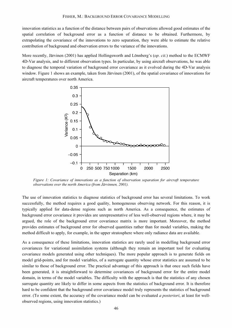
innovation statistics as a function of the distance between pairs of observations allowed good estimates of the spatial correlation of background error as a function of distance to be obtained. Furthermore, by extrapolating the covariance of the innovations to zero separation, they were able to estimate the relative contribution of background and observation errors to the variance of the innovations.

More recently, Järvinen (2001) has applied Hollingsworth and Lönnberg’s (op. cit.) method to the ECMWF 4D-Var analysis, and to different observation types. In particular, by using aircraft observations, he was able to diagnose the temporal variation of background error covariance as it evolved during the 4D-Var analysis window. Figure 1 shows an example, taken from Järvinen (2001), of the spatial covariance of innovations for aircraft temperatures over north America.

Figure 1: Covariance of innovations as a function of observation separation for aircraft temperature observations over the north America (from Järvinnen, 2001).

The use of innovation statistics to diagnose statistics of background error has several limitations. To work successfully, the method requires a good quality, homogeneous observing network. For this reason, it is typically applied for data-dense regions such as north America. As a consequence, the estimates of background error covariance it provides are unrepresentative of less well-observed regions where, it may be argued, the role of the background error covariance matrix is more important. Moreover, the method provides estimates of background error for observed quantities rather than for model variables, making the method difficult to apply, for example, in the upper stratosphere where only radiance data are available.

As a consequence of these limitations, innovation statistics are rarely used in modelling background error covariances for variational assimilation systems (although they remain an important tool for evaluating covariance models generated using other techniques). The more popular approach is to generate fields on model grid-points, and for model variables, of a surrogate quantity whose error statistics are assumed to be similar to those of background error. The practical advantage of this approach is that once such fields have been generated, it is straightforward to determine covariances of background error for the entire model domain, in terms of the model variables. The difficulty with the approach is that the statistics of any chosen surrogate quantity are likely to differ in some aspects from the statistics of background error. It is therefore hard to be confident that the background error covariance model truly represents the statistics of background error. (To some extent, the accuracy of the covariance model can be evaluated a posteriori, at least for well-observed regions, using innovation statistics.)

46


The most popular choice for a surrogate for samples of background error is to use differences between forecasts of different length that verify at the same time. This choice is frequently referred to as the NMC method, after its introduction by Parrish and Derber (1992).

Typically, pairs of forecasts whose lengths differ by 24 hours are used, since this minimizes the chance of aspects of the model’s diurnal cycle being incorrectly interpreted as background errors. The shorter forecast is typically chosen to be at least 12 hours long to reduce the risk of spuriously incorporating “spin up” effects into the diagnosed statistics of background error.

The main advantage of the NMC method is that, in an operational NWP environment, the forecasts required to calculate the statistics are already available in the operational archives. No computationally expensive running of the forecast or analysis system is required. However, the method has several shortcomings. This was already well recognised by Parrish and Derber (op. cit.), who describe the method as “a very crude first step”.

Differences between forecasts of different lengths are produced by the impact of data assimilation in the period between the starting times of the two forecasts. In poorly-observed regions, there may be few observations to effect a change in the initial condition of the later forecast, with the result that the two forecasts will be very similar. It is therefore likely that the NMC method underestimates the variance of background error in data-sparse regions. A second problem arises due to the length of the forecasts, which are typically between 12 and 48 hours. This is significantly longer than the forecast used to generate the background fields. As a result, covariances of forecast differences are likely to be broader in the horizontal and the vertical than those of background error.

The NMC method was used to construct the background error statistics used in the ECMWF variational analysis before October 1999. Since then, an alternative method has been used, in which statistics of background error are estimated from an ensemble of analyses. This method is described below.

3. Estimating Background Error Statistics from Ensembles of Analyses

Suppose we perturb all the inputs to the analysis system. The result will be a perturbed analysis. Moreover, if the perturbations are drawn from the distributions of the true random errors in the inputs, the resulting analysis will be perturbed by an amount drawn from the distribution of analysis error. To see that this is the case, consider that the inputs to an unperturbed analysis may be regarded as being produced by adding perturbations, drawn from the relevant error distributions, to the true values of the input quantities. By definition, the analysis in this case differs from the truth by an amount equal to the analysis error.

Suppose now that a short forecast is run from the perturbed analysis, such as is required to produce the background field for a subsequent analysis. The result will be a perturbed forecast. Furthermore, neglecting the effects of model error, the perturbation to the forecast will have the statistical characteristics of short-term forecast (i.e. background) error. (The effect of model error may be incorporated by adding a stochastic forcing term to the model equations.) The idea is show schematically in Figure 2.

Analysisxb+εb

y+εo

SST+εSST (etc.)

xa+εaForecast

xf+εfAnalysis

xb+εb

y+εo

SST+εSST (etc.)

xa+εaForecast

xf+εf

Figure 2: Schematic illustration showing how a perturbed analysis and forecast may be generated by perturbing the inputs to the analysis system.

47


If now we run a new cycle of analysis with perturbed inputs, we may use the perturbed forecast to provide it with perturbed background fields. This allows a second perturbed analysis and forecast to be produced without requiring us explicitly to specify new perturbations to the background. This process may be continued for many analysis cycles. Furthermore, after a few days, the statistical characteristics of the perturbations of the analysis and forecast fields will depend only weakly on the initial background perturbation, so that a sequence of background fields may be generated whose statistical characteristics are essentially independent of the initial background perturbation.

By running the analysis-forecast system twice for the same period, and by perturbing both runs using statistically independent perturbations drawn from the relevant distributions, we may generate pairs of contemporaneous perturbed background fields. The differences between these pairs of background fields have the statistical characteristics of differences between fields of background error. That is, they have the correlation structure of background error but twice the variance. The method is illustrated in Figure 3.

Background differences

Analysis Forecastxb+εb



Analysis Forecastxb+ηb



Background differences




















Figure 3: Schematic illustration of the analysis-ensemble method of generating fields of background difference.

This method of generating surrogate fields of background error clearly has much in common with the ensemble Kalman filter (e.g. Evensen, 2003). The possibility of exploiting this connection to provide a flow-dependent background error covariance model is clearly attractive. However, we have yet to explore this avenue, and have so far restricted our attention to generating coefficients for the current ECMWF static covariance model.

In common with the NMC method, the analysis-ensemble method produces global fields of model variables on the model grid. This is a significant advantage over methods based on innovation statistics. Unlike the NMC method, however, we can expect reasonable estimates to be produced of the variance of background error in data-sparse regions. This is because any small difference in the initial state will amplify over several analysis cycles, eventually reaching the level implied by climatological variance, unless checked by the incorporation of observational information.

The analysis ensemble method may be regarded as a diagnostic of the actual statistical characteristics of the analysis system to which it is applied. This is both an advantage and a disadvantage. It is clearly useful to be able to diagnose the characteristics of the analysis system. However, the method does not necessarily produce the optimum covariance matrix of background error for a given system. As a simple example, suppose that the analysis system tends to produce analyses that have excessive levels of gravity-wave activity. The analysis ensemble method will correctly diagnose a large variance for gravity-wave modes in the background errors. If now a new background error covariance model is generated from the diagnosed statistics, and used in the analysis system, it will assign large variances to gravity wave modes. The resulting

48


analyses are likely to contain even larger levels of gravity-wave noise than were produced using the original background error covariance model.

A particular advantage for the analysis ensemble method is that it estimates statistics for forecasts of the same length as are used to provide the background fields for the analysis. By contrast, forecasts used to derive statistics by the NMC method are typically significantly longer than those used to provide background fields. The effect of forecast length on the structure of background error correlation was shown by Järvinen (2001), and can also be illustrated using the analysis ensemble method by running forecast from the perturbed analyses and calculating statistics of forecast difference for different forecast lengths. This is illustrated in Figure 4, which shows the difference between the estimated correlation of forecast error and that of analysis error for 500hPa geopotential as a function of distance, and for various forecast lengths.

Figure 4: The difference between forecast correlation and analysis correlation calculated using the analysis ensemble method for 500hPa geopotential, and for a selection of forecast ranges.

It is clear that forecast correlations tend to increase with time at distances less than about 1200km, and to decrease with time for longer distances.

Figure 5 shows a comparison of background error correlation for 500hPa geopotential calculated using the NMC and analysis-ensemble methods. The difference is consistent with the view that the NMC method tends to produce correlations that are representative of longer forecasts than those used to generate background fields for the analysis.

49


Figure 5: Background error correlation for 500hPa geopotential estimated using the NMC method (solid line) and the analysis ensemble method (dashed line).

The analysis ensemble method also tends to produce correlations that are shallower than those generated using the NMC method. Figure 6 and Figure 7 show vertical correlations of vorticity calculated using the two methods.

Figure 6: Mean vertical correlation for vorticity as a function of model level, calculated using the analysis-ensemble method.

Figure 7: Mean vertical correlations for vorticity calculated using the NMC method.

4. Modelling of Background Error Statistics Using Spectral Methods

The state vector of a typical analysis system for NWP has a dimension of around 106. Consequently, the background error covariance matrix contains roughly 1012 elements. This is too large to be stored in the memory of current computers. Moreover, to specify the elements of such a matrix, we require at least 106 background or forecast differences. This is far more than are available. It is therefore necessary to reduce the

50


problem to manageable proportions by constructing the background covariance matrix from a set of very sparse matrices. In the ECMWF variational analysis system, the background error covariance matrix is given by

(1) T T=B L Σ CΣL

Here, L is a balance operator that accounts for correlations between the mass field (i.e. temperature and surface pressure) and the wind field. This matrix is sparse. The matrix Σ is implemented as an inverse spectral transform from the spectral coefficients of the model state vector, followed by a multiplication at each gridpoint by the standard deviation of background error, followed by a spectral transform. These operations are also sparse. Finally, the matrix C is block diagonal, with one block for each total wavenumber n, and for each variable. Each block has dimension Nlevels×Nlevels, where Nlevels is the number of model levels.

The diagonal blocks of C are each of the form

(2) n nh V

where Vn is a correlation matrix, and represents the vertical correlation for a particular variable and wavenumber. By specifying different vertical correlation matrices for different wavenumbers, it is possible to produce vertical correlations that depend on horizontal scale, so that features with large horizontal scale have deeper vertical correlations than features of small horizontal scale. This non-separability of vertical and horizontal correlations is necessary for the simultaneously-correct specification of mass and wind correlations (Phillips, 1986; Bartello and Mitchell, 1992).

The coefficients hn in equation (2) determine the horizontal correlation. This representation of the horizontal correlations defines the horizontal correlation matrix as equivalent to a convolution on the sphere with a function of great-circle distance. Specifically, the convolution of a function f defined on the sphere with a function h of great circle distance is given by

, ,,

( , )n m n m nm n

h f h f Y λ φ⊗ =∑ (3)

where the coefficients hn are the coefficients of the Legendre transform of h.

The advantage of this spectral approach is that it reduces the horizontal correlation matrix to a diagonal matrix. The disadvantage is that, by assuming the correlations to be equivalent to a convolution, the resulting correlations are homogeneous and isotropic. This is clearly a major shortcoming of the method. Nevertheless, the spectral method remains attractive due to its efficiency, the ease with which its coefficients may be calculated from forecast or background differences, and its absence from polar discontinuities. Fortunately, it is possible to relax the restrictions of homogeneity and isotropy while retaining the advantages of the spectral approach.

A method for including anisotropy in a spectral covariance model was presented by Dee and Gaspari (1996). They showed that an anisotropic covariance model may be produced by adopting a three-step process. In the first step, a horizontal coordinate transform is applied, so that functions specified on a grid represented by the points xi are interpolated to a new grid represented by the points Xi. The coordinate X is related to the coordinate x by a given invertible functional relationship, X=g(x).

The second step of the covariance model is to apply an isotropic covariance model in the transformed coordinate, X. This may be implemented as a spectral convolution. Finally, the convolved fields are

51


interpolated back to the original grid defined by the points xi. Although the covariance model is isotropic with respect to the X coordinate, it is anisotropic with respect to the x coordinate.

Dee and Gaspari (op. cit.) chose g to be a simple function of latitude. The resulting correlations were elongated with respect to a purely isotropic covariance model along the north-south axis in mid-latitudes, and along the east-west direction in the tropics. A more general coordinate transformation, based on momentum coordinates, was used by Desroziers (1997).

Vertical coordinate transformations may also be useful in defining background covariance models. It is clear that there are three distinct regions for which vertical correlations have different characteristics. These regions are the boundary layer, the free troposphere and the stratosphere. In the current ECMWF covariance model, these regions are identified only approximately, by fixed model levels. It is likely that the specification of vertical correlation could be significantly improved by employing a vertical coordinate transform that explicitly maps the transitions between these regions onto fixed surfaces of the coordinate system. One possibility might be to use a boundary-layer variant of the coordinate introduced by Zhu et al. (1992):

( )

1 2 1 21

1 2 1 2 1 2

1/ 2

*

for

otherwiseB

B

k k BB

k k k

k k KN K

BB

a b pk K

c T dp

ppp

κ

+ +

−

+ + +

+ −−

+<

+=

(4)

Here, *p is surface pressure, Bp is the pressure at the top of the boundary layer, and Tk+1/2 is the

temperature.

Figure 8: A possible vertical coordinate for use in a background covariance model.

52


This coordinate system has exactly KB levels evenly spaced in log-pressure in the boundary layer. For appropriate choices of the coefficients ak+1/2, bk+1/2 and ck+1/2, the coordinate tends to an isentropic vertical coordinate in the lower stratosphere. The coordinate system is illustrated in Figure 8 for an idealised case. The coordinate marked in red coincides with the top of the boundary layer, and the first fully-isentropic surface is marked in blue.

5. Including Inhomogeneity in the Spectral Method

The spectral approach to covariance modelling described above has the major disadvantage that the correlations it produces are spatially homogeneous. In effect, the method provides full resolution of the variation of vertical and horizontal correlation as a function of total wavenumber n, but provides no spatial resolution: a single correlation model is applied at all points on the sphere.

At the opposite end of the spectrum, it is possible to specify vertical and horizontal correlations in the grid-space of the model, as a function of horizontal location. This approach allows full spatial resolution, but provides no spectral resolution. In particular, with this approach, the same vertical correlation matrix is applied, regardless of the horizontal scale of the features involved. As mentioned above, this separability of vertical and horizontal correlations makes it impossible to specify simultaneously correct correlation structures for mass and for wind (Phillips, 1986; Bartello and Mitchell, 1992).

Clearly, a compromise between the two extremes of spatial and spectral resolution is required. It is well know that wavelet methods allow simultaneous resolution of spatial and spectral features, making them attractive for use in background covariance modelling. Tangborn and Zhang (2000) demonstrated the use of wavelets to provide a basis for the propagation of covariances in a low-rank approximate Kalman filter. Their model had a rectangular domain, for which it was straightforward to define an orthogonal wavelet basis. The definition of a wavelet basis for the sphere is less trivial.

There have been several attempts to define orthogonal wavelets on the sphere. Schröder and Sweldens (1995) defined wavelets based on an underlying triangulation of the sphere. Goettlemann (1996) and Schaffrin et al. (2002) used latitude-longitude grids with varying zonal resolution. Both approaches result in complete orthogonal, or bi-orthogonal, bases for the sphere. However, with these bases, it is not possible to define finite truncations that are free from special points. That is, given a function represented by a finite set of non-zero coefficients, arbitrary rotations of the function on the sphere cannot be represented using the same finite basis. In practice, this means that a covariance model constructed using these bases will inevitably suffer from some form of discontinuous behaviour at the special points.

An alternative method for constructing wavelets on the sphere was suggested by Freeden and Windheuser (1996). They defined wavelets in terms of convolutions with radial basis functions (i.e. functions of great circle distance, r). Such wavelets are free from special points, but are non-orthogonal. The lack of special points, and the close connection between the construction of wavelets using convolutions and the convolution-based approach used in the current ECMWF background covariance model, makes Freeden and Windheuser’s approach attractive for use in constructing a covariance model.

A finite, non-orthogonal wavelet transform on the sphere is defined by a set of radial basis functions

{ }( ) ; 1j r j Kψ = … with the property:

(5) 2max

1

ˆ ( ) 1 for 0K

jj

n nψ=

= = …∑ n

53


where ˆ ( )j nψ is the nth coefficient of the Legendre transform of ψ, and where ˆ ( ) 0j nψ = for n>nmax. (Note

that we have restricted our attention to a finite set of functions with finite series of Legendre coefficients. This restriction is not necessary for the theory to apply. It is assumed for convenience.)

Consider a function f on the sphere whose spectral coefficients are zero for n>nmax. We define the wavelet “coefficients” to be the functions defined by convolving f with each of the radial basis functions:

for 1j jf f j Kψ= ⊗ = … (6)

Now consider the sum:1

K

jj

jfψ=

⊗∑ . Considering the (m,n)th spectral component of the spherical harmonic

expansion of this sum, we have:

(7)

( ).1 1

,

2,

1

,

ˆˆ ( )

ˆˆ ( )

ˆ

K K

j j j j m nj jm n

K

j m nj

m n

f n

n f

f

ψ ψ

ψ

= =

=

⊗ =

=

=

∑ ∑

∑

f

j

The last step in equation (7) is derived using equation (5). We may write equation (7) as:

jj

f fψ= ⊗∑ (8)

Equations (6) and (7) form a sort of transform pair (strictly, a “resolution of the identity”). They show that the functions ( )rjψ form a particular mathematical construct known as a “tight frame” (see, for example,

Daubechies, 1992). The existence of a transform pair is the crucial property that makes the wavelet basis useful. Specifically, we choose the functions ( )rjψ to be both spatially localised, and restricted to a band of

wavenumbers, n. We can then regard the value of the function fj at a given location on the sphere as representing local features of the function f that have a horizontal scale corresponding to the selected band of wavenumbers. Equation (8) shows that if we manipulate the functions fj, then the results of these manipulations will produce spatially and spectrally localised effects on the corresponding function on the sphere.

Freeden and Windheuser (op. cit.) generated spherical wavelets using a family of radial basis functions ( )j rψ , derived from a single generator function. This has advantages when considering infinite expansions

in wavelets on the sphere as it simplifies the mathematics. However, for finite expansions, there is no particular advantage to using a single generator function. Instead, we choose to define a set of spectrally band-limited functions, ( )j rψ , whose Legendre transforms satisfy:

1ˆ ( ) 0 if or j jn n N n 1jNψ − += < > (9)

for some series of cut-off wavenumbers N1...NK. For example, we could choose:

54


12

11

1

12

11

1

ˆ ( ) for

ˆ ( ) for

ˆ ( ) 0 otherwise.

jj j

j j

jj

j j

j

n Nn N

N N

N nn N

N N

n

ψ

ψ

ψ

−−

−

+

j

j j

n N

n N ++

−= < −

−= − =

≤

< < (10)

Figure 9 shows the spectral coefficents for the functions defined by equation (10). The corresponding functions of great-circle distance are shown in Figure 10. (Note that, for clarity, the functions have been offset along the vertical axis.) It is clear that, for practical purposes, the functions are spatially localised, with functions corresponding to higher bands of wavenumbers having smaller spatial extent than those corresponding to low bands of wavenumbers.

0 10 20 30 40 50 60 70 80 90 100 110 120 130 140 150

Wavenumber n

0

0.2

0.4

0.6

0.8

1

Wavelet functions: ψ̂j(n) = ( φ̂2j(n) - φ̂2

j-1(n) )1/2

Figure 9: Spectral coefficients of the wavelet functions defined by equation (10).

0 500 1000 1500 2000 2500 3000 3500 4000 4500 5000

great-circle distance (km)

Wavelet functions: ψj(|r|)

Figure 10: Functions of great-circle distance corresponding to the functions shown in Figure 9.

55


In a variational analysis system, it is usual to define the background covariance matrix implicitly by introducing a new variable, χ, related to the background departure through ( )b− =x x Lχ . The background

cost function is then:

T12bJ = χ χ (11)

The background error covariance implied by this change of variable is B=LLT. Note in particular that it is not necessary for L to be invertible, or even square.

To define a wavelet-based background covariance model, we define the control vector such that

( )T T T T1 2, , , K=χ χ χ χ… , where:

( )1 2 1 2( , ) ( )j j j b bλ φ ψ− −= ⊗ −χ C Σ T x x (12)

Here, Σb is the matrix representing the gridpoint variances of background error, and T is the matrix representing the balance operator (see the next section of this paper, and also Derber and Bouttier, 1999). These matrices are retained from the current specification of the ECMWF analysis control variable.

The matrix ( , )j λ ϕC is a vertical covariance matrix. In principle, one such matrix may be specified at each

grid-point of the spatial representation of 1 2 (j b bψ −⊗ −Σ T x x ) . In practice, it may be necessary to reduce

the number of matrices to be specified, for example by using the same matrix for several gridpoints.

The dimension of the control vector is larger than that of the background departure. As noted above, this does not matter for the definition of the background error covariance matrix. From the practical point of view, we note that each of the functions χj is band limited (assuming that the horizontal variation of the covariance matrices is also band-limited). Each may be represented exactly on a Gaussian grid of appropriate resolution. Functions corresponding to the largest scales can be represented on coarse grids, so that the total dimension of the control vector need not be excessive.

Using equation (8), we may derive an expression for the background departure as a function of the control vector:

1 1 2 1 2 ( , )b b j jj

ψ λ φ−j − = ⊗ ∑x x T Σ C χ (13)

This is of the form ( )b− =x x Lχ , so that the implied background covariance matrix is B=LLT.

It is clear from equation (13) that the background departure at a given location is determined by the sum of convolutions of the functions ( , )j jλ ϕC χ with the functions ψj. Each convolution corresponds to a local

averaging of nearby values, by virtue of the spatial localisation of the wavelet functions. Consequently, only the covariance matrices Cj(λ,φ) corresponding to nearby points have an influence in determining the background departure at a given location. By allowing the covariance matrices to vary with latitude and longitude, we achieve spatial variation of the covariances.

To understand the spectral properties of the covariances implied by equation (13), consider the special case in which the covariance matrices Cj(λ,φ) are independent of latitude and longitude. In this case, the multiplication commutes with the convolution, and we have:

56


( )1/ 2 1 2b b b j j

j

σ ψ− − = ⊗ j∑Σ T x x C χ (14)

Taking the spectral transform, we find that the matrix L that defines the change of variable has spectral representation

( )1 1/ 2 1/ 2 1/ 2 1/ 21 1 2 2

ˆ ˆ ˆ, , ,b−=L T Σ C Ψ C Ψ C Ψ… K K (15)

where is the diagonal matrix of coefficients ˆjΨ ˆ ( )j nψ . For a given wavenumber, n, the implied covariance

matrix for the variable is: ( )1/ 2b b− −Σ T x x

(16) 2

1

ˆ ( )K

jj

nψ=∑ C j

Now, from equation (5), we have 2ˆ ( ) 1jj

nψ =∑ . Hence, equation (16) represents an interpolation in

wavenumber of the matrices Cj. For the particular functions defined in equation (10), the interpolation is piecewise linear. Hence we see that, for the special case of spatially invariant covariance matrices, the wavelet Jb is equivalent to a version of the current formulation of the ECMWF covariance model in which the vertical correlation matrices, Vn, and the coefficients defining the horizontal structure functions, hn, are piecewise linear functions of wavenumber n.

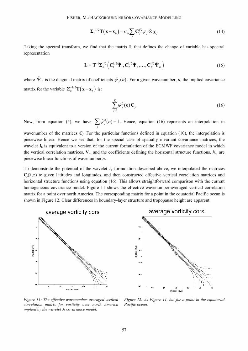
To demonstrate the potential of the wavelet Jb formulation described above, we interpolated the matrices Cj(λ,φ) to given latitudes and longitudes, and then constructed effective vertical correlation matrices and horizontal structure functions using equation (16). This allows straightforward comparison with the current homogeneous covariance model. Figure 11 shows the effective wavenumber-averaged vertical correlation matrix for a point over north America. The corresponding matrix for a point in the equatorial Pacific ocean is shown in Figure 12. Clear differences in boundary-layer structure and tropopause height are apparent.

Figure 11: The effective wavenumber-averaged vertical correlation matrix for vorticity over north America implied by the wavelet Jb covariance model.

Figure 12: As Figure 11, but for a point in the equatorial Pacific ocean.

57


The ability of the wavelet Jb formulation to produce inhomogeneous horizontal correlations is demonstrated in Figure 13, which shows the effective horizontal structure functions for points over north America and over the equatorial Pacific. The length scale for horizontal correlation is clearly larger in the equatorial Pacific than over north America.

Figure 13: Effective horizontal structure functions for vorticity for a point over north America and a point in the equatorial Pacific.

6. Incorporating Flow-Dependent Dynamical Balance in the Background Covariance Model

Derber and Bouttier (1999) showed that an effective multivariate covariance model for a variational analysis could be produced by applying a univariate covariance model to suitably transformed model variables. Specifically, restricting attention to vorticity, divergence, surface pressure and temperature, they applied a

univariate covariance model to the variables ( )( ), , ,bal u s uuD p Tζ , defined as:

( )( )

( )

( )( ) ( )

( ) ( ) ( ) ( )( )

bal

bal balu

bal bal div uu

s s bal bal s div us u

D D PDT T P T DTp p P p Dp

ζζζζ

ζ

=−=− −=− −=

(17)

Here, Pbal is a pseudo-geopotential, determined by a statistical regression between spectral coefficients of vorticity and geopotential. Dbal, Tbal and (ps)bal are determined by statistical regressions with Pbal, and Tdiv and (ps)div are determined by statistical regression with Du.

The change of variable defined by equation (17) is invertible. For example, for temperature, we have:

( )( ) ( )u bal bal div uT T T P T Dζ= + + (18)

58


Now, since Tu, ζ and Du are assumed to be uncorrelated, the covariance matrix for temperature is given by the sum of the covariance matrices for Tu, Tbal and Tdiv. The covariances for the latter two variables are determined by the action of the assumed functional (balance) relationship between Tbal and vorticity, and between Tdiv and Du, on the covariance matrices for vorticity and for Du.

Derber and Bouttier (op. cit.) defined Pbal using linear regression. However, they restricted the regression matrix to be tri-diagonal with respect to the spherical harmonic representations of the vorticity and geopotential fields. The coefficients they derived through regression were, in fact, highly similar to those of the corresponding linear balance equation, so that use of analytical linear balance rather than regression would make little difference to the implied covariance model. Given this fact, it is interesting to ask whether alternative analytical expressions, which are more accurate than linear balance, might be of use in the covariance model.

A particular improvement over the linear balance equation is provided by the non-linear balance equation (see, for example, Haltiner and Williams, 1980). This defines a balanced geopotential as:

( )2 . .balP ψ ψ ψ∇ = −∇ ∇ + ×v v k vf (19)

Here, vψ denotes the rotational wind. The nonlinear balance equation is equivalent to the linear balance equation in the case that the rotational wind is everywhere orthogonal to its gradient. It is equivalent to gradient wind balance for circular flow. The nonlinear term in equation (19) becomes important in regions of strong acceleration or curvature. As such, it is expected that use of the nonlinear balance equation in the covariance model should result in improved analyses in dynamically active regions, such as jet entrances and exits.

Derber and Bouttier’s formulation includes a regression between divergence and Pbal. The effect of this regression is to produce inflow into surface cyclonic flow, and corresponding outflow aloft. It is possible to augment this simple relationship with analytical expressions for the balanced divergence. One possibility is to use the quasi-geostrophic omega equation:

2

2 20 2( )f

pσ ω∂∇ + = − ∇

∂Q2 . (20)

Here, we use the Q-vector form of the omega equation (Hoskins et al., 1978). As with the nonlinear balance equation, we expect the use of the quasi-geostrophic omega equation to improve the covariance model in dynamically active regions.

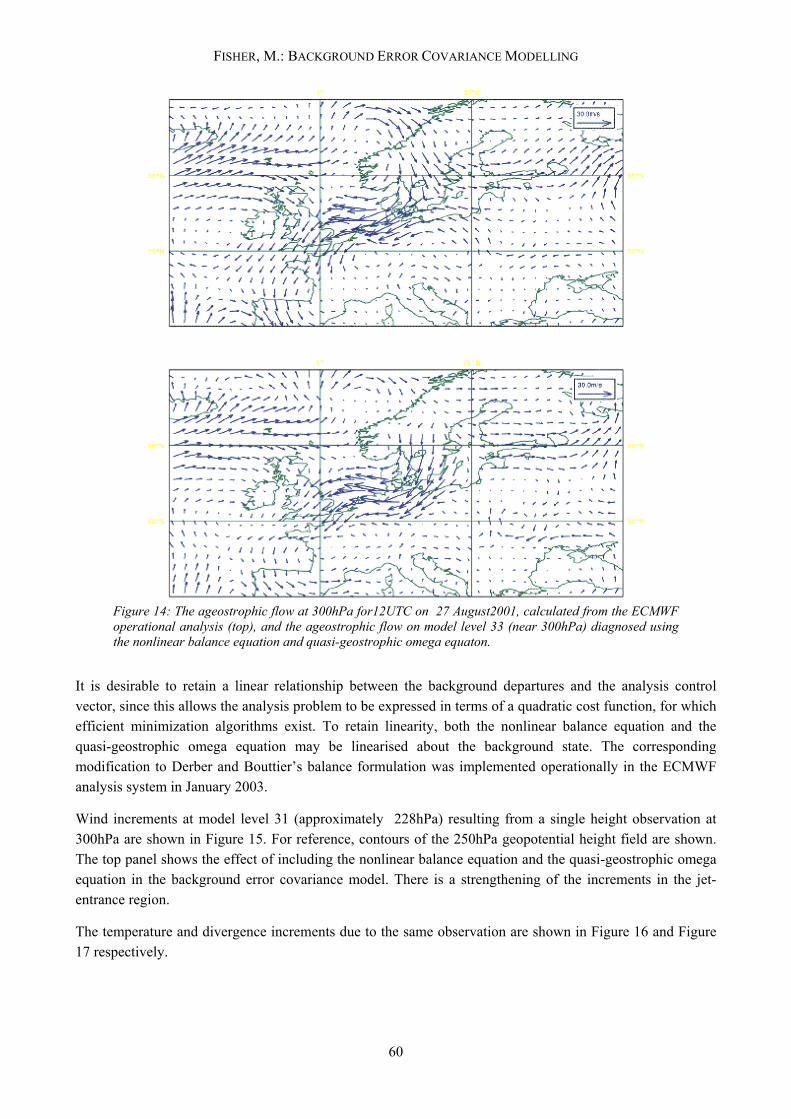
Figure 14 shows the ageostrophic flow at 300hPa for 12UTC on 27 August 2001 calculated from the ECMWF operational analysis, together with the ageostrophic flow on a nearby model level, diagnosed using the nonlinear balance equation and quasi-geostrophic omega equation. The resemblance between the two plots is striking.

59


Figure 14: The ageostrophic flow at 300hPa for12UTC on 27 August2001, calculated from the ECMWF operational analysis (top), and the ageostrophic flow on model level 33 (near 300hPa) diagnosed using the nonlinear balance equation and quasi-geostrophic omega equaton.

It is desirable to retain a linear relationship between the background departures and the analysis control vector, since this allows the analysis problem to be expressed in terms of a quadratic cost function, for which efficient minimization algorithms exist. To retain linearity, both the nonlinear balance equation and the quasi-geostrophic omega equation may be linearised about the background state. The corresponding modification to Derber and Bouttier’s balance formulation was implemented operationally in the ECMWF analysis system in January 2003.

Wind increments at model level 31 (approximately 228hPa) resulting from a single height observation at 300hPa are shown in Figure 15. For reference, contours of the 250hPa geopotential height field are shown. The top panel shows the effect of including the nonlinear balance equation and the quasi-geostrophic omega equation in the background error covariance model. There is a strengthening of the increments in the jet-entrance region.

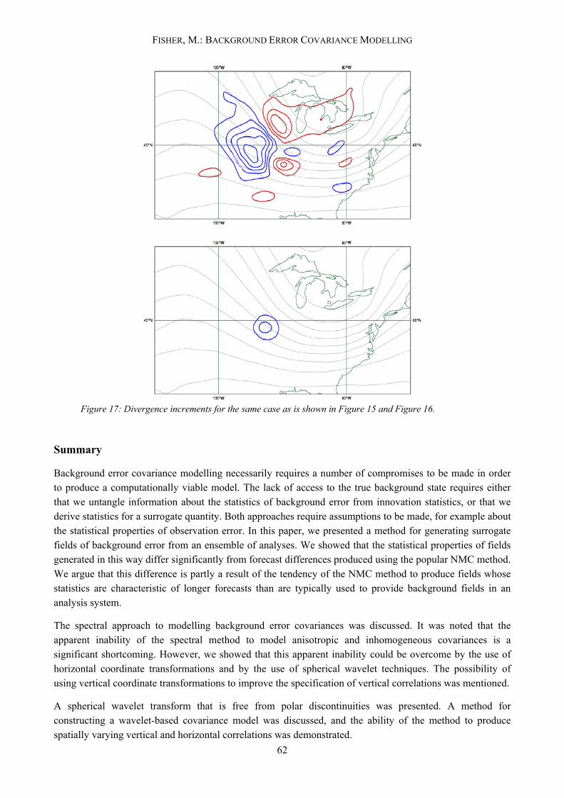
The temperature and divergence increments due to the same observation are shown in Figure 16 and Figure 17 respectively.

60


Figure 15: Wind increments on model level 31 (near 228hPa) resulting from a single height observation at 300hPa. Top panel: balance operator includes linearizations about the background of the nonlinear balance equation and the quasi-geostrophic omega equation. Bottom panel: Derber and Bouttier’s (1999) balance operator.

Figure 16: Temperature increments for the same case as is shown in Figure 15.

61


Figure 17: Divergence increments for the same case as is shown in Figure 15 and Figure 16.

Summary

Background error covariance modelling necessarily requires a number of compromises to be made in order to produce a computationally viable model. The lack of access to the true background state requires either that we untangle information about the statistics of background error from innovation statistics, or that we derive statistics for a surrogate quantity. Both approaches require assumptions to be made, for example about the statistical properties of observation error. In this paper, we presented a method for generating surrogate fields of background error from an ensemble of analyses. We showed that the statistical properties of fields generated in this way differ significantly from forecast differences produced using the popular NMC method. We argue that this difference is partly a result of the tendency of the NMC method to produce fields whose statistics are characteristic of longer forecasts than are typically used to provide background fields in an analysis system.

The spectral approach to modelling background error covariances was discussed. It was noted that the apparent inability of the spectral method to model anisotropic and inhomogeneous covariances is a significant shortcoming. However, we showed that this apparent inability could be overcome by the use of horizontal coordinate transformations and by the use of spherical wavelet techniques. The possibility of using vertical coordinate transformations to improve the specification of vertical correlations was mentioned.

A spherical wavelet transform that is free from polar discontinuities was presented. A method for constructing a wavelet-based covariance model was discussed, and the ability of the method to produce spatially varying vertical and horizontal correlations was demonstrated.

62


63

Finally, the possibility of including non-linear, analytical balances in the covariance model was demonstrated.

References

Bartello, P. and H.L. Mitchell, 1992: A continuous three-dimensional model of short-range forecast error covariances, Tellus 44A, 217-235.

Daubechies, I., 1992: Ten Lectures on Wavelets. CBMS-NSF regional conference series in applied mathematics, SIAM.

Dee, D.P. and G. Gaspari, 1996: Development of anisotropic correlation models for atmospheric data assimilation. Preprint volume, 11th Conf. on Numerical Weather Prediction, August 19-23, 1996, Norfolk, VA, pp 249-251.

Derber, J. and F. Bouttier, 1999: A reformulation of the background error covariance in the ECMWF global data assimilation system. Tellus, 51A, 195-221.

Desroziers, G., 1997: A coordinate change for data assimilation in spherical geometry of frontal surfaces. Mo. Wea. Rev., 125, 3030-3038.

Evensen, G., 2003: The ensemble Kalman filter: theoretical formulation and practical implementation. Ocean Dynamics (in print).

Freeden, W. and U. Windheuser, 1996: Spherical wavelet transform and its discretization. Adv. Comput. Math. 5, 51-94.

Goettelmann, J, 1996: Locally Supported Wavelets on the Sphere. Technical report, Department of Mathematics, University of Mainz, Germany.

Hoskins B.J., I. Draghici and H.C. Davies, 1978: A new look at the ω-equation. Quart. J. Roy. Met. Soc., 104, 31-38.

Hollingsworth, A., and P. Lonnberg, 1986: The statistical structure of short-range forecast errors as determined from radiosonde data. Part I: The wind field. Tellus, 38A, 111-136.

Järvinen, H., 2001: Temporal evolution of innovation and residual statistics in the ECMWF variational data assimilation systems. Tellus, 53A, 333-347.

Parrish and Derber , 1992: The national meteorological center’s spectral statistical-interpolation analysis system. Mon. Wea. Rev., 120, 1747-1763.

Phillips, N.A., 1986: The spatial statistics of random geostrophic modes and first-guess errors. Tellus, 38A, 314-332.

Schraffrin, B., R. Mautz, C. Schum, H. Tseng, 2002: Towards a spherical pseudo-wavelet basis for geodetic applications. Computer-aided civil and infrastructure engineering.

Schröder P. and W. Sweldens, 1995: Spherical wavelets: efficiently representing functions on the sphere. Computer Graphics, Annual Conference Series (Siggraph'95 Proceedings), pp. 161-172, http://citeseer.nj.nec.com/schroder95spherical.html

Tangborn, A. and S.Q. Zhang, 2000: Wavelet transform adapted to an approximate Kalman filter system. Applied Numerical Mathematics, 33, 307-316.

Zhu Z., Thuburn J. and Hoskins B.J. 1992, A vertical finite-difference scheme based on a hybrid σ-θ-p coordinate. Monthly Weather Review, 120, pp851-862.

background error covariance modelling

Documents