1

TRAJECTORY ERROR AND COVARIANCE REALISM FOR LAUNCH COLA OPERATIONS

M.D. Hejduk,* D. Plakalovic,† L.K. Newman,‡ J.C. Ollivierre,§ M.A. Hametz,** B.A. Beaver,†† R.C. Thompson‡‡

Non-uniform guidance and practices for launch collision avoidance

(LCOLA) among different NASA field centers (and the Air Force launch rang-

es) has prompted NASA Headquarters to commission a study to develop rec-

ommendations for standardizing the process and to issue suggested screening

thresholds. The full study should be completed in early 2013, but the results for

the initial phases are reported herein, namely an investigation of the accuracies

of the pre-launch predicted trajectories and the realism of their associated covar-

iances. The study determined that, for the Atlas V and Delta II launch vehicles,

trajectory errors remain about an order of magnitude larger than General Pertur-

bations (GP) satellite catalogue errors, confirming that it is not necessary to re-

sort to a precision catalogue in order to perform LCOLA screenings. The asso-

ciated launch covariances, which are large and had been thought to be conserva-

tively sized, were found instead to be quite appropriately determined and fare

well in covariance realism analyses. As such, the launch-related information

feeding the LCOLA process will allow a durable calculation of the probability

of collision and thus can serve as a reliable basis for LCOLA operations.

INTRODUCTION

While Launch Collision Avoidance (LCOLA) has been a standard launch range practice at

some level for more than a decade, at present there is neither a requirement nor standardized pro-

cess for LCOLA across the Agency. NASA’s Launch Services Program (LSP) for Expendable

Launch Vehicles (ELVs) at NASA Kennedy Space Center (KSC) provides LCOLA analysis to

NASA’s robotic missions if either requested or required by the spacecraft customer. LSP works

with the Aerospace Corporation to perform these functions, as Aerospace also performs similar

functions for Air Force missions. The NASA Human Spaceflight Mission Control Center (MCC)

team has also provided limited pre-launch conjunction screening for the Shuttle. The process is

indeed decentralized, with several different organizations performing calculations and providing

support in different ways.

* a.i. solutions, Inc. 985 Space Center Dr., Suite 205 Colorado Springs, CO 80915 † a.i. solutions, Inc. 985 Space Center Dr., Suite 205 Colorado Springs, CO 80915 ‡ Mail Code 595, NASA Goddard Space Flight Center, 8800 Greenbelt Road Greenbelt, MD 20771 § NASA/KSC address ** NASA/KSC address †† NASA/KSC address ‡‡ Aerospace address

(Preprint) AAS 13-XXX

2

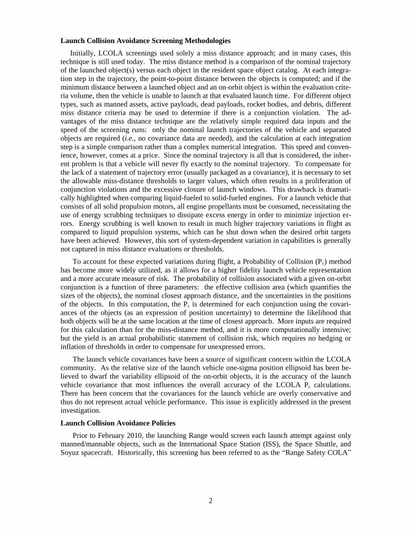
Launch Collision Avoidance Screening Methodologies

Initially, LCOLA screenings used solely a miss distance approach; and in many cases, this

technique is still used today. The miss distance method is a comparison of the nominal trajectory

of the launched object(s) versus each object in the resident space object catalog. At each integra-

tion step in the trajectory, the point-to-point distance between the objects is computed; and if the

minimum distance between a launched object and an on-orbit object is within the evaluation crite-

ria volume, then the vehicle is unable to launch at that evaluated launch time. For different object

types, such as manned assets, active payloads, dead payloads, rocket bodies, and debris, different

miss distance criteria may be used to determine if there is a conjunction violation. The ad-

vantages of the miss distance technique are the relatively simple required data inputs and the

speed of the screening runs: only the nominal launch trajectories of the vehicle and separated

objects are required (i.e., no covariance data are needed), and the calculation at each integration

step is a simple comparison rather than a complex numerical integration. This speed and conven-

ience, however, comes at a price. Since the nominal trajectory is all that is considered, the inher-

ent problem is that a vehicle will never fly exactly to the nominal trajectory. To compensate for

the lack of a statement of trajectory error (usually packaged as a covariance), it is necessary to set

the allowable miss-distance thresholds to larger values, which often results in a proliferation of

conjunction violations and the excessive closure of launch windows. This drawback is dramati-

cally highlighted when comparing liquid-fueled to solid-fueled engines. For a launch vehicle that

consists of all solid propulsion motors, all engine propellants must be consumed, necessitating the

use of energy scrubbing techniques to dissipate excess energy in order to minimize injection er-

rors. Energy scrubbing is well known to result in much higher trajectory variations in flight as

compared to liquid propulsion systems, which can be shut down when the desired orbit targets

have been achieved. However, this sort of system-dependent variation in capabilities is generally

not captured in miss distance evaluations or thresholds.

To account for these expected variations during flight, a Probability of Collision (Pc) method

has become more widely utilized, as it allows for a higher fidelity launch vehicle representation

and a more accurate measure of risk. The probability of collision associated with a given on-orbit

conjunction is a function of three parameters: the effective collision area (which quantifies the

sizes of the objects), the nominal closest approach distance, and the uncertainties in the positions

of the objects. In this computation, the Pc is determined for each conjunction using the covari-

ances of the objects (as an expression of position uncertainty) to determine the likelihood that

both objects will be at the same location at the time of closest approach. More inputs are required

for this calculation than for the miss-distance method, and it is more computationally intensive;

but the yield is an actual probabilistic statement of collision risk, which requires no hedging or

inflation of thresholds in order to compensate for unexpressed errors.

The launch vehicle covariances have been a source of significant concern within the LCOLA

community. As the relative size of the launch vehicle one-sigma position ellipsoid has been be-

lieved to dwarf the variability ellipsoid of the on-orbit objects, it is the accuracy of the launch

vehicle covariance that most influences the overall accuracy of the LCOLA Pc calculations.

There has been concern that the covariances for the launch vehicle are overly conservative and

thus do not represent actual vehicle performance. This issue is explicitly addressed in the present

investigation.

Launch Collision Avoidance Policies

Prior to February 2010, the launching Range would screen each launch attempt against only

manned/mannable objects, such as the International Space Station (ISS), the Space Shuttle, and

Soyuz spacecraft. Historically, this screening has been referred to as the “Range Safety COLA”

3

process. In February 2010, United States Air Force (USAF) instruction AFI 91-217 was enacted,

which mandated operational launch conjunction assessment/collision avoidance screenings by Air

Force-controlled ranges. This AFI continued to require Range Safety COLAs but added LCOLA

screens against on-orbit payloads and debris, this latter addition often called “Mission Assurance

COLA” (MA COLA).

For NASA ELV launches, the Launch Services Program performed an analysis in July 2001

(ELVL-2001-0025354)1 to determine the overall probability that a collision could occur during

the launch phase. Various launch vehicles were examined in different orbit regimes, and the re-

sults indicated that the chance of hitting an on-orbit object during the relatively short launch

phase is so small that Mission Assurance COLA measures have essentially no effect on overall

mission success (It should be noted that at the time of the LSP analysis, the object catalog had

significantly fewer tracked objects than the current catalogue). Following this study, LSP re-

leased a Program Directive (PD) on Collision Avoidance (LSP-PD-120.04), stating that Mission

Assurance COLAs would not be routinely conducted for NASA LSP missions (this directive does

not have any bearing on COLAs conducted by the appropriate launch range for every LSP mis-

sion). However, if LSP’s spacecraft customer requires a MA COLA analysis be performed, LSP

must execute it as a formal mission requirement.

Under this LSP directive, NASA Jet Propulsion Laboratory (JPL) generally does not opt to

perform any LCOLA screenings beyond the Range requirements. For many JPL missions, the

launch window is either a very short duration or instantaneous. Additionally, many planetary or

other deep-space missions have annual or even less frequent launch opportunities. These two

factors combine to magnify the operational impact of standing down due to a low-risk conjunc-

tion.

In contrast, LSP has been conducting MA COLAs for every Goddard Space Flight Center

(GSFC) mission since February 2004. In Goddard Policy RequirementGPR 8000.1, GSFC set

forth the policy that each mission shall perform a MA COLA assessment against all on-orbit ac-

tive satellites; no screening is required against on-orbit debris or spent upper stages. The objec-

tive of the GSFC policy is to protect orbiting assets, not necessarily the payload being launched.

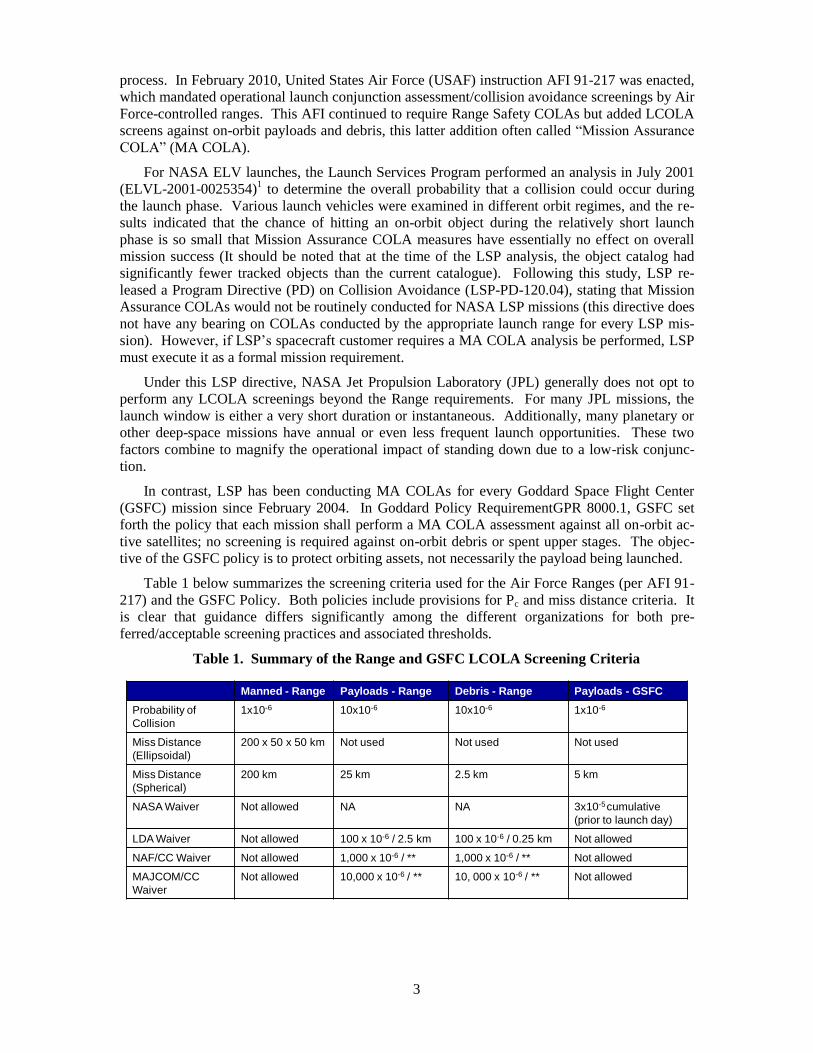
Table 1 below summarizes the screening criteria used for the Air Force Ranges (per AFI 91-

217) and the GSFC Policy. Both policies include provisions for Pc and miss distance criteria. It

is clear that guidance differs significantly among the different organizations for both pre-

ferred/acceptable screening practices and associated thresholds.

Table 1. Summary of the Range and GSFC LCOLA Screening Criteria

Manned - Range Payloads - Range Debris - Range Payloads - GSFC

Probability of

Collision

1x10-6 10x10-6 10x10-6 1x10-6

Miss Distance

(Ellipsoidal)

200 x 50 x 50 km Not used Not used Not used

Miss Distance

(Spherical)

200 km 25 km 2.5 km 5 km

NASA Waiver Not allowed NA NA 3x10-5 cumulative

(prior to launch day)

LDA Waiver Not allowed 100 x 10-6 / 2.5 km 100 x 10-6 / 0.25 km Not allowed

NAF/CC Waiver Not allowed 1,000 x 10-6 / ** 1,000 x 10-6 / ** Not allowed

MAJCOM/CC

Waiver

Not allowed 10,000 x 10-6 / ** 10, 000 x 10-6 / ** Not allowed

4

Launch Collision Avoidance Issues

As the various LCOLA policies and implementation methods illustrate, there are no common-

ly accepted best practices among the agencies. The USAF policy serves to limit orbital debris,

uses the SP catalog, and restricts the use of the Pc method due to their concern about unrealistic

launch vehicle covariances. The GSFC policy serves to be a good steward and protect on-orbit

assets, uses the GP catalog (with covariances estimated from empirical GP error growth infor-

mation), and exclusively uses the Pc method in response to the inherent limitations of the miss

distance method. Furthermore, in cases when similar methods are used, different criteria are em-

ployed with little or no rationale for how the criteria have been established.

While the commissioned NASA study, expected to be fully complete in early 2013, attempts

to address nearly all of these issues, the items addressed in the present paper focus on three foun-

dational issues:

What are the actual errors in pre-launch trajectory estimates for common NASA launch

vehicles?

How do these errors compare to those of on-orbit space objects? What level of space cat-

alogue precision is therefore appropriate for LCOLA screenings?

What is the fidelity of the error statements (covariances) that accompany pre-launch es-

timated trajectories? Can they serve as a reasonable basis for Pc calculations?

The first two bullets above will be addressed in the next section and the final bullet in the section

that follows, after which point certain conclusions will be drawn.

PRE-FLIGHT PREDICTED TRAJECTORY ERRORS

Launch conjunction assessment, as stated in the previous section, is presently only a lightly-

standardized activity in which different indices and launch window closure criteria are used at

different launch agencies and centers. However, regardless of the particular calculation and asso-

ciated window closure approach, the so-called “miss distance,” or the vector magnitude of the

position vector difference between the predicted launch trajectory and a conjuncting object, fig-

ures prominently in the computation; and in some cases this miss distance itself is the parameter

of interest. As such, it is important to gain some understanding of the overall errors in the pre-

dicted launch trajectories, as these errors affect how a miss distance value should be interpreted.

Additionally, the size of these errors will indicate whether analytic orbit models, such as the Sim-

plified General Perturbations Theory #4 (SGP4), are adequate to the calculations for the LCOLA

process or whether high-precision satellite catalogues should be employed.

The launch pre-flight predicted trajectories against which collision avoidance screenings are

run consist of state estimates (position and velocity information) and covariance data at regular

time intervals, typically three-second intervals, with the data beginning from three to thirty se-

conds after launch and continuing until approximately two hours after launch, although the actual

durations are mission-specific. The state estimates are provided in the Earth-Fixed Greenwich

(EFG) coordinate reference frame, primarily for the ease of trajectory adjustment when modifica-

tions to the nominal launch time are required. The furnished covariance information is the lower-

triangle of the position covariance in the UVW (radial, in-track, cross-track) reference frame.

This covariance information is derived from an uncertainty apportionment model that begins with

the expected uncertainty in each of the physical components that govern spacecraft position

5

(thrusters, gyros, &c.) as measured in the laboratory and combines all of these uncertainty data to

synthesize an overall anticipated trajectory uncertainty at each time point. In some sense these

covariance data are provided as a courtesy, as there appears to be no actual “realism” requirement

levied on these error representations. The examination of the realism of these error representa-

tions is addressed in a later section.

The statement of trajectory “truth” against which these pre-flight trajectories can be evaluated

is the actual flight trajectory telemetry data collected during each launch event. These groups of

telemetry data for the missions under analysis were obtained by KSC and converted into a format

convenient for analysis: individual position and velocity measurements of the spacecraft (from

on-board GPS instruments), rendered in the Earth-Centered Inertial (ECI) True-of-Date reference

frame, captured at typically one-second intervals. While this increased data density (increased,

that is, over the three-second intervals in the predicted trajectory data) is certainly welcome, it is

tempered somewhat by frequent data drop-outs. These drop-outs are due to lack of continuous

ground-station coverage and other communications-related difficulties; and while they are more

frequent and severe before TDRSS-enabled communication became more widespread, they re-

main common throughout the five-year period over which trajectories were analyzed.

In comparing the pre-flight trajectories to the associated telemetry in order to determine tra-

jectory errors, a number of issues arise. First, the telemetry data lack any sort of accompanying

error statement, either point-by-point or a single overall value (such as a standard error). In order

to use the data, one is required essentially to presume that the telemetry data represent error-free

truth. One hopes, of course, that the errors in the telemetry data are substantially smaller than

those of the pre-flight trajectories so that the failure to account for the telemetry errors will not

affect results. One will be better able to evaluate the rectitude of this assumption when the actual

sizes of the trajectory errors are determined, as one can form some general opinions about the

expected magnitude of GPS-derived position errors inherent in flight telemetry.

Second, the time points of the pre-flight and telemetry data do not align precisely; so in order

to compare the two datasets some sort of interpolation must be performed. The interpolation of

telemetry points suggests itself as the better choice, as the spacing of the telemetry data is more

frequent and because this approach would eliminate the need to interpolate covariance infor-

mation. Nonetheless, the interpolation of the telemetry still needs to be performed with caution

due to the aforementioned telemetry drop-outs: a simple-minded interpolation scheme that im-

properly attempts to interpolate over non-trivial data-gaps will produce extremely inaccurate re-

sults in such situations. The telemetry interpolation methodology must be robust enough to rec-

ognize such data gaps and avoid them, and the approach adopted here is to require that each of

the two interpolation boundaries be within five seconds of the predicted point. Distances outside

of this range are considered to constitute a data gap and thus are not included in the analysis.

Third, pre-flight telemetry and associated covariance information comes with a particular

predicted launch time. In the majority of the cases the predicted launch time differs from the ac-

tual launch time, the difference between the two launch times is usually small—less than one se-

cond—but it can sometimes be on the order of multiple minutes. The question is whether the ac-

tual or the predicted launch time should be used for accuracy analysis. The actual launch time

scenario represents the trajectory situation as was actually flown, whereas the predicted launch

time represents the situation as was actually screened. The decision was made to use the predicted

launch time, as this situation represents the actual errors that made their way into the screening

process.

As mentioned in the introduction, data were made available and analyzed for thirty-six pre-

launch trajectories, comprising twenty-three Delta II, eleven Atlas V, and two Pegasus trajecto-

6

ries. In some cases partial information was available for other missions, but it is only these thirty-

six that had sufficient, consistent data to merit direct use in the analysis. The launches represent-

ed a considerable variety of orbit types, although both pre-launch trajectory and telemetry data

exist for only the first two to three hours of each event; so all analysis remained within the near-

Earth orbit regime (that region of orbital space for which orbital periods are less than 225

minutes).

Position comparison was made for each point where comparisons were possible; drop-out pe-

riods were simply not analyzed. While it is possible that data dropouts could have systematically

excluded certain levels of trajectory error, the lack of a pattern in the drop-outs’ temporal location

and duration makes this unlikely and suggests the permissibility of straightforward exclusion of

the drop-out periods. Displaying the position difference data as an empirical cumulative distri-

bution function (CDF) curve by individual mission allows the full distribution of the trajectory

errors to be observed and thus more meaningful comparison among different trajectories. Addi-

tionally, the data were filtered by an altitude threshold of 400 km, as there is very little threat of

close approach with space objects at altitudes lower than this (less than 5% of the space catalogue

exists at such low altitudes, and apparently spurious trajectory error data appear at altitudes lower

than this). Figures 1-3 represent the CDF plots of position errors for all three booster types (Atlas

V, Delta II, and Pegasus). The legends spell out the particular missions used, and amplifying in-

formation for each mission is given in the appendix to this paper.

Figure 1 gives the position error results for all Atlas V launches. At the 50th percentile, nearly

all Atlas V launches have errors greater than 10 km; and at the 95th percentile a little under half of

them exceed 100 km.

100

101

102

103

0

10

20

30

40

50

60

70

80

90

100Magnitude of the Position Difference CDF Plot

Cu

mu

lative

Pe

rce

nta

ge

(%

)

Vector Magnitude of Position Difference (km)

AEHF1

DMSP18

JUNO

LRO

MSL

MUOS

SBIRS

SDO

STP1

WGS1

WGS2

Figure 1: CDF plot of trajectory errors for all Atlas V launches

7

100

101

102

103

0

10

20

30

40

50

60

70

80

90

100

Vector Magnitude of Position Difference (km)

Cu

mu

lative

Pe

rce

nta

ge

(%

)

Magnitude of the Position Difference CDF Plot

AQUARIUS

AURA

CALIPSO

COSMO3

GLAST

GPSIIR12

GPSIIR14

GPSIIR15

GPSIIR16

GPSIIR17

GPSIIR18

GPSIIR19

100

101

102

103

104

0

10

20

30

40

50

60

70

80

90

100Magnitude of the Position Difference CDF Plot

Cu

mu

lative

Pe

rce

nta

ge

(%

)

Vector Magnitude of Position Difference (km)

GPSIIR20

GPSIIR21

GRAIL

MITEX

NOAA-N

NOAA-NP

NPP

STEREO

STSS-ATRR

STSS-DEMO

THEMIS

Figures 2a and b: CDF of trajectory errors for Delta II launches

8

Figures 2a and 2b give CDF representations of the position errors for the Delta II launches.

On the whole, these show an error behavior that is somewhat more bounded than for the Atlas V,

although the majority of trajectories show errors above 10 km at the 50th percentile. One trajecto-

ry, that of GPSII Flight 20, shows errors two orders of magnitude greater than all the others; and

further examination was not able to determine any particular cause (e.g., coordinate transfor-

mation problems). Because of its very different error character, this particular trajectory was

judged to be anomalous and not considered in the remainder of the analysis.

Figure 3 represents the CDF plot of the position difference accuracy for Pegasus launches.

There were paired pre-launch trajectory and telemetry data available for only three Pegasus mis-

sions; and all three of these were exceedingly short, with only a few minutes of total data in each.

This is too little data from which to draw any durable conclusions, and as such the Pegasus trajec-

tories are not used in the analyses of the subsequent sections; but as there is some interest in de-

termining whether these solid-fuel motors seem to exhibit the same general error behavior as their

liquid-fuel colleagues, the available data are presented here. The data for one of these trajectories

never exceeded the 400 km altitude threshold and thus are not shown below; for the two others,

what is available is plotted. If this abbreviated sample is truly representative of the entire error

distribution, then one can conclude that the Pegasus error magnitudes and distribution are roughly

similar to those for the Atlas V and Delta II launches.

100

101

102

103

0

10

20

30

40

50

60

70

80

90

100Magnitude of the Position Difference CDF Plot

Cu

mu

lative

Pe

rce

nta

ge

(%

)

Vector Magnitude of Position Difference (km)

AIM

SPACETECH 5

Figure 3: CDF of trajectory errors for Pegasus launches

9

Figures 1-3 give useful presentations of absolute error values and their distributions among

the three different boosters analyzed, but it remains to put these error values in context; and the

natural comparandum is the set of state estimate errors for on-orbit satellites. Such a comparison

will also assist in determining the level of catalogue precision appropriate to the orbital safety

evaluations of these trajectories.

The United States Strategic Command (USSTRATCOM) space catalogue comprises three

distinct sub-catalogues of orbital information. The first is the Special Perturbations (SP) cata-

logue, which uses a higher-order orbital theory to produce a precision set of state estimates; these

data are used internally for JSpOC processes and orbital safety calculations for satellites but are

not generally circulated to external users. The second is the traditional General Perturbations

(GP) catalogue, maintained with SGP4 orbit determination (OD), circulated to external users, and

in recent times posted on www.space-track.org for anyone to download. There is, however, a

new third option that is in beta testing now and is expected to transition within the next year to

maintaining 75% or more of the GP catalogue: the so-called “extrapolation DC,” or in some cir-

cles “eGP.” This approach, described in detail in Cappellucci (2005),2 takes a higher-order

ephemeris (such as those from the SP catalogue) propagated into the future, creates synthesized

observational data (called “pseudo-obs”) from this ephemeris, and executes a GP OD from these

synthesized data. Because the OD is fitting data derived from high-accuracy future predictions,

the quality of the “predictions” using this approach is much better than the traditional, sensor-

observations-based OD. Since the generally-available GP catalogue will be composed of these

two types of GP OD approaches, a comparison of their errors to those of the pre-launch trajecto-

ries can serve both to ground the trajectory errors against some sort of benchmark and at the same

time indicate whether the GP catalogue serves as an adequate basis for LCOLA calculations.

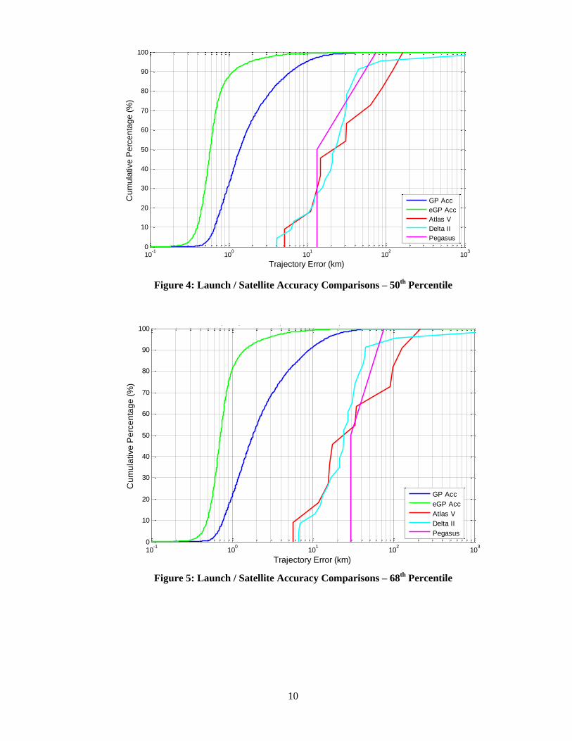
Figures 4-6 compare the errors in the launch trajectories to those of the publically-available

portion of the satellite catalogue. In each of the figures, each CDF line is of a particular accuracy

percentile value: in Figure 4, it is the 50th percentile, in Figure 5 the 68

th percentile, and in Figure

6 the 95th percentile (these percentile values were chosen to remain analogous to the familiar per-

centile values for the mean, one-sigma, and two-sigma levels from a Gaussian distribution, even

though vector error distributions do not in fact follow a Gaussian distribution). Because the con-

struction of the graphic may be somewhat confusing, the following is a step-by-step account of

the features in Figure 4, the 50th percentile accuracy CDF collection. For the Atlas V case, the

50th percentile error value from each of the eleven trajectories was calculated and a CDF curve

constructed of these eleven values (red line); the same was done for the twenty-three Delta II

(green line) and two Pegasus trajectories (pink line). For the satellite catalogue accuracy infor-

mation, the data are derived from an analysis of all GP and eGP data for May 2012; and the 50th

percentile values of a six-hour prediction (roughly equivalent to the amount of propagation used

in LCOLA screenings) errors for each satellite were calculated and also summarized in CDFs.

The precise method of calculating the satellite state estimate accuracies makes use of the refer-

ence orbits calculated for each satellite by the SuperCODAC accuracy estimation program that is

presently part of the Astrodynamics Support Workstation (ASW) operational system; this meth-

odology is described at length in Hejduk, Casali and Ericson (2005)3 and Hejduk (2008).

4

10

10-1

100

101

102

103

0

10

20

30

40

50

60

70

80

90

100Launch Trajectory Errors Compared to Satellite Ephemeris Errors: 50th Percentile

Trajectory Error (km)

Cu

mu

lative

Pe

rce

nta

ge

(%

)

GP Acc

eGP Acc

Atlas V

Delta II

Pegasus

Figure 4: Launch / Satellite Accuracy Comparisons – 50th

Percentile

10-1

100

101

102

103

0

10

20

30

40

50

60

70

80

90

100Launch Trajectory Errors Compared to Satellite Ephemeris Errors: 68th Percentile

Cu

mu

lative

Pe

rce

nta

ge

(%

)

Trajectory Error (km)

GP Acc

eGP Acc

Atlas V

Delta II

Pegasus

Figure 5: Launch / Satellite Accuracy Comparisons – 68th

Percentile

11

10-1

100

101

102

103

0

10

20

30

40

50

60

70

80

90

100Launch Trajectory Errors Compared to Satellite Ephemeris Errors: 95th Percentile

Cu

mu

lative

Pe

rce

nta

ge

(%

)

Trajectory Error (km)

GP Acc

eGP Acc

Atlas V

Delta II

Pegasus

Figure 6: Launch / Satellite Accuracy Comparisons – 95th

Percentile

In the 50th percentile graph (Figure 4), the pre-launch trajectory errors for most of the cumu-

lative percentage span remain about an order of magnitude larger than the GP catalogue errors

and about one and one-half orders of magnitude larger than the eGP errors. In the 68th and 95

th

percentile graphs, the difference is somewhat smaller but still hovers about an order of magnitude

for much of the cumulative percentage span; this is especially so for the eGP data.

There are two conclusions one could draw from these data. First, because the satellite GP

catalogue errors are consistently and substantially smaller than the pre-launch trajectory errors, it

is clear that there will be little to no appreciable benefit from using the precision (SP) rather than

the GP satellite catalogue for LCOLA screenings and risk assessment. It is true that in support of

calculating probabilities of collision, actual OD covariance data generated and preserved with the

precision catalogue can be used, whereas covariances must be estimated when using the GP cata-

logue; but in terms of accuracy levels alone, the inherent errors in the pre-launch trajectories are

so much larger than the GP catalogue errors that if the precision catalogue is not conveniently

available, there is little motivation to take on the difficulties of obtaining and using it for LCOLA.

One could also remark that the trajectory errors are so large in an absolute sense that orbital

safety calculations will never be reliable enough to be actionable. This question is taken up in the

latter phases of the NASA study, but one should point out immediately that it is not the absolute

values of the trajectory errors per se but rather the harmony between them and their error charac-

terization (covariance) that truly determines their utility. If the associated covariances adequately

model the actual trajectory errors, then the initial gate is cleared: credible orbital safety calcula-

tions, especially that of the probability of collision, become possible. The next section addresses

the reliability of launch covariance data to determine whether this initial condition can be met.

12

PRE-LAUNCH TRAJECTORY COVARIANCE REALISM

The previous section has shown that pre-launch trajectories do have large errors, certainly

when compared to the state estimate errors of catalogued satellites; and to some degree this level

of performance is disappointing, as smaller errors do very much assist in separating real from fal-

lacious orbital safety events. However, the actual enabling factor for orbital safety calculations is

not the accuracy of the predicted trajectory itself but rather the precision of the accompanying

covariance, which is the characterization of this trajectory error: if the covariance is realistic,

then a meaningful probability of collision (Pc) can be calculated for an event and decisions made

accordingly. Some can object that predicted trajectories with very large errors and accompanying

appropriately large covariances are not useful to the orbital safety mission because the large co-

variance “dilutes” the Pc to the point that the probabilities are so small that they are not actiona-

ble; and indeed groups, even sizeable ones, of low-probability events do leave decision-makers in

an indeterminate position vis-à-vis risk assessment. But it must be remembered that if the covari-

ance is realistic, the Pc is the actual probability of collision; and this outcome—the presence of a

real Pc —is the necessary beginning for a meaningful orbital safety risk assessment. Said differ-

ently, if the covariance is not realistic, then there can be no meaningful Pc calculation and risk

assessment; whereas if the covariance does accurately represent the error in the estimated trajec-

tory, then there is at least the possibility of performing meaningful calculations and from them

drawing risk conclusions. It is thus necessary to investigate the launch trajectory covariances to

assess their success in statistically characterizing the trajectory errors.

Before beginning such an investigation, it must be recognized that the formulation of the co-

variance used for the launch trajectory errors (and, for that matter, with satellite state estimates as

well) imposes certain limits to its serving as an error statement. The covariance provides only the

second moment (the variance) for each of the state component errors (covariance diagonal) and

the terms indicating the degree of correlation among these variances (covariance off-diagonal

terms). Embedded in this somewhat laconic presentation are the presumptions that the mean er-

ror in each component is zero, so no statement of error bias is needed; and that the error distribu-

tion is such that it can be characterized by the second moment alone. Although there are a num-

ber of distributions that can be characterized by just two parameters, implicit here is the presuex-

pectation that the errors in each component will follow a normal (Gaussian) distribution. The

examination of this presumption for satellite state estimation is an expanding research area with a

considerable and growing of critical literature; many question the propriety of this presumption in

propagation, but even in some cases at epoch (a good survey of this literature can be found in

Ghrist and Plakalovic [2012]).5 Because the form and framing of the covariance requires a

Gaussian assumption, one will for the sake of this analysis simply accept it and not attempt to re-

evaluate it here; but the tests for covariance realism do implicitly make this assumption. If the

tests pass, then it is verified both that the error distribution is at least approximately Gaussian and

that the covariance properly represents this distribution; if they fail, one is left with a somewhat

indeterminate situation in that either the underlying error distribution is not Gaussian, the distri-

bution is not properly represented by the covariance, or both.

A position covariance, which is the portion of the matrix to be tested for proper error repre-

sentation,* describes a three-dimensional distribution of position errors about the object’s nominal

* The velocity portion of the covariance, as well as the elements for the other solved-for terms in the orbit determina-

tion (such as drag and solar radiation pressure), are not explicitly tested as part of this analysis because it is only the

position portion of the covariance that is used for the Pc calculation and, more significantly, only the position portion is

supplied as part of the launch data.

13

estimated state. The test procedure is to calculate a set of these state errors and determine wheth-

er their distribution matches that indicated by the position covariance matrix. To understand the

particular test procedure, it is best to consider the problem first in one dimension, perhaps the in-

track component of the state estimate error. Given a series of state estimates for a given trajecto-

ry and an accompanying truth trajectory, one could calculate a set of in-track error values, here

given the designation ε, as the differences between the estimated states and the actual true posi-

tions. According to the assumptions previously discussed about error distributions, this vector of

error values should conform to a Gaussian distribution. As such, one can proceed to make this a

“standardized” normal distribution, as is taught in most introductory statistics classes, by subtract-

ing the mean and dividing by the standard deviation

(1)

This should transform the distribution into a Gaussian distribution with a mean of 0 and a

standard deviation of 1, a so-called “z-variable.” Since it is presumed from the beginning that the

mean of this error distribution is 0, the subtraction as indicated in the numerator of (1) is unneces-

sary, simplifying the expression to

(2)

It will be recalled that the sum of the squares of n standardized Gaussian variables constitutes

a chi-squared distribution of n degrees of freedom. As such, the square of (2) should constitute a

one-degree-of-freedom chi-squared distribution. This particular approach of testing for normali-

ty—evaluating the square of the sum of one or more z-variables—is a convenient approach for

the present problem, as all three state components can be evaluated as part of one calculation (u

representing the vector of state errors in the radial direction, v the in-track direction, and w the

cross-track direction):

2

32

2

2

2

2

2

dof

w

w

v

v

u

u

(3)

One could calculate the standard deviation of the set of errors in each component and use this

value to standardize the variable, but it is the covariance matrix that is providing, for each sample,

the expected standard deviation of the distribution; and since the intention here is to test whether

this covariance-supplied statistical information is correct, the test statistic should be using the var-

iances from the covariance matrix rather than a variance calculated from the actual sample of

state estimate errors. For the moment, it is helpful to presume that the errors align themselves

such that there is no correlation among the three error components (for any given example it is

always possible to find a coordinate alignment where this is true, so the presumption here is not

far-fetched; it is merely allowing that that particular coordinate alignment happen to be the UVW

coordinate frame). In such a situation, the covariance matrix would look like the following:

2

2

2

00

00

00

w

v

u

C

(4)

14

and its inverse is straightforward

.

100

010

001

2

2

2

1

w

v

u

C

(5)

If the state errors are formulated as

wvu (6)

then the pre-and post-multiplication of the covariance matrix inverse by the vector of errors, as

shown in (5), will produced the desired chi-squared result:

2

32

2

2

2

2

2

2

2

2

1

100

010

001

dof

w

w

v

v

u

u

w

v

u

w

v

u

wvu

TC

(7)

What is appealing about this formulation is that, as the covariance becomes more complex and

takes on correlation terms, the calculation procedure need not change: the matrix inverse will

formulate these terms so as to apportion the variances properly among the U, V, and W direc-

tions, and the chi-squared variable can still be computed with the εC-1εT formulary.

This procedure is easily applied to the dataset in possession: the pre-launch data comprise a

state estimate and covariance for each point in the trajectory, and the flight telemetry data provide

a truth criterion; so the calculation in (7) could be computed for every pre-launch data point and

that entire dataset examined for conformity to a three-dof chi-squared distribution. Such an ap-

proach, however, would have multiple drawbacks: it would fall victim to the obvious correlation

between closely-spaced data points, it would not account for the fact that different trajectories

have different lengths (and thus more heavily weight the longer trajectories), and it would not

take cognizance of the fact that different phases of a launch may have different error characteris-

tics and thus different covariance realism results. To mitigate these difficulties, the following

procedure was assembled. First, the Atlas V and Delta II trajectories were analyzed separately

(there were not enough Pegasus data to allow an investigation of their trajectories’ covariance

realism). Second, an interval of five minutes between analyzed points was maintained in order to

attenuate correlation between points; this means that, for example, all of the 5-minute points for

the Atlas V trajectories were evaluated together, all of the 5-minute points for the Delta II’s, all of

the 10-minute points for the Atlas V’s, all of the 10-minute points for the Delta II’s, &c. Finally,

even though there are 11 Atlas V and 23 Delta II trajectories in the dataset, because of drop-outs

there are not necessarily that number of data points at each 5-minute boundary point; so for cer-

tain statistical analyses a minimum number of data points was imposed in order to consider a par-

ticular trajectory / time-point pair.

15

10-4

10-2

100

102

104

0

10

20

30

40

50

60

70

80

90

100

3-dof Chi-squared Calculation

Cum

ula

tive P

erc

enta

ge

Atlas V Trajectories: 15-90 minutes

Traj < 5 pts

Traj >= 5 pts

3-dof X2

Figure 7: Atlas V trajectories: 15-90 minutes, at 5-minute intervals

10-4

10-2

100

102

104

0

10

20

30

40

50

60

70

80

90

100

3-dof Chi-squared Calculation

Cum

ula

tive P

erc

enta

ge

Delta II Trajectories: 15-90 minutes

Traj < 5 pts

Traj >= 5 pts

3-dof X2

Figure 8: Delta II trajectories: 15-90 minutes, at 5-minute intervals

Figures 7 and 8 show the results, for the Atlas V and Delta II trajectories, of the CDF-plotting

of the chi-squared results from each trajectory time point; here, five-minute intervals from 15 to

16

90 minutes were used, resulting in a total of sixteen trajectories for each. Those trajectory time-

points that had fewer than five points, and thus more difficult to interpret in terms of their CDF

behavior, are shown in magenta; those with five or more points are shown in aqua; and the ideal

three-degree-of-freedom chi-squared CDF is given as a thick black line. One can see that for

both trajectories, the CDF curves, especially the aqua ones, are reasonably similar to the ideal

black line. Each booster group included one trajectory with especially large chi-squared values

(probably resulting from unusually large trajectory errors that were much larger than the accom-

panying covariances would suggest); if these two trajectories were excluded from the analysis,

the performance would improve considerably in the upper tails of the CDFs, which is where the

most divergence is observed. But rather than exclude these based on their poor performance

alone, it is best to let them remain in the analysis for the present and remove them only if a rea-

sonable case can be made for such exclusion later.

It is encouraging, certainly, that there is a considerable degree of visual alignment between

the ideal and empirical distributions, but this sort of “ocular regression” is hardly conclusive;

what is needed is a rigorous statistical test to determine whether these empirical distributions can

be considered to be associated with a chi-squared parent distribution. Such a desire leads the in-

vestigation to the statistical sub-discipline of “goodness of fit” (GOF).

Every student of college statistics learns about “analysis of variance” (ANOVA), the particu-

lar procedure for determining whether two groups of data can essentially be considered to be de-

scribing the same or different phenomena. More precisely, it is a procedure for determining

whether the experimental distribution, produced by the research hypothesis, can be considered to

come from the parent distribution represented by the null hypothesis; and the operative statistic

arising from the analysis is the p-value: the likelihood that the research hypothesis is a sample

drawn from the null hypothesis’s parent distribution. If this value becomes small, such as only a

few percent, it means that there are only, say, two or three chances in one hundred that the differ-

ences between the two samples (null and research) can be explained by sampling error alone,

which in this case would be likely to lead to the rejection of the null hypothesis and the embrace

of the research hypothesis. This procedure is a specific example of statistical hypothesis testing.

A similar procedure can be applied to evaluate GOF, namely, to evaluate of how well a sam-

ple distribution corresponds to a hypothesized parent distribution. In this case, the general ap-

proach is the reverse of the typical ANOVA situation: it is to posit for the null hypothesis that the

sample distribution does indeed conform to the hypothesized parent distribution, with a low p-

value result counseling the rejection of this hypothesis. This approach does favor the association

of the sample and the hypothesized distribution, which is why it is often called “weak-hypothesis

testing”; but that is not necessarily an unreasonable method: what is being sought is not neces-

sarily the “true” parent distribution but rather an indication of whether it is reasonable to propose

the hypothesized distribution as the parent distribution. Such a view is appropriate to the present

purpose, namely whether the behavior of the CDFs for individual time-points in the trajectories of

certain booster types can be reasonably ascribed to a 3-dof chi-squared parent distribution.

There are several different mainstream techniques for goodness-of-fit weak-hypothesis test-

ing: moment-based approaches, chi-squared techniques (not in any way linked to the fact that the

present application will be testing for conformity to a chi-squared distribution), regression ap-

proaches, and empirical distribution function (EDF) methods. Of all of these, the EDF methodol-

ogy is generally considered to be both the most powerful and most fungible to different applica-

tions, so it is the one selected for use here. The general EDF approach is to calculate and tabulate

the differences between the CDF of the sample distribution and that of the hypothesized distribu-

tion, to calculate a GOF statistic from these differences, and to consult a published table of p-

17

values for the particular GOF statistic to determine a significance level. Specifically, there are

two GOF statistics in use with EDF techniques: supremum statistics, which draw inferences from

the greatest single deviation between the empirical and idealized CDF (the Kolmogorov-Smirnov

statistics are perhaps the best known of these); and quadratic statistics, which involve a summa-

tion of a function of the squares of these deviations (the Cramér – von Mises and Anderson-

Darling statistics are the most commonly used). It is believed that the quadratic statistics are the

more powerful approach, especially for samples in which outliers are suspected; so it is this set of

GOF statistics that were employed for the present analysis. The basic formulation for both the

Cramér – von Mises and Anderson-Darling approaches is of the form

dxxxFxFnQ n )()()(2 ; (8)

the two differ only in the weighting function ψ that is applied. The Cramér – von Mises statistic

is the simpler:

1)( x (9)

setting ψ to unity; the Anderson-Darling is the more complex, prescribing a function that weights

data in the tails of the distribution more heavily than those nearer the center:

1)(1)()(

xFxFx (10)

Because it is already suspected that each booster type has a single trajectory that is an outlier in

the upper tail, it is appropriate to choose the Cramér – von Mises statistic for this investigation.

It is a straightforward exercise to calculate the statistic in (8), discretized for the actual indi-

vidual points in the CDF for each trajectory (that is, changing the integral into a summation).

This calculates the Cramér – von Mises statistic, from this point on called the “Q-statistic,” as

suggested in (8). The step after this is, for each Q-statistic result, to consult a published table of

p-values, determined by Monte Carlo studies, for this test to determine the p-value associated

with each Q-statistic.6 The usual procedure is to set a p-value threshold (e.g., 5%, 2%, 1%) and

then to determine whether the sample distribution produces a p-value greater than this threshold

(counseling the retention of the null hypothesis: sample distribution conforms to hypothesized

distribution) or less than this threshold (counseling rejection of the null hypothesis: sample dis-

tribution cannot be said to derive from the hypothesized distribution as a parent). In the present

case, the p-value table instead will be interpolated to determine the p-value level associated with

each tested time-point, and the p-value results can then themselves be plotted as a CDF.

18

10-3

10-2

10-1

0

10

20

30

40

50

60

70

80

90

100

p-value

Cum

ula

tive P

erc

enta

ge

Launch Covariance 2/2 Conformity to 3-dof 2 Distribution

Figure 9: p-value results for all trajectories, time points 15-90 minutes, > 5 samples

Figure 9 gives the p-value results, with outcomes from all trajectory time points (with at least

five data points) all mixed together. The boundaries of the graph are set at the boundaries of the

published p-value tables (0.1% to 25%), so intersections with the vertical axes indicate percent-

ages of the dataset that were not directly evaluatable but yet can still be interpreted (either bad

enough to constitute unhesitating rejection of the null hypothesis or at a level at which there

would be uniform acceptance of the null hypothesis).

In understanding these results, it is helpful to keep in mind that a p-value range of 2% to 5%

is typical for retaining the null hypothesis in a goodness-of-fit evaluation, meaning that values

greater than this would indicate that the sample could be considered to derive from the hypothe-

sized parent distribution, in this case a 3-dof chi-squared distribution. From Figure 9 one can ob-

serve that a little more than 50% of the cases exceed a p-value of 5% (0.05) and about 75% ex-

ceed a p-value of 2% (0.02). This is a very encouraging result: 75% of the cases examined pass

outright, without any outlier exclusion or manipulation, a GOF text for the hypothesized distribu-

tion. If one were to be more permissive and allow a result of 0.1%, which is the boundary for the

published tables, then 90% of the results would pass the GOF test.

It would be unreasonable to expect that all of the results of such an examination, especially

given the vicissitudes of actual operational data production, would conform to the idealized case;

so the fact that 75% of such cases pass the GOF test at a commonly-chosen p-value threshold is

quite significant, and that this can be extended to 90% through a somewhat more lenient applica-

tion of the test. Furthermore, since it is not certain that in all cases individual component errors

would follow a Gaussian distribution, these results are all the more impressive. It can be said that

the covariances supplied with the launch trajectories do indeed accurately represent the observed

trajectory errors.

19

CONCLUSIONS AND FUTURE WORK

The first part of the NASA-sponsored LCOLA study covered herein sought to determine

whether the launch-related data supplied for LCOLA operations are adequate to a reasonable per-

formance of that mission; and the conclusion advanced here is that they are. The trajectory errors

are large when compared to typical on-orbit satellite state estimate errors, but the fact that the co-

variances appropriately reflect those errors allows a credible Pc to be calculated and the LCOLA

process to be properly enabled. The large errors do allow the GP space catalogue to be adequate

to the LCOLA task, presuming covariances can be estimated appropriately from historical GP

error information. Use of the precision catalogue will certainly do no harm, but it is not strictly

necessary for this mission.

Of course, what is established here is merely foundational—that the present launch data can

form an adequate basis for LCOLA; it remains to examine and form recommendations regarding

particular calculation/screening procedures and launch window closure thresholds. The second

part of the NASA study pursues this through a large experiment in which five representative

launch trajectories were subjected to a very large number of screenings (one-minute intervals

from -15 to +15 days from the nominal launch time, or 43,200 screenings per trajectory), in both

GP and SP modes, to determine Pc distributions, miss distance distributions, maximum versus

cumulative Pc comparisons, and GP versus SP comparisons. This dataset has been very helpful in

suggesting recommendations for all of the parameters listed above. It is expected that these re-

sults will be assembled into a follow-on conference paper and presented at the upcoming AAS

summer meeting.

APPENDIX: TABLE OF FLIGHT TRAJECTORIES AND THEIR ACCURACIES

# Mission Name Launch Date Booster

Type

50th

Percentile

68th

Percentile

95th

Percentile

1 AEHF – 1 Aug-14-2010 Atlas V 89.95 98.59 101.94

2 DMSP 18 Oct-18-2009 Atlas V 14.80 16.05 147.47

3 JUNO Aug-05-2011 Atlas V 30.89 33.48 44.71

4 LRO Jun-18-2009 Atlas V 12.69 15.63 22.49

5 MSL Nov-26-2011 Atlas V 11.13 11.72 14.87

6 MUOS Feb-24-2012 Atlas V 14.87 17.24 22.23

7 SBIRS May-07-2011 Atlas V 5.13 5.67 14.41

8 SDO Feb-11-2010 Atlas V 31.53 34.53 38.00

9 STP – 1 Mar-08-2007 Atlas V 123.21 127.32 139.14

10 WGS – F1 Oct-11-2007 Atlas V 64.47 89.38 147.96

11 WGS – F2 Apr-04-2009 Atlas V 164.60 211.89 275.66

12 GLAST Jun-11-2008 Delta II 28.97 30.21 35.06

13 GPS – IIR12 Jun-23-2004 Delta II 31.07 31.88 32.88

14 GPS – IIR14 Sep-26-2005 Delta II 35.36 36.71 37.54

15 GPS – IIR15 Sep-25-2006 Delta II 26.91 27.13 48.92

16 GPS – IIR16 Nov-17-2006 Delta II 6.21 6.97 15.03

17 GPS – IIR17 Oct-17-2007 Delta II 4.11 6.58 17.14

18 GPS – IIR18 Dec-20-2007 Delta II 20.76 21.44 34.35

19 GPS – IIR19 Mar-15-2008 Delta II 25.22 27.51 30.52

20 GPS – IIR20 Mar-24-2009 Delta II 4,915.92 5,003.52 5,067.46

21 GPS – IIR21 Aug-17-2009 Delta II 39.36 41.36 89.52

20

22 GRAIL Sep-10-2011 Delta II 19.41 24.30 32.76

23 MITEX Jun-21-2006 Delta II 6.72 13.20 25.67

24 STEREO Oct-26-2006 Delta II 12.39 14.98 37.33

25 STSS – DEMO Sep-25-2009 Delta II 11.94 12.42 12.82

26 THEMIS Feb-17-2007 Delta II 31.14 43.72 74.71

27 AQUARIUS Jun-09-2011 Delta II 86.44 104.81 128.65

28 AURA Jun-15-2004 Delta II 23.39 23.87 67.13

29 CALIPSO Apr-28-2006 Delta II 15.90 16.86 25.82

30 COSMO – 3 Oct-25-2008 Delta II 17.15 23.61 24.11

31 NOAA – N May-20-2005 Delta II 10.25 10.54 11.69

32 NOAA – N’ Feb-06-2009 Delta II 44.66 45.35 48.47

33 NPP Oct-28-2011 Delta II 31.74 32.90 42.89

34 STSS – ATRR May-05-2009 Delta II 21.05 21.19 26.87

35 AIM Apr-25-2007 Pegasus 13.28 29.56 31.80

36 SPACETECH5 Mar-22-2006 Pegasus 74.83 75.22 79.39

REFERENCES

1 Need full study citation here

2 Cappellucci, D.A. “Special Perturbations to General Perturbations Extrapolation Differential Corrections

in Satellite Catalog Maintenance.” AAS/AIAA Astrodynamics Specialists Conference (Lake Tahoe, CA),

Aug. 2005.

3 Hejduk, M.D., Ericson, N.L., and Casali, S.J. “Beyond Covariance: A New Accuracy Assessment Ap-

proach for the 1SPCS Precision Satellite Catalogue.” 2006 MIT / Lincoln Laboratory Space Control Con-

ference, Bedford, MA. May 2006.

4 Hejduk, M.D. “Space Catalogue Accuracy Modeling Simplifications.” 2008 AAS Astrodynamics Spe-

cialists Conference, Honolulu, HI, August 2008.

5 Ghrist, R.W. and Plakalovic, D. “Impact of Non-Gaussian Error Volumes on Conjunction Assessment

Risk Analysis). AAS/AIAA Astrodynamics Specialists Conference (Minneapolis, MA), Aug. 2012.

6 D’Agostino, R.B. and Stephens, M.S. Goodness-of-Fit Techniques. New York: Marcel Dekker, 1986.