Bayesian networks

Chapter 14.1–3

Chapter 14.1–3 1

Outline

♦ Syntax

♦ Semantics

♦ Parameterized distributions

Chapter 14.1–3 2

Bayesian networks

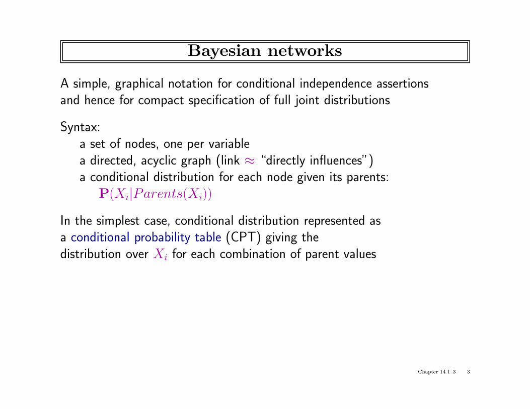
A simple, graphical notation for conditional independence assertionsand hence for compact specification of full joint distributions

Syntax:a set of nodes, one per variablea directed, acyclic graph (link ≈ “directly influences”)a conditional distribution for each node given its parents:

P(Xi|Parents(Xi))

In the simplest case, conditional distribution represented asa conditional probability table (CPT) giving thedistribution over Xi for each combination of parent values

Chapter 14.1–3 3

Example

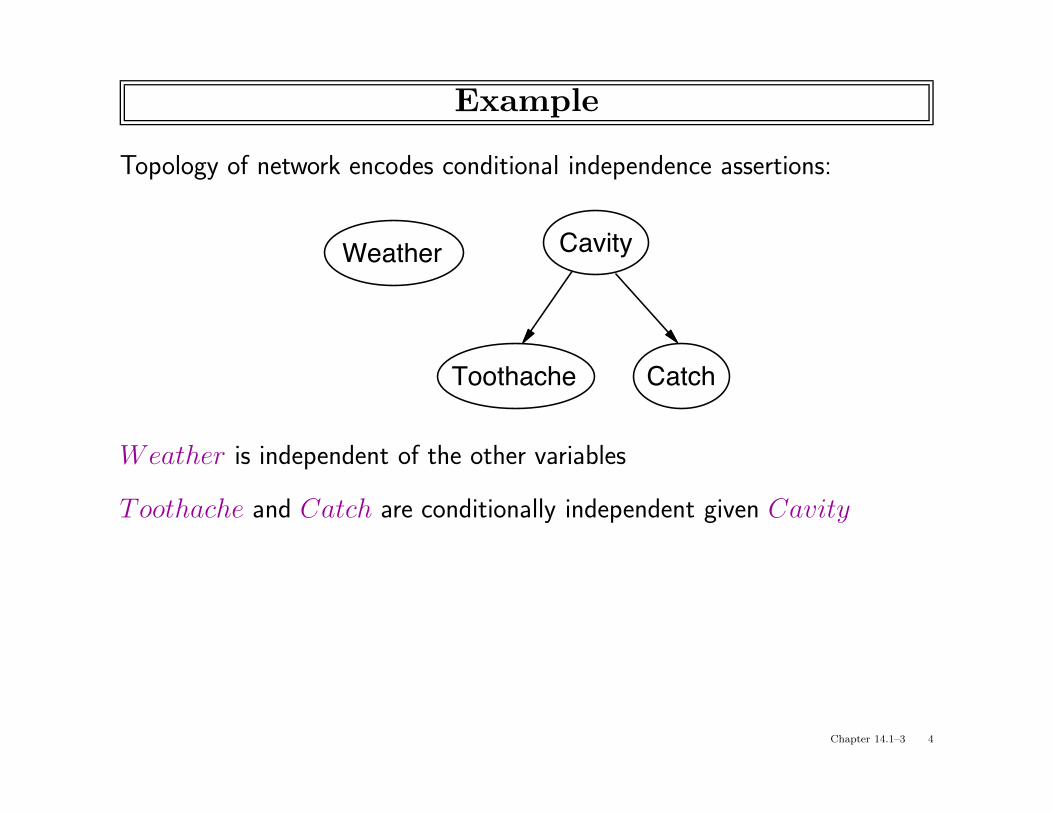
Topology of network encodes conditional independence assertions:

Weather Cavity

Toothache Catch

Weather is independent of the other variables

Toothache and Catch are conditionally independent given Cavity

Chapter 14.1–3 4

Example

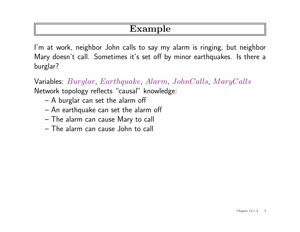
I’m at work, neighbor John calls to say my alarm is ringing, but neighborMary doesn’t call. Sometimes it’s set off by minor earthquakes. Is there aburglar?

Variables: Burglar, Earthquake, Alarm, JohnCalls, MaryCallsNetwork topology reflects “causal” knowledge:

– A burglar can set the alarm off– An earthquake can set the alarm off– The alarm can cause Mary to call– The alarm can cause John to call

Chapter 14.1–3 5

Example contd.

.001P(B)

.002P(E)

Alarm

Earthquake

MaryCallsJohnCalls

Burglary

BTTFF

ETFTF

.95

.29

.001

.94

P(A|B,E)

ATF

.90

.05

P(J|A) ATF

.70

.01

P(M|A)

Chapter 14.1–3 6

Compactness

A CPT for Boolean Xi with k Boolean parents hasB E

J

A

M

2k rows for the combinations of parent values

Each row requires one number p for Xi = true(the number for Xi = false is just 1 − p)

If each variable has no more than k parents,the complete network requires O(n · 2k) numbers

I.e., grows linearly with n, vs. O(2n) for the full joint distribution

For burglary net, 1 + 1 + 4 + 2 + 2 = 10 numbers (vs. 25 − 1 = 31)

Chapter 14.1–3 7

Global semantics

Global semantics defines the full joint distributionB E

J

A

M

as the product of the local conditional distributions:

P (x1, . . . , xn) = Πni = 1P (xi|parents(Xi))

e.g., P (j ∧ m ∧ a ∧ ¬b ∧ ¬e)

=

Chapter 14.1–3 8

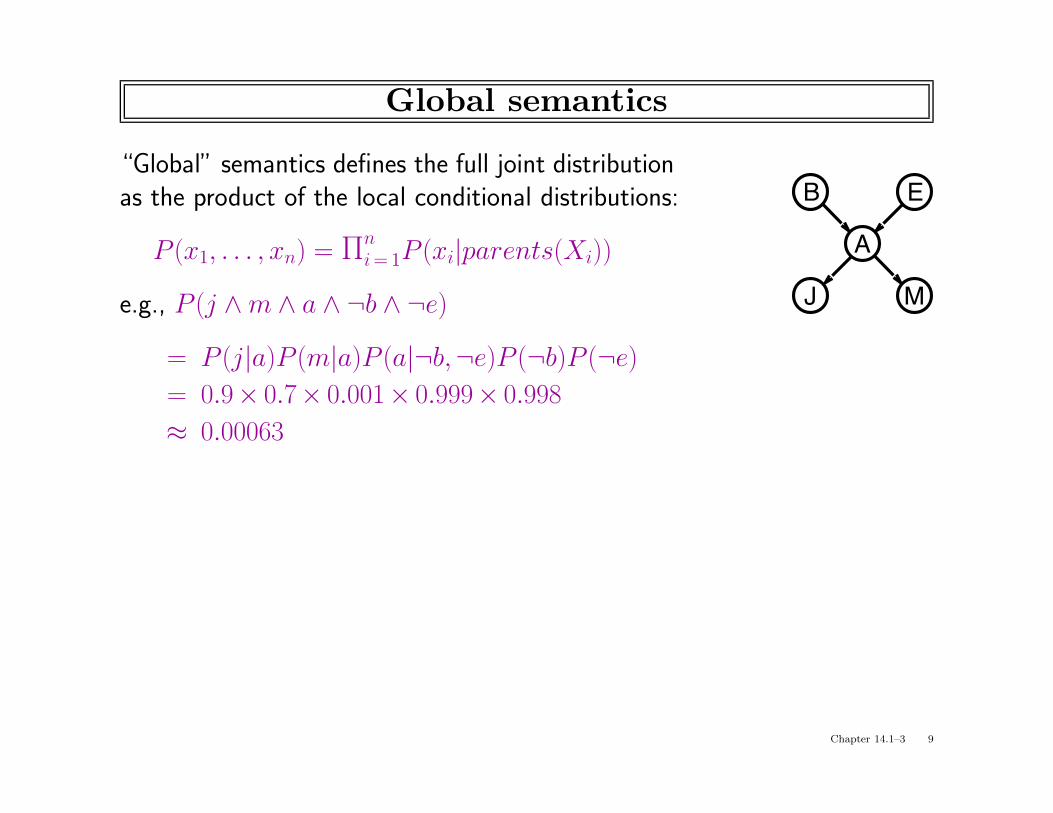
Global semantics

“Global” semantics defines the full joint distributionB E

J

A

M

as the product of the local conditional distributions:

P (x1, . . . , xn) = Πni = 1P (xi|parents(Xi))

e.g., P (j ∧ m ∧ a ∧ ¬b ∧ ¬e)

= P (j|a)P (m|a)P (a|¬b,¬e)P (¬b)P (¬e)

= 0.9× 0.7× 0.001× 0.999× 0.998

≈ 0.00063

Chapter 14.1–3 9

Local semantics

Local semantics: each node is conditionally independentof its nondescendants given its parents

. . .

. . .U1

X

Um

Yn

Znj

Y1

Z1j

Theorem: Local semantics ⇔ global semantics

Chapter 14.1–3 10

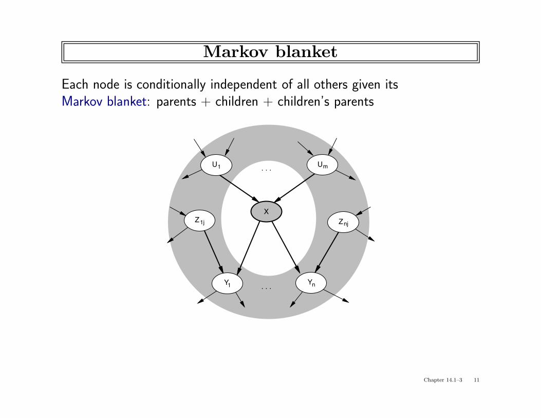
Markov blanket

Each node is conditionally independent of all others given itsMarkov blanket: parents + children + children’s parents

. . .

. . .U1

X

Um

Yn

Znj

Y1

Z1j

Chapter 14.1–3 11

Constructing Bayesian networks

Need a method such that a series of locally testable assertions ofconditional independence guarantees the required global semantics

1. Choose an ordering of variables X1, . . . , Xn

2. For i = 1 to nadd Xi to the networkselect parents from X1, . . . ,Xi−1 such that

P(Xi|Parents(Xi)) = P(Xi|X1, . . . , Xi−1)

This choice of parents guarantees the global semantics:

P(X1, . . . ,Xn) = Πni = 1P(Xi|X1, . . . , Xi−1) (chain rule)

= Πni = 1P(Xi|Parents(Xi)) (by construction)

Chapter 14.1–3 12

Inference tasks

Simple queries: compute posterior marginal P(Xi|E= e)e.g., P (NoGas|Gauge = empty, Lights = on, Starts= false)

Conjunctive queries: P(Xi,Xj|E= e) = P(Xi|E= e)P(Xj|Xi,E= e)

Optimal decisions: decision networks include utility information;probabilistic inference required for P (outcome|action, evidence)

Value of information: which evidence to seek next?

Sensitivity analysis: which probability values are most critical?

Explanation: why do I need a new starter motor?

Chapter 14.4–5 3

Inference by enumeration

Slightly intelligent way to sum out variables from the joint without actuallyconstructing its explicit representation

Simple query on the burglary network:B E

J

A

M

P(B|j, m)= P(B, j, m)/P (j, m)= αP(B, j,m)= α Σe Σa P(B, e, a, j, m)

Rewrite full joint entries using product of CPT entries:P(B|j, m)= α Σe Σa P(B)P (e)P(a|B, e)P (j|a)P (m|a)= αP(B) Σe P (e) Σa P(a|B, e)P (j|a)P (m|a)

Recursive depth-first enumeration: O(n) space, O(dn) time

Chapter 14.4–5 4

Enumeration algorithm

function Enumeration-Ask(X,e, bn) returns a distribution over Xinputs: X, the query variable

e, observed values for variables Ebn, a Bayesian network with variables {X} ∪ E ∪ Y

Q(X )← a distribution over X, initially emptyfor each value xi of X do

extend e with value xi for XQ(xi)←Enumerate-All(Vars[bn],e)

return Normalize(Q(X ))

function Enumerate-All(vars,e) returns a real numberif Empty?(vars) then return 1.0Y←First(vars)if Y has value y in e

then return P (y | Pa(Y )) × Enumerate-All(Rest(vars),e)else return

∑y P (y | Pa(Y )) × Enumerate-All(Rest(vars),ey)

where ey is e extended with Y = y

Chapter 14.4–5 5

Evaluation tree

P(j|a).90

P(m|a).70 .01

P(m| a)

.05P(j| a) P(j|a)

.90

P(m|a).70 .01

P(m| a)

.05P(j| a)

P(b).001

P(e).002

P( e).998

P(a|b,e).95 .06

P( a|b, e).05P( a|b,e)

.94P(a|b, e)

Enumeration is inefficient: repeated computatione.g., computes P (j|a)P (m|a) for each value of e

Chapter 14.4–5 6

Inference by variable elimination

Variable elimination: carry out summations right-to-left,storing intermediate results (factors) to avoid recomputation

P(B|j, m)= αP(B)

︸ ︷︷ ︸B

Σe P (e)︸ ︷︷ ︸

E

Σa P(a|B, e)︸ ︷︷ ︸

A

P (j|a)︸ ︷︷ ︸

J

P (m|a)︸ ︷︷ ︸

M= αP(B)ΣeP (e)ΣaP(a|B, e)P (j|a)fM(a)= αP(B)ΣeP (e)ΣaP(a|B, e)fJ(a)fM(a)= αP(B)ΣeP (e)ΣafA(a, b, e)fJ(a)fM(a)= αP(B)ΣeP (e)fAJM(b, e) (sum out A)= αP(B)fEAJM(b) (sum out E)= αfB(b)× fEAJM(b)

Chapter 14.4–5 7

Variable elimination: Basic operations

Summing out a variable from a product of factors:move any constant factors outside the summationadd up submatrices in pointwise product of remaining factors

Σxf1 × · · · × fk = f1 × · · · × fi Σx fi+1 × · · · × fk = f1 × · · · × fi × fX

assuming f1, . . . , fi do not depend on X

Pointwise product of factors f1 and f2:f1(x1, . . . , xj, y1, . . . , yk)× f2(y1, . . . , yk, z1, . . . , zl)

= f(x1, . . . , xj, y1, . . . , yk, z1, . . . , zl)E.g., f1(a, b)× f2(b, c) = f(a, b, c)

Chapter 14.4–5 8

Pointwise Product

Pointwise multiplication of factors when variable is summed out or atlast step

Pointwise product of factors f1 and f2:f1(x1, . . . , xj, y1, . . . , yk)× f2(y1, . . . , yk, z1, . . . , zl) = f(x1, . . . , xj, y1, . . . , yk, z1, . . . , zl)

E.g. f1(a, b)× f2(b, c) = f(a, b, c) :

a b f1(a, b) b c f2(b, c) a b c f(a, b, c)

T T .3 T T .2 T T T .3 * .2T F .7 T F .8 T T F .3 * .8F T .9 F T .6 T F T .7 * .6F F .1 F F .4 T F F .7 * .4

F T T .9 * .2F T F .9 * .8F F T .1 * .6F F F .1 * .4

F. C. Langbein, Artificial Intelligence – IV. Uncertain Knowledge and Reasoning; 4. Inference in Bayesian Networks 7

Summing Out

Summing out a variable from a product of factorsMove any constant factors outside the summationAdd up sub-matrices in pointwise product of remaining factors

�

x

f1 × · · ·× fk = f1 × · · ·× fl ×

�

x

fl+1 × · · ·× fk

= f1 × · · ·× fl × fX

E.g.�

af(a, b, c) = fa(b, c) :

a b c f(a, b, c) b c fa(b, c)

T T T .3 * .2 T T .3 * .2 + .9 * .2T T F .3 * .8 T F .3 * .8 + .9 * .8T F T .7 * .6 F T .7 * .6 + .1 * .6T F F .7 * .4 F F .7 * .4 + .1 * .4F T T .9 * .2F T F .9 * .8F F T .1 * .6F F F .1 * .4

F. C. Langbein, Artificial Intelligence – IV. Uncertain Knowledge and Reasoning; 4. Inference in Bayesian Networks 8

Variable elimination algorithm

function Elimination-Ask(X,e, bn) returns a distribution over Xinputs: X, the query variable

e, evidence specified as an eventbn, a belief network specifying joint distribution P(X1, . . . , Xn)

factors← [ ]; vars←Reverse(Vars[bn])for each var in vars do

factors← [Make-Factor(var ,e)|factors]if var is a hidden variable then factors←Sum-Out(var, factors)

return Normalize(Pointwise-Product(factors))

Chapter 14.4–5 9

Irrelevant variables

Consider the query P (JohnCalls|Burglary = true)B E

J

A

M

P (J |b) = αP (b)∑

eP (e)

∑

aP (a|b, e)P (J |a)

∑

mP (m|a)

Sum over m is identically 1; M is irrelevant to the query

Thm 1: Y is irrelevant unless Y ∈Ancestors({X}∪E)

Here, X = JohnCalls, E= {Burglary}, andAncestors({X}∪E) = {Alarm,Earthquake}so MaryCalls is irrelevant

(Compare this to backward chaining from the query in Horn clause KBs)

Chapter 14.4–5 10

Complexity of exact inference

Singly connected networks (or polytrees):– any two nodes are connected by at most one (undirected) path– time and space cost of variable elimination are O(dkn)

Multiply connected networks:– can reduce 3SAT to exact inference ⇒ NP-hard– equivalent to counting 3SAT models ⇒ #P-complete

A B C D

1 2 3

AND

0.5 0.50.50.5

LL

L

L1. A v B v C

2. C v D v A

3. B v C v D

Chapter 14.4–5 12