B. Rosner, W. Wang and E. Hibert Channing Division of Network Medicine

Harvard Medical School

Motivating example

1. The Nurses’ Health Study started in 1976 when 121,700 female nurses age 30-55 completed a medical questionnaire by mail

2. Dietary data was collected from the NHS subjects in 1980, 1984, 1986, 1990 and every 4 years afterward

3. 1989/1990 32,826 participants in the Nurses’ Health Study provided a blood sample

2

Motivating example (cont.)

4. Plasma carotenoid values were analyzed and used in a nested case-control study of breast cancer

5. Plasma carotenoid values from controls were related to dietary intake from 1990 food frequency questionnaire dietary intake in the NHS

6. Two approaches for calculating dietary carotenoid scores were considered.

3

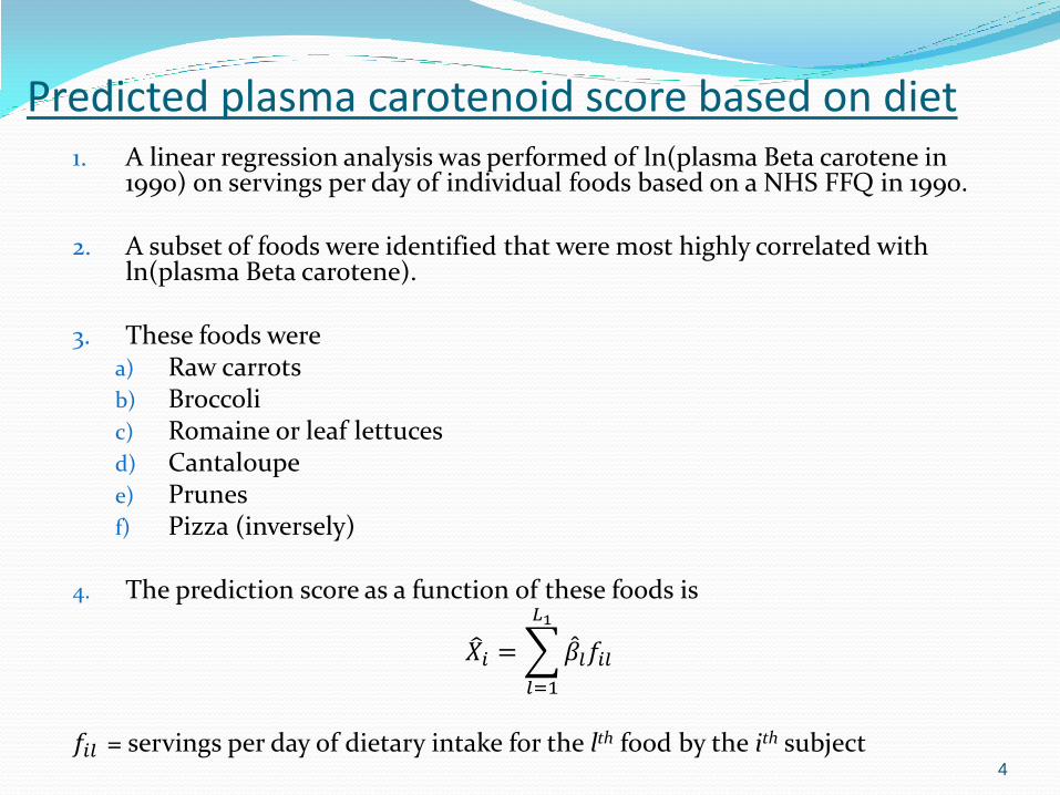
Predicted plasma carotenoid score based on diet 1. A linear regression analysis was performed of ln(plasma Beta carotene in

1990) on servings per day of individual foods based on a NHS FFQ in 1990.

2. A subset of foods were identified that were most highly correlated with ln(plasma Beta carotene).

3. These foods were a) Raw carrots b) Broccoli c) Romaine or leaf lettuces d) Cantaloupe e) Prunes f) Pizza (inversely)

4. The prediction score as a function of these foods is

𝑋 𝑖 = 𝛽 𝑙𝑓𝑖𝑙

𝐿1

𝑙=1

𝑓𝑖𝑙 = servings per day of dietary intake for the lth food by the ith subject

4

Observed dietary carotenoid score

5

1. We used published values of carotenoid contents for individual foods to obtain an observed dietary Beta carotene score given by

𝑌 𝑖 = 𝑤𝑙𝑓𝑖𝑙

𝐿2

𝑙=1

where 𝑤𝑙 = published Beta carotene content of the lth food 2. An assumption of the observed dietary Beta carotene

score is that Beta carotene from all foods is equally bioavailable

Comparison of dietary Beta carotene scores

6

Let Zi = observed ln(plasma Beta carotene) for the ith subject. Question: Is Xi or Yi more highly correlated with Zi?

7

Example – Nurses’ Health Study

Main study data N = 100 X = ln(predicted plasma Beta carotene 1990) Y = ln(dietary Beta carotene 1990) Z = ln(plasma Beta carotene 1990)

8

Reproducibility data

1. Predicted and dietary Beta carotene in 1984 and 1986, N = 40,266.

2. We assumed that true dietary Beta carotene would not change over a 2-year period.

9

Descriptive statistics for Predicted (X), Dietary (Y) and Plasma Beta carotene (Z), Nurses’ Health Study, 1990.

Pearson

(Spearman)

correlation

ICC**

variable GM* X Y Z

X (predicted) 237† 1.0 0.73

(0.78)

0.46

(0.40)

0.59

(0.61)

Y (dietary)

3400‡ 1.0 0.30

(0.27)

0.61

(0.60)

Z (plasma)

249† 1.0 -----

*Geometric mean

**Intraclass correlation between 1984 and 1986 dietary Beta carotene

†μg/L

‡ IU

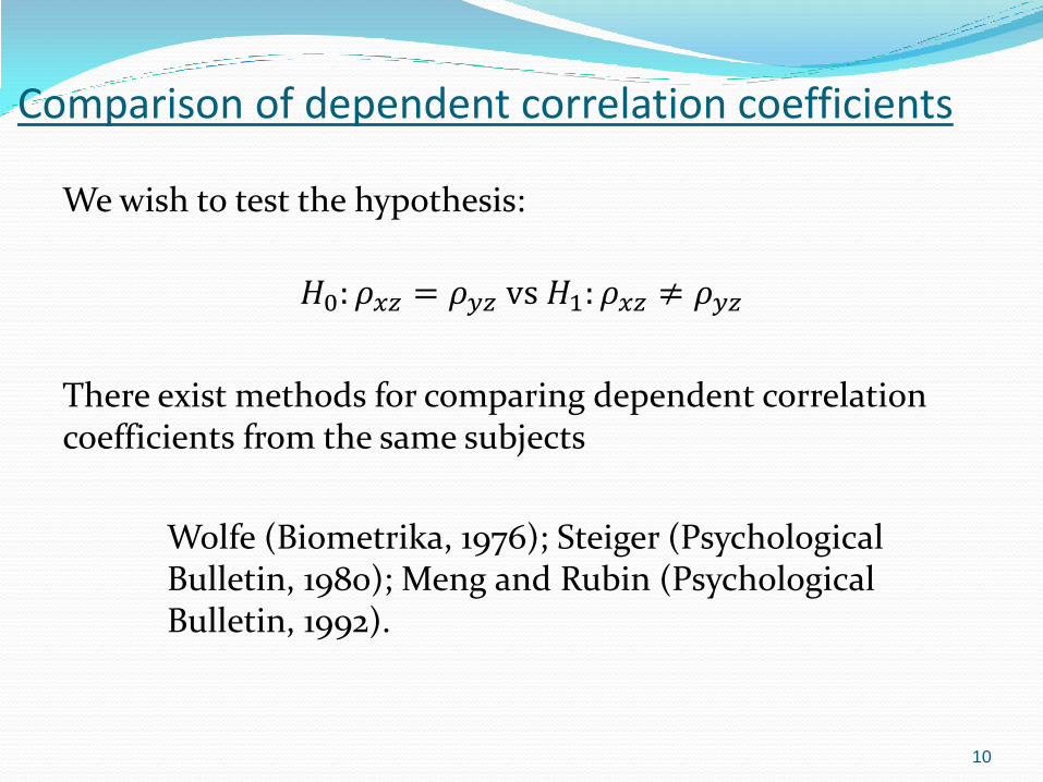
Comparison of dependent correlation coefficients

We wish to test the hypothesis:

𝐻0: 𝜌𝑥𝑧 = 𝜌𝑦𝑧 vs 𝐻1: 𝜌𝑥𝑧 ≠ 𝜌𝑦𝑧

There exist methods for comparing dependent correlation coefficients from the same subjects

Wolfe (Biometrika, 1976); Steiger (Psychological Bulletin, 1980); Meng and Rubin (Psychological Bulletin, 1992).

10

Comparison of Dependent Correlation Coefficients (Williams JRSS, 1959)

For example in a review paper by Steiger(1980) the approach of Williams(1959) (which is an enhancement of an earlier method by Hotelling) is recommended based on the test statistic on the next slide, since it preserves type I error under a variety of parameter values.

11

Comparison of Dependent Correlation Coefficients (Williams JRSS, 1959)(cont.)

12

1 3 0

2 3

.

2 2 2

.

( 1)(1 )( ) ~ u n d e r H ,

2 ( 1)(1 )

3

w h e re

1 R R

R 1 R 1 2 ,

R R 1

a n d

R ( ) / 2 .

x y

x z y z N

Z x y

x y x z

x y y z x z y z x y x z y z x y

x z y z

Z x z y z

N RT R R t

NR R R

N

R R R R R R R

R R

Classical Measurement Error model (1)

𝑋𝑖𝑗 = 𝛼𝑥 + 𝜇𝑥𝑖 + 𝑒𝑥𝑖𝑗, 𝑖 = 1, … , 𝑁1, 𝑗 = 1, … , 𝑘

𝑌𝑖𝑗= 𝛼𝑦 + 𝜇𝑦𝑖 + 𝑒𝑦𝑖𝑗, 𝑖 = 1, … , 𝑁1, 𝑗 = 1, … , 𝑘

where

(a) 𝜇𝑥𝑖 and 𝑒𝑥𝑖𝑗 are independent of each other

(b) 𝜇𝑦𝑖 and 𝑒𝑦𝑖𝑗 are independent of each other

(c) 𝜇𝑥𝑖 , 𝜇𝑦𝑖 are correlated

(d) 𝑒𝑥𝑖𝑗, 𝑒𝑦𝑖𝑗

are correlated if replicate measures of X and Y are

obtained from the same subjects

13

(1)

Classical Measurement Error model (2)

𝜇𝑥𝑖 and 𝜇𝑦𝑖 represent average values of X and Y over a large

number of replicates

(e.g., average FFQ scores over many replicates not that far apart in time.)

14

Comparison of dependent correlation coefficients (cont.)

Issue: Both Xi and Yi are measured with error

Related question: Are the true values of Xi and Yi denoted by μxi

and μyi equally correlated with Zi?

𝐻0: 𝑐𝑜𝑟𝑟 𝜇𝑥𝑖, 𝑍𝑖 = 𝑐𝑜𝑟𝑟 𝜇𝑦𝑖

, 𝑍𝑖 vs. 𝐻1 : 𝑐𝑜𝑟𝑟 𝜇𝑥𝑖, 𝑍𝑖 ≠ 𝑐𝑜𝑟𝑟 𝜇𝑦𝑖

, 𝑍𝑖

15

Deattenuated correlation between (Xi, Zi), (Yi, Zi)

1. We define the true (deattenuated) correlation between (X and Z) and (Y and Z) by

𝜌𝑥𝑧,𝑡𝑟𝑢𝑒 = 𝑐𝑜𝑟𝑟(𝜇𝑋𝑖, 𝑍𝑖)

𝜌𝑦𝑧,𝑡𝑟𝑢𝑒 = 𝑐𝑜𝑟𝑟(𝜇𝑌𝑖, 𝑍𝑖)

2. It is straightforward to show that based on equation 1,

𝜌𝑥𝑧,𝑡𝑟𝑢𝑒 = 𝜌𝑥𝑧/ 𝐼𝐶𝐶𝑥

𝜌𝑦𝑧,𝑡𝑟𝑢𝑒 = 𝜌𝑦𝑧/ 𝐼𝐶𝐶𝑦

where 𝐼𝐶𝐶𝑥, 𝐼𝐶𝐶𝑦 are the intraclass correlations obtained from repeated measures of X and Y, respectively.

16

Deattenuated correlation between (Xi, Zi), (Yi, Zi) (cont.)

3. Thus, the deattenuated correlation coefficient depends on

a) observed correlation between X and Z

b) intraclass correlation among replicate measures

17

Comparison of deattenuated correlation coefficients

1. We wish to test the hypothesis 𝐻0: 𝜌𝑥𝑧,𝑡𝑟𝑢𝑒 = 𝜌𝑦𝑧,𝑡𝑟𝑢𝑒 vs 𝐻1: 𝜌𝑥𝑧,𝑡𝑟𝑢𝑒 ≠ 𝜌𝑦𝑧,𝑡𝑟𝑢𝑒

2. Note that it is possible that 𝜌𝑥𝑧 = 𝜌𝑦𝑧, while 𝜌𝑥𝑧,𝑡𝑟𝑢𝑒 > 𝜌𝑦𝑧,𝑡𝑟𝑢𝑒 if

the reproducibility of X is worse then that of Y (i.e., 𝐼𝐶𝐶𝑥 < 𝐼𝐶𝐶𝑦)

3. Similarly, it is also possible that 𝜌𝑥𝑧 < 𝜌𝑦𝑧, while 𝜌𝑥𝑧,𝑡𝑟𝑢𝑒 = 𝜌𝑦𝑧,𝑡𝑟𝑢𝑒

18

Hypothesis Testing

1. We will base inference on Fisher’s z-transform and will test the equivalent hypothesis:

𝐻0: 𝑍𝑥𝑧,𝑡𝑟𝑢𝑒 = 𝑍𝑦𝑧,𝑡𝑟𝑢𝑒 vs 𝐻1: 𝑍𝑥𝑧,𝑡𝑟𝑢𝑒 ≠ 𝑍𝑦𝑧,𝑡𝑟𝑢𝑒

where 𝑍𝑥𝑧,𝑡𝑟𝑢𝑒 = 0.5 ln 1 + 𝜌𝑥𝑧,𝑡𝑟𝑢𝑒 / 1 − 𝜌𝑥𝑧,𝑡𝑟𝑢𝑒

and

𝑍𝑦𝑧,𝑡𝑟𝑢𝑒 is defined similarly.

19

Hypothesis Testing (cont.)

2. We will use the test statistic 𝑉𝑥𝑦,𝑡𝑟𝑢𝑒 defined by:

𝑉 𝑥𝑦,𝑡𝑟𝑢𝑒 =𝑍 𝑥𝑧,𝑡𝑟𝑢𝑒 − 𝑍 𝑦𝑧,𝑡𝑟𝑢𝑒

𝑣𝑎𝑟(𝑍 𝑥𝑧,𝑡𝑟𝑢𝑒 − 𝑍 𝑦𝑧,𝑡𝑟𝑢𝑒)

where 𝑣𝑎𝑟 𝑍 𝑥𝑧,𝑡𝑟𝑢𝑒 − 𝑍 𝑦𝑧,𝑡𝑟𝑢𝑒

= 𝑣𝑎𝑟 𝑍 𝑥𝑧,𝑡𝑟𝑢𝑒 + 𝑣𝑎𝑟 𝑍 𝑦𝑧,𝑡𝑟𝑢𝑒

− 2𝑐𝑜𝑣 (𝑍 𝑥𝑧,𝑡𝑟𝑢𝑒, 𝑍 𝑦𝑧,𝑡𝑟𝑢𝑒)

20

(2)

Hypothesis Testing (cont.)

3. We assume asymptotic normality of 𝑉 𝑥𝑦,𝑡𝑟𝑢𝑒 with large sample 2-sided p-value given by

p-value = 2 x 1 − Φ |𝑉 𝑥𝑦,𝑡𝑟𝑢𝑒|

where Φ(x) = standard normal cdf

4. Asymptotic normality will hold if

a) n = number of subjects in the main study (used to estimate the interclass correlations) ∞

b) n1 = number of subjects in the reproducibility study ∞

c) k = number of replicates per subject (≥2) is fixed

21

22

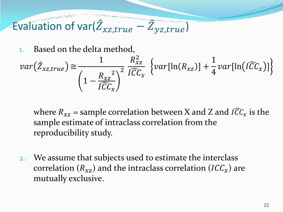
Evaluation of var(𝑍 𝑥𝑧,𝑡𝑟𝑢𝑒 − 𝑍 𝑦𝑧,𝑡𝑟𝑢𝑒)

1. Based on the delta method,

𝑣𝑎𝑟 𝑍 𝑥𝑧,𝑡𝑟𝑢𝑒 ≅1

1 −𝑅𝑥𝑧

2

𝐼𝐶𝐶 𝑥

2 𝑅𝑥𝑧

2

𝐼𝐶𝐶 𝑥

𝑣𝑎𝑟[ln 𝑅𝑥𝑧 ] +1

4𝑣𝑎𝑟[ln 𝐼𝐶𝐶

𝑥 ]

where 𝑅𝑥𝑧 = sample correlation between X and Z and 𝐼𝐶𝐶 𝑥 is the

sample estimate of intraclass correlation from the reproducibility study.

2. We assume that subjects used to estimate the interclass correlation (𝑅𝑥𝑧) and the intraclass correlation (𝐼𝐶𝐶𝑥) are mutually exclusive.

23

Evaluation of var(𝑍 𝑥𝑧,𝑡𝑟𝑢𝑒 − 𝑍 𝑦𝑧,𝑡𝑟𝑢𝑒) (cont.)

3. Closed form expressions based on the delta method exist for

𝑣𝑎𝑟 𝑙𝑛 𝑅𝑥𝑧 based on the method of moments and the delta method.

4. For 𝑣𝑎𝑟[ln 𝐼𝐶𝐶 𝑥 ] we use the delta method and the work of

Donner (International Statistical Review 1986; 54: 67-82) to obtain

𝑣𝑎𝑟 ln 𝐼𝐶𝐶 𝑥 ≅

2 1 − 𝐼𝐶𝐶 𝑥

2[1 + 𝑘1 − 1 𝐼𝐶𝐶

𝑥]

𝐼𝐶𝐶 𝑥2𝑘1(𝑘1 − 1)(𝑛1 − 1)

where 𝑛1 = number of subjects in the reproducibility study for x

𝑘1 = number of replicates per subject in the reproducibility study for x

24

Evaluation of var(𝑍 𝑥𝑧,𝑡𝑟𝑢𝑒 − 𝑍 𝑦𝑧,𝑡𝑟𝑢𝑒) (cont.)

5. Similarly based on the delta method, closed form expressions

exist for 𝑣𝑎𝑟 𝑍 𝑦𝑧,𝑡𝑟𝑢𝑒 and 𝑐𝑜𝑣 𝑍 𝑥𝑧,𝑡𝑟𝑢𝑒 , 𝑍 𝑦𝑧,𝑡𝑟𝑢𝑒

6. Thus, we can evaluate the test statistic 𝑉 𝑥𝑦,𝑡𝑟𝑢𝑒 in equation 2

and perform the hypothesis test

Interval Estimation for 𝜌𝑥𝑧,𝑡𝑟𝑢𝑒 − 𝜌𝑦𝑧,𝑡𝑟𝑢𝑒

1. It is also of interest to obtain confidence limits for ∆𝜌,𝑡𝑟𝑢𝑒= 𝜌𝑥𝑧,𝑡𝑟𝑢𝑒 −

𝜌𝑦𝑧,𝑡𝑟𝑢𝑒

2. Large sample two-sided 100% x (1-α) confidence limits for ∆𝜌,𝑡𝑟𝑢𝑒 are given by

∆ 𝑅,𝑡𝑟𝑢𝑒 ± 𝑧1−𝛼/2 𝑣𝑎𝑟(∆ 𝑅,𝑡𝑟𝑢𝑒)

where

∆ 𝑅,𝑡𝑟𝑢𝑒= 𝑅𝑥𝑧,𝑡𝑟𝑢𝑒 − 𝑅𝑦𝑧,𝑡𝑟𝑢𝑒

𝑣𝑎𝑟 ∆ 𝑅,𝑡𝑟𝑢𝑒

= 𝑅𝑥𝑧,𝑡𝑟𝑢𝑒2 𝑣𝑎𝑟[ln(𝑅𝑥𝑧,𝑡𝑟𝑢𝑒)] + 𝑅𝑦𝑧,𝑡𝑟𝑢𝑒

2 𝑣𝑎𝑟[ln ( 𝑅𝑦𝑧,𝑡𝑟𝑢𝑒)]

− 2𝑅𝑥𝑧,𝑡𝑟𝑢𝑒𝑅𝑦𝑧,𝑡𝑟𝑢𝑒 𝑐𝑜𝑣[ln(𝑅𝑥𝑧,𝑡𝑟𝑢𝑒), ln(𝑅𝑦𝑧,𝑡𝑟𝑢𝑒)]

The delta method and method of moments estimators are used to obtain closed form

expressions for the components of 𝑣𝑎𝑟 ∆ 𝑅,𝑡𝑟𝑢𝑒

25

(3)

Comparison of dependent correlation coefficients (without correction for deattenuation)

1. Similar methods can be used to test the hypothesis

𝐻0: 𝜌𝑥𝑧 = 𝜌𝑦𝑧 𝑣𝑠 𝐻1: 𝜌𝑥𝑧 ≠ 𝜌𝑦𝑧

based on the large sample test statistic

𝑉 𝑥𝑦 =𝑍 𝑥𝑧−𝑍 𝑦𝑧

𝑣𝑎𝑟(𝑍 𝑥𝑧−𝑍 𝑦𝑧) ~ 𝑁 0,1 for large N

with two-sided p-value = 2 x 1 − Φ |𝑉 𝑥𝑦| .

26

(4)

Comparison of dependent Spearman correlations

1. We can also consider the comparison of dependent Spearman correlations (𝜌𝑥𝑧,𝑠, 𝜌𝑦𝑧,𝑠) where we test the

hypothesis 𝐻0: 𝜌𝑥𝑧,𝑠 = 𝜌𝑦𝑧,𝑠𝑣𝑠 𝐻1: 𝜌𝑥𝑧,𝑠 ≠ 𝜌𝑦𝑧,𝑠

2. To our knowledge, this has not been considered before

3. This is more appropriate for skewed data where there is no obvious transformation to normality as is true in both of our examples.

27

Assessment of Variability for Ranked Data (1)

1. ANOVA-type methods are used to express between and within-subject variability for normally distributed data (as in the previous slides)

2. However, these methods are not appropriate for rank scales.

3. We need a measure analogous to μx for ranked scales for the purpose of studying between and within-subject variability for ranked data.

28

Assessment of Variability for Ranked Data (2)

1. Suppose we have data Zi, Xi1, …, Xik for the ith subject, i=1, …, n1; j=1, …, k in the reproducibility study , where

Zi = plasma value for the ith subject

Xij = score for the jth replicate of the ith subject

2. Let Pi,z = c.d.f. of Zi within the reference population

Pij,x* = c.d.f. of Xij within the reference population at the jth time point

3. Thus, Pr(Z≤Zi)= Pi,z and

Pr(Xj≤Xij)= Pij,x*

Pearson (1907) referred to Pi,z and Pij,x* as grades for the ith subject for Z

and Xj, respectively.

29

Assessment of Variability for Ranked Data (3)

4. If Ri,z = rank of Zi among the n1 Z values and

Rij,x* = rank of Xij among the n1 X.j values

then 𝑃 𝑖,𝑧 = 𝑅𝑖𝑧/(𝑛1 + 1) and 𝑃𝑖𝑗,𝑥∗ = 𝑅𝑖𝑗,𝑥

∗ /(𝑛1 + 1) are sample estimates

of the grades 𝑃𝑖,𝑧 and 𝑃𝑖𝑗,𝑥∗

30

Assessment of Variability for Ranked Data (4)

1. We need a model to express variability of 𝑃𝑖𝑗∗ over

repeated replicates j on a scale where variability is independent of the level of 𝑃𝑖𝑗

∗ .

2. For this purpose, we define the underlying probit of the grades by

𝐻𝑖,𝑧 = Φ−1 𝑃𝑖,𝑧 , 𝐻𝑖𝑗,𝑥∗ = Φ−1(𝑃𝑖𝑗,𝑥

∗ )

where Φ−1 = inverse normal c.d.f.

3. By definition, the probits will be normally distributed and the variability of the probits will be constant across levels of 𝐻𝑖,𝑧 and 𝐻𝑖𝑗,𝑥

∗ .

31

Assessment of Variability for Ranked Data (5)

4. Hence, we consider a random effects ANOVA model on the probit scale given by

𝐻𝑖𝑗,𝑥

∗ = 𝛼𝑖,𝑥 + 𝑒𝑖𝑗,𝑥 , 𝑖 = 1, … , 𝑛1, 𝑗 = 1, … , 𝑘

where 𝛼𝑖,𝑥~𝑁 0, 𝜎𝐴,𝑥2 , 𝑒𝑖𝑗,𝑥~𝑁(0, 𝜎𝑥

2)

and 𝑒𝑖𝑗,𝑥 is independent of 𝛼𝑖,𝑥

5. Note that based on equation 5 we assume that the variability of 𝐻𝑖𝑗,𝑥

∗ is independent of the average level, an assumption which

is more reasonable on the probit scale than the original c.d.f. scale.

32

(5)

Deattenuation for probit scores

1. Since the probit scores are normally distributed we can use similar ANOVA-type methods to estimate the deattenuated correlation between the probit score for Z and the probit score for X given by

𝜌𝑥𝑧,𝑝𝑟𝑜𝑏𝑖𝑡,𝑡𝑟𝑢𝑒 = 𝜌𝑥𝑧,𝑝𝑟𝑜𝑏𝑖𝑡 / 𝐼𝐶𝐶𝑥,𝑝𝑟𝑜𝑏𝑖𝑡

where

𝜌𝑥𝑧,𝑝𝑟𝑜𝑏𝑖𝑡 is obtained from the main study used to estimate interclass correlation between sample probits of X and Z.

𝐼𝐶𝐶𝑥,𝑝𝑟𝑜𝑏𝑖𝑡 is obtained from a random effects ANOVA fitted from replicate probit scores in the reproducibility study.

33

Deattenuation for rank scores (estimated grades)

1. Our goal is to define a correlation similar to 𝜌𝑥𝑧,𝑝𝑟𝑜𝑏𝑖𝑡,𝑡𝑟𝑢𝑒 on the grade (rank) scale.

2. Note that grades on the probit scale and grades on the original scale are the same because the probit is a rank-preserving transformation.

3. We define the grade of Zi for the ith subject by Φ(𝐻𝑖,𝑧) and the underlying grade of the dietary (FFQ) score for the ith subject by

Φ(𝛼𝑖,𝑥).

4. Thus,

𝜌𝑥𝑧,𝑠,𝑡𝑟𝑢𝑒 = 𝑐𝑜𝑟𝑟(Ρ𝑖,𝑧 , Ρ𝑖,𝑥∗ ) = 𝑐𝑜𝑟𝑟[Φ(𝐻𝑖,𝑧), Φ(𝛼𝑖,𝑥)]

while

𝜌𝑥𝑧,𝑝𝑟𝑜𝑏𝑖𝑡,𝑡𝑟𝑢𝑒 = corr(𝐻𝑖,𝑧, 𝛼𝑖,𝑥)

34

Relationship between Deattenuated correlations on the probit and grade scales

1. However, because 𝐻𝑖,𝑧 and 𝛼𝑖,𝑥 are normally distributed scales there is an exact relationship between rank correlation and Pearson correlation (Moran, Biometrika, 1948) given by

Deattenuated rank correlation = 𝜌𝑥𝑧,𝑠,𝑡𝑟𝑢𝑒 = (6 𝜋 )𝑠𝑖𝑛−1(𝜌𝑥𝑧,𝑝𝑟𝑜𝑏𝑖𝑡,𝑡𝑟𝑢𝑒 2 )

35

(6)

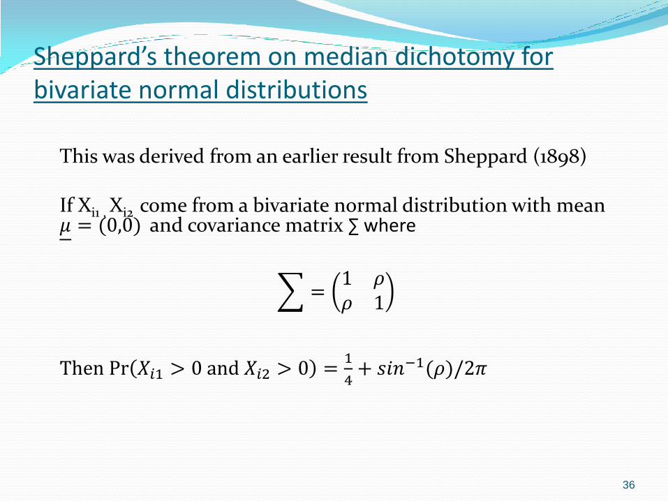
Sheppard’s theorem on median dichotomy for bivariate normal distributions

This was derived from an earlier result from Sheppard (1898) If Xi1 , Xi2 come from a bivariate normal distribution with mean 𝜇 = (0,0) and covariance matrix ∑ where

=1 𝜌𝜌 1

Then Pr 𝑋𝑖1 > 0 and 𝑋𝑖2 > 0 =1

4+ 𝑠𝑖𝑛−1(𝜌)/2𝜋

36

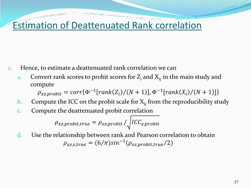
Estimation of Deattenuated Rank correlation

2. Hence, to estimate a deattenuated rank correlation we can

a. Convert rank scores to probit scores for Zi and Xij in the main study and compute

𝜌𝑥𝑧,𝑝𝑟𝑜𝑏𝑖𝑡 = 𝑐𝑜𝑟𝑟 Φ−1 𝑟𝑎𝑛𝑘 𝑍𝑖 𝑁 + 1 , Φ−1[𝑟𝑎𝑛𝑘 𝑋𝑖 𝑁 + 1 ]

b. Compute the ICC on the probit scale for Xij from the reproducibility study

c. Compute the deattenuated probit correlation

𝜌𝑥𝑧,𝑝𝑟𝑜𝑏𝑖𝑡,𝑡𝑟𝑢𝑒 = 𝜌𝑥𝑧,𝑝𝑟𝑜𝑏𝑖𝑡 / 𝐼𝐶𝐶𝑥,𝑝𝑟𝑜𝑏𝑖𝑡

d. Use the relationship between rank and Pearson correlation to obtain 𝜌𝑥𝑧,𝑠,𝑡𝑟𝑢𝑒 = (6 𝜋 )𝑠𝑖𝑛−1(𝜌𝑥𝑧,𝑝𝑟𝑜𝑏𝑖𝑡,𝑡𝑟𝑢𝑒 2 )

37

Estimation of grade correlation

1. In a previous paper (Rosner and Glynn, Statistics in Medicine, 2007) we defined an alternative estimator for the grade correlation

𝜌 𝑠,𝑎 = (6 𝜋 )𝑠𝑖𝑛−1(𝑅𝑝𝑟𝑜𝑏𝑖𝑡 2 )

and compared it to the ordinary Spearman rank correlation coefficient

𝜌 𝑠 = 𝑅𝑠

2. In simulation studies we showed that the relative efficiency of 𝜌 𝑠,𝑎 to

𝜌 𝑠 = MSE (𝜌 𝑠,𝑎)/MSE(𝜌 𝑠) ranged from 0.83-0.92 in samples of size 100 and that there was a similar slight negative bias for both estimators.

3. We also showed that the asymptotic relative efficiency (ARE) of 𝜌 𝑠,𝑎 vs. 𝜌 𝑠 = 9/𝜋2 ≈ 0.91 when 𝜌 𝑠 = 0.

38

Comparison of dependent deattenuated Spearman correlations (Hypothesis Testing)

1. We have previously (Rosner and Glynn, Statistics in Medicine, 2007) defined the deattenuated Spearman correlation by

𝜌𝑥𝑧,𝑠,𝑡𝑟𝑢𝑒 = 6 𝜋 sin−1 𝜌𝑥𝑧,𝑝𝑟𝑜𝑏𝑖𝑡,𝑡𝑟𝑢𝑒/2

2. Hence, the hypothesis 𝐻0: 𝜌𝑥𝑧,𝑠,𝑡𝑟𝑢𝑒 = 𝜌𝑦𝑧,𝑠,𝑡𝑟𝑢𝑒 𝑣𝑠 𝐻1: 𝜌𝑥𝑧,𝑠,𝑡𝑟𝑢𝑒 ≠ 𝜌𝑦𝑧,𝑠,𝑡𝑟𝑢𝑒 is equivalent to the hypothesis

𝐻0: 𝜌𝑥𝑧,𝑝𝑟𝑜𝑏𝑖𝑡,𝑡𝑟𝑢𝑒 = 𝜌𝑦𝑧,𝑝𝑟𝑜𝑏𝑖𝑡,𝑡𝑟𝑢𝑒 vs 𝐻1: 𝜌𝑥𝑧,𝑝𝑟𝑜𝑏𝑖𝑡,𝑡𝑟𝑢𝑒 ≠ 𝜌𝑦𝑧,𝑝𝑟𝑜𝑏𝑖𝑡,𝑡𝑟𝑢𝑒

which can be tested using the methods in equation 2.

3. Similarly, we can obtain interval estimates for

∆𝑠,𝑡𝑟𝑢𝑒= 𝜌𝑥𝑧,𝑠,𝑡𝑟𝑢𝑒 − 𝜌𝑦𝑧,𝑠,𝑡𝑟𝑢𝑒

using similar methods as in equation 3.

39

Comparison of dependent Spearman correlations

1. We can also consider the comparison of dependent Spearman correlations to test the hypothesis

𝐻0: 𝜌𝑥𝑧,𝑠 = 𝜌𝑦𝑧,𝑠 𝑣𝑠 𝐻1: 𝜌𝑥𝑧,𝑠 ≠ 𝜌𝑦𝑧,𝑠

2. Based on previous slides, if the data are transformed to the probit scale, then from Rosner and Glynn (Statistics in Medicine, 2007)

𝜌𝑥𝑧,𝑠 =6

𝜋sin−1 𝜌𝑥𝑧,𝑝𝑟𝑜𝑏𝑖𝑡/2

3. Thus, the hypothesis test in (7) is equivalent to 𝐻0: 𝜌𝑥𝑧,𝑝𝑟𝑜𝑏𝑖𝑡 = 𝜌𝑦𝑧,𝑝𝑟𝑜𝑏𝑖𝑡 𝑣𝑠 𝐻1: 𝜌𝑥𝑧,𝑝𝑟𝑜𝑏𝑖𝑡 ≠ 𝜌𝑦𝑧,𝑝𝑟𝑜𝑏𝑖𝑡

and we can use the methods in equation 2 based on the probit scores to test this hypothesis.

40

(7)

Interval Estimation of 𝜌𝑥𝑧,𝑠 − 𝜌𝑦𝑧,𝑠

1. Our point estimate is 𝑅𝑥𝑧,𝑠 − 𝑅𝑦𝑧,𝑠 = ∆ 𝜌,𝑠

𝑅𝑥𝑧,𝑠 =6

𝜋sin−1 𝑅𝑥𝑧,𝑝𝑟𝑜𝑏𝑖𝑡/2

𝑅𝑦𝑧,𝑠 is defined similarly

2. A 100% x (1- 𝛼) CI for ∆𝜌,𝑠 is given by

∆𝑅,𝑠 ± 𝑍1−𝛼/2 𝑣𝑎𝑟(𝑅𝑥𝑧,𝑠 − 𝑅𝑦𝑧,𝑠 )

and

𝑣𝑎𝑟 𝑅𝑥𝑧,𝑠 − 𝑅𝑦𝑧,𝑠 = 𝑣𝑎𝑟 𝑅𝑥𝑧,𝑠 + 𝑣𝑎𝑟 𝑅𝑦𝑧,𝑠 − 2𝑐𝑜𝑣(𝑅𝑥𝑧,𝑠, 𝑅𝑦𝑧,𝑠 )

is estimated using the delta method.

41

42

Simulation study-design – main study

1. We simulated data for (X, Y, Z) ~ N (μ, Ʃ) with

𝜇 = 0,0,0 and =

1 0.732 𝜌𝑥𝑧

0.732 1 𝜌𝑦𝑧

𝜌𝑥𝑧 𝜌𝑦𝑧 1

which was approximately the correlation structure in our example

X = ln (predicted Beta carotene)

Y = ln (dietary Beta carotene)

Z = ln (plasma Beta carotene)

2. 4,000 simulations were performed for each combination of N = 100, 400 and 𝜌𝑥𝑧 = 𝜌𝑦𝑧 = 0.305, 0.50.

43

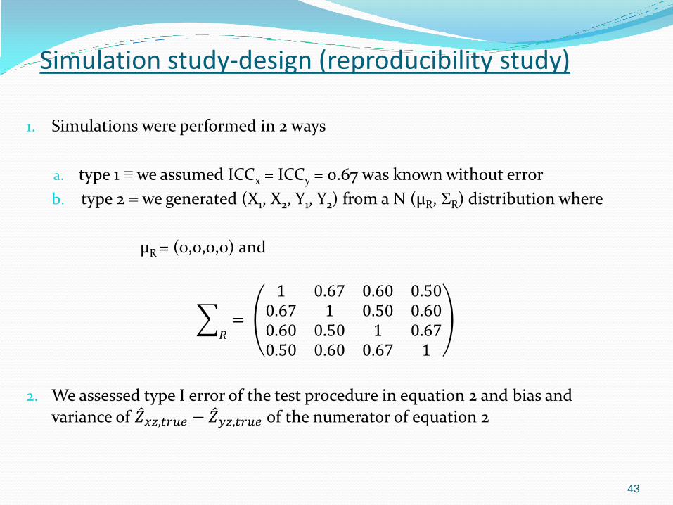
Simulation study-design (reproducibility study)

1. Simulations were performed in 2 ways

a. type 1 ≡ we assumed ICCx = ICCy = 0.67 was known without error

b. type 2 ≡ we generated (X1, X2, Y1, Y2) from a N (μR, ƩR) distribution where

μR = (0,0,0,0) and

=

1 0.67 0.60 0.500.67 1 0.50 0.600.60 0.50 1 0.670.50 0.60 0.67 1

𝑅

2. We assessed type I error of the test procedure in equation 2 and bias and

variance of 𝑍 𝑥𝑧,𝑡𝑟𝑢𝑒 − 𝑍 𝑦𝑧,𝑡𝑟𝑢𝑒 of the numerator of equation 2

44

Simulation study results, 𝜌𝑥𝑧 = 𝜌𝑦𝑧 = 0.305, ICCx = ICCy = 0.67,

4,000 simulations

(𝑍 𝑥𝑧,𝑡𝑟𝑢𝑒−𝑍 𝑦𝑧,𝑡𝑟𝑢𝑒) Type I error

Type ρxz (ρyz) N Mean Variance*

1 0.305 100 theoretical 0 95 0.050

empirical -0.002 103 0.061

400 theoretical 0 24 0.050

empirical -0.001 23 0.045

2 0.305 100 theoretical 0 100 0.050

empirical 0.003 106 0.050

400 theoretical 0 25 0.050

empirical 0.001 25 0.047

*x 10-4

45

1. The procedure has little bias and appropriate variance for both N = 100 and 400

2. Variance is slightly higher for type 2 simulations when the ICC is estimated rather than type 1 simulations when it is assumed known

3. Empirical Type I error ranges from 0.045 – 0.061 which is adequate

4. Similar results were obtained for the case 𝜌𝑥𝑧 = 𝜌𝑦𝑧= 0.50.

Simulation study results (cont.)

46

Simulation study – coverage probability for 𝜌𝑥𝑧,𝑡𝑟𝑢𝑒 − 𝜌𝑦𝑧,𝑡𝑟𝑢𝑒

We also considered coverage probability for ∆𝜌,𝑡𝑟𝑢𝑒

based on the procedure in equation 3 using the type 2 simulation design previously described.

47

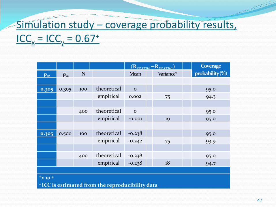
Simulation study – coverage probability results, ICCx = ICCy = 0.67+

(𝐑𝑥𝑧,𝑡𝑟𝑢𝑒−𝐑𝑦𝑧,𝑡𝑟𝑢𝑒) Coverage

probability (%) ρxz ρyz N Mean Variance*

0.305 0.305 100 theoretical 0 95.0

empirical 0.002 75 94.3

400 theoretical 0 95.0

empirical -0.001 19 95.0

0.305 0.500 100 theoretical -0.238 95.0

empirical -0.242 75 93.9

400 theoretical -0.238 95.0

empirical -0.238 18 94.7

*x 10-4 + ICC is estimated from the reproducibility data

48

Simulation study – coverage probability (cont.)

The bias in the estimation of 𝜌𝑥𝑧,𝑡𝑟𝑢𝑒 − 𝜌𝑦𝑧,𝑡𝑟𝑢𝑒 is small

and the coverage probability ranges from 93.9% – 95.0% which is adequate.

49

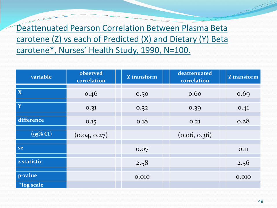
Deattenuated Pearson Correlation Between Plasma Beta carotene (Z) vs each of Predicted (X) and Dietary (Y) Beta carotene*, Nurses’ Health Study, 1990, N=100.

variable observed

correlation Z transform

deattenuated

correlation Z transform

X 0.46 0.50 0.60 0.69

Y 0.31 0.32 0.39 0.41

difference 0.15 0.18 0.21 0.28

(95% CI) (0.04, 0.27) (0.06, 0.36)

se 0.07 0.11

z statistic 2.58 2.56

p-value 0.010 0.010 *log scale

50

Nurses’ Health Study – Pearson correlations

1. There is a significant difference between a) Pearson correlation for plasma Beta carotene (Z)

vs log (predicted dietary Beta carotene) = X, R=0.46, and

b) The Pearson correlation for plasma Beta carotene (Z) vs log (dietary Beta carotene) = Y, R=0.31 (p-value = 0.010)

2. Both Rxz and Ryz become larger after correction for deattenuation (Rxz, true = 0.60; Ryz,true = 0.39) and remain significantly different (p-value = 0.010)

51

Deattenuated Spearman Correlation Between Plasma Beta carotene (Z) vs each of Predicted (X) and Dietary (Y) Beta carotene, Nurses’ Health Study, 1990, N=100.

variable

observed

Spearman

correlation

observed

probit

correlation

Z

transform

deattenuated

Spearman

correlation

deattenuated

probit

correlation

Z

transform

X 0.40 0.42 0.44 0.51 0.52 0.58

Y 0.27 0.28 0.29 0.35 0.36 0.38

difference 0.13 0.14 0.15 0.16 0.16 0.20

(95% CI) (0.02, 0.24) (0.02, 0.30)

se 0.07 0.09

z statistic 2.33 2.24

p-value 0.020 0.025

52

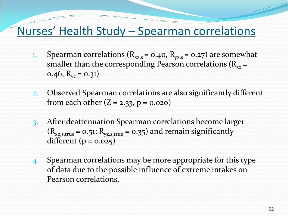
Nurses’ Health Study – Spearman correlations

1. Spearman correlations (Rxz,s = 0.40, Ryz,s = 0.27) are somewhat smaller than the corresponding Pearson correlations (Rxz = 0.46, Ryz = 0.31)

2. Observed Spearman correlations are also significantly different from each other (Z = 2.33, p = 0.020)

3. After deattenuation Spearman correlations become larger (Rxz,s,true = 0.51; Ryz,s,true = 0.35) and remain significantly different (p = 0.025)

4. Spearman correlations may be more appropriate for this type of data due to the possible influence of extreme intakes on Pearson correlations.

53

Comparison of storage conditions for HbA1c measurements in plasma

1. Epidemiologic studies have begun using dried blood spot assays of HgbA1c as a biomarker

2. A study was conducted at Brigham & Women’s Hospital (BWH) to test the hypothesis that dried blood determinations for HbA1c are valid in low-intensity storage conditions

3. Blood samples were drawn by standard phlebotomy into EDTA containing tubes and submitted for duplicate HPLC analysis of HbA1c to the BWH Hematology Laboratory.

54

Comparison of storage conditions for HbA1c measurements in plasma (cont.)

1. Samples were air dried for at least 20 minutes and then placed into single sample airtight bags

2. Samples were stored at room temperature for 1, 2 or 4 weeks and then shipped to Biosafe Laboratories for HbA1c analysis (conditions 1-3) or placed in freezer storage (-80°C) for an additional 4 or 12 weeks (conditions 4-6, 7-9)

3. Dried blood spot determination of HbA1c were performed in triplicate, blinded to storage conditions and protocol.

55

HbA1c processing-definition of gold standard and surrogate measures

1. For this example, we define Z = the gold standard = HbA1c determination with 0 weeks of room temperature storage pre-shipping and no freezer storage (i.e., immediate processing)

2. We define the surrogate measure X = HbA1c determination after 2 weeks of room temperature storage pre-shipping and an additional 4 weeks of freezer storage after shipping ≡ short-term storage

3. We define the surrogate measure Y = HbA1c determination after 4 weeks of room temperature storage pre-shipping and an additional 12 weeks of freezer storage after shipping ≡ long-term storage

56

HbA1c processing-correlation analysis

1. We wish to compare corr(X,Z) vs. corr(Y,Z)

2. There were only 12 subjects with X, Y and Z available for analysis

3. Furthermore, distributions of HbA1c were somewhat skewed

4. Hence, Spearman correlation coefficients rather than Pearson correlations were used

57

HbA1c processing – data analysis

1. We wish to test the hypothesis:

𝐻0: 𝜌𝑥𝑧,𝑠 = 𝜌𝑦𝑧,𝑠 vs. 𝐻1: 𝜌𝑥𝑧,𝑠 ≠ 𝜌𝑦𝑧,𝑠

2. Due to the small sample size, exact permutation-based

methods were used to estimate levels of significance

3. X, Y and Z samples were ranked and then converted to the probit scale using the transformation

𝐻𝑥 = Φ−1 𝑟𝑎𝑛𝑘 𝑋 𝑁 + 1 and similarly for Hy, Hz.

58

HbA1c processing – data analysis (cont.)

4. The test statistic

𝑉𝑥𝑦,𝑝𝑟𝑜𝑏𝑖𝑡 =𝑍 𝑥𝑧,𝑝𝑟𝑜𝑏𝑖𝑡 − 𝑍 𝑦𝑧,𝑝𝑟𝑜𝑏𝑖𝑡

𝑣𝑎𝑟(𝑍𝑥𝑧,𝑝𝑟𝑜𝑏𝑖𝑡 − 𝑍𝑦𝑧,𝑝𝑟𝑜𝑏𝑖𝑡)

was computed based on the observed data 5. The permutation distribution of 𝑉𝑥𝑦,𝑝𝑟𝑜𝑏𝑖𝑡 was obtained by randomly

shuffling X and Y labels and denoted by 𝑉𝑥𝑦,𝑝𝑟𝑜𝑏𝑖𝑡,𝑝𝑒𝑟𝑚

6. The exact p-value was estimated by

p − value = 2 x 𝐼 𝑉𝑥𝑦,𝑝𝑟𝑜𝑏𝑖𝑡,𝑝𝑒𝑟𝑚,𝑚 ≥ |𝑉𝑥𝑦,𝑝𝑟𝑜𝑏𝑖𝑡,𝑜𝑏𝑠𝑒𝑟𝑣𝑒𝑑| /𝑀

𝑀

𝑚=1

where m = 212 = 4096.

59

HbA1c processing – data analysis – correction for deattenuation

1. Dried blood spot determination of HbA1c were performed in triplicate, blinded to storage conditions and protocol

2. The triplicates were used to calculate the intraclass correlations (ICC), separately for each storage condition. The ICC was used to correct for deattenuation.

3. We wish to test the hypothesis

𝐻0: 𝜌𝑥𝑧,𝑠,𝑡𝑟𝑢𝑒 = 𝜌𝑦𝑧,𝑠,𝑡𝑟𝑢𝑒 vs. 𝐻1: 𝜌𝑥𝑧,𝑠,𝑡𝑟𝑢𝑒 ≠ 𝜌𝑦𝑧,𝑠,𝑡𝑟𝑢𝑒

which is equivalent to the hypothesis

𝐻0: 𝜌𝑥𝑧,𝑝𝑟𝑜𝑏𝑖𝑡,𝑡𝑟𝑢𝑒 = 𝜌𝑦𝑧,𝑝𝑟𝑜𝑏𝑖𝑡,𝑡𝑟𝑢𝑒 vs. 𝐻1: 𝜌𝑥𝑧,𝑝𝑟𝑜𝑏𝑖𝑡,𝑡𝑟𝑢𝑒 ≠ 𝜌𝑦𝑧,𝑝𝑟𝑜𝑏𝑖𝑡,𝑡𝑟𝑢𝑒

60

HbA1c processing – data analysis – correction for deattenuation (cont.)

4. We calculate the test statistic

𝑉𝑥𝑦,𝑝𝑟𝑜𝑏𝑖𝑡 =𝑍 𝑥𝑧,𝑝𝑟𝑜𝑏𝑖𝑡,𝑡𝑟𝑢𝑒 − 𝑍 𝑦𝑧,𝑝𝑟𝑜𝑏𝑖𝑡,𝑡𝑟𝑢𝑒

𝑣𝑎𝑟(𝑍 𝑥𝑧,𝑝𝑟𝑜𝑏𝑖𝑡,𝑡𝑟𝑢𝑒 − 𝑍 𝑦𝑧,𝑝𝑟𝑜𝑏𝑖𝑡,𝑡𝑟𝑢𝑒)

where

𝑍 𝑥𝑧,𝑝𝑟𝑜𝑏𝑖𝑡,𝑡𝑟𝑢𝑒 = 0.5𝑙𝑛1 + 𝑅𝑥𝑧,𝑝𝑟𝑜𝑏𝑖𝑡,𝑡𝑟𝑢𝑒

1 − 𝑅𝑥𝑧,𝑝𝑟𝑜𝑏𝑖𝑡,𝑡𝑟𝑢𝑒

and

𝑅𝑥𝑧,𝑝𝑟𝑜𝑏𝑖𝑡,𝑡𝑟𝑢𝑒 =𝑅𝑥𝑧,𝑝𝑟𝑜𝑏𝑖𝑡

𝐼𝐶𝐶𝑥,𝑝𝑟𝑜𝑏𝑖𝑡

and 𝑍 𝑦𝑧,𝑝𝑟𝑜𝑏𝑖𝑡,𝑡𝑟𝑢𝑒 is defined similarly.

5. We then permuted the X, Y labels and determined the permutation p-value

𝑝 − 𝑣𝑎𝑙𝑢𝑒𝑡𝑟𝑢𝑒 = 2 x 𝐼 𝑉𝑥𝑦,𝑝𝑟𝑜𝑏𝑖𝑡,𝑡𝑟𝑢𝑒,𝑝𝑒𝑟𝑚,𝑚 ≥ |𝑉𝑥𝑦,𝑝𝑟𝑜𝑏𝑖𝑡,𝑡𝑟𝑢𝑒,𝑜𝑏𝑠𝑒𝑟𝑣𝑒𝑑| /𝑀

𝑀

𝑚=1

HbA1c processing – data analysis

1. The permutation distribution of Vxy,probit is given on the next slide.

2. The distribution of Vxy,probit is symmetric about 0, but doesn’t look normal.

61

, ,3 . T h e d is tr ib u tio n o f V is a lso sym m e tr ic

a b o u t 0 , b u t h a s e v e n lo n g e r ta ils .

4 . T h e c o m p le te re su lts w ith a n d w ith o u t d e a tte n u a tio n

a re g iv e n tw o s lid e s a h e a d .

xy p ro b it tru e

62

63

Spearman Correlation Between HbA1c levels determined immediately vs. HbA1c levels determined after 2 delay periods

observed

Spearman

correlation

observed

probit

correlation

Z

transform

deattenuated

Spearman

correlation

deattenuated

probit

correlation

Z

transform ICC

Short-term

storage* 0.984 0.985 2.458 0.988 0.989 2.604 0.945

Long-term

storage** 0.743 0.759 0.994 0.787 0.801 1.102 0.895

v statistic 3.728 3.002

p-value (large

sample) 0.0002 0.0027

p-value

(exact) 0.010 0.010

*short-term = 2 weeks of room temperature storage pre-shipping + additional 4 weeks of freezer storage after shipping

**long-term = 4 weeks of room temperature storage pre-shipping + additional 12 weeks of freezer storage after shipping

64

Spearman Correlation analysis – HbA1c data - discussion

1. There were significant differences between the validity of the short-term and long-term HbA1c determination both with and without correction for deattenuation with HbA1c from short-term storage more highly correlated with HbA1c after immediate processing than HbA1c from long-term storage.

2. Exact p-values are more appropriate in this setting and are considerably larger than large sample p-values

3. Correction for deattenuation is modest because ICC’s were relatively high in this example

65

Summary

1. We have presented a method for comparing deattenuated correlation coefficents (𝜌𝑥𝑧,𝑡𝑟𝑢𝑒 , 𝜌𝑦𝑧,𝑡𝑟𝑢𝑒)

estimated from the same subjects.

2. This method can compare the validity of two surrogate measures (X, Y) where validity is measured by the respective correlations with a third variable (Z) and both X and Y are measured with error.

3. Confidence limits for both 𝜌𝑥𝑧,𝑡𝑟𝑢𝑒 − 𝜌𝑦𝑧,𝑡𝑟𝑢𝑒 and

𝜌𝑥𝑧 − 𝜌𝑦𝑧 are also provided.

66

Summary (cont.)

4. An assumption is that (X, Y, Z) are multivariate normal.

5. The methods are asymptotic, but we have shown that finite sample properties are adequate for N ≥ 100.

6. We also consider permutation test methods to perform hypothesis testing in a small-sample setting.

67

Summary (cont.)

7. The methods were extended to the comparison of deattenuated Spearman correlations in the case where multivariate normality of (X, Y, Z) is not appropriate.

8. SAS macros to implement these methods are available from the authors upon request.