A Simple Model for Axial Displacement in a Cylindrical Pipe with Internal

Shock Loading

Neal P. Bitter and Joseph E. Shepherd

Graduate Aerospace Laboratories

California Institute of Technology

Pasadena, California 91125

Email: nbitter@caltech.edu

ABSTRACT

This paper describes a simplified model for predicting the axial displacement, stress, and strain in

pipes subjected to internal shock waves. This model involves the neglect of radial and rotary inertia of

the pipe, so its predictions represent the spatially-averaged or low-pass filtered response of the tube. The

simplified model is developed first by application of the physical principles of conservation of mass and

momentum on each side of the shock wave. This model is then reproduced using the mathematical theory

of the Green’s function, which allows other load and boundary conditions to be more easily incorporated.

Comparisons with finite element simulations demonstrate that the simple model adequately captures the

tube’s axial motion except near the critical velocity corresponding to the bar wave speed√

E/ρ. Near

this point the simplified model, despite being an unsteady model, predicts a time-independent resonance

while the finite element model predicts resonance that grows with time.

1

Introduction

Extensive experimental observations of the structural response of pipes and tubes to internal shock and deto-

nation wave loading have been carried out over the last decade at the Explosion Dynamics Laboratory, as docu-

mented in [1,2]. These observations consist primarily of point measurements of strain which have been extremely

useful for quantitative characterization of structural loading as well as point validation of simulations. However,

due to the large number of potential vibration modes and the stiffness of typical piping systems, it is often diffi-

cult to infer the global response due to the confounding presence of high-frequency oscillations in strain signals.

Finite-element simulations and reduced order models are particularly useful tools to use in conjunction with ex-

periments to gain insight into large-scale, lower frequency, response modes. This note presents an analysis of the

axial displacement induced by shock loading and proposes a simplified but quantitatively predictive model.

Numerical Simulation Results

One example for which we have carried out an analysis is a finite-element simulation (LS-Dyna) of a shock

wave with a pressure rise of 2.52 MPa traveling at 2088 m/s in 2-m long section of 2-in diameter schedule 40

stainless steel pipe (see Table 1). This example is relevant to the evaluation of the structural response of piping in

the Hydrogen in Pipes and Ancillary Vessels (HPAV) evaluation carried out for the Waste Treatment Plant at the

Hanford Site [3, 4].

Typical results are shown in Figs. 1 and 2 for at a time of 225 µs, before any wave reflections occur from

the RHS end of the pipe. The shock wave propagates with constant speed, starting from the origin at the LHS

and propagating toward the right. The fluid dynamics associated with the shock wave are not considered as we

are only interested in the structural response of the pipe to an idealized traveling load. The boundary conditions

are zero axial and radial displacement at each end of the pipe. The pipe is modeled as a linear elastic solid with

Young’s modulus E = 1.93×1011 Pa, density ρ = 8040 kg/m3, and Poisson’s ratio ν = 0.30. The inner radius of the

pipe is 26.25 mm and the wall thickness is 3.91 mm. For the membrane model of motion discussed subsequently,

the effective membrane radius a = 28.2 mm and the ratio a/h = 7.2.

The radial displacement w and axial displacement u propagate as progressive wave systems as shown in Fig. 3.

2

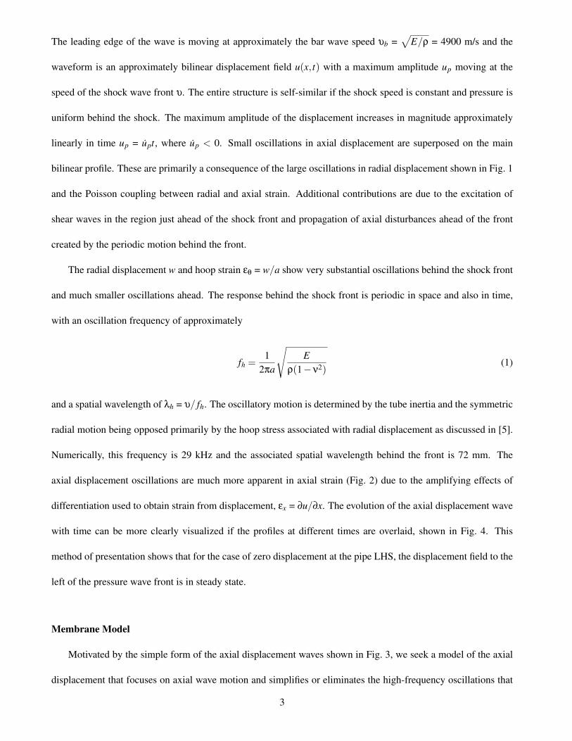
The leading edge of the wave is moving at approximately the bar wave speed υb =√

E/ρ = 4900 m/s and the

waveform is an approximately bilinear displacement field u(x, t) with a maximum amplitude up moving at the

speed of the shock wave front υ. The entire structure is self-similar if the shock speed is constant and pressure is

uniform behind the shock. The maximum amplitude of the displacement increases in magnitude approximately

linearly in time up = upt, where up < 0. Small oscillations in axial displacement are superposed on the main

bilinear profile. These are primarily a consequence of the large oscillations in radial displacement shown in Fig. 1

and the Poisson coupling between radial and axial strain. Additional contributions are due to the excitation of

shear waves in the region just ahead of the shock front and propagation of axial disturbances ahead of the front

created by the periodic motion behind the front.

The radial displacement w and hoop strain εθ = w/a show very substantial oscillations behind the shock front

and much smaller oscillations ahead. The response behind the shock front is periodic in space and also in time,

with an oscillation frequency of approximately

fh =1

2πa

√E

ρ(1−ν2)(1)

and a spatial wavelength of λh = υ/ fh. The oscillatory motion is determined by the tube inertia and the symmetric

radial motion being opposed primarily by the hoop stress associated with radial displacement as discussed in [5].

Numerically, this frequency is 29 kHz and the associated spatial wavelength behind the front is 72 mm. The

axial displacement oscillations are much more apparent in axial strain (Fig. 2) due to the amplifying effects of

differentiation used to obtain strain from displacement, εx = ∂u/∂x. The evolution of the axial displacement wave

with time can be more clearly visualized if the profiles at different times are overlaid, shown in Fig. 4. This

method of presentation shows that for the case of zero displacement at the pipe LHS, the displacement field to the

left of the pressure wave front is in steady state.

Membrane Model

Motivated by the simple form of the axial displacement waves shown in Fig. 3, we seek a model of the axial

displacement that focuses on axial wave motion and simplifies or eliminates the high-frequency oscillations that

3

are prominent in the axial strain results. The first step is to approximate the pipe as a shell without any shear

deformation or rotary inertia. This will eliminate the high frequency oscillations observed in the axial strain

just ahead of the pressure front in Fig. 2. The second step is to consider the shell as a membrane without any

bending stiffness or radial inertia to eliminate radial displacement oscillations, i.e., the radial motion is quasi-

steady in character. This will eliminate the hoop mode oscillations observed in the radial displacement but will

create discontinuities in radial displacement at the shock front as well as at the shell endpoints. Including bending

stiffness would smear these discontinuities over the characteristic bending length of the shell so this needs to be

kept in mind when interpreting the model results.

In adopting a quasi-steady membrane model of radial motion, we are effectively time-averaging the radial

displacement oscillations behind the front, replacing these by a mean response. This is a reasonable approximation

as long as the time scales of the radial oscillation are much smaller than the axial wave propagation times. In the

example discussed above, the period of radial oscillation is 34 µs and the time for pressure wave to travel the

length of the pipe (2 m) is 958 µs. So approximately 28 hoop oscillation cycles will occur in the time it take the

pressure wave to traverse the length of the pipe.

The axial motion of the tube is modeled using the following axial force balance:

ρh∂2u∂t2 =

∂Nx

∂x(2)

where Nx is the axial stress resultant, defined as the integral of axial stress through the wall thickness. Since we

are neglecting the radial dynamics and axial bending of the pipe and balancing the hoop stress against the pressure

load, the Lame solution [6] for a thick-walled pressure vessel can be used to model the variation of hoop and

radial stresses through the wall thickness. This model is valid only in regions of the pipe where the axial strain

is uniform in both the axial and radial directions, but due to our neglect of axial bending and rotary inertia these

conditions are met everywhere except near the load front and the boundaries of the pipe. As a result, the use of

the Lame solution is consistent with the assumptions already made in developing this simplified model. Note that

for thin tubes, one can alternatively use the thin shell approximations σr << σθ and σθ = Pa/h, but in the present

formulation the thick-wall effects can be included without additional difficulty.

4

The Lame solutions for the hoop and radial stresses in a long cylinder are the following:

σθ(r) =PR2

i

R2i −R2

o

(1+

R2o

r2

)(3a)

σr(r) =PR2

i

R2i −R2

o

(1− R2

o

r2

)(3b)

where Ri and Ro are the inner and outer radii of the tube. From Hooke’s law, the axial stress is then:

σx = Eεx +ν(σr +σθ)

= Eεx +ν2PR2

i

R2o−R2

i(4)

The axial stress resultant Nx is found by integrating σx through the wall thickness. Since in this case σx is uniform

through the thickness, the result is:

Nx = Ehεx +ν2PhR2

i

R2o−R2

i(5)

It may be noted that the wall thickness is h = Ro−Ri and the mean radius is a = 0.5(Ro +Ri). Using these

definitions, the axial stress resultant can be expressed in the form:

Nx = Ehεx +νPa(

R2i

a2

)(6)

The quantity in parenthesis is the correction due to thick-wall effects, which will hereafter be denoted Ct . As the

wall thickness is reduced, this factor approaches 1.0 and the expression that remains is the result from classical

thin shell theory. In this paper, the correction term must be retained since we are analyzing a tube with inner

radius Ri = 26.25 mm and mean radius a = 28.2 mm, which gives a correction factor of Ct = 0.866.

Upon inserting (6) into (2) and replacing εx = ∂u/∂x we obtain:

1υ2

b

∂2u∂t2 −

∂2u∂x2 =Ct

νaEh

∂P∂x

(7)

where υb is the bar wave speed√

E/ρ. This result is a wave equation for the axial displacement u which is forced

by the gradient of pressure. For a thin tube, the correction factor Ct tends to 1.0 and the quantity νPa/Eh is the

5

quasi-static radial displacement of the tube from classical thin shell theory. Thus the forcing term can also be

interpreted as the gradient of the quasi-static radial displacement.

In the context of traveling shock waves, the pressure distribution is modeled as:

P(x, t) = PoΘ(υt− x) (8)

where Θ is the Heaviside step function and υ is the speed of the shock wave. Under this load, (7) becomes:

1υ2

b

∂2u∂t2 −

∂2u∂x2 =Ct

νPoaEh

δ(υt− x) (9)

where δ(x) is the Dirac delta function. In this case, the source term vanishes everywhere except at the shock front

x = υt and the axial wave motion of the tube is driven solely by the discontinuity in pressure (which results in a

jump in hoop, axial, and radial stresses) at the wavefront.

Observations on the Numerical Simulation Results

The numerical solution exhibits a linear growth in time for both the spatial extent and amplitude of the axial

displacement u. The point of maximum displacement amplitude up moves with the speed of the pressure wave

and as shown in Fig. 5, and grows linearly with time with a speed of up = -0.035 m/s.

The axial displacement also shows a nearly linear variation with distance (Fig. 4) in the segments of the

wave ahead and behind the pressure wave front. We will therefore idealize the strain in these segments as time-

independent with distinct values ahead εx,1 and behind εx,2 of the wave front. From the continuity of the axial

displacement at the pressure wave front, we can integrate the strain through the wave to relate the two strain

magnitudes to the wave speeds and obtain the following relationship:

εx,1 =−υ

υb−υεx,2 (10)

6

In terms of up, the idealized strains can computed to be

εx,1 =−up

υb−υ(11)

and

εx,2 =up

υ(12)

Solution of the Model Equations

Based on the results of the numerical simulations, we can divide the solution domain into three segments:

Region 0: υbt ≤ x ≤ L. Ahead of bar wave front there is no disturbance and the axial displacement vanishes.

Once the wave reaches the RHS of the pipe, x = L, a reflected wave propagating the left is created in order to

satisfy the boundary condition. This wave can be readily computed using the method of characteristics [7] but in

the interest of brevity, will not be considered in this note. With this limitation, the solution is simply

u(x, t) = 0 for υbt ≤ x≤ L (13)

Region 1: υt ≤ x≤ υbt Between the pressure wave front and the bar wave front, the axial displacement propagates

as a right facing wave with constant axial strain εx,1 and stress resultant Nx,1. The magnitude of the strain was

given above by (11). Since the pressure is zero in this region, the axial stress resultant (6) reduces to

Nx = Ehεx (14)

which is consistent with the state of uni-axial strain ahead of the pressure wave front. From the theory of charac-

teristics for wave equations [7], the axial displacement in this region has the general form

u = f (x−υbt) (15)

7

From the assumption of constant axial strain in this region we conclude that

u(x, t) = εx,1 (x−υbt) (16)

which consistent with our previous observations. This implies that

∂u∂t

=−εx,1υb (17)

∂u∂x

= εx,1 (18)

Using (11), we can write the displacement field as

u(x, t) =−up

υb−υ(x−υbt) for υt ≤ x≤ υbt (19)

Region 2: 0 ≤ x ≤ υt - Between the LHS (x = 0) of the pipe and the pressure wave front x = υt, the displacement

is steady (independent of time) and linearly proportional to the distance from the LHS of the pipe.

∂u∂t

= 0 (20)

∂u∂x

= εx,2 (21)

This can be integrated to yield the complete solution

u(x, t) = εx,2x (22)

The axial stress resultant in this region is

Nx,2 = Ehεx,2 +νaPCt (23)

8

Using (12), we can write the displacement field as

u(x, t) =up

υx for 0≤ x≤ υt (24)

In order to complete the solution, we need one more relationship to determine the value of the strain in either

region 1 or 2 or else the magnitude of up. An additional relationship can be obtained by considering the axial

force balance in the shell on each side of the pressure front. In general, the axial stress resultants on each side will

be different in order to have a balance of momentum at the front that correctly accounts for the jump in material

velocity V = ∂u/∂t through the front.

The simplest way to construct the balance of momentum is to consider a fixed control volume that encloses

the shell. At time t the left boundary of the control volume is in region 2 just behind the pressure front, and the

right boundary is well in front of the bar wave, completely enclosing region 1. Recognizing that the velocity in

region 2 is zero, the change in momentum in a time ∆t will be the sum of the loss of momentum in the shell

material that is brought to rest by the motion of the front and the gain of momentum due to the motion of the bar

wave. This has to be balanced by the impulse applied to the control volume by the stress resultant in region 2,

since the stress resultant ahead of region 1 vanishes. The resulting momentum balance is

−Nx,2∆t = ρh(υb−υ)V1∆t (25)

Substituting for the axial stress resultant and the velocity, we have

Ehεx,2 +νaPCt =−ρh(υb−υ)(−εx,1υb) (26)

Substitutions of expressions for axial strains (11) and (12) leads to

up =−νυυb

υb +υ

ah

PE

Ct (27)

εx,2 =−νυb

υb +υ

ah

PE

Ct (28)

εx,1 =+νυυb

υ2b−υ2

ah

PE

Ct (29)

9

From Hooke’s law, the hoop strain is given by:

εθ =1E[σθ−ν(σx +σr)] (30)

At the outer surface of the tube, σr is zero and in region 2, σθ and σx are evaluated using (3a) and (4). Using these

equations, the hoop strain at the outer surface in region 2 is found to be:

εθ,2 =

(1−ν

2 υ

υb +υ

)PaEh

Ct (31)

In region 1, both σr and σθ are zero, so the application of (30) gives:

εθ,1 =−ν2 υυb

υ2b−υ2

PaEh

Ct (32)

As expected, εθ,2 is intermediate between the limiting cases of zero axial strain, εx,2 = 0, and zero axial stress, Nx,2

= 0, which give the limits

(1−ν

2) PaEh

Ct ≤ εθ,2 ≤PaEh

Ct (33)

Substituting the parameters listed in Table 1, we obtain the numerical values given in Table 2. The corre-

sponding LS-Dyna simulation results were analyzed to extract mean values for comparison to the model. Given

the simplifications of the model, the results compare favorably with the values computed by the transient finite-

element solution.

Green’s Function Solution

The exact solution for the axial displacements can also be found using the mathematical technique of the

Green’s function. To do so, (7) will be solved on a semi-infinite interval [0,∞] with the boundary condition

u(0, t) = 0 at the origin. The Green’s function g(x,xo, t, to) is found by replacing the inhomogeneous term in (7)

by spatial and temporal Dirac delta functions:

1υ2

b

∂2g∂t2 −

∂2g∂x2 = δ(x− xo)δ(t− to) (34)

10

The Green’s function satisfying this equation is given by [8]:

g(x,xo, t, to) =υb

2Θ

(υb(t− to)−|x− xo|

)

=

υb2 |x− xo|< υb(t− to)

0 |x− xo|> υb(t− to)(35)

where Θ is the Heaviside function. Solutions to the inhomogeneous wave equation (7) are found by integrating

the Green’s function against the source term:

u(x, t) =∫ t

0

∫∞

−∞

g(x,xo, t, to)CtνaEh

∂

∂xoP(xo, to)dxodto (36)

We are only interested in solutions on the interval [0,∞], but in order to evaluate this integral it is necessary to

specify the pressure P(xo, to) for xo < 0. To satisfy the boundary condition u(0, t) = 0, the pressure distribution is

mirrored symmetrically about the origin, i.e.,

P(−xo, to) = P(xo, to) (37)

Since the Green’s function is only non-zero when |x− xo|< υb(t− to), the limits of the spatial integral in (36) are

replaced by finite values and the solution can be written as

u(x, t) =Ctυb

2νaEh

∫ t

0

∫ x+υb(t−to)

x−υb(t−to)

∂

∂xoP(xo, to)dxodto (38)

which is readily integrated to obtain:

u(x, t) =Ctυb

2νaEh

∫ t

0P(

x+υb(t− to), to

)

−P(

x−υb(t− to), to

)dto (39)

The above result is valid for an arbitrary pressure distribution. We now specialize to the case of a shock wave

traveling at velocity υ, for which the pressure is a step function of amplitude Po:

P(xo, to) = PoΘ(υto− xo) (40)

11

Equation (39) can be interpreted as the integral of the applied pressure P along the C+ and C− characteristics,

where integration along these paths is parameterized by to. This situation is shown schematically on an x-t diagram

in Fig. 6. The right half of the diagram depicts the domain of interest, while the left half is the mirror image used

to satisfy the zero displacement boundary condition. There are two waves in the region of interest. The faster

wave, traveling at a speed υb, is the leading characteristic and in front of this wave (Region 0) no motion of the

tube occurs. The slower wave, traveling at speed υ, is the applied pressure load. Within the shaded region on this

plot, the applied pressure is constant and equal to Po, while outside this region the pressure is zero.

In this diagram we are seeking the solution u at a pair of coordinates (x, t). As represented in (39), the solution

at this point is found by integrating the pressure along the C+ and C− characteristics, shown as dashed lines in the

figure. If the point of interest lies in Region 2, as depicted by point (xa, ta), then both the C+ and C− characteristics

pass through the shaded region where the pressure is nonzero. On the other hand, for a point such as (xb, tb) lying

in Region 1, only the C+ characteristic passes through the shaded region. As a result, the form of the solution is

different in each of these regions.

Region 2

To evaluate (39) in Region 2, we need only to integrate from t1 < to < t along the C+ characteristic and from

t2 < to < t along the C− characteristic, where t1 and t2 are the times at which the characteristics intersect the

pressure wavefront. Thus (39) becomes:

u(x, t) =Ctυb

2νaEh

[∫ t

t1Podto−

∫ t

t2Podto

]

=Ctυb

2νaEh

Po(t1− t2) (41)

From the geometry of the problem, the times t1 and t2 are found to be:

t1 =υbt− xυ+υb

(42a)

t2 =x+υbtυ+υb

(42b)

12

Thus the displacement in region 2 is given by:

u(x, t) =−CtνaEh

Po

(υb

υ+υb

)x (x < υt) (43)

Region 1

The solution in Region 1 is found using the same approach; however, only the C+ characteristic passes through

the shaded region in Fig. 6. As a result, (39) becomes:

u(x, t) =Ctυb

2νaEh

Po(t4− t3) (44)

Referring to Fig. 6, t3 is exactly the same as t1 above and t4 is given by:

t4 =x−υbtυ−υb

(45)

Hence the displacement in region 1 becomes:

u(x, t) =CtνaEh

Po

(υυb

υ2b−υ2

)(x−υbt) (x > υt) (46)

A plot comparing the axial displacement predicted by this simple model with finite element simulations (using

conditions from Table 1) is shown in Fig. 7. The simplified model captures the axial motion remarkably well given

the level of simplification involved.

Strains and Stresses

By differentiating the displacements, the strains are found to be:

εx =

−CtνaEh Po

(υb

υ+υb

)x < υt

+CtνaEh Po

(υυb

υ2b−υ2

)x > υt

(47)

13

These expressions are exactly the same as those determined in (28-29) using mass and momentum balances.

Making use of the definition (6), the axial stress resultant is found to be:

Nx

PoaCt=

ν

(υ

υ+υb

)x < υt

ν

(υυb

υ2b−υ2

)x > υt

(48)

A similar analysis can be performed for the case of a pressure load that is supersonic relative to the bar wave

velocity (υ > υb), and expressions for the axial displacement u under these conditions are provided in Table 3.

We have also reproduced these results by taking the semi-infinite Fourier sine transform of (7) and solving the

resulting temporal ordinary differential equation. Upon inverting the transform, the following form of solution is

obtained:

u(x, t) =CtνaEh

Po12

(υb

υ2b−υ2

)[υ

(|x+υbt|− |x−υbt|

)

−υb

(|x+υt|− |x−υt|

)](49)

This result is equivalent to (43) and (46), but conveniently encapsulates the displacements for regions 0, 1, and 2

as well as the subsonic (υ < υb) and supersonic (υ > υb) cases in a single expression.

Zero-Stress Boundary Conditions

In addition to the boundary condition u(0, t) = 0 used in the preceding sections, a second practical boundary

condition is one of zero axial stress: Nx(0, t) = 0. This could correspond to a pipe with a capped end, such that

the end of the pipe is free to translate axially. Referring to (6), this boundary condition is equivalent to:

∂u∂x

∣∣∣∣x=0

=−νPoaEh

Ct (50)

Since any linear function of x and t satisfies the wave equation (7), it is possible to add such a function y(x, t) to

the above solution u(x, t) in order to satisfy zero-stress boundary conditions rather than zero-displacement. The

14

function which satisfies this property is:

y(x, t) =−νCtPaEh

(υ

υb +υ

)(x−υbt) (51)

After adding this function to u(x, t) from (43) and (46), the resulting displacement field for conditions of zero

axial stress is the following:

u(x, t) =−νCtPoaEh

x− υυbυ+υb

t x < υt

− υ2

υ2b−υ2 (x−υb)t x > υt

(52)

The corresponding strain is:

εx =−νCtPoaEh

1 x < υt

− υ2

υ2b−υ2 x > υt

(53)

And the axial stress resultant is:

Nx

PoaCt=

0 x < υt

νυ2

υ2b−υ2 x > υt

(54)

Once again, similar expressions can be obtained for the case of a supersonic load (υ > υb) which are given in

Table 3.

The axial displacement profile for the stress-free boundary condition is compared with finite element results

in Fig. 8. Once again, excellent agreement between the simple theory and the FEM is observed.

Comparison with Finite Element Simulations

Figure 9 compares the axial strain predicted by the simplified model with the results of finite element sim-

ulations over a wide range of load speeds. The conditions other than load speed are those listed in Table 1. As

this figure shows, the simplified model captures the spatially-averaged axial strains quite well. The strains in this

plot are normalized by the mean hoop strain εθ = PoaCt/Eh, which is the same for all load speeds. This scaling

demonstrates the substantial amplification that occurs as the bar velocity υb is approached.

15

It is interesting to note that the simplified model, despite being an unsteady model, predicts peak strains that

do not vary with time. In contrast, the finite element model predicts peak axial strains that grow with time at a rate

very close to t2/3 (which is in good agreement with the theoretical predictions of [9]). The simplified model does

not capture this temporal growth since this effect involves the coupling between radial, rotary, and axial modes of

motion which are neglected in the simple theory.

To enable a more quantitative comparison between the predictions of the simplified model and the finite

element simulations, the simulated strain traces were averaged on the intervals [0,υt] and [υt,υbt] corresponding

to the primary and precursor waves. These average strains are compared with the predictions of the simple model

in Fig. 10. In both the precursor wave and the primary wave, the axial strain predictions of the simplified model are

in very good agreement with the finite element simulations. Only near the resonant point υ/υb = 1 are significant

differences observed. One reason for these differences is the fact that the peak strain predicted by the finite element

model grows with time. The peak strain observed in the simulations is therefore limited by the finite length of the

pipe, and closer agreement with the simplified model would probably be obtained if a longer pipe were simulated.

Conclusions

A simplified model was proposed for predicting the axial displacement, stress, and strain in pipes subjected

to internal shock waves. This model was derived using both physical arguments from mass and momentum

conservation as well as direct solution of the governing partial differential equation of motion. Comparisons with

finite element simulations show that this model adequately captures the low-frequency behavior over a wide range

of load speeds, with speeds varying from zero to greater than the bar speed υb =√

E/ρ. When the load speed υ

approaches the bar speed, the simple model predicts a time-independent resonance with unbounded stresses and

strains. In contrast, the finite element model predicts peak strains that grow with t2/3. However, for load speeds

differing by more than about 10% from υb, the predictions of the simple model are quite adequate.

16

References

[1] Beltman, W., Burscu, E., Shepherd, J., and Zuhal, L., 1999. “The structural response of cylindrical shells to

internal shock loading”. Journal of Pressure Vessel Technology, 121(3), pp. 315–322.

[2] Beltman, W., and Shepherd, J., 2002. “Linear elastic response of tubes to internal detonation loading”. Journal

of Sound and Vibration, 252(4), pp. 617–655.

[3] Shepherd, J. E., and Akbar, R., 2009. Forces due to detonation propagation in a bend. Tech. Rep. FM2008-

002, Graduate Aeronautical Laboratories California Institute of Technology, February.

[4] Shepherd, J. E., and Akbar, R., 2009. Piping system response to detonations. results of ES1, TS1 and SS1

testing. Tech. Rep. FM2009-001, Graduate Aeronautical Laboratories California Institute of Technology,

April. Revised June 2010.

[5] Karnesky, J., Damazo, J. S., Chow-Yee, K., Rusinek, A., and Shepherd, J. E., 2013. “Plastic deformation due

to reflected detonation”. International Journal of Solids and Structures, 50(1), pp. 97–110.

[6] Timoshenko, S. P., 1934. Theory of Elasticity, first ed. McGraw-Hill.

[7] Kolsky, H., 1963. Stress Waves in Solids. Dover.

[8] Haberman, R., 2004. Applied Partial Differential Equations, fourth ed. Pearson Education, Inc.

[9] Schiffner, K., and Steele, C. R., 1971. “Cylindrical shell with an axisymmetric moving load”. AIAA Journal,

9(1), pp. 37–47.

17

Nomenclature

a Mean radius of pipe 0.5(Ri +Ro)

Ct Correction factor (Ri/a)2 due to thick-wall effects

E Elastic modulus of pipe

g Green’s function for the wave equation

h Pipe wall thickness

Nx Axial stress resultant

Nθ Hoop stress resultant

P Pressure of shock wave

Ri Inner radius of pipe

Ro Outer radius of pipe

u Axial displacement of pipe

up Maximum axial displacement along pipe

w Radial displacement of pipe

V Axial velocity of pipe material ∂u/∂t

εx Axial membrane strain

εθ Hoop strain

Θ Heaviside step function

ν Poisson’s Ratio

ρ Pipe density

υ Speed of shock wave

υb Bar wave speed√

E/ρ

υd Dilatational shell wave speed√

E/ρ(1−ν2)

18

List of Tables

1 Dimensions, material properties, and load conditions of Schedule 40 stainless steel pipe . . . . . . 21

2 Comparison of model results with the LS-Dyna solution. . . . . . . . . . . . . . . . . . . . . . . 22

3 List of expressions for the axial displacement for several different boundary conditions and load

conditions. The displacement is zero if x/t > max(υ,υb). . . . . . . . . . . . . . . . . . . . . . 23

19

List of Figures

1 Simulation results for radial and axial displacement on the outer surface of the pipe at 225 µs; the

shock wave front is located at 0.47 m and the bar wave front is at 1.1 m. . . . . . . . . . . . . . . 24

2 Simulation results for hoop and axial strains on the outer surface of the pipe at 225 µs; . . . . . . 25

3 Simulation results for radial and axial displacement wave systems shown at increments of 100 µs.

For clarity, successive traces have the zero values offset by an amount proportional to the time

increment. . . . . . . . . . . . . . . . . . . . . . . . . . . . . . . . . . . . . . . . . . . . . . . . 26

4 Selected axial displacements from Fig. 3 shown without offsetting the zero strain. . . . . . . . . . 27

5 Extremum axial displacement (at x = υt) as a function of time showing the linear relationship. . . 28

6 Wave diagram for a shock wave traveling along a tube at speed υ. . . . . . . . . . . . . . . . . . 29

7 Comparison of axial displacements from finite element simulations and the present simple model.

Boundary condition is u(0, t) = 0. Simulation conditions are those summarized in Table 1. . . . . 30

8 Comparison of axial displacement from finite element simulations and the present simple model.

Boundary condition is Nx(0, t) = 0. Simulation conditions are summarized in Table 1. . . . . . . . 31

9 Comparison of axial strain profiles for several speeds of pressure load. For the case of υ/υb =

1.0, the model predicts a function of infinite height and zero width. The boundary condition is

Nx(0, t) = 0, and strains are normalized by the static hoop strain Poa/Eh. . . . . . . . . . . . . . 32

10 Average axial strains in precursor and primary wave regions. Symbols correspond to finite element

simulations and solid lines to the simple model. Boundary condition is Nx(0, t) = 0. . . . . . . . 33

20

Table 1. Dimensions, material properties, and load conditions of Schedule 40 stainless steel pipe

Density ρ kg/m3 8040

Young’s Modulus E GPa 193

Poisson’s Ratio ν - 0.3

Bar Wave Speed υb m/s 4900

Shell Dilatational Wave Speed υd m/s 5190

Pressure Wave Speed υ m/s 2088

Pressure Load P MPa 2.52

Pipe Inner Radius Ri mm 26.25

Pipe Wall Thickness Ro mm 3.91

Mean radius a mm 28.2

21

Table 2. Comparison of model results with the LS-Dyna solution.

Property LS-Dyna Model

up (m/s) -0.0350 -0.0359

εx,1 (µstrain) 12.7 12.8

εx,2 (µstrain) -16.8 -17.2

εθ,1 (µstrain) -3.92 -3.83

εθ,2 (µstrain) 85 79.5

22

Table 3. List of expressions for the axial displacement for several different boundary conditions and load conditions. The displacement is

zero if x/t > max(υ,υb).

Load Case Boundary Condition Displacement

υ≤ υb u(0) = 0 u(x, t) =CtνPaEh

− υbxυ+υb

x < υtυυb

υ2b−υ2 (x−υbt) x > υt

υ≥ υb u(0) = 0 u(x, t) =CtνPaEh

− υbxυ+υb

x < υbtυ2

bυ2−υ2

b(x−υt) x > υbt

υ≤ υb Nx(0) = 0 u(x, t) =CtνPaEh

−x+ υυb

υ+υbt x < υt

υ2

υb−υ2 (x−υbt) x > υt

υ≥ υb Nx(0) = 0 u(x, t) =CtνPaEh

−x+ υ2tυ+υb

x < υbt(υυb

υ2−υ2b−1)(x−υt) x > υbt

23

Fig1a.tiff

2

3

4

5

6

dial displacemen

t (m)

‐1

0

1

0.0 0.5 1.0 1.5 2.0

rad

axial distance (m)

‐5

‐4

‐3

‐2

‐1

0

0.0 0.5 1.0 1.5 2.0

acemen

t (m)

axial distance (m)

‐10

‐9

‐8

‐7

‐6

axial displa

Fig. 1. Simulation results for radial and axial displacement on the outer surface of the pipe at 225 µs; the shock wave front is located at 0.47

m and the bar wave front is at 1.1 m.

Fig1b.tiff

24

Fig2a.tiff

50

100

150

200

oop strain (strain) 

‐50

0

0.0 0.5 1.0 1.5 2.0

ho

axial distance (m)

‐40

‐20

0

20

40

60

80

al strain (strain) 

‐100

‐80

‐60

‐40

0.0 0.5 1.0 1.5 2.0

axi

axial distance (m)

Fig. 2. Simulation results for hoop and axial strains on the outer surface of the pipe at 225 µs;

Fig2b.tiff

25

Fig3a.tiff

20

30

40

50

60

70

80

al displacement (m)

300 s

400 s

500 s

600 s

700 s

800 s

b

shear

pressure

‐10

0

10

0.0 0.5 1.0 1.5 2.0

radia

axial distance (m)

100 s

200 sbar

5

10

15

20

25

30

35

al displacement (m)

100

200 s

300 s

400 s

bar

‐10

‐5

0

0.0 0.5 1.0 1.5 2.0

axia

axial distance (m)

100 s

Fig. 3. Simulation results for radial and axial displacement wave systems shown at increments of 100 µs. For clarity, successive traces have

the zero values offset by an amount proportional to the time increment.

Fig3b.tiff

26

‐8

‐6

‐4

‐2

0

2

0.0 0.5 1.0 1.5 2.0

lacement (m)

axial distance (m)

100 s

200 s

300 s

‐16

‐14

‐12

‐10

‐8

axial disp 400 s

Fig. 4. Selected axial displacements from Fig. 3 shown without offsetting the zero strain.

Fig4.tiff

27

time (s)

00 100 200 300 400 500

time (s)

‐4‐2

m)

10‐8‐6

men

t (

‐0.035 m/s

‐14‐12‐10

splacem

‐18‐16di

‐20

Fig. 5. Extremum axial displacement (at x = υt) as a function of time showing the linear relationship.

Fig5.tiff

28

x = vt

x = vbt

x = -vt

x = -vbt

t

x

(xa,ta)

t2

c-

Region 0

Region 1

Region 2

(xb,tb)

c-

t4

t1

c+

c+

t3

Fig. 6. Wave diagram for a shock wave traveling along a tube at speed υ.

Fig6.tiff

29

‐18‐16‐14‐12‐10‐8‐6‐4‐2020.0 0.5 1.0 1.5 2.0

axial displacem

ent (m

)

axial distance (m)

FEM

Simplified Model

100 s

200 s

300 s

400 s

Fig. 7. Comparison of axial displacements from finite element simulations and the present simple model. Boundary condition is u(0, t)= 0.

Simulation conditions are those summarized in Table 1.

Fig7.tiff

30

0 0.25 0.5 0.75 1 1.25 1.5 1.75 2−10

−5

0

5

10

15

Position [m]

Axi

al D

ispl

acem

ent [

µm

]

Finite ElementSimplified Model

100 µs

400 µs300 µs

200 µs

Fig. 8. Comparison of axial displacement from finite element simulations and the present simple model. Boundary condition is Nx(0, t) =

0. Simulation conditions are summarized in Table 1.

Fig8.tiff

31

0 0.5 1 1.5 2−5

0

5

10

15

20

25

30

35

0.25

0.5

0.7

0.8

0.9

0.95

1

1.05

1.1

v/vb = 1.2

X [m]

ε x / (C

tPoa/

Eh)

Analytic ModelFEM

Fig. 9. Comparison of axial strain profiles for several speeds of pressure load. For the case of υ/υb = 1.0, the model predicts a function

of infinite height and zero width. The boundary condition is Nx(0, t) = 0, and strains are normalized by the static hoop strain Poa/Eh.

Fig9.tiff

32

0 0.2 0.4 0.6 0.8 1 1.2 1.4 1.6−2

0

2

4

6

Load Speed υυb

Normalized

AxialStrainε x

(Eh

νPaC

t

)

FEM: x < υtFEM: x > υtModel: x < υtModel: x > υt

Fig. 10. Average axial strains in precursor and primary wave regions. Symbols correspond to finite element simulations and solid lines to

the simple model. Boundary condition is Nx(0, t) = 0.

Fig10.tiff

33