Award 04HQGR0026

PROBABILISITIC LIQUEFACTION POTENTIAL AND LIQUEFACTION-INDUCED GROUND FAILURE MAPS FOR THE URBAN WASATCH FRONT:

COLLABORATIVE RESEARCH WITH THE UNIVERSITY OF UTAH, UTAH STATE UNIVERSITY AND THE UTAH GEOLOGICAL SURVEY

PHASE I FY2004

by

Steven F. Bartlett, Ph.D., P.E. Assistant Professor

Department of Civil and Environmental Engineering University of Utah

122 S. Central Campus Dr. Salt Lake City, Utah 84112

801-587-7726 (voice) 801-585-5477 (fax)

Bartlett@civil.utah.edu

Michael James Olsen Department of Civil and Environmental Engineering

University of Utah 122 S. Central Campus Dr. Salt Lake City, Utah 84112

June 2005

ii

ABSTRACT

Award 04HQGR0026 PROBABILISITIC LIQUEFACTION POTENTIAL AND LIQUEFACTION-INDUCED GROUND FAILURE MAPS FOR THE URBAN WASATCH FRONT: COLLABORATIVE RESEARCH WITH THE UNIVERSITY OF UTAH, UTAH STATE UNIVERSITY AND THE UTAH GEOLOGICAL SURVEY

Liquefaction induced ground failure occurs when earthquake strong motion causes a loss of shear strength in saturated, loose sands and non-plastic silts. The resulting ground failure can cause severe damage including: flow failure, lateral spreading, bearing capacity failure, differential settlement, and ground oscillation. Thus, it is crucial to identify liquefaction susceptible areas so that these locales can be avoided, or so that design and construction measures can be taken to eliminate or greatly reduce the ground failure potential. Areas of the Salt Lake Valley are susceptible to liquefaction hazards because they contain loose deposits of silty sands and sandy silts. Liquefaction hazard maps have been previously created for the valley, which essentially show areas that could liquefy. A recent study by the Utah Geologic Survey (UGS) has created lateral spreading maps based on geologic data. However, lateral spreading maps based on a combination of geotechnical and geologic data from subsurface investigations have not been created and published. To this end, a lateral spreading map was created for the northern part of Salt Lake County for use in planning, community development, and seismic risk reduction.

To create the map, a substantial amount of subsurface data from Standard Penetration Testing (SPT) and Cone Penetrometer Testing (CPT) has been collected for analysis. Routines in ArcGIS® were written to analyze the data and applied to the pilot study area. A database accessible in both ArcGIS® and Microsoft® Access was developed to organize the data. The map depicts the predicted lateral spreading from a scenario rupture of the Salt Lake City and Warm Springs segments of the Wasatch Fault creating a Magnitude 7.0 earthquake. This map was created as part of a National Earthquake Hazards Reduction Program (NEHRP) pilot mapping project, which will also generate probabilistic liquefaction, lateral spreading, and liquefaction ground settlement maps in future years.

Steven F. Bartlett, Ph.D., P.E. Assistant Professor Department of Civil and Environmental Engineering University of Utah 122 S. Central Campus Dr. Salt Lake City, Utah 84112 801-587-7726 (voice) 801-585-5477 (fax) Bartlett@civil.utah.edu

Michael James Olsen Graduate Student Department of Civil and Environmental Engineering University of Utah 122 S. Central Campus Dr. Salt Lake City, Utah 84112

iii

TABLE OF CONTENTS ABSTRACT………………………………………………………………………….....………..….……...ii LIST OF FIGURES.........................................................................................................................iv LIST OF TABLES..……………………………………..…………………………………….…………..vii LIST OF SYMBOLS……………………………………………………………..…………...……...…...viii LIST OF ABBREVIATIONS........................................................................................................….xi ACKNOWLEGMENTS…............................................................................................................…xii INTRODUCTION.............................................................................................................................1 Types of Liquefaction Mapping………………………………………………….………………1 Previous Mapping Efforts in Utah……………………………………………….………………2 Need for New Maps in Utah........……………………………………………………………….3 PROCEDURES…………………………………………….……………………………………………....4 Phase 1 - Data Collection……………………………………………………….……………….4 Phase 2 - Visual Basic for Applications Routines for Analysis……………………….…….14 Phase 3 - Analysis and Map Creation………….…………….……………………………….29 RESULTS AND DISCUSSION……………………………………….………………………….………36 FUTURE MAPPING EFFORTS…………………………………………………………..………….….37 APPENDICIES A. DATABASE STRUCTURE………….................................……………………….....….…….…..43 B. GEOLOGIC UNIT DESCRIPTIONS…....................…………………………………......………..50 C. VISUAL BASIC FOR APPLICATIONS CODE......................................................................…80 D. DATA DISK CONTENTS........................................................................................................192 REFERENCES ...........................................................................................................................194

iv

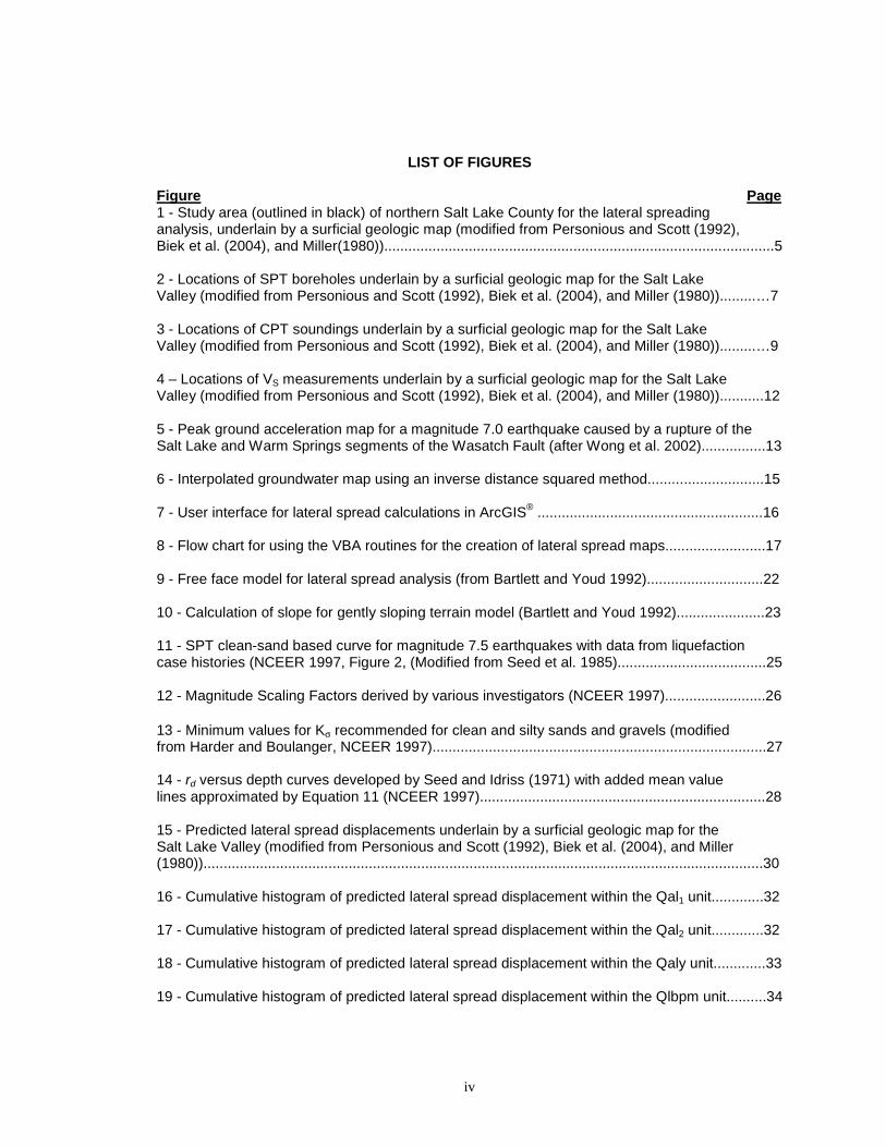
LIST OF FIGURES Figure Page 1 - Study area (outlined in black) of northern Salt Lake County for the lateral spreading analysis, underlain by a surficial geologic map (modified from Personious and Scott (1992), Biek et al. (2004), and Miller(1980)).................................................................................................5 2 - Locations of SPT boreholes underlain by a surficial geologic map for the Salt Lake Valley (modified from Personious and Scott (1992), Biek et al. (2004), and Miller (1980)).........…7 3 - Locations of CPT soundings underlain by a surficial geologic map for the Salt Lake Valley (modified from Personious and Scott (1992), Biek et al. (2004), and Miller (1980)).........…9 4 – Locations of VS measurements underlain by a surficial geologic map for the Salt Lake Valley (modified from Personious and Scott (1992), Biek et al. (2004), and Miller (1980))...........12 5 - Peak ground acceleration map for a magnitude 7.0 earthquake caused by a rupture of the Salt Lake and Warm Springs segments of the Wasatch Fault (after Wong et al. 2002)................13 6 - Interpolated groundwater map using an inverse distance squared method.............................15 7 - User interface for lateral spread calculations in ArcGIS® ........................................................16 8 - Flow chart for using the VBA routines for the creation of lateral spread maps.........................17 9 - Free face model for lateral spread analysis (from Bartlett and Youd 1992).............................22 10 - Calculation of slope for gently sloping terrain model (Bartlett and Youd 1992)......................23 11 - SPT clean-sand based curve for magnitude 7.5 earthquakes with data from liquefaction case histories (NCEER 1997, Figure 2, (Modified from Seed et al. 1985).....................................25 12 - Magnitude Scaling Factors derived by various investigators (NCEER 1997).........................26 13 - Minimum values for Kσ recommended for clean and silty sands and gravels (modified from Harder and Boulanger, NCEER 1997)...................................................................................27 14 - rd versus depth curves developed by Seed and Idriss (1971) with added mean value lines approximated by Equation 11 (NCEER 1997).......................................................................28 15 - Predicted lateral spread displacements underlain by a surficial geologic map for the Salt Lake Valley (modified from Personious and Scott (1992), Biek et al. (2004), and Miller (1980))...........................................................................................................................................30 16 - Cumulative histogram of predicted lateral spread displacement within the Qal1 unit.............32 17 - Cumulative histogram of predicted lateral spread displacement within the Qal2 unit.............32 18 - Cumulative histogram of predicted lateral spread displacement within the Qaly unit.............33 19 - Cumulative histogram of predicted lateral spread displacement within the Qlbpm unit..........34

v

20 - Cumulative histogram of predicted lateral spread displacement within the northern portion of the Qlaly unit..................................................................................................................35 21 - Cumulative histogram of predicted lateral spread displacement within the southern portion of the Qlaly unit..................................................................................................................36 22 - Cumulative histogram of predicted lateral spread displacement for the south-western portion of the lacustrine deposits (Qlaly and Qly) on the west side...............................................37 23 - Lateral spreading hazard map for the Northern Salt Lake County based on a Magnitude 7.0 earthquake...............................................................................................................................38 24 - Sample seismic hazard curve.................................................................................................40 25 - Schematic illustration of conditional probability of DH exceeding a threshold of x for a given magnitude, distance, and acceleration (modified from Kramer 1996, p. 126)......................42 26 - Soil-type distribution for the Qal1 geologic unit based on 137 samples..................................62 27 - N160 blow-count distribution for the Qal1 geologic unit based on 89 granular samples..........62 28 - Plastic-index distribution in the Qal1 geologic unit based on 13 fine soil samples..................63 29 - Soil-type distribution for the Qal2 geologic unit based on 245 samples..................................63 30 - N160 blow-count distribution for the Qal2 geologic unit based on 146 granular samples........64 31 - Plastic-index distribution for the Qal2 geologic unit based on 13 fine soil samples................64 32 - Soil-type distribution for the Qaly geologic unit based on 149 samples.................................65 33 - N160 blow-count distribution for the Qaly geologic unit based on 81 granular samples..........65 34 - Soil-type distribution for the Qalp geologic unit based on 70 samples...................................66 35 - N160 blow-count distribution for the Qalp geologic unit based on 52 granular samples.........66 36 - Soil-type distribution for the Qaf2 geologic unit based on 137 Samples.................................67 37 - N160 blow-count distribution for the Qaf2 geologic unit based on 89 granular samples..........67 38 - Plastic-index distribution in the Qaf2 geologic unit based on 10 fine soil samples.................68 39 - Soil-type distribution for the Qly geologic unit based on 26 samples.....................................68 40 - Plastic-index distribution in the Qly geologic unit based on 11 fine soil samples……....…….69 41 - Soil-type distribution for the Qlaly geologic unit based on 533 samples.................................69 42 - N160 blow-count distribution for the Qlaly geologic unit based on 110 granular samples...…70

vii 43 - Plastic-index distribution for the Qlaly geologic unit based on 79 fine soil samples.…......….70 44 - Soil-type distribution for the Qlpg geologic unit based on 97 samples...................................71

vi

45 - N160 blow-count distribution for the Qlpg geologic unit based on 89 granular samples......…71 46 - Soil-type distribution for the Qlbg geologic unit based on 100 samples.................................72 47 - N160 blow-count distribution for the Qlbg geologic unit based on 78 granular samples.........72 48 - Soil-type distribution for the Qlbs geologic unit based on 612 samples.................................73 49 - N160 blow-count distribution for the Qlbs geologic unit based on 301 granular samples........73 50 - Plastic-index distribution in the Qlbs geologic unit based on 29 fine soil samples.................74 51 - Soil-type distribution for the Qlbm geologic unit based on 176 samples................................74 52 - N160 blow-count distribution for the Qlbm geologic unit based on 10 granular samples….....75 53 - Plastic-index distribution in the Qlbm geologic unit based on 33 fine soil samples................75 54 - Soil-type distribution for the Qlbpg geologic unit based on 91 samples.................................76 55 - N160 blow-count distribution for the Qlbpg geologic unit based on 79 granular samples.......76 56 - Soil-type distribution for the Qlbps geologic unit based on 498 samples...............................77 57 - N160 blow-count distribution for the Qlbps geologic unit based on 294 granular samples......77 58 - Plastic-index distribution in the Qlbps geologic unit based on 36 fine soil samples...............78 59 - Soil-type distribution for the Qlbpm geologic unit based on 5035 samples............................78 60 - N160 blow-count distribution for the Qlbpm geologic unit based on 414 granular samples....79 61 - Plastic-index distribution in the Qlbpm geologic unit based on 665 fine soil samples............79

vii

LIST OF TABLES

Table Page 1 - Correction factors for blow counts used in liquefaction analysis. (Modified from Youd et al. (2002), as modified from Skempton (1986))................................................................20 2 - Database structure for the SITE table......................................................................................44 3 - Database structure for the BLOW and BLOWFILL tables........................................................46 4 - Geologic unit symbols and descriptions...................................................................................51

viii

LIST OF SYMBOLS

Symbol Description A Peak ground acceleration, g

α

Coefficient for fines correction

amax Maximum ground acceleration at a site

β

Coefficient for fines correction

CB Correction for borehole diameter

CE Correction for hammer energy efficiency

CN Correction for overburden pressure

CR Correction for "short" rod length

CRR7.5 Cyclic resistance ratio for a magnitude 7.5 event

CS Correction for non-standardized sampler configuration

CSR Cyclic stress ratio

D50 Mean grain size (mm)

D50-15 Mean grain size, averaged over a liquefiable layer ((N1)60 < 15), mm

DH Predicted lateral spread, m

di Thickness of layer, m

F15 Fines content, averaged over a liquefiable layer ((N1)60 < 15), %

FC Fines Content, %

Fz(z) Cumulative Density Function (CDF) for the standard normal vairate, z

g Acceleration of gravity, 9.81 m/s2

Gs Specific Gravity

H Free-face height, m

i Layer number, and summation variable

Kσ Correction for overburden pressure

L Distance to free-face, m

LL Liquid limit, %

log Logarithm to the base 10

ix

M or Mw Earthquake Magnitude

MSF Magnitude scaling factor

Mw Earthquake magnitude

N Standard penetration blow-count

N160 Corrected standard penetration blow-count for a 60% energy ratio

N160-CS Corrected standard penetration blow-count for a 60% energy ratio and

corrected for fines content

P[A, M, R] Joint probability density function of peak ground acceleration (A), the earthquake magnitude (M), and the horizontal distance to the seismic source (R.)

P[A, M] Joint probability density function of peak ground acceleration (A) and the earthquake magnitude (M)

P[E] Probability of exceedance

P[DH>x] Probability of lateral spread exceeding a threshold value (x)

P[ DH > x) | L] Probability of lateral spread exceeding a threshold value (x) given liquefaction

PE[L] Annual probability of liquefaction for a given seismic event

P[L] Annual probability of liquefaction

P[L | A, M] Conditional probability of liquefaction given the peak ground acceleration (A) and the earthquake magnitude (M)

P[L | A, M, R] Conditional probability of liquefaction given the peak ground acceleration (A) and the earthquake magnitude (M) and the horizontal distance to the seismic source (R.)

P[NE] Probability of non-exceedance

Pa Atmospheric pressure (1atm = 1 tsf) , tsf

pga Peak ground acceleration, g

PI Plastic-index, %

PL Plastic limit, %

R Distance to seismic source (fault), km

R* Function of R and M used in prediction of lateral spread

rd(z) Depth reduction factor, a function of depth, z

S Slope of the ground, %

x

σlog(DH) Standard variation of the Youd et al. regression model (2002)

σv0 Total vertical stress (psf)

σ'v0 Effective vertical stress (psf)

T15 Thickness of the liquefiable layer ((N1)60 < 15), m

τav Cyclic shear stress

U Pore water pressure (psf)

VS 12m Shear wave velocity averaged over 12 m, m/s

VS 30m Shear wave velocity averaged over 30 m, m/s

vsi Shear wave velocity for the ith layer

W Free-face ratio (W = H/L), %

x Threshold lateral spread value, m

z Standard normal variate

z Depth

xii

xi

LIST OF ABBREVIATIONS

Abbreviation Definition AGRC Automated Geographic Regional Council

CDF Cumulative Distribution Function

CDMG California Division of Mines and Geology

COSMOS Consortium of Organizations for Strong-Motion Observation Systems

CPT Cone Penetrometer Testing

DEM

Digital Elevation Model

GIS Geographic Information Systems

IDW Inverse Distance Weighted

LPI Liquefaction Potential Index

LSI Liquefaction Severity Index

NAD North American Datum

NCEER National Center for Earthquake Engineering Research

NEHRP National Earthquake Hazards Reduction Program

SPT Standard Penetration Testing

U of U University of Utah

UGS Utah Geologic Survey

ULAG Utah Liquefaction Advisory Group

USGS United States Geologic Survey

USU Utah State University

UTM Universal Transverse Mercator

VBA Visual Basic for Applications

VS Shear Wave Velocity

xii

ACKNOWLEDGMENTS

I would like to acknowledge the financial assistance of the United States Geologic Survey (USGS) with the National Earthquake Hazards Reduction Program (NEHRP) Award 04HQGR0026 for the data collection. I would like to express appreciation to Dr. Steven Bartlett for his continual guidance and assistance in the production of this thesis. I would like to express gratitude for Barry Solomon for his assistance in the geologic coordination of the data to the mapping effort. In addition, I am grateful for the various people who contributed data for the project including Darlene Batanian of the Salt Lake City County Public Works, Greg McDonald of the Utah Geologic Survey, the Utah Department of Transportation, and Dave Simon of Simon-Bimaster Inc. The assistance of Griffen Ericksson with the collection of data in Southern Salt Lake County is appreciated. I would also like to acknowledge the assistance of Dr. Evert Lawton and Dr. James Pechmann for their comments in the review of this document.

1

INTRODUCTION

Liquefaction occurs in loose, water-saturated sand and non-plastic silt soils. As the soil experiences cyclic loading during strong motion, these soils lose shear strength due to high pore water pressure. This loss of strength causes the soil to behave more like a liquid than a solid, resulting in various catastrophic problems such as flow failure, lateral spreading, differential settlement, bearing capacity failure, and ground oscillation. These ground failures can cause significant damage and/or collapse of bridges, buildings, and roadways, which can also lead to loss of human life.

Lateral spreading occurs when a soil liquefies and moves horizontally during a seismic event. This type of ground failure has caused substantial damage during several large earthquakes, notably during the 1964 Nigata Earthquake in Japan. For this reason, researchers have developed methods to estimate the amount of lateral spreading that will occur in loose, saturated granular deposits. The method used in this pilot study area was the Bartlett-Youd lateral spreading regression equations (Bartlett and Youd 1992) with updated regression coefficients developed based on a larger database (Youd et al. 2002).

Types of Liquefaction Mapping

Because of the high damage caused by liquefaction ground deformation, various

liquefaction maps have been created throughout the United States (Power and Holzer 1996). Some of these maps are historical liquefaction maps created based on historical occurrences of liquefaction; although there are relatively few of these historical maps. The most common type of maps, liquefaction hazard maps, divide a region into smaller areas based on varying degrees of liquefaction hazard. These maps can be divided into three subcategories: liquefaction susceptibility maps, liquefaction potential maps, and liquefaction-induced ground failure maps.

Liquefaction Susceptibility Maps

The first type of maps, the liquefaction susceptibility maps, analyzes the liquefaction hazard using several types of data including geologic mapping, historical liquefaction information, groundwater depth, and soil boring data (Standard Penetration Testing (SPT) and Cone Penetrometer Testing (CPT)). These maps delineate between low, moderate, and high susceptibility of liquefaction. Some maps have additional categories such as very low or very high. These maps do not account for a specific seismic source or the occurrence rate of the seismicity.

Liquefaction Potential Maps

The second type of maps, liquefaction potential maps, incorporates the liquefaction

susceptibility map with the earthquake potential in a region. These maps show expected liquefaction from a selected regional scenario earthquake, the likelihood of liquefaction during a certain time period (i.e. 10% occurrence probability in a 50-year period), or a return period (i.e. 1 event in 500 years) of liquefaction. These maps correlating geologic conditions with levels of seismic shaking were developed by Youd and Perkins (1978) by merging two maps. The first map consists of a ground failure opportunity map developed based on the seismicity of the area and the occurrence rate of ground motions substantial enough to induce liquefaction. This map calculates the predictive earthquake ground motion based on the expected earthquake magnitude and the distance from the fault. The second map, a ground failure susceptibility map, shows the susceptibility of geologic materials and the likelihood of those materials liquefying and laterally spreading during an earthquake. Youd and Perkins (1978) determined the susceptibility of the soils by classifying the hazard according to the type and age of the deposits. Also, in determining the susceptibility of those deposits, they incorporated the influence of groundwater depths by assigning areas with deep groundwater depths a low hazard. They then merged the

2

ground failure opportunity and ground failure susceptibility maps to produce liquefaction potential maps.

The State of California has developed several liquefaction maps based on the Youd and Perkins (1978) mapping techniques. For many of those mapping efforts, only qualitative information was available and more studies were required to quantify the hazard. Thus, those maps were meant to provide a preliminary classification of the hazard but were unable to quantify its extent. To improve those maps by quantification, the State of California utilizes a universal geotechnical database developed by the Consortium of Organizations for Strong-Motion Observations Systems (COSMOS), in which data can be input and shared via the internet (PEER 2001). The XML language used for the database makes it particularly effective to run via the internet where many users can access the database and input their data or query the existing data and use it for various analyses. Liquefaction researchers currently use these data to create maps by calculating acceleration values required to induce liquefaction and comparing that to what has been predicted in the area (DeLisle 2000).

Liquefaction Ground Failure Maps

The third type of maps, the liquefaction ground failure maps, then build upon the liquefaction potential map and attempt to characterize the permanent ground deformation associated with liquefaction. These maps can be based on scenario earthquakes or on probabilistic analysis. The most common type of these maps is the Liquefaction Severity Index (LSI) which estimates the maximum amount of ground displacement based on lateral spreading in gently sloping, liquefaction-susceptible deposits and incorporates that into the hazard. This mapping technique was developed by Youd and Perkins (1987).

Many techniques of liquefaction ground failure maps recognize that the thickness of the liquefiable layer plays a significant role in the amount of post-liquefaction settlement, the horizontal displacement caused by lateral spreading, and the amount of earthquake damage to buried pipelines. O’Rouke and Pease (1997) mapped the thickness of liquefiable layers in the San Francisco Bay area using both SPT and CPT data. In their analysis, they first determined the submerged thickness of liquefaction susceptible soils. Second, they then converted this thickness to a maximum liquefiable thickness by determining the maximum thickness of soil that would experience liquefaction with extreme ground motion. Third, they calculated the net liquefiable thickness by subtracting out clay and silt layers of the submerged deposit. Fourth, they predicted if the deposits would liquefy for a given level of earthquake intensity. Lastly, O’Rouke and Pease (1997) then mapped the thicknesses of these deposits to show what areas would be anticipated to have the largest post-liquefaction effects.

Liquefaction Potential Index (LPI) maps (Toprak and Holzer 2003) take into account the thickness of the liquefiable layer, the proximity of that layer to the ground surface, and the factor of safety against liquefaction predicted. These factors are then combined with surficial geologic maps where LPI contours are drawn within each unit. By better describing the liquefaction hazard by weighting areas by their thickness and proximity to the surface, it shows what areas would be expected to experience more damage from liquefaction. Thus, this method offers some advantages to a purely deterministic yes/no evaluation of the liquefaction hazard. It, however, does not quantify the amount of displacement expected.

Previous Mapping Efforts in Utah

The potential for liquefaction-induced ground failure has become a major concern along

the Wasatch Front because of its inherent potential for large earthquakes and a substantial amount of loose sand and sandy-silt deposited in the adjacent valleys. The effort to develop liquefaction hazard maps in Utah began in 1980 when Utah State University received a NEHRP grant to complete a study for Davis County (Anderson et al. 1982). They collected a large amount of Standard Penetration Test (SPT) data with blow counts and used this data to determine the liquefaction susceptibility of the soil deposits. The acceleration values to trigger

3

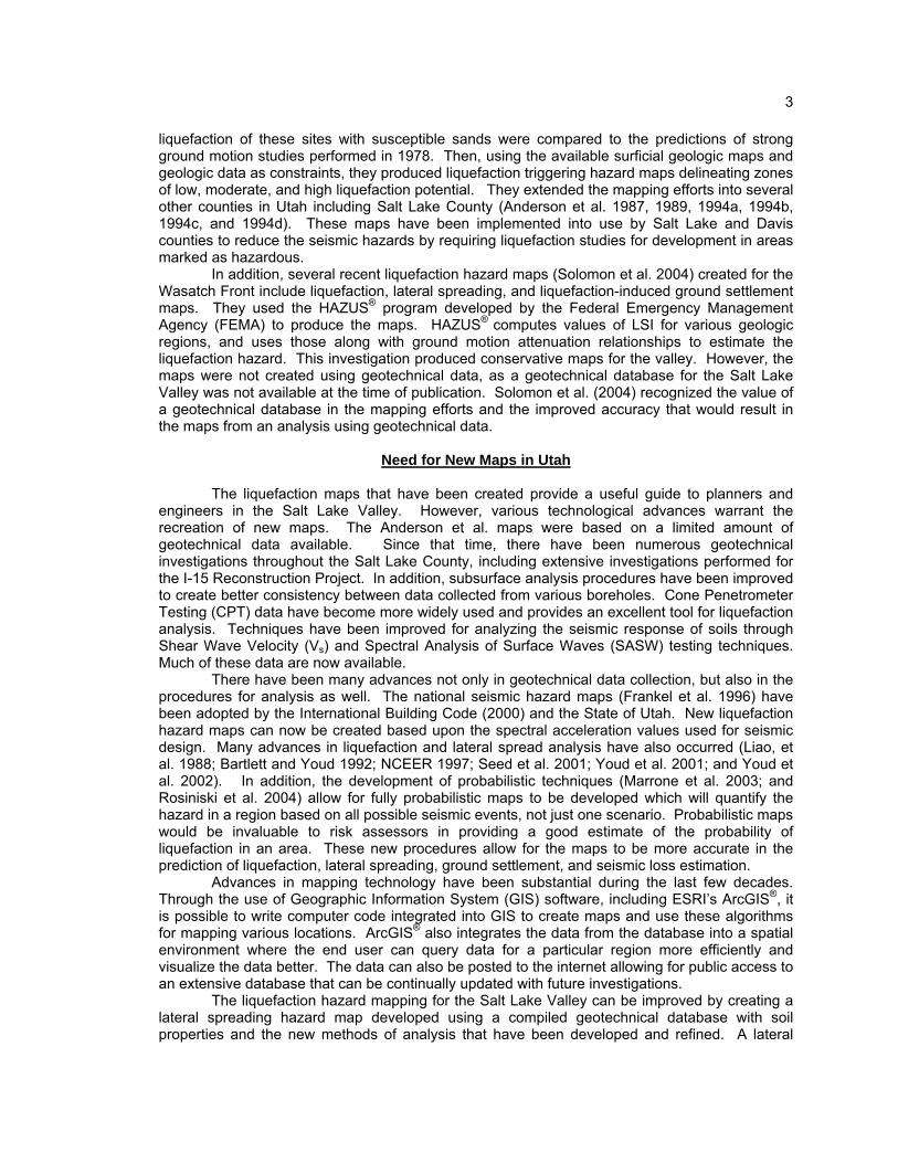
liquefaction of these sites with susceptible sands were compared to the predictions of strong ground motion studies performed in 1978. Then, using the available surficial geologic maps and geologic data as constraints, they produced liquefaction triggering hazard maps delineating zones of low, moderate, and high liquefaction potential. They extended the mapping efforts into several other counties in Utah including Salt Lake County (Anderson et al. 1987, 1989, 1994a, 1994b, 1994c, and 1994d). These maps have been implemented into use by Salt Lake and Davis counties to reduce the seismic hazards by requiring liquefaction studies for development in areas marked as hazardous. In addition, several recent liquefaction hazard maps (Solomon et al. 2004) created for the Wasatch Front include liquefaction, lateral spreading, and liquefaction-induced ground settlement maps. They used the HAZUS® program developed by the Federal Emergency Management Agency (FEMA) to produce the maps. HAZUS® computes values of LSI for various geologic regions, and uses those along with ground motion attenuation relationships to estimate the liquefaction hazard. This investigation produced conservative maps for the valley. However, the maps were not created using geotechnical data, as a geotechnical database for the Salt Lake Valley was not available at the time of publication. Solomon et al. (2004) recognized the value of a geotechnical database in the mapping efforts and the improved accuracy that would result in the maps from an analysis using geotechnical data.

Need for New Maps in Utah

The liquefaction maps that have been created provide a useful guide to planners and engineers in the Salt Lake Valley. However, various technological advances warrant the recreation of new maps. The Anderson et al. maps were based on a limited amount of geotechnical data available. Since that time, there have been numerous geotechnical investigations throughout the Salt Lake County, including extensive investigations performed for the I-15 Reconstruction Project. In addition, subsurface analysis procedures have been improved to create better consistency between data collected from various boreholes. Cone Penetrometer Testing (CPT) data have become more widely used and provides an excellent tool for liquefaction analysis. Techniques have been improved for analyzing the seismic response of soils through Shear Wave Velocity (Vs) and Spectral Analysis of Surface Waves (SASW) testing techniques. Much of these data are now available.

There have been many advances not only in geotechnical data collection, but also in the procedures for analysis as well. The national seismic hazard maps (Frankel et al. 1996) have been adopted by the International Building Code (2000) and the State of Utah. New liquefaction hazard maps can now be created based upon the spectral acceleration values used for seismic design. Many advances in liquefaction and lateral spread analysis have also occurred (Liao, et al. 1988; Bartlett and Youd 1992; NCEER 1997; Seed et al. 2001; Youd et al. 2001; and Youd et al. 2002). In addition, the development of probabilistic techniques (Marrone et al. 2003; and Rosiniski et al. 2004) allow for fully probabilistic maps to be developed which will quantify the hazard in a region based on all possible seismic events, not just one scenario. Probabilistic maps would be invaluable to risk assessors in providing a good estimate of the probability of liquefaction in an area. These new procedures allow for the maps to be more accurate in the prediction of liquefaction, lateral spreading, ground settlement, and seismic loss estimation.

Advances in mapping technology have been substantial during the last few decades. Through the use of Geographic Information System (GIS) software, including ESRI’s ArcGIS®, it is possible to write computer code integrated into GIS to create maps and use these algorithms for mapping various locations. ArcGIS® also integrates the data from the database into a spatial environment where the end user can query data for a particular region more efficiently and visualize the data better. The data can also be posted to the internet allowing for public access to an extensive database that can be continually updated with future investigations.

The liquefaction hazard mapping for the Salt Lake Valley can be improved by creating a lateral spreading hazard map developed using a compiled geotechnical database with soil properties and the new methods of analysis that have been developed and refined. A lateral

4

spreading map has advantages over a liquefaction potential map because the former shows estimated displacement, and thus, how much damage might occur when liquefaction occurs. This information allows engineers to plan and design for the liquefaction hazard and its extent.

PROCEDURES

To produce a lateral spreading hazard map, several phases of work needed to be completed. The first phase involved data collection for the Salt Lake Valley, concentrating on SPT and CPT testing. The second phase involved writing computer routines within the Visual Basic for Applications (VBA) Editor in ArcGIS® to process the subsurface data. The third phase consisted of analyzing the data output of the computer routines with the surficial geology to better map the lateral spreading hazard. The study area for this pilot project and surficial geology are shown in Figure 1.

Phase 1: Data Collection

Several factors influenced the data collection throughout the pilot project area. Of the available data, the collection efforts were prioritized to input the highest quality data available and to have it distributed as uniformly as possible across the study region. The three most important factors influencing the collection of data include:

1. Data quality - The data were screened and given data quality indicators to ensure that the boring was of adequate depth to capture all potentially liquefiable layers, that quality laboratory and on-site investigations were performed, and that the borings were well documented, reducing the uncertainty for the analysis. 2. Adequate sampling of each geologic unit - Sufficient boreholes were collected to provide an adequate representation of each surficial geologic unit, so that the geotechnical and geologic data could be reasonably correlated. 3. Spatial distribution of boreholes - The spatial distribution of the boreholes needed to be considered so that changes in extensive geologic units could be adequately modeled in the mapping process.

Unfortunately however, it was not always possible to use the highest level of data quality for the analysis. As will be discussed later, by recording the quality of the data in the database, future projects can identify data of lower quality and quantify uncertainty. The data collected for this pilot project were obtained from several sources. Data from previous site-specific liquefaction studies were obtained from the Salt Lake County Government. Data from highway investigations by the Utah Department of Transportation (UDOT) were used extensively, as well. These data include borehole logs for the older Interstate 80 (I-80) and Interstate 215 (I-215) construction projects. The Interstate 15 (I-15) Reconstruction Project subsurface data composes an extensive portion of the database. This I-15 data, available in electronic format (GINT® database), allowed for a more rapid transfer of data to the ArcGIS®

database. The borings used by Anderson et al. in their previous mappings, obtained from the Utah Geological Survey (UGS), filled in gaps where there was limited data available from more recent investigations. Some geotechnical consultants also assisted by providing data for the mapping effort. These data, in combination, allow sufficient sampling of each geologic unit and spatial distribution to produce the map.

5

6

To organize the data collected a geodatabase structure was used within ArcGIS®

creating several feature classes for each type of data. A copy of this database resides in the file liquefaction database.mdb, included on the enclosed disk. This database utilizes a Microsoft® Access database to store the data and spatial information, allowing for ease of data manipulation and querying by those who have access to ArcGIS® and Microsoft® Office. If ArcGIS® is not available, the data can still be edited using Microsoft® Access as tables without the use of ArcGIS®. The database consists of several feature classes and tables. These include the SITE, SITECPT, and VS feature classes which contain information about the sites where data has been collected. The tables include the BLOW, CPTDATA, and footnote tables which contain the sampling data. The contents of each of these tables will be discussed individually. The database has been set up with the same field names and types as the COSMOS database for better compatibility with other mapping projects that are being undertaken.

Standard Penetration Testing (SPT) Data

SPT data obtained from over 800 borings was stored in two tables: SITE and BLOW.

These tables are linked through a one to many relationship established in Microsoft Access® by a site identification number (SITEIDNO). For each borehole and its unique site identification number, there are several records in the BLOW table representing each sample in the borehole. Also, the BLOW table has records that identify the depth to the layer boundaries. The structure and field names of these tables can be found in Appendix A.

The SITE table contains the information about the borehole site, including the important parameters of the location, groundwater depth, type of equipment used, and information regarding the source of the borehole data. One field in the SITE table contains a hyperlink to a PDF file showing a scanned image of the original boring log for inspection and review. Figure 2 shows a plot of the SPT boreholes input in the database.

The BLOW table contains the properties of the soil obtained at various sampling depths for each borehole recorded in the SITE table. Such information includes the depth of the sampling, type of sampler and its properties, soil description and its Unified Soil Classification System (USCS) classification, uncorrected SPT blow count (NM), dry unit weight (DRYUNIT), moisture content (MOISTURE_CONTENT), fines content (FINES), which is the percent finer than the No. 200 standard sieve, mean grain size (D50), and Atterberg limits, where applicable.

For samples where data were not available for all data fields, several methods were used to fill in data gaps. Because the quality and extent of data available varies, due to its varied sources, estimates were made to fill in data gaps. To keep track of estimated properties, a system of data qualifiers was implemented. The SITE and BLOW tables include data qualifier fields for each important field ranking the data from 1 to 3. A “1” is given to data collected and recorded in the originating report. A “2” is given to the data that could be reasonably estimated from other samples in the same borehole or nearby borehole logs. A “3” denotes data estimated from another source. The BLOW table also includes two additional data qualifiers of “4” and “5”. A “4” denotes that average values were used from the same soil type from the same geologic unit and a “5” indicates that the average values were from the same soil type, but not necessarily from the same geologic unit. These averages filled in data gaps, as necessary, but were not used to estimate penetration resistances. To ensure an accurate liquefaction triggering analysis, only original data were used for penetration resistances.

7

8

A footnote table, included in the database, contains information regarding data sources

and information about the data obtained from nearby boreholes. This process, described above, fills in the database with better estimates than simply averaging from the entire dataset and allows for future researchers to replace the estimated values, so if better data became available, the database can be adapted. The data qualifiers will also allow for a more rigorous assessment of uncertainty in subsequent probabilistic evaluations. Uncertainty evaluations have been requested by the USGS and will be completed with future probabilistic liquefaction hazard mapping, but were not completed as part of this study.

The typical values table, developed later during the data collection, contains information of the typical properties of equipment used by drilling companies. In the event that a boring log is missing information about the equipment used in a particular site investigation, the user can use the typical values table to provide an estimate of the typical equipment used by a specific company to fill in data gaps, as necessary.

Cone Penetrometer Testing (CPT) data

In addition to the SPT data, Cone Penetrometer Testing (CPT) data collected from approximately 400 cone penetrometer soundings was imported into the liquefaction database. Figure 3 shows the locations of these CPT soundings. Unfortunately, the CPT soundings were not as well-distributed spatially as the SPT boreholes because of the limited amount of CPT investigations in the valley. Much of these data were collected from heavy sampling in the center of the valley for the I-15 Reconstruction Project. Additional CPT data were collected from the Kennecott Tailings Pond investigations and from the Salt Palace Expansion Investigation. Other CPT soundings were collected from various ConeTech Investigations across the Salt Lake Valley compiled by Utah State University (Bischoff 2005).

The data for these CPT soundings were organized in two tables in the liquefaction database: the SITECPT and CPTDATA tables. The SITECPT table contains the coordinates of the site and other general information about the CPT soundings, similar to the information found in the SITE table for the SPT data. The CPTDATA table contains continuous sampling information, including the depths in meters (DEPTHM), the uncorrected tip stress in kilopascals (QUNC), the sleeve friction in kilopascals (SLEEVE), and the pore water pressure in kilopascals (PPRESSURE) at each recorded depth for the CPT soundings. This table is very similar in function to the BLOW table for SPT data.

For thinly bedded deposits, the CPT provides a better investigation of liquefaction susceptibility due to its ability to distinguish smaller sand interbeds from clayey soils that can easily be missed in a SPT sampling interval. Unfortunately, the CPT data were not used in the lateral spread analysis for the study area, because there was not sufficient spatial distribution of CPT data to produce lateral spreading maps. Also, lateral spread analysis requires estimates of the fines content and the mean grain size (D50) of the sandy soils, which cannot be directly estimated from CPT data. These properties must be inferred from site-specific empirical correlations, which do not currently exist for the Salt Lake Valley. However, these correlations will be produced in a future study from many paired SPT and CPT drill holes along the I-15 corridor, which have been input into the liquefaction database as part of this project. These correlations will allow for the CPT data to be used in future liquefaction and lateral spread mapping projects.

9

10

The fact that CPT data were not used does not greatly impact this study. Most of the

CPT soundings gathered are located along the I-15 corridor where abundant SPT data already exist. Thus, the CPT data are essentially redundant data for this investigation. Future mapping will also evaluate the consistency of CPT and SPT methods, using data from the I-15 Reconstruction and Legacy Highway Construction Projects.

Shear Wave Velocity (VS) Data

Part of the project funded by NEHRP requires the generation of probabilistic liquefaction triggering maps, which require estimates of shear wave velocities (Seed et al. 2001). The ArcGIS® routines to complete these analyses are currently being developed by researchers from Utah State University (USU). These data were compiled by this project, but the analyses will be completed by USU.

The VS table contains the shear wave velocity (Vs) data collected by the Utah Geologic Survey (Ashland and Rollins 1999) and Utah State University (Bischoff 2005) and entered into the ArcGIS® database. It contains VS measurements averaged over a 30 m (100 ft) interval (VS-30m) and VS measurements averaged over a 12 m (40 ft) interval (VS-12m). The VS-30m measurements are used for site classification purposes, and the VS-12m measurements are necessary for computing the liquefaction depth reduction factor (rd) using the methods of Seed et al. (2001). From the work of Ashland and Rollins (1999) and Bischoff (2005), the VS-30m values were already computed. VS-12m measurements were computed from the raw VS data according to the following equation, which is the same as the equation used for calculating VS-30m, only it is calculated over a 12 m interval rather than 30 m.

∑

∑

=

=− = n

i si

i

n

ii

s

vd

dV

1

112

[Eq. 1]

where: Vs-12m = the average shear wave velocity in the upper 12 meters of a

CPT sounding, di = the thickness of a layer i in the CPT sounding and vsi = the shear wave velocity of layer i.

The sites with shear wave velocity measurements and averages of VS-30m and VS-12m can be found in the liquefaction database.mdb file on the attached disk in the VS table. Figure 4 shows the locations of these shear wave velocity measurements. These Vs measurements can be assigned to the boreholes in the SITE feature class based on the closest Vs measurement within the same geologic unit via the VSFinder routine (See Appendix C).

Geologic Mapping Data

Because the project combines both geologic and geotechnical data to produce the map, it is important to adequately represent geologic units as best possible. The geologic mappingwas done using various existing maps merged to create a surficial geologic map for the northern part of Salt Lake County (See Figure 1). The surficial geologic map by Personious and Scott (1992) was used for the eastern part of the county. By scanning and digitizing this map into a polygon feature class in a geodatabase, it could be used programmatically. Biek et al. (2004) recently mapped the geology of the Magna Quad. However, the north-western and western portions of Salt Lake County had not recently been mapped. For this area, extrapolations of geologic units

11

from the boundaries of previously mapped areas were used where current maps were not available. The older geologic mapping by Miller (1980) provided a reasonable reference and guide to map that area, as well.

Descriptions of the mapped geologic units can be found in Appendix B. These descriptions were modified from Personious and Scott (1992) and Biek et al. (2004) because the maps used different geologic descriptions for some of the same units. In addition, Appendix B contains histograms based on the sampling input in the database for each extensive geologic unit with substantial sampling. Histograms of soil type, corrected blow counts (N160) of granular soils, and plastic-index values for cohesive soils are included for these units. These histograms provide a useful, quantitative idea of the general engineering properties of the soils within these geologic units in the Salt Lake Valley.

The coordination of geotechnical data with the surficial geologic mapping assisted in mapping geologic units where the data where the data was sparse in comparison to others. Although, the geotechnical data was not crucial in most of these units because they are located in areas insusceptible to liquefaction because of a deep groundwater table, it allowed for the inference of properties in areas without much data where the groundwater was shallow and the soils were potentially liquefiable.

Miscellaneous Data and Analyses

Although this study focused on lateral spread mapping, a deterministic liquefaction triggering analysis was completed for the mapped area. This triggering analysis was done to verify that liquefaction would indeed be triggered in the borehole prior to estimating the amount of lateral spread. For this triggering analysis, peak ground acceleration estimates are required. The estimates were obtained from an ArcGIS® grid file containing peak ground acceleration (pga) values gridded at a spacing of 30 m along the Wasatch front (Wong et al. 2002), as shown in Figure 5. Wong et al. (2002) mapped surface soil estimates of pga from a magnitude 7.0 earthquake on the Salt Lake City and Warm Springs segments of the Wasatch fault

The lateral spread equations of Bartlett and Youd (1992) and Youd et al. (2002) require estimates of the ground slope, or the height of a free-face, when present. For the lateral spread routines, digitized elevation data was necessary to calculate ground slopes. This data was obtained from the national elevation dataset hosted by the USGS (http://seamless.usgs.gov/). The best available grid for the region was the 1/3 Arc-Second grid which contained elevations gridded at a 9 meter spacing. By having a continuous data grid, ground slopes could be calculated at each of the borehole locations. These methods are discussed later in the Visual Basic routines.

For the free-face lateral spread model, an ArcGIS® shapefile containing geographic information of various rivers and canals in Salt Lake was obtained from the Automated Geographic Regional Council (AGRC). The locations of the free faces used in the analysis are shown by the rivers in blue in Figures 1 - 4. With the addition of a depth field to the shapefile, the routines can read off the average depth of that feature and use that depth to calculate the free face value, W, used in the lateral spread regression equation. These depths were calculated by averaging survey cross sections of these rivers and channels obtained from Salt Lake County Public Works.

12

.

S

13

Salt Lake City Segment

Warm Springs Segment

14

To determine the horizontal distance from the site to the fault, R (km), a GIS Shapefile of

the Salt Lake City and Warm Springs segments of the Wasatch Fault was obtained from the AGRC, which uses polylines to show the locations of the faults. These faults are shown in black on Figure 5. The dashed lines indicate inferred faults.

A GIS shapefile of the Great Salt Lake, obtained from the AGRC as well, was used to map the location of the Great Salt Lake based on the elevation of the lake. The Great Salt Lake was mapped at its average twentieth century elevation of 4200 ft.

Groundwater Data

For a soil to be liquefiable, it must be saturated, and thus, groundwater depth is crucial for the liquefaction and lateral spread analyses. A recent and reliable groundwater map is not available for the Salt Lake Valley. To remedy this situation, the groundwater depths recorded in the boreholes were used to create an interpolated groundwater map using ArcGIS® Spatial Analyst and an inverse distance weighted method. The results of this interpolation are shown in Figure 6. The darker blue values represent shallower groundwater and the lighter colors represent deeper groundwater depths. The results of this map are only utilizable in the valley because there are very few data points collected up in the bench and foothill areas. Fortunately, for this project, most of the data points missing groundwater information are located within the valley, so this is not an issue.

The groundwater query routine (See Appendix C) assigns an estimate of groundwater depth to each borehole without a recorded groundwater depth. This routine reads values from the groundwater grid map. This routine is further explained later in this document. To add some conservatism to cover the uncertainty associated with the groundwater depth because it fluctuates substantially during the year and from year to year, the routines perform the analysis using groundwater elevations that are 5 ft higher than those recorded in the boreholes or those predicted by the interpolation map. If this conservatism put the groundwater depth above the ground surface, a value of 0 ft was used for the groundwater depth. In addition, if part of a sand layer was saturated, it was assumed that the entire layer was saturated for the analysis.

Phase 2: Visual Basic for Application Routines for Analysis.

To efficiently process the large amount of data collected for the analysis, several routines

were written using the Microsoft Visual Basic for Applications (VBA) Editor in ArcGIS®. These routines were written so as to be easily applied to future datasets collected for other mapping projects. Figure 7 shows a typical user interface developed within GIS where these tools can be accessed. The routines were set up as several smaller programs so that the user can evaluate the results after each step to ensure that error does not propagate. The user also can skip steps which do not need to be run for their particular dataset. These routines are not meant to be run blindly without the judgment and understanding required to properly perform a liquefaction analysis. They are designed to assist in speeding up the calculations so that more time can be spent in reviewing and interpreting the results. A flow chart summarizing the sequence to perform the analysis can be found in Figure 8. The following paragraphs describe these routines and the functions they perform.

15

16

Figure 7 - User interface for lateral spread calculations in ArcGIS®

17

Figure 8 - Flow chart for using the VBA routines for the creation of lateral spread maps

3. Run Average Calculator (creates an Average Table)

Missing data (Unit Weights, Gs, Fines Content, D50, Atterberg Limits)?

2. Copy BLOW table and name it BLOWFILL

4. Put estimates of fines content into the Average Table where there are none for the ALL geologic unit soil types

5. Run Average Filler (requires the table BLOWFILL)

Groundwater information available at all boreholes?

Groundwater Map available?

6. Use best interpolator in ArcGIS Spatial Analyst to create a groundwater grid (C:\liq\gwgrid).

8. Run Groundwater Query (requires gwgrid)

9. Run Total and Effective Vertical Stress Calculator Routine

Blow Counts already corrected to N160’s?

10a. Run N160 Calculator

11. Run LiqScreener to eliminate non-liquefiable soils.

10b. Rename NM field to N160

12. Run W Finder for the Free Face Model (requires a River shapefile with a depth field)

13. Create a Local Slope Grid using ArcGIS Spatial Analyst (C:\liq\slopegrid)

14. Run the SlopeFinder routine (requires DEM, Slopegrid)

15. Run the R Finder routine to calculate R (requires a Fault polyline shapefile)

16. Run Acceleration Reader (requires strong ground motion acceleration map in g’s)

17. Run Atrigger to calculate acceleration required for liquefaction

18. Run Layer Merger (15 Calculator)

19. Run Lateral Spread Calculator

1. Compile Data into Liquefaction Database.mdb (SITE and BLOW Tables) and collect grids (DEM, acceleration, and groundwater depths) and shapefiles (rivers.shp and fault.shp) into C:\liq\

Yes

Yes

Yes No

No

No Yes

No

20. Create Map based on results, groundwater levels, and surficial geologic data

18

Average Calculator

This program calculates averages of soil unit weights, fine contents, and mean grain sizes of the input data based on soil type and geologic unit and stores them in an average value table. For clayey soils, it calculates averages of the Atterberg Limits including the plastic limit, liquid limit and plastic index. It reads the BLOW table from the ArcGIS® database and only takes averages of properties with a data qualifier of “1”. Only these records are used so that only the highest quality data are used to create the averages. It first cycles through the entire BLOW table and calculates averages for each soil type within each geologic unit. It then cycles once again and calculates averages for each soil type regardless of the geologic unit. Thus, if some geologic units are lacking in data, a reasonable estimate can be made for the appropriate soil type. For each average value, the table shows how many records were averaged for that value to make it easier to spot outlying values which may be based on only a few records, allowing more flexibility for the user to determine how extensive the data needs to be to obtain a reliable average value.

Average Filler

Following the calculation of the average values, the average value procedure uses the average value table to fill in data gaps in a copy of the BLOW table called BLOWFILL. The user must manually create a copy of the BLOW table and rename it as the BLOWFILL table before running this procedure. It is also suggested that the user review and edit the average value table to verify that the results are reasonable before running this procedure. In order for all other procedures to run correctly, each soil type requires an estimate of the fines content. Thus, it is recommended to input estimates or typical values of the fines content in the average table for the various soil types averaged from ALL geologic units before continuing with this procedure. To keep track of the quality of the data, a data qualifier of “4” is given for average values based on the same soil type and the same geologic unit placed into the table. A data qualifier of “5” is used for average values that only come from the same soil type averaged among all geologic units. The program also puts in default values of specific gravity for soils using typical values of 2.65 for sandy soils, 2.70 for silty soils and 2.75 for clayey soils.

Groundwater Query

The groundwater query routine fills in the database with estimated values of groundwater depth. If accurate groundwater levels at every borehole exist, the routine can be skipped. Prior to running the routine, the user should create an interpolated groundwater grid using ArcGIS® Spatial Analyst, Geostatistical Analyst or similar method and verify its accuracy, if no groundwater map is available. An inverse distance weighted (IDW) method provided a reasonable interpolation for the Salt Lake Valley. In comparison to interpolations by Kriging and Spline interpolation methods, the IDW method tended to produce better results for the study area. This grid should be in the same coordinate system as the coordinates used for the SITE feature class. The program reads the grided groundwater values from the groundwater map based on the site location and fills in the missing values in the DEPTHGW field. A data qualifier of “3” is given for the groundwater depth estimate.

Total and Effective Vertical Stress Calculator

Once the groundwater level is input, total and effective vertical stress values can be calculated for each sampling interval recorded in the BLOW table. This program inputs the SITE table and the BLOW table and sorts the table by its site identification number and depth. It then reads in the dry unit weights, moisture contents, and specific gravities to calculate the wet unit weight and saturated unit weight. If values are not available in the database, the program assumes a dry unit weight of 15 kN/m3, a moisture content of 20%, and a specific gravity of 2.70, as a last resort, so that the program can continue to calculate all the values in a profile.

19

The total vertical stresses are calculated based upon the moist unit weight above the water table and the saturated unit weight below the groundwater table. The unit weights are assumed constant to a depth halfway between the current record and the next deepest record or constant between the sample in a layer and the nearest layer boundary. The pore-water pressure is calculated based on the depth to groundwater and is subtracted from the total vertical stress to calculate the effective vertical stress.

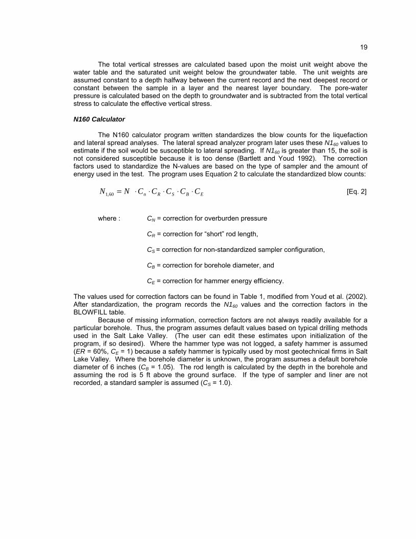
N160 Calculator

The N160 calculator program written standardizes the blow counts for the liquefaction and lateral spread analyses. The lateral spread analyzer program later uses these N160 values to estimate if the soil would be susceptible to lateral spreading. If N160 is greater than 15, the soil is not considered susceptible because it is too dense (Bartlett and Youd 1992). The correction factors used to standardize the N-values are based on the type of sampler and the amount of energy used in the test. The program uses Equation 2 to calculate the standardized blow counts:

EBSRn CCCCCNN ⋅⋅⋅⋅⋅=60,1 [Eq. 2]

where : CN = correction for overburden pressure CR = correction for “short” rod length, CS = correction for non-standardized sampler configuration,

CB = correction for borehole diameter, and

CE = correction for hammer energy efficiency.

The values used for correction factors can be found in Table 1, modified from Youd et al. (2002). After standardization, the program records the N160 values and the correction factors in the BLOWFILL table.

Because of missing information, correction factors are not always readily available for a particular borehole. Thus, the program assumes default values based on typical drilling methods used in the Salt Lake Valley. (The user can edit these estimates upon initialization of the program, if so desired). Where the hammer type was not logged, a safety hammer is assumed (ER = 60%, CE = 1) because a safety hammer is typically used by most geotechnical firms in Salt Lake Valley. Where the borehole diameter is unknown, the program assumes a default borehole diameter of 6 inches (CB = 1.05). The rod length is calculated by the depth in the borehole and assuming the rod is 5 ft above the ground surface. If the type of sampler and liner are not recorded, a standard sampler is assumed (CS = 1.0).

20

Table 1 - Correction factors for blow counts used in liquefaction analysis. (Modified from Youd et al. (2002), as modified from Skempton (1986))

Recommended Used

Factor Equipment Variable Correction Correction

CN - Overburden Pressure - CN = 2.2/(1.2+s'vo/Pa) CN = 2.2/(1.2+s'vo/Pa) - CN ≤ 1.7 CN ≤ 1.7 CE - Energy Ratio Safety hammer 0.5-1.0 0.75 Donut hammer 0.7-1.2 1.00 Automatic-trip hammer 0.8-1.3 1.33 CB - Borehole Diameter 65 - 115 mm 1.00 1.00 150 mm 1.05 1.05 200 mm 1.15 1.15 CR – Rod Length < 3 m 0.75 0.75 3-4 m 0.80 0.80 4-6 m 0.85 0.85 6-10 m 0.95 0.95 10-30 m 1.00 1.00 >30 m - 1.00 CS - Sampling Method Standard sampler 1.0 1.0 Sampler without liners 1.1-1.3 1.2

Liquefaction Screener

This program inputs the BLOWFILL table and determines which soils would be insusceptible to liquefaction by using the cyclic stress method (Boulanger and Idriss, 2004). Based on their research, soils with a plastic index less than 7 typically exhibit “sand-like” behavior and can liquefy during seismic activity. Soils with a plastic index greater than 7 typically exhibit “clay-like” behavior during seismic events and will not liquefy. The program marks a value of true in the NONLIQ field of the database for all soils that have a plastic index greater than 7. W Finder (Free Face Model)

The W finder program calculates the free face ratio, W. The regression variable W is the ratio of the height (H) of the free face to the horizontal distance (L) to the free face in percent, as shown in Figure 9. The program inputs the SITE feature class and the river shapefile. The rivers and canals used in the analysis are shown in blue in Figures 1-4. The program cycles through

21

every record in the SITE feature class (unless the user selects certain sites from the map and chooses the selected features option) and searches for the closest feature. Then it uses ArcGIS® geometric routines to calculate the distance (L) from the site to the closest part of that feature. The height of the channel (H) is found by reading the DEPTH field from the river shapefile with the user-input values, as previously discussed. The program then updates the SITE feature class with values of W.

Slope Finder

The slope finder routine calculates the slope at a site (in percent) for use in the regression equations. Using ArcGIS® Spatial Analyst a slope grid was created from the Digital Elevation Model (DEM) obtained from the USGS national elevation dataset. This grid had to be re-projected in order to coincide with the borehole coordinates in the database. The typical ArcGIS® Spatial Analyst method involves finding the largest slope between a point on a grid and its eight nearest neighbors. This method, however, inadequately determines the slope needed for the lateral spread model. As seen in Figure 10, there are several definitions of slope used by the slope parameter in the regression model. The slopefinder routine essentially searches a radius of 200 m on a DEM Grid (9 m spacing) from the site and calculates the slope between every grid point within that 200 m radius and the site, consistent with the definitions provided in Figure 10 from Bartlett and Youd (1992). The program returns the largest slope (in percent) to the database as the ground slope, S. If the maximum slope is computed as zero within the search radius, then the program returns a value of 0.1% so that the regression equation can be used and because in all probability, the ground would never be perfectly flat.

DEMs are generally somewhat smoothed because they cover a large area and cannot capture all the finer detail of the terrain, so some slight inaccuracies may be present when compared with detailed surveying. Nonetheless, this method is acceptable for regional mapping purposes.

R Finder

To calculate the horizontal distance between each site and the causative fault, this program uses ArcGIS® geometry routines, similar to the W finder program. The program inputs the SITE feature class and the fault shapefile. The fault used in the analysis is that shown in acceleration map of Figure 5 with a rupture of both the Salt Lake City and Warm Springs segments of the Wasatch fault to be consistent with the Wong et al. (2002) maps. For each borehole, it cycles through every line feature in the fault shapefile to find the closest fault segment and calculates the horizontal distance to the closest point on that fault. The program then updates the database with that value after all features have been searched, so that it can be used in other routines.

Acceleration Reader

This program fills in the database using a grid with predicted ground acceleration values. For the study area, as explained previously, the ground motion map (Wong et al. 2002) in Figure 5 was used where accelerations were grided at a 30 m spacing. The program works essentially the same as the groundwater query program, except that it works with different fields and a different grid.

Atrigger

The atrigger program calculates the required peak ground acceleration to trigger liquefaction. It then compares the calculated value with the predicted value of acceleration and

22

Figure 9- Free face model for lateral spread analysis (from Bartlett and Youd 1992)

determines if liquefaction would occur at the site or not. The program performs the triggering analysis following the method established by the NCEER summary report (Youd et al. 2002). The triggering acceleration, amax, is calculated by rearranging Equation 3, which calculates the cyclic stress ratio (CSR) induced by the earthquake (Youd et al. 2002):

)('

65.0'

max zrg

aCSR dvo

vo

vo

av ⋅⎟⎟⎠

⎞⎜⎜⎝

⎛⋅⎟⎟

⎠

⎞⎜⎜⎝

⎛⋅=⎟⎟

⎠

⎞⎜⎜⎝

⎛=

σσ

στ

[Eq. 3]

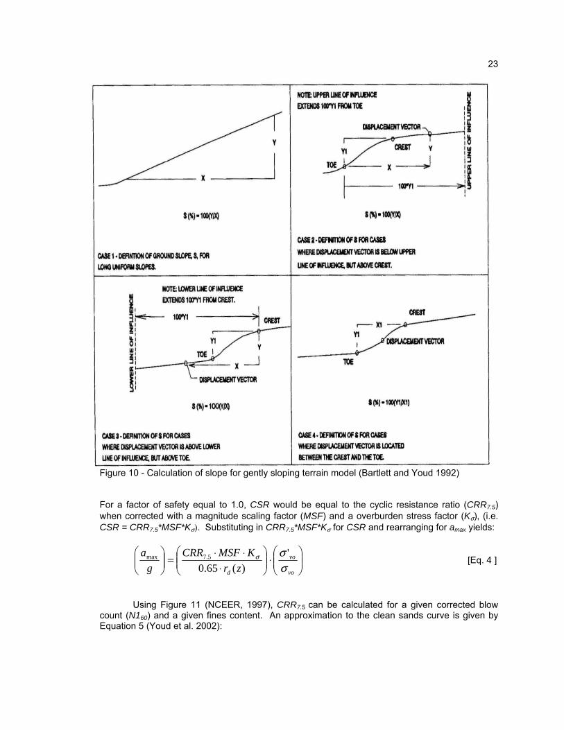
23

Figure 10 - Calculation of slope for gently sloping terrain model (Bartlett and Youd 1992) For a factor of safety equal to 1.0, CSR would be equal to the cyclic resistance ratio (CRR7.5) when corrected with a magnitude scaling factor (MSF) and a overburden stress factor (Kσ), (i.e. CSR = CRR7.5*MSF*Kσ). Substituting in CRR7.5*MSF*Kσ for CSR and rearranging for amax yields:

⎟⎟⎠

⎞⎜⎜⎝

⎛⋅⎟⎟

⎠

⎞⎜⎜⎝

⎛

⋅⋅⋅=⎟⎟

⎠

⎞⎜⎜⎝

⎛

vo

vo

d zrKMSFCRR

ga

σσσ '

)(65.05.7max [Eq. 4 ]

Using Figure 11 (NCEER, 1997), CRR7.5 can be calculated for a given corrected blow

count (N160) and a given fines content. An approximation to the clean sands curve is given by Equation 5 (Youd et al. 2002):

24

2001

]45)(10[50

135)(

)(341

2601

601

6015.7 −

+⋅+−

−=

−

−

− cs

cs

cs NN

NCRR [Eq. 5]

where the (N1)60-cs correction is done by Equation 6:

601601 )()( NN cs βα += [Eq. 6]

where α and β are coefficients determined by the fines content from equations 7 and 8 from Youd et al. (2002):

α = 0 for fines content ≤ 5% [Eq. 7a ]

α = exp[1.76-(190/FC2)] for 5% < fines content < 35% [Eq. 7b ]

α = 5.0 for fines content ≥ 35% [Eq. 7c]

β = 1.0 for fines content ≤ 5% [Eq. 8a]

β = [0.99 + (FC1.5/1000)] for 5% < fines content < 35% [Eq. 8b]

β = 1.2 for fines content ≥ 35% [Eq. 8c]

The magnitude scaling factor (MSF) accounts for the differences in a given magnitude earthquake event versus a M7.5 event because the cyclic stress ratios curves developed by Seed et al. (1985) were based on a M7.5 event. A magnitude of 7.0 was used for the study area to be consistent with the ground motion map (Wong et al. 2002) used in the study and would be a characteristic event for the Wasatch fault.

The factors recommended for the MSF from the NCEER workshop (NCEER 1997) are shown in Figure 12. The lower bound curve recommended by Idriss based upon recent research was used because it provides conservative estimates. It can be approximated by Equation 9 where Mw is the earthquake magnitude:

56.224.210

wMMSF = [ Eq. 9]

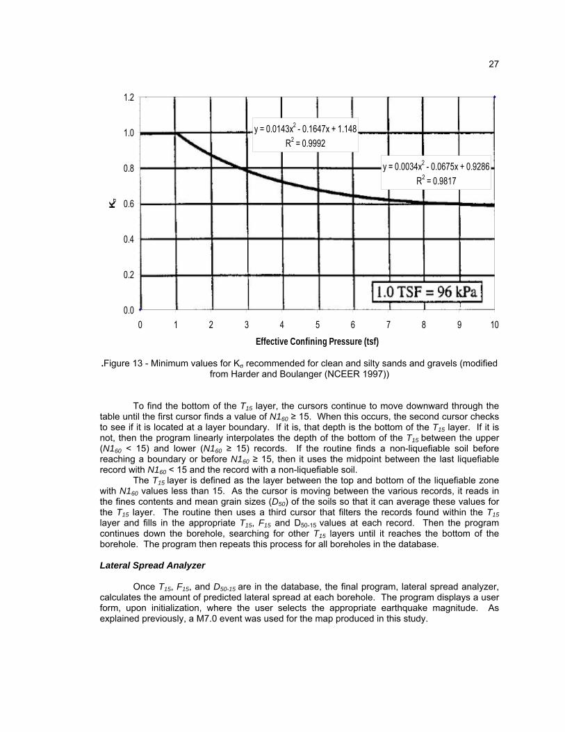
The factor Kσ accounts for the decrease in resistance that occurs from an increase in overburden (normal) stresses. New factors of Kσ have been developed (Youd and Idriss et al., 2002), but were not used because they require an estimate of relative density, which could not be calculated from the data. However, the Harder and Boulanger (NCEER 1997) curve (shown in Figure 13) can be considered an average of those curves. This is calculated from Equation 10 approximating the curve shown in Figure 13:

Kσ = 1 for σ’v ≤ 1 [Eq. 10a] Kσ = 0.0143 σ’v 2 - 0.1647 σ’v + 1.1480 for 1 < σ’v < 5 [Eq. 10b] Kσ = 0.0034 σ’v 2 - 0.0675 σ’v + 0.9286 for σ’v ≥5 [Eq. 10c]

The stress reduction coefficient (rd(z)) takes into account the flexibility of the soil profile (i.e. non-rigid behavior). The program calculates rd(z) using a regression equation approximating the mean curve plotted on Figure 14 obtained from NCEER (1997). Equation 11 inputs the depth in meters (z) of the sample being analyzed:

25

)001210.0006205.005729.04177.0000.1()001753.004052.04113.0000.1()( 25.15.0

5.15.0

zzzzzzzzrd +−+−

++−= [Eq. 11]

The total (σv) and effective vertical stresses (σ’v) were previously calculated using the

stress calculator routine, so the program just reads in these values from the BLOWFILL table. Solving Equation 4 with the values calculated in Equations 5, 9, 10, and 11 and the total and effective vertical stress values produces an estimate of the acceleration required to trigger liquefaction. The routine then compares this with the pga found by the acceleration reader program.

Figure 11 - SPT clean-sand based curve for magnitude 7.5 earthquakes with data from liquefaction case histories (NCEER 1997, Figure 2 (Modified from Seed et al. 1985))

26

Figure 12 - Magnitude Scaling Factors derived by various investigators (from NCEER 1997)

For this study, it was discovered that almost all sand samples that did not liquefy during a magnitude 7.0 event were within 0.05 g of the triggering acceleration. Because these soils were so close to triggering liquefaction, a value of 0.05 g was added to the pga to allow these soils to also liquefy. If the expected acceleration is greater than or equal to that required to initiate liquefaction, then the LIQTRIG field is given a value of “1” to indicate that liquefaction was triggered. If it is less, then the LIQTRIG field is given a value of “0” to indicate that the earthquake would not be strong enough to initiate liquefaction, and hence is incapable of producing lateral spread. In the case where insufficient data is available for the analysis, the program returns a value of “9”, so the user should examine those records and adjust them, as necessary, before continuing with the other routines.

Layer Merger (15calc)

The layer merger program finds the layers susceptible to lateral spread at each borehole and calculates the thickness (T15), the average fines content (F15), and the average mean grain size (D50-15) of the layers. At each borehole, it filters the BLOWFILL table so that it only uses the records associated with that borehole. It uses two searching cursors that cycle through every row in the BLOWFILL table in order of increasing depth. The first cursor searches for the first N160 less than 15, because soils with higher values are too dense to produce significant lateral spread (Bartlett and Youd, 1992). The second cursor always remains one row behind it. When a N160 less than 15 in a non-liquefiable sample is found by the first cursor, the second cursor looks at its record. If this record is a layer boundary, then the corresponding depth is defined as the top of the T15 layer. If it is not, then the boundary depth to the top of the T15 layer is linearly interpolated between the upper record (N160 ≥ 15) and the lower record (N160 < 15).

27

y = 0.0143x2 - 0.1647x + 1.148R2 = 0.9992

y = 0.0034x2 - 0.0675x + 0.9286R2 = 0.9817

0.0

0.2

0.4

0.6

0.8

1.0

1.2

0 1 2 3 4 5 6 7 8 9 10Effective Confining Pressure (tsf)

σ

.Figure 13 - Minimum values for Kσ recommended for clean and silty sands and gravels (modified from Harder and Boulanger (NCEER 1997))

To find the bottom of the T15 layer, the cursors continue to move downward through the table until the first cursor finds a value of N160 ≥ 15. When this occurs, the second cursor checks to see if it is located at a layer boundary. If it is, that depth is the bottom of the T15 layer. If it is not, then the program linearly interpolates the depth of the bottom of the T15 between the upper (N160 < 15) and lower (N160 ≥ 15) records. If the routine finds a non-liquefiable soil before reaching a boundary or before N160 ≥ 15, then it uses the midpoint between the last liquefiable record with N160 < 15 and the record with a non-liquefiable soil.

The T15 layer is defined as the layer between the top and bottom of the liquefiable zone with N160 values less than 15. As the cursor is moving between the various records, it reads in the fines contents and mean grain sizes (D50) of the soils so that it can average these values for the T15 layer. The routine then uses a third cursor that filters the records found within the T15 layer and fills in the appropriate T15, F15 and D50-15 values at each record. Then the program continues down the borehole, searching for other T15 layers until it reaches the bottom of the borehole. The program then repeats this process for all boreholes in the database.

Lateral Spread Analyzer

Once T15, F15, and D50-15 are in the database, the final program, lateral spread analyzer, calculates the amount of predicted lateral spread at each borehole. The program displays a user form, upon initialization, where the user selects the appropriate earthquake magnitude. As explained previously, a M7.0 event was used for the map produced in this study.

28

Figure 14 - rd versus depth curves developed by Seed and Idriss (1971) with added mean value lines approximated by Equation 11 (NCEER 1997)

To predict the lateral spread, the program cycles through each site in the SITE feature

class and filters the BLOWFILL table appropriately. To operate efficiently, as it accesses each site, it examines the groundwater depth. Sites with a groundwater depth greater than 15 m, are assigned a value of lateral spread of zero because lateral spread typically only occurs in the upper 15 m of a soil profile (Bartlett and Youd 1992). The program does not consider the borehole further and moves on to the next borehole. If the groundwater table is above 15 m for the borehole, the program cycles through each record in the BLOWFILL table below the groundwater table with a N160 less than 15 and inputs the necessary variables (W, S, T15, F15, and D50-15) to calculate the predicted lateral spread from the lateral spread regression equations developed by Bartlett and Youd (1992) with the updated regression coefficients from Youd et al. (2001). It should be recognized that the predicted lateral spread is a total displacement and not a differential displacement. Also, 90% of the predicted results are within a factor of 2 of the measured results for this model based on its dataset.

These regression equations use two models to predict the amount of lateral spread (i.e. ground slope and free face models). The program calculates the total horizontal displacement (m) based on both equations. It keeps track of the largest displacement for the borehole via an if-statement. When it reaches the end of the borehole or 15 m below the ground surface, it returns the largest predicted displacement and that value is stored in the DH field of the SITE database as the predicted lateral displacement for the borehole.

The free face model is shown in Figure 9. This type of lateral spreading occurs where there is a channel, such as that created by a stream, river or canal, which contributes to lateral spreading. Because the horizontal stress at the free face is essentially zero, the soil may slide into the channel, if the shear strength of the soil is not sufficient during the seismic event. Equation 12 predicts the amount of lateral spread for the free face condition:

Log DH = -16.713 + 1.532M – 1.406 log R* - 0.012R + 0.592 log W

29

+ 0.540 log T15 + 3.413 log (100 - F15) – 0.795 log (D50-15 + 0.1 mm) [Eq. 12] where: DH is the amount of lateral spread predicted in meters,

M is the magnitude of earthquake anticipated, R* is a function of the horizontal distance to the fault given by:

R* = R0 + R [Eq. 13]

where: R0 = 10(0.89*M – 5.64) [Eq. 14]

R is the horizontal distance to the fault (km), W is the free face ratio (%) of the height (H) and the distance (L) to the channel, T15 is the thickness (m) of the spreadable layer with N160 less than 15, F15 is the average fine contents (%) of the spreadable layer, and

D50-15 is the average mean grain size (D50) in the layer (mm).

For gently sloping ground conditions, Equation 15 predicts the amount of lateral spreading. For most cases, the ground in the study area can be considered fairly flat with nearby hills that are not considered a free-face. The following ground slope model is then applied:

Log DH = -16.213 + 1.532M – 1.406 log R* - 0.012R + 0.338 log S + 0.540 log T15 + 3.413 log (100 - F15) – 0.795 log (D5015 + 0.1 mm) [Eq. 15]

where all variables are described in Equation 14, except for S, which is the ground slope (in percent) at a site. It is not strictly a local slope and can be influenced by a nearby hill or undulating terrain, as discussed in the slope finder routine and shown in Figure 10.

Phase 3: Analysis and Map Creation

After all routines and steps are completed, these results should be verified for accuracy. Sites located very close to the fault can predict abnormally high values of lateral spread because as R becomes very small, the predicted lateral spread becomes quite large. For accurate results, it should be verified that the data lie within the limits of the models used.

As shown in Figure 15, the boreholes were color-coded based on the lateral spread hazard. Displacement intervals were chosen to correspond well with the design charts of the international building code (IBC) and building performance during lateral spreading from past earthquakes. A dark green dot indicates essentially no displacement. These should be carefully examined, as sometimes they do not predict lateral spreading because the T15 layers were missed during the sampling. The lighter green dots represent boreholes where the predicted lateral displacement is between 0 to 0.1 m (4 inches), which might cause very-slight to slight building damage that probably can be easily repaired. The yellow dots represent sites which have expected displacements between 0.1 and 0.3 m (4 inches to 12 inches), which would cause moderate to heavy damage to buildings. Sites with lateral spreading between 0.3 and 1 m (1 ft to 3 ft) are coded in orange. These locations potentially have a high hazard with severe damage to buildings expected. Sites in red have a very high hazard with more than 1 m (3 ft) of lateral spread possible. These sites may require extensive mitigation to avoid severe damage.

30

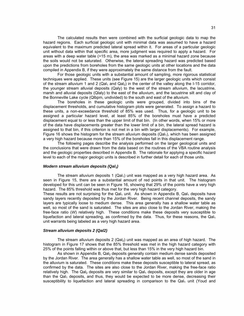
31

The calculated results then were combined with the surficial geologic data to map the hazard regions. Each surficial geologic unit with minimal data was assumed to have a hazard equivalent to the maximum predicted lateral spread within it. For areas of a particular geologic unit without data within that specific area, more judgment was required to apply a hazard. For areas with a deep water table (>15 m), the area was marked as a minimal hazard zone because the soils would not be saturated. Otherwise, the lateral spreading hazard was predicted based upon the predictions from boreholes from the same geologic units at other locations and the data compiled in Appendix B, if they were approximately the same distance from the fault.

For those geologic units with a substantial amount of sampling, more rigorous statistical techniques were applied. These units (see Figure 15) are the larger geologic units which consist of the stream alluvium 1 and 2 (Qal1 and Qal2) in the center of the valley along the I-15 corridor, the younger stream alluvial deposits (Qaly) to the west of the stream alluvium, the lacustrine, marsh and alluvial deposits (Qlaly) to the east of the alluvium, and the lacustrine silt and clay of the Bonneville Lake cycle (Qlbpm, undivided) to the south and east of the alluvium.

The boreholes in these geologic units were grouped, divided into bins of the displacement thresholds, and cumulative histogram plots were generated. To assign a hazard to these units, a non-exceedance threshold of 85% was used. Thus, for a geologic unit to be assigned a particular hazard level, at least 85% of the boreholes must have a predicted displacement equal to or less than the upper limit of that bin. (In other words, when 15% or more of the data have displacements greater than the lower limit of a bin, the lateral spread hazard is assigned to that bin, if this criterion is not met in a bin with larger displacements). For example, Figure 16 shows the histogram for the stream alluvium deposits (Qal1), which has been assigned a very high hazard because more than 15% of the boreholes fall in this displacement range.

The following pages describe the analysis performed on the larger geological units and the conclusions that were drawn from the data based on the routines of the VBA routine analysis and the geologic properties described in Appendix B. The rationale for applying a specific hazard level to each of the major geologic units is described in further detail for each of those units.

Modern stream alluvium deposits (Qal1)

The stream alluvium deposits 1 (Qal1) unit was mapped as a very high hazard area. As seen in Figure 15, there are a substantial amount of red points in that unit. The histogram developed for this unit can be seen in Figure 16, showing that 29% of the points have a very high hazard. The 85% threshold was thus met for the very high hazard category. These results are not surprising for the Qal1 unit. As shown in Appendix B, Qal1 deposits have sandy layers recently deposited by the Jordan River. Being recent channel deposits, the sandy layers are typically loose to medium dense. This area generally has a shallow water table as well, so most of the sand is saturated. The sites are also close to the Jordan River, making the free-face ratio (W) relatively high. These conditions make these deposits very susceptible to liquefaction and lateral spreading, as confirmed by the data. Thus, for these reasons, the Qal1 unit warrants being labeled as a very high hazard area. Stream alluvium deposits 2 (Qal2)

The stream alluvium deposits 2 (Qal2) unit was mapped as an area of high hazard. The histogram in Figure 17 shows that the 85% threshold was met in the high hazard category with 25% of the points falling within or above that, but less than 15% in the very high hazard bin.

As shown in Appendix B, Qal2 deposits generally contain medium dense sands deposited by the Jordan River. The area generally has a shallow water table as well, so most of the sand in the alluvium is saturated. These conditions make these deposits susceptible to lateral spread, as confirmed by the data. The sites are also close to the Jordan River, making the free-face ratio relatively high. The Qal2 deposits are very similar to Qal1 deposits, except they are older in age than the Qal1 deposits, and thus, they would be expected to be more dense, decreasing their susceptibility to liquefaction and lateral spreading in comparison to the Qal1 unit (Youd and

32

Perkins 1978). However, they still generally are susceptible to liquefaction and lateral spreading, thus a high hazard was mapped in these regions.

Figure 16 – Cumulative histogram of predicted lateral spread displacement within the Qal1 unit

.

Figure 17 – Cumulative histogram of predicted lateral spread displacement within the Qal2 unit

33

Younger stream alluvial deposits, undivided (Qaly) The younger stream alluvial deposits (Qaly) were mapped with a high hazard as well. The histogram can be seen in Figure 18. These deposits are very similar to the Qal1 and Qal2 deposits, except they can be older in age than the Qal1, and thus are generally denser, and slightly less susceptible to liquefaction hazards (Youd and Perkins 1978).

As shown in Appendix B, Qaly deposits generally can contain layers of medium dense sands deposited by the Jordan River. The area generally has a shallow water table as well, so most of the sand in the alluvium is saturated. The sites are also close to the Jordan River, making the free-face ratio somewhat high. These conditions make these deposits susceptible to liquefaction and lateral spreading, as confirmed by the data. However, these deposits are further from the Wasatch fault, and thus, R for the lateral spreading regression equation was greater, predicting less lateral spread displacement. Thus, they are not as high of a hazard as the Qal1 deposits, but they generally are still susceptible to liquefaction effects, and were mapped as such.

Figure 18 – Cumulative histogram of predicted lateral spread displacement within the Qaly unit

Lacustrine silt and clay of the Bonneville Lake cycle, undivided (Qlbpm)

The lacustrine silt and clay of the Bonneville Lake cycle (Qlbpm) unit to the east of the Qal1 at the south end of the study area were assigned a high hazard as well. The histogram shown in Figure 19 is for the Qlbpm unit located in the center of the valley only. It does not include borings from the eastern or western areas mapped as Qlbpm because geography plays a large role in the hazard in these areas. As shown in Appendix B, these deposits consist of clays with silt and sand interbeds deposited in various stages of the Lake Bonneville cycles. These deposits, as expected, are less susceptible to liquefaction than the alluvium deposits because of a much lower sand content. This particular area, however, received a high hazard because of its

34

proximity to the fault and the high ground water table, making the sand and silt interbed layers within it susceptible to liquefaction. Although very close to the fault, the Qlbpm areas further east would not be liquefiable because of the deep groundwater table. Further west, the Qlbpm areas received a low hazard because the boreholes within those areas predicted low lateral spread displacements because of greater distance to the fault.

Figure 19 – Cumulative histogram of predicted lateral spread displacement within the Qlbpm unit Young lacustrine, marsh, and alluvial deposits (Qlaly)

The young lacustrine, marsh and alluvial deposits (Qlaly) to the east of the Qal1 were assigned a high hazard. As explained in Appendix B, these recent deposits are generally loose and consist of a wide variety of poorly sorted clay, silt, and minor sand deposits from fluctuations of the Great Salt Lake. The area has a high water table, making the deposits highly susceptible to liquefaction. However, these deposits do not contain as much sand as the alluvium units. Because these deposits are thin, some of the liquefaction hazard would be controlled by the underlying geologic unit (Qlbpm) which consists of mostly silts and clays. Thus, in this area, the soil would be expected to be less susceptible to lateral spreading than the alluvium deposits.

The Qlaly unit was divided into a small northern portion and a southern portion because the northern portion had a substantial amount of very high hazard data points. The histogram in Figure 20 shows the high concentration of boreholes predicting more than a meter of displacement. Because the Qlaly unit is generally very thin, the underlying geologic units partially control the hazard in the area, and thus a complete mapping based solely on the surficial geologic units cannot be done in this area. At the northern end, the alluvial fan, Qafy, from the City Creek, deposited abundant sand as it entered the Great Salt Lake. This probably contributed to the extreme hazard found in the analysis for the borings in the northern area. On the southern end, as shown in Figure 21, the borings tended to produce less of a hazard because the underlying geologic unit was the Qlbpm unit, which has more clay and less sand, and thus would

35

be expected to have less of a hazard, as previously discussed. While there could be the similar phenomenon occurring from Parley’s Canyon, the data does not appear to have as high of a proportion of extreme hazard predictions in that area. However, there is not as much data in that region, so it is more difficult to differentiate.

Young lacustrine deposits on the west side (Qlaly and Qly) The west side of the valley mainly consists of deposits of Qlaly and Qly with a large fill area at the Kennecott tailings pond. These deposits are very similar in nature and were analyzed together because it was not feasible to separate them out. The Qly unit, however, typically would

Figure 20 – Cumulative histogram of predicted lateral spread displacement within the northern portion of the Qlaly unit contain less sand and more clay than the Qlaly unit. This was considered in the mapping of lower hazard areas close to the Great Salt Lake where the Qly deposits become more predominant.

Because these units cover such a large area, geography and proximity to the fault are contributing factors. The distance to the fault seems to influence the hazard in this area. However, if one were to analyze the potential for rupture of the Taylorsville and Granger faults, this would produce a lower magnitude earthquake, but increased lateral spreading would be predicted in the area because the seismic source is closer. However, the study by Wong et al. (2002) did not include the effects of these faults, so this study assumes that those faults do not rupture. The Qlaly and Qly deposits in the eastern part of the mapped area located adjacent to the alluvium were assigned a high hazard. These areas were divided because of the increased number of borings predicting high lateral spread hazard. There are a few explanations for this. Adjacent to the alluvium there may be some mixing of the lacustrine deposits with the alluvium deposits. The lacustrine deposits are more varied in their percentage of sand, and these areas contained a higher percentage of sand. Also, these areas are closer to the fault, and thus would

36

experience higher accelerations and larger displacements. However, there was not a sufficient amount of borings to create an accurate histogram for this area.

Figure 21 – Cumulative histogram of predicted lateral spread displacement within the southern portion of the Qlaly unit

Further west, the lateral spread hazard decreases because of the greater distance from the fault, reducing the predicted displacement. The histogram for this region can be seen in Figure 22. Although there are many borings predicting low hazard, there were a significant amount of borings (29%) predicting a moderate amount of displacement. Thus, the 85% threshold was reached within the moderate category. In analyzing the borings to the north on the west side of the Salt Lake Valley, it was found these borings had less displacement than those to the south. These northern borings were found to have less sand and more clay as the Qly deposits becomes more pronounced and become thicker. For this reason, the Qly units near the Great Salt Lake were given a low hazard.

RESULTS AND DISCUSSION

The lateral spread hazard map in Figure 23 shows the potential hazard from a rupture of the Salt Lake City and Warm Springs segments of the Wasatch Fault for a M7.0 event. It does not account for the rupture of the Taylorsville or Granger Faults on the west side of the valley. Those events would produce a different outcome.

The map offers more detail over the previous liquefaction hazard maps. For example, Anderson et al. (1994b) mapped much of the Salt Lake Valley as a high hazard area. These maps have reduced those areas to better define the hazard in the valley. In addition, the methods herein allow for the quantification of the expected displacement (i.e. liquefaction-induced ground failure) in the mapped area; whereas, with the Anderson et al. (1994b) maps, only the liquefaction potential of the deposits was mapped.

The thresholds and color coding are the same as that discussed previously. In addition, special study zones, colored in blue, were delineated in the maps to represent areas of

37

prehistoric lateral spread. Personius and Scott (1992) mapped those areas as deposits from previous lateral spreading (Qmls). Thus, they are areas of great interest for special investigations for further liquefaction and lateral spread research and are treated as such on the map.

The lateral spread hazard map shown in Figure 23 is plotted at a 1:200,000 scale. It is plotted using the Universal Transverse Mercator (UTM) Zone 12 North coordinate system based on the 1983 North American Datum (NAD83). The final map will be published by the UGS at a 1:50,000 scale as a miscellaneous publication.

Figure 22 – Cumulative histogram of predicted lateral spreading for the south-western portion of the lacustrine deposits (Qlaly and Qly) on the west side

FUTURE MAPPING EFFORTS

This section discusses the methods that will be used in developing probabilistic liquefaction triggering and probabilistic lateral spread maps in future years. This study developed a lateral spread hazard map for a scenario M7.0 earthquake to perform a check on the functionality of the developed routines and the quality of the subsurface dataset. Another part of this project assigned to the University of Utah (U of U) was to develop methods to perform probabilistic liquefaction triggering maps using the seismic input from the National Strong Motion Hazard Maps (Frankel et al. 1996). The ArcGIS® VBA programming of these methods is currently being done by Utah State University (USU). However, USU did not complete the results in time to incorporate the probabilistic triggering map for northern Salt Lake Valley in this report. The triggering routines, written by USU, and the lateral spread routines, written by the U of U will be used by the Utah Liquefaction Advisory Group (ULAG) to complete probabilistic and scenario maps for Salt Lake, Davis, Weber, Utah and Cache Counties.

38

39

Probabilistic hazard maps offer several advantages over deterministic maps. For example, probabilistic methods account for uncertainties in the subsurface data and liquefaction triggering models. Also, when coupled with probabilistic seismic hazard analyses, probabilistic methods account for a wide variety of potential earthquakes with different locations, sizes, and recurrence intervals. These methods are useful to risk assessors and planners who want to calculate the risk posed to infrastructure and other facilities by determining the mean annual risk of liquefaction and lateral spread.

The probabilistic liquefaction triggering analyses are more complex than required for a deterministic scenario map. Ostadan et al. (1991) and Marrone et al. (2003) developed methods for calculating the annual probability of liquefaction. For each N160 value an annual probability of liquefaction occurring from a seismic event of magnitude M which causes a peak ground acceleration of A at the site is given by:

],[],|[][ MAPMALPLP EE ⋅= [Eq. 16] where: PE [L] = annual probability of liquefaction during an event with a peak ground

acceleration (A) and earthquake magnitude (M), P [ L | A,M] = conditional probability of liquefaction given the peak ground acceleration (A) and the earthquake magnitude (M), and PE [A, M] = annual probability of peak ground acceleration (A) at the site due to an earthquake of magnitude (M).

This equation expresses the annual probability of liquefaction for a scenario event in a soil of given penetration resistance for a given earthquake and peak ground acceleration. The conditional probability P [L | A, M] is obtained by applying the probabilistic liquefaction potential curves developed by Seed et al. (2001). This method is similar to the deterministic liquefaction triggering methods of NCEER (1997), where probability of liquefaction curves are plotted as a function of the cyclic stress ratio induced by the earthquake and the soil’s penetration resistance (i.e., N160 values) and fines content for a M7.5 earthquake.

The cyclic stress ratio induced by the earthquake is a function of peak ground acceleration (pga), the ratio of the total vertical and effective vertical stresses, and a stress reduction factor, rd, which accounts for the flexible behavior of the soil column, when compared to rigid behavior. Also, like the deterministic method, a magnitude-scaling factor (MSF) adjusts the cyclic stress ratio induced by the earthquake to other earthquake magnitude values. Also, a correction is applied for the effective vertical stress (Kσ).

The joint probability density function P[A, M] is calculated as part of a seismic hazard analysis, or can be estimated from a seismic hazard curve, when the raw hazard calculations are not available. For example, a seismic hazard curve plots the mean annual rate of exceedance as a function of peak ground acceleration (See Figure 24). These exceedance probabilities are for all earthquake magnitude and source distance pairs in the mapped region that contribute to the level of pga plotted on the hazard curve. Also, because the hazard curve is a cumulative probability distribution function, it must be converted to a probability density function by differencing or differentiating the hazard curve. Lastly, because liquefaction and lateral spread analyses require an estimate of the M associated with the specific values of A from the hazard curve, often the mean or median M for each A value is used to represent the M in the liquefaction and lateral spread calculations. Mean and median estimates of M for all of the potential earthquakes contributing to the exceedance probability of A can be obtained from the National Seismic Hazard Map website (http://eqhazmaps.usgs.gov/) from the deaggregation plots and output.

40

However, because the USGS web published values are given for a relatively course grid and the deaggregations are only available for select points on the hazard curve, ULAG chose to obtain the P[A, M] directly from the USGS at a finer grid spacing of 0.025 degrees. The requested

Figure 24 – Sample seismic hazard curve hazard curve contained several values of A (0.01, 0.05, 0.1, 0.2, 0.3, 0.4, 0.5, 0.6, 0.7, 0.8, 0.9 and 1.0 g) to obtain a relatively uniform spacing of the hazard curve. For each value of A, the USGS provided a separate file with the exceedance probabilities of A, modal M, R (km) and the gridded locations.

The probability that pga is between two values of A can be found by differencing the values of exceedance probabilities. This difference, the “interval probability,” is the probability that A is found within that bin. The A value corresponding to the mid point of each bin is calculated and the interval probability is used as a point estimate of the P[A] for the mid point of A.The final aggregation of the liquefaction hazard can then be computed from:

)](,[)](,|[][ ii

iii AMAPAMALPLP ∑ ⋅= [Eq. 17]

where: P[L] = annual probability of liquefaction,

P [ L | Ai, M(Ai)] = conditional probability of liquefaction given the peak ground

acceleration (Ai) and the earthquake magnitude (M(Ai)) for that acceleration,

P [Ai, M(Ai)] = annual probability of peak ground acceleration and earthquake

magnitude for that acceleration, and

41

M(Ai) = the weighted modal magnitude of the earthquakes contributing to the

annual probability of Ai.

Note that for this equation, the interval probability and its associated mid point value of Ai are substituted for P[Ai, M(Ai)]. The aggregated probability from Equation 17 is the probability that will be used to estimate the liquefaction potential for the probabilistic liquefaction triggering maps. As previously discussed, these maps will provide estimates of those areas prone to liquefaction and the mean annual hazard of liquefaction of these areas.

A probabilistic lateral spread map will be developed in a similar manner. The probability of lateral spread exceeding a threshold value P[DH > x] is computed for each borehole for given values of Ai with corresponding values of M and R (See Figure 25). This probability of exceedance is calculated from the standard error of the regression model for given values of M, R, and A. The Bartlett-Youd regression equation (Youd et al. 2002) will be used to estimate DH and the exceedance probabilities using: P[ (DH>x) | Ai, M(Ai), R(Ai)] = 1 – Fz(z) [Eq. 18]

where: DH = the predicted lateral spread displacement for A, M, and R, x = a threshold value = 0.1, 03, or 1 m, as explained below,

R(Ai) = the horizontal distance from the earthquake to the site being evaluated, as defined in Bartlett and Youd (1992), as a function of Ai,

Fz(z) = the cumulative density function (CDF) for the standard normal variate, z,

as taken from a CDF table of the standard normal distribution found in a general statistics text. (This can also be found in Table C-1, Kramer 1996, p. 593)

where z is computed by:

)log(

)log()log(

HD

HH xDDzσ

=−= [Eq. 19]

where: log(DH) = the log of the computed displacement by the Youd et al. (2002)

equations,

log(DH = x) = the log of the desired threshold displacement, x = 0.1, 0.3, and 1 m, as discussed below, and

σlog(DH) = the standard error of the Youd et al. (2002) regression equations.

The lateral spread probability calculator program in Appendix C performs the calculations of the exceedance probability of lateral spread exceeding the threshold. The threshold values for which the probabilistic lateral spread maps will be computed are 0.1, 0.3 and 1.0 m. These are the same threshold values that were used in the deterministic lateral spread map of this report. To complete the probabilistic calculations, the probability chain is calculated and aggregated using Equation 20:

42

Figure 25 – Schematic illustration of conditional probability of DH exceeding a threshold of x for a given magnitude, distance, and acceleration (modified from Kramer 1996, p. 127)

)](),(,[)](),(,|[]|[][ iiii

iiiHH ARAMAPARAMALPLxDPxDP ∑ ⋅⋅>=> [Eq. 20]

This probability represents the probability that DH exceeds a given threshold value for the

summation of the values of Ai, the M and R pair associated with Ai, and the subsurface conditions given in the borehole. Aggregating (i.e. summing) for all A values on the seismic hazard curve produces the mean annual exceedance probability of DH. These probabilities will then be evaluated to produce hazard maps in a manner similar to that done in this study. These hazard maps will be produced in future years by ULAG for use by various government and private agencies. It is hoped that these maps will be implemented in practice to more fully describe the seismic hazard at a site than can be obtained with deterministic or scenario maps. Further, even though these methods are being applied to a regional map, they are also valid for calculating the liquefaction and lateral spread hazard at a given site. Lastly, this study has provided an ArcGIS® database for geotechnical data in the Salt Lake Valley. It is hoped that these beginnings will inspire other researches and agencies to contribute to this data gathering effort. Such contributions will greatly improve the knowledge of subsurface conditions and their variability in the mapped areas.

log R r

P[DH>x | Ai, M(Ai), R(Ai)]

M = m

x

DH

43

APPENDIX A

DATABASE STRUCTURE

44 Table 2 - Database structure for the SITE table Field Name Type Description OBJECTIDNO AutoNumber This is a field for ArcGIS- DO NOT EDIT THIS FIELD. SITEIDNO Integer Site identification number RENUMBERED Yes/No Used for renumbering site id REPORT Text Name of Report for Borehole Data REFERENCE Text Name and Date of Authors SITENAME Text Name of Site BORING Text Boring Name PAGENO Text Pg. No. in report of Boring log BOREELEV Double Surface Elevation of Borehole (m)

ELEVEST Single Quality of Elevation Estimate: 1 = documented, 2 = reasonably estimated, 3 = guess from other source

BORINGDEPTH Double The total depth of the borehole DATE_ Date/Time Date of Boring LOCATION Text Street Address NORTHING Double Northing Coordinate (UTM NAD83 Z12N) EASTING Double Easting Coordinate (UTM NAD83 Z12N) LATITUDE Double Latitude of Boring LONGITUDE Double Longitude of Boring

LATITEST Text Quality of Lat & Long Est: 1 = documented, 2 = reasonably estimated, 3 = guess from other source

GWDATE Date/Time Date of Groundwater

GWEST Long Integer Quality of Depth to Groundwater

DEPTHGW Double Depth to Groundwater (ft) DRILLCONT Text The Contractor doing the drilling LOGGER Text The name of the person logging the boring RIGTYPE Text Name or Type of Drill Rig DRILLMETH Text Method used for drilling

BoreDiam Double Diameter of the Borehole (in) for calculating corrected Blow Counts (CB)

BoreDiamEst Integer Quality of the Estimate 1= documented, 2= reasonably estimated, 3= guess from other source

BIT_ Text Type of Bit used DRILLER Text Name of Driller HAMMER_TYPE Text Type of SPT Hammer

HAMMER_MASS Double The hammer mass used to drive the split-spoon sampler. The standard mass is 140 lb (63.5 kg)

HAMMER_ RELEASE Text The mechanism used to lift and drop the hammer.

HAMMER_DROP_HEIGHT

Long Integer The hammer drop height for SPT Penetration.

ENERGY Integer [HAM_ER] Hammer Energy Ratio (%)

45 Table 2 - Database structure for the SITE table (Continued)

HAMEST Text Quality of Hammer Est: 1 = documented, 2 = reasonably estimated, 3 = guess from other source

ROD_TYPE Text Type of Drilling Rod ROD_ EXTERNAL

Long Integer The external diameter of the sampling rods.

ROD_WEIGHT Long Integer The drive rod weight per unit length.

CATHEAD_DIAMETER

Long Integer

The diameter of the cathead used to pull the rope attached to the hammer. Typical diameters range from 6 to 10 inches (150 to 250 mm)

ROPE_TURNS Long Integer

The number of rope turns on the cathead for performing the SPT. Max allowed Number of turns is 2 1/4.

RODTYPEEST Text Quality of Rod Doc: 1 = documented, 2 = reasonably estimated, 3 = guess from other source

Local Slope Double The local slope at the site (Calculated using ArcGIS Spatial Analyst). Filled in by the Slopefinder Routine.

SLOPE Double The slope according to the Bartlett/Youd Lateral Spread Regression Definition. Filled in by the Slopefinder Routine.

GEOLUNIT Text The Surficial Geological Unit that the SITE is located in

VS12 Double The 12 m (40ft) Shear Wave Velocity Measurement (filled in by VSFinder). Used to calculate rd.

VS30 Double The 30m Shear Wave Velocity Measurement (filled in by VSFinder). Used to classify the SITE according to IBC

VSEST Integer The quality of the VS measurement 1= test done in the borehole, 2= test done nearby in the same geological unit, 3= guess from other source

WFreeFace Double The Free Face Ratio (H/L*100%). Filled in by the Wfinder Routine.

R Double The horizontal distance to the fault (R, km). Filled in by the RFinder Routine.

EARTHQUAKE Text Earthquake Used in Analysis MAGNITUDE Double Magnitude of Earthquake

acc Double The estimated peak ground acceleration at the site (g). Filled in by the Acceleration Reader Routine

accEst Integer The quality of the Estimate of the acceleration

DH Double The maximum predicted lateral spreading in the borehole. Filled in by the Lateral Spread Calculator Routine.

NOTES Memo This is a memo field for any additional notes that need to be attached to the record.

PDF Memo This is a hyperlink to the pdf file where a scanned image of the log can be found

Shape OLE Object This is a field for ArcGIS- DO NOT EDIT THIS FIELD.

46 Table 3 - Database structure for the BLOW and BLOWFILL tables

Name Type Description

OBJECTID AutoNumber This field is used by ArcGIS as a unique identifier for each record

SITEIDNO Integer Site identification number BOREIDNO Text Same as BORING in site.dbf RENUMBERED Yes/No Used for renumbering site ID DEPTH Double Depth of Sample (ft) DEPTHM Double Depth of Sample (m) BOUNDARY Yes/No If recorded layer is boundary. T=layer boundary ELEV Double Elevation of sample (ft) do not fill in this field ELEVM Double Elevation of sample (m) do not need to fill in this field NVALUE Double [NM] SPT N value (blow/ft) BLOWS1 Long Integer Blow Count for first 6" BLOWS2 Long Integer Blow Count for second 6" BLOWS3 Long Integer Blow Count for third 6" BLOWS4 Long Integer Blow Count for fourth 6"

ESTNM Text Quality of SPT Estimate: 1 = documented, 2 = reasonably estimated, 3 = guess from other source

SAMPLER Text Type of Sampler ("Standard Split-Spoon Sampler";"Dames and Moore Sampler";"Modified California Sampler")

SAMPLEREST Integer Qualtiy of Sampler Doc: 1 = documented, 2 = reasonably estimated, 3 = guess from other source

SAMPLER_INSIDE_DIAMETER Double [SAMPLERID] Inside dia. of sampler (mm)

SAMPLER_OUTSIDE_DIAMETER Double [SAMPLEROD] Outside dia. of sampler (mm)

SAMPLERLENGTH Double The length of the split spoon sampler LINER Yes/No The use of a liner in the sampling BASKET Yes/No The use of a basket retainer NMCPT Double SPT N Estimated from CPT

CPTQUAL Long Integer Quality of CPT Data: 1 = documented, 2 = reasonably estimated, 3 = guess from other source

SOILTYPE Text Soil Type Description UCSC Text Unified Soil Classification System Label

ESTUCSC Text Quality of UCSC: 1=laboratory 2=field 3= guess from other source

AASHTO Text Aashto Classification w/ Group Index

ESTAASHTO Integer Quality of AASHTO Classification: 1=laboratory 2=field 3= guess from other source

GEOLUNIT Text Name of Geologic Unit

ESTGEOL Text Quality of Geological Estimate: 1 = mapped, 2 = guess when it is deeper, 3 = geotechnical report w/o geologist

47 Table 3 - Database structure for the BLOW and BLOWFILL tables (Continued)

DEPENV Text Depositional Environment

SITERESUN Text Site Response Unit

ESTSITERES Integer Site Response Data Qualifier: 1 = mapped, 2 = guess when it is deeper, 3 = geotechnical report without geologist

CLASS Double Do not need to fill in this field DRYUNIT Double Dry Unit Weight (kN/m^3)

ESTDRY Text Quality of DUW: 1 = documented, 2 = reasonably estimated, 3 = guess from other source

WETUNIT Double Moist Unit Weight (kN/m^3)

ESTWET Text Quality of MUW: 1 = documented, 2 = reasonably estimated, 3 = guess from other source

DRYUNITPCF Double Dry unit weight (pcf) WETUNITPCF Double Wet Unit Weight (pcf) MOISTURE_ CONTENT Double The moisture content (%) of the soil

ESTMOIST Text Quality of WC: 1 = documented, 2 = reasonably estimated, 3 = guess from other source

DENSITY Double Relative Soil Density- Do not fill out this field RELDENSITY Double Relative Soil Density: Do not fill out this field SPGRAVITY Double Specific Gravity: 2.65 sand, 2.70 silt, and 2.75 clay

ESTSPGR Text Quality of Specific Gravity: 1 = documented, 2 = reasonably estimated, 3 = guess from other source

PERGRAVEL Double Gravel Content (%) PERSAND Double Sand Content (%) FINES Double Fines Content (%) CLAY Integer Clay Content (%)

ESTFINES Text Quality of Fines Estimate: 1 = documented, 2 = reasonably estimated, 3 = guess from other source

ESTCLAY Text Quality of Clay Estimate: 1 = documented, 2 = reasonably estimated, 3 = guess from other source

NONLIQ Yes/No T= Nonliquefiable

ESTNONLIQ Text Quality of Nonliquefiable Estimate: D50 Double Mean Grain size (mm)

D50EST Text Quality of D50 Estimate: 1 = documented, 2 = reasonably estimated, 3 = guess from other source

LIQUIDLIMIT Double Liquid Limit LIQUIDLIMIT_ METHOD Text Method used for determining liquid limit

LIQUIDLIMIT_PREP Text Method used for preparing sample for liquid limit PLASTICLIMIT Double Plastic Limit PLASTICINDEX Double Plastic Index = Liquid Limit - Plastic Limit SHRINKAGELIMIT Double Shrinkage Limit LIQUIDINDEX Double The Liquid Index

48 Table 3 - Database Structure for Blow Table (Continued)

NATURALWATERCONTENT Double Natural Water Content

ESTATT Integer Data Qualifier for Atterberg Limits: 1 = documented on report, 2 = reasonably estimated from another layer on same report, 3 = guess from other source

BOTTOM Double The depth to the bottom of the current layer VS Double Shear Wave Velocity CPT Yes/No If the record is CPT data QC Double For CPT Data QCUNC Double For CPT Data SLEEVE Double For CPT Data FRATIO Double For CPT Data PPRESSURE Double For CPT Data EXCIT Double For CPT Data QCEST Text For CPT Data EXCITATION Double For CPT Data INTERP Text For CPT Data

MoistUnitWeight Double The calculated moist unit weight. From the Stress Calculator Routine.

SatUnitWeight Double The calculated saturated unit weight. From the Stress Calculator Routine.

TotalStress Double The total stress at the depth of the record. From the Stress Calculator Routine.

EffectiveStress Double The effective Stress at the depth of the record. From the Stress Calculator Routine.

CB Double The correction for the borehole diameter. From the N160 Calculator Routine.

CE Double The correction for the energy ratio. From the N160 Calculator Routine.

CN Double The overburden correction factor. From the N160 Calculator Routine.

CR Double The correction for the rod length. From the N160 Calculator Routine.

CS Double The correction for the sampler. From the N160 Calculator Routine.

N160 Double The corrected blow count for an energy of 60% and corrected for overburden. From the N160 Calculator Routine.

rd Double The reduction factor for depth. From the Atrigger Calculator Routine.

CRR Double Cyclic Resistance Ratio. From the Atrigger Calculator Routine.

N160CS Double The blow count corrected for clean sands. From the Atrigger Calculator Routine.

Ksigma Double A correction for depth. From the Atrigger Calculator. MSF Double A magnitude scaling factor. From the Atrigger Calculator.

Atrig Double The acceleration required to trigger liquefaction. From the Atrigger Calculator Routine.

49 Table 3 - Database Structure for Blow Table (Continued)

liqtrig Integer Indicates if liquefaction was triggered. (the acceleration at the site was greater than that required to trigger liquefaction). From the Atrigger Calculator Routine.

T15 Double The thickness of the spreadable layer (m). From the Layer Merger (15Calc) Routine

D5015 Double The average mean grain size D5015 for the spreadable layer. From the Layer Merger (15Calc) Routine

F15 Double The average fines content for the spreadable layer. From the Layer Merger (15Calc) Routine

zLiqTop Double The depth at the top of the liquefiable layer. From the Layer Merger (15Calc) Routine

zLiqBot Double The depth at the bottom of the liquefiable layer. From the Layer Merger (15Calc) Routine

DHS Double The gently sloping terrain model predicted value of lateral spreading (m). From the Lateral Spread Calculator Routine.

DHW Double The free face model predicted value of lateral spreading (m). From the Layer Merger (15Calc) Routine.

Comments Text A field for generic comments. Footnote Text References the Footnote table when it is needed

TESTS Text Indicates other tests done on the soil at that depth. Not Required

Recovery Double The percent of the sample that was recovered. Not Required

Lithology Integer 1= the record is just there as a soil description, but should not be used in the analysis. Not Required.

ERRORDUWorGS Integer

Indicates if an estimate of 15 kN/m3 needed to be used for the Dry Unit Weight, or if 2.7 was needed to be used for the specific gravity in the Routines. Created by the Stress Calculator routine.

APPENDIX B

GEOLOGIC UNIT DESCRIPTIONS

51

51

The descriptions of the geologic units given in this appendix are modified from

Personious and Scott (1992) and Biek et al. (2004). In addition, histograms from the dataset have been included to show the Soil-type, N160 blow-count distribution for granular soils, and Plastic Index distribution for fine soils within the major geologic units with adequate sampling. Table 4 shows the symbols used to display the units on the map. Table 4 - Geologic unit symbols and descriptions

Map Symbol Name Description Age Page

Number Stream Alluvium 70-77

Qal1 Modern stream alluvium 1 Upper Holocene 70

Qal2 Stream alluvium 2 Middle Holocene to Upper Pleistocene 72

Qaly Younger stream alluvial

deposits,undivided Holocene to Upper Pleistocene 74

Qalp

Stream alluvium related to the Provo (regressive) phase of the Bonneville lake cycle

Upper Pleistocene 76

Qalb

Alluvial deposits related to the Bonneville (transgressive) phase of the Bonneville lake cycle

Upper Pleistocene 77

Alluvial-Fan Deposits 77-81

Qaf1 Modern alluvial-fan deposits 1 Upper Holocene 77

Qaf2 Alluvial-fan deposits 2 Middle Holocene to Upper Pleistocene 78

Qafy Younger alluvial-fan deposits, undivided

Holocene to Upper Pleistocene 80

Qafp

Alluvial-fan deposits related to the Provo (regressive) phase of the Bonneville lake cycle

Upper Pleistocene 80

Qafb

Alluvial-fan deposits related to the Bonneville (transgressive) phase of the Bonneville lake cycle

Upper Pleistocene 80

52

52

Table 4 - (continued)

Alluvial Fan Deposits (continued) 77-81

Qaf4 Alluvial-fan deposits 4 Upper to Middle Pleistocene 80

Qaf5 Alluvial-fan deposits 5 Middle Pleistocene 81

Qafo Older alluvial-fan deposits, undivided

Upper to Middle Pleistocene 81

Lacustrine Deposits 81-97

Qly Young lacustrine and marsh deposits Holocene 81

Qlaly Young lacustrine, marsh, and alluvial deposits

Holocene to Upper Pleistocene 83

Qlpg

Lacustrine gravel and sand related to the Provo (regressive) phase of the Bonneville lake cycle

Upper Pleistocene 85

Qlpm Lacustrine clay and silt related to the Provo (regressive) phase of the Bonneville Lake Cycle

Upper Pleistocene 87

Qlbg

Lacustrine gravel and sand related to the Bonneville (transgressive) phase of the Bonneville lake cycle

Upper Pleistocene 87

Qlbs

Lacustrine sand and silt related to the Bonneville (transgressive) phase of the Bonneville lake cycle

Upper Pleistocene 88

Qlbm

Laucstrine clay and silt related to the Bonneville (transgressive) phase of the Bonneville lake cycle

Upper Pleistocene 90

Qlbpg Lacustrine gravel and sand of the Provo and Bonneville lake cycles, undivided

Upper Pleistocene 92

Qlbps Lacustrine sand and silt of the Provo and Bonneville lake cycles, undivided

Upper Pleistocene 94

Qlbpm Lacustrine silt and clay of the Provo and Bonneville lake cycles, undvided

Upper Pleistocene 96

53

53

Table 4 - (continued)

Mass movement deposits 98

Qmsy Younger landslide deposits Historical to Upper Pleistocene 98

Qmls Lateral-spread deposits Holocene to Upper Pleistocene 98

Qmt Talus deposits Holocene to Upper Pleistocene 98

Colluvial Deposits 99

Qchs Hillslope colluvium Holocene to Upper Pleistocene 99

Qca Colluvium and alluvium, undivided

Holocene to Middle Pleistocene 99

Eolian Deposits 99

Qes Eolian sand Holocene to upper Pleistocene 99

Artificial Deposits 99-100

Qf Artificial fill Historical 100

Bedrock 100

Tn Tertiary sedimentary and volcanic rocks Neogene 100

Tp Tertiary sedimentary and volcanic rocks Paleogene 100

Mz Mesozoic sedimentary rocks Cretaceous to Triassic 100

Pz Paleozoic sedimentary rocks Permian to Cambrian 100

pC Precambrian metamorphic rocks Proerozoic and Archean 100

54

54

Alluvial Deposits

[Consist of variable amounts of gravel, sand, silt, and minor clay, deposited by perennial and intermittent streams. Map units are separated into five deposits of stream alluvium and eight alluvial-fan deposits. Stream deposits are mapped on flood plains and as thin terrace deposits along perennial streams; gravel in these deposits is generally more rounded and better sorted than that in alluvial-fan deposits. Stream deposits are differentiated by their stratigraphic and geomorphic positions relative to glacial deposits of the Bells Canyon advance and to levels of the Bonneville lake cycle, which occupied the valley from about 32,000 to 10,000 years ago (Currey and Oviatt 1985), and modern stream level. Alluvial-fan deposits occur on the piedmont at the mouths of most canyons along the mountain front. Fan deposits are differentiated according to the following criteria: (1) their relation to lacustrine deposits and shorelines of known age; (2) their relation to modern stream level; and (3) differences in soil development. The Holocene fan deposits (Qaf1, Qaf2) are differentiated by soil properties as outlined by Shroba (1982, 1984); soil-horizon designations follow those of Birkeland (1984).]

Stream Alluvium

Qal1 – Modern stream alluvium 1 (upper Holocene). Poorly to moderately sorted sand, silt, and minor clay and gravel along the Jordan River and lower reaches of its tributaries; deposits along upper reaches of tributaries consist of pebble and cobble gravel, and minor sand and silt; parallel bedding and cross-bedding; forms modern flood plain and terraces less than 5 m above modern stream level; subject to flooding and high water table; exposed thickness 1 - 3 m.

The Qal1 unit it is composed of well–graded sand and silty sand (67%) with some silt (11%) and clay (15%), as shown in Figure 26. These deposits are medium dense, with a substantial amount of very loose and loose soils, as shown in Figure 27. Thus, these deposits are very susceptible to liquefaction and lateral spreading. As shown in Figure 28, the fine soils found within this unit are generally medium plastic.

Qal2 - Stream alluvium 2 (middle Holocene to upper Pleistocene). Poorly to

moderately sorted sand, silt, clay, and local gravel along Jordan River and lower reaches of its tributaries; deposits along upper reaches of tributaries consist of pebble and cobble gravel, and minor sand and silt; parallel bedding and cross-bedding; deposited by streams graded to recessional stands of Lake Bonneville and to lakes of early Holocene age; forms terraces more than 5 m above modern stream level, usually inset into deposits of the Bonneville lake cycle; exposed thickness 1 - 5 m.

The Qal2 is composed of well–graded sand and silty sand (66%) with some silt (12%) and clay (17%), as shown in Figure 29. These deposits are medium dense, with a substantial amount of very loose and loose deposits, as shown in Figure 30. The loose deposits, however, are less than that found in the Qal1 unit. These deposits are susceptible to liquefaction and lateral spreading. As shown in Figure 31, the fines are generally low to medium plastic fines.

Qaly- Younger stream alluvial deposits (Holocene to Upper Pleistocene). Consists

of moderately sorted sand, silt, clay, and pebble to boulder gravel deposited in stream channels and flood plains; includes abandoned flood plains that postdate the Bonneville shoreline of latest Pleistocene Lake Bonneville; the alluvial deposits are incised by active stream channels, and locally include small alluvial-fan and colluvial deposits; includes modern and older, post-Lake Bonneville stream deposits (Qal1 and Qal2) that are undifferentiated because units are complexly overlapping; mapped along streams emanating from the Oquirrh Mountains; forms terraces along Jordan River from Taylorsville north to Salt Lake City International Airport; probably less than 6 m thick.

The Qaly unit contains well–graded sand and silty sand (60%) with some silt (18%) and clay (19%), as shown in Figure 32. These deposits are medium dense, with a substantial amount of loose and medium dense deposits, as shown in Figure 33. Thus, these deposits are

55

55

susceptible to liquefaction and lateral spreading. There was insufficient data to analyze the plasticity of the fine soils within this unit.

Qalp - Stream alluvium related to the Provo (regressive) phase of the Bonneville

lake cycle (upper Pleistocene). Clast-supported pebble and cobble gravel, locally bouldery, in a matrix of sand and silt; poorly sorted, clasts subangular to round; parallel bedding and cross-bedding locally massive; deposited by streams graded to the Provo shoreline and other shorelines of the regressive phase of the Bonneville lake cycle; also deposited as topset beds on deltaic deposits related to the Provo shoreline; fluvial scarps are preserved on the surfaces of some deposits; thickness 1 - 10 m.

The Qalp unit is composed of sand (49%) and gravel (34%) with some silt, as shown in Figure 34. These deposits are very dense, as shown in Figure 35. Thus, these deposits are not very susceptible to liquefaction and lateral spreading. Since these deposits are older in age than the other alluvial deposits, this is expected (Youd-Perkins 1978). There was insufficient data to analyze the plasticity of the fine soils within this unit.

Qalb- Stream alluvium related to the Bonneville (transgressive) phase of the

Bonneville lake cycle (Upper Pleistocene). Moderately sorted sand, silt, and pebble to boulder gravel deposited by streams graded to shorelines of the transgressive phase of Lake Bonneville; incised by active streams; mapped south of Harker’s Canyon; about 6 m thick.

Alluvial-fan Deposits

Qaf1- Modern alluvial-fan deposits 1 (Upper Holocene). Poorly to moderately sorted,

weakly to non-stratified, clay- to boulder-size sediment in a matrix of sand and silty sand deposited principally by debris flows at the mouths of small, active drainages; upper parts characterized by abundant boulders and debris-flow levies that radiate away from the fan apex; equivalent to the younger part of Qafy, but differentiated where deposits can be mapped separately; may contain small deposits of Qaf2; many deposits of unit Qaf1 too small to be shown at the map scale are included in unit Qaf2; no shorelines present on surfaces; typical soil profiles range from A-Cn to A-Bw-Cox-Cn; generally less than 9 m thick.

Qaf2- Alluvial-fan deposits 2 (Middle Holocene to Upper Pleistocene). Clast-supported pebble and cobble gravel, locally bouldery, in a matrix of sand and silty sand; poorly sorted; clasts sub-angular to round; thin to thick, parallel bedding and cross-bedding; locally massive; deposited by perennial and intermittent streams, debris flows, and debris floods (hyper-concentrated floods) graded approximately to modern stream level; may contain small deposits of units Qaf1, especially near fan heads and along active stream channels; no shorelines present on surfaces; typical soil profiles range from A-Bw-Cox-Cn to A-Bt(weak)-Cox-Cn; typically 1 to >10 m thick.

The Qaf2 unit contains a substantial amount of sand (36%) and gravel (34%) with some silt (18%) and clay (12%), as shown in Figure 36. These deposits are dense, as shown in Figure 37. Thus, these deposits are not very susceptible to liquefaction and lateral spreading. As shown in Figure 38, the fines are generally of low plasticity.

Qafy- Younger alluvial-fan deposits, undivided (Holocene to Upper Pleistocene).

Postdates the regressive phase of the Bonneville lake cycle. Poorly to moderately sorted, weakly to nonstratified, clay- to boulder-size sediment deposited principally by debris flows, debris floods, and streams; commonly obscures Lake Bonneville shorelines; equivalent to modern alluvial-fan deposits (Qaf1) and older, post-Lake Bonneville alluvial-fan deposits (Qaf2) that are undifferentiated because units are complexly overlapping or too small to show separately; upper parts of fans are locally deeply incised; mapped near the Salt Lake Salient near the margins of the Oquirrh Mountains extending as much as 5 km (3 miles) from the range front where drainages incise Lake Bonneville deposits; probably less than 12 m thick.

56

56

Qafp- Alluvial-fan deposits related to the Provo (regressive) phase of the

Bonneville lake cycle (Upper Pleistocene). Poorly to moderately sorted, clay- to cobble-size sediment deposited principally by debris flows graded to the Provo shoreline; incised by active streams; underlies the broad, gently sloping floor of Little Valley above the Provo shoreline in the northwest part of the Magna quadrangle; probably less than about 12 m thick.

Qafb- Alluvial-fan deposits related to the Bonneville (transgressive) phase of the

Bonneville lake cycle (Upper Pleistocene). Poorly to moderately sorted, clay to cobble-size sediment deposited principally by debris flows graded to the Bonneville shoreline; incised by active streams; may be covered by thin deposits of posttransgressive phase alluvium and colluvium; typical soil profile, A-Bt-Cox-C; probably less than about 12 m thick.

Qaf4 - Alluvial-fan deposits 4 (Upper to Middle Pleistocene). Clast-supported pebble

and cobble gravel, locally bouldery, in a matrix of sand and silty sand; poorly sorted; clasts sub-angular to round; thin to thick, parallel bedding and cross-bedding; locally massive; forms small fans and fan remnants topographically above or cut by the Bonneville shoreline; correlative deposits probably underlie much of the map area and are buried by younger deposits downslope from the Bonneville shoreline; typical soil profile, A-Bt(moderate-strong)-Cox-Cn; usually 1 to > 10 m thick.

Qaf5 - Fan alluvium 5 (Middle Pleistocene). Clast-supported pebble and cobble gravel,

locally bouldery, in a matrix of sand and silty sand; poorly sorted; clasts subangular to round; thin to thick, parallel bedding and cross-bedding; locally massively bedded; forms high fan remnants on ridge tops near front of Wasatch Range; some remnants may be deposits of old till that lack morainal morphology; typical soil profile, A-Bt(strong)-Cox-Cn; usually 1 to >10 m thick.

Qafo- Older alluvial-fan deposits, undivided (Upper to Middle Pleistocene). Poorly

to moderately sorted, weakly to nonstratified, clay- to boulder-size sediment deposited principally by debris flows, at the base of the Oquirrh Mountains, mapped as part of the Harkers fanglomerate by Slentz (1955); mapped near the Salt Lake salient, where old fan deposits have not been differentiated; forms deeply dissected alluvial apron near Coon Canyon; exposed deposits are truncated by, and thus predate, the Bonneville shoreline; upper to middle Pleistocene age is suggested by development of stage II or III calcic paleosols on fan surfaces, characterized by calcium-carbonate coatings on clasts in a loose matrix with dispersed calcium carbonate; underlies piedmont slopes below the Bonneville shoreline beneath a thin veneer of lacustrine deposits; may be undifferentiated from underlying middle Pleistocene to late Miocene[?] alluvial-fan deposits where mapped in deeply incised stream channels; exposed thickness as much as 45 m.

Lacustrine Deposits

[Consist of gravel, sand, silt, and clay deposited in Lake Bonneville (Bonneville lake cycle), Great Salt Lake, and other smaller lakes. These deposits are divided into four groups: (1) deposits that postdate the Bonneville lake cycle; (2) deposits associated with the Provo shoreline and the regressive phase of the Bonneville lake cycle; (3) deposits associated with the Bonneville shoreline and the transgressive phase of the Bonneville lake cycle; and (4) undivided sediments of the Bonneville lake cycle deposited at altitudes below the Provo shoreline that cannot be assigned to either phase of the Bonneville lake cycle. Sediments deposited near the mountain front are mostly gravel and sand; silt and clay were deposited in quieter, deeper water on the valley (lake) bottom, in sheltered bays between headlands, and less commonly in lagoons behind barrier beaches].

57

57

Deposits Postdating the Bonneville Lake Cycle (Curry and Oviatt 1985)

Qly- Young lacustrine and marsh deposits (Holocene). Silt, clay, and minor sand deposited in shallow lakes and marshes after the regressive phase; commonly organic rich; locally may contain peat deposits; occur in areas of standing water or where the water table is or has recently been at the ground surface; includes sediments in mud flats or playas exposed by fluctuations of the Great Salt Lake; commonly grade into and may contain small deposits of unit Qlbpm; subject to lacustrine flooding and high water table; thickness < 5 m.

The Qly unit contains mostly clay (77%) with some silt (15%) and sand (8%), as shown in Figure 39. There was insufficient data to create a histogram for the blow-counts within granular soils in this unit. However, they are generally loose deposits. This combined with a high water table make the granular soils within these deposits very susceptible to liquefaction and lateral spreading. As shown in Figure 40, the fines are highly plastic fines.

Qlaly- Young lacustrine, marsh, and alluvial deposits (Holocene to upper

Pleistocene). Undivided clay, silt, sand, peat, and very minor pebble gravel; deposited after the regressive phase of the Bonneville lake cycle in shallow lakes and marshes, in deltas along the lower reaches of the Jordan River, and on distal parts of alluvial fans; deposited in mud flats or playas exposed by fluctuations of Great Salt Lake; local accumulations of gypsum, halite, and other salts commonly form a thin crust on the ground surface; unit probably contains small deposits of unit Qmls in urbanized areas; thickness 1 to > 3 m.

The Qlaly unit is composed of mostly clay (51%) and sand (29%) with a substantial amount of silts (18%) as shown in Figure 41. These deposits are medium dense, with a substantial amount of very loose and loose deposits, as shown in Figure 42. This, combined with a high water table make the granular soils within these deposits very susceptible to liquefaction and lateral spreading. As shown in Figure 43, the fines are generally medium-highly plastic.

Regressive-phase Deposits of the Bonneville Lake Cycle (Curry and Oviatt 1985)

Qlpg- Lacustrine gravel and sand related to the Provo (regressive) phase of the Bonneville lake cycle (Upper Pleistocene). Moderately to well-sorted, moderately to well-rounded, clast-supported, pebble to cobble gravel and pebbly sand deposited at and below the Provo shoreline; thin to thick bedded; typically interbedded with, or laterally gradational to, lacustrine sand and silt; gastropods locally common in sandy lenses; locally partly cemented with calcium carbonate; the most extensive deposits form beaches along the Provo shoreline and beaches and spits along the Gilbert shoreline; deposited in parallel and cross-bedded, thin to thick beds dipping from horizontal to as much as 15°; deposited in beaches, and spits, as well as small deltas that no longer retain distinctive morphology; forms a cuspate barrier beach in the southeast corner of the Magna quadrangle, called a V-bar by Gilbert (1890), created by converging currents of Lake Bonneville along the Provo shoreline; Currey (1982) measured the altitude of the Provo shoreline on the V-bar at about 1,471 m (4,826 feet) and measured the altitude of the Gilbert shoreline at about 1,296 m (4,252 feet) on a spit in the northern Magna quadrangle; contact with unit Qlbpg is mapped where Qlpg deposits can no longer be correlated with other regressive-phase deposits or shore-lines; thickness 1 - 25 m.

The Qlpg unit is composed of gravels (56%) and sands (38%) as shown in Figure 44. These deposits are very dense, as shown in Figure 45. This combined with a low water table in these regions make these deposits not very susceptible to liquefaction and lateral spreading.

Qlpm - Lacustrine clay and silt related to Provo (regressive) phase of the

Bonneville lake cycle (Upper Pleistocene). Clay, silt, and minor fine sand deposited in quiet-water areas along the Provo shoreline; more than 1 m thick.

58

58

Transgressive-phase Deposits of the Bonneville Lake Cycle (Curry and Oviatt 1985)

Qlbg- Lacustrine gravel and sand related to the Bonneville (transgressive) phase of the Bonneville lake cycle (Upper Pleistocene). Moderately to well-sorted, moderately to well-rounded, clast-supported, pebble to cobble and rare boulder gravel and pebbly sand deposited between the Bonneville and Provo shorelines; thin to thick bedded; good sorting within beds; clasts subround to round; typically interbedded with, or laterally gradational to, lacustrine sand and silt; gastropods locally common in sandy lenses; locally includes interbedded silt and clay ranging from thin beds and lenses to lagoonal deposits as much as 10 m thick; locally partly cemented with calcium carbonate; typically less than 20 m thick.

The Qlbg unit contains mostly gravels (48%) and sands (38%), as shown in Figure 46. These deposits are very dense, as shown in Figure 47. This combined with a low water table in these regions make these deposits not very susceptible to liquefaction and lateral spreading.

Qlbs- Lacustrine sand and silt related to the Bonneville (transgressive) phase of

the Bonneville lake cycle (Upper Pleistocene). Fine- to coarse-grained lacustrine sand and silt with minor gravel deposited between the Bonneville and Provo shorelines; grades downslope to finer grained Lake Bonneville deposits; typically thick bedded and well sorted; gastropods locally common; poorly exposed but probably less than 10 m.

The Qlbs unit contains high amounts of sands (69%) with some clays (17%) and silts (14%) as shown in Figure 48. These deposits are medium dense to dense, as shown in Figure 49. Thus, these deposits are not usually susceptible to liquefaction and lateral spreading. The fine soils within this geologic unit are generally of low plasticity.

Qlbm Lacustrine clay and silt related to the Bonneville (transgressive) phase of

the Bonneville lake cycle (upper Pleistocene). Clay, silt, and minor fine sand; locally contains medium to coarse sand and pebble gravel; good sorting within beds; deposited in very thin to thick, parallel and crossbedded, horizontal to gently dipping beds; bedding locally disrupted by soft-sediment deformation or liquefaction; deposited in quiet-water environments, in sheltered bays between headlands, in lagoons behind barrier bars, or on the lake floor in deeper water; usually overlie coarse-grained transgressive shoreline deposits, implying deposition in increasingly deeper, quieter water; thickness 1 - 25 m.

The Qlbm unit is generally composed of clay (73%) deposits with some silt (20%), as shown in Figure 50. These deposits are medium dense, as shown in Figure 51. As shown in Figure 52, the fines are generally low to medium plastic fines.

Undivided Deposits of the Bonneville Lake Cycle (Curry and Oviatt 1985)

Qlbpg- Lacustrine gravel and sand of the Provo and Bonneville lake cycles, undivided (Upper Pleistocene). Moderately to well-sorted, moderately to well-rounded, clast-supported, pebble to cobble gravel and pebbly sand; deposited at and below the Provo shoreline, where transgressive- and regressive-phase deposits cannot be differentiated and deposits cannot be directly correlated with regressive-phase shorelines; thin to thick bedded; typically interbedded with, or laterally gradational to, lacustrine sand and silt; locally partly cemented with calcium carbonate; may be as much as 25 m thick.

The Qlbpg unit generally contains gravels (68%) with some sands (21%), as shown in Figure 54. These deposits are very dense, as shown in Figure 55. This combined with a low water table in these regions make these deposits not very susceptible to liquefaction and lateral spreading.

Qlbps- Lacustrine sand and silt of the Provo and Bonneville lake cycles, undivided

(Upper Pleistocene). Fine- to coarse-grained lacustrine sand and silt with minor gravel;

59

59

deposited at and below the Provo shoreline, where transgressive- and regressive-phase deposits cannot be differentiated and cannot be directly correlated with regressive-phase shorelines; grades downslope to finer grained Lake Bonneville deposits; typically thick bedded and well sorted; gastropods locally common; may be as much as 25 m thick.

Commonly, the Qlbps unit is composed of sands (63%), as shown in Figure 56. These deposits are medium dense to dense, as shown in Figure 57. Most often, these deposits are very deep. Thus, these deposits are generally not susceptible to liquefaction and lateral spreading. The fine soils within this Geologic unit are medium plastic fines, as shown in Figure 58.

Qlbpm- Lacustrine silt and clay of the Provo and Bonneville lake cycles, undivided

(Upper Pleistocene). Calcareous silt, clay, and minor fine-grained sand deposited below the Provo shoreline where transgressive- and regressive-phase deposits cannot be differentiated and deposits cannot be directly correlated with regressive-phase shorelines; deposited in deep and (or) quiet water in the lower part of the basin; typically laminated or thin bedded; ostracodes locally common; grades upslope into lacustrine sand and silt; may be as much as 25 m thick.

Commonly, the Qlbpm unit is composed of clays (75%) with some silt(12%) and sand (12%) interbeds, as shown in Figure 59. These deposits are medium dense, as shown in Figure 60. These deposits generally are moderately susceptible to liquefaction and lateral spreading, as the silt and sand interbeds within this unit have a high liquefaction potential when close to the Wasatch Fault Zone. The fine soils within this geologic unit are medium to highly plastic, as shown in Figure 61.

Mass-movement Deposits

Mass-movement Deposits

Qmsy- Younger landslide deposits (Historical to upper Pleistocene). Very poorly sorted, clay- to boulder-size, locally derived material deposited by rotational and translational movement; characterized by moderately subdued landslide features suggesting an early Holocene or late Pleistocene age, but some landslides may have historical movement; variable thicknesses as much as 15 m.

Qmls - Lateral-spread deposits (Holocene to upper Pleistocene). Sand, silt, clay,

and minor pebble gravel of the Bonneville lake cycle and younger lacustrine, marsh, and alluvial deposits redeposited by lateral spreading as a result of liquefaction, probably during major earthquakes; bedding usually contorted or the deposit is unstratified. Two large deposits at north end of map area were first recognized on aerial photographs by Van Horn (1982). The northern spread appears to truncate the southern spread, the dash-dot contact between the two is based on changes in vegetation and preservation of hummocky topography. Both deposits incompletely truncate the Gilbert shoreline and a topographically lower undesignated shoreline, indicating both lateral spreads formed less than 10.5 ka. Urbanization probably has destroyed surface evidence of additional deposits in areas mapped as units Qlbpm and Qlaly. Thickness > 1 m.

These areas have been marked on the map as special study zones, since liquefaction and lateral spreading have occurred in these locations. Although some of these areas may not currently be liquefiable because of a low ground water table, a special study would still be necessary since they are important to understanding liquefaction and lateral spreading and are still susceptible to seismic hazards.

Qmt- Talus deposits (Holocene to upper Pleistocene). Very poorly sorted, angular

cobbles and boulders and finer-grained interstitial sediment deposited principally by rock fall on and at the base of steep slopes; mapped on the south side of Little Valley, where quartzitic rock-fall debris from the Permian and Pennsylvanian Kessler Canyon Formation rests on the Bonneville shoreline bench; generally less than 6 m thick.

60

60

Colluvial Deposits

Gravity-generated Deposits

Qchs - Hillslope colluvium (Holocene to upper Pleistocene). Very poorly sorted pebble, cobble, and boulder gravel, usually clast-supported, in a matrix of sand and silt; clasts usually angular to subangular, but unit contains some recycled lacustrine gravel of the Bonneville lake cycle; massive to crude parallel bedding; forms small fans, cones, and debris aprons at the mouths of small canyons and at the bases of bedrock slopes; deposited by mass-wasting processes, sheetwash, and small debris flows; thickness 1 to >10 m

Qca - Colluvium and alluvium undivided (Holocene to middle Pleistocene). Poorly sorted gravel, sand, silt, and clay with parallel bedding and cross-bedding; commonly massive; grain size and texture reflect character of deposits directly upslope; deposited by intermittent streams and mass-wasting processes; forms small fans and debris aprons at base of slopes in unconsolidated deposits; mapped in some grabens along Wasatch Fault zone 1 to >10 m thick.

Eolian Deposits

Eolian Sand Deposits

Qes- Eolian sand (Holocene and upper Pleistocene). Fine to coarse sand and minor silty sand; moderately to well sorted; thin to medium bedding; usually cross-bedded, locally massive; forms sheets of sand and low parabolic and longitudinal dunes; deposit derived from reworked sandy deposits of the Bonneville lake cycle; can contain, thin (<1 m), discontinuous deposits of loess (windblown silt), which cover most early Holocene and older surficial deposits (Shroba 1984); Loess is weathered and mixed with upper parts of underlying sediments and soils and is not mapped as a separate unit, thickness 1-3 m.

Artificial Deposits

Historical Fill Deposits

Qf - Artificial fill (Historical). Engineered fill used in road construction and railroad embankments, in crossing drainages, in tailings-pond embankments and levees, and in the construction of State Route 201, Interstates 15, 215 and 80; unmapped fill may be present in any developed area; variable thickness.

Generally, the fill deposits are shallow and well above the ground water table, so the fill itself would not be significant to the liquefaction evaluation. However, the underlying Geologic unit could be potentially liquefiable and would control the hazard in that particular region. For this reason, much of the fill was removed from the map for this study, and the map was created based on the underlying geologic units.

A large active tailings pond containing the waste from washed or milled ore from Kennecott operations occupies the northwest corner of the Magna quadrangle. The tailings-pond embankment in the northwest corner of the Magna quadrangle is as thick as about 50 m, but artificial fill is thinner elsewhere. The Kennecott Tailings pond fill was left on the map for this study, unlike the other areas of fill found in the valley, because it is very thick and such a large area of fill. This means that its contents would control the liquefaction hazard for the area.

61

61

Bedrock

Bedrock Deposits

Tn- Tertiary sedimentary and volcanic rocks (Neogene). Consists of undivided sedimentary, volcanic, and volcaniclastic rocks in the Salt Lake Salient.

Tp- Tertiary sedimentary and volcanic rocks (Paleogene). Consists of undivided

sedimentary, volcanic, and volcaniclastic rocks in the Salt Lake Salient. Mz- Mesozoic sedimentary rocks (Cretaceous to Triassic). Consists of shale,

siltstone, sandstone, and limestone. Pz- Paleozoic sedminetary rocks (Permian to Cambrian). Consists of shale, siltstone,

sandstone, conglomerate, limestone, and dolomite. pC – Precambrian metamorphic rocks (Proterozoic and Archean). Consists of low-

to high-grade metamorphic rocks.

62

62

Figure 26 - Soil-type distribution for the Qal1 geologic unit based on 137 samples

Figure 27 - N160 blow-count distribution for the Qal1 geologic unit based on 89 granular samples

63

63

Figure 28 – Plastic-index distribution in the Qal1 geologic unit based on 13 fine soil samples

Figure 29 - Soil-type distribution for the Qal2 geologic unit based on 245 samples

64

64

Figure 30 - N160 blow-count distribution for the Qal2 geologic unit based on 146 granular samples

Figure 31 – Plastic-index distribution in the Qal2 geologic unit based on 13 fine soil samples

65

65

Figure 32 - Soil-type distribution for the Qaly

Figure 33 - N160 blow-count distribution for the Qaly geologic unit based on 81 granular samples

66

66

Figure 34 - Soil-type distribution for the Qalp geologic unit based on 70 samples

Figure 35 - N160 blow-count distribution for the Qalp geologic unit based on 52 granular samples

67

67

Figure 36 - Soil-type distribution for the Qaf2 geologic unit based on 137 samples

Figure 37 - N160 blow-count distribution for the Qaf2 geologic unit based on 89 granular samples

68

68

Figure 38 – Plastic-index distribution in the Qaf2 geologic unit based on 10 fine soil samples

Figure 39 - Soil-type distribution for the Qly geologic unit based on 26 samples

69

69

Figure 40 – Plastic-index distribution in the Qly geologic unit based on 11 fine soil samples

Figure 41 - Soil-type distribution for the Qlaly geologic unit based on 533 samples

70

70

Figure 42 - N160 blow-count distribution for the Qlaly geologic unit based on 110 granular samples

Figure 43 – Plastic-index distribution for the Qlaly geologic unit based on 79 fine soil samples

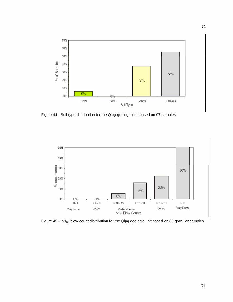
71

71

Figure 44 - Soil-type distribution for the Qlpg geologic unit based on 97 samples

Figure 45 – N160 blow-count distribution for the Qlpg geologic unit based on 89 granular samples

72

72

Figure 46 - Soil-type distribution for the Qlbg geologic unit based on 100 samples

Figure 47 - N160 blow-count distribution for the Qlbg geologic unit based on 78 granular samples

73

73

Figure 48 - Soil-type distribution for the Qlbs geologic unit based on 612 samples

Figure 49 - N160 blow-count distribution for the Qlbs geologic unit based on 301 granular samples

74

74

Figure 50 – Plastic-index distribution in the Qlbs geologic unit based on 29 fine soil samples

Figure 51 - Soil-type distribution for the Qlbm geologic unit based on 176 samples

75

75

Figure 52 - Blow-count distribution for the Qlbm geologic unit based on 10 granular samples

Figure 53 – Plastic-index distribution in the Qlbm geologic unit based on 33 fine soil samples

76

76

Figure 54 - Soil-type distribution for the Qlbpg geologic unit based on 91 samples

Figure 55 - N160 blow-count distribution for the Qlbpg geologic unit based on 79 granular samples

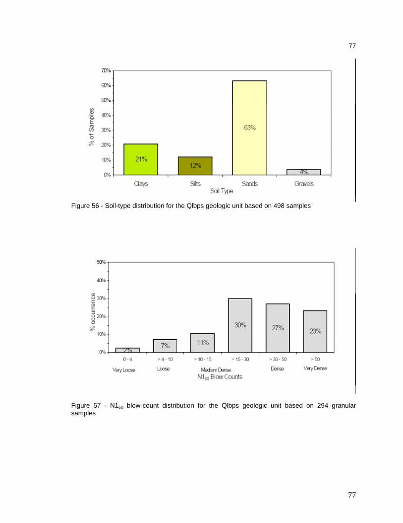
77

77

Figure 56 - Soil-type distribution for the Qlbps geologic unit based on 498 samples

Figure 57 - N160 blow-count distribution for the Qlbps geologic unit based on 294 granular samples

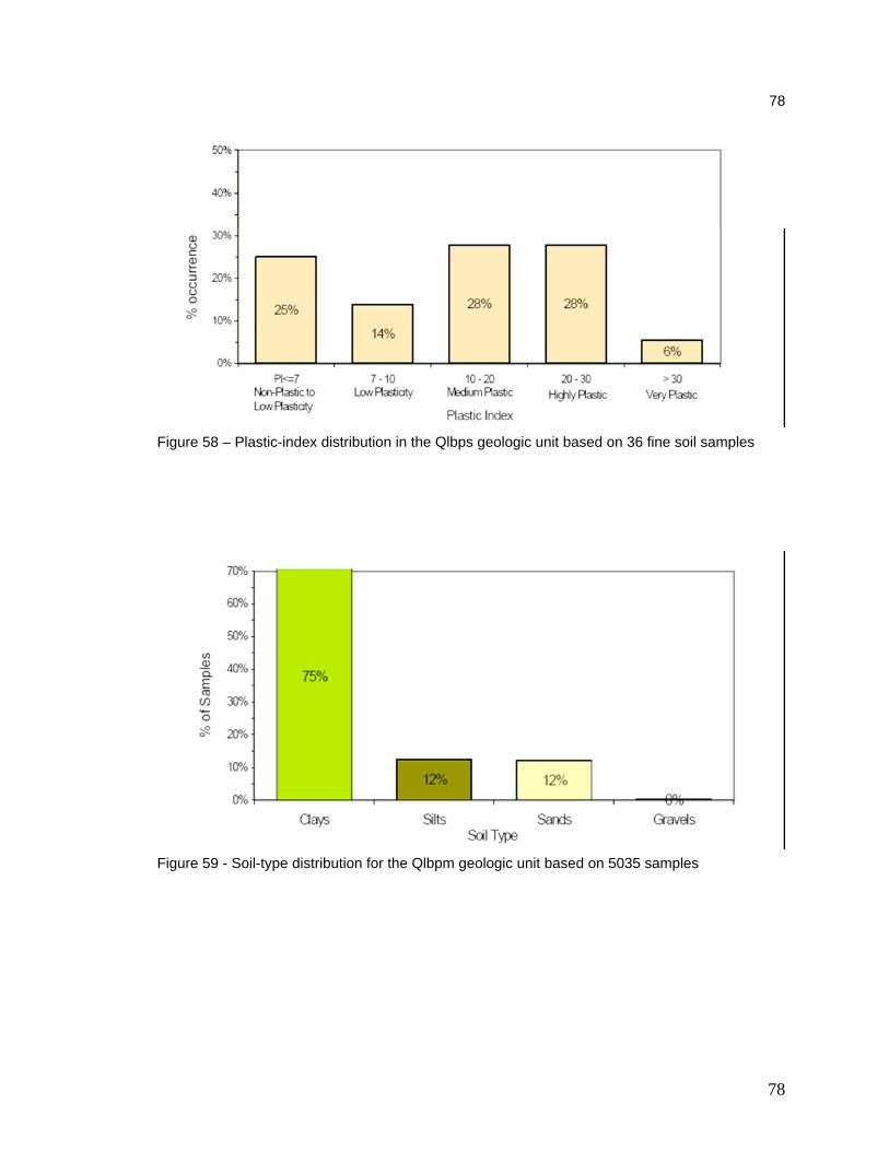
78

78

Figure 58 – Plastic-index distribution in the Qlbps geologic unit based on 36 fine soil samples

Figure 59 - Soil-type distribution for the Qlbpm geologic unit based on 5035 samples

79

79

Figure 60 - N160 blow-count distribution for the Qlbpm geologic unit based on 414 granular samples

Figure 61 – Plastic-index distribution in the Qlbpm geologic unit based on 665 fine soil samples

APPENDIX C

VISUAL BASIC FOR APPLICATIONS CODE

81

This section of the appendix contains the code used for the analysis. All code is run through the Microsoft Visual Basic Editor within ArcGIS. Code following an apostrophe is ignored. The comments are in italics. Table of Contents

A. Average Calculator.......................................................................................................…82

B. Average Filler................................................................................................................…91

C. Groundwater Query……………………………………………….………………………….…98

D. Stress Calculator…………………………………………………....…………………………102

E. N160 Calculator…………………………………………………………………………….….111

F. LiqScreener………………………………………………………………………………........119

G. W Finder………………………………………………………………………………………..121

H. SlopeFinder…………………………………………………………………………………….126

I. R Finder……………………………………………………………………………………..….134

J. Acceleration Reader…………………………………………………………………………..139

K. Atrigger…………………………………………………………………………………………143

L. Layer Merger (15 Calculator)………………………………………………………………...151

M. Lateral Spread Calculator…………………………………………………………………….161

N. Lateral Spread Probability Calculator……………………………………………………….168

O. VS Finder……………………………………………………………………………………….172

P. Generic Table Code…………………………………………………………………………...177

Q. Generic Raster Code………………………………………………………………………….181

R. Generic Feature Class Code…………………………………………………………………184

S. Miscellaneous Code…………………………………………………………………………...185

82

A. Average Calculator 'This program calculates averages of Fines content, mean grain size (D50), Dry Unit Weights, 'and Atterberg Limits, as applicable for soil types from the BLOW Table. 'It creates an average table in the database. First, averages are calculated based on soil 'type and geological unit. Then averages are calculated based on soil tyep regardless of 'geological unit. 'This helps fill in the gaps in the dataset so that other routines can run. ' 'Written By Michael J Olsen 'for MS Thesis 'University of Utah 'January 2005 'Last Modified June 24,2005 'Prepares the user form on initialization Public Sub UserForm_Initialize() 'Set the file name defaults for the combo boxes cboDbFile.AddItem "C:\liq\Liquefaction Database.mdb" cboDbFile.Value = "C:\liq\Liquefaction Database.mdb" End Sub Private Sub Cancel_Click() frmaveragecalc.Hide End Sub Private Sub cmdDbFileSearch_Click() 'This Subroutine changes the location and name of the database to whatever 'the user selects. 'it calls the pLocateData subroutine. Dim DatabaseFilePath As String DatabaseFilePath = pLocateData("Choose the Database", "Database", cboDbFile) 'Adds and Sets the Value of the Combo box to the user's selection. frmaveragecalc.cboDbFile.AddItem DatabaseFilePath frmaveragecalc.cboDbFile.Value = DatabaseFilePath End Sub 'This is the main subroutine of the user form when the user chooses to run the code. Private Sub cmdaveragecalc_Click() 'Open and Set up the Blow Table 'Blow Database File location and Name Dim MDBName As String MDBName = frmaveragecalc.cboDbFile.Value 'Sets up All Values associated with the Blow Table Dim TblBLOWName As String TblBLOWName = "BLOW" 'Opens the table

83

Dim TblBlow As ITable Set TblBlow = OpenTheTable(MDBName, TblBLOWName) 'Gets indexes for the fields necessary for the averaging. Dim TblBlowUSCSFieldNo As Long TblBlowUSCSFieldNo = TblBlow.FindField("USCS") Dim TblBlowgeoFieldNo As Long TblBlowgeoFieldNo = TblBlow.FindField("geolunit") Dim TblBlowDryUnitFieldNo As Long TblBlowDryUnitFieldNo = TblBlow.FindField("DRYUNIT") TblBlowDRYUNITESTFieldNo = TblBlow.FindField("ESTDRY") TblBlowFINESFieldNo = TblBlow.FindField("FINES") TblBlowFINESESTFieldNo = TblBlow.FindField("ESTFINES") TblBlowD50FieldNo = TblBlow.FindField("D50") TblBlowD50ESTFieldNo = TblBlow.FindField("D50EST") TblBlowLiquidLimitFieldNo = TblBlow.FindField("LIQUIDLIMIT") TblBlowPlasticLimitFieldNo = TblBlow.FindField("PLASTICLIMIT") TblBlowPlasticIndexFieldNo = TblBlow.FindField("PLASTICINDEX") TblBlowESTATTFieldNo = TblBlow.FindField("ESTATT") 'Sets up the Cursor to move through the Blow table. Dim TblBlowCursor As ICursor Dim TblBlowFeature As IRowBuffer ' Creates the Average Table and Adds the appropriate fields Dim TblAverage As ITable Set TblAverage = CreateTheTable(MDBName, "AverageTable") 'Use this if the table already exists 'Set TblAverage = OpenTheTable(MDBName, "AverageTable") 'Adds fields to the Average Table, as necessary Call AddField(TblAverage, "geolunit", esriFieldTypeString) Call AddField(TblAverage, "USCS", esriFieldTypeString) Call AddField(TblAverage, "DRYUNIT", esriFieldTypeDouble) Call AddField(TblAverage, "DRYUNITNR", esriFieldTypeInteger) Call AddField(TblAverage, "FINES", esriFieldTypeDouble) Call AddField(TblAverage, "FINESNR", esriFieldTypeInteger) Call AddField(TblAverage, "D50", esriFieldTypeDouble) Call AddField(TblAverage, "D50NR", esriFieldTypeInteger) Call AddField(TblAverage, "LIQUIDLIMIT", esriFieldTypeDouble) Call AddField(TblAverage, "LIQUIDLIMITNR", esriFieldTypeInteger) Call AddField(TblAverage, "PLASTICLIMIT", esriFieldTypeDouble) Call AddField(TblAverage, "PLASTICLIMITNR", esriFieldTypeInteger) Call AddField(TblAverage, "PLASTICINDEX", esriFieldTypeDouble) Call AddField(TblAverage, "PLASTICINDEXNR", esriFieldTypeInteger) 'Sets up indicies for those fields. TblAverageGEOLUNITFieldNo = TblAverage.FindField("GEOLUNIT") TblAverageUSCSFieldNo = TblAverage.FindField("USCS") TblAverageDRYUNITFieldNo = TblAverage.FindField("DRYUNIT") TblAverageDRYUNITNRFieldNo = TblAverage.FindField("DRYUNITNR") TblAverageFINESFieldNo = TblAverage.FindField("FINES") TblAverageFinesNRFieldNo = TblAverage.FindField("FINESNR")

84

TblAverageD50FieldNo = TblAverage.FindField("D50") TblAverageD50NRFieldNo = TblAverage.FindField("D50NR") TblAverageLIQUIDLIMITFieldNo = TblAverage.FindField("LIQUIDLIMIT") TblAverageLiquidLimitNRFieldNo = TblAverage.FindField("LIQUIDLIMITNR") TblAveragePlasticLimitFieldNo = TblAverage.FindField("PLASTICLIMIT") TblAveragePlasticLimitNRFieldNo = TblAverage.FindField("PLASTICLIMITNR") TblAveragePlasticIndexFieldNo = TblAverage.FindField("PLASTICINDEX") TblAveragePlasticIndexNRFieldNo = TblAverage.FindField("PLASTICINDEXNR") 'Sets up a cursor to move through the table. Dim TblAverageUpCursor As ICursor Set TblAverageUpCursor = TblAverage.Update(Nothing, False) 'This is used for creating the rows and updating the values 'once the average is computed. Dim pRow As IRow Set pRow = TblAverage.CreateRow 'creates rows for each new record. 'Various variables used in the loops Dim GeologyUnit As String 'keeps track of the current geological unit Dim SoilType As String 'keeps track of the current Soil Type Dim i As Integer 'loop counter Dim DryUnitWeight As Double 'current Dry Unit Weight Dim fines As Double 'current Fines content Dim D50 As Double 'current D50 value Dim LiquidLimit As Double 'current LL Dim PlasticLimit As Double 'current PL Dim PlasticIndex As Double 'current PI 'This first for loop cycles through the various geological units. For i = 1 To 25 'sets up each round of the loop for different geological units. 'Adjust as necessary. If i = 1 Then GeologyUnit = "ALL" ElseIf i = 2 Then GeologyUnit = "Qaf2" ElseIf i = 3 Then GeologyUnit = "Qafb" ElseIf i = 4 Then GeologyUnit = "Qafo" ElseIf i = 5 Then GeologyUnit = "Qafy" ElseIf i = 6 Then GeologyUnit = "Qal1" ElseIf i = 7 Then GeologyUnit = "Qal2" ElseIf i = 8 Then GeologyUnit = "Qalo" ElseIf i = 9 Then GeologyUnit = "Qalp" ElseIf i = 10 Then GeologyUnit = "Qaly"

85

ElseIf i = 11 Then GeologyUnit = "ca" ElseIf i = 12 Then GeologyUnit = "Qf" ElseIf i = 13 Then GeologyUnit = "Qlaly" ElseIf i = 14 Then GeologyUnit = "Qlbg" ElseIf i = 15 Then GeologyUnit = "Qlbm" ElseIf i = 16 Then GeologyUnit = "Qlbpg" ElseIf i = 17 Then GeologyUnit = "Qlbpm" ElseIf i = 18 Then GeologyUnit = "Qlbps" ElseIf i = 19 Then GeologyUnit = "Qlbs" ElseIf i = 20 Then GeologyUnit = "Qlpg" ElseIf i = 21 Then GeologyUnit = "Qlps" ElseIf i = 22 Then GeologyUnit = "Qly" ElseIf i = 23 Then GeologyUnit = "Qtaf" ElseIf i = 24 Then GeologyUnit = "rock" 'groups several geological units, all nonliquefiable ElseIf i = 25 Then GeologyUnit = "none" 'use in the case geological units haven't been assigned. End If 'The second for loop cycles through all Soil Types in the database. 'Add As necessary. For j = 1 To 60 'change as soil types are added. If j = 1 Then SoilType = "CH" ElseIf j = 2 Then SoilType = "CH-SC" ElseIf j = 3 Then SoilType = "CH-CL" ElseIf j = 4 Then SoilType = "CH-SP" ElseIf j = 5 Then SoilType = "CL" ElseIf j = 6 Then SoilType = "CL-SM" ElseIf j = 7 Then SoilType = "CL-CH" ElseIf j = 8 Then SoilType = "CL-SC" ElseIf j = 9 Then SoilType = "CL-GC"

86

ElseIf j = 10 Then SoilType = "CL-ML" ElseIf j = 11 Then SoilType = "CL-SP" ElseIf j = 12 Then SoilType = "GC" ElseIf j = 13 Then SoilType = "GM" ElseIf j = 14 Then SoilType = "GM-CL" ElseIf j = 15 Then SoilType = "GM-GP" ElseIf j = 16 Then SoilType = "GM-ML" ElseIf j = 17 Then SoilType = "GM-SM" ElseIf j = 18 Then SoilType = "GP-GM" ElseIf j = 19 Then SoilType = "GP-SP" ElseIf j = 20 Then SoilType = "GP-CL" ElseIf j = 21 Then SoilType = "GP-GC" ElseIf j = 22 Then SoilType = "GW" ElseIf j = 23 Then SoilType = "GW-CL" ElseIf j = 24 Then SoilType = "GW-GM" ElseIf j = 25 Then SoilType = "MH" ElseIf j = 26 Then SoilType = "ML" ElseIf j = 27 Then SoilType = "ML-CL" ElseIf j = 28 Then SoilType = "ML-SM" ElseIf j = 29 Then SoilType = "ML-SP" ElseIf j = 30 Then SoilType = "OH" ElseIf j = 31 Then SoilType = "OL" ElseIf j = 32 Then SoilType = "PT" ElseIf j = 33 Then SoilType = "SC" ElseIf j = 34 Then SoilType = "SC-CH" ElseIf j = 35 Then SoilType = "SC-CL" ElseIf j = 36 Then SoilType = "SC-GC"

87

ElseIf j = 37 Then SoilType = "SC-ML" ElseIf j = 38 Then SoilType = "SC-SM" ElseIf j = 39 Then SoilType = "SC-CL" ElseIf j = 40 Then SoilType = "SM" ElseIf j = 41 Then SoilType = "SM-ML" ElseIf j = 42 Then SoilType = "SM-CL" ElseIf j = 43 Then SoilType = "SM-GM" ElseIf j = 44 Then SoilType = "SM-SP" ElseIf j = 45 Then SoilType = "SP" ElseIf j = 46 Then SoilType = "SP-CL" ElseIf j = 47 Then SoilType = "SP-ML" ElseIf j = 48 Then SoilType = "SP-GM" ElseIf j = 49 Then SoilType = "SP-GP" ElseIf j = 50 Then SoilType = "SP-SC" ElseIf j = 51 Then SoilType = "SP-SM" ElseIf j = 52 Then SoilType = "SP-SW" ElseIf j = 53 Then SoilType = "SW" ElseIf j = 54 Then SoilType = "SW-CL" ElseIf j = 55 Then SoilType = "SW-SM" ElseIf j = 56 Then SoilType = "SW-SC" ElseIf j = 57 Then SoilType = "GP" ElseIf j = 58 Then SoilType = "Fill" 'I include concrete and asphalt in this group. ElseIf j = 59 Then SoilType = "GW-ML" ElseIf j = 60 Then SoilType = "ML-CH" End If 'This sets up the Filter used in computing averages. 'It filters the table based on Soil Type and Geological Unit Dim pQueryFilter As IQueryFilter

88

Set pQueryFilter = New QueryFilter 'This defines the filter based on if it is the last run (for all 'geological units) or all other runs (a specific geological unit) If i = 1 Or i = 25 Then 'for i = 1 and 25, the filter is only on soil type. pQueryFilter.WhereClause = "USCS = '" & SoilType & "'" Else 'all other records are filtered by soil type and geology unit pQueryFilter.WhereClause = "GEOLUNIT = '" & GeologyUnit & "'" _ & "And USCS = '" & SoilType & "'" End If 'This resets the cursor for every cycle through the loop Set TblBlowCursor = TblBlow.Search(pQueryFilter, True) 'This finds the number of records in the table once it is filtered. 'It is used to determine how many times the program must loop for each 'soil type in each geological unit. Dim TblBlowFilteredNumRecords As Long TblBlowFilteredNumRecords = RecordCountwFilter(TblBlow, pQueryFilter) 'MsgBox (SoilType & TblBlowFilteredNumRecords) 'Begins the averaging if records are present If Not TblBlowFilteredNumRecords = 0 Then For k = 1 To TblBlowFilteredNumRecords 'advances the cursor Set TblBlowFeature = TblBlowCursor.NextRow 'adds up all dry unit weights in the dataset with a quality of 1 If TblBlowFeature.Value(TblBlowDRYUNITESTFieldNo) = 1 _ And Not IsNull(TblBlowFeature.Value(TblBlowDryUnitFieldNo)) Then DryUnitWeight=DryUnitWeight+TblBlowFeature.Value(TblBlowDryUnitFieldNo) nDU = nDU + 1 'keeps track of the # of DUW End If 'adds up all fines in the dataset with a quality of 1 If Not IsNull(TblBlowFeature.Value(TblBlowFINESFieldNo)) _ And TblBlowFeature.Value(TblBlowFINESESTFieldNo) = 1 Then fines = fines + TblBlowFeature.Value(TblBlowFINESFieldNo) nFines = nFines + 1 'keeps track of the # of fines. End If 'adds up all D50's with a quality of 1 If Not IsNull(TblBlowFeature.Value(TblBlowD50FieldNo)) _ And TblBlowFeature.Value(TblBlowD50ESTFieldNo) = 1 Then D50 = D50 + TblBlowFeature.Value(TblBlowD50FieldNo) nD50 = nD50 + 1 End If

89

'adds up all LL w/ a quality of 1 If Not IsNull(TblBlowFeature.Value(TblBlowLiquidLimitFieldNo)) _ And TblBlowFeature.Value(TblBlowESTATTFieldNo) = 1 Then LiquidLimit = LiquidLimit + TblBlowFeature.Value(TblBlowLiquidLimitFieldNo) nLiquidLimit = nLiquidLimit + 1 End If 'adds up all PL with a quality of 1 If Not IsNull(TblBlowFeature.Value(TblBlowPlasticLimitFieldNo)) _ And TblBlowFeature.Value(TblBlowESTATTFieldNo) = 1 Then PlasticLimit = PlasticLimit + TblBlowFeature.Value(TblBlowPlasticLimitFieldNo) nPlasticLimit = nPlasticLimit + 1 End If 'adds up all PI with a quality of 1 If Not IsNull(TblBlowFeature.Value(TblBlowPlasticIndexFieldNo)) _ And TblBlowFeature.Value(TblBlowESTATTFieldNo) = 1 Then PlasticIndex = PlasticIndex+TblBlowFeature.Value(TblBlowPlasticIndexFieldNo) nPlasticIndex = nPlasticIndex + 1 End If Next 'for k loop k = 0 'reset k to zero End If 'If Statements to compute the averages and store them in the Average Table If nDU > 0 Then pRow.Value(TblAverageDRYUNITFieldNo) = DryUnitWeight / nDU pRow.Value(TblAverageDRYUNITNRFieldNo) = nDU pRow.Store End If If nFines > 0 Then pRow.Value(TblAverageFINESFieldNo) = fines / nFines pRow.Value(TblAverageFinesNRFieldNo) = nFines pRow.Store End If If nD50 > 0 Then pRow.Value(TblAverageD50FieldNo) = D50 / nD50 pRow.Value(TblAverageD50NRFieldNo) = nD50 pRow.Store End If If nLiquidLimit > 0 Then pRow.Value(TblAverageLIQUIDLIMITFieldNo) = LiquidLimit / nLiquidLimit pRow.Value(TblAverageLiquidLimitNRFieldNo) = nLiquidLimit pRow.Store End If If nPlasticLimit > 0 Then

90

pRow.Value(TblAveragePlasticLimitFieldNo) = PlasticLimit / nPlasticLimit pRow.Value(TblAveragePlasticLimitNRFieldNo) = nPlasticLimit pRow.Store End If If nPlasticIndex > 0 Then pRow.Value(TblAveragePlasticIndexFieldNo) = PlasticIndex / nPlasticIndex pRow.Value(TblAveragePlasticIndexNRFieldNo) = nPlasticIndex pRow.Store End If 'Reset all values to zero for the next round DryUnitWeight = 0 nDU = 0 fines = 0 nFines = 0 D50 = 0 nD50 = 0 LiquidLimit = 0 nLiquidLimit = 0 PlasticLimit = 0 nPlasticLimit = 0 PlasticIndex = 0 nPlasticIndex = 0 'Reset the cursor for the next loop Set TblBlowCursor = Nothing Set TblBlowFeature = Nothing 'Stores the information of the geolocial units and soil type and 'creates a new row for the next loop through. pRow.Value(TblAverageGEOLUNITFieldNo) = GeologyUnit pRow.Store pRow.Value(TblAverageUSCSFieldNo) = SoilType pRow.Store Set pRow = TblAverage.CreateRow Next 'next for j loop Next 'next for i loop MsgBox ("Average Value Table Created and Populated.") 'closes the program frmaveragecalc.Hide End Sub

91

B. Average Filler 'This program fills in the BLOWFILL table with averages of Fines content, 'mean grain size (D50), Dry Unit Weights, and Atterberg Limits, as applicable 'for soil types in the BLOWFILL Table. 'It first will search for an average from the same soil type and geological unit. 'If this is not available, then it will get the average based on soil type only. 'This helps fill in the gaps in the dataset so that other routines can run. ' 'Before running this routine, the usere should create the table BLOWFILL by copying the BLOW 'Table and naming it BLOWFILL. ' 'Written By Michael J Olsen 'for MS Thesis 'University of Utah 'January 2005 'Last Modified June 24,2005 Public Sub UserForm_Initialize() 'Set the file name defaults for the combo boxes cboDbFile.AddItem "C:\liq\Liquefaction Database.mdb" cboDbFile.Value = "C:\liq\Liquefaction Database.mdb" End Sub Private Sub Cancel_Click() frmAverageFill.Hide End Sub Private Sub cmdDbFileSearch_Click() 'This Subroutine changes the location and name of the database to whatever the user selects. Dim DatabaseFilePath As String DatabaseFilePath = pLocateData("Choose the Database", "Database", cboDbFile) 'Adds and Sets the Value of the Combo box to the user's selection. frmAverageFill.cboDbFile.AddItem DatabaseFilePath frmAverageFill.cboDbFile.Value = DatabaseFilePath End Sub 'This is the main subroutine of the function. Private Sub cmdaveragefill_Click() 'Open and Set up the BlowFill Table 'BlowFill Database File location and Name Dim MDBName As String MDBName = frmAverageFill.cboDbFile.Value 'Sets up All Values associated with the BlowFill Table

92

Dim TblBlowFillName As String TblBlowFillName = "BlowFill" 'This is old code which copies the table. It can be used, but is not recommended, 'as it is very slow and is easily disrupted by errors if the data has issues. 'its best just to use ArcCatalog or Microsoft Access to copy the table first. 'Call CopyTheTable(MDBName, "BLOW", "BLOWFILL") 'MsgBox ("Blowfill Table Created.") 'Opens the table BLOWFILL Dim TblBlowFill As ITable Set TblBlowFill = OpenTheTable(MDBName, TblBlowFillName) 'Sets up indicies for fields Dim TblBlowFillUSCSFieldNo As Long TblBlowFillUSCSFieldNo = TblBlowFill.FindField("USCS") Dim TblBlowFillGeolUnitFieldNo As Long TblBlowFillGeolUnitFieldNo = TblBlowFill.FindField("geolunit") Dim TblBlowFillDRYUNITFieldNo As Long Dim TblBlowFillDRYUNITESTFieldNo As Long Dim TblBlowFillWETUNITFieldNo As Long Dim TblBlowFillWETUNITESTFieldNo As Long Dim TblBlowFillWATERCONTENTFieldNo As Long Dim TblBlowFillFinesFieldNo As Long Dim TblBlowFillFINESESTFieldNo As Long Dim TblBlowFillD50FieldNo As Long Dim TblBlowFillD50ESTFieldNo As Long Dim TblBlowFillLIQUIDLIMITFieldNo As Long Dim TblBlowFillPlasticLimitFieldNo As Long Dim TblBlowFillPlasticIndexFieldNo As Long Dim TblBlowFillESTATTFieldNo As Long Dim TblBlowFillSPGRAVITYFieldNo As Long Dim TblBlowFillESTSPGRFieldNo As Long TblBlowFillDRYUNITFieldNo = TblBlowFill.FindField("DRYUNIT") TblBlowFillDRYUNITESTFieldNo = TblBlowFill.FindField("ESTDRY") TblBlowFillWETUNITFieldNo = TblBlowFill.FindField("WETUNIT") TblBlowFillWETUNITESTFieldNo = TblBlowFill.FindField("ESTWET") TblBlowFillWATERCONTENTFieldNo = TblBlowFill.FindField("MOISTURE_CONTENT") TblBlowFillFinesFieldNo = TblBlowFill.FindField("FINES") TblBlowFillFINESESTFieldNo = TblBlowFill.FindField("ESTFINES") TblBlowFillD50FieldNo = TblBlowFill.FindField("D50") TblBlowFillD50ESTFieldNo = TblBlowFill.FindField("D50EST") TblBlowFillLIQUIDLIMITFieldNo = TblBlowFill.FindField("LIQUIDLIMIT") TblBlowFillPlasticLimitFieldNo = TblBlowFill.FindField("PLASTICLIMIT") TblBlowFillPlasticIndexFieldNo = TblBlowFill.FindField("PLASTICINDEX") TblBlowFillESTATTFieldNo = TblBlowFill.FindField("ESTATT") TblBlowFillSPGRAVITYFieldNo = TblBlowFill.FindField("SPGRAVITY") TblBlowFillESTSPGRFieldNo = TblBlowFill.FindField("ESTSPGR") TblBlowFillESTNMFieldNo = TblBlowFill.FindField("ESTNM")

93

'Sets up the Cursor to move through the BlowFill table. Dim TblBlowFillCursor As ICursor Dim TblBlowFillFeature As IRowBuffer Set TblBlowFillCursor = TblBlowFill.Update(Nothing, False) 'Determines the number of records in the BlowFill table Dim TblBlowFillNumRecords As Long TblBlowFillNumRecords = RecordCountwFilter(TblBlowFill, Nothing) 'Opens up and sets up the Average Table Dim TblAverage As ITable Set TblAverage = OpenTheTable(MDBName, "AverageTable") TblAverageGEOLUNITFieldNo = TblAverage.FindField("GEOLUNIT") TblAverageUSCSFieldNo = TblAverage.FindField("USCS") TblAverageDRYUNITFieldNo = TblAverage.FindField("DRYUNIT") 'TblAverageDRYUNITNRFieldNo = TblAverage.FindField("DRYUNITNR") TblAverageFINESFieldNo = TblAverage.FindField("FINES") 'TblAverageFinesNRFieldNo = TblAverage.FindField("FINESNR") TblAverageD50FieldNo = TblAverage.FindField("D50") 'TblAverageD50NRFieldNo = TblAverage.FindField("D50NR") TblAverageLIQUIDLIMITFieldNo = TblAverage.FindField("LIQUIDLIMIT") 'TblAverageLiquidLimitNRFieldNo = TblAverage.FindField("LIQUIDLIMITNR") TblAveragePlasticLimitFieldNo = TblAverage.FindField("PLASTICLIMIT") 'TblAveragePlasticLimitNRFieldNo = TblAverage.FindField("PLASTICLIMITNR") TblAveragePlasticIndexFieldNo = TblAverage.FindField("PLASTICINDEX") 'TblAveragePlasticIndexNRFieldNo = TblAverage.FindField("PLASTICINDEXNR") 'Sets up a cursor to move through the table. Dim TblAverageCursor As ICursor Dim TblAverageRowBuffer As IRowBuffer Set TblAverageCursor = TblAverage.Search(Nothing, True) Set TblAverageRowBuffer = TblAverageCursor.NextRow 'Various variables used in the loops Dim GeologyUnit As String 'Geological Unit Dim SoilType As String 'Soil Type Dim gammadry As Double 'Dry Unit Weight Dim Watercontent As Double 'water content of the soil Dim i As Integer 'Loop variable 'The Loop that goes through the blowfill table and fills in missing values For i = 1 To TblBlowFillNumRecords 'advances the cursor Set TblBlowFillFeature = TblBlowFillCursor.NextRow 'If statement to see if it is a record that would need averages or not. If IsNull(TblBlowFillFeature.Value(TblBlowFillGeolUnitFieldNo)) _ Or IsNull(TblBlowFillFeature.Value(TblBlowFillUSCSFieldNo)) Then

94

Else GeologyUnit = TblBlowFillFeature.Value(TblBlowFillGeolUnitFieldNo) SoilType = TblBlowFillFeature.Value(TblBlowFillUSCSFieldNo) 'This sets up the Filter used in computing averages. 'It filters the table based on Soil Type and Geological Unit Dim pQueryFilter As IQueryFilter Set pQueryFilter = New QueryFilter 'The second filter is used for where data is from all geological units Dim pQueryFilter2 As IQueryFilter Set pQueryFilter2 = New QueryFilter pQueryFilter.WhereClause = "GEOLUNIT = '" & GeologyUnit & "'" _ & "And USCS = '" & SoilType & "'" pQueryFilter2.WhereClause = "GEOLUNIT = 'ALL'" _ & "And USCS = '" & SoilType & "'" 'counts the records in the average table with the filter based on 'soil type and geological unit TblAverageNumRecords = RecordCountwFilter(TblAverage, pQueryFilter) 'counts the records in the average table with the filter based on 'soil type only TblAverageNumRecords2 = RecordCountwFilter(TblAverage, pQueryFilter2) 'Sets the Cursor to the appropriate location Set TblAverageCursor = TblAverage.Search(pQueryFilter, True) Set TblAverageRowBuffer = TblAverageCursor.NextRow 'Used for samples not assigned a geological unit to ensure that the 'estimate quality is 5 not 4. If TblBlowFillFeature.Value(TblBlowFillGeolUnitFieldNo) = "none" Then DQ = 5 Else DQ = 4 End If 'Begins the analysis if there is only 1 record for that soil type, ensures 'there are no duplicates. If TblAverageNumRecords = 1 Then 'Fills in the Dry Unit Weight Field with an average if the record does 'not have one. If IsNull(TblBlowFillFeature.Value(TblBlowFillDRYUNITFieldNo)) Then If Not IsNull(TblAverageRowBuffer.Value(TblAverageDRYUNITFieldNo)) Then TblBlowFillFeature.Value(TblBlowFillDRYUNITFieldNo) = _ TblAverageRowBuffer.Value(TblAverageDRYUNITFieldNo) TblBlowFillFeature.Value(TblBlowFillDRYUNITESTFieldNo) = DQ Else

95

Set TblAverageCursor = TblAverage.Search(pQueryFilter2, True) Set TblAverageRowBuffer = TblAverageCursor.NextRow TblBlowFillFeature.Value(TblBlowFillDRYUNITFieldNo) = _ TblAverageRowBuffer.Value(TblAverageDRYUNITFieldNo) TblBlowFillFeature.Value(TblBlowFillDRYUNITESTFieldNo) = 5 End If End If 'Calculates WetUnitWeight where null in database and where moisture content 'information is available. If IsNull(TblBlowFillFeature.Value(TblBlowFillWETUNITFieldNo)) Then If Not IsNull(TblBlowFillFeature.Value(TblBlowFillWATERCONTENTFieldNo)) _ And Not IsNull(TblBlowFillFeature.Value(TblBlowFillDRYUNITFieldNo)) Then gammadry = TblBlowFillFeature.Value(TblBlowFillDRYUNITFieldNo) Watercontent =TblBlowFillFeature.Value(TblBlowFillWATERCONTENTFieldNo) / 100 TblBlowFillFeature.Value(TblBlowFillWETUNITFieldNo) = _ gammadry * (1 + Watercontent) TblBlowFillFeature.Value(TblBlowFillWETUNITESTFieldNo) = _ TblBlowFillFeature.Value(TblBlowFillDRYUNITESTFieldNo) End If End If 'Fills in the Fines Field with an average if the record does not have a value If IsNull(TblBlowFillFeature.Value(TblBlowFillFinesFieldNo)) Then If Not IsNull(TblAverageRowBuffer.Value(TblAverageFINESFieldNo)) Then TblBlowFillFeature.Value(TblBlowFillFinesFieldNo) = _ TblAverageRowBuffer.Value(TblAverageFINESFieldNo) TblBlowFillFeature.Value(TblBlowFillFINESESTFieldNo) = DQ Else Set TblAverageCursor = TblAverage.Search(pQueryFilter2, True) Set TblAverageRowBuffer = TblAverageCursor.NextRow TblBlowFillFeature.Value(TblBlowFillFinesFieldNo) = _ TblAverageRowBuffer.Value(TblAverageFINESFieldNo) TblBlowFillFeature.Value(TblBlowFillFINESESTFieldNo) = 5 End If End If 'Fills in the D50 Field with an average if the record does not have a value If IsNull(TblBlowFillFeature.Value(TblBlowFillD50FieldNo)) Then If Not IsNull(TblAverageRowBuffer.Value(TblAverageD50FieldNo)) Then TblBlowFillFeature.Value(TblBlowFillD50FieldNo) = _ TblAverageRowBuffer.Value(TblAverageD50FieldNo) TblBlowFillFeature.Value(TblBlowFillD50ESTFieldNo) = DQ Else Set TblAverageCursor = TblAverage.Search(pQueryFilter2, True) Set TblAverageRowBuffer = TblAverageCursor.NextRow TblBlowFillFeature.Value(TblBlowFillD50FieldNo) = _ TblAverageRowBuffer.Value(TblAverageD50FieldNo) TblBlowFillFeature.Value(TblBlowFillD50ESTFieldNo) = 5

96

End If End If 'If the soil could be plastic, then averages are computed.

If SoilType = "CL" Or SoilType = "CH" Or SoilType = "CL-CH" Or SoilType = "CH-CL" _ Or SoilType = "OH" Or SoilType = "CH" Or SoilType = "Pt" Or SoilType = "OL-CL" _

Or SoilType = "CL-OL" Then If IsNull(TblBlowFillFeature.Value(TblBlowFillLIQUIDLIMITFieldNo)) Then If Not IsNull(TblAverageRowBuffer.Value(TblAverageLIQUIDLIMITFieldNo)) Then TblBlowFillFeature.Value(TblBlowFillLIQUIDLIMITFieldNo) = _ TblAverageRowBuffer.Value(TblAverageLIQUIDLIMITFieldNo) TblBlowFillFeature.Value(TblBlowFillESTATTFieldNo) = DQ Else Set TblAverageCursor = TblAverage.Search(pQueryFilter2, True) Set TblAverageRowBuffer = TblAverageCursor.NextRow TblBlowFillFeature.Value(TblBlowFillLIQUIDLIMITFieldNo) = _ TblAverageRowBuffer.Value(TblAverageLIQUIDLIMITFieldNo) TblBlowFillFeature.Value(TblBlowFillESTATTFieldNo) = 5 End If End If If IsNull(TblBlowFillFeature.Value(TblBlowFillPlasticLimitFieldNo)) Then If Not IsNull(TblAverageRowBuffer.Value(TblAveragePlasticLimitFieldNo)) Then TblBlowFillFeature.Value(TblBlowFillPlasticLimitFieldNo) = _ TblAverageRowBuffer.Value(TblAveragePlasticLimitFieldNo) TblBlowFillFeature.Value(TblBlowFillESTATTFieldNo) = DQ Else Set TblAverageCursor = TblAverage.Search(pQueryFilter2, True) Set TblAverageRowBuffer = TblAverageCursor.NextRow TblBlowFillFeature.Value(TblBlowFillPlasticLimitFieldNo) = _ TblAverageRowBuffer.Value(TblAveragePlasticLimitFieldNo) TblBlowFillFeature.Value(TblBlowFillESTATTFieldNo) = 5 End If End If If IsNull(TblBlowFillFeature.Value(TblBlowFillPlasticIndexFieldNo)) Then If Not IsNull(TblAverageRowBuffer.Value(TblAveragePlasticIndexFieldNo)) Then TblBlowFillFeature.Value(TblBlowFillPlasticIndexFieldNo) = _ TblAverageRowBuffer.Value(TblAveragePlasticIndexFieldNo) TblBlowFillFeature.Value(TblBlowFillESTATTFieldNo) = DQ Else Set TblAverageCursor = TblAverage.Search(pQueryFilter2, True) Set TblAverageRowBuffer = TblAverageCursor.NextRow TblBlowFillFeature.Value(TblBlowFillPlasticIndexFieldNo) = _ TblAverageRowBuffer.Value(TblAveragePlasticIndexFieldNo) TblBlowFillFeature.Value(TblBlowFillESTATTFieldNo) = 5 End If End If End If 'Plastic Soil Types End of If Statement

97

'This puts in default values of the specific gravity for records that do not have 'Specific Gravities. If the soil type is not listed, then a typical value of 2.7 is used. If IsNull(TblBlowFillFeature.Value(TblBlowFillSPGRAVITYFieldNo)) Then If SoilType = "CL" Or SoilType = "CH" Then SpecGrav = 2.75 ElseIf SoilType = "SM" Or SoilType = "SP" Or SoilType = "SW" _ Or SoilType = "SC" Or SoilType = "GC" Or SoilType = "GM" _ Or SoilType = "GM-GP" Or SoilType = "GM-SM" Or SoilType = "GP" _ Or SoilType = "SM-GM" Or SoilType = "SM-SP" Or SoilType = "SP-GM" _ Or SoilType = "SP-GP" Or SoilType = "SP-SC" Or SoilType = "SP-SM" _ Or SoilType = "SP-SW" Or SoilType = "SW" Or SoilType = "SW-SM" _ Or SoilType = "SW-SC" Then SpecGrav = 2.65 Else SpecGrav = 2.7 End If 'End if to Specific Gravity Assignment if Statement. TblBlowFillFeature.Value(TblBlowFillSPGRAVITYFieldNo) = SpecGrav TblBlowFillFeature.Value(TblBlowFillESTSPGRFieldNo) = 3 End If 'End if to Specific Gravity If Statement End If 'End of If for 1 record in average table End If 'End if to each record with USCS or GeolUnit

'Eliminates zero length strings in the ESTNM Field. It was causing an error. They are ‘flagged with a 9.

If TblBlowFillFeature.Value(TblBlowFillESTNMFieldNo) = "" Then TblBlowFillFeature.Value(TblBlowFillESTNMFieldNo) = "9" End If 'Updates the database TblBlowFillCursor.UpdateRow TblBlowFillFeature 'Resets the average cursor Set TblAverageCursor = Nothing Set TblAverageRowBuffer = Nothing DQ = 4 Next i 'next for i loop 'closes the program MsgBox ("Average Values Added Successfully to Database.") frmAverageFill.Hide End Sub

98

C. GROUNDWATER QUERY 'This program inputs a groundwater grid which can be created using 'ArcGIS Spatial Analyst or 3D analyst by interpolation with the Sites that 'have recorded groundwater depths. 'The program uses that grid for estimates of groundwater depth at sites which 'do not have recorded ground water depths. ' 'NOTE: The groundwater grid and Site Feature Class must use the same coordinate system. 'For this project, UTM NAD 83 Zone 12 North was used ' 'If the user wants to run the groundwater query for just select points, then they 'must select the points first using the ArcGIS Select Tool (for the Site layer only) 'Make sure that the points are only selected from the SITE layer and no other layers. ' 'Written by Michael J. Olsen 'MS Thesis 'University of Utah 'September, 2004 ' 'Last Modified: June 24, 2005 'Option Explicit Private Sub UserForm_Initialize() 'Set the file name defaults for the combo boxes cboLiqDbFile.AddItem "C:\liq\Liquefaction Database.mdb" cboLiqDbFile.Value = "C:\liq\Liquefaction Database.mdb" cboGWGridFile.AddItem "C:\liq\GWGrid" cboGWGridFile.Value = "C:\liq\GWGrid" 'Sets up the program for all records or selected records. cboGWSelect.AddItem "<ALL RECORDS>" cboGWSelect.AddItem "Selected" cboGWSelect.Value = "<ALL RECORDS>" End Sub Private Sub Cancel_Click() frmGroundwaterQuery.Hide End Sub Private Sub cmdLiqDbFileSearch_Click() 'This Subroutine changes the location and name of the database to whatever the user selects. Dim DatabaseFilePath As String DatabaseFilePath = pLocateData("Choose the Database", "Database", cboLiqDbFile) 'Adds the values to the combobox frmGroundwaterQuery.cboLiqDbFile.AddItem DatabaseFilePath frmGroundwaterQuery.cboLiqDbFile.Value = DatabaseFilePath End Sub Private Sub cmdGWGridFileSearch_Click() 'This Subroutine changes the location and name of the 'Groundwater database to whatever the user selects.

99

Dim GWGridFilePath As String GWGridFilePath = pLocateData("Choose the Ground water Grid Map", "Raster", cboGWGridFile) 'Adds the values to the combobox. frmGroundwaterQuery.cboGWGridFile.AddItem GWGridFilePath frmGroundwaterQuery.cboGWGridFile.Value = GWGridFilePath End Sub Private Sub cmdGWFinder_Click() 'This is the main routine which finds a value for the Groundwater 'Depth based on a previously created interpolated grid (gwgrid) 'Opens up the Site Table. 'Site Database File location and Name Dim MDBName As String MDBName = frmGroundwaterQuery.cboLiqDbFile.Value 'Sets up All Values associated with the Site Table Dim TblSITENAME As String TblSITENAME = "SITE" 'Dim TblSiteFeatureClass As ITable 'Set TblSiteFeatureClass = OpenTheTable(MDBName, TblSiteFeatureClassName) 'Set up the Cursor to move through the Site Table 'Opens the Access File and Table Dim pDBWorkspaceFactory As IWorkspaceFactory Dim pDBWS As IFeatureWorkspace Set pDBWorkspaceFactory = New AccessWorkspaceFactory Set pDBWS = pDBWorkspaceFactory.OpenFromFile(MDBName, 0) Dim TblSiteFeatureClass As IFeatureClass Set TblSiteFeatureClass = pDBWS.OpenFeatureClass("SITE") 'Sets up variables to find the necessary fields of the database table. Dim TblSiteFeatureClassSITEIDNo As Long TblSiteFeatureClassSITEIDNo = TblSiteFeatureClass.FindField("SITEIDNO") Dim TblSiteFeatureClassxFieldNo As Long TblSiteFeatureClassxFieldNo = TblSiteFeatureClass.FindField("Easting") Dim TblSiteFeatureClassyFieldNo As Long TblSiteFeatureClassyFieldNo = TblSiteFeatureClass.FindField("Northing") Call AddField(TblSiteFeatureClass, "DepthGW", esriFieldTypeDouble) Dim TblSiteFeatureClassGWFieldNo As Long TblSiteFeatureClassGWFieldNo = TblSiteFeatureClass.FindField("DepthGW") Call AddField(TblSiteFeatureClass, "GWEST", esriFieldTypeSmallInteger) Dim TblSiteFeatureClassGWEstFieldNo As Long TblSiteFeatureClassGWEstFieldNo = TblSiteFeatureClass.FindField("GWEST") Dim TblSiteFeatureClassNumRecords As Integer TblSiteFeatureClassNumRecords = RecordCount(TblSiteFeatureClass) 'Sets up the filter for querying the database Dim pFilter As IQueryFilter

100

Set pFilter = New QueryFilter 'Sets up A Cursor to go through the desired records. Dim pFCursor As IFeatureCursor Dim TblSiteSelectionSet As ISelectionSet2 Dim NumRecords As Integer 'Sets up the routine based on if it is for a selection or for the entier dataset. If cboGWSelect = "Selected" Then Set TblSiteSelectionSet = selectfeaturesfrommap(TblSITENAME) If TblSiteSelectionSet Is Nothing Then GoTo ExitRoutine End If TblSiteSelectionSet.Update Nothing, True, pFCursor 'Counts the number of records based on the selection NumRecords = TblSiteSelectionSet.Count Else Set pFCursor = TblSiteFeatureClass.Search(Nothing, True) NumRecords = TblSiteFeatureClass.FeatureCount(Nothing) End If 'If the User hasn't selected anything but chose selected, then the routine 'must be exited so that the User can select the records. If NumRecords = 0 Then MsgBox ("Select Features from Map and Re-run Groundwater Query") GoTo ExitRoutine End If 'Sets up the cursors Dim TblSiteSelectedSearchFeature As IFeature Dim TblSiteUpCursor As IFeatureCursor Dim TblSiteUpFeature As IFeature Set TblSiteUpCursor = TblSiteFeatureClass.Update(Nothing, True) 'Opens the GWGrid 'Name and Path Of GWGrid Dim pGWFilePath As String pGWFilePath = FilePathFinder(frmGroundwaterQuery.cboGWGridFile.Value) Dim pGWFileName As String pGWFileName = FileNameFinder(frmGroundwaterQuery.cboGWGridFile.Value) 'Opens the GWGrid Rasterlayer Dim pGWGridLayer As IRasterLayer Set pGWGridLayer = OpenRasterLayer(pGWFilePath, pGWFileName) 'Sets up the variables used in the loop 'These are the x and y coordinates of the site Dim xSite As Double Dim ySite As Double Dim gw As Double 'gw is the depth read off of the groundwater grid 'This is the counter for the for loop

101

Dim i As Integer 'This is the query filter used when the user has made a selection rather 'than finding groundwater values for every record in the database Dim pIDfilter As IQueryFilter Set pIDfilter = New QueryFilter 'The main loop of the function to cycle through the Site Records For i = 1 To NumRecords If cboGWSelect = "Selected" Then Set TblSiteSelectedSearchFeature = pFCursor.NextFeature pOid = TblSiteSelectedSearchFeature.Value(TblSiteFeatureClassSITEIDNo) pIDfilter.WhereClause = "SITEIDNO = " & pOid Set TblSiteUpCursor = Nothing Set TblSiteUpCursor = TblSiteFeatureClass.Update(pIDfilter, True) End If 'advances 1 record. Set TblSiteUpFeature = TblSiteUpCursor.NextFeature 'Gets the coordinates of the site from the site table. xSite = TblSiteUpFeature.Value(TblSiteFeatureClassxFieldNo) ySite = TblSiteUpFeature.Value(TblSiteFeatureClassyFieldNo) 'Ensures that no GW values are overwritten If IsNull(TblSiteUpFeature.Value(TblSiteFeatureClassGWFieldNo)) Then 'Reads Values from Groundwater Grid using the subroutine GRIDREADER gw = GridReader(xSite, ySite, pGWGridLayer) 'Writes the values to the database. Also returns the 'dataqualifier of 3 TblSiteUpFeature.Value(TblSiteFeatureClassGWEstFieldNo) = 3 'Updates the Groundwater Field TblSiteUpFeature.Value(TblSiteFeatureClassGWFieldNo) = gw TblSiteUpCursor.UpdateFeature TblSiteUpFeature End If 'Moves on to the next record to find the groundwater depth. Next 'Informs the User that the program has executed successfully MsgBox ("Groundwater Depth Values Added Successfully to Database.") ExitRoutine: 'closes the UserForm frmGroundwaterQuery.Hide End Sub

102

D. STRESS CALCULATOR 'This program will calculate the effective and total stresses for a soil profile. 'It requires a database with a table SITE with Site information (GWDepth) and 'a table BLOWfill which has the soil profile information, unit weights, & Specific Gravity. 'This is the table created in the AverageFill Routine from the BLOW table. 'As a bare minimum, each entry must have a depth value recorded. Then if the layer is not 'designated by a Boolean True for the Boundary Field, then it must have a DryUnit Weight and 'a Specific Gravity in order for the program to function. 'This program assumes that the DRYUnit weight is in kn/m^3 and the depth is in ft. 'If the DRYUnit weight is in pcf, then change Conv to 1... ' 'Written By Michael J Olsen 'University of Utah 'January 17, 2005 ' 'Last Modified: June 24, 2005 Option Explicit Public Sub UserForm_Initialize() 'Set the file name defaults for the combo boxes cboDbFile.AddItem "C:\liq\Liquefaction Database.mdb" cboDbFile.Value = "C:\liq\Liquefaction Database.mdb" End Sub Private Sub Cancel_Click() frmeffstresscalc.Hide End Sub Private Sub cmdDbFileSearch_Click() 'This Subroutine changes the location and name of the database to whatever the user selects. Dim DatabaseFilePath As String DatabaseFilePath = pLocateData("Choose the Database", "Database", cboDbFile) 'Adds and Sets the Value of the Combo box to the user's selection. frmeffstresscalc.cboDbFile.AddItem DatabaseFilePath frmeffstresscalc.cboDbFile.Value = DatabaseFilePath End Sub Private Sub cmdeffstresscalc_Click() 'The main subroutine of the user form when the user clicks run. 'Database which contains the tables. Taken from the ComboBox on the UserForm Dim MDBName As String MDBName = frmeffstresscalc.cboDbFile.Value 'SETUP for the Blow Table

103

'Blow Database File location and Name Dim TblBlowFillName As String TblBlowFillName = "BLOWFill" 'Opens the table Dim TblBlowFill As ITable Set TblBlowFill = OpenTheTable(MDBName, TblBlowFillName) 'Adds the fields to store the Total and Effective Stress Values Call AddField(TblBlowFill, "TotalStress", esriFieldTypeDouble) Call AddField(TblBlowFill, "EffectiveStress", esriFieldTypeDouble) Call AddField(TblBlowFill, "MoistUnitWeight", esriFieldTypeDouble) Call AddField(TblBlowFill, "SatUnitWeight", esriFieldTypeDouble) Call AddField(TblBlowFill, "ObjectID", esriFieldTypeOID) Call AddField(TblBlowFill, "ErrorDUWorGS", esriFieldTypeSingle) 'Gets Field Location Values for fields it needs to read from and update. Dim TblBlowFillTotalStressFieldNo As Long TblBlowFillTotalStressFieldNo = TblBlowFill.FindField("TotalStress") Dim TblBlowFillEffectiveStressFieldNo As Long TblBlowFillEffectiveStressFieldNo = TblBlowFill.FindField("EffectiveStress") Dim TblBlowFillMoistUnitWeightFieldNo As Long TblBlowFillMoistUnitWeightFieldNo = TblBlowFill.FindField("MoistUnitWeight") Dim TblBlowFillSatUnitWeightFieldNo As Long TblBlowFillSatUnitWeightFieldNo = TblBlowFill.FindField("SatUnitWeight") Dim TblBlowFillErrorFieldNo As Long TblBlowFillErrorFieldNo = TblBlowFill.FindField("ErrorDUWorGS") Dim TblBlowFillDRYUNITFieldNo As Long TblBlowFillDRYUNITFieldNo = TblBlowFill.FindField("DryUnit") Dim TblBlowFillWETUNITFieldNo As Long TblBlowFillWETUNITFieldNo = TblBlowFill.FindField("WetUnit") Dim TblBlowFillDepthFieldNo As Long TblBlowFillDepthFieldNo = TblBlowFill.FindField("Depth") Dim TblBlowFillGSFieldNo As Long TblBlowFillGSFieldNo = TblBlowFill.FindField("SPGRAVITY") Dim TblBlowFillBoundaryFieldNo As Long TblBlowFillBoundaryFieldNo = TblBlowFill.FindField("Boundary") Dim TblBlowFillSITEIDNoFieldNo As Long TblBlowFillSITEIDNoFieldNo = TblBlowFill.FindField("SITEIDNO") 'SETUP for the SiteTable Dim TblSITENAME As String TblSITENAME = "SITE"

104

'Opens the table Dim TblSite As ITable Set TblSite = OpenTheTable(MDBName, TblSITENAME) 'Gets Field Location Values for fields it needs to read from and update. Dim TblSiteGWDepthFieldNo As Long TblSiteGWDepthFieldNo = TblSite.FindField("DEPTHGW") Dim TblSiteSITEIDNoFieldNo As Long TblSiteSITEIDNoFieldNo = TblSite.FindField("SITEIDNO") 'Sets up the Cursor to move through each record in the SITE Table. Dim TblSiteCursor As ICursor Dim TblSiteRowBuffer As IRowBuffer Set TblSiteCursor = TblSite.Search(Nothing, True) Dim TblSiteSITEIDNO As Long 'This counts the records in the site table Dim TblSiteNumRecords As Integer TblSiteNumRecords = TblSite.RowCount(Nothing) 'Sets up a record to count the filtered number of records in the BLOWFill table 'This will change each Site Loop. Dim TblBlowFillNumRecordsFiltered As Long 'Sets up the variables for the filter to be used on the BLOWFill Table Dim pQueryFilter As IQueryFilter Set pQueryFilter = New QueryFilter 'Sets up Cursors to move through the BLOWFill table. One cursor lags behind one 'record so that average values can be used where appropriate. The other is the 'update cursor. 'Dim pCursorSearch As ICursor 'Dim pRowSearch As IRowBuffer 'Dim pCursorUpdate As ICursor 'Dim pRowUpdate As IRowBuffer 'Loop Variables Dim i As Integer Dim j As Integer 'This sets up variables used in the loop Dim GWDepth As Double Dim TotalStress As Double Dim EffectiveStress As Double Dim UWofWater As Double UWofWater = 62.4 ' in pcf 'Conversion factor of Unit Weight from SI to USCustomary Dim Conv As Double Conv = 6.361 'converts kN/m^3 to pcf

105

Dim porewaterpressure As Double 'u, psf Dim depth1 As Double 'the depth of the first record, ft Dim depth2 As Double 'the depth of the second record, ft Dim UW1 As Double 'the UW of the first record, pcf Dim UW2 As Double 'the UW of the second record, pcf Dim UWSat1 As Double 'the Saturated UW of the first record, pcf Dim UWSat2 As Double 'the Saturated UW of the second record, pcf Dim gammadry1 As Double 'the DUW of the first record, pcf Dim gammadry2 As Double 'the DUW of the second record, pcf Dim GS1 As Double 'the Spec.Gravity of the first record Dim GS2 As Double 'the Spec.Gravity of the Second record Dim boundarycurrent As Boolean 'keeps track of if the second record is a boundary Dim Boundaryabove As Boolean 'keeps track of if the first record is a boundary Dim Counter As Long 'a counter for the loop Counter = 0 'initializes the counter at zero 'A test point, to verify code is working. 'MsgBox ("TESTPOINT") 'Here is the main For loop of the program. It will cycle through every record in 'the site table. For i = 1 To TblSiteNumRecords 'Advances 1 record Set TblSiteRowBuffer = TblSiteCursor.NextRow 'Get the Groundwater Depth. put Gw Depth as 5 ft above where it is 'this accounts for fluctuations. Can be modified if better data is available. GWDepth = TblSiteRowBuffer.Value(TblSiteGWDepthFieldNo) - 5 'makes sure the GW depth is never above ground. If GWDepth < 0 Then GWDepth = 0 End If 'Gets the SITE ID number and filters the BLOWFill table based on SITE ID NO. TblSiteSITEIDNO = TblSiteRowBuffer.Value(TblSiteSITEIDNoFieldNo) pQueryFilter.WhereClause = "SITEIDNO = " & TblSiteSITEIDNO 'code that can be modified to make it go through certain records only. 'If TblSiteSITEIDNO < 1000 Then ' GoTo SKIP ' End If 'Counts the records in the blowfill table TblBlowFillNumRecordsFiltered = TblBlowFill.RowCount(pQueryFilter) 'this does the sorting of the records, so that the calculations are done 'continously by depth within a borehole. Dim pTableSort As ITableSort Set pTableSort = New esriGeoDatabase.TableSort '***change to esriCore.Tablesort in version 8.3

106

With pTableSort .Fields = "Depth" .Ascending("Depth") = True Set .QueryFilter = pQueryFilter Set .Table = TblBlowFill End With pTableSort.Sort Nothing Dim TblBlowFillSort As ITable Set TblBlowFillSort = pTableSort.Table 'sets up cursors to search and update the BLOWFILL table Dim pCursorUpdate As ICursor Set pCursorUpdate = pTableSort.Rows Dim pCursorSearch As ICursor Set pCursorSearch = pTableSort.Rows Dim pRowUpdate As IRow Dim pRowSearch As IRow 'Sets the BLOWFill Cursors based on the filtered table 'Set pCursorSearch = TblBlowFillSort.Search(pQueryFilter, True) 'Set pCursorUpdate = TblBlowFillSort.Update(pQueryFilter, True) 'advances to the first record Set pRowUpdate = pCursorUpdate.NextRow 'The J For Loop cycles through all of the BLOWFill Records (filtered) for 'each site. It evaluates the stresses by determining the proper unit weight 'based on the GW depth. It also reads in boundaries as appropriate. For j = 1 To TblBlowFillNumRecordsFiltered 'The first record does not have a record above it, so its values are 'based on the current record only. If j = 1 Then depth1 = pRowUpdate.Value(TblBlowFillDepthFieldNo) 'Evaluates whether or not to use the moist or dry unit weight above 'the GW table porewaterpressure = 0 If Not IsNull(pRowUpdate.Value(TblBlowFillWETUNITFieldNo)) And _ depth1 < GWDepth Then 'above the Groundwater table. UW1 = pRowUpdate.Value(TblBlowFillWETUNITFieldNo) * Conv ElseIf Not IsNull(pRowUpdate.Value(TblBlowFillDRYUNITFieldNo)) Then UW1 = pRowUpdate.Value(TblBlowFillDRYUNITFieldNo) * Conv Else 'if values are not avaiable, the program assumes a unit weight 'it gives a code to tell the user it used the default value for that record. UW1 = 15 * Conv Counter = Counter + 1 pRowUpdate.Value(TblBlowFillErrorFieldNo) = 1 End If

107

'Calculates the Saturated Unit Weight If Not IsNull(pRowUpdate.Value(TblBlowFillDRYUNITFieldNo)) Then gammadry1 = pRowUpdate.Value(TblBlowFillDRYUNITFieldNo) * Conv Else gammadry1 = 15 * Conv End If If Not IsNull(pRowUpdate.Value(TblBlowFillGSFieldNo)) Then GS1 = pRowUpdate.Value(TblBlowFillGSFieldNo) Else GS1 = 2.7 Counter = Counter + 1 pRowUpdate.Value(TblBlowFillErrorFieldNo) = 1 End If UWSat1 = (1 - 1 / GS1) * gammadry1 + UWofWater 'Evaluates whether the soil is above the ground water table or not. 'If it is above, the total stress is calculated based on the dry or 'moist unit weight (as previously determined). If it is below, then 'the wet unit weight is used. If depth1 > GWDepth Then porewaterpressure = UWofWater * (depth1 - GWDepth) TotalStress = GWDepth * UW1 + UWSat1 * (depth1 - GWDepth) Else TotalStress = UW1 * depth1 End If 'calculates the effective stress. ES = TS - u EffectiveStress = TotalStress - porewaterpressure 'Updates the Database and advances the cursor pRowUpdate.Value(TblBlowFillTotalStressFieldNo) = TotalStress pRowUpdate.Value(TblBlowFillEffectiveStressFieldNo) = EffectiveStress pRowUpdate.Value(TblBlowFillMoistUnitWeightFieldNo) = UW1 pRowUpdate.Value(TblBlowFillSatUnitWeightFieldNo) = UWSat1 pRowUpdate.Store 'pCursorUpdate.UpdateRow pRowUpdate Set pRowUpdate = pCursorUpdate.NextRow 'since we now advance to the second record, j must be increased by 1 If TblBlowFillNumRecordsFiltered > 1 Then j = 2 Else GoTo Point End If End If 'End of If for First Run for each site 'Set the lagging cursor to the next record Set pRowSearch = pCursorSearch.NextRow 'These determine if there is a boundary above the current record (boundary above) 'or a boundary at the update cursor record (boundarycurrent) boundarycurrent = pRowUpdate.Value(TblBlowFillBoundaryFieldNo)

108

Boundaryabove = pRowSearch.Value(TblBlowFillBoundaryFieldNo) 'Gets the values from the lagging cursor. depth2 = pRowSearch.Value(TblBlowFillDepthFieldNo) 'If there is not a boundary above then it gets the proper values for calcs If Not Boundaryabove Then If Not IsNull(pRowSearch.Value(TblBlowFillGSFieldNo)) Then GS2 = pRowSearch.Value(TblBlowFillGSFieldNo) Else GS2 = 2.7 End If If Not IsNull(pRowSearch.Value(TblBlowFillDRYUNITFieldNo)) Then gammadry2 = pRowSearch.Value(TblBlowFillDRYUNITFieldNo) * Conv Else gammadry2 = 15 * Conv End If UWSat2 = (1 - 1 / GS2) * gammadry2 + UWofWater

If Not IsNull(pRowSearch.Value(TblBlowFillWETUNITFieldNo)) And depth2 < GWDepth Then

UW2 = pRowSearch.Value(TblBlowFillWETUNITFieldNo) * Conv Else UW2 = gammadry2 End If End If depth1 = pRowUpdate.Value(TblBlowFillDepthFieldNo) 'If the current record is not a boundary, then it retrieves values 'from the current record. If Not boundarycurrent Then If Not IsNull(pRowUpdate.Value(TblBlowFillDRYUNITFieldNo)) Then gammadry1 = pRowUpdate.Value(TblBlowFillDRYUNITFieldNo) * Conv Else gammadry1 = 15 * Conv Counter = Counter + 1 pRowUpdate.Value(TblBlowFillErrorFieldNo) = 1 End If If Not IsNull(pRowUpdate.Value(TblBlowFillGSFieldNo)) Then GS1 = pRowUpdate.Value(TblBlowFillGSFieldNo) Else GS1 = 2.7 Counter = Counter + 1 pRowUpdate.Value(TblBlowFillErrorFieldNo) = 1 End If UWSat1 = (1 - 1 / GS1) * gammadry1 + UWofWater

109

If Not IsNull(pRowUpdate.Value(TblBlowFillWETUNITFieldNo)) And depth1 < GWDepth Then

UW1 = pRowUpdate.Value(TblBlowFillWETUNITFieldNo) * Conv Else UW1 = gammadry1 End If End If 'The next series of loops calculate the stresses based on the GW depth 'and on whether or not there is a boundary. 'This is a general case where both records are not boundaries. If Not boundarycurrent And Not Boundaryabove Then 'If we are below the GW table the saturated unit weight is used 'The values are averaged based upon the two records If depth1 < GWDepth And depth2 < GWDepth Then TotalStress = TotalStress + (UW1 + UW2) / 2 * (depth1 - depth2) porewaterpressure = 0 ElseIf depth1 > GWDepth And depth2 < GWDepth Then

TotalStress = TotalStress + (GWDepth - depth2) * UW2 + (depth1 - GWDepth) * UWSat1

porewaterpressure = (depth1 - GWDepth) * UWofWater Else TotalStress = TotalStress + (UWSat1 + UWSat2) / 2 * (depth1 - depth2) porewaterpressure = (depth1 - GWDepth) * UWofWater End If EffectiveStress = TotalStress - porewaterpressure ElseIf boundarycurrent Then 'IF it is a boundary at the current record If depth1 < GWDepth And depth2 < GWDepth Then TotalStress = TotalStress + UW2 * (depth1 - depth2) porewaterpressure = 0 ElseIf depth1 > GWDepth And depth2 < GWDepth Then

TotalStress = TotalStress + (GWDepth - depth2) * UW2 + (depth1 - GWDepth) * UWSat2

porewaterpressure = (depth1 - GWDepth) * UWofWater Else TotalStress = TotalStress + UWSat2 * (depth1 - depth2) porewaterpressure = (depth1 - GWDepth) * UWofWater End If EffectiveStress = TotalStress - porewaterpressure Else 'If there is a boundary above and below the record. If depth1 < GWDepth And depth2 < GWDepth Then TotalStress = TotalStress + UW1 * (depth1 - depth2) porewaterpressure = 0 ElseIf depth1 > GWDepth And depth2 < GWDepth Then

110

TotalStress = TotalStress + (GWDepth - depth2) * UW1 + (depth1 - GWDepth) * UWSat1

porewaterpressure = (depth1 - GWDepth) * UWofWater Else TotalStress = TotalStress + UWSat1 * (depth1 - depth2) porewaterpressure = (depth1 - GWDepth) * UWofWater End If EffectiveStress = TotalStress - porewaterpressure End If 'End if of boundary case 'test msgboxes 'MsgBox (TotalStress) 'MsgBox (EffectiveStress) 'Updates the Database and advances the cursor pRowUpdate.Value(TblBlowFillTotalStressFieldNo) = TotalStress pRowUpdate.Value(TblBlowFillEffectiveStressFieldNo) = EffectiveStress pRowUpdate.Value(TblBlowFillMoistUnitWeightFieldNo) = UW1 pRowUpdate.Value(TblBlowFillSatUnitWeightFieldNo) = UWSat1 pRowUpdate.Store pRowUpdate.Value(TblBlowFillErrorFieldNo) = 0 'pCursorUpdate.UpdateRow pRowUpdate Set pRowUpdate = pCursorUpdate.NextRow Point: Next j 'Loop 'Clears the variables for the next loop Set pRowSearch = Nothing Set pCursorSearch = Nothing EffectiveStress = 0 TotalStress = 0 j = 0 SKIP: Next i MsgBox ("Counter: " & Counter) 'Hides the User Form frmeffstresscalc.Hide MsgBox ("Stress Values Values Added Successfully to Database.") End Sub

111

E. N160 CALCULATOR 'This program will correct the blow counts (N) in the Liquefaction Database 'to a corrected blow count (N160) based on those established in the 'NCEER Report. It inputs a database with the tables SITE and Blow. 'Based on the data in the database, the appropriate correction factors are 'applied. This program creates several fields in the BLOWFill table. 'The correction factors are stored in the table for comparison and analysis 'It creates a CN field where the overburden correction factor is stored 'It creates a CE field where the energy correction factor is stored 'It creates a CB field where the correction for the borehole diameter is stored. 'It creates a CR field where the correction for the rod length is stored 'It creates a CS field where the correction factor for the correction factor if 'the liner is used is stored. 'The last field it creates is the N160 field where the corrected blow count is 'stored. It is calculated by N160 = N*CN*CE*CB*CR*CS ' ' ' 'Written By Michael J Olsen 'MS THESIS 'University of Utah 'April 15, 2005 ' 'Last Modified: June 25, 2005 Public Sub UserForm_Initialize() 'Set the file name defaults for the combo boxes cboDbFile.AddItem "C:\liq\Liquefaction Database.mdb" cboDbFile.Value = "C:\liq\Liquefaction Database.mdb" 'Sets up assumptions for the user to use in the event data was not recorded. cboAssumpER.AddItem 45 'Donut Hammer cboAssumpER.AddItem 60 'Safety Hammer cboAssumpER.AddItem 80 'Automatic Trip Hammer cboAssumpER.Value = 60 'The Safety Hammer is assumed the default hammer used. cboAssumpRL.AddItem 5 'Assumes the rod is 5 ft above ground cboAssumpRL.Value = 5 cboAssumpBD.AddItem 4 'Borehole Diameters in inches cboAssumpBD.AddItem 6 cboAssumpBD.AddItem 8 cboAssumpBD.AddItem 10 cboAssumpBD.Value = 6 'Default of 6" is used for the Borehole Diameter End Sub Private Sub Cancel_Click() 'Hides the User Form on Cancel. frmN160calc.Hide End Sub Private Sub cmdDbFileSearch_Click() 'This Subroutine changes the location and name of the database to whatever the user selects.

112

'The file path as returned by the function pLocateData. Dim DatabaseFilePath As String DatabaseFilePath = pLocateData("Choose the Database", "Database", cboDbFile) 'Adds and Sets the Value of the Combo box to the user's selection. frmeffstresscalc.cboDbFile.AddItem DatabaseFilePath frmeffstresscalc.cboDbFile.Value = DatabaseFilePath End Sub Private Sub cmdN160Calc_Click() 'The main subroutine of the function. 'Database which contains the tables. Taken from the ComboBox on the UserForm Dim MDBName As String MDBName = frmN160calc.cboDbFile.Value 'SETUP for the BlowFill Table 'Blow Database File location and Name Dim TblBlowFillName As String TblBlowFillName = "BLOWFill" 'Opens the table, using the subroutine OpenTheTable Dim TblBlowFill As ITable Set TblBlowFill = OpenTheTable(MDBName, TblBlowFillName) 'Adds the field to store the N160 values and Correction Factors Call AddField(TblBlowFill, "N160", esriFieldTypeDouble) Call AddField(TblBlowFill, "CN", esriFieldTypeDouble) Call AddField(TblBlowFill, "CE", esriFieldTypeDouble) Call AddField(TblBlowFill, "CB", esriFieldTypeDouble) Call AddField(TblBlowFill, "CR", esriFieldTypeDouble) Call AddField(TblBlowFill, "CS", esriFieldTypeDouble) 'Gets index values for the code to refer to the fields 'required for the calculations Dim TblBlowFillCNFieldNo As Long TblBlowFillCNFieldNo = TblBlowFill.FindField("CN") Dim TblBlowFillCEFieldNo As Long TblBlowFillCEFieldNo = TblBlowFill.FindField("CE") Dim TblBlowFillCBFieldNo As Long TblBlowFillCBFieldNo = TblBlowFill.FindField("CB") Dim TblBlowFillCRFieldNo As Long TblBlowFillCRFieldNo = TblBlowFill.FindField("CR") Dim TblBlowFillCSFieldNo As Long TblBlowFillCSFieldNo = TblBlowFill.FindField("CS") Dim TblBlowFillSITEIDNoFieldNo As Long TblBlowFillSITEIDNoFieldNo = TblBlowFill.FindField("SITEIDNO")

113

Dim TblBlowFillN160FieldNo As Long TblBlowFillN160FieldNo = TblBlowFill.FindField("N160") Dim TblBlowFillNVALUEFieldNo As Long TblBlowFillNVALUEFieldNo = TblBlowFill.FindField("NVALUE") Dim TblBlowFillLINERFieldNo As Long TblBlowFillLINERFieldNo = TblBlowFill.FindField("LINER") Dim TblBlowFillSAMPLERFieldNo As Long TblBlowFillSAMPLERFieldNo = TblBlowFill.FindField("SAMPLER") Dim TblBlowFillDepthFieldNo As Long TblBlowFillDepthFieldNo = TblBlowFill.FindField("DEPTH") Dim TblBlowFillEffectiveStressFieldNo As Long TblBlowFillEffectiveStressFieldNo = TblBlowFill.FindField("EffectiveStress") 'Sets up a cursor to search through the blow table. Dim TblBlowFillCursor As ICursor Dim TblBlowFillRowBuffer As IRowBuffer 'SETUP for the SiteTable Dim TblSITENAME As String TblSITENAME = "SITE" 'Opens the table using the Subroutine OpenTheTable Dim TblSite As ITable Set TblSite = OpenTheTable(MDBName, TblSITENAME) 'Gets Field Location Values for fields it needs to read from and update. Dim TblSiteGWDepthFieldNo As Long TblSiteGWDepthFieldNo = TblSite.FindField("DEPTHGW") Dim TblSiteSITEIDNoFieldNo As Long TblSiteSITEIDNoFieldNo = TblSite.FindField("SITEIDNO") Dim TblSiteNCORRFieldNo As Long TblSiteNCORRFieldNo = TblSite.FindField("NCORR") Dim TblSiteBOREDIAMFieldNo As Long TblSiteBOREDIAMFieldNo = TblSite.FindField("BOREDIAM") Dim TblSiteENERGYRATIOFieldNo As Long TblSiteENERGYRATIOFieldNo = TblSite.FindField("ENERGY") 'Sets up the Cursor to move through each record in the SITE Table. Dim TblSiteCursor As ICursor Dim TblSiteRowBuffer As IRowBuffer Set TblSiteCursor = TblSite.Search(Nothing, True)

114

'This counts the records in the site table Dim TblSiteNumRecords As Integer TblSiteNumRecords = TblSite.RowCount(Nothing) 'Sets up a record to count the filtered number of records in the BLOWFill table 'This will change each Site Loop. Dim TblBlowFillNumRecordsFiltered As Long 'Sets up the variables for the filter to be used on the BLOWFill Table Dim pQueryFilter As IQueryFilter Set pQueryFilter = New QueryFilter 'Variables used in the loop Dim N As Double 'The uncorrected Blow Count read in from the table BLOW Dim CN As Double 'The overburden Correction factor Dim CE As Double 'The Energy Correction Factor Dim CB As Double 'The Borehole Diameter Correction Factor Dim CR As Double 'The Rod Length Correction Factor Dim CS As Double 'The Liner Correction Factor Dim fines As Double 'The Fines content read in from the Blow Table Dim N160 As Double 'The Corrected BlowCount Dim N160CS As Double 'A corrected blow count for fines content 'Not used in the project, but there for future expansion. Dim depth As Double 'The depth of the blow count Dim Borediam As Double 'The diameter of the borehole read in from SITE Table 'Used to calculate CB Dim EffStress As Double 'The effective stress read in from the BLOW table 'used to calculate CN Dim TblSiteSITEIDNO As Long 'An identification number used to filter the table 'The main for loop that cycles through each record in the SITE Table. For i = 1 To TblSiteNumRecords 'Advances 1 record Set TblSiteRowBuffer = TblSiteCursor.NextRow 'Gets the SITE ID number and filters the BLOWFill table based on SITE ID NO. TblSiteSITEIDNO = TblSiteRowBuffer.Value(TblSiteSITEIDNoFieldNo) pQueryFilter.WhereClause = "SITEIDNO = " & TblSiteSITEIDNO 'MsgBox (TblSiteSITEIDNO) TblBlowFillNumRecordsFiltered = TblBlowFill.RowCount(pQueryFilter) 'The NCORR value determines if the blow counts were precorrected 'for the site. If not, then the program calculates it. If TblSiteRowBuffer.Value(TblSiteNCORRFieldNo) = 0 Then

115

'Energy Ratio Correction CE 'If a recorded energy value is in the SITE table, it is used. If not, 'the program predicts the energy ratio based on the type of hammer used. 'If there is no info at all, it assumes a default value based on what the 'user has inputted into the assumptions tab of the UserForm If IsNull(TblSiteRowBuffer.Value(TblSiteENERGYRATIOFieldNo)) Then If TblSiteRowBuffer.Value(TblSiteHAMMERTYPEFieldNo) = "Automatic" Then 'Assume Energy Ratio of 80% so CE = 80/60 = 1.33333333333 CE = 1.33333333333333 ElseIf TblSiteRowBuffer.Value(TblSiteHAMMERTYPEFieldNo) = "Donut" Then 'Assume Energy Ratio of 45% so CE = 45/60 = 0.75 CE = 0.75 ElseIf TblSiteRowBuffer.Value(TblSiteHAMMERTYPEFieldNo) = "Safety" Then 'Assume Energy Ratio = 60 for Safety Hammer 60/60 =1 CE = 1 Else 'Assume Energy Ratio based on User Input. Default = 60 CE = cboAssumpER.Value / 60 End If Else 'The Energy Ratio read in from the Table. ER = TblSiteRowBuffer.Value(TblSiteENERGYRATIOFieldNo) CE = ER / 60 End If 'CB, Correction for Borehole Diameter (inches) If Not IsNull(TblSiteRowBuffer.Value(TblSiteBOREDIAMFieldNo)) Then 'Reads in the Borehole Diameter from the SITE Table Borediam = TblSiteRowBuffer.Value(TblSiteBOREDIAMFieldNo) Else 'Gets an assumed Borehole Diameter from the input on the 'Assumptions tab of the USER FORM Borediam = cboAssumpBD.Value End If 'Assigns the appropriate correction factors based on the diameter. If Borediam < 4.5 Then CB = 1 ElseIf Borediam > 8 Then CB = 1.15 Else CB = 1.05 End If End If

116

'Sets up the cursor to move through the BLOWFILL table Set TblBlowFillCursor = TblBlowFill.Update(pQueryFilter, True) 'Cycles through the filtered records of the BlowFill Table For j = 1 To TblBlowFillNumRecordsFiltered 'Advances 1 record Set TblBlowFillRowBuffer = TblBlowFillCursor.NextRow

'MsgBox ("SITE = " & TblSiteSITEIDNO & "DEPTH = " & TblBlowFillRowBuffer.Value(TblBlowFillDEPTHFieldNo))

'Allows a bypass if the correction has already been done, as indicated by 'NCORR or a value being in the N160 field.

If TblSiteRowBuffer.Value(TblSiteNCORRFieldNo) = 0 And IsNull(TblBlowFillRowBuffer.Value(TblBlowFillN160FieldNo)) Then

'Reads in the N value if there is one. If Not IsNull(TblBlowFillRowBuffer.Value(TblBlowFillNVALUEFieldNo)) Then N = TblBlowFillRowBuffer.Value(TblBlowFillNVALUEFieldNo) 'Correction for Overburden Pressure (CN) If Not IsNull(TblBlowFillRowBuffer.Value(TblBlowFillEffectiveStressFieldNo)) Then 'Reads in the effective stress EffStress = TblBlowFillRowBuffer.Value(TblBlowFillEffectiveStressFieldNo) If EffStress = 0 Then 'needed as a limit since the equation goes to infinity 'for EffStress = 0 CN = 1.7 Else 'Equation 10 NCEER, assuming Patm = 1 tsf= 2000 psf CN = 2.2 / (1.2 + EffStress / 2000) End If 'As indicated by NCEER, CN is less than or equal to 1.7 If CN > 1.7 Then CN = 1.7 End If Else 'A problem if the user has not run the Effstress routine

MsgBox ("EFFSTRESS NOT AVAILABLE FOR THIS LAYER!! Run EffStress Calc Program First")

End If 'Correction for Rod Length CR

117

depth = TblBlowFillRowBuffer.Value(TblBlowFillDepthFieldNo) 'Assume Rod is 1.5 m above ground and convert to meters depth = (depth + cboAssumpRL.Value) * 0.3048 'Applies the appropriate correction factors based on rod length If depth < 3 Or depth = 3 Then CR = 0.75 ElseIf depth > 3 And depth < 4 Then CR = 0.75 ElseIf depth = 4 Then CR = 0.8 ElseIf depth > 4 And depth < 6 Then CR = 0.85 ElseIf depth = 6 Then CR = 0.9 ElseIf depth > 6 And depth < 10 Then CR = 0.95 ElseIf depth = 10 Then CR = 0.975 ElseIf depth > 10 And depth < 30 Then CR = 1 ElseIf depth > 30 Then 'check what to do here. No indication in NCEER CR = 1 End If 'Correction for Liner (CS) 'The default is a liner is not used. If IsNull(TblBlowFillRowBuffer.Value(TblBlowFillLINERFieldNo)) _ Or TblBlowFillRowBuffer.Value(TblBlowFillLINERFieldNo) = False Then 'If it is a standard split spoon sampler, then CS should be 1.0 If TblBlowFillRowBuffer.Value(TblBlowFillSAMPLERFieldNo) = _ "Standard Split-Spoon Sampler" Or _ TblBlowFillRowBuffer.Value(TblBlowFillSAMPLERFieldNo) = "SS" Then CS = 1 Else CS = 1.2 End If Else 'if a liner is used CS = 1 End If 'Calculates the N160 values based on the correction factors. N160 = N * CN * CE * CB * CR * CS 'Updates the BLOWFill Table based on the values TblBlowFillRowBuffer.Value(TblBlowFillCNFieldNo) = CN TblBlowFillRowBuffer.Value(TblBlowFillCEFieldNo) = CE

118

TblBlowFillRowBuffer.Value(TblBlowFillCBFieldNo) = CB TblBlowFillRowBuffer.Value(TblBlowFillCRFieldNo) = CR TblBlowFillRowBuffer.Value(TblBlowFillCSFieldNo) = CS TblBlowFillRowBuffer.Value(TblBlowFillN160FieldNo) = N160 TblBlowFillCursor.UpdateRow TblBlowFillRowBuffer End If 'If the NCORR value is True, then it puts that value into the 'N160 Field for future routines to use.

ElseIf TblSiteRowBuffer.Value(TblSiteNCORRFieldNo) = 1 And Not IsNull(TblBlowFillRowBuffer.Value(TblBlowFillNVALUEFieldNo)) Then

TblBlowFillRowBuffer.Value(TblBlowFillN160FieldNo) = TblBlowFillRowBuffer.Value(TblBlowFillNVALUEFieldNo)

TblBlowFillCursor.UpdateRow TblBlowFillRowBuffer End If Next j 'Resest the variables of the loop for the next SITE Set TblBlowFillCursor = Nothing Set TblBlowFillRowBuffer = Nothing j = 0 Next i 'Lets the User know the routine has performed successfully. MsgBox "N160 Values succesfully Calculated" frmN160calc.Hide End Sub

119

F. LIQUEFACTION SCREENER 'This program marks clayey soils as non-liquefiable using 'the method recommended by Boulanger and Idriss (2004) for soils 'with a Plastic Index > 7 'It marks those soils in the NonLiq column with a value of 1 ' 'Written By Michael J Olsen 'for MS Thesis 'University of Utah 'May 5, 2005 'Last Modified June 25, 2005 Option Explicit Public Sub UserForm_Initialize() 'Set the file name defaults for the combo boxes cboDbFile.AddItem "C:\liq\Liquefaction Database.mdb" cboDbFile.Value = "C:\liq\Liquefaction Database.mdb" End Sub Private Sub Cancel_Click() 'closes the User Form on Cancel frmLiqScreener.Hide End Sub Private Sub cmdDbFileSearch_Click() 'This Subroutine changes the location and name of the database to whatever the user selects. Dim DatabaseFilePath As String DatabaseFilePath = pLocateData("Choose the Database", "Database", cboDbFile) 'Adds and Sets the Value of the Combo box to the user's selection. frmLiqScreener.cboDbFile.AddItem DatabaseFilePath frmLiqScreener.cboDbFile.Value = DatabaseFilePath End Sub Private Sub cmdLiqScreener_Click() 'The main subroutine of the function. 'Open and Set up the Blow Table 'Blow Database File location and Name Dim MDBName As String MDBName = frmLiqScreener.cboDbFile.Value 'Sets up All Values associated with the Blow Table Dim TblBLOWName As String TblBLOWName = "BLOWFILL" 'Opens the table Dim TblBlowFill As ITable Set TblBlowFill = OpenTheTable(MDBName, TblBLOWName) 'sets up indicies

120

Dim TblBlowFillNonLiqFieldNo As Long TblBlowFillNonLiqFieldNo = TblBlowFill.FindField("nonliq") Dim TblBlowFillPIFieldNo As Long TblBlowFillPIFieldNo = TblBlowFill.FindField("PLASTICINDEX") Dim TblBlowFillLLFieldNo As Long TblBlowFillLLFieldNo = TblBlowFill.FindField("LIQUIDLIMIT") 'Sets up the Cursor to move through the Blow table. Dim TblBlowCursor As ICursor Dim TblBlowFeature As IRowBuffer 'sets up variables to store values Dim LL As Double 'Liquid Limit Dim PI As Double 'Plastic Limit 'sets up a cursor to move through the BLOWFILL Table Set TblBlowCursor = TblBlowFill.Update(Nothing, True) 'This finds the number of records in the table. Dim TblBlowNumRecords As Long TblBlowNumRecords = TblBlowFill.RowCount(Nothing) Dim i As Long ' a counter for the for loop 'This for loop cycles through every record in the BLOWFILL table For i = 1 To TblBlowNumRecords 'advances the cursor Set TblBlowFeature = TblBlowCursor.NextRow 'Using Boulanger's Criteria for Screening out 'nonliquefiable soils with a PI > 7 If Not IsNull(TblBlowFeature.Value(TblBlowFillPIFieldNo)) Then PI = TblBlowFeature.Value(TblBlowFillPIFieldNo) If PI > 7 Then TblBlowFeature.Value(TblBlowFillNonLiqFieldNo) = True TblBlowCursor.UpdateRow TblBlowFeature End If End If 'Beginnings of code using the Chinese Criteria (Not Used) 'If Not IsNull(TblBlowFeature.Value(TblBlowFillLLFieldNo)) Then 'LL = TblBlowFeature.Value(TblBlowFillLLFieldNo) 'If LL > 35 Then 'TblBlowFeature.Value(TblBlowFillNonLiqFieldNo) = True 'TblBlowCursor.UpdateRow TblBlowFeature 'End If 'End If Next 'for i loop MsgBox ("Non Liquefiable Soils are screened.") 'closes the program frmLiqScreener.Hide End Sub

121

G. W FINDER 'This program finds the free face ratio (W, %) for the free face model 'of the Bartlett/Youd lateral spread regression model. It inputs the 'SITE table of the database and a river shapefile which needs to have 'depth column with the average depth of the river. ' 'Written By Michael J Olsen 'University of Utah 'August 2004 ' 'Last Modified: June 27, 2005 Option Explicit Public Sub UserForm_Initialize() 'Set the file name defaults for the combo boxes cboRiverFile.AddItem "C:\liq\utrivers.shp" cboDbFile.AddItem "C:\liq\Liquefaction Database.mdb" cboRiverFile.Value = "C:\liq\utrivers.shp" cboDbFile.Value = "C:\liq\Liquefaction Database.mdb" End Sub Private Sub Cancel_Click() 'On cancel, the Userform is closed. frmfreeface.Hide End Sub Private Sub cmdRiverFileSearch_Click() ' This is the code for when the user wants to change the shapefile 'with the free face or river polylines Dim RiverFilePath As String RiverFilePath = pLocateData("Choose the Free Face Polyline Shapefile", _ "PolylineFeatureClasses", cboRiverFile) 'Adds the value to the combobox frmfreeface.cboRiverFile.AddItem RiverFilePath frmfreeface.cboRiverFile.Value = RiverFilePath End Sub Private Sub cmdDbFileSearch_Click() 'This Subroutine changes the location and name of the database to the user selection Dim DatabaseFilePath As String DatabaseFilePath = pLocateData("Choose the Database", "Database", cboDbFile) 'Adds the values to the combobox

122

frmfreeface.cboDbFile.AddItem DatabaseFilePath frmfreeface.cboDbFile.Value = DatabaseFilePath End Sub Public Sub cmdFreeFaceWFinder_Click() 'This is the main routine which finds a value for W and puts it in the database 'It cycles through each record in the SITE database and for each SITE it finds 'the closest freeface and then calculates W ' Opens up the shapefile 'Sets up the variables for the name and path of the file from the combobox value Dim RiverFilePath As String RiverFilePath = FilePathFinder(cboRiverFile) Dim RiverFileName As String RiverFileName = FileNameFinderext(cboRiverFile) 'Sets up the workspace and layer Dim pWorkspaceFactory As IWorkspaceFactory Dim pFeatureWorkspace As IFeatureWorkspace Dim pFeatureLayer As IFeatureLayer 'Create a new ShapefileWorkspaceFactory object and open a shapefile folder Set pWorkspaceFactory = New ShapefileWorkspaceFactory Set pFeatureWorkspace = pWorkspaceFactory.OpenFromFile(RiverFilePath, 0) 'Create a new FeatureLayer and assign a shapefile to it Set pFeatureLayer = New FeatureLayer Set pFeatureLayer.FeatureClass = pFeatureWorkspace.OpenFeatureClass(RiverFileName) 'Opens the Site Database 'Site Database File location and Name Dim SiteDBName As String SiteDBName = frmfreeface.cboDbFile.Value Dim siteTbl As String siteTbl = "SITE" 'Sets up database for reading values and writing values 'If the user has different names for the fields, then the names need to be edited here. Dim SiteTable As ITable Set SiteTable = OpenTheTable(SiteDBName, siteTbl) Dim xFieldNo As Long xFieldNo = SiteTable.FindField("Easting") Dim yFieldNo As Long yFieldNo = SiteTable.FindField("Northing") Call AddField(SiteTable, "WFreeFace", esriFieldTypeDouble)

123

Dim WFieldNo As Long WFieldNo = SiteTable.FindField("WFreeFace") 'Calls a function to return the number of rows in the table Dim NumRecords As Integer NumRecords = RecordCount(SiteTable) 'Sets up a cursor to move through the database records Dim pUpCursor2 As ICursor Set pUpCursor2 = SiteTable.Update(Nothing, True) Dim pUpFeature2 As IRowBuffer Set pUpFeature2 = pUpCursor2.NextRow 'Misc variables for the loop 'i is the counter for each record Dim i As Long 'W is the value that will be placed in the database Dim W As Double 'Sets up the Point(x,y) Dim SitePoint As IPoint Set SitePoint = New Point 'The main loop of the routine that cycles through the variables. For i = 1 To NumRecords 'This If statement insures that the computations will not be done if a value 'already exists in the W field for the record and that the value will not be 'overwritten. If IsNull(pUpFeature2.Value(WFieldNo)) Then 'This stores the coordinates into the point SitePoint.X = pUpFeature2.Value(xFieldNo) SitePoint.y = pUpFeature2.Value(yFieldNo) 'Calls the WFinder Routine to find the value of W. W = WFinder(SitePoint, pFeatureLayer) 'Updates Field in the database pUpFeature2.Value(WFieldNo) = W pUpCursor2.UpdateRow pUpFeature2 End If 'MsgBox to test that the code is working properly 'MsgBox "Values" & _ " Northing " & y & _

124

" Easting " & x & _ " Slope " & MaxSlope & _ " Number of Records " & NumRecords ' Prepares for the Next Run in the Loop by setting the cursor at the next record Set pUpFeature2 = pUpCursor2.NextRow Next 'A Message Box to inform the user that the program has successfully completed MsgBox ("Successful Completion: W Values Added to Database") 'Cleanup of variables Set SiteTable = Nothing frmfreeface.Hide End Sub Private Function WFinder(pPoint As IPoint, pFeatureLayer As IFeatureLayer) As Double 'This function inputs a point (from the SITE database) and the Feature layer with the 'Free face. Note: It is assumed that the Feature layer has a depth field which is the 'Height (H) of the Free Face. 'The pProximity variable is used in the ArcGIS closest feature function. Dim pProximity As IProximityOperator 'This sets up the Geometry variable which will be used by the point. Dim pGeom As IGeometry 'The pTestFeature is each individual feature in the feature layer. Dim pTestFeature As IFeature 'This is the temporary distance of the point to the feature. When it is less than 'the min distance, then it replaces the min distance. Dim tempDist As Double 'This is the min distance. Dim Distance As Double 'I set the min distance to 1000. This would be equivalent to W =1% (the min value for W) ' where the height of the Free Face is 10 m which is larger than any free face in the 'Salt Lake Valley. It would need to be changed if there is one in another valley. Distance = 1000 'H is the height of the Free Face. If there is no Free Face within the 1000 m from the 'Site, then it remains 0. If 0, the Free Face model won't be used in the calculations. Dim H As Double H = 0 'This sets up the variables to Read the Depth Value(H) from the feature layer. Dim pFeatureClass As IFeatureClass Set pFeatureClass = pFeatureLayer.FeatureClass Dim DepthFieldNo As Long DepthFieldNo = pFeatureClass.FindField("Depth") On Error GoTo ErrorHandler

125

'initialize some variables before entering the loop 'This sets up the cursor to search through the Feature Layer Table. Dim pFCursor As IFeatureCursor Set pFCursor = pFeatureClass.Search(Nothing, True) ' find the closest feature to the cursor position Set pProximity = pPoint 'Clears the Variable and then sets it to the first record. Set pTestFeature = Nothing Set pTestFeature = pFCursor.NextFeature 'The Loop of this subroutine to cycle through all of the features. Do While (Not pTestFeature Is Nothing) Set pGeom = pTestFeature.Shape tempDist = pProximity.ReturnDistance(pGeom) 'Tests to see if the next feature is closer than the current closest feature. 'If it is, the Closest Feature's H and Distance values are used. If tempDist < Distance Then Distance = tempDist H = pTestFeature.Value(DepthFieldNo) End If 'Sets it up to the next feature Set pTestFeature = pFCursor.NextFeature Loop 'Performs the calculation for W as defined. WFinder = H / Distance * 100 'MsgBox used to test. 'MsgBox ("H " & H & " DIst " & Distance & " WFinder " & WFinder) 'Cleanup Set pProximity = Nothing Set pTestFeature = Nothing Set pProximity = Nothing Set pGeom = Nothing Set pFCursor = Nothing Exit Function ErrorHandler: MsgBox "An unexpected error has occured with the Find Nearest Selected tool." & vbCr & vbCr & _ "Details : " & Err.Description, vbExclamation + vbOKOnly, "Error" End Function

126

H. SlopeFinder 'This program finds the slope at a site following the method established by 'Bartlett/Youd 1992 in the NCEER Technical Report NCEER 92-0021. 'For input it requires a Digital Elevation Model (DEM) '(the finer resolution, the better the results), a 'SlopeGrid created from the ArcGIS Spatial Analyst or similar method (in percent) 'and it requires the SITE table in the database. ' 'NOTE - the slope grid and DEM must be in the same coordinate system as the SITE 'table. A DEM can be downloaded from http://seamless.usgs.gov. However, it needs 'to be reprojected since its elevation values are in meters and it is in a lat/long 'coordinate system, and thus would need to be in a metric coordinate system such as UTM. ' 'Written By Michael J Olsen 'for MS Thesis 'University of Utah 'August 2004 'Last Modified June 27, 2005 Option Explicit Public Sub UserForm_Initialize() 'Set the file name defaults for the combo boxes cboDEMFile.AddItem "C:\liq\DEMGridutm" cboDbFile.AddItem "C:\liq\Liquefaction Database.mdb" cboDEMFile.Value = "C:\liq\DEMGridutm" cboDbFile.Value = "C:\liq\Liquefaction Database.mdb" cboSlopeFile.AddItem "C:\liq\SlopeGrid" cboSlopeFile.Value = "C:\liq\SlopeGrid" cboSlopeSelect.AddItem "<ALL RECORDS>" cboSlopeSelect.AddItem "Selected" cboSlopeSelect.Value = "<ALL RECORDS>" End Sub Private Sub Cancel_Click() frmLatSpreadSlope.Hide End Sub Public Sub cmdDEMSearch_Click() 'This subroutine is used to allow the user to select the DEM file they 'want to use. Dim RasterFilePath As String RasterFilePath = pLocateData("Choose the Digital Elevation Model", "Raster", cboDEMFile) 'This adds the item to the combobox frmLatSpreadSlope.cboDEMFile.AddItem RasterFilePath frmLatSpreadSlope.cboDEMFile.Value = RasterFilePath End Sub

127

Private Sub cmdSlopeFileSearch_Click() 'This subroutine is used to find the SLOPE RASTER FILE Dim RasterFilePath As String RasterFilePath = pLocateData("Choose the Slope Raster File", "Raster", cboSlopeFile) 'This adds the values to the combobox frmLatSpreadSlope.cboSlopeFile.AddItem RasterFilePath frmLatSpreadSlope.cboSlopeFile.Value = RasterFilePath End Sub Private Sub cmdDbFileSearch_Click() 'This routine allows the user to select the Database File they want. Dim DatabaseFilePath As String DatabaseFilePath = pLocateData("Choose the Database", "Database", cboDbFile) 'Adds the values to the combobox frmLatSpreadSlope.cboDbFile.AddItem DatabaseFilePath frmLatSpreadSlope.cboDbFile.Value = DatabaseFilePath End Sub Public Sub LatSpreadSlope_Click() 'This is the main subroutine that reads values from the database and 'Calls other functions and subroutines to get the necessary data. 'Sets up the SITE database. 'Site Database File location and Name Dim SiteDBName As String SiteDBName = frmLatSpreadSlope.cboDbFile.Value Dim siteTbl As String siteTbl = "SITE" 'Sets up database for reading values and writing values Dim SiteTable As ITable Set SiteTable = OpenTheTable(SiteDBName, siteTbl) Dim xFieldNo As Long xFieldNo = SiteTable.FindField("Easting") Dim yFieldNo As Long yFieldNo = SiteTable.FindField("Northing") Call AddField(SiteTable, "Slope", esriFieldTypeDouble) Dim SlopeFieldNo As Long SlopeFieldNo = SiteTable.FindField("Slope") 'MsgBox ("Slope Field No" & SlopeFieldNo)

128

Call AddField(SiteTable, "LocalSlope", esriFieldTypeDouble) Dim LocalSlopeFieldNo As Long LocalSlopeFieldNo = SiteTable.FindField("LocalSlope") ' Calls a function to return the number of rows in the table Dim NumRecords As Integer NumRecords = RecordCount(SiteTable) 'Calls the LocalSlopeFinder Routine which returns the local slope of 'Each Site in the SITE Database. Call LocalSlopeFinder(SiteTable, xFieldNo, yFieldNo, LocalSlopeFieldNo, NumRecords) 'Sets up the Digital Elevation File 'Name and Path of Digital Elevation File Dim pDEMFilePath As String pDEMFilePath = FilePathFinder(frmLatSpreadSlope.cboDEMFile.Value) Dim pDEMFileName As String pDEMFileName = FileNameFinder(frmLatSpreadSlope.cboDEMFile.Value) 'Calls a function to determine the cell size(Used in the routine 'when getting values from the DEM). The finer the cell size, the 'more accurate the results. Dim pDEMCellSize As Double pDEMCellSize = CellSizeFinder(pDEMFilePath, pDEMFileName) 'Opens the DEM as a Raster Layer Dim pRDEM As IRasterLayer Set pRDEM = OpenRasterLayer(pDEMFilePath, pDEMFileName) 'Sets up Cursor to Update the SITE Database 'MsgBox ("STOP HERE") 'Set SiteTable = Nothing Set SiteTable = OpenTheTable(SiteDBName, siteTbl) Dim pUpCursor2 As ICursor Set pUpCursor2 = SiteTable.Update(Nothing, True) Dim pUpFeature2 As IRowBuffer Set pUpFeature2 = pUpCursor2.NextRow 'Sets up the Variables for the loop through the database. Dim i As Long Dim X As Double Dim y As Double Dim ppLocalSlope As Double

129

Dim MaxSlope As Double 'This is the main Loop to Assign Slope Values to every record in the database 'It cycles through each record and calls a slopefinder function to find the 'slope used in the lateral spread records. For i = 1 To NumRecords 'The purpose of this if statement is two fold: 'It evaluates if the SlopeField is blank for the current record 'If it is, then it will call the slope function and place the slope 'value in that field. If it is not Null, then it will skip the calculations 'and move onto the next record to save computational time. 'MsgBox (pUpFeature2.Value(SlopeFieldNo)) If IsNull(pUpFeature2.Value(SlopeFieldNo)) Then 'MsgBox ("WOrking?") 'Gets the Site Coordinates X = pUpFeature2.Value(xFieldNo) y = pUpFeature2.Value(yFieldNo) 'Gets the Local Slope from the Database (found earlier in the 'local slope subroutine. ppLocalSlope = pUpFeature2.Value(LocalSlopeFieldNo) MaxSlope = SlopeFinder(X, y, ppLocalSlope, pRDEM, pDEMCellSize) 'Updates Field in the database pUpFeature2.Value(SlopeFieldNo) = MaxSlope pUpCursor2.UpdateRow pUpFeature2 End If 'MsgBox to test that the code is working properly 'MsgBox "Values" & _ " Northing " & y & _ " Easting " & x & _ " Slope " & MaxSlope & _ " Number of Records " & NumRecords ' Prepares for the Next Run in the Loop 'Sets the cursor to the next record Set pUpFeature2 = pUpCursor2.NextRow Next 'This message box lets the user know that the program was executed successfully MsgBox ("Successful Completion: Values Added to Database") 'Cleanup Set pRDEM = Nothing Set SiteTable = Nothing Set pUpFeature2 = Nothing Set pUpCursor2 = Nothing

130

frmLatSpreadSlope.Hide End Sub Public Function SlopeFinder(xloc As Double, yloc As Double, LocalSlope As Double, DEMGrid As IRasterLayer, DEMCellSize As Double) As Double 'This function is used to find the maximum slope at a point. 'It evaluates the cases established where the point is located close to a hill. 'It inputs the coordinates of the Site, the local slope at the point to 'determine if the object would have a higher slope if the slope was calculated 'using a nearby hill. It also inputs the DEM and the cell size of the DEM. 'It is set to search from 200 meters in both x and y from the site to find any 'larger differences in elevation. 'Sets the slope = to the local slope initially. Dim Slope As Double Slope = LocalSlope 'Reads the elevation of the site. Note: In the site database, elevations 'were entered, but those elevations were not used b/c elevations need to be 'consistent with those in the DEM to calculate the slope. Dim zloc As Double zloc = GridReader(xloc, yloc, DEMGrid) 'Sets up variables to go through the zone of +/- 200 m Dim x1 As Double x1 = xloc - 200 Dim y1 As Double y1 = yloc + 200 Dim z1 As Double 'Temporary variables used to evaluate the distances and slopes to points at 'various points on the grid. Dim Distance As Double Dim SlopetoPoint As Double 'This loop goes through the specivied zone of 200 meters and calculates the 'slope from each of those points to the site. Do While y1 > yloc - 200 'Finds the elevation of the gridpoint z1 = GridReader(x1, y1, DEMGrid) 'This finds the distance from the point to the Site Distance = ((x1 - xloc) ^ 2 + (y1 - yloc) ^ 2) ^ 0.5 'This calculates the slope. SlopetoPoint = 100 * Abs(z1 - zloc) / Distance 'This evaluates if a larger slope value is found. If it is found, 'then it will replace the largest value. If SlopetoPoint > Slope Then Slope = SlopetoPoint End If

131

'When it reaches the end of the row, resets it to the beginning of the nextrow. 'MsgBox ("Slope = " & Slope & "localSlope =" & LocalSlope & " X1: " & x1 & " Y1: " & y1 & " z1: " & z1 & " xloc:" & xloc & " yloc: " & yloc & " zloc " & zloc & " Distance " & Distance) 'Sets the variables for the next loop. x1 = x1 + DEMCellSize 'If the point is more than 200 m East of the site, then it will reset 'to the next row. If x1 > xloc + 200 Then x1 = xloc - 200 y1 = y1 - DEMCellSize End If 'This skips the calculations when x1 and y1 are equal to the coordinates 'of the site so that the distance is not 0 and the program doesn't crash. If x1 = xloc And y1 = yloc Then x1 = x1 + DEMCellSize End If Loop 'If a Slope of 0 is returned, then the program will set the slope equal to 'a small value of 0.1 so that the lateral spread calculations can be done. If Slope = 0 Then Slope = 0.1 End If 'This sets the function equal to the Maximum Slope found so that the 'maximum slope is returned. SlopeFinder = Slope End Function Public Sub LocalSlopeFinder(SiteTable As ITable, xFieldNo As Long, yFieldNo As Long, LocalSlopeFieldNo As Long, NumRecords As Integer) 'This subroutine is used to find the local slope at any given Site. 'It inputs the Site Table, the field numbers, and the number of records. 'It depends on a Slope Grid created previously in the Spatial Analyst 'In Arc GIS. 'There is extra code in comments here. To run this as a seperate 'subroutine then just uncomment them and take the values out of the '() of the subroutine.. 'Site Database File location and Name 'Dim SiteDBName As String 'SiteDBName = frmLatSpreadSlope.cboDbFile.Value

132

'Dim siteTbl As String 'siteTbl = "SITE" 'Opens the SlopeGrid 'Name and Path Of SlopeGrid Dim pSlopeFilePath As String pSlopeFilePath = FilePathFinder(frmLatSpreadSlope.cboSlopeFile.Value) Dim pSlopeFileName As String pSlopeFileName = FileNameFinder(frmLatSpreadSlope.cboSlopeFile.Value) 'Opens the SlopeGrid Rasterlayer Dim pSlopeGridLayer As IRasterLayer Set pSlopeGridLayer = OpenRasterLayer(pSlopeFilePath, pSlopeFileName) 'Sets up database for reading values and writing values Dim X As Double Dim y As Double 'Dim SiteTable As ITable 'Set SiteTable = OpenTheTable(SiteDBName, siteTbl) 'Dim xFieldNo As Long 'xFieldNo = SiteTable.FindField("Easting") 'Dim yFieldNo As Long 'yFieldNo = SiteTable.FindField("Northing") 'Call SlopeAddField(SiteTable) 'Dim SlopeFieldNo As Long 'SlopeFieldNo = SiteTable.FindField("Slope") 'Dim LocalSlopeFieldNo As Long 'LocalSlopeFieldNo = SiteTable.FindField("LocalSlope") 'Sets up Cursor to Update File Dim pUpCursor As ICursor Set pUpCursor = SiteTable.Update(Nothing, True) Dim pUpFeature As IRowBuffer Set pUpFeature = pUpCursor.NextRow ' Calls a function to return the number of rows in the table 'Dim NumRecords As Integer 'NumRecords = RecordCount(SiteTable) 'Sets up variables for the for loop. Dim pLocalSlope As Double

133

Dim i As Integer i = 1 'This is the main loop of the subroutine which reads in the coordinates 'of each Site and reads the Grid Value on the Slope Grid for that site. For i = 1 To NumRecords 'This If Statement evaluates whether or not the Slope 'Slope needs to be found for that field. If the Local Slope 'already exists in that field, then it won't be overwritten. If IsNull(pUpFeature.Value(LocalSlopeFieldNo)) Then 'Reads in Coordinates X = pUpFeature.Value(xFieldNo) y = pUpFeature.Value(yFieldNo) 'Reads the SlopeGrid for that Site pLocalSlope = GridReader(X, y, pSlopeGridLayer) 'Updates the Site Table pUpFeature.Value(LocalSlopeFieldNo) = pLocalSlope pUpCursor.UpdateRow pUpFeature End If 'MsgBox to test that the code is working properly 'MsgBox "Values" & _ ' " Northing " & y & _ ' " Easting " & x & _ ' " Slope " & pLocalSlope & _ ' " Number of Records " & NumRecords ' Prepares for the Next Run in the Loop 'Sets the cursor to look at the next record. Set pUpFeature = pUpCursor.NextRow Next 'Cleanup the variables used. Set pSlopeGridLayer = Nothing Set SiteTable = Nothing Set pUpFeature = Nothing Set pUpCursor = Nothing End Sub

134

I. R Finder 'This program finds the distance to the nearest fault (R, km) 'for a site. It requires the SITE feature class from the database 'and a shapefile with the locations of the faults. Both should be in 'the same coordinate system. ' 'Written By Michael J Olsen 'University of Utah 'April 20, 2005 ' 'Last Modified: June 27, 2005 Private Sub Cancel_Click() frmRFinder.Hide End Sub Public Sub UserForm_Initialize() 'Set the file name defaults for the combo boxes cboFaultFile.AddItem "C:\liq\utfaults.shp" cboFaultFile.Value = "C:\liq\utfaults.shp" cboDbFile.AddItem "C:\liq\Liquefaction Database.mdb" cboDbFile.Value = "C:\liq\Liquefaction Database.mdb" End Sub Private Sub cmdFaultFileSearch_Click() ' This is the code for when the user wants to change the shapefile with the fault polylines Dim FaultFilePath As String

FaultFilePath = pLocateData("Choose the Fault Polyline Shapefile", "PolylineFeatureClasses", cboFaultFile)

'Adds the value to the combobox frmRFinder.cboFaultFile.AddItem FaultFilePath frmRFinder.cboFaultFile.Value = FaultFilePath End Sub Private Sub cmdDbFileSearch_Click() 'This Subroutine changes the location and name of the database to whatever the user selects. Dim DatabaseFilePath As String DatabaseFilePath = pLocateData("Choose the Database", "Database", cboDbFile) 'Adds the values to the combobox frmRFinder.cboDbFile.AddItem DatabaseFilePath frmRFinder.cboDbFile.Value = DatabaseFilePath

135

End Sub Public Sub cmdRFinder_Click() 'This is the main routine which finds a value for R and puts it in the dataabase 'It cycles through each record in the SITE database and for each SITE it finds 'the closest freeface and then calculates W ' ' Opens up the shapefile with the Fault Data 'Sets up the variables for the name and path of the file from the combobox value Dim FilePath As String FilePath = frmRFinder.cboFaultFile.Value Dim FaultFilePath As String FaultFilePath = FilePathFinder(FilePath) Dim FaultFileName As String FaultFileName = FileNameFinderext(FilePath) 'Sets up the workspace and layer Dim pWorkspaceFactory As IWorkspaceFactory Dim pFeatureWorkspace As IFeatureWorkspace Dim pFeatureLayer As IFeatureLayer 'Create a new ShapefileWorkspaceFactory object and open a shapefile folder Set pWorkspaceFactory = New ShapefileWorkspaceFactory Set pFeatureWorkspace = pWorkspaceFactory.OpenFromFile(FaultFilePath, 0) 'Create a new FeatureLayer and assign a shapefile to it Set pFeatureLayer = New FeatureLayer Set pFeatureLayer.FeatureClass = pFeatureWorkspace.OpenFeatureClass(FaultFileName) 'Opens the Site Database 'Site Database File location and Name Dim SiteDBName As String SiteDBName = frmRFinder.cboDbFile.Value Dim siteTbl As String siteTbl = "SITE" 'Sets up database for reading values and writing values 'If the user has different names for the fields, then the names need to be edited here. Dim SiteTable As ITable Set SiteTable = OpenTheTable(SiteDBName, siteTbl) Dim xFieldNo As Long xFieldNo = SiteTable.FindField("Easting") Dim yFieldNo As Long

136

yFieldNo = SiteTable.FindField("Northing") Call AddField(SiteTable, "R", esriFieldTypeDouble) Dim RFieldNo As Long RFieldNo = SiteTable.FindField("R") 'Calls a function to return the number of rows in the table Dim NumRecords As Integer NumRecords = RecordCount(SiteTable) 'Sets up a cursor to move through the database records Dim pUpCursor2 As ICursor Set pUpCursor2 = SiteTable.Update(Nothing, True) Dim pUpFeature2 As IRowBuffer Set pUpFeature2 = pUpCursor2.NextRow 'Misc variables for the loop 'i is the counter for each record Dim i As Long 'R is the value that will be placed in the database Dim R As Double 'Sets up the Point(x,y) Dim SitePoint As IPoint Set SitePoint = New Point 'The main loop of the routine that cycles through the variables. For i = 1 To NumRecords 'This If statement insures that the computations will not be done if a value 'already exists in the R field for the record and that the value will not be 'overwritten. If IsNull(pUpFeature2.Value(RFieldNo)) Then 'This stores the coordinates into the point SitePoint.X = pUpFeature2.Value(xFieldNo) SitePoint.y = pUpFeature2.Value(yFieldNo) 'Calls the RFinder Routine to find the value of R. R = RFinder(SitePoint, pFeatureLayer) 'Updates Field in the database pUpFeature2.Value(RFieldNo) = Abs(R) pUpCursor2.UpdateRow pUpFeature2

137

End If Set pUpFeature2 = pUpCursor2.NextRow Next 'A Message Box to inform the user that the program has successfully completed MsgBox ("Successful Completion: R Values Added to Database") 'Cleanup of variables Set SiteTable = Nothing frmRFinder.Hide End Sub Private Function RFinder(pPoint As IPoint, pFeatureLayer As IFeatureLayer) As Double 'This function inputs a point (from the SITE database) and the Feature layer with the 'Fault. 'The pProximity variable is used in the ArcGIS closest feature function. Dim pProximity As IProximityOperator 'This sets up the Geometry variable which will be used by the point. Dim pGeom As IGeometry 'The pTestFeature is each individual feature in the feature layer. Dim pFeatureClass As IFeatureClass Set pFeatureClass = pFeatureLayer.FeatureClass Dim pTestFeature As IFeature 'This is the temporary distance of the point to the feature. When it is less than 'the min distance, then it replaces the min distance. Dim tempDist As Double 'This is the min distance. Dim Distance As Double 'This resets the distance every time to a larger value Distance = 100000000 On Error GoTo ErrorHandler 'initialize some variables before entering the loop 'This sets up the cursor to search through the Feature Layer Table. Dim pFCursor As IFeatureCursor Set pFCursor = pFeatureClass.Search(Nothing, True) ' find the closest feature to the cursor position Set pProximity = pPoint 'Clears the Variable and then sets it to the first record.

138

Set pTestFeature = Nothing Set pTestFeature = pFCursor.NextFeature 'The Loop of this subroutine to cycle through all of the features. Do While (Not pTestFeature Is Nothing) Set pGeom = pTestFeature.Shape tempDist = pProximity.ReturnDistance(pGeom) 'Tests to see if the next feature is closer 'than the current closest feature. 'If it is, the smaller Distance values are used. If tempDist < Distance Then Distance = tempDist End If 'Sets it up to the next feature Set pTestFeature = pFCursor.NextFeature Loop 'Converts the distance to Kilometers RFinder = Distance / 1000 'Cleanup Set pProximity = Nothing Set pTestFeature = Nothing Set pProximity = Nothing Set pGeom = Nothing Set pFCursor = Nothing Exit Function ErrorHandler: MsgBox "An unexpected error has occured with the Find Nearest Selected tool." & vbCr & vbCr & _ "Details : " & Err.Description, vbExclamation + vbOKOnly, "Error" End Function

139

J. Acceleration Reader 'This program inputs a peak gound acceleration grid created for a seismic event and 'reads in peak ground acceleration estimates for each Site in the SITE Table. 'NOTE: The pga grid and Site Feature Class must use the same coordinate system. 'For this project, UTM NAD 83 Zone 12 North was used ' 'Written by Michael J. Olsen 'MS Thesis 'University of Utah 'May 5, 2005 ' 'Last Modified: June 16, 2005 'Option Explicit Private Sub UserForm_Initialize() 'Set the file name defaults for the combo boxes cboLiqDbFile.AddItem "C:\liq\Liquefaction Database.mdb" cboLiqDbFile.Value = "C:\liq\Liquefaction Database.mdb" cboaccGridFile.AddItem "C:\liq\grdmot\pga30mNAD83" cboaccGridFile.Value = "C:\liq\grdmot\pga30mNAD83" cboaccSelect.AddItem "<ALL RECORDS>" cboaccSelect.AddItem "Selected" cboaccSelect.Value = "<ALL RECORDS>" End Sub Private Sub Cancel_Click() 'Hides the User Form on Cancel frmAccReader.Hide End Sub Private Sub cmdLiqDbFileSearch_Click() 'This Subroutine changes the location and name of the database to whatever the user selects. Dim DatabaseFilePath As String DatabaseFilePath = pLocateData("Choose the Database", "Database", cboLiqDbFile) 'Adds the values to the combobox frmAccReader.cboLiqDbFile.AddItem DatabaseFilePath frmAccReader.cboLiqDbFile.Value = DatabaseFilePath End Sub Private Sub cmdaccGridFileSearch_Click() 'This Subroutine changes the location and name of the 'Acceleration Grid to whatever the user selects. Dim accGridFilePath As String accGridFilePath = pLocateData("Choose the Ground water Grid Map", "Raster", cboaccGridFile) 'Adds the values to the combobox. frmAccReader.cboaccGridFile.AddItem accGridFilePath frmAccReader.cboaccGridFile.Value = accGridFilePath End Sub

140

Private Sub cmdAccReader_Click() 'This is the main routine which finds a value for the Acceleration 'estimate and puts it in the database. It cycles through each record 'in the SITE database and for each SITE it finds the best estimate of 'pga for that site from the grid. 'Opens up the Site Table. 'Site Database File location and Name Dim MDBName As String MDBName = frmAccReader.cboLiqDbFile.Value 'Sets up All Values associated with the Site Table Dim TblSITENAME As String TblSITENAME = "SITE" 'Dim TblSiteFeatureClass As ITable 'Set TblSiteFeatureClass = OpenTheTable(MDBName, TblSiteFeatureClassName) 'Set up the Cursor to move through the Site Table 'Opens the Access File and Table Dim pDBWorkspaceFactory As IWorkspaceFactory Dim pDBWS As IFeatureWorkspace Set pDBWorkspaceFactory = New AccessWorkspaceFactory Set pDBWS = pDBWorkspaceFactory.OpenFromFile(MDBName, 0) Dim TblSiteFeatureClass As IFeatureClass Set TblSiteFeatureClass = pDBWS.OpenFeatureClass("SITE") 'Sets up variables (indicies) to find the necessary fields of the database table. Dim TblSiteFeatureClassSITEIDNo As Long TblSiteFeatureClassSITEIDNo = TblSiteFeatureClass.FindField("SITEIDNO") Dim TblSiteFeatureClassxFieldNo As Long TblSiteFeatureClassxFieldNo = TblSiteFeatureClass.FindField("Easting") Dim TblSiteFeatureClassyFieldNo As Long TblSiteFeatureClassyFieldNo = TblSiteFeatureClass.FindField("Northing") 'Adds a field acc to store the pga estimates. Call AddField(TblSiteFeatureClass, "acc", esriFieldTypeDouble) Dim TblSiteFeatureClassaccFieldNo As Long TblSiteFeatureClassaccFieldNo = TblSiteFeatureClass.FindField("acc") 'Adds a field to store the quality of the acceleration estimate. Call AddField(TblSiteFeatureClass, "accEST", esriFieldTypeSmallInteger) Dim TblSiteFeatureClassaccEstFieldNo As Long TblSiteFeatureClassaccEstFieldNo = TblSiteFeatureClass.FindField("accEST") Dim TblSiteFeatureClassNumRecords As Integer TblSiteFeatureClassNumRecords = RecordCount(TblSiteFeatureClass) 'Sets up the filter for querying the database Dim pFilter As IQueryFilter Set pFilter = New QueryFilter

141

'Sets up a cursor and selection set Dim pFCursor As IFeatureCursor Dim TblSiteSelectionSet As ISelectionSet2 Dim NumRecords As Integer 'Determines if a selection set should be used or if all records should be used. If cboaccSelect = "Selected" Then Set TblSiteSelectionSet = selectfeaturesfrommap(TblSITENAME) 'If the User selects nothing but chooses selected records, then the routine is 'exited and warns the user. If TblSiteSelectionSet Is Nothing Then GoTo ExitRoutine End If 'Sets up the cursor for the selection set. TblSiteSelectionSet.Update Nothing, True, pFCursor NumRecords = TblSiteSelectionSet.Count Else 'Sets up the cursor for all records Set pFCursor = TblSiteFeatureClass.Search(Nothing, True) NumRecords = TblSiteFeatureClass.FeatureCount(Nothing) End If 'If no records are chosen, exits the routine. If NumRecords = 0 Then MsgBox ("Select Features from Map and Re-run AccReader") GoTo ExitRoutine End If 'Sets up cursors to go through the Feature Class Selection Dim TblSiteSelectedSearchFeature As IFeature Dim TblSiteUpCursor As IFeatureCursor Dim TblSiteUpFeature As IFeature Set TblSiteUpCursor = TblSiteFeatureClass.Update(Nothing, True) 'Opens the accGrid 'Name and Path Of accGrid Dim paccFilePath As String paccFilePath = FilePathFinder(frmAccReader.cboaccGridFile.Value) Dim paccFileName As String paccFileName = FileNameFinder(frmAccReader.cboaccGridFile.Value) 'Opens the accGrid Rasterlayer Dim paccGridLayer As IRasterLayer Set paccGridLayer = OpenRasterLayer(paccFilePath, paccFileName) 'Sets up the variables used in the loop 'These are the x and y coordinates of the site Dim xSite As Double Dim ySite As Double

142

Dim acc As Double 'acc is the pga read off of the acceleration grid 'These are the variables for the for loops Dim i As Integer Dim j As Integer 'This is the query filter used when the user has made a selection rather 'than finding groundwater values for every record in the database Dim pIDfilter As IQueryFilter Set pIDfilter = New QueryFilter 'The main loop of the function to cycle through the Site Records For i = 1 To NumRecords If cboaccSelect = "Selected" Then Set TblSiteSelectedSearchFeature = pFCursor.NextFeature pOid = TblSiteSelectedSearchFeature.Value(TblSiteFeatureClassSITEIDNo) pIDfilter.WhereClause = "SITEIDNO = " & pOid Set TblSiteUpCursor = Nothing Set TblSiteUpCursor = TblSiteFeatureClass.Update(pIDfilter, True) End If Set TblSiteUpFeature = TblSiteUpCursor.NextFeature 'Gets the coordinates of the site from the site table. xSite = TblSiteUpFeature.Value(TblSiteFeatureClassxFieldNo) ySite = TblSiteUpFeature.Value(TblSiteFeatureClassyFieldNo) If IsNull(TblSiteUpFeature.Value(TblSiteFeatureClassaccFieldNo)) Then 'Reads Values from Acceleration Grid acc = GridReader(xSite, ySite, paccGridLayer) 'Writes the values to the database. ' Also returns the dataqualifier of 1 since it is well mapped. '**change if necessary.** TblSiteUpFeature.Value(TblSiteFeatureClassaccEstFieldNo) = 1 'Updates the Groundwater Field TblSiteUpFeature.Value(TblSiteFeatureClassaccFieldNo) = acc TblSiteUpCursor.UpdateFeature TblSiteUpFeature End If 'Moves on to the next record to find the acceleration. Next 'Informs the User that the program has executed successfully. MsgBox ("Acceleration Values Added Successfully to Database.") ExitRoutine: 'Closes the program. frmAccReader.Hide End Sub

143

K. Atrigger 'This program calculates the acceleration required to 'trigger liquefaction at a site based on the guidlines of the Simplified 'Method of NCEER 1997 as revised and published in the Journal of Geotechnical and 'Environmental Engineering in October 2001. ' 'Written By Michael J Olsen 'for MS Thesis 'University of Utah 'May 5, 2005 'Last Modified June 16, 2005 Public Sub UserForm_Initialize() 'This sets up the default values in the user form when the procedure 'Atrigger is run from the toolbar. 'Set the file name defaults for the combo boxes frmATrigger.cboDbFile.AddItem "C:\liq\Liquefaction Database.mdb" frmATrigger.cboDbFile.Value = "C:\liq\Liquefaction Database.mdb" frmATrigger.cboMag.AddItem 6 frmATrigger.cboMag.AddItem 6.5 frmATrigger.cboMag.AddItem 7 frmATrigger.cboMag.AddItem 7.5 frmATrigger.cboMag.Value = 7 'A default magnitude 7.0 event is run unless changed. End Sub Private Sub Cancel_Click() 'closes the user form on cancel frmATrigger.Hide End Sub Private Sub cmdDbFileSearch_Click() 'This Subroutine changes the location and name of the database to whatever 'the user selects. 'The file path as returned by the function pLocateData. Dim DatabaseFilePath As String DatabaseFilePath = pLocateData("Choose the Database", "Database", cboDbFile) 'Adds and Sets the Value of the Combo box to the user's selection. frmATrigger.cboDbFile.AddItem DatabaseFilePath frmATrigger.cboDbFile.Value = DatabaseFilePath End Sub Public Sub cmdATrigger_Click() 'Database which contains the tables. Taken from the ComboBox on the UserForm Dim MDBName As String MDBName = frmATrigger.cboDbFile.Value

144

'SETUP for the BlowFill Table 'Blow Database File location and Name Dim TblBlowFillName As String TblBlowFillName = "BLOWFill" 'Opens the table, using the subroutine OpenTheTable Dim TblBlowFill As ITable Set TblBlowFill = OpenTheTable(MDBName, TblBlowFillName) 'Adds the field (via the addfield subroutine) to store the the information used to compute if 'acceleration was triggered. 'Atrig will store the acceleration values (in g) requried for liquefaction to occur Call AddField(TblBlowFill, "Atrig", esriFieldTypeDouble) 'liqtrig is the field where it is determined if liquefaction occurs or not. '0 = no liquefaction, 1 = liquefaction is triggered. Call AddField(TblBlowFill, "liqtrig", esriFieldTypeSmallInteger) 'rd is the field where the depth reduction factor is stored. Call AddField(TblBlowFill, "rd", esriFieldTypeDouble) 'CRR is the field that stores the CRR value (CRR7.5*MSF*Ks) which is 'the cyclic resistance ratio, or how much resistance the soil has against 'liquefaction Call AddField(TblBlowFill, "CRR", esriFieldTypeDouble) 'N160CS is the field where the blow counts corrected for fines content are stored Call AddField(TblBlowFill, "N160CS", esriFieldTypeDouble) 'Ksigma is a correction used for overburden Call AddField(TblBlowFill, "Ksigma", esriFieldTypeDouble) 'MSF stores the Magnitude Scaling Factor for event since the correlations were 'based on a magnitude 7.5 event. Call AddField(TblBlowFill, "MSF", esriFieldTypeDouble) 'Gets index values for the code to refer to the fields 'required for the calculations Dim TblBlowFillATrigFieldNo As Long TblBlowFillATrigFieldNo = TblBlowFill.FindField("Atrig") Dim TblBlowFillLiqTrigFieldNo As Long TblBlowFillLiqTrigFieldNo = TblBlowFill.FindField("liqtrig") Dim TblBlowFillMSFFieldNo As Long TblBlowFillMSFFieldNo = TblBlowFill.FindField("MSF") Dim TblBlowFillKsigmaFieldNo As Long TblBlowFillKsigmaFieldNo = TblBlowFill.FindField("Ksigma") Dim TblBlowFillRdFieldNo As Long TblBlowFillRdFieldNo = TblBlowFill.FindField("rd") Dim TblBlowFillCRRFieldNo As Long TblBlowFillCRRFieldNo = TblBlowFill.FindField("CRR") Dim TblBlowFillN160CSFieldNo As Long TblBlowFillN160CSFieldNo = TblBlowFill.FindField("N160CS") Dim TblBlowFillSITEIDNoFieldNo As Long TblBlowFillSITEIDNoFieldNo = TblBlowFill.FindField("SITEIDNO") Dim TblBlowFillN160FieldNo As Long TblBlowFillN160FieldNo = TblBlowFill.FindField("N160") Dim TblBlowFillTotalStressFieldNo As Long

145

TblBlowFillTotalStressFieldNo = TblBlowFill.FindField("TOTALSTRESS") Dim TblBlowFillEffStressFieldNo As Long TblBlowFillEffStressFieldNo = TblBlowFill.FindField("EFFECTIVESTRESS") Dim TblBlowFillDepthFieldNo As Long TblBlowFillDepthFieldNo = TblBlowFill.FindField("DEPTH") Dim TblBlowFillFinesFieldNo As Long TblBlowFillFinesFieldNo = TblBlowFill.FindField("Fines") 'Sets up a cursor to search through the blow table. Dim TblBlowFillCursor As ICursor Dim TblBlowFillRowBuffer As IRowBuffer 'SETUP for the SiteTable Dim TblSITENAME As String TblSITENAME = "SITE" 'Opens the table using the Subroutine OpenTheTable Dim TblSite As ITable Set TblSite = OpenTheTable(MDBName, TblSITENAME) 'The field for the SITEIDNo Dim TblSiteSITEIDNoFieldNo As Long TblSiteSITEIDNoFieldNo = TblSite.FindField("SITEIDNO") 'The acc field contains the values of acceleration for the given seismic event 'read off of the acceleration grid. Dim TblSiteAccFieldNo As Long TblSiteAccFieldNo = TblSite.FindField("acc") 'Sets up the Cursor to move through each record in the SITE Table. Dim TblSiteCursor As ICursor Dim TblSiteRowBuffer As IRowBuffer Set TblSiteCursor = TblSite.Search(Nothing, True) 'This counts the records in the site table Dim TblSiteNumRecords As Integer TblSiteNumRecords = TblSite.RowCount(Nothing) 'Sets up a record to count the filtered number of records in the BLOWFill table 'This will change each Site Loop. Dim TblBlowFillNumRecordsFiltered As Long 'Sets up the variables for the filter to be used on the BLOWFill Table Dim pQueryFilter As IQueryFilter Set pQueryFilter = New QueryFilter 'Variables used in the loop Dim fines As Double 'The Fines content read in from the Blow Table Dim N160 As Double 'The Corrected BlowCount Dim N160CS As Double 'A corrected blow count for fines content 'Not used in the project, but there for future expansion.

146

Dim depth As Double 'The depth of the blow count Dim EffStress As Double 'The effective stress read in from the BLOW table 'used to calculate CN Dim TotalStress As Double 'The total Stress read in from the blow Table Dim TblSiteSITEIDNO As Long 'An identification number used to filter the table Dim liqtrig As Integer 'keeps track of if the ground acceleration is large enough to 'trigger liquefaction. 0 = no liquefaction. 1 = liquefaction triggered. Dim M As Double 'M is the magnitude of the Earthquake event M = cboMag.Value 'reads it in from the user input on the combo box. 'The main for loop that cycles through each record in the SITE Table. For i = 1 To TblSiteNumRecords 'Advances 1 record Set TblSiteRowBuffer = TblSiteCursor.NextRow 'Gets the SITE ID number and filters the BLOWFill table based on SITE ID NO. TblSiteSITEIDNO = TblSiteRowBuffer.Value(TblSiteSITEIDNoFieldNo) pQueryFilter.WhereClause = "SITEIDNO = " & TblSiteSITEIDNO 'MsgBox (TblSiteSITEIDNO) TblBlowFillNumRecordsFiltered = TblBlowFill.RowCount(pQueryFilter) 'Sets up the cursor to move through the BLOWFILL table Set TblBlowFillCursor = TblBlowFill.Update(pQueryFilter, True) 'Cycles through the filtered records of the BlowFill Table For j = 1 To TblBlowFillNumRecordsFiltered 'Advances 1 record in the BlowFill table Set TblBlowFillRowBuffer = TblBlowFillCursor.NextRow 'This if statement only evaluates if liquefaction is triggered if there is a 'Blow Count for that record. If not, the triggering analysis is skipped. If Not IsNull(TblBlowFillRowBuffer.Value(TblBlowFillN160FieldNo)) Then 'reads in necessary information from the blowfill table for the calcs. TotalStress = TblBlowFillRowBuffer.Value(TblBlowFillTotalStressFieldNo) 'Prevents division by 0 If TotalStress = 0 Then TotalStress = 0.0001 End If EffStress = TblBlowFillRowBuffer.Value(TblBlowFillEffStressFieldNo) depth = TblBlowFillRowBuffer.Value(TblBlowFillDepthFieldNo) If Not IsNull(TblBlowFillRowBuffer.Value(TblBlowFillFinesFieldNo)) Then fines = TblBlowFillRowBuffer.Value(TblBlowFillFinesFieldNo) Else 'If there is no fines content, atrigger can't be calculated accurately. CSRE = 999 rd = 999 CSRE = 999 N160CS = 999

147

GoTo NOACCCALC End If N160 = TblBlowFillRowBuffer.Value(TblBlowFillN160FieldNo) 'Calls the N160csfinder function to calculate the blow counts corrected 'for fines content to use in the equation to calculate CRR N160CS = N160csfinder(N160, fines) 'Calls the CRRfinder function to calculate CRR (for FS = 1, CRR = CSRE) CSRE = CRRFinder(N160CS) 'Calls the Rdfinder function to calculate the detph reduction factor rd = Rdfinder(depth) 'Calls the Ksigmafinder function to calculate ks to correct for overburden. Ks = KsigmaFinder(EffStress) 'Calls the MSFFinder Function to calculate the magnitude scaling factor. MSF = MSFFinder(M) 'the point where the code skips to if there is insufficient data to calculate Atrigger NOACCCALC: 'Calculates the required acceleration. If CSRE = 999 Then 'this keeps track of records where there was insufficient info ' to calculate Atrigger ATrigger = 999 Else 'calculates the acceleration required to induce liquefaction. ATrigger = Ks * MSF * CSRE * EffStress / (0.65 * rd * TotalStress) End If 'Reads in the acceleration from the Site table that was read from the 'acceleration grid. acc = TblSiteRowBuffer.Value(TblSiteAccFieldNo) 'MsgBox acc If ATrigger = 999 Then 'indicates that the triggering analysis was not performed. 'the user should examine this records. liqtrig = 9 'I added in a slight offset (0.05g) to account for uncertainty in the 'mapped and calculated values ElseIf acc + 0.05 < ATrigger Then 'if the acceleration is less than that required to initiate 'liquefaction then liquefaction is not triggered. liqtrig = 0 Else 'if not, liquefaction is triggered. liqtrig = 1 End If 'Updates the BLOWFill Table based on the values TblBlowFillRowBuffer.Value(TblBlowFillLiqTrigFieldNo) = liqtrig TblBlowFillRowBuffer.Value(TblBlowFillMSFFieldNo) = MSF TblBlowFillRowBuffer.Value(TblBlowFillKsigmaFieldNo) = Ks

148

TblBlowFillRowBuffer.Value(TblBlowFillRdFieldNo) = rd TblBlowFillRowBuffer.Value(TblBlowFillN160CSFieldNo) = N160CS TblBlowFillRowBuffer.Value(TblBlowFillCRRFieldNo) = CSRE TblBlowFillRowBuffer.Value(TblBlowFillATrigFieldNo) = ATrigger TblBlowFillCursor.UpdateRow TblBlowFillRowBuffer End If Next j ' Goes to the beginning of the second loop for the next record in the BLOWFILL table 'Resest the variables of the loop for the next SITE Set TblBlowFillCursor = Nothing Set TblBlowFillRowBuffer = Nothing j = 0 Next i 'Goes to the beginning of the first loop for the next Site. 'Lets the User know the routine has performed successfully. MsgBox "Triggering Acceleration Values succesfully Calculated" 'closes the Userform and clears the variables. frmATrigger.Hide End Sub Private Function Rdfinder(depth As Double) As Double 'This program calculates Rd in accordance with the provisions of 'NCEER 2001 p. 819 Eq. 3 or NCEER 1997 p. 3 Eq. 2 ' 'It only requires the depth (z) as an input (in ft) 'It outputs the rd value Dim z As Double Dim rd As Double 'converts the depth to meters as required by the equation. z = depth / 3.28 Rdfinder = (1 - 0.4113 * z ^ 0.5 + 0.04052 * z + 0.001753 * z ^ 1.5) _ / (1 - 0.4177 * z ^ 0.5 + 0.05729 * z - 0.006205 * z ^ 1.5 + 0.00121 * z ^ 2) 'This is the old code of the original equations for rd, if preferred. 'They are commented out, so the code skips them. 'If z < 9.15 Or z = 9.15 Then ' rd = 1 - 0.00765 * z 'ElseIf z > 9.15 And z < 23 Then ' rd = 1.174 - 0.0267 * z 'ElseIf z = 23 Then ' rd = 1.174 - 0.0267 * z 'ElseIf z > 23 And z < 30 Then ' rd = 0.744 - 0.008 * z 'ElseIf z = 30 Then ' rd = 0.744 - 0.008 * z

149

'Else ' rd = 0.5 'End If 'Rdfinder = rd End Function Private Function N160csfinder(N160 As Double, FC As Double) As Double 'This function converts N160 values to N160cs values (clean sands values) 'it uses the method established on p.7 of NCEER 1997 after Seed et. al (1985) 'or on p.820 of NCEER 2001 Equations 5, 6, and 7. 'It inputs the N160 blow count and the fines content (FC) ' Dim alpha As Double Dim Beta As Double If FC < 5 Or FC = 5 Then alpha = 0 'Eq. 6a NCEER 2001 Beta = 1 'Eq. 7a NCEER 2001 ElseIf FC > 5 And FC < 35 Then alpha = Exp(1.76 - (190 / FC ^ 2)) 'Eq. 6b NCEER 2001 Beta = (0.99 + FC ^ 1.5 / 1000) 'Eq. 7b NCEER 2001 Else alpha = 5 'Eq. 6c NCEER 2001 Beta = 1.2 'Eq. 7c NCEER 2001 End If 'Calculates N160cs using Eq. 5 NCEER 2001 N160csfinder = alpha + Beta * N160 End Function Private Function CRRFinder(N160CS As Double) As Double 'Using Equation 4 of the NCEER Report (2001). This is only valid for N160CS < 30. 'for N160CS > or = 30, the soil is to dense to liquefy and a high CRR value is given. If N160CS < 30 Then CRRFinder = 1 / (34 - N160CS) + N160CS / 135 + 50 / (10 * N160CS + 45) ^ 2 - 1 / 200 Else 'a high resistance so that liquefaction would not be triggered. CRRFinder = 9 End If 'This is older code for calculating CRR using the Blake Equation, if preferred. 'It is commented out for the routines. Uncomment to use. 'Calculates CRR in accordance with Equation 4 of NCEER 1997 'Inputs N160CS (x) ' 'A = 0.048 'b = -0.1248 'c = -0.004721 'd = 0.009578

150

'e = 0.0006136 'F = -0.0003285 'g = -0.00001673 'H = 0.000003714 'If N160CS < 3 Then 'CRRFinder = 0.05 'ElseIf N160CS > 30 Then 'CRRFinder = 999 'Else 'X = N160CS 'CRRFinder = (A + c * X + e * X ^ 2 + g * X ^ 3) / _ '(1 + b * X + d * X ^ 2 + F * X ^ 3 + H * X ^ 4) 'End If End Function Private Function KsigmaFinder(EffStress As Double) As Double 'This function calculates ksigma from regressions created for Fig. 14 on 'p.30 of NCEER 1997. 'svp is the effective stress Dim svp As Double 'converts svp to tsf svp = EffStress / 2000 'Figure 14 NCEER 1997. If svp < 1 Or svp = 1 Then KsigmaFinder = 1 ElseIf svp > 1 And svp < 5 Then KsigmaFinder = 0.0143 * svp ^ 2 - 0.1647 * svp + 1.148 Else KsigmaFinder = 0.0034 * svp ^ 2 - 0.0675 * svp + 0.9286 End If End Function Private Function MSFFinder(M As Double) As Double 'Using Idriss's (lower bound) equation for revised MSF from NCEER 2001 Eq 24 for Figure 12 MSFFinder = 10 ^ 2.24 / (M ^ 2.56) 'another regression equation. The NCEER equation is used. 'MSFFinder = 0.1571 * M ^ 2 - 2.7857 * M + 13.071 End Function

151

L. Layer Merger (15 Calculator) 'This program will calculate the thicknessess of liquefiable layers 'the average values of Fines (F15) and the average Mean Grain Size (D5015) 'for the liquefiable layer. ' 'Note: This program is independent of the triggering analysis. This way, the program 'does not need to be re-run everytime the user wishes to evaluate a different seismic event. 'The Lateral Spread Calculator will account for if liquefaction is triggered 'to predict lateral spreading. ' 'Written By Michael J Olsen 'MS Thesis 'University of Utah 'April 19, 2005 'Last Modified: June 16, 2005 'Option Explicit Public Sub UserForm_Initialize() 'Set the file name defaults for the combo boxes cboDbFile.AddItem "C:\liq\Liquefaction Database.mdb" cboDbFile.Value = "C:\liq\Liquefaction Database.mdb" End Sub Private Sub Cancel_Click() frm15calc.Hide End Sub Private Sub cmdDbFileSearch_Click() 'This Subroutine changes the location and name of the database to whatever the user selects. Dim DatabaseFilePath As String DatabaseFilePath = pLocateData("Choose the Database", "Database", cboDbFile) 'Adds and Sets the Value of the Combo box to the user's selection. frm15calc.cboDbFile.AddItem DatabaseFilePath frm15calc.cboDbFile.Value = DatabaseFilePath End Sub Private Sub cmd15calc_Click() 'Database which contains the tables. Taken from the ComboBox on the UserForm Dim MDBName As String MDBName = frm15calc.cboDbFile.Value 'SETUP for the Blow Table 'Blow Database File location and Name

152

Dim TblBlowFillName As String TblBlowFillName = "BLOWFill" 'Opens the table using the OpenTheTable subroutine Dim TblBlowFill As ITable Set TblBlowFill = OpenTheTable(MDBName, TblBlowFillName) 'Adds the fields to store the the thicknesses of the liquefiable 'layers and the average values. 'T15 is the thickness of the liquefiable layer with N160<15 Call AddField(TblBlowFill, "T15", esriFieldTypeDouble) 'D5015 is the mean grain size (D50) averaged over the T15 layer Call AddField(TblBlowFill, "D5015", esriFieldTypeDouble) 'F15 is the fines content averaged over the T15 layer Call AddField(TblBlowFill, "F15", esriFieldTypeDouble) 'zLiqTop is the top boundary of the liquefiable layer T15 Call AddField(TblBlowFill, "zLiqTop", esriFieldTypeDouble) 'zLiqTop is the bottom boundary of the liquefiable layer T15 Call AddField(TblBlowFill, "zLiqBot", esriFieldTypeDouble) 'Gets Field Location Values (Indicies) for fields it needs to read from and updated. 'The Field where the blowcounts (corrected) are stored Dim TblBlowFillN160FieldNo As Long TblBlowFillN160FieldNo = TblBlowFill.FindField("N160") 'The field where the depths are stored Dim TblBlowFillDepthFieldNo As Long TblBlowFillDepthFieldNo = TblBlowFill.FindField("Depth") 'The field where the thicknesses are stored Dim TblBlowFillT15FieldNo As Long TblBlowFillT15FieldNo = TblBlowFill.FindField("T15") Dim TblBlowFillzliqtopFieldNo As Long TblBlowFillzliqtopFieldNo = TblBlowFill.FindField("zLiqTop") Dim TblBlowFillzliqbotFieldNo As Long TblBlowFillzliqbotFieldNo = TblBlowFill.FindField("zLiqBot") 'The field where the average D50 values will be stored. Dim TblBlowFillD5015FieldNo As Long TblBlowFillD5015FieldNo = TblBlowFill.FindField("D5015") 'The field where the average fines contents are stored. Dim TblBlowFillF15FieldNo As Long TblBlowFillF15FieldNo = TblBlowFill.FindField("F15") 'the field where the Fines values are read in. Dim TblBlowFillFinesFieldNo As Long TblBlowFillFinesFieldNo = TblBlowFill.FindField("Fines") 'The field where the mean grain size (D50) is stored. Dim TblBlowFillD50FieldNo As Long

153

TblBlowFillD50FieldNo = TblBlowFill.FindField("D50") 'This is the field where if the soil is nonliquefiable, the 'field is checked so the program can know not to include it in the 'layer thickness. Dim TblBlowFillNonLiqFieldNo As Long TblBlowFillNonLiqFieldNo = TblBlowFill.FindField("NONLIQ") 'A field that tells the program if the layer is a boundary or not Dim TblBlowFillBoundaryFieldNo As Long TblBlowFillBoundaryFieldNo = TblBlowFill.FindField("Boundary") 'The field that links the blowfill table with the site table Dim TblBlowFillSITEIDNoFieldNo As Long TblBlowFillSITEIDNoFieldNo = TblBlowFill.FindField("SITEIDNO") 'SETUP for the SiteTable Dim TblSITENAME As String TblSITENAME = "SITE" 'Opens the table Dim TblSite As ITable Set TblSite = OpenTheTable(MDBName, TblSITENAME) 'Gets Field Location Values for fields it needs to read from and update. Dim TblSiteGWDepthFieldNo As Long TblSiteGWDepthFieldNo = TblSite.FindField("DEPTHGW") 'The identifier field to link it with the SITE table Dim TblSiteSITEIDNoFieldNo As Long TblSiteSITEIDNoFieldNo = TblSite.FindField("SITEIDNO") 'This counts the records in the site table Dim TblSiteNumRecords As Integer 'Sets up a filter for the site table to filter the BLOWFill table for a site. Dim TblSiteSITEIDNO As Long Dim pTempQueryFilter As IQueryFilter Set pTempQueryFilter = New QueryFilter 'can be used to filter the records based on the SITE numbers pTempQueryFilter.WhereClause = "SITEIDNO > " & 0 'Counts the records based on the filter for the loop TblSiteNumRecords = TblSite.RowCount(pTempQueryFilter) 'Sets up the Cursor to move through each record in the SITE Table. Dim TblSiteCursor As ICursor Dim TblSiteRowBuffer As IRowBuffer Set TblSiteCursor = TblSite.Search(pTempQueryFilter, True) 'Sets up a record to count the filtered number of records in the BLOWFill table 'This will change each Site Loop. Dim TblBlowFillNumRecordsFiltered As Long

154

'Sets up the variables for the filter to be used on the BLOWFill Table Dim pQueryFilter As IQueryFilter Set pQueryFilter = New QueryFilter '--Sets up Cursors to move through the BLOWFill table. One cursor lags behind one 'record so that average values can be used where appropriate. The other is the 'update cursor. 'Dim pCursorSearch As ICursor 'Dim pRowSearch As IRowBuffer 'Dim pCursorUpdate As ICursor 'Dim pRowUpdate As IRowBuffer 'Loop Variables Dim i As Integer Dim j As Integer Dim k As Integer Dim z1 As Double 'The depth of the first cursor. Dim z2 As Double 'The depth of the second cursor. Dim fines As Double 'The fines content of the record Dim FinesCount As Integer 'the number of records that have fines 'contents that will be averaged over. Dim D50 As Double 'The mean grain size of the record Dim D50count As Integer 'the # of records of which D50 will be 'calculated over. Dim T15 As Double 'The thickness of the liquefiable layer Dim F15 As Double 'The average fines content of the liquefiable layer Dim D5015 As Double 'The average mean grain size of the layer. Dim GWDepth As Double 'the depth to groundwater at the SITE. Dim N1601 As Double 'The blow count of the first cursor Dim N1602 As Double 'The blow count of the second cursor Dim zliqtop As Double 'Top of the liquefiable layer Dim zliqbot As Double 'Bottom of the liquefiable layer Dim GWOffset As Double GWOffset = -5 'Offsets the groundwater to be 5 ft above where it is predicted '**change if necessary.** Accounts for fluctuations in GW depth. Dim TopBoundary0 As Boolean 'This keeps track if the top boundary should be 0 ft Dim zLiqBotFound As Boolean 'This keeps track if the bottom boundary has been found 'Here is the main For loop of the program. 'It will cycle through every record in the site table. For i = 1 To TblSiteNumRecords 'Advances 1 record Set TblSiteRowBuffer = TblSiteCursor.NextRow 'Get the Groundwater Depth. GWDepth = TblSiteRowBuffer.Value(TblSiteGWDepthFieldNo) + GWOffset 'Gets the SITE ID number and filters the BLOWFill table based on SITE ID NO. TblSiteSITEIDNO = TblSiteRowBuffer.Value(TblSiteSITEIDNoFieldNo) pQueryFilter.WhereClause = "SITEIDNO = " & TblSiteSITEIDNO

155

'counts the records in the blowfill table. 'based on the filter from the SITE record. TblBlowFillNumRecordsFiltered = TblBlowFill.RowCount(pQueryFilter) 'Sorts the table by depth so the records Dim pTableSort As ITableSort Set pTableSort = New esriGeoDatabase.TableSort '****for ArcGIS 8.3 change this to esriCore.TableSort**** With pTableSort .Fields = "Depth" .Ascending("Depth") = True Set .QueryFilter = pQueryFilter Set .Table = TblBlowFill End With pTableSort.Sort Nothing Dim TblBlowFillSort As ITable Set TblBlowFillSort = pTableSort.Table 'Sets up a cursor to update the table when the values are found Dim pCursorUpdate As ICursor Dim pRowUpdate As IRow 'sets up 2 cursors to move through the sorted table. 'one lags behind the other so that it can calculate layer thicknesses Dim pCursorSearch1 As ICursor Set pCursorSearch1 = pTableSort.Rows Dim pCursorSearch2 As ICursor Set pCursorSearch2 = pTableSort.Rows Dim pRowSearch1 As IRow Dim pRowSearch2 As IRow '--Set pRowSearch2 = pCursorSearch2.NextRow '--Sets the BLOWFill Cursors based on the filtered table '--Set pCursorSearch = TblBlowFillSort.Search(pQueryFilter, True) '--Set pCursorUpdate = TblBlowFillSort.Update(pQueryFilter, True) Dim pQueryFilterUpdate As IQueryFilter Dim TblBlowFillNumRecordsFilteredUpdate As Long Set pQueryFilterUpdate = New QueryFilter 'MsgBox ("test") j = 1 'The loop counter. 'The J For Loop cycles through all of the BLOWFill Records (filtered) for 'each site. Do While j < TblBlowFillNumRecordsFiltered 'Resets variables to default values. TopBoundary0 = False zLiqBotFound = False

156

'Skips sites where there are less than 4 records. 'The cursor does not work well with these records. 'Most boreholes should have >>4 records to be worth analyzing If TblBlowFillNumRecordsFiltered < 4 Then GoTo SKIP End If 'This sets things up for the first record at the Site since it must 'be evaluated differently than the subsequent records. If j = 1 Then 'advances the counter and cursors j = j + 1 Set pRowSearch1 = pCursorSearch1.NextRow Set pRowSearch2 = pCursorSearch2.NextRow 'Finds the first interval with blow counts less than 15 'and is not screened out as nonliquefiable by liqscreener. 'This is the criteria for it to spread. If pRowSearch2.Value(TblBlowFillN160FieldNo) < 15 _ And pRowSearch2.Value(TblBlowFillNonLiqFieldNo) = 0 Then 'advances the second cursor so that it will be 1 record ahead 'of the first cursor Set pRowSearch2 = pCursorSearch2.NextRow TopBoundary0 = True 'the top boundary of the layer would be the 'ground surface in this case. GoTo ExitDoLoop 'The top of the liquefiable layer is found, 'so the program will find the bottom. End If 'If there are no blow counts on the first record, it temporarily 'places the boundary at the top and will evaluate the next record. If IsNull(pRowSearch2.Value(TblBlowFillN160FieldNo)) Then zliqtop = 0 End If 'advances the second cursor so that it will be 1 record ahead 'of the first cursor Set pRowSearch2 = pCursorSearch2.NextRow End If 'Keeps searching until a liquefiable record is found. Do Until pRowSearch2.Value(TblBlowFillN160FieldNo) < 15 _ And pRowSearch2.Value(TblBlowFillNonLiqFieldNo) = 0 'MsgBox (pRowSearch2.Value(TblBlowFillNonLiqFieldNo)) Set pRowSearch1 = pCursorSearch1.NextRow Set pRowSearch2 = pCursorSearch2.NextRow j = j + 1

157

If j > TblBlowFillNumRecordsFiltered - 1 Then zliqbot = pRowSearch2.Value(TblBlowFillDepthFieldNo) zLiqBotFound = True GoTo SKIP End If If Not pRowSearch2.Value(TblBlowFillBoundaryFieldNo) = 0 Then zliqtop = pRowSearch2.Value(TblBlowFillDepthFieldNo) End If Loop 'The top of the liquefiable layer has been found, so now the bottom must be found. ExitDoLoop: 'calculates the depth of the top of the liquefiable layer 'Gets blow count and depth information. If Not IsNull(pRowSearch1.Value(TblBlowFillN160FieldNo)) Then z1 = pRowSearch1.Value(TblBlowFillDepthFieldNo) N1601 = pRowSearch1.Value(TblBlowFillN160FieldNo) End If If Not IsNull(pRowSearch2.Value(TblBlowFillN160FieldNo)) Then z2 = pRowSearch2.Value(TblBlowFillDepthFieldNo) N1602 = pRowSearch2.Value(TblBlowFillN160FieldNo) End If 'Assigns the values for the top of the spreadable layer. If Not pRowSearch1.Value(TblBlowFillBoundaryFieldNo) = False Then 'The boundary would be the top of the liquefiable layer zliqtop = pRowSearch1.Value(TblBlowFillDepthFieldNo)

ElseIf N1602 < 15 And N1601 > 15 And pRowSearch2.Value(TblBlowFillNonLiqFieldNo) = 0 Then

'interpolates to a blowcount of 15. This is where there are 'blow counts above and below 15 in a layer. zliqtop = (15 - N1601) * (z2 - z1) / (N1602 - N1601) + z1 ElseIf Not pRowSearch1.Value(TblBlowFillNonLiqFieldNo) = 0 And _ pRowSearch2.Value(TblBlowFillNonLiqFieldNo) = 0 Then zliqtop = (pRowSearch1.Value(TblBlowFillDepthFieldNo) + _ pRowSearch2.Value(TblBlowFillDepthFieldNo)) / 2 Else 'MsgBox ("zliqtop = " & zliqtop) End If 'If it was determined the top of the liquefiable layer was the ground surface, 'the zliqtop would be zero. If TopBoundary0 = True Then zliqtop = 0 End If

158

'Loops to find the bottom of the liquefiable layer. Do Until zLiqBotFound = True 'When the cursor would exceed the number of records, the program 'sets the bottom of the liquefiable layer as the depth of the last record 'in the borehole, which should be a boundary layer. If j > TblBlowFillNumRecordsFiltered - 1 Then zliqbot = pRowSearch2.Value(TblBlowFillDepthFieldNo) zLiqBotFound = True End If 'reads in depths and blow counts for both cursors If Not IsNull(pRowSearch1.Value(TblBlowFillN160FieldNo)) Then z1 = pRowSearch1.Value(TblBlowFillDepthFieldNo) N1601 = pRowSearch1.Value(TblBlowFillN160FieldNo) End If If Not IsNull(pRowSearch2.Value(TblBlowFillN160FieldNo)) Then z2 = pRowSearch2.Value(TblBlowFillDepthFieldNo) N1602 = pRowSearch2.Value(TblBlowFillN160FieldNo) End If 'interpolates to the depth of a blow count = 15 if a blow count >15 'is found in the layer. If N1602 > 15 And N1601 < 15 And Not N1602 = 1000 Then zliqbot = (15 - N1601) * (z2 - z1) / (N1602 - N1601) + z1 zLiqBotFound = True End If 'If there is a non liquefiable sample in the layer, than it just takes 'the midpoint between the liq sample depth and the non-liq sample depth. If Not pRowSearch2.Value(TblBlowFillNonLiqFieldNo) = 0 Then zliqbot = (pRowSearch2.Value(TblBlowFillDepthFieldNo) + _ pRowSearch1.Value(TblBlowFillDepthFieldNo)) / 2 'If there is a boundary, it is used. If Not pRowSearch1.Value(TblBlowFillBoundaryFieldNo) = 0 Then zliqbot = pRowSearch1.Value(TblBlowFillDepthFieldNo) End If zLiqBotFound = True End If 'Sets bottom of the liquefiable boundary to the bottom boundary of the layer 'if it is the seperation between the loose and dense layers. If Not pRowSearch1.Value(TblBlowFillBoundaryFieldNo) = 0 And _ pRowSearch2.Value(TblBlowFillN160FieldNo) > 15 Then zliqbot = pRowSearch1.Value(TblBlowFillDepthFieldNo) zLiqBotFound = True End If 'Average Computations 'averages the fines values for the layer. If Not IsNull(pRowSearch1.Value(TblBlowFillFinesFieldNo)) Then

159

fines = fines + pRowSearch1.Value(TblBlowFillFinesFieldNo) FinesCount = FinesCount + 1 End If 'averages the Mean Grain Size for the liquefiable layer If Not IsNull(pRowSearch1.Value(TblBlowFillD50FieldNo)) Then D50 = D50 + pRowSearch1.Value(TblBlowFillD50FieldNo) D50count = D50count + 1 End If 'advances the cursors and counters Set pRowSearch1 = pCursorSearch1.NextRow Set pRowSearch2 = pCursorSearch2.NextRow j = j + 1 Loop 'calculates the liquefiable layer thickness If zliqbot = 1000 Or zliqtop = 1000 Then If j < TblBlowFillNumRecordsFiltered Then MsgBox ("There is a problem with SITE " & TblSiteSITEIDNO & " at depth = " & _ pRowSearch2.Value(TblBlowFillDepthFieldNo) & " ft. ") End If End If 'calculates T15 and converts it to m T15 = (zliqbot - zliqtop) * 0.3048 'computes the averages. If Not FinesCount = 0 Then F15 = fines / FinesCount End If If Not D50count = 0 Then D5015 = D50 / D50count End If 'Updates the appropriate records in the database. 'Filters the records based on records of that SITE 'and at the appropriate depth intervals to fill in the values. pQueryFilterUpdate.WhereClause = "SITEIDNO = " & TblSiteSITEIDNO & _ "And depth < " & zliqbot & " And depth > " & zliqtop pQueryFilter.WhereClause = "SITEIDNO = " & TblSiteSITEIDNO TblBlowFillNumRecordsFilteredUpdate = TblBlowFill.RowCount(pQueryFilterUpdate) Set pCursorUpdate = TblBlowFill.Update(pQueryFilterUpdate, True) Set pRowUpdate = Nothing 'Cycles through the records and fills in the values For k = 1 To TblBlowFillNumRecordsFilteredUpdate

160

Set pRowUpdate = pCursorUpdate.NextRow 'fills in the values pRowUpdate.Value(TblBlowFillT15FieldNo) = T15 pRowUpdate.Value(TblBlowFillzliqtopFieldNo) = zliqtop pRowUpdate.Value(TblBlowFillzliqbotFieldNo) = zliqbot If Not F15 = 0 Then pRowUpdate.Value(TblBlowFillF15FieldNo) = F15 End If If Not D5015 = 0 Then pRowUpdate.Value(TblBlowFillD5015FieldNo) = D5015 End If pCursorUpdate.UpdateRow pRowUpdate Next k 'resets the variables for the next run. fines = 0 FinesCount = 0 D50 = 0 D50count = 0 T15 = 0 N1601 = 0 N1602 = 1000 zliqtop = 1000 zliqbot = 1000 z1 = 0 z2 = 0 TopBoundary0 = False Loop SKIP: 'When the bottom of the borehole is reached, prepare for next Site 'Clears the variables for the next loop Set pRowSearch1 = Nothing Set pCursorSearch1 = Nothing Set pRowSearch2 = Nothing Set pCursorSearch2 = Nothing j = 0 Next i MsgBox ("Calculated Layer Values Successfully Added to Database.") 'Hides the User Form and resets variables. frm15calc.Hide End Sub

161

M. Lateral Spread Calculator 'This program will calculate the expected amount of lateral spread using 'the Bartlett/Youd Model with the updated coeffiecients (Youd 2002) 'It requrires that the previous routines have been completed. ' 'Written By Michael J Olsen 'MS Thesis 'University of Utah 'April 19, 2005 'Last Modified: June 27, 2005 'Option Explicit Private Sub UserForm_Initialize() 'Set the file name defaults for the combo boxes frmLatSpreadCalc.cboLiqDbFile.AddItem "C:\liq\Liquefaction Database.mdb" frmLatSpreadCalc.cboLiqDbFile.Value = "C:\liq\Liquefaction Database.mdb" frmLatSpreadCalc.cboLatSpreadSelect.AddItem "<ALL RECORDS>" frmLatSpreadCalc.cboLatSpreadSelect.AddItem "Selected" frmLatSpreadCalc.cboLatSpreadSelect.Value = "<ALL RECORDS>” frmLatSpreadCalc.cboMagnitude.Value = 7 End Sub Private Sub Cancel_Click() frmLatSpreadCalc.Hide End Sub Private Sub cmdLiqDbFileSearch_Click() 'This Subroutine changes the location and name of the database to whatever the user selects. Dim DatabaseFilePath As String DatabaseFilePath = pLocateData("Choose the Database", "Database", cboLiqDbFile) 'Adds the values to the combobox frmLatSpreadCalc.cboLiqDbFile.AddItem DatabaseFilePath frmLatSpreadCalc.cboLiqDbFile.Value = DatabaseFilePath End Sub Private Sub cmdLatSpreadcalc_Click() 'This routine uses the results of various other routines 'to calculate the predicted amount of the site based on the 'Bartlett-Youd Regression Equation. 'Opens up the Site Table. 'Site Database File location and Name Dim MDBName As String

162

MDBName = frmLatSpreadCalc.cboLiqDbFile.Value 'Sets up All Values associated with the Site Table Dim TblSITENAME As String TblSITENAME = "SITE" 'Dim TblSiteFeatureClass As ITable 'Set TblSiteFeatureClass = OpenTheTable(MDBName, TblSiteFeatureClassName) 'Set up the Cursor to move through the Site Table 'Opens the Access File and Table Dim pDBWorkspaceFactory As IWorkspaceFactory Dim pDBWS As IFeatureWorkspace Set pDBWorkspaceFactory = New AccessWorkspaceFactory Set pDBWS = pDBWorkspaceFactory.OpenFromFile(MDBName, 0) Dim TblSiteFeatureClass As IFeatureClass Set TblSiteFeatureClass = pDBWS.OpenFeatureClass("SITE") 'Sets up variables to find the necessary fields of the database table. Dim TblSiteFeatureClassSITEIDNo As Long TblSiteFeatureClassSITEIDNOFieldNo = TblSiteFeatureClass.FindField("SITEIDNO") Dim TblSiteFeatureClassxFieldNo As Long TblSiteFeatureClassxFieldNo = TblSiteFeatureClass.FindField("Easting") Dim TblSiteFeatureClassyFieldNo As Long TblSiteFeatureClassyFieldNo = TblSiteFeatureClass.FindField("Northing") Dim TblSiteFeatureClassNumRecords As Integer TblSiteFeatureClassNumRecords = RecordCount(TblSiteFeatureClass) Call AddField(TblSiteFeatureClass, "DH", esriFieldTypeDouble) Dim TblSiteFeatureClassDHFieldNo As Long TblSiteFeatureClassDHFieldNo = TblSiteFeatureClass.FindField("DH") Dim TblSiteFeatureClassWFieldNo As Long TblSiteFeatureClassWFieldNo = TblSiteFeatureClass.FindField("WFreeFace") Dim TblSiteFeatureClassRFieldNo As Long TblSiteFeatureClassRFieldNo = TblSiteFeatureClass.FindField("R") Dim TblSiteFeatureClassSlopeFieldNo As Long TblSiteFeatureClassSlopeFieldNo = TblSiteFeatureClass.FindField("SLOPE") Dim TblSiteFeatureClassGWFieldNo As Long TblSiteFeatureClassGWFieldNo = TblSiteFeatureClass.FindField("DEPTHGW") 'Sets up the filter for querying the database Dim pFilter As IQueryFilter Set pFilter = New QueryFilter Dim pFCursor As IFeatureCursor

163

Dim TblSiteSelectionSet As ISelectionSet2 Dim NumRecords As Integer 'Allows for the user to have selected certain sites for the analysis 'rather than every record. If cboLatSpreadSelect = "Selected" Then Set TblSiteSelectionSet = selectfeaturesfrommap(TblSITENAME) If TblSiteSelectionSet Is Nothing Then GoTo ExitRoutine End If TblSiteSelectionSet.Update Nothing, True, pFCursor NumRecords = TblSiteSelectionSet.Count Else Set pFCursor = TblSiteFeatureClass.Search(Nothing, True) NumRecords = TblSiteFeatureClass.FeatureCount(Nothing) End If If NumRecords = 0 Then MsgBox ("Select Features from Map and Re-run Lateral Spread Calculator") GoTo ExitRoutine End If Dim TblSiteSelectedSearchFeature As IFeature Dim TblSiteUpCursor As IFeatureCursor Dim TblSiteUpFeature As IFeature Set TblSiteUpCursor = TblSiteFeatureClass.Update(Nothing, True) 'SETUP for the BlowFill Table 'Blow Database File location and Name Dim TblBlowFillName As String TblBlowFillName = "BLOWFill" 'Opens the table Dim TblBlowFill As ITable Set TblBlowFill = OpenTheTable(MDBName, TblBlowFillName) 'Add Fields to the database for the values calculated in the 'lateral spread model. the DHS is the calculated lateral spread 'from the Gently Sloping Terrain Model. The DHW is the calculated 'lateral spread from the free-face model. Call AddField(TblBlowFill, "DHS", esriFieldTypeDouble) Call AddField(TblBlowFill, "DHW", esriFieldTypeDouble) 'Sets up a record to count the filtered number of records in the BLOWFill table 'This will change each Site Loop. Dim TblBlowFillNumRecordsFiltered As Long 'Sets up the variables for the filter to be used on the BLOWFill Table

164

Dim pQueryFilter As IQueryFilter Set pQueryFilter = New QueryFilter 'These are the variables for the for loops Dim i As Integer Dim j As Integer Dim SiteIDNO As Long Dim R As Double 'the distance to the fault from the SITE Dim Rstar As Double 'a factor computed based on the magnitude 'and the distance R to the fault Dim W As Double 'W inputted from the database (calculated in another routine) Dim S As Double 'The slope inputted from the database(calculated in 'the slopefinder routine) Dim GWDepth As Double 'The GWDepth inputted from the SITE Table. 'This is the query filter used when the user has made a selection rather 'than finding groundwater values for every record in the database Dim pIDfilter As IQueryFilter Set pIDfilter = New QueryFilter 'Inputs the magnitude from the user form where the user decides what 'scenario to run. Dim M As Double M = frmLatSpreadCalc.cboMagnitude.Value Dim Ro As Double Ro = 10 ^ (0.89 * M - 5.64) 'MsgBox (Ro) 'The main loop of the function to cycle through the Site Records For i = 1 To NumRecords If cboGWSelect = "Selected" Then Set TblSiteSelectedSearchFeature = pFCursor.NextFeature pOid = TblSiteSelectedSearchFeature.Value(TblSiteFeatureClassSITEIDNo) pIDfilter.WhereClause = "SITEIDNO = " & pOid Set TblSiteUpCursor = Nothing Set TblSiteUpCursor = TblSiteFeatureClass.Update(pIDfilter, True) End If Set TblSiteUpFeature = TblSiteUpCursor.NextFeature 'Inputs the values from the database. SiteIDNO = TblSiteUpFeature.Value(TblSiteFeatureClassSITEIDNOFieldNo) 'Sets an offset of 5 ft to the groundwater table to account for fluctuations. GWDepth = TblSiteUpFeature.Value(TblSiteFeatureClassGWFieldNo) - 5 If GWDepth < 0 Then GWDepth = 0 End If R = TblSiteUpFeature.Value(TblSiteFeatureClassRFieldNo) Rstar = R + Ro 'MsgBox ("Rstar" & Rstar) W = TblSiteUpFeature.Value(TblSiteFeatureClassWFieldNo) S = TblSiteUpFeature.Value(TblSiteFeatureClassSlopeFieldNo)

165

If S = 0 Then S = 0.1 'Keeps the slope > 0 so that the model works. End If 'Calls the FindDH routine to calculate the lateral spread. DH = FindDH(TblBlowFill, SiteIDNO, R, Rstar, W, S, M, GWDepth) 'updates the database. TblSiteUpFeature.Value(TblSiteFeatureClassDHFieldNo) = DH TblSiteUpCursor.UpdateFeature TblSiteUpFeature 'Loop Next 'Informs the User that the program has executed successfully. MsgBox ("Lateral Spread Values Successfully Calculated") ExitRoutine: frmLatSpreadCalc.Hide End Sub Public Function FindDH(TblBlowFill As ITable, SiteIDNO As Long, R As Double, Rstar As Double, W As Double, S As Double, M As Double, GWDepth As Double) As Double 'This function does the calculations for the lateral spread 'models. It compares the two and returns the one with the 'largest predicted lateral spread. 'Sets up the fields and the filters for the BlowFill Table Dim pQueryFilter As IQueryFilter Set pQueryFilter = New QueryFilter pQueryFilter.WhereClause = "SITEIDNO = " & SiteIDNO 'MsgBox (TblSiteSITEIDNO) TblBlowFillNumRecordsFiltered = TblBlowFill.RowCount(pQueryFilter) Dim TblBlowFillCursor As ICursor Dim TblBlowFillRowBuffer As IRowBuffer Set TblBlowFillCursor = TblBlowFill.Update(pQueryFilter, True) Dim TblBlowFillT15FieldNo As Long TblBlowFillT15FieldNo = TblBlowFill.FindField("T15") Dim TblBlowFillF15FieldNo As Long TblBlowFillF15FieldNo = TblBlowFill.FindField("F15") Dim TblBlowFillD5015FieldNo As Long TblBlowFillD5015FieldNo = TblBlowFill.FindField("D5015") Dim TblBlowFillDepthFieldNo As Long TblBlowFillDepthFieldNo = TblBlowFill.FindField("Depth") Dim TblBlowFillN160FieldNo As Long TblBlowFillN160FieldNo = TblBlowFill.FindField("N160")

166

Dim TblBlowFillBoundaryFieldNo As Long TblBlowFillBoundaryFieldNo = TblBlowFill.FindField("Boundary") Dim TblBlowFillDHSFieldNo As Long TblBlowFillDHSFieldNo = TblBlowFill.FindField("DHS") Dim TblBlowFillDHWFieldNo As Long TblBlowFillDHWFieldNo = TblBlowFill.FindField("DHW") Dim TblBlowFillLiqTrigFieldNo As Long TblBlowFillLiqTrigFieldNo = TblBlowFill.FindField("liqtrig") Dim TblBlowFillNonLiqFieldNo As Long TblBlowFillNonLiqFieldNo = TblBlowFill.FindField("NONLIQ") Dim DHS As Double 'The predicted lateral spread in the gently 'sloping terrain model. Dim logDHS As Double 'The log is calculated in the regression Dim DHW As Double 'The predicted lateral spread in the free-face 'lateral spread model Dim logDHW As Double 'The log is calculated in the regression Dim DHSMax As Double 'The maximum DH for the slope model Dim DHWmax As Double 'the maximum DH for the Free-face model DHSMax = 0 'sets the variables to zero, initially DHWmax = 0 'Loops through the BLOWFILL records for each SITE For j = 1 To TblBlowFillNumRecordsFiltered Set TblBlowFillRowBuffer = TblBlowFillCursor.NextRow 'Sets criteria of the blow counts being less than 15, the depth being 'below the groundwater table, and not too deep in the profile (above 15 m) 'so that the lateral spread model is applicable. If TblBlowFillRowBuffer.Value(TblBlowFillDepthFieldNo) > GWDepth _ And TblBlowFillRowBuffer.Value(TblBlowFillDepthFieldNo) < 15 * 3.28 _ And TblBlowFillRowBuffer.Value(TblBlowFillN160FieldNo) < 15 _ And TblBlowFillRowBuffer.Value(TblBlowFillBoundaryFieldNo) = 0 _ And TblBlowFillRowBuffer.Value(TblBlowFillLiqTrigFieldNo) = 1 _ And TblBlowFillRowBuffer.Value(TblBlowFillNonLiqFieldNo) = 0 Then If Not IsNull(TblBlowFillRowBuffer.Value(TblBlowFillT15FieldNo)) Then 'Inputs the values from the database T15 = TblBlowFillRowBuffer.Value(TblBlowFillT15FieldNo) F15 = TblBlowFillRowBuffer.Value(TblBlowFillF15FieldNo) D5015 = TblBlowFillRowBuffer.Value(TblBlowFillD5015FieldNo) 'calculates DHs from the gently sloping terrain model

logDHS = (0 - 16.213 + 1.532 * M - 1.406 * Log10(Rstar) - 0.012 * R + 0.338 * Log10(S) + 0.54 * Log10(T15) + 3.413 * Log10(100 - F15) - 0.795 * Log10(D5015 + 0.1))

DHS = 10 ^ logDHS 'Calculates the Free-face predicted lateral spread

167

'if W is 0 then the predicted lateral spread from the 'model would be zero. If Not W = 0 Then

logDHW = (0 - 16.713 + 1.532 * M - 1.406 * Log10(Rstar) - 0.012 * R + 0.592 * Log10(W) + 0.54 * Log10(T15) + 3.413 * Log10(100 - F15) - 0.795 * Log10(D5015 + 0.1))

DHW = 10 ^ logDHW Else DHW = 0 End If End If 'replaces the maximum values with new values if the 'newly calculated values at the interval are larger 'than the previous values. If DHS > DHSMax Then DHSMax = DHS End If If DHW > DHWmax Then DHWmax = DHW End If 'MsgBox (DHW & " " & DHS) Else 'if the condtions aren't met, then no lateral spread is predicted. DHW = 0 DHS = 0 End If 'Updates the rows in the BLOWFILL table TblBlowFillRowBuffer.Value(TblBlowFillDHSFieldNo) = DHS TblBlowFillRowBuffer.Value(TblBlowFillDHWFieldNo) = DHW TblBlowFillCursor.UpdateRow TblBlowFillRowBuffer Next j 'Sets the Function to return the largest predicted lateral spread 'at the SITE If DHWmax > DHSMax Then FindDH = DHWmax Else FindDH = DHSMax End If End Function Static Function Log10(X) 'This function computes the log of a number to the base 10. Log10 = Log(X) / Log(10#) End Function

168

N. Lateral Spread Probability Calculator 'Lateral Spread Probability Calculator 'This program completes the lateral spread probability chain. 'It is set up with a user form currently to test its functionality. 'It should be set up as a function for the final calcs. ' 'Written by Michael J. Olsen 'University of Utah MS thesis 'July 7, 2005 ' 'Last modified: July 8, 2005 Private Sub Cancel_Click() frmProbLatSpread.Hide End Sub Private Sub UserForm_Initialize() 'This is set up to use a user form. This was created to test the values. 'while waiting for the P(L) code to be written. cbox.AddItem 0.1 cbox.Value = 0.1 cboDH.AddItem 0.5 cboDH.Value = 0.5 cboslogDH.AddItem 0.5 cboslogDH.Value = 0.5 cboCDF.AddItem "C:\liq\CDFtable.mdb" cboCDF.Value = "C:\liq\CDFtable.mdb" End Sub Private Sub cmdProbLatSpreadcalc_Click() 'This is for the user form created for testing purposes only. Not necessary 'for the final routines. 'Threshold value Dim x As Double x = cbox.Value 'Predicted lateral spread at a site Dim DH As Double DH = cboDH.Value 'The standard variate of the model. Change as necessary. Dim slogDH As Double slogDH = cboslogDH.Value

169

'computes z for the CDF Dim z As Double z = (Log10(x) - Log10(DH)) / slogDH 'Uses the FzFinder subroutine to find the value of Fz Dim Fz As Double Fz = FzFinder(z) 'Finds the exceedance probability from the nonexceedance probability. Dim PLS As Double PLS = 1 - Fz 'Updates the user form to show the value. tbPDHgX.Value = PLS End Sub Private Function LatSpreadProbcalc(x As Double, DH As Double, _ slogDH As Double) As Double 'Use this function as called by the main routines. 'x = the threshold value, DH = the predicted lateral spread at a point, 'slogDH is the standard variate of the model (freeface is different than the 'gently sloping terrain model. 'z converts the value to the standard normal distribution Dim z As Double z = (Log10(x) - Log10(DH)) / slogDH 'Fz is the non-exceedance probability returned by the function FzFinder Dim Fz As Double Fz = FzFinder(z) 'The exceedance probability is equal to 1- the non-exceedance probability. Dim PLS As Double PLS = 1 - Fz LatSpreadProbcalc = PLS End Function Static Function Log10(x) 'This function computes the log of a number to the base 10. Log10 = Log(x) / Log(10#) End Function Private Function FzFinder(z As Double) 'This function finds the non-exceedance probability for a given value on the 'standard normal distribution curve. It requires the value as input. 'The table with the non-exceedance probability values needs to be accessible,

170

'as well. Change as necessary. 'The non-exceedance probability, the value that is returned. Dim Fz As Double 'The interval spacing of the table, modify as necessary Dim Spacing As Double Spacing = 0.005 'z>5 is beyond the limits of the table. By this point, it can be 'assumed that everything will not exceed this value. If z > 5 Then Fz = 1 'z<-5 is beyond the limits of the table. Below -5, it can be assumed 'that everything will exceed this value. ElseIf z < -5 Then Fz = 0 'The general case where the value is within the limits. Else 'set up to open the CDF table. Dim CDFDBName As String CDFDBName = frmProbLatSpread.cboCDF.Value Dim CDFtableName As String CDFtableName = "CDF" Dim TblCDF As ITable Set TblCDF = OpenTheTable(CDFDBName, CDFtableName) 'Field Indicies Dim zFieldNo As Long zFieldNo = TblCDF.FindField("z") Dim FzFieldNo As Long FzFieldNo = TblCDF.FindField("Fz") 'Lower and Upper values of the table so that 'the interpolation can be done within the table. Dim Lower As Double Lower = z - Spacing Dim Upper As Double Upper = z + Spacing 'set up of a filter Dim pQueryFilter As IQueryFilter Set pQueryFilter = New QueryFilter pQueryFilter.WhereClause = "Z > " & Lower & "And Z < " & Upper 'A check to ensure that the right number of records are in the table for the 'interpolation. Dim TblCDFRowCount As Long

171

TblCDFRowCount = TblCDF.RowCount(pQueryFilter) 'Sets up a RowBuffer and Cursor to search through the table. Dim TblCDFCursor As ICursor Dim TblCDFRowBuffer As IRowBuffer 'advances 1 record. Set TblCDFCursor = TblCDF.Search(pQueryFilter, True) Set TblCDFRowBuffer = TblCDFCursor.NextRow If Not TblCDFRowCount = 2 Then 'If there is only 1 record then it would be that value only. This 'is the rare case that z falls right on a table value. If TblCDFRowCount = 1 Then Fz = TblCDFRowBuffer.Value(FzFieldNo) GoTo SKIP Else MsgBox ("ERROR in Computing CDF") End If End If 'Gets the first values to be used in the interpolation. z1 = TblCDFRowBuffer.Value(zFieldNo) Fz1 = TblCDFRowBuffer.Value(FzFieldNo) 'Gets the second values to be used in the interpolation Set TblCDFRowBuffer = TblCDFCursor.NextRow z2 = TblCDFRowBuffer.Value(zFieldNo) Fz2 = TblCDFRowBuffer.Value(FzFieldNo) 'linearly interpolate to find Fz Fz = Fz1 + (z - z1) * (Fz2 - Fz1) / (z2 - z1) 'makes sure Fz is positive if the values in the table were done in reverse. Fz = Abs(Fz) End If SKIP: 'sets the function to return the value FzFinder = Fz 'cleanup. Set pQueryFilter = Nothing Set TblCDFCursor = Nothing Set TblCDFRowBuffer = Nothing End Function

172

O. VS Finder 'This program assigns a VS-12m and VS-30m to each borehole. This is done 'by searching through VS table for the closest VS measurement within the same 'geological unit and then this is assigned to the borehole as a measurement. ' ' 'Written by Michael J. Olsen 'MS Thesis 'University of Utah 'September, 2004 ' 'Last Modified: June 24, 2005 Option Explicit Public Sub UserForm_Initialize() 'Set the file name defaults for the combo boxes cboDbFile.AddItem "C:\liq\Liquefaction Database.mdb" cboDbFile.Value = "C:\liq\Liquefaction Database.mdb" End Sub Private Sub Cancel_Click() frmVSFinder.Hide End Sub Private Sub cmdDbFileSearch_Click() 'This Subroutine changes the location and name of the database to whatever the user selects. Dim DatabaseFilePath As String DatabaseFilePath = pLocateData("Choose the Database", "Database", cboDbFile) 'Adds and Sets the Value of the Combo box to the user's selection. frmVSFinder.cboDbFile.AddItem DatabaseFilePath frmVSFinder.cboDbFile.Value = DatabaseFilePath End Sub Private Sub cmdVSFinder_Click() 'This is the main routine to find the VS measurement from the nearest borehole. 'Open and Set up the Site Table 'Site Database File location and Name Dim MDBName As String MDBName = frmVSFinder.cboDbFile.Value 'Sets up All Values associated with the Site Table Dim TblSITENAME As String TblSITENAME = "SITE"

173

'Opens the table Dim TblSite As ITable Set TblSite = OpenTheTable(MDBName, TblSITENAME) Dim TblSitexFieldNo As Long TblSitexFieldNo = TblSite.FindField("Easting") Dim TblSiteyFieldNo As Long TblSiteyFieldNo = TblSite.FindField("Northing") Dim TblSiteGeolUnitFieldNo As Long TblSiteGeolUnitFieldNo = TblSite.FindField("GeolUnit") Call AddField(TblSite, "VS12", esriFieldTypeDouble) Dim TblSiteVSFieldNo As Long TblSiteVSFieldNo = TblSite.FindField("VS12") Call AddField(TblSite, "VS30", esriFieldTypeDouble) Dim TblSiteVS30FieldNo As Long TblSiteVS30FieldNo = TblSite.FindField("VS30") Call AddField(TblSite, "VSEst", esriFieldTypeSingle) Dim TblSiteVSEstFieldNo As Long TblSiteVSEstFieldNo = TblSite.FindField("VSEst") Call AddField(TblSite, "IBCSiteClass", esriFieldTypeString) Dim TblSiteIBCSiteClassFieldNo As Long TblSiteIBCSiteClassFieldNo = TblSite.FindField("IBCSiteClass") 'Finds the Number of Records in the Site Table Dim TblSiteNumRecords As Integer TblSiteNumRecords = RecordCount(TblSite) 'Sets up Update Cursor to Update the VS Values in the Site Table Dim pFilter As IQueryFilter Set pFilter = New QueryFilter Dim TblSiteUpCursor As ICursor Set TblSiteUpCursor = TblSite.Update(Nothing, True) Dim TblSiteUpFeature As IRowBuffer Set TblSiteUpFeature = TblSiteUpCursor.NextRow 'Opens the VS Table and Sets up the values associated with it. Dim TblVSName As String TblVSName = "VS" Dim TblVS As ITable Set TblVS = OpenTheTable(MDBName, TblVSName) 'Sets up all values associated with the VS Table

174

Dim TblVSxFieldNo As Long TblVSxFieldNo = TblVS.FindField("Easting") Dim TblVSyFieldNo As Long TblVSyFieldNo = TblVS.FindField("Northing") Dim TblVSGeolUnitFieldNo As Long TblVSGeolUnitFieldNo = TblVS.FindField("GeolUnit") Dim TblVSVSFieldNo As Long TblVSVSFieldNo = TblVS.FindField("VS12") Dim TblVSVS30FieldNo As Long TblVSVS30FieldNo = TblVS.FindField("VS30__METE") Dim TblVSIBCSiteClassFieldNo As Long TblVSIBCSiteClassFieldNo = TblVS.FindField("IBC_Site_C") 'Finds the Number of Records in the Velocity Table Dim TblVsNumRecords As Integer TblVsNumRecords = RecordCount(TblVS) 'Sets up the Cursor to move through the table. Dim TblVSCursor As ICursor Dim TblVSFeature As IRowBuffer 'Sets up the variables used in the loop. 'Values read from the Site Table Dim xSite As Double Dim ySite As Double Dim GeolUnitSite As String 'Values read from the VS Table Dim xVS As Double Dim yVS As Double Dim GeolUnitVS As String Dim VS As Double Dim VS30 As Double Dim IBC As String Dim Distance As Double Dim ClosestDistance As Double Dim i As Integer Dim j As Integer 'The main loop of the subroutine that reads in each record and gives it a VS Value 'from the nearest borehole in the same Geological Unit. For i = 1 To TblSiteNumRecords

175

If Not IsNull(TblSiteUpFeature.Value(TblSiteGeolUnitFieldNo)) Then 'Resets the values of the variables VS = 0 VS30 = 0 Distance = 1E+99 ClosestDistance = 1E+99 'Reads in Values from the Site Database. GeolUnitSite = TblSiteUpFeature.Value(TblSiteGeolUnitFieldNo) xSite = TblSiteUpFeature.Value(TblSitexFieldNo) ySite = TblSiteUpFeature.Value(TblSiteyFieldNo) 'Sets up the cursor to read values from the VS Table. Set TblVSCursor = TblVS.Search(Nothing, True) Set TblVSFeature = TblVSCursor.NextRow 'Performs the calculations and updates the field if no value exists 'in that field. Else it moves onto the next field so no values are 'overwritten. If IsNull(TblSiteUpFeature.Value(TblSiteVSFieldNo)) Then 'Loops through the VS table to find the records in the same geological unit For j = 1 To TblVsNumRecords 'Reads in the Geological Unit from the record in the VS Table GeolUnitVS = TblVSFeature.Value(TblVSGeolUnitFieldNo) 'Tests to ensure that the VS Value is taken from the same 'Geological Unit If GeolUnitSite = GeolUnitVS Then 'Reads in Coordinates of VS Measurment xVS = TblVSFeature.Value(TblVSxFieldNo) yVS = TblVSFeature.Value(TblVSyFieldNo) Distance = DistanceFinder(xSite, ySite, xVS, yVS) 'Make sure the borehole is the closest in the same geological unit. 'Then sets the VS Value to that of the closest borehole. If Distance < ClosestDistance And Not TblVSFeature.Value(TblVSVSFieldNo) = 999 Then ClosestDistance = Distance VS = TblVSFeature.Value(TblVSVSFieldNo) VS30 = TblVSFeature.Value(TblVSVS30FieldNo) IBC = TblVSFeature.Value(TblVSIBCSiteClassFieldNo) End If End If 'Sets the VS Cursor to look at the next record in the VS Table. Set TblVSFeature = TblVSCursor.NextRow

176

' Test to see if code is working 'If I > 93 Then

' MsgBox (" I " & I & " J " & J & " VS " & VS & " Distance " & Distance & " CD " & ClosestDistance & " GSITE " & GeolUnitSite & " GVS " & GeolUnitVS)

'End If 'Loop Next 'If a VS Measurement cannot be found for the borehole, then it 'returns a 9 in the estimate field telling the user that the 'a value needs to be found manually. If VS = 0 Then TblSiteUpFeature.Value(TblSiteVSEstFieldNo) = 9 Else TblSiteUpFeature.Value(TblSiteVSEstFieldNo) = 2 End If 'Updates the VS Value in the database. TblSiteUpFeature.Value(TblSiteVSFieldNo) = VS TblSiteUpFeature.Value(TblSiteVS30FieldNo) = VS30 TblSiteUpFeature.Value(TblSiteIBCSiteClassFieldNo) = IBC TblSiteUpCursor.UpdateRow TblSiteUpFeature End If End If 'Sets the SITE Table record to the next row. Set TblSiteUpFeature = TblSiteUpCursor.NextRow 'Resets the VS Cursor so that it starts from the beginning of the table Set TblVSCursor = Nothing Set TblVSFeature = Nothing Next 'A Message Box is used to inform the user the program was executed successfully. MsgBox ("VS Values Added Successfully to Database.") frmVSFinder.Hide End Sub

177

P. Generic Table Code 'The following section of code contains several subroutines and functions used 'in other subroutines to work with Table and Database Data. 'Some code was modified from the sample code within ArcGIS ' 'Organized By Michael J Olsen 'MS Thesis 'University of Utah '2004-2005 ' 'Last Modified: June 27, 2005 ' This Subroutine will add a field to a table Sub AddField(aTable As ITable, Fieldname As String, FieldType As esriFieldType) 'Dim pClass As IClass 'Set pClass = aTable.Fields Dim FieldLocationValue As Integer FieldLocationValue = aTable.FindField(Fieldname) 'This ensures that the field will not be recreated if it already exists. If FieldLocationValue = -1 Then Dim pFieldEdit As IFieldEdit Set pFieldEdit = New Field pFieldEdit.Name = Fieldname pFieldEdit.Type = FieldType aTable.AddField pFieldEdit End If End Sub Public Sub CopyTheTable(DBName As String, OldTblName As String, NewTblName As String) 'This routine copies a table given the database path, the old table's name 'and the table to copy to. 'Site Database File location and Name 'Dim DBName As String 'DBName = "C:\liq\Liquefaction Database.mdb" 'Sets up All Values associated with the Site Table 'Dim OldTblName As String 'OldTblName = "BLOWFill" Dim pDeleteField As Boolean pDeleteField = False

178

'Opens the table Dim OldTbl As ITable Set OldTbl = OpenTheTable(DBName, OldTblName) If Not OldTbl.HasOID Then 'MsgBox ("FALSEO") Call AddField(OldTbl, "ObjectID", esriFieldTypeOID) pDeleteField = True End If Dim FieldCounter As Integer FieldCounter = OldTbl.Fields.FieldCount 'MsgBox (FieldCounter) 'Dim NewTblName As String 'NewTblName = "BlowFill" 'Opens the Access File and Table Dim pDBWorkspaceFactory As IWorkspaceFactory Dim pDBWS As IFeatureWorkspace Set pDBWorkspaceFactory = New AccessWorkspaceFactory Set pDBWS = pDBWorkspaceFactory.OpenFromFile(DBName, 0) Dim NewTbl As ITable Set NewTbl = pDBWS.CreateTable(NewTblName, pFields, Nothing, Nothing, "") Set PDWs = Nothing Set NewTbl = Nothing Set NewTbl = OpenTheTable(DBName, NewTblName) Dim NumRecords As Integer NumRecords = OldTbl.RowCount(Nothing) Dim OldTblCursor As ICursor Set OldTblCursor = OldTbl.Search(Nothing, True) Dim OldTblRowBuffer As IRowBuffer Set OldTblRowBuffer = OldTblCursor.NextRow For i = 1 To NumRecords NewTbl.CreateRow Next Dim NewTblUpCursor As ICursor Set NewTblUpCursor = NewTbl.Update(Nothing, True) Dim NewTblUpRowBuffer As IRowBuffer Set NewTblUpRowBuffer = NewTblUpCursor.NextRow Dim OIDname As String

179

OIDname = NewTbl.OIDFieldName Dim OIDFieldNo As Long OIDFieldNo = OldTbl.FindField(OIDname) For j = 1 To NumRecords For k = 0 To FieldCounter - 1 If Not IsNull(OldTblRowBuffer.Value(k)) And Not OIDFieldNo = k Then NewTblUpRowBuffer.Value(k) = OldTblRowBuffer.Value(k) 'MsgBox (NewTblUpRowBuffer.Value(k)) End If Next ‘k NewTblUpCursor.UpdateRow NewTblUpRowBuffer Set OldTblRowBuffer = OldTblCursor.NextRow 'NewTbl.CreateRow Set NewTblUpRowBuffer = Nothing Set NewTblUpRowBuffer = NewTblUpCursor.NextRow k = 0 Next ‘j Set pDBWS = Nothing Set OldTbl = Nothing Set NewTbl = Nothing MsgBox ("Table Successfully copied") End Sub Public Function CreateTheTable(pDBName As String, pTbl As String) As ITable 'This function creates a Table for use in another function. Its inputs are the database 'name and the table name. 'Opens the Access File and Table Dim pDBWorkspaceFactory As IWorkspaceFactory Dim pDBWS As IFeatureWorkspace Dim pTable As ITable Set pDBWorkspaceFactory = New AccessWorkspaceFactory Set pDBWS = pDBWorkspaceFactory.OpenFromFile(pDBName, 0) Dim pField As IField Dim pFields As IFields Dim pFieldEdit As IFieldEdit Dim pFieldsEdit As IFieldsEdit 'Create New Fields Collection Set pFields = New Fields Set pFieldsEdit = pFields pFieldsEdit.FieldCount = 1

180

'Create Object ID Field Set pField = New Field Set pFieldEdit = pField With pFieldEdit .Name = "OBJECTID" .AliasName = "FID" .Type = esriFieldTypeOID End With Set pFieldsEdit.Field(0) = pField Set pTable = pDBWS.CreateTable(pTbl, pFields, Nothing, Nothing, "") Set CreateTheTable = pTable 'Cleanup Set pDBWorkspaceFactory = Nothing Set pDBWS = Nothing Set pTable = Nothing End Function Public Function OpenTheTable(pDBName As String, pTbl As String) As ITable 'This function opens a Table for use in another function. Its inputs are the database 'name and the table name. 'Opens the Access File and Table Dim pDBWorkspaceFactory As IWorkspaceFactory Dim pDBWS As IFeatureWorkspace Dim pTable As ITable Set pDBWorkspaceFactory = New AccessWorkspaceFactory Set pDBWS = pDBWorkspaceFactory.OpenFromFile(pDBName, 0) Set pTable = pDBWS.openTable(pTbl) Set OpenTheTable = pTabl 'Cleanup Set pDBWorkspaceFactory = Nothing Set pDBWS = Nothing Set pTable = Nothing End Function Public Function RecordCount(theTable As ITable) As Integer 'This function returns the number of records found in a table. Dim rowcountfilter As IQueryFilter Set rowcountfilter = New QueryFilter RecordCount = theTable.RowCount(rowcountfilter) End Function Public Function RecordCountwFilter(theTable As ITable, theFilter As IQueryFilter) As Long 'This function returns the number of records found in a table. RecordCountwFilter = theTable.RowCount(theFilter) End Function

181

Q. Generic Raster Code 'The following section of code contains several subroutines and functions used 'in other subroutines to work with Raster Data. 'Some code was modified from the sample code within ArcGIS ' 'Organized By Michael J Olsen 'MS Thesis 'University of Utah '2004-2005 ' 'Last Modified: June 16, 2005 Public Function CellSizeFinder(pDEMFilePath As String, pDEMFileName As String) As Double 'This function returns the cell size of a raster given its path and name. 'Opens the DEM as a Dataset Dim pRasterDataset As IRasterDataset Set pRasterDataset = OpenRasterDataset(pDEMFilePath, pDEMFileName) 'Gets the Raster info from the RasterDataset Dim pRaster As IRaster Set pRaster = pRasterDataset.CreateDefaultRaster 'Gets the properties of the Raster Dim pProps As IRasterAnalysisProps Set pProps = pRaster 'Sets up the size of each cell. Note: If the width and height are not 'The same size, then erroneous results will occur in the analysis. CellSizeFinder = pProps.PixelWidth 'Cleanup Set pRaster = Nothing Set pProps = Nothing Set pRasterDataset = Nothing End Function Public Function GridReader(xcoord As Double, ycoord As Double, pRLayer As IRasterLayer) As Double 'This function, given x and y coordinates and a Raster Layer, will return 'The value of the Raster at that point. 'Sets up an Identifier Dim pIdentify As IIdentify Set pIdentify = pRLayer Dim pIDArray As IArray Dim pRIDObj As IRasterIdentifyObj Dim i As Long 'Sets the x and y coordinates to a point. Dim pNewPoint As IPoint

182

Set pNewPoint = New Point pNewPoint.X = xcoord pNewPoint.y = ycoord 'Get RasterIdentifyObject on that point Set pIDArray = pIdentify.Identify(pNewPoint) 'Determines if the raster has a value at that point. If Not pIDArray Is Nothing Then Set pRIDObj = pIDArray.Element(0) 'Get the value of the RasterIdentifyObject and add it to the field If pRIDObj.Name <> "NoData" Then GridReader = CDbl(pRIDObj.Name) End If End If 'Cleanup Set pIdentify = Nothing End Function Public Function OpenRasterLayer(sRPath As String, sRFile As String) As IRasterLayer 'This Function Opens up the Raster Layer for use. Dim pRasterDataset As IRasterDataset Set pRasterDataset = OpenRasterDataset(sRPath, sRFile) Dim pRaster As IRaster Set pRaster = pRasterDataset.CreateDefaultRaster ' Create a raster layer and QI for IIdentify interface Dim pRLayer As IRasterLayer Set pRLayer = New RasterLayer pRLayer.CreateFromRaster pRaster Set OpenRasterLayer = pRLayer 'Cleanup of variables Set pRasterDataset = Nothing Set pRaster = Nothing Set pRLayer = Nothing End Function Public Function OpenRasterDataset(sPath As String, sFile As String) _ As RasterDataset 'Given a path and finle name, returns the raster dataset object 'If not a valid raster datset, returns nothing. Caller must test.

183

On Error GoTo ErrorOpenRasterDataset Dim pRasWKS As IRasterWorkspace Set pRasWKS = SetRasterWorkspace(sPath) Dim pRasDS As IRasterDataset Set pRasDS = pRasWKS.OpenRasterDataset(sFile) Set OpenRasterDataset = pRasDS 'Cleanup Set pRasWKS = Nothing Set pRasDS = Nothing Exit Function ErrorOpenRasterDataset: Set OpenRasterDataset = Nothing MsgBox ("Error Opening Raster Dataset") End Function Public Function SetRasterWorkspace(sName As String) As IRasterWorkspace 'Given a pathname, returns the rasterworkspace object for that path 'If not a valid raster workspace, returns nothing. Caller must test. On Error GoTo ErrorSetWorkspace Dim pWKSF As IWorkspaceFactory Set pWKSF = New RasterWorkspaceFactory Dim pWKS As IRasterWorkspace Set pWKS = pWKSF.OpenFromFile(sName, 0) Set SetRasterWorkspace = pWKS 'Cleanup Set pWKSF = Nothing Set pWKS = Nothing Exit Function ErrorSetWorkspace: Set SetRasterWorkspace = Nothing End Function

184

R. Feature Class Code 'The following section of code contains several subroutines and functions used 'in other subroutines to work with FeatureClass Data 'Some code was modified from the sample code within ArcGIS ' 'Organized By Michael J Olsen 'MS Thesis 'University of Utah '2004-2005 ' 'Last Modified: June 16, 2005 Sub AddFieldFeatureClass(pFeatureClass As IFeatureClass, Fieldname As String, FieldType As esriFieldType) ‘This code adds a field to a feature class. 'Dim pClass As IClass 'Set pClass = aTable.Fields Dim FieldLocationValue As Integer FieldLocationValue = pFeatureClass.FindField(Fieldname) If FieldLocationValue = -1 Then Dim pFieldEdit As IFieldEdit Set pFieldEdit = New Field pFieldEdit.Name = Fieldname pFieldEdit.Type = FieldType pFeatureClass.AddField pFieldEdit End If End Sub Public Function OpenTheFeatureClass(MDBName, TableName) As IFeatureClass 'Set up the Cursor to move through the Site FeatureClass 'Opens the Access File and Table Dim pDBWorkspaceFactory As IWorkspaceFactory Dim pDBWS As IFeatureWorkspace Set pDBWorkspaceFactory = New AccessWorkspaceFactory Set pDBWS = pDBWorkspaceFactory.OpenFromFile(MDBName, 0) Set OpenTheFeatureClass = pDBWS.OpenFeatureClass(TableName) 'Cleanup Set pDBWorkspaceFactory = Nothing Set pDBWS = Nothing End Function

185

S. Miscellaneous Code 'The following section of code contains several subroutines and functions used 'in other subroutines. Some code was modified from the sample code within ArcGIS ' 'Organized By Michael J Olsen 'MS Thesis 'University of Utah '2004-2005 ' 'Last Modified: June 16, 2005 Public Function DistanceFinder(pxSite As Double, pySite As Double, pxfeature As Double, pyfeature As Double) As Double 'This function inputs 2 points and returns a distance. DistanceFinder = ((pxSite - pxfeature) ^ 2 + (pySite - pyfeature) ^ 2) ^ 0.5 End Function Private Sub DryUnitWeightPCFtokNpm3() 'This subroutine converts Dry Unit Weights from Pcf to kN/m^3 'Database File location and Name ** change as necessary. Dim MDBName As String MDBName = "C:\LiqDBSLSOUTH.mdb" Dim TblBLOWName As String TblBLOWName = "BLOWSOUTH" Dim TblBlow As ITable Set TblBlow = OpenTheTable(MDBName, TblBLOWName) Dim TblBlowDUWPCFFieldNo As Long TblBlowDUWPCFFieldNo = TblBlow.FindField("DRYUNITPCF") Dim TblBlowDryUnitFieldNo As Long TblBlowDryUnitFieldNo = TblBlow.FindField("DRYUNIT") 'Sets up the Cursor to move through the BlowFill table. Dim TblBlowCursor As ICursor Dim TblBlowFeature As IRowBuffer Set TblBlowCursor = TblBlow.Update(Nothing, False) 'Determines the number of records in the BlowFilltable Dim TblBlowNumRecords As Long TblBlowNumRecords = TblBlow.RowCount(Nothing) For i = 1 To TblBlowNumRecords Set TblBlowFeature = TblBlowCursor.NextRow

186

If Not IsNull(TblBlowFeature.Value(TblBlowDUWPCFFieldNo)) Then

TblBlowFeature.Value(TblBlowDryUnitFieldNo) = TblBlowFeature.Value(TblBlowDUWPCFFieldNo) * 0.1572

'MsgBox (TblBlowFeature.Value(TblBlowDryUnitFieldNo)) TblBlowCursor.UpdateRow TblBlowFeature End If Next MsgBox ("values are successfully computed") End Sub Public Function FileNameFinder(Filepathtext As String) As String 'This function returns the Name of the file without the path. Dim Pos As Integer Pos = InStrRev(Filepathtext, "\", -1) FileNameFinder = Mid(Filepathtext, Pos + 1, Len(Filepathtext) - Pos) End Function Public Function FileNameFinderext(Filepathtext As String) As String 'This file is more complex. It finds the file name and eliminates the extension. Dim Pos As Integer Dim FileNametext As String Pos = InStrRev(Filepathtext, "\", -1) FileNametext = Mid(Filepathtext, Pos + 1, Len(Filepathtext) - Pos) Pos = InStrRev(FileNametext, ".", -1) FileNameFinderext = Mid(FileNametext, 1, Pos - 1) End Function Public Function FilePathFinder(Filepathtext As String) As String 'This function takes a complete filename and returns the file path. Dim Pos As Integer Pos = InStrRev(Filepathtext, "\", -1) FilePathFinder = Mid(Filepathtext, 1, Pos - 1) End Function

187

Private Sub GeoNonFiller() 'This subroutine fills in the Geol field with the value "none" where the database is 'null. This is to assist the Average Calc and Average Fill routines. 'Database which contains the tables. Taken from the ComboBox on the UserForm Dim MDBName As String MDBName = "C:\liq\Liquefaction Database.mdb" 'SETUP for the BlowFill Table 'Blow Database File location and Name Dim TblBlowFillName As String TblBlowFillName = "BLOW" 'Opens the table, using the subroutine OpenTheTable Dim TblBlowFill As ITable Set TblBlowFill = OpenTheTable(MDBName, TblBlowFillName) Dim TblBlowFillSITEIDNoFieldNo As Long TblBlowFillSITEIDNoFieldNo = TblBlowFill.FindField("SITEIDNO") Dim TblBlowFillGeolUnitFieldNo As Long TblBlowFillGeolUnitFieldNo = TblBlowFill.FindField("GEOLUNIT") Dim TblBlowFillBoundaryFieldNo As Long TblBlowFillBoundaryFieldNo = TblBlowFill.FindField("Boundary") Dim TblBlowFillESTNMFieldNo As Long TblBlowFillESTNMFieldNo = TblBlowFill.FindField("ESTNM") 'Sets up a cursor to search through the blow table. Dim TblBlowFillCursor As ICursor Dim TblBlowFillRowBuffer As IRowBuffer 'SETUP for the SiteTable Dim TblSITENAME As String TblSITENAME = "SITE" 'Opens the table using the Subroutine OpenTheTable Dim TblSite As ITable Set TblSite = OpenTheTable(MDBName, TblSITENAME) Dim TblSiteSITEIDNoFieldNo As Long TblSiteSITEIDNoFieldNo = TblSite.FindField("SITEIDNO") 'Sets up the Cursor to move through each record in the SITE Table. Dim TblSiteCursor As ICursor Dim TblSiteRowBuffer As IRowBuffer Set TblSiteCursor = TblSite.Search(Nothing, True) 'This counts the records in the site table Dim TblSiteNumRecords As Integer

188

TblSiteNumRecords = TblSite.RowCount(Nothing) 'Sets up a record to count the filtered number of records in the BLOWFill table 'This will change each Site Loop. Dim TblBlowFillNumRecordsFiltered As Long 'Sets up the variables for the filter to be used on the BLOWFill Table Dim pQueryFilter As IQueryFilter Set pQueryFilter = New QueryFilter For i = 1 To TblSiteNumRecords 'Advances 1 record Set TblSiteRowBuffer = TblSiteCursor.NextRow 'Gets the SITE ID number and filters the BLOWFill table based on SITE ID NO. TblSiteSITEIDNO = TblSiteRowBuffer.Value(TblSiteSITEIDNoFieldNo) pQueryFilter.WhereClause = "SITEIDNO = " & TblSiteSITEIDNO 'MsgBox (TblSiteSITEIDNO) TblBlowFillNumRecordsFiltered = TblBlowFill.RowCount(pQueryFilter) Set TblBlowFillCursor = TblBlowFill.Update(pQueryFilter, True) For j = 1 To TblBlowFillNumRecordsFiltered 'Advances 1 record Set TblBlowFillRowBuffer = TblBlowFillCursor.NextRow 'MsgBox (TblBlowFillRowBuffer.Value(TblBlowFillBoundaryFieldNo)) If IsNull(TblBlowFillRowBuffer.Value(TblBlowFillGeolUnitFieldNo)) And _ TblBlowFillRowBuffer.Value(TblBlowFillBoundaryFieldNo) = 0 Then 'Eliminates zero length strings. If TblBlowFillRowBuffer.Value(TblBlowFillESTNMFieldNo) = "" Then TblBlowFillRowBuffer.Value(TblBlowFillESTNMFieldNo) = "9" End If TblBlowFillRowBuffer.Value(TblBlowFillGeolUnitFieldNo) = "none" TblBlowFillCursor.UpdateRow TblBlowFillRowBuffer End If Next j 'Resest the variables of the loop for the next SITE Set TblBlowFillCursor = Nothing Set TblBlowFillRowBuffer = Nothing j = 0 Next i 'Lets the User know the routine has performed successfully. MsgBox "Values succesfully Added to Database" End Sub

189

Private Sub neglong() 'This subroutine converts positive values of longitude to negative values to account 'for the Western Hemisphere. 'This is the main subroutine that reads values from the database and 'Calls other functions and subroutines to get the necessary data. 'Sets up the SITE database. 'Site Database File location and Name Dim SiteDBName As String SiteDBName = "C:\Liquefaction Database.mdb" Dim siteTbl As String siteTbl = "SITEnew" 'Sets up database for reading values and writing values Dim SiteTable As ITable Set SiteTable = OpenTheTable(SiteDBName, siteTbl) Dim xFieldNo As Long xFieldNo = SiteTable.FindField("Longitude") ' Calls a function to return the number of rows in the table Dim NumRecords As Integer NumRecords = RecordCount(SiteTable) Dim pUpCursor2 As ICursor Set pUpCursor2 = SiteTable.Update(Nothing, True) Dim pUpFeature2 As IRowBuffer Set pUpFeature2 = pUpCursor2.NextRow 'Sets up the Variables for the loop through the database. Dim i As Long Dim X As Double Dim y As Double Dim ppLocalSlope As Double Dim MaxSlope As Double For i = 1 To NumRecords X = pUpFeature2.Value(xFieldNo) pUpFeature2.Value(xFieldNo) = 0 - X pUpCursor2.UpdateRow pUpFeature2 Set pUpFeature2 = pUpCursor2.NextRow Next 'This message box lets the user know that the program was executed successfully MsgBox ("Successful Completion: Values Added to Database") End Sub

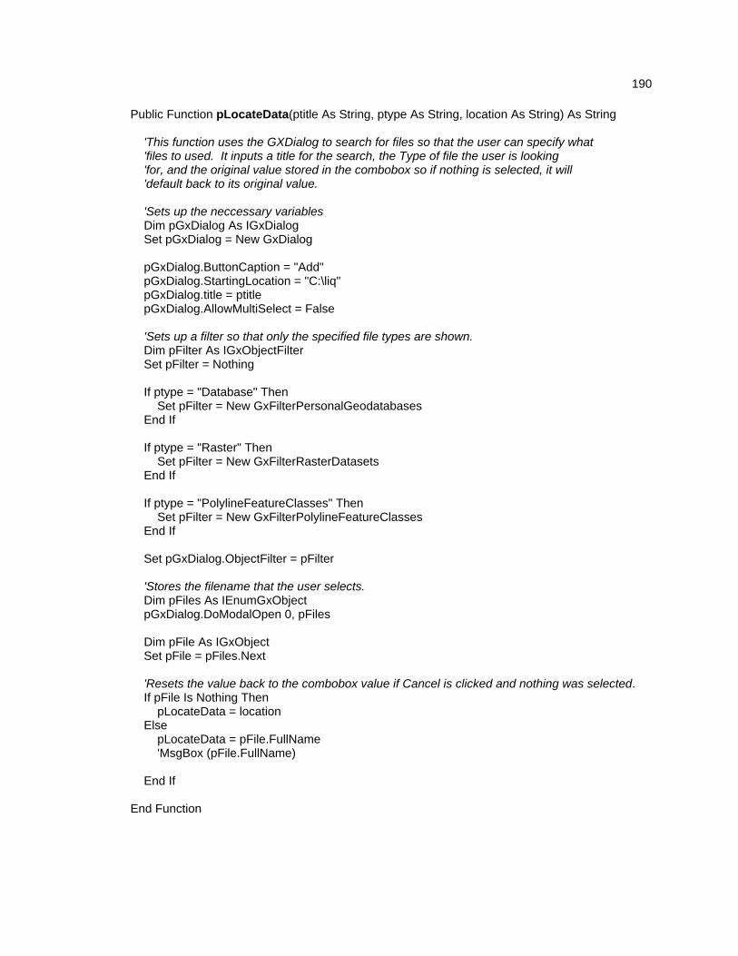
190

Public Function pLocateData(ptitle As String, ptype As String, location As String) As String 'This function uses the GXDialog to search for files so that the user can specify what 'files to used. It inputs a title for the search, the Type of file the user is looking 'for, and the original value stored in the combobox so if nothing is selected, it will 'default back to its original value. 'Sets up the neccessary variables Dim pGxDialog As IGxDialog Set pGxDialog = New GxDialog pGxDialog.ButtonCaption = "Add" pGxDialog.StartingLocation = "C:\liq" pGxDialog.title = ptitle pGxDialog.AllowMultiSelect = False 'Sets up a filter so that only the specified file types are shown. Dim pFilter As IGxObjectFilter Set pFilter = Nothing If ptype = "Database" Then Set pFilter = New GxFilterPersonalGeodatabases End If If ptype = "Raster" Then Set pFilter = New GxFilterRasterDatasets End If If ptype = "PolylineFeatureClasses" Then Set pFilter = New GxFilterPolylineFeatureClasses End If Set pGxDialog.ObjectFilter = pFilter 'Stores the filename that the user selects. Dim pFiles As IEnumGxObject pGxDialog.DoModalOpen 0, pFiles Dim pFile As IGxObject Set pFile = pFiles.Next 'Resets the value back to the combobox value if Cancel is clicked and nothing was selected. If pFile Is Nothing Then pLocateData = location Else pLocateData = pFile.FullName 'MsgBox (pFile.FullName) End If End Function

191

Public Function SiteAmplificationFactor(IBCSiteClass As String, pga As Double) As Double 'This function inputs the IBC Site Classification and the pga to 'determine the Site Amplification factor based on Seed et. al 2002 p. 42) ‘ Equations are approximate regression equations. Dim Soilgroundacceleration As Double If IBCSiteClass = "A" Then Soilgroundacceleration = 1 * pga ElseIf IBCSiteClass = "Ao" Then Soilgroundacceleration = 0.8086 * pga ElseIf IBCSiteClass = "AB" Then Soilgroundacceleration = -0.2698 * pga ^ 2 + 1.4655 * pga ElseIf IBCSiteClass = "B" Or IBCSiteClass = "C1" Or IBCSiteClass = "C2" Then If pga < 0.25 Then Soilgroundacceleration = -1.6119 * pga ^ 2 + 1.6311 * pga Else Soilgroundacceleration = -0.4985 * pga ^ 2 + 1.1398 * pga + 0.0538 End If ElseIf IBCSiteClass = "C4" Or IBCSiteClass = "D" Or IBCSiteClass = "E" Then If pga < 0.11 Or pga = 0.11 Then Soilgroundacceleration = -29.677 * pga ^ 2 + 4.5326 * pga ElseIf pga > 0.11 And pga > 0.45 Then Soilgroundacceleration = -0.9859 * pga ^ 2 + 1.1397 * pga + 0.1063 Else Soilgroundaccleration = -0.1022 * pga ^ 2 + 0.4506 * pga + 0.2399 End If End If SiteAmplificationFactor = Soilgroundacceleration If pga > 0.7 Then MsgBox ("Values are extrapolated above 0.7 g") End If End Function

APPENDIX D

DISK CONTENTS

193

This disk contains the data used for the Liquefaction/Lateral Spread hazard study done by Michael Olsen of the University of Utah for the Northern Salt Lake Valley. Questions about the data can be directed to Michael Olsen at michael.j.olsen@gmail.com.

The Analysis directory contains spreadsheets divided by geological units for histograms. The files beginning with Q are the ones that contain the histograms for soil types, blow counts, and Plastic Index. The other files are histograms for the hazard prediction within certain geological units. These are what appear in the thesis.

The Code directory contains exported modules (bas) and user forms (frm) for VBA that can be imported into ArcGIS for running the code.

The Database directory contains a processed and unprocessed version of the database used. It also includes various source files used to compile the database. Among those are various shear wave velocity calculations. I did the calculations for VS12m, but the VS30m were done by various other people. Due to time restraints, I did not clean up the files from what was given to me by the various sources. However, it shouldn’t take too long to find what you are looking for in those.

The Geology Mapping directory contains surficial geological data used for the project. The mapping is based on the mapping done by Personius and Scott (1992), Biek et al., 2004, and Miller (1980).

The LateralSpreadMap directory contains a geodatabase with the Lateral Spread hazard. It also contains a Shapefile of the Lateral Spread Hazard Map. It is in UTM NAD83 Z12N coordinates.

The liq directory contains the files used in the processing of the data and for the analysis. The DEMGridUTM is a DEM grid projected in UTM NAD 83 Zone 12 North for the study area. It is gridded at about a 9 m spacing. The slopegrid was created from this using ArcGIS spatial analyst. The Grdmot directory contains the Wong et al. (2002) map of peak ground accelerations gridded at a 30 m spacing. The GWgrid file is an interpolated groundwater grid (30 m spacing) based on the boreholes in the database. It was done using an inverse distance weighted method with ArcGIS spatial analyst. The utfaults and utrivers shapefiles were modified from those obtained by the AGRC. They show those portions used in the analysis only.

The maps directory contains the ArcGIS map files (mxd) which contain the code and display the information. The LiquefactionVBA91.mxd file contains the visual basic code for ArcGIS 9.1. The LiquefactionVBA83.mxd file contains the visual basic code for ArcGIS 8.3. The FinalLateralSpreadMap.mxd file contains the final GIS map.

The PGAdeaggregations contains bins of pga grided at 0.025 degree spacing for the Salt Lake Valley based as obtained from Steve Harmson at the USGS. For each grid point in each bin of pga, they contain values of M, R, and the probability of exceedance of that pga.

The River Depths directory contains HecRMS files of channel cross-sections used to obtain the river depths for the main channels in the Salt Lake Valley.

The SITEpdf directory contains the pdf files of the SPT boring logs that were input into the database.

The USGSQuads directory contains the topographic base maps by the USGS, as downloaded from the AGRC. They are in UTM NAD83 Z12 N projection.

194

REFERENCES Anderson, L.R., Keaton, J.R., Aubry, K., and Ellis, S.J., (1982). "Liquefaction potential map for Davis County, Utah", Final Report to the U.S. Geological Survey, January. Anderson, L.R., Keaton, J.R., and Bischoff, J.E., (1986b). "Liquefaction potential map for Utah County, Utah", Final Report to the U.S. Geological Survey", May. Anderson, L.R., Keaton, J.R., Bay, J.A., (1987). "Liquefaction potential map for the Northern Wasatch Front, Utah", Final Report to the U.S. Geological Survey". Anderson, L.R., Keaton, Rice, J.D., (1989). "Liquefaction potential map for Central Utah", Final Report to the U.S. Geological Survey". Anderson, L. R., Keaton, J. R., and Eldredge, S. N., (1994a). "Liquefaction-potential map for a part of Davis County, Utah: Utah Geological Survey Public Information Series 24, 1 sheet, 1:200,000. Anderson, L. R., Keaton, J. R., and Eldredge, S. N., (1994b). "Liquefaction-potential map for a part of Salt Lake County, Utah: Utah Geological Survey Public Information Series 24, 1 sheet, 1:300,000. Anderson, L. R., Keaton, J. R., and Eldredge, S. N., (1994c). "Liquefaction-potential map for a part of Utah County, Utah: Utah Geological Survey Public Information Series 24, 1 sheet, 1:365,000. Anderson, L. R., Keaton, J. R., and Eldredge, S. N., (1994c). "Liquefaction-potential map for a part of Weber County, Utah: Utah Geological Survey Public Information Series 24, 1 sheet, 1:200,000. Ashland, F., and Rollins, K. (1999). "Unpublished geotechnical and shear wave velocity database for the Salt Lake Valley”, Utah Geological Survey. Bartlett, S. F., and Youd T. L. (1992). "Empirical Analysis of Horizontal Ground Displacement Generated by Liquefaction-Induced Lateral Spreads," Technical Report NCEER-92-0021, National Center for Earthquake Engineering Research, Buffalo, NY, August 17. Bartlett, S.F., and Youd, T.L. (1995). “Empirical prediction of liquefaction-induced lateral spread.” J. Geotech Engrg., ASCE, Vol. 121, No. 4, April, pp. 316-329. Biek, R.F., Solomon, B.J., Keith, J.D., and Smith, T.W., (2004). Interim geologic maps of the Copperton, Magna, and Tickville Spring quadrangles, Salt Lake and Utah Counties, Utah: Utah Geological Survey Open-File Report 434, scale 1:24,000. Bischoff, T.A., 2005, “Collection of shear wave velocity data for use in Utah Geological Survey Site-Conditions maps and database,” Master’s Project, Utah State University Boulanger, R. W., and Idriss, I.M., (2004). "Evaluating the Potential for Liquefaction or Cyclic Failure of Silts and Clays," Technical Report UCD/CGM-04/01, Center for Geotechnical Modeling Currey, D.R., and Oviatt, C.G., (1985). “Durations, average rates, and probable causes of Lake Bonneville expansions, still-stands, and contractions during the last deep-lake cycle, 32,000–10,000 years ago: in Kay, P.A., and Diaz, H.F., eds.”, Problems of and prospects for predicting Great Salt Lake levels: Papers from a conference held in Salt Lake City, March 26–28, 1985: Center for Public Affairs and Administration, University of Utah, p. 9-24.

195

Dames and Moore, (1996a). "Geotechnical Report for the Reconstruction of Structures and Embankments 600 South Section I-15 Corridor From 600 South to 960 South," UDOT Contract No. SP-15-7(129)310, Station 31+275 to 32+420, Salt Lake City, Utah, Sept. 1996. Dames and Moore, (1996b). "Geotechnical Report for the Reconstruction of Structures and Embankments 1300 South Section I-15 Corridor," UDOT Contract No. SP-15-7(132)308, Station 29+300 to 31+275, Salt Lake City, Utah, Sept. 1996. Dames and Moore, (1996c). "Geotechnical Report for the Reconstruction of Structures and Embankments 2400 South Section I-15 Corridor," UDOT Contract No. SP-15-7(1287308, Station 26+800 to 29+300, Salt Lake City, Utah, Sept. 1996. Davis, F.D., (1983). Geologic map of the central Wasatch Front, Utah: Utah Geological and Mineral Survey Map 54-A, scale 1:100,000. DeLisle, M.J., (2000). “Liquefaction Zones in the City and County of San Francisco, California,” Sesimic Hazard Evaluation of the City and County of San Francisco, California, California Division of Mines and Geology Open File Report 2000-009, pp. 2-15. FEMA (1999). Federal Emergency Management Agency, "HAZUS 99 Technical Manual," Vol. 1. Frankel, A., Mueller, C., Barnhard, T., Perkins, D., Leyendecker, E. V., Dickman, N., Hanson, S., and Hopper, M. (1996). "National Seismic-Hazards Maps: Documentation, June 1996, U.S.G.S. Open-File Report 96-532. International Building Code (2000). International Code Council, Inc., 2000, International Building Code, Building Officials and Code Administrators International, Inc., Country Club Hills, IL; International Conference of Building Officials, Whittier, CA; and Southern Building Code Congress International, Inc., Birmingham, AL. Keaton, J. R., and Anderson, L. R. (1995). "Mapping Liquefaction Hazards in the Wasatch Front Region: Opportunities and Limitations," Environmental and Engineering Geology of the Wasatch Front Region, Utah Geological Association Publication, 24, 1995. Kleindfelder, Inc. (1996a). "Preliminary Geotechnical Exploration Report," I-15 Corridor Reconstruction Section 4, 600 South, Project No. SP-15-7(129)310, Station 32+080 to 35+044, Salt Lake City, Utah, Sept. 1996. Kleindfelder, Inc. (1996b). "Geotechnical Exploration Report," I-15 Corridor Reconstruction Section 9, State Street, Project No. SP-80-3(41)125, Station 1+220 to 1+687, Salt Lake City, Utah, Sept. 1996. Kleindfelder, Inc. (1996c). "Geotechnical Exploration Report," I-15 Corridor Reconstruction Section 8, 3300 South, Project No. SP-15-7(144)305, Station 28+600 to 24+500, Salt Lake City, Utah, Sept. 1996. Kleindfelder, Inc. (1996d). "Geotechnical Exploration Report," I-15 Corridor Reconstruction Section 10, 900 W., Project No. SP-020(1)17, Station 1+000 to 10+640, Salt Lake City, Utah, Sept. 1996. Kleindfelder, Inc. (1999). "Geotechnical Investigation MHJ Block 37," City Library, Parking Structure and Physical Plant, Southeast corner 400 South and 200 East Salt Lake City, Utah, Project No. 35-8018-25.001, Aug. 1999.

196

Kramer, S. L., 1996, Geotechnical Earthquake Engineering, Prentice Hall, Upper Saddle River, New Jersey, Chapter 4. Liao, S. S. C., Veneziano, D., and Whitman, R. V. (1988). "Regression models for evaluating liquefaction probability," Journal of Geotechnical Engineering, ASCE, Vol. 112, No. 1, pp. 44-59. Marrone, J., Ostadan, F., Youngs, R., Litehiser, J., (2003). “Probabilistic Liquefaction Hazard Evaluation: Methods and Applications,” Transactions of the 17th International Conference on Structural Mechanics in Reactor Technology (SMiRT 17), Prague, Czech Republic, August 17-22, 2003, Paper # M02-1. Miller, R.D., (1980). Surficial geologic map along part of the Wasatch Front, Salt Lake Valley, Utah: U.S. Geological Survey Miscellaneous Field Studies Map MF-1198, scale 1:100,000. NCEER (1997). "Proceedings of the NCEER Workshop on Evaluation of Liquefaction Resistance of Soils," edited by Youd, T. L., and Idriss, I. M., Technical Report NCEER-97-0022, National Center for Earthquake Engineering Research. NEHRP (1997). "NEHRP Recommend Provisions for Seismic Regulations for New Buildings and Other Structures," 1997 Edition Part 1: Provisions (FEMA 302), prepared by the Building Seismic Safety Council for the Federal Emergency Management Agency, Washington, D.C. O’Rourke, T.D., and Pease, J.W. (1992). “Mapping liquefiable layer thickness for seismic hazard assessment.” Journal of Geotechnical and Geoenvironmental Engineering, ASCE, Vol. 123, No. 1, January, pp. 46-56. Ostadan, F., Marrone, J., Litehiser, J. and Arango, I, (1991) “Liquefaction Hazard Evaluation: Methodology and Application,” Lifeline Earthquake Engineering, Monograhph No. 4, pp. 591-600. Personius, S.F., and Scott, W.E., (1992). Surficial geologic map of the Salt Lake City segment and parts of adjacent segments of the Wasatch fault zone, Davis, Salt Lake, and Utah Counties, Utah: U.S. Geological Survey Miscellaneous Investigations Map I-2106, scale 1:50,000. Power, M.S., and Holzer, T.L., (1996). “Liquefaction Maps,” Applied Technical Council, ATC -35 Technical Brief, http://www.atcouncil.org/pdfs/atc-35.pdf Rosinski, A., Knudsen, K.L., Wu, J., Seed, R.B., Real, C.R., (2004). "Development of Regional Liquefaction-Induced Deformation Hazard Maps," GeoTrans 2004, Geotechnical Engineering for Transportation Projects (GSP No. 126), ASCE Conf. Proc. Vol. 154, No. 67, pp. 797-806 Seed, R. B., Cetin, K. O., Moss, R. E. S., Kammerer, A. M., Wu, J., Petana, J. M., Riemer, M. F. (2001). "Recent Advances in Soil Liquefaction Engineering and Seismic Site Response Evaluation," Fourth International Conference on Recent Advances in Geotechnical Earthquake Engineering and Soil Dynamics, University of Missouri-Rolla, Rolla, Missouri, 2001, 45 pages, Paper No. SPL-2. Solomon, B.J., Storey, N.S., Wong, I., Silva, W., Gregor, N., Wright, D., McDonald, G., (2004). "Earthquake-Hazards Scenario for a M7 Earthquake on the Salt Lake City Segment of the Wasatch Fault Zone," Utah Geological Survey, Special Study 111DM. Tooker, E.W., and Roberts, R.J., (1971). Geologic map of the Garfield quadrangle, Salt Lake and Tooele Counties, Utah: U.S. Geological Survey Geologic Quadrangle Map GQ-922, scale 1:24,000.

197

Tooker, E.W., and Roberts, R.J., (1971). Geologic map of the Magna quadrangle, Salt Lake County, Utah: U.S. Geological Survey Geologic Quadrangle Map GQ-923, scale 1:24,000. Toprak, S., and Holzer, T.L., (2003). "Liquefaction Potential Index: Field Assessment," Journal of Geotechnical and Environmental Engineering, Vol. 129, No. 4, April 2003, pp. 315-322. Wong, I., Silva, W., Wright, D., Olig, S., Ashland, F., Gregor, N., Christenson, G., Pechmann, J., Thomas, P., Dober, M., Gerth, R., (2002). Ground-Shaking Map for a Magnitude 7.0 Earthquake on the Wasatch Fault, Salt Lake City, Utah, Metropolitan Area, Utah Geological Survey Public Information Series 76, Utah Geological Survey Miscellaneous Publication MP 02-05 Youd, T. L., and Perkins, D. M. (1978). "Mapping Liquefaction-Induced Ground Failure Potential," Journal of the Geotechnical Engineering Division, ASCE, Vol. 104, No. GT4, Proc Paper 13659, April, 1978, pp. 433-446. Youd, T.L., and Perkins, D.M., (1987). “Mapping of Liquefaction Severity Index,” Journal of Geotechnical Engineering Division, American Society of Civil Engineers, v. 118, p. 1374-1392. Youd, T.L., Idriss, I.M. Andrus, R.D. Arango, I., Castro, G., Christian, J.T., Dobry, R., Liam Finn, W.D.L., Harder, L.F., Jr., Hynes, M.E., Ishihara, K., Koester, J.P., Liao, S.S.C., Marcuson, W.F., III, Martin, G.R., Mitchell, J.K., Moriwaki, Y., Power, M.S., Robertson, P.K., Seed, R.B., Stokoe, K.H., II (2001). “Liquefaction resistance of soils: Summary Report from the 1996 NCEER and 1998 NCEER/NSF Workshops on Evaluation of Liquefaction Resistance of Soils”, Journal of Geotechnical and Environmental Engineering, Vol. 127, No. 10, Oct. 2001, pp. 817-833. Youd, T.L., Hansen, C.M., Bartlett S.F., (2002). "Revised Multilinear Regression Equations for Prediction of Lateral Spread Displacement," Journal of Geotechnical and Environmental Engineering, December 2002, pp. 1007-1017.