automatic differentiation methods in computational ...alex/ima/ima1.pdf · automatic...
TRANSCRIPT

Preface Functional equations in DS AD and multivariate power series Parameterizations of invariant manifolds An elementary example Conclusions
Automatic Differentiation methods incomputational Dynamical Systems: invariant
manifolds and normal forms
Àlex Haro
Departament de Matemàtica Aplicada i AnàlisiUniversitat de Barcelona
IMA (University of Minnesota), June 2011

Preface Functional equations in DS AD and multivariate power series Parameterizations of invariant manifolds An elementary example Conclusions
PrefacePoincaré’s program
Poincaré’s program for global analysis of dynamical systems (DS):
Identify equilibriums and periodic orbits.Identify the invariant manifolds associated to them.Identify other invariant manifolds (e.g. invariant tori).
The long term behaviour of a dynamical system is organized by itsinvariant objects.
These objects constitute the skeleton of the DS.
Nowadays: The qualitative approach can be made very quantitative!

Preface Functional equations in DS AD and multivariate power series Parameterizations of invariant manifolds An elementary example Conclusions
Preface 3My (and your!) goals of the lectures
Describe a unified framework for the computation of invariantmanifolds and normal forms attached to fixed points of vectorfields using power series.
Adapt the methodology to elementary models. By elementary wemean that the model can be written using arithmetic operationsand elementary functions.
Introduce methods of Automatic Differentiation.Estimate complexities.
Apply the methodology to a concrete example: center manifoldsof Lagrange equilibrium points in the Restricted Three BodyProblem.

Preface Functional equations in DS AD and multivariate power series Parameterizations of invariant manifolds An elementary example Conclusions
Preface 4Sources of inspiration
Poincaré, Arnold, ...
C. Simó, “On the Analytical and Numerical Approximation ofInvariant Manifolds” (1990)X. Cabré, E. Fontich, R. de la Llave, “The parameterizationmethod for invariant manifolds” (2003)À. Jorba,“A methodology for the numerical computation ofnormal forms, centre manifolds and first integrals of Hamiltoniansystems” (1999)
D. E. Knuth, “The art of computer programming. Vol. 2:Seminumerical algorithms” (3rd rev., 1997)
Notes of the course:http://www.ima.umn.edu/2010-2011/ND6.20-7.1.11/abstracts.html#11183

Preface Functional equations in DS AD and multivariate power series Parameterizations of invariant manifolds An elementary example Conclusions
Table of contents
1 Functional equations in Dynamical Systems
2 Automatic Differentiation and multivariate power series
3 Parameterizations of invariant manifolds
4 An elementary example
5 Conclusions

Preface Functional equations in DS AD and multivariate power series Parameterizations of invariant manifolds An elementary example Conclusions
Functional equations inDynamical Systems

Preface Functional equations in DS AD and multivariate power series Parameterizations of invariant manifolds An elementary example Conclusions
Functional Equations in Dynamical Systems 7Some examples and methodologies
Examples:The solution of odesThe normal form equationsThe invariance equations for invariant manifolds
Methodologies:Expand the unknowns using series (Taylor, Fourier,Fourier-Taylor), approximate them using interpolants(polynomials, splines, etc.)Solve the equations “order by order” (on-line methods for powerseries)Solve the equations using e.g. Newton method
Remark:We have to evaluate the dynamical system on the series!
These tasks depend a lot on the problem.

Preface Functional equations in DS AD and multivariate power series Parameterizations of invariant manifolds An elementary example Conclusions
Invariant manifolds for maps 8Setting the equations
Given:a map in Rn:
z = F (z)
a d-manifoldW, parameterized by
z = W (s),
where W : U ⊂ Rd →W ⊂ Rn
a map inW, written in coordinates on U ⊂ Rd as
s = f (s)
then:The manifoldW parameterized by W is invariant under F ,with subsystem given by f , if
F (W (s)) = W (f (s)) .

Preface Functional equations in DS AD and multivariate power series Parameterizations of invariant manifolds An elementary example Conclusions
Invariant manifolds for maps 9Setting the equations

Preface Functional equations in DS AD and multivariate power series Parameterizations of invariant manifolds An elementary example Conclusions
Pictures at an exhibition 10Stable and unstable manifolds in a 4D economic growth model
R(1,1),t+1 =1
1 + α− αR(2,1),t
R(2,2),t+1 =1
1 + β − βR(1,2),t
R(1,2),t+1 = R(2,2),t+1 ·R(2,2),t
R(2,1),t
R(2,1),t+1 = R(1,1),t+1 ·R(1,1),t
R(1,2),t
(with Pere Gomis-Porqueras)

Preface Functional equations in DS AD and multivariate power series Parameterizations of invariant manifolds An elementary example Conclusions
Pictures at an exhibition 11Stable and unstable manifolds of a 2-period torus in a qp driven system
x = x + y mod 1
y = y −sin(2πx)
2π(κ + λ cos(2πθ))
θ = θ + ω mod 1
with R. de la Llave

Preface Functional equations in DS AD and multivariate power series Parameterizations of invariant manifolds An elementary example Conclusions
Pictures at an exhibition 12Meandering KAM tori in a degenerate area preserving map
8><>:x = x + (y + 0.1)(y − 0.2) ,
y = y −κ
2πsin(2πx) .
-0.4
-0.3
-0.2
-0.1
0
0.1
0.2
0.3
0.4
0.5
0 0.1 0.2 0.3 0.4 0.5 0.6 0.7 0.8 0.9 1
y
x
K= 0.430396
with R. de la Llave and A. González

Preface Functional equations in DS AD and multivariate power series Parameterizations of invariant manifolds An elementary example Conclusions
Pictures at an exhibition 13Normally hyperbolic tori in a non-conservative system
0 1
2 3
4 5
6 -0.5-0.4
-0.3-0.2
-0.1 0
0.1 0.2
0.3 0.4
0.5
-2.5-2
-1.5-1
-0.5 0
0.5 1
1.5 2
2.5
z
xy
z
0
1
2
3
4
5
6
0 1 2 3 4 5 6
f
x
Invariant torus and dynamics in the fattened Arnold family:
x = x + a + ε(y +z2
+ sin x)
y = b(y + sin x)
z = c(y + z + sin x)
with a = 0.1, b = 0.3, c = 2.4, ε ' 0.750396. (with Marta Canadell)

Preface Functional equations in DS AD and multivariate power series Parameterizations of invariant manifolds An elementary example Conclusions
Pictures at an exhibition 14Computer assisted proofs on the verge of a hyperbolicity breakdown
Invariant tori and normal dynamics of a 2 period torus of the qp driven logistic map
z = a(1 + D cos(2πθ))z(1− z)
θ = θ + ω,
where ω =√
5−12 , and a and D are parameters. (with Jordi-Lluís Figueras)
Preface Functional equations in DS AD and multivariate power series Parameterizations of invariant manifolds An elementary example Conclusions
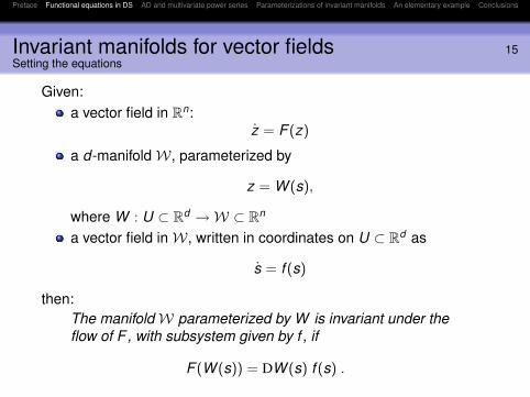
Invariant manifolds for vector fields 15Setting the equations
Given:a vector field in Rn:
z = F (z)
a d-manifoldW, parameterized by
z = W (s),
where W : U ⊂ Rd →W ⊂ Rn
a vector field inW, written in coordinates on U ⊂ Rd as
s = f (s)
then:The manifoldW parameterized by W is invariant under theflow of F , with subsystem given by f , if
F (W (s)) = DW (s) f (s) .

Preface Functional equations in DS AD and multivariate power series Parameterizations of invariant manifolds An elementary example Conclusions
Functional equations 16Unknowns
In the invariance equation:There is a known term, F .There are two unknowns, W and f .
The system is underdetermined:There are n equations.There are n + d unknown d-variate functions.

Preface Functional equations in DS AD and multivariate power series Parameterizations of invariant manifolds An elementary example Conclusions
Functional equations 17Particular setting
Setting the problem
Given a fixed point z0, with a d-dimensional invariant subspace forthe linearization z = DF (z0)z around z0, associate an invariantmanifold tangent to such subspace.
Semi-local analysis. We will expand the manifold (and its dynamics)using power (or Taylor) series.
Globalization. The semi-local analysis is the first step to globalizethe manifold, that is to extend the manifold far away of the fixed point.
1D stable/unstable manifolds is straigtforward.2D stable/unstable manifolds, see [KrauskopfODHGVDJ05].High order approximations are crucial for center manifolds.

Preface Functional equations in DS AD and multivariate power series Parameterizations of invariant manifolds An elementary example Conclusions
Functional equations 18Composition with the system
Important fact
The term F (W (s)) involves compositions of the system with theparameterization.
Many times the model F is elementary, and the compositions can bemade very efficiently!

Preface Functional equations in DS AD and multivariate power series Parameterizations of invariant manifolds An elementary example Conclusions
Automatic Differentiation andMultivariate power series

Preface Functional equations in DS AD and multivariate power series Parameterizations of invariant manifolds An elementary example Conclusions
Algebraic Manipulation 20Series as algebraic objects
Observation: series are algebraic objects.
Algebraic Manipulation
AM is a set of techniques based on the mechanical application ofalgebraic operations on series, such as arithmetic operations andcompositions.
Some AM C/C++ sofware: TRIP, Piranha.
This approach has a long story in Celestial Mechanics!
Preface Functional equations in DS AD and multivariate power series Parameterizations of invariant manifolds An elementary example Conclusions
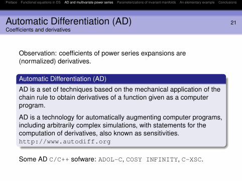
Automatic Differentiation (AD) 21Coefficients and derivatives
Observation: coefficients of power series expansions are(normalized) derivatives.
Automatic Differentiation (AD)
AD is a set of techniques based on the mechanical application of thechain rule to obtain derivatives of a function given as a computerprogram.
AD is a technology for automatically augmenting computer programs,including arbitrarily complex simulations, with statements for thecomputation of derivatives, also known as sensitivities.http://www.autodiff.org
Some AD C/C++ sofware: ADOL-C, COSY INFINITY, C-XSC.

Preface Functional equations in DS AD and multivariate power series Parameterizations of invariant manifolds An elementary example Conclusions
Automatic Differentiation and Algebraic Manipulation 22Merging the two technologies
Derivatives of arithmetic operations of power series can be performedeasily from the corresponding algebraic operations.
Derivatives of composition of power series with elementary functionscan be performed on-line (order by order), à la Knuth.

Preface Functional equations in DS AD and multivariate power series Parameterizations of invariant manifolds An elementary example Conclusions
Multivariate power series 23Definitions and notations
DefinitionGiven a commutative ring K (like K = R or K = C), a (formal) powerseries in the variables x = (x1, . . . , xd ) with coefficients in K is anelement of the ring K[[x ]] = K[[x1, . . . , xd ]],
f (x) =∞∑
k=0
fk (x) , (1)
where each fk (x) is a homogeneous polynomial of order k , that is anelement of Kk [x ], which we write
fk (x) =∑
m1+···+md =k
fm1,...,md xm11 . . . xmd
d =∑|m|=k
fmxm
We also denote the k th truncation as f≤k (x) =k∑
i=0
fi (x).

Preface Functional equations in DS AD and multivariate power series Parameterizations of invariant manifolds An elementary example Conclusions
Multivariate power series 24Homogeneous polynomials
Recursive scheme
A homogeneous polynomial fk (x) of d variables x = (x1, . . . , xd ) oforder k is a combination of (k + 1) homogeneous polynomials of thefirst (d − 1) variables x = (x1, . . . , xd−1) of degrees k , k − 1, . . . ,0:
fk (x) = f dk (x) + f d
k−1(x)xd + · · ·+ f d0 (x)xk
d .
A k th order homogeneous polynomial is represented as:
A vector of hd (k) :=(d+k−1
d−1
)coefficients, in graded reverse
lexicographic ordering w.r.t. the keys m = (m1,m2, . . . ,md ).
A recursive tree.
A k th truncated power series has nd (k) :=(d+k
d
)coefficients.

Preface Functional equations in DS AD and multivariate power series Parameterizations of invariant manifolds An elementary example Conclusions
Some implementation details 25Storage of coefficients
Two main approaches
For dense power series, one stores all the coefficients.
For sparse power series, one stores the non-zero terms,corresponding to coefficient-key pairs.
Here: dense polynomials, without structure.
TRIP and Piranha supports sparse series.

Preface Functional equations in DS AD and multivariate power series Parameterizations of invariant manifolds An elementary example Conclusions
Some implementation details 26Graded reverse lexicographical ordering
Observation: The ordering of the coefficients is induced by therecursive tree scheme.
Example
The 10 coefficients of a homogenous 3-variate polynomial of order 3are ordered following the scheme:
x31 , x
21 x2, x1x2
2 , x32 , x
21 x3, x1x2x3, x2
2 x3, x1x23 , x2x2
3 , x33 .

Preface Functional equations in DS AD and multivariate power series Parameterizations of invariant manifolds An elementary example Conclusions
Some implementation details 27Data structures
1 / / s t r u c t u r e f o r homogeneous terms2 / / the c o e f f i c i e n t s are double type34 struct homog5 {6 unsigned char nv , orden ; / / number o f va r iab les , homogeneous order7 double ∗coef ; / / address o f the f i r s t c o e f f i c i e n t8 struct homog ∗ term ; / / f o r t r ee d i s t r i b u t i o n o f c o e f f i c i e n t s9 } ;
1011 typedef struct homog homog ;1213 / / s t r u c t u r e f o r power se r i es1415 typedef struct16 {17 unsigned char nv , orden ; / / number o f va r iab les , order o f the se r i es18 homog ∗∗ term ; / / l i s t o f homogeneous terms19 }20 se r i e ;

Preface Functional equations in DS AD and multivariate power series Parameterizations of invariant manifolds An elementary example Conclusions
Product of (truncated) power series 28Schoolbook formula
The key routine, on which the rest of routines are built, is the(truncated) product of power series, that reduces to perform productsof homogeneous polynomials.
We use the naive convolution formula, whose cost (number ofoperations) is
pd (k) =
(2d + k
2d
)∼ 1
(2d)!k2d ∼ d !2
(2d)!nd (k)2 .
By operation we mean "one multiplication of coefficients, oneaddition, and index the result".
Important:The method is on-line.Easy to implement.

Preface Functional equations in DS AD and multivariate power series Parameterizations of invariant manifolds An elementary example Conclusions
Product of (truncated) power series 29Fast methods
There are (asymptotically) fast convolution algorithmsKaratsuba and Toom-Cook methods, with cost ∼ nα, with α < 2,n = nd (k).FFT methods, with multi-evaluation and interpolation techniquesand reduction to univariate series, with cost ∼ n log(n), withn = nd (k).
Important:useful only for very high order (not usual in DS).multi-evaluation and interpolation produces numerical errors.

Preface Functional equations in DS AD and multivariate power series Parameterizations of invariant manifolds An elementary example Conclusions
Some implementation details 30Scalar multiplication of a homogenous polynomial
Natural code
1 void smulth (homog ∗h , double r , homog ∗a )2 {3 unsigned i n t m, nch ;45 nch= nch ( h−>nv , h−>orden ) ;67 for (m= 0; m<nch ; m++){8 h−>coef [m]+= r∗ a−>coef [m] ;9 }
10 }
Fancy code
1 void smulth (homog ∗h , double r , homog ∗a )2 {3 double ∗hc , ∗hf , ∗ac ;45 hf= h−>coef + nch ( h−>nv , h−>orden ) ;6 for ( hc= h−>coef , ac= a−>coef ; hc<hf ; (∗hc)+= r∗ (∗ac ) , hc++ , ac ++) ;7 }

Preface Functional equations in DS AD and multivariate power series Parameterizations of invariant manifolds An elementary example Conclusions
Some implementation details 31Product of homogeneous polynomials
1 void sprodh (homog ∗p , homog ∗a , homog ∗b )2 {3 i f ( p−>nv >2) {4 i f ( a−>orden ) {5 i f ( b−>orden ) {6 homog ∗aa , ∗bb , ∗pp , ∗pp0 , ∗af , ∗bf ;7 a f= a−>term+a−>orden ; b f= b−>term+b−>orden ;8 for ( aa= a−>term , pp0= p−>term ; aa<af ; aa++ , pp0++) {9 for ( bb= b−>term , pp= pp0 ; bb<bf ; sprodh ( pp , aa , bb ) , bb++ , pp ++) ;
10 smulth ( pp , ∗(bb−>coef ) , aa ) ;11 }12 for ( bb= b−>term , pp= pp0 ; bb< bf ; smulth ( pp , ∗(aa−>coef ) , bb ) , bb++ , pp ++) ;13 ∗(pp−>coef )+= ∗(aa−>coef ) ∗ ∗(bb−>coef ) ;14 }15 else smulth ( p , ∗(b−>coef ) , a ) ;16 }17 else smulth ( p , ∗(a−>coef ) , b ) ;18 }19 else i f ( p−>nv == 2) { / / 2−v a r i a t e polynomia ls20 double ∗aa , ∗bb , ∗pp , ∗pp0 , ∗af , ∗bf ;21 a f= a−>coef+a−>orden ; b f= b−>coef+b−>orden ;22 for ( aa= a−>coef , pp0= p−>coef ; aa<= af ; aa++ , pp0++)23 for ( bb= b−>coef , pp= pp0 ; bb<= bf ; ∗pp+= ∗aa ∗ ∗bb , bb++ , pp ++) ;24 }25 else ∗(p−>coef )+= ∗(a−>coef ) ∗ ∗(b−>coef ) ; / / 1−v a r i a t e polynomia ls26 }

Preface Functional equations in DS AD and multivariate power series Parameterizations of invariant manifolds An elementary example Conclusions
Benchmarks 32Estimating the overhead
An efficient implementation of the (truncated) product of power seriesis based on an efficient indexation of the coefficients.
We define the overhead as the ratio of the execution time ofcomputing the (k th truncated) product over the execution time ofcomputing pd(k) products and additions.
1 for ( i = 0 ; i <= k ; i ++) {2 for ( j = 0 ; j <= i ; j ++) {3 n i f = nch ( n , i−j ) ;4 n j f = nch ( n , j ) ;5 for ( n i = 0 ; n i < n i f ; n i ++) {6 for ( n j = 0 ; n j < n j f ; n j ++) {7 z+= x∗y ;8 }9 }
10 }11 }

Preface Functional equations in DS AD and multivariate power series Parameterizations of invariant manifolds An elementary example Conclusions
Benchmarks 33Comparison of several implementations
d = 4 tree TRIP ad hock n p time (s) Mflops over. time (s) time (s)
10 1001 43758 2.930e – 04 149.3 3.05 NA 3.665e – 0420 10626 3108105 1.364e – 02 227.9 2.50 NA 1.906e – 0230 46376 48903492 1.900e – 01 257.4 2.38 2.000e – 01 2.529e – 0140 135751 377348994 1.120e+00 336.9 1.70 1.630e+00 1.767e+0050 316251 1916797311 5.050e+00 379.6 1.53 7.660e+00 1.032e+0160 635376 7392009768 1.793e+01 412.3 1.42 2.928e+01 5.371e+0170 1150626 23446881315 5.335e+01 439.5 1.34 9.257e+01 2.098e+0280 1929501 64276915527 1.393e+02 461.5 1.27 2.533e+02 6.623e+0290 3049501 157366449604 3.282e+02 479.5 1.23 6.229e+02 1.765e+03
100 4598126 352025629371 7.093e+02 496.3 1.19 1.408e+03 4.195e+03
d = 6 tree TRIP ad hock n p time (s) Mflops over. time (s) time (s)
10 8008 646646 4.808e – 03 134.5 4.17 NA 4.451e – 0220 230230 225792840 1.310e+00 172.4 3.36 9.940e – 01 1.722e+0130 1947792 11058116888 5.043e+01 219.3 2.69 4.408e+01 9.161e+0240 9366819 206379406870 7.808e+02 264.3 2.23 8.367e+02 1.926e+0450 32468436 2160153123141 7.183e+03 300.7 1.96 NA NA

Preface Functional equations in DS AD and multivariate power series Parameterizations of invariant manifolds An elementary example Conclusions
Benchmarks 34log-log plot of executions times
1e-08
1e-06
1e-04
1e-02
1e+00
1e+02
1e+04
1e+06
1e+01 1e+02 1e+03 1e+04 1e+05 1e+06 1e+07 1e+08
t
n
d= 3: a= -8.59, b= 1.72d= 4: a= -8.79, b= 1.73d= 5: a= -8.93, b= 1.73d= 6: a= -8.95, b= 1.70
Fit t(n) ' A nb, where a = log10 A
Time is subquadratic in n (or sublinear in p)!

Preface Functional equations in DS AD and multivariate power series Parameterizations of invariant manifolds An elementary example Conclusions
Benchmarks 35Dependencies
The algorithm: we use the naive formula, which involves pd (k)products and additions of numbers. We take advantage of thetree data structure, and use recursivity.The implementation: we use the programming language C.The computer: iMac running under Mac OS X 10.6.4. Technicalspecifications: 2 GHz Intel Core Due, 4MB L2 Cache; Memory: 1GB 667 MHz DDR2 SDRAM.The coefficients: these are real numbers in double-precisionfloating-point arithmetic, the variable type double in C (8 bytesper coefficient).The compiler: we use gcc with different options and flags.The plug: time execution can vary a lot if the laptop is notplugged in and work with the battery.
The list does not finish here.

Preface Functional equations in DS AD and multivariate power series Parameterizations of invariant manifolds An elementary example Conclusions
Benchmarks 36Efficient implementation
Efficient implementation!
The Mathematica implementation of an FFT method take hours tocompute the truncated exponential up to order 10 of a 10-variatepower series on a PC [Neidinger05].
Our C implementation of the NAIVE algorithm take less than 0.20seconds on a slightly old laptop.

Preface Functional equations in DS AD and multivariate power series Parameterizations of invariant manifolds An elementary example Conclusions
Composition with elementary functions 37Make AD work!
Composition of formal power series is a very hard task, but in specialcases (e.g. composing with elementary functions), the cost isproportional to that of the product!
Problem: Compute ϕ ◦ f (x), where ϕ is an elementary function(solution of a simple ode), and f is a power series.
Very well-known formulas for 1-variate power series (Knuth).
Formulas for multivariate power series?Reduction to 1-variate case (not on-line!).Use chain rule ∇(ϕ ◦ f )(x) = ϕ′(f (x))∇f (x) [Neidinger 95,10][Barrio 06]

Preface Functional equations in DS AD and multivariate power series Parameterizations of invariant manifolds An elementary example Conclusions
Composition with elementary functions 38Radial derivative
The radial derivative of a function (power series) f (x) =∞∑
k=0
fk (x) is
defined by
Rf (x) = Df (x) x =∞∑
k=0
k · fk (x) .
Euler Identity
For a k th order homogeneous function, fk : Rfk (x) = k · fk (x) .
Chain rule
For an univariate function ϕ = ϕ(t) and a multivariate functionf = f (x):
R(ϕ◦f )(x) = ϕ′(f (x)) Rf (x) .

Preface Functional equations in DS AD and multivariate power series Parameterizations of invariant manifolds An elementary example Conclusions
Composition with elementary functions 39Applications to AD
Key observation in AD. If ϕ satisfies an elementary differentialequation, then we can compute ϕ◦f on-line à la Knuth.
Example
If ϕ(t) = et , then e(x) = exp(f (x)) satisfies Re(x) = e(x)Rf (x).Since e0 = exp(f0), the series e(x) is computed recursively by
ek (x) =1k
k−1∑j=0
(k − j)fk−j (x)ej (x) .
Notice that the cost up to order k is ∼ pd (k).

Preface Functional equations in DS AD and multivariate power series Parameterizations of invariant manifolds An elementary example Conclusions
Example
The series p(x) = (f (x))α can be computed recursively from p0 = fα0by
pk (x) =1
k f0
k−1∑j=0
(α(k − j)− j) fk−j (x)pj (x) .
Notice that the cost up to order k is ∼ pd (k).
Same tricks are applied to many others elementary functions, and theresulting algorithms have a cost that is proportional to the cost of aproduct. See the notes!

Preface Functional equations in DS AD and multivariate power series Parameterizations of invariant manifolds An elementary example Conclusions
Comparing codes 41C-XSC implementation of power function of exponent α, for 2-variate power series
1 l d i m 2 t a y l o r power ( const l d i m 2 t a y l o r& s , const l _ i n t e r v a l & alpha )2 {3 l d i m 2 t a y l o r erg ( s . p ) ;4 i d o t p r e c i s i o n sum_idot ;5 l _ i n t e r v a l sum1 , sum2 , h ;67 erg [ 0 ] [ 0 ] = pow( s [ 0 ] [ 0 ] , alpha ) ;8 for ( i n t j =1; j <=erg . p ; j ++) {9 sum_idot= i n t e r v a l ( 0 . 0 ) ;
10 for ( i n t i =0; i <= j−1; i ++) {11 h=alpha∗( i n t e r v a l ( j )− i n t e r v a l ( i ))− i n t e r v a l ( i ) ;12 accumulate ( sum_idot , h∗erg [ 0 ] [ i ] , s [ 0 ] [ j−i ] ) ;13 }14 sum1 = l _ i n t e r v a l ( sum_idot ) ;15 erg [ 0 ] [ j ]=sum1 / i n t e r v a l ( j ) / s [ 0 ] [ 0 ] ;16 }17 for ( i n t i =1; i <=erg . p ; i ++) { / / remaining erg ( i , k )18 for ( i n t k =0; k<=erg . p−i ; k++) {19 sum_idot= i n t e r v a l ( 0 . 0 ) ;20 for ( i n t l =0; l <= i−1; l ++) { / / Do not sum coe f f . ( l ,m)= (0 ,0 )21 h=alpha∗( _ i n t e r v a l ( i )−_ i n t e r v a l ( l ))− _ i n t e r v a l ( l ) ;22 for ( i n t m=0; m<=k ; m++) {23 accumulate ( sum_idot , h∗erg [ l ] [m] , s [ i−l ] [ k−m] ) ;24 }25 }26 sum1 = l _ i n t e r v a l ( sum_idot ) ;27 sum_idot= i n t e r v a l ( 0 . 0 ) ;28 for ( i n t m=1; m<=k ; m++) {29 accumulate ( sum_idot , s [ 0 ] [m] , erg [ i ] [ k−m] ) ;30 }31 sum2 = l _ i n t e r v a l ( sum_idot ) ;32 erg [ i ] [ k ] = ( sum1 / i n t e r v a l ( i )−sum2 ) / s [ 0 ] [ 0 ] ;33 }34 }35 return erg ;36 }

Preface Functional equations in DS AD and multivariate power series Parameterizations of invariant manifolds An elementary example Conclusions
Comparing codes 42AD on-line implementation of power function of exponent α, for multivariate power series
1 void pows ( se r i e ∗px , se r i e ∗x , complex alpha )2 {3 i n t k , j ;4 complex x0 ;56 x0= coef0s ( x ) ;7 acoef0s ( px , cpow ( x0 , alpha ) ) ;89 for ( k= 1 ; k<= px−>orden ; k++) {
10 zeroh ( px−>term [ k ] ) ;1112 for ( j = 1 ; j <= k ; j ++)13 smprodh ( px−>term [ k ] , ( alpha+1)∗ j−k , px−>term [ k−j ] , x−>term [ j ] ) ;14 multh ( px−>term [ k ] , 1 . / ( k∗x0 ) ) ;15 }16 }

Preface Functional equations in DS AD and multivariate power series Parameterizations of invariant manifolds An elementary example Conclusions
ExerciseWrite a symbolic manipulator of 1-variate power series.
ExerciseWrite a symbolic manipulator of 2-variate power series. CompareC-XSC method, Barrio’s method and on-line method.

Preface Functional equations in DS AD and multivariate power series Parameterizations of invariant manifolds An elementary example Conclusions
Elementary models 44Length and complexity
DefinitionA model is elementary if we write its equations as a finite sequence ofsingle expressions, these meaning arithmetic operations andelementary functions such as exponential, logarithm, sinus, etc.
The length of the model is the number of single expressions.The complexity is the sum of the complexities of the singleexpressions, where:
scalar multiplication, addition, subtraction add 0;product, division, exponential, logarithm, power function add 1;square, square root add 0.5;trigonometric functions sin, cos, hyperbolic functions sinh, coshadd 2;elliptic functions sn, cn, dn add 3;see the notes for more examples.

Preface Functional equations in DS AD and multivariate power series Parameterizations of invariant manifolds An elementary example Conclusions
Parameterizations ofinvariant manifolds

Preface Functional equations in DS AD and multivariate power series Parameterizations of invariant manifolds An elementary example Conclusions
Computation of invariant manifolds 46Setting the problem
For a vector field z = F (z) in Kn, we assume that:The fixed point is the origin: F (0) = 0;The linearization has a block triangular form:
DF (0) =
(A1 B0 A2
),
where A1 is k × k and A2 is (n − k)× (n − k).We write z = (z1, . . . , zd︸ ︷︷ ︸
x
, zd+1, . . . , zn)︸ ︷︷ ︸y
.
ProblemLook for power series expansions of the parameterization of ad-dimensional invariant manifold z = W (s), tangent to y = 0 and thecorresponding dynamics s = f (s), where s ∈ Kd .
Preface Functional equations in DS AD and multivariate power series Parameterizations of invariant manifolds An elementary example Conclusions
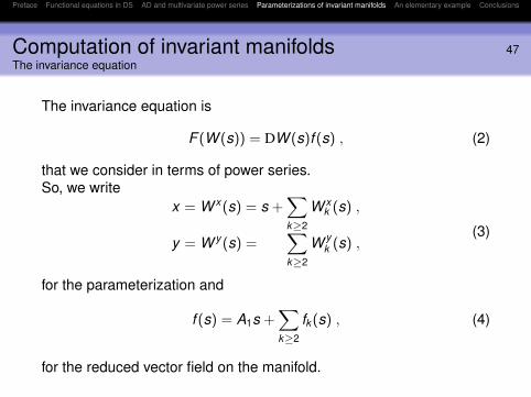
Computation of invariant manifolds 47The invariance equation
The invariance equation is
F (W (s)) = DW (s)f (s) , (2)
that we consider in terms of power series.So, we write
x = W x (s) = s +∑k≥2
W xk (s) ,
y = W y (s) =∑k≥2
W yk (s) ,
(3)
for the parameterization and
f (s) = A1s +∑k≥2
fk (s) , (4)
for the reduced vector field on the manifold.

Preface Functional equations in DS AD and multivariate power series Parameterizations of invariant manifolds An elementary example Conclusions
Computation of invariant manifolds 48Homological equations
Step k>1
From W<k (s) and f<k (s) (and [F (W<k (s))]<k , including theintermediate results), do:
1 Compute [F (W<k (s))]k .2 Solve for Wk the k -order homological equations
DWk (s)A1s − AWk (s) + DW1(s)fk (s) = Rk (s) (5)
where Wk is known from previous steps:
Wk (s) = [F (W<k (s))]k − [DW<k (s)f<k (s)]k . (6)
3 Compute [F (W≤k (s))]≤k just adding AWk (s) to [F (W<k (s))]k .

Preface Functional equations in DS AD and multivariate power series Parameterizations of invariant manifolds An elementary example Conclusions
Computation of invariant manifolds 49Solving the homological equations
We split the homological equations in two blocks:
DW xk (s)A1s − A1W x
k (s) + fk (s) = Rxk (s) + BW y
k (s) , (7)DW y
k (s)A1s − A2W yk (s) = Ry
k (s) , (8)
where Rk (s) denotes the right hand side of (5).
For the sake of simplicity, we assume A1,A2 in diagonal form:
A1 = diag(λ1, . . . , λd ),A2 = diag(λd+1, . . . , λn).
Preface Functional equations in DS AD and multivariate power series Parameterizations of invariant manifolds An elementary example Conclusions
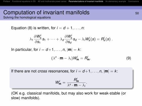
Computation of invariant manifolds 50Solving the homological equations
Equation (8) is written, for i = d + 1, . . . ,n:
λ1∂W i
k∂s1
s1 + · · ·+ λd∂W i
k∂sd
sd − λiW ik (s) = R i
k (s) .
In particular, for i = d +1, . . . ,n, |m| = k :
(λx ·m− λi )W im = R i
m. (9)
If there are not cross resonances, for i = d +1, . . . ,n, |m| = k :
W im =
R im
λx ·m− λi.
(OK e.g. classical manifolds, but may also work for weak-stable (orslow) manifolds).

Preface Functional equations in DS AD and multivariate power series Parameterizations of invariant manifolds An elementary example Conclusions
Computation of invariant manifolds 51Solving the homological equations
Equation (7) is written, for i = 1, . . . ,d :
λ1∂W i
k∂s1
s1 + · · ·+ λd∂W i
k∂sd
sd − λiW ik (s) + f i
k (s) = R ik (s) , (10)
where Rxk (s) = Rx
k (s) + BW yk (s).
Hence, for i = 1, . . . ,d , |m| = k :
(λx ·m− λi )W im + f i
m = R im. (11)

Preface Functional equations in DS AD and multivariate power series Parameterizations of invariant manifolds An elementary example Conclusions
Computation of invariant manifolds 52Solving the homological equations
For i = 1, . . . ,d , |m| = k : (λx ·m− λi )W im + f i
m = R im.
Main styles of parameterizations
Graph method. For i = 1, . . . ,d , |m| = k .
W im = 0, f i
m = R im.
Normal form method. For i = 1, . . . ,d , |m| = k :f im = 0 , W i
m =R i
m
λx ·m− λi, if λx ·m− λi 6= 0;
f im = R i
m , W im = 0, if λx ·m− λi = 0.
(d = n corresponds to normal form)

Preface Functional equations in DS AD and multivariate power series Parameterizations of invariant manifolds An elementary example Conclusions
Computation of invariant manifolds 53Cost for elementary vector fields
Complexity
Let wn,d (k) be the computational cost of solving (2) up to order k .Then,
wn,d (k) ∼ Cpd (k),
where the constant C depends on the dimension n and complexity cof the elementary vector field F , the dimension d of the manifold andthe style of parameterization.
Graph method:
wn,d (k) ∼ c pd (k) + (n − d)d pd (k). (12)
Parameterization method (with polynomial normal form):
wn,d (k) ∼ c pd (k), (13)

Preface Functional equations in DS AD and multivariate power series Parameterizations of invariant manifolds An elementary example Conclusions
An elementary example

Preface Functional equations in DS AD and multivariate power series Parameterizations of invariant manifolds An elementary example Conclusions
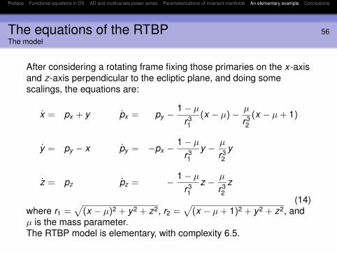
The equations of the RTBP 55Description
The RTBP models the motion of a massless body under thegravitational forces induced by two punctual bodies (primaries) incircular Keplerian motion.
Preface Functional equations in DS AD and multivariate power series Parameterizations of invariant manifolds An elementary example Conclusions
The equations of the RTBP 56The model
After considering a rotating frame fixing those primaries on the x-axisand z-axis perpendicular to the ecliptic plane, and doing somescalings, the equations are:
x = px + y px = py −1− µ
r31
(x − µ)− µ
r32
(x − µ+ 1)
y = py − x py = −px −1− µ
r31
y − µ
r32
y
z = pz pz = − 1− µr31
z − µ
r32
z
(14)where r1 =
√(x − µ)2 + y2 + z2, r2 =
√(x − µ+ 1)2 + y2 + z2, and
µ is the mass parameter.The RTBP model is elementary, with complexity 6.5.

Preface Functional equations in DS AD and multivariate power series Parameterizations of invariant manifolds An elementary example Conclusions
An elementary example 57Computation of center and center-(un)stable manifolds
RTBP has 5 equilibrium points: L1,L2,L3 are collinear, and L4,L5are triangular.Each collinear point is unstable (c × c × s), with one 4D centermanifold, 5D center-(un)stable manifolds, and 1D (un)stablemanifolds.Computation of these objects is useful in astrodynamics, and hasbeen carried out several times in the literature.The pioneers were Carles Simó’s team in 80’s, and nowadaysare used e.g. in designing space missions by ESA and NASA(see Martin Lo!).Standard technique: reduction of the dynamics to the centermanifold. This is performed through a partial normal form of theHamiltonian killing the unstable directions (6D).Here: Direct computation of the center manifold of the L1 in theEarth-Moon system.

Preface Functional equations in DS AD and multivariate power series Parameterizations of invariant manifolds An elementary example Conclusions
Benchmarks 58Run like hell
For µ ' 0.0121506 (E-M system), for L1, we have computed thecenter manifold (d = 4) with this laptop.
k product graph ratio10 4.352e−04 7.790e−03 17.9020 2.533e−02 4.048e−01 15.9830 3.582e−01 5.497e+00 15.3440 2.590e+00 3.921e+01 15.1450 1.259e+01 1.900e+02 15.0960 4.708e+01 7.104e+02 15.0870 1.460e+02 2.207e+03 15.12
The theoretical estimates for the ratio is 14.5 = 6.5 + (6− 4) · 4.
Preface Functional equations in DS AD and multivariate power series Parameterizations of invariant manifolds An elementary example Conclusions
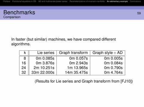
Benchmarks 59Comparison
In faster (but similar) machines, we have compared differentalgorithms.
k Lie series Graph transform Graph style + AD8 0m 0.085s 0m 0.057s 0m 0.005s
16 0m 3.876s 0m 2.943s 0m 0.084s24 2m 10.251s 1m 13.965s 0m 0.790s32 33m 22.000s 14m 35.475s 0m 4.764s
(Results for Lie series and Graph transform from [FJ10])

Preface Functional equations in DS AD and multivariate power series Parameterizations of invariant manifolds An elementary example Conclusions
Growth of the coefficients 60Fitting the growth
For k > 0, let `1(k) be the maximum of the `1 norms of the k th ordercoefficients of Wk . In log-scale ...
0.7
0.8
0.9
1
1.1
1.2
0 10 20 30 40 50 60 70k
Then:`1(k) ∼ `(k) = Aλk (log k)ck
where a = log A,b = logλ and c are estimated by
a = −1.25± 0.05 , b = −0.212± 0.008 , c = 0.252± 0.005

Preface Functional equations in DS AD and multivariate power series Parameterizations of invariant manifolds An elementary example Conclusions
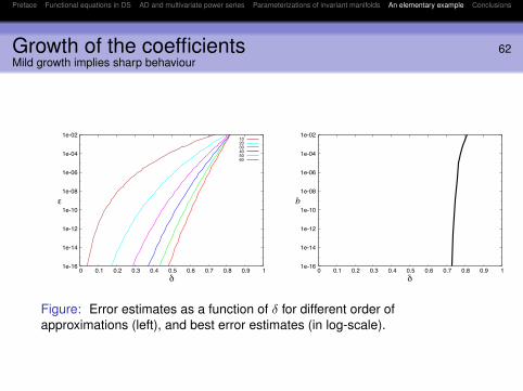
Growth of the coefficients 61Mild growth implies sharp behaviour
Assume that, for δ small enough, the expansion of W (s) for |s|∞ ≤ δis asymptotic, that is:
|W≤k (s)−W (s)|∞ ≤ `1(k + 1)δk+1 ∼ ε(δ, k) = `(k + 1)δk+1 . (15)
Following [C. Simó], the best bound b(δ) for the error in theapproximation of W (s) by W≤k (s) in the box |s|∞ ≤ δ is obtainedtaking k = k(δ) minimizing ε(δ, k). In the present case,
k(δ) =1e
exp(
(λδ)−1c
)− 1 ,
b(δ) = ε(δ, k(δ)) = A exp(−c(λδ)
1c (k(δ) + 1)
).
Hence, the mild growth of the coefficients of the expansions explainsthe behavior of the (best) error of the asymptotic approximation.
Preface Functional equations in DS AD and multivariate power series Parameterizations of invariant manifolds An elementary example Conclusions
Growth of the coefficients 62Mild growth implies sharp behaviour
1e-16
1e-14
1e-12
1e-10
1e-08
1e-06
1e-04
1e-02
0 0.1 0.2 0.3 0.4 0.5 0.6 0.7 0.8 0.9 1
102030405060
1e-16
1e-14
1e-12
1e-10
1e-08
1e-06
1e-04
1e-02
0 0.1 0.2 0.3 0.4 0.5 0.6 0.7 0.8 0.9 1
b
Figure: Error estimates as a function of δ for different order ofapproximations (left), and best error estimates (in log-scale).

Preface Functional equations in DS AD and multivariate power series Parameterizations of invariant manifolds An elementary example Conclusions
Dynamics on the center manifold 63Poincaré section
In order to analyze the dynamics on the 4D center manifold, we usethe following standard technique:
Fix an energy level H > HL1 ' −1.594171;Use Poincaré section with {z = 0}.
From different energy levels one gets a collection of 2D phaseportraits, obtaining a local-global view of the dynamics on the centermanifold.
The boundary of the intersection of the center manifold with anenergy level and the Poincaré section is a closed curve: a planarLyapunov orbit.
Other important periodic orbits are the vertical Lyapunov orbit and thehalo orbits.
Preface Functional equations in DS AD and multivariate power series Parameterizations of invariant manifolds An elementary example Conclusions
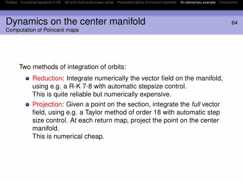
Dynamics on the center manifold 64Computation of Poincaré maps
Two methods of integration of orbits:
Reduction: Integrate numerically the vector field on the manifold,using e.g. a R-K 7-8 with automatic stepsize control.This is quite reliable but numerically expensive.Projection: Given a point on the section, integrate the full vectorfield, using e.g. a Taylor method of order 18 with automatic stepsize control. At each return map, project the point on the centermanifold.This is numerical cheap.

Preface Functional equations in DS AD and multivariate power series Parameterizations of invariant manifolds An elementary example Conclusions
Dynamics on the center manifold 65Error estimates
The error in the invariance equation:
eI(t , s0) = ||F (W (s(t)))− DW (s(t))f (s(t))||∞ ,
The error in the orbit:
eO(t , s0) = ||W (s(t))− z(t)||∞.
The error in the Hamiltonian:
eH(t , s0) = |H(W (s(t)))− H(W (s(0)))|.

Preface Functional equations in DS AD and multivariate power series Parameterizations of invariant manifolds An elementary example Conclusions
Dynamics on the center manifold 66H = −1.590
-1.2
-0.8
-0.4
0.0
0.4
0.8
1.2
-1.2 -0.8 -0.4 0.0 0.4 0.8 1.2
s2
s1
-0.15
-0.10
-0.05
0.00
0.05
0.10
0.15
-1.00 -0.95 -0.90 -0.85 -0.80
y
x

Preface Functional equations in DS AD and multivariate power series Parameterizations of invariant manifolds An elementary example Conclusions
Dynamics on the center manifoldH = −1.580
-1.2
-0.8
-0.4
0.0
0.4
0.8
1.2
-1.2 -0.8 -0.4 0.0 0.4 0.8 1.2
s2
s1
-0.15
-0.10
-0.05
0.00
0.05
0.10
0.15
-1.00 -0.95 -0.90 -0.85 -0.80
y
x

Preface Functional equations in DS AD and multivariate power series Parameterizations of invariant manifolds An elementary example Conclusions
Dynamics on the center manifold 68H = −1.570
-1.2
-0.8
-0.4
0.0
0.4
0.8
1.2
-1.2 -0.8 -0.4 0.0 0.4 0.8 1.2
s2
s1
-0.15
-0.10
-0.05
0.00
0.05
0.10
0.15
-1.00 -0.95 -0.90 -0.85 -0.80
y
x

Preface Functional equations in DS AD and multivariate power series Parameterizations of invariant manifolds An elementary example Conclusions
Dynamics on the center manifold 69H = −1.565
-1.2
-0.8
-0.4
0.0
0.4
0.8
1.2
-1.2 -0.8 -0.4 0.0 0.4 0.8 1.2
s2
s1
-0.15
-0.10
-0.05
0.00
0.05
0.10
0.15
-1.00 -0.95 -0.90 -0.85 -0.80
y
x

Preface Functional equations in DS AD and multivariate power series Parameterizations of invariant manifolds An elementary example Conclusions
The energy level H = −1.565Main periodic orbits
-0.89-0.87
-0.85-0.83
-0.81 -0.10 -0.05 0.00 0.05 0.10
-0.10-0.050.000.050.10
z
planarvertical
halohalo
xy
z

Preface Functional equations in DS AD and multivariate power series Parameterizations of invariant manifolds An elementary example Conclusions
The energy level H = −1.565 71Error estimates for the planar Lyapunov orbit
1e-16
1e-14
1e-12
1e-10
1e-08
1e-06
1e-04
1e-02
0 0.5 1 1.5 2 2.5 3
eI
t
102030405060
1e-16
1e-14
1e-12
1e-10
1e-08
1e-06
1e-04
1e-02
0 0.5 1 1.5 2 2.5 3
eH
t
102030405060
1e-16
1e-14
1e-12
1e-10
1e-08
1e-06
1e-04
1e-02
0 0.5 1 1.5 2 2.5 3
eO
t
102030405060 k T e1
PO e2PO
10 2.944806 2.48e-15 3.35e-0220 2.943184 9.99e-16 3.03e-0530 2.943083 1.67e-15 7.38e-0640 2.943068 1.44e-15 1.53e-0650 2.943065 1.67e-15 3.67e-0760 2.943065 1.44e-15 9.53e-08

Preface Functional equations in DS AD and multivariate power series Parameterizations of invariant manifolds An elementary example Conclusions
The energy level H = −1.565 72Error estimates for the vertical Lyapunov orbit
1e-16
1e-14
1e-12
1e-10
1e-08
1e-06
1e-04
1e-02
0 0.5 1 1.5 2 2.5 3
eI
t
102030405060
1e-16
1e-14
1e-12
1e-10
1e-08
1e-06
1e-04
1e-02
0 0.5 1 1.5 2 2.5 3
eH
t
102030405060
1e-16
1e-14
1e-12
1e-10
1e-08
1e-06
1e-04
1e-02
0 0.5 1 1.5 2 2.5 3
eO
t
102030405060 k T e1
PO e2PO
10 3.006224 9.99e-16 4.54e-0420 3.006243 8.88e-16 9.33e-0930 3.006243 7.77e-16 3.51e-1140 3.006243 3.89e-16 1.25e-1250 3.006243 4.37e-16 1.27e-1260 3.006243 4.37e-16 1.14e-12
Preface Functional equations in DS AD and multivariate power series Parameterizations of invariant manifolds An elementary example Conclusions
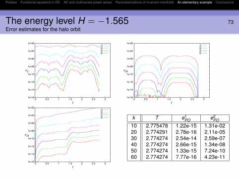
The energy level H = −1.565 73Error estimates for the halo orbit
1e-16
1e-14
1e-12
1e-10
1e-08
1e-06
1e-04
1e-02
0 0.5 1 1.5 2 2.5 3
eI
t
102030405060
1e-16
1e-14
1e-12
1e-10
1e-08
1e-06
1e-04
1e-02
0 0.5 1 1.5 2 2.5 3
eH
t
102030405060
1e-16
1e-14
1e-12
1e-10
1e-08
1e-06
1e-04
1e-02
0 0.5 1 1.5 2 2.5 3
eO
t
102030405060 k T e1
PO e2PO
10 2.775478 1.22e-15 1.31e-0220 2.774291 2.78e-16 2.11e-0530 2.774274 2.54e-14 2.59e-0740 2.774274 2.66e-15 1.34e-0850 2.774274 1.33e-15 7.24e-1060 2.774274 7.77e-16 4.23e-11

Preface Functional equations in DS AD and multivariate power series Parameterizations of invariant manifolds An elementary example Conclusions
The energy level H = −1.565A −1 : 18 period orbit around vertical orbit
-0.89-0.87
-0.85-0.83
-0.81 -0.10 -0.05 0.00 0.05 0.10
-0.10-0.050.000.050.10
z
xy
z

Preface Functional equations in DS AD and multivariate power series Parameterizations of invariant manifolds An elementary example Conclusions
The energy level H = −1.565A 1 : 9 periodic orbit around halo orbit
-0.89-0.87
-0.85-0.83
-0.81 -0.10 -0.05 0.00 0.05 0.10
-0.10-0.050.000.050.10
z
xy
z

Preface Functional equations in DS AD and multivariate power series Parameterizations of invariant manifolds An elementary example Conclusions
Further onNumerical chaos in the energy level H = −1.555
-1.2
-0.8
-0.4
0.0
0.4
0.8
1.2
-1.2 -0.8 -0.4 0.0 0.4 0.8 1.2
s2
s1
-0.15
-0.10
-0.05
0.00
0.05
0.10
0.15
-1.00 -0.95 -0.90 -0.85 -0.80
y
x

Preface Functional equations in DS AD and multivariate power series Parameterizations of invariant manifolds An elementary example Conclusions
Conclusions

Preface Functional equations in DS AD and multivariate power series Parameterizations of invariant manifolds An elementary example Conclusions
Conclusions 78
The link of the parameterization method with automaticdifferentiation provide efficient methods to compute multivariatepower series expansions of invariant manifolds.Computation of the semi-local manifold is the starting point tostudy the manifold (globalization, visualization, etc.)The methods work for conservative and dissipative systems.We can also obtain efficient methods to compute normal forms ofelementary Hamiltonians.

Preface Functional equations in DS AD and multivariate power series Parameterizations of invariant manifolds An elementary example Conclusions
Final remarks 79
AD methods are applied in many contexts:
Numerical methodsValidated methods of computation (with interval arithmetics)Sensitivity analysisDesign optimizationData assimilation and inverse problems