Comput Geosci (2014) 18:1009–1022DOI 10.1007/s10596-014-9441-z

ORIGINAL PAPER

A backward automatic differentiation frameworkfor reservoir simulation

Xiang Li · Dongxiao Zhang

Received: 29 November 2013 / Accepted: 26 August 2014 / Published online: 17 September 2014© Springer International Publishing Switzerland 2014

Abstract In numerical reservoir simulations, Newton’smethod is a concise, robust and, perhaps the most commonlyused method to solve nonlinear partial differential equa-tions (PDEs). However, as reservoir simulators incorporatemore and more physical and chemical phenomena, writingcodes that compute gradients for reservoir simulation equa-tions can become quite complicated. This paper presentsan automatic differentiation (AD) framework that is spe-cially designed for simplifying coding and simultaneouslymaintaining computational efficiency. First a parse tree fora mathematical expression is built and evaluated with thebackward mode AD, and then the derivatives with respectto the expression’s arguments are transformed to deriva-tives with respect to the PDE’s independent variables. Thefirst stage can be realized either by runtime polymorphismto gain higher flexibility or by compile-time polymorphismto gain faster execution speed; the second stage is real-ized by linear combinations of sparse vectors, which can beaccelerated by recording the target column indices. The ADframework has been implemented in an in-house reservoirsimulator. Individual tests on some complex mathemati-cal expressions were carried out to compare the speedof the manual implementation, the runtime polymorphicimplementation and the compile-time polymorphic imple-mentation of the differentiation. Then the performance ofthe three was analyzed in complete simulations. These cases

X. LiCollege of Engineering, Peking University, Room 1009,Taipingyang Building, Peking University, Beijing, Chinae-mail: lixiangcn@pku.edu.cn

D. Zhang (�)College of Engineering, Peking University, Building 60,Yannanyuan, Peking University, Beijing, Chinae-mail: dxz@pku.edu.cn

indicate that the proposed approach has good efficiency andis applicable to reservoir simulations.

Keywords Reservoir simulation · Automaticdifferentiation · Backward mode · Expression template

Mathematics Subject Classifications (2010) 65F02 ·68W02

1 Introduction

Reservoir simulation serves as a primary tool for quantita-tive reservoir management. The status of reservoirs, wells,and ground facilities are governed by nonlinear equationsand are solved after these equations are discretized in timeand in space. Explicit schemes often have numerical insta-bility in solving these types of problems, unless small timesteps are used, which lead to unacceptably slow simula-tion speeds. To ensure stability under larger time steps, acertain level of implicitness is needed. Newton’s method isthen used to solve the implicit equations; hence the resid-ual vector’s firstorder gradients with respect to the implicitunknowns are needed to assemble the Jacobian matrix.Writing analytical differentiation code by hand, known as“hand differentiation (HD)” is tedious and error prone,especially when the simulator needs to integrate manycomplicated models to model the recovery processes moreaccurately. Numerical differentiation (ND) can easily gen-erate gradients for complicated and even black-box models,but it suffers from precision and efficiency problems [32]. Infact, HD is still the most common approach in commercialsimulators, because manually optimized code produces thebest computational performance. However, it takes a largehuman effort to linearize a long and deep expression. Fur-thermore, the developer may have to keep duplicate code

1010 Comput Geosci (2014) 18:1009–1022

implementations of the same mathematical model if the sim-ulator contains different types of reservoir models, becausethe implicit unknown sets may be different. As a result, thesimulation code becomes difficult to maintain.

An alternative choice for generating gradients is auto-matic differentiation (AD), the basic principle of whichis the chain rule. Compared with ND, AD offers perfectaccuracy up to machine precision; compared with HD, ADrequires less human labor. Early research and implementa-tions of AD focused on the forward mode [4, 31] in whichthe values and derivatives are calculated simultaneously.Forward mode is more convenient for programming, but lesssuitable for producing partial derivatives for “multiple inputsingle output” functions, which are the usual cases in reser-voir simulations. A complicated physical or chemical modeloften has a long list of arguments. Let n be the dimensionof the argument vector x; “work(g)” be the computationalwork of evaluating g(x); and “work(g, ∇g)” be the com-putational work of evaluating g(x) and its derivatives withrespect to x. The work ratio of forward mode satisfies aninequality: work(g,∇g)

work(g)≥ 1 + n

c[13], where c is a positive

constant(

a special case is c = 2 when g (x) =n∏

i=1xi

),

so the additional computational work grows linearly withn. However, Wolfe [32] pointed out that if care is takenin HD code, the work ratio is usually around 1.5, andrarely exceeds 2; Baur and Strassen [3] proved that the non-scalar complexity of {g, ∇g}, with “nonscalar complexity”defined as the minimal number of nonscalar multiplicationsand divisions sufficient to compute a set of functions [8],can be reduced to lower than three times of the nonscalarcomplexity of {g}.

While the forward mode could be far from optimalwhen the argument list is long, the other category of ADalgorithms—the backward mode, also called the reversemode [23, 25], is independent of the number of arguments.The backward mode is closely related to sensitivity analy-sis [9, 10], in which the function’s derivative with respectto an intermediate variable is named as the “adjoint” of thevariable. In each elementary operation, if the adjoint of theresult and the values of the operands are known in advance,the adjoints of the operands can be calculated. So in thebackward mode, all intermediate variables are evaluatedfirst, and then the adjoints are calculated, proceeding fromthe final result to the arguments. When we give “work(g)”and work(g, ∇g)” more concrete definitions, i.e. assumethat an addition is cheaper than a multiplication and a divi-sion takes at least 50 % more work than a multiplication,and also include memory fetches/stores as the cost, it canbe proven [13] that for the backward mode, work{g,∇g}

work{g} isbounded under 5, regardless of the number of the arguments.

In general, AD tools can be divided into two classes:the source code translator and the external library. Until

today, numerous AD tools have been developed, andsome representative tools are as follows: ADIFOR—a for-ward/backward Fortran 77 code translator [6]; OpenAD—a forward/backward mode XML schema translator [26,27]; FADBAD—a forward/backward mode C++ librarybased on runtime polymorphism [5]; ADETL—a forwardmode C++ library based on expression templates [33, 34];Sacado—a forward/backward mode C++ library [21, 22],in which the forward mode is realized by expression tem-plates; and ADEPT—a backward mode C++ library basedon expression templates [15]. Source translators convertthe original code which only evaluates variables to codethat calculates corresponding gradients. This method is lessdesirable in reservoir simulators, because making changesto the program code would become less convenient. Exter-nal libraries act as extensions to the current language toprovide additional data structures and overloaded elemen-tary operators on these data types. Each data structure packsone variable value and the associated derivatives into a cap-sulation. With external libraries, the AD code will have asimilar appearance to the plain evaluating expressions, andthe change in the expression is directly reflected in the gra-dients change. External libraries are preferred in modernreservoir simulators. Researchoriented simulators, such asMRST [18] and GPRS [11], as well as commercial sim-ulators, such as Schlumberger Intersect [12], have alreadyintroduced AD libraries to simplify the coding of gradients.In a recent modification, GPRS uses ADETL to reconstructmost of its formulations and is, hence, renamed as AD-GPRS [33, 34], in which the data from basic independentvariables to the residual vectors are all AD structures. Thegradient part of the residual vector is used to construct theJacobian matrix. The heavy use of AD makes AD-GPRScompletely different from its predecessor.

The biggest obstacle to applying AD libraries to reservoirsimulators lies in computational inefficiency. The forwardmode based on operator overloading, which is the most user-friendly, may suffer from the issue of temporary objects.Upon the return of each elementary operation, the objectthat stores the result is delivered to a newly allocated tem-porary object as the returned value. The resultant object isthen destroyed upon the exiting of the current function call,and the returned object is destroyed after the function callwhich takes it as an argument. As the length of the gradi-ent vector is usually determined at runtime, the constructionand destruction of these short-life temporary objects occuron the heap memory, which causes substantial performancedeterioration of more than an order of magnitude [33]. The“expression templates” technique [1, 28] can overcome thisissue. Expression templates are a kind of compile-time poly-morphism (in comparison with runtime polymorphism).However, the work ratio of the forward mode is indepen-dent of polymorphism implementations. Sacado introduces

Comput Geosci (2014) 18:1009–1022 1011

caching and expression-level reverse mode [7] techniquesto reduce the unnecessary calculations of forward mode. Infact, Sacado tries to combine the forward mode with thebackward mode to some extent. The ADEPT has realizeda template-based backward mode with the help of globalstacks, and the benchmarks show that it has better per-formance than the runtime forward/backward AD and thetemplate based forward AD in both speed and memory use.

The backward mode is superior to the forward modewhen the expression is complicated. It naturally avoidsconstructions and copies of temporary objects and, mean-while the work ratio is independent of the argument listlength. Though the evaluation phase and the differentia-tion phase will both result in recursive function jumps,which take additional time, it is much cheaper than theheavy allocating/de-allocating operations on heap memory.In addition, with expression templates the recursive func-tions can be expanded during the compiling stage. In thiswork, we propose a backward mode AD implementationthat is independent of global variables. As this scheme isessentially thread-safe and without assessing stacks, theexpanded functions are less disruptive to CPU pipelines.

For the sake of simplicity, in the following text, werefer to the backward mode AD realized by runtime poly-morphism as the “runtime backward AD” and refer to thebackward mode AD realized by expression template as the“compile-time backward AD” The remainder of this paperis organized as follows: in Section 2, we demonstrate howto implement backward mode with runtime polymorphismor with expression templates, and provide a method to per-form variable substitution automatically and rapidly; and inSection 3, we discuss the feasibility of applying this “back-ward AD + variable substitution” procedure in a reservoirsimulator and compare the performance of the runtimebackward AD, the compile-time backward AD, and the HD.The programming language in our discussion is assumed tobe C++0x; the compiler that we use is Visual C++10.

2 Methods

2.1 The backward mode AD

2.1.1 Basic concepts of AD

The basic principle of AD is the chain rule, namely if dhdx

is known, ddx [g (h)] equals dg

dhdhdx

, where x, h, and g maybe vectors. Usually the form of g (h) is not simple andcan be decomposed into a sequence of elementary opera-tions: g (h) = gK (gK−1... (g1 (h))), where gi (i = 1 · · ·K)

stands for binary operations such as multiplications andadditions, or unary operations such as logarithms and expo-nentiations. Each elementary operation has a particular

deviation rule, e.g., (h1 × h2)′ = h′

1h2 + h′2h1, [ln (h1)]′ =

h′1

/h′

1 . The goal of AD is to create code that automatically

propagates derivatives from dhdx

to dgdx

. The intermediate

propagating process can be performed either from dg1dh

todgdh

(the forward mode), or from dgdgK

to dgdh

(the backward

mode). When propagating from dgdgK

to dgdh

, the values of allintermediate variables (gK, gK−1, · · ·g1) should be knownin advance; so, backward AD needs a standalone evaluatingphase at the beginning.

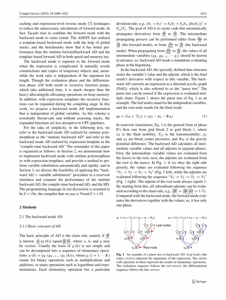
In the backward AD, the specially defined data structurestores the variable’s value and the adjoint, which is the finalresult’s derivative with respect to this variable. The back-ward AD converts an expression to a directed acyclic graph(DAG), which is also referred to as the “parse tree” Theparse tree can be reused if the expression is evaluated mul-tiple times. Figure 1 shows the parse tree of Eq. 1 as anexample. The leaf nodes stand for the independent variables,and the root node stands for the final result.

qP = (λP × T12) × (p2 − p1 − �H ) (1)

In reservoir simulations, Eq. 1 is the general form of phaseP’s flow rate from grid block 2 to grid block 1, whereλP is the fluid mobility; T12 is the transmissibility; p1

and p2 are block center pressures; and �H is the gravitypotential difference. The backward AD calculates all inter-mediate variable values and all adjoints in separate phases.First, the intermediate variable values are evaluated fromthe leaves to the root; next, the adjoints are evaluated fromthe root to the leaves. In Fig. 1, if we obey the right sidepriority, the values are evaluated following the sequence“V1 → V2 → V3 → V4” (Fig. 1 left), while the adjoints areevaluated following the sequence “V4 → V2 → V1 → V3”(Fig. 1 right). The adjoint of the root node always equals 1.By starting from this, all subordinate adjoints can be evalu-ated according to the chain rule, e.g., ∂qP

∂V2= ∂qP

∂V4

∂V4∂V2

= 1·V3.Compared with the backward mode, the forward mode eval-uates the derivatives together with the values; so, it has onlyone phase.

Fig. 1 An example of a parse tree in backward AD. Leaf nodes (theempty circles) represent the arguments of the expression. The circleswith operators in them represent the results of elementary operations.The evaluation sequence follows the red arrows; the differentiationsequence follows the blue arrows

1012 Comput Geosci (2014) 18:1009–1022

2.1.2 Backward mode by runtime polymorphism

It is natural to implement the backward AD with runtimepolymorphism, which is the case in most currently avail-able backward AD libraries. For simplicity, we call this the“runtime backward AD”. In this approach, the leaf node,the constant node and the intermediate nodes that carry ele-mentary operations are all derived from a base type. Thebase type only stores the value and the adjoint, and it willnever be involved in calculation. The derived types are dif-ferent from each other: the leaf node also stores its index;the constant node has an adjoint always being zero; and theintermediate node stores the references of its one or twooperands additionally. The building of the parse tree throughoverloaded operators is simply to pass the references ofthe two (or one) operands to its parent node correspond-ing to the operator. Then we can traverse the whole parsetree by recursively querying the children of the top par-ent node (the root node). Another difference between thederived nodes lies in their evaluating and differentiatingroutines. The base type only provides pure virtual defini-tions of these functions, while each derived type providesthe concrete realizations. For example, in the multiplicationnode—the “MulNode” class, the evaluating function is asfollows:

void MulNode::Eval (const double* Varg)

{ Right->Eval (Varg); Le�->Eval (Varg);

value = Le�->value * Right->value; }

the differentiating function is as follows:

void MulNode::Diff(double* Grad)

{ Right->adjoint = adjoint * Le�->value; Right->Diff(Grad);

Le�->adjoint = adjoint * Right->value; Le�->Diff(Grad); }

where “Varg” is an array that stores the values of the expres-sion’s arguments; “Grad” is an array that stores the outputgradients; and “Left” and “Right” are references to the leftand right operands, respectively. “Left” and “Right” are basetype pointers, which have the authority to access any derivedtypes and invoke their data and functions inherited from thebase type.

Calling the “EVal” function and the “Diff” function ofthe root node will form recursive callings of all subor-dinate “EVal” functions and all subordinate “Diff” func-tions, respectively. The recursions terminate at the leafnodes or the constant nodes. The constant node hascompletely empty evaluating function and differentiating

function; whereas, the leaf node has the evaluating functionas follows:

void Leaf::Eval(const double* Varg) { value = Varg[IDX]; }

and the differentiating function as:

void Leaf::Diff(double* Grad) { Grad[IDX] += adjoint; }

where “IDX” is the index of a leaf node. So in the leaf node,the “Eval” function is simply to get the node value from theinput array, and the “Diff” function is simply to accumulatethe gradient to the output array.

During the evaluation or the differentiation phase, thebackward mode AD need not return temporary objects. Thisis a significant advantage of the backward mode AD overthe forward mode AD. It may be argued that the construc-tion of the parse tree takes additional time. However, inreservoir simulations an expression is usually used hun-dreds of thousands of times; thus, the construction timecan be ignored. The real problem is the expensive recursivefunction jump in/out. Under certain circumstances the com-piler can automatically expand recursive functions. Unfor-tunately, however, here the compiler will reject expandingthem, because “Eval” and “Diff” are virtual functions to bedetermined dynamically and which concrete realization of“Eval” or “Diff” will be used is not known to the compiler.

2.1.3 Backward mode by expression templates

Expression templates are a kind of metaprogrammingparadigm, which attempts to utilize compilers to makeall possible choices and computations at compile timeto generate fast programs [1]. Expression templates arefirst described by Veldhuizen [28] and have led to thedevelopment of the high performance vector arithmeticlibrary Blitz++ [29]. The first expression-template-basedAD dates back to 2001 when Aubert et al. [2] applied it in aflow control problem. In recent years, expression-template-based AD has been introduced to reservoir simulators [12,33–35]. However, these AD implementations all make useof the forward mode which is convenient for application butcomputationally inefficient for sophisticated expressions.The goal of this work is to address the most complicatedexpressions in reservoir simulators with AD. Under thispremise, the backward mode may be the most appropri-ate. The recently published ADEPT [15] implemented theexpression-template-based backward mode AD, but it relieson global stacks that record indices and adjoints, making thelibrary less convenient for reservoir simulators, especiallywhen parallelization is considered.

We propose an expression-template-based backwardmode AD that is independent of global variables. For sim-plicity, we call this realization of AD the “compile-time

Comput Geosci (2014) 18:1009–1022 1013

backward AD”. The basic idea is to let the intermedi-ate nodes carry adjoints themselves and enable compiler’soptimization to the recursive calls of evaluating and differ-entiating function. With C++ templates, runtime polymor-phism can be replaced by compile-time polymorphism. Inthe compile-time backward AD, the evaluating and differ-entiating functions of the leaf node, the intermediate nodeand the constant node still keep similar forms as they are inthe runtime version. However, the type of references to theleft and right operands changes. Now they are abstract ref-erences of any type, and the type declarations themselvesbecome the template arguments of the node. For example,the compile-time version of multiplication node is definedas follows (the contents of other functions are omitted hereexcept for the construction function):

template<typename Le�Type, typename RightType>

class MulNode<Le�Type, RightType> {

public:

MulNode(Le�Type& _Le�, RightType& _Right)

{ Le� = _Le�; Right = _Right; };

void Eval(const double* Varg);

void Diff(double* Grad);

double value, adjoint;

Le�Type& Le�;

RightType& Right;

};

“MulNode” is one of the intermediate nodes. It cannot bedeclared explicitly but only be specialized upon the callingof the multiplication function, which is defined using theoperator overloading technique:

template<typename Le�Type, typename RightType>

MulNode<Le�Type, RightType> operator*(Le�Type& le�, RightType& right)

{ return MulNode<Le�Type, RightType>(le�, right); };

Both operands should be either a constant node, aleaf node, or an intermediate node. Consider an expres-sion “a*(b*c)” built by expression templates, where a, b,and c are leaf nodes. The expression will have a nestedtype expressed as “MulNode< Leaf, MulNode< Leaf,Leaf>>”. During the construction of the expression, theevaluating and differentiating function will be expandedby the compiler, because the sequence of the subordinate

function calls are completely static. The expanded “Diff”function of “a*(b*c)” is equivalent to the following:

Grad[c.IDX] = Grad[c.IDX] + a.value*b.value;

Grad[b.IDX] = Grad[b.IDX] + a.value*c.value;

Grad[a.IDX] = Grad[a.IDX] + b.value*c.value;

Mainstream C++ compilers (e.g., Visual C++, g++, IntelC++) support deep expansion to inline functions.

2.1.4 Comparison of runtime and compile-timebackward AD

In the runtime backward AD, the parse tree is built dynam-ically and stored on heap memory. All child nodes can beaccessed through the root node, i.e., the root node owns thetree. Sometimes root node A is not only used by one expres-sion, but can also be one branch under another root node B .Upon the deletion of B , destruction is executed recursivelyon its child nodes. To avoid the unexpected destruction ofA before the termination of A’s life cycle, each intermedi-ate node should count how many times it has been referredto, i.e., count how many red arrows that it launches asshown in Fig. 1. When destruction is executed to the node,the counter decreases by 1 and, when the counter equalszero, the delete-instruction is sent down to its child nodes.With this reference counting technique, it is safe to delivera dynamic parse tree to references, and then reuse it asbranches of other root nodes.

The runtime backward AD naturally allows conditionalbranches while the compile-time backward AD is less flex-ible. With all expressions being determined statically, theconditional branches are not allowed. The whole expressionshould be rewritten in different conditional branches. Addi-tionally, the templated root node always has a deep nestedtype deduced by the compiler and, thus, is hard to deliverto a reference, because the type of reference is not intu-itive. To reuse the templated root nodes as branches canbe only achieved by macro definitions. In the compile-timebackward AD, even the calling of the evaluating or differen-tiating function is not direct. We should create a templatedinterface that accepts abstract root node types:

template<typename RootType>

double RADEval(RootType& Root, const double* Varg, double* Grad)

{ Root.Eval(Varg); Root.Diff(Grad); return Root.value; };

The example code for evaluating and differentiating“a*(b*c)” with expression templates is given in Appendix 1.In addition, a more practical example is given inAppendix 2.

1014 Comput Geosci (2014) 18:1009–1022

Despite these inconveniences, as we will demonstrate inSection 3.2, the compile-time backward AD is more com-putationally efficient. So we suggest using compile-timebackward AD whenever possible and only using runtimebackward AD in conditional expressions that are not fre-quently executed, such as the well in/out flow rate. In othercases, the expression should be dissembled, with the staticparts realized by the compile-time backward AD.

2.2 The automatic variable substitution

Our ultimate goal of differentiating the complicated expres-sions is to evaluate the Jacobian matrix. With either theruntime or the compile-time backward AD, the gradients ofan expression with respect to the arguments are available. Inmost cases, however, the arguments are not the independentvariables of the reservoir simulation equations. Substitutingthe arguments with the independent variables for a functionf results in the matrix-vector multiplication, which can bewritten in general as:

fx =N∑

i = 1

(∂f

∂ai

ai,x

)(2)

where

(x1, x2, · · · , xM) is the basic variable set;(a1, a2, · · · , aN) is the argument set of f ;∂f∂ai

(i = 1, · · · , N) is already calculated by backwardmode AD;

ai,x =(

∂ai

∂x1, ∂ai

∂x2, · · · , ∂ai

∂xM

), imported from other mod-

ules;fx =

(∂f∂x1

,∂f∂x2

, · · · ,∂f

∂xM

), fx is the ultimate gradient

vector that we need to evaluate the Jacobian matrix

Variable substitutions occur frequently in reservoir simula-tions. Taking Eq. 1 as an example, under the natural variableset, which is widely accepted in compositional models, noneof the arguments λP, T12, and �H belong to the basic vari-able set. In the most popular object-oriented developmentof a reservoir simulator, useful intermediate variables, suchas transmissibilities, fluid motilities, gravity potential differ-ences and phase pressures, all with their ultimate gradientvectors, are provided by individual modules. The flow cal-culation module only takes the responsibility for evaluatingthe flow rate and assembling its derivatives.

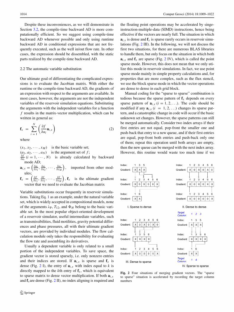
Usually a dependent variable is only related to a smallportion of the independent variables. To save space, thegradient vector is stored sparsely, i.e. only nonzero entriesand their indices are stored. If ai,x is sparse and fx isdense (Fig. 2 I), the entry of ai,x with index equal to k isdirectly mapped to the kth entry of fx , which is equivalentto sparse matrix to dense vector multiplication. If both ai,x

and fxare dense (Fig. 2 II), no index aligning is required and

the floating point operations may be accelerated by singe-instruction-multiple-data (SIMD) instructions, hence beingeffective if the vectors are nearly full. The situation in whichai,x is dense and fx is sparse rarely occurs in reservoir simu-lations (Fig. 2 III). In the following, we will not discuss thefirst two situations, for there are numerous BLAS librariesto handle them, but only focus on the situation in which bothai,x and fx are sparse (Fig. 2 IV), which is called the pointsparse mode. However, this does not mean that we only uti-lize this mode in reservoir simulations. In fact, we use pointsparse mode mainly in simple property calculations and, forproperties that are more complex, such as the flux stencil,we use the block sparse mode in which the vector operationsare dense to dense in each grid block.

Manual coding for the “sparse to sparse” combination istedious because the sparse pattern of fx depends on everysparse pattern of ai,x (i = 1, 2, . . .). The code should bemodified if any ai,x (i = 1, 2, . . .) changes its sparse pat-tern, and a catastrophic change in code will occur if the basicunknown set changes. However, the sparse patterns can stillbe merged automatically. Consider two index arrays if theirfirst entries are not equal, pop-front the smaller one andpush-back that entry to a new queue, and if their first entriesare equal, pop-front both entries and push-back only oneof them; repeat this operation until both arrays are empty,then the new queue can be merged with the next index array.However, this routine would waste too much time if we

Fig. 2 Four situations of merging gradient vectors. The “sparseto sparse” situation is accelerated by recording the target columnnumbers

Comput Geosci (2014) 18:1009–1022 1015

merge the same set of index arrays for tens of thousandsof times because, from the second time the comparing ofindexes and the allocating of arrays are unnecessary. Afterthe first time of merging, the sparse pattern of the fx isknown. We can compare ai,x with fx to determine whichcolumn of fx has the same index as the first entry of ai,x . Werecord that number, and the next time when we accumulate∂f∂ai

ai,x to fx , the first entry of ai,x is accumulated directlyto that column of fx . The same work is done for the rest ofthe entries of ai,x ; so, the next time when combining sparsevectors, each entry of ai,x knows into which column of fxit should go. This procedure is demonstrated in the lowerright part of Fig. 2. By recording target column numbers, weshift the “sparse to sparse” merging to the “sparse to dense”merging, and the latter is free of indices aligning.

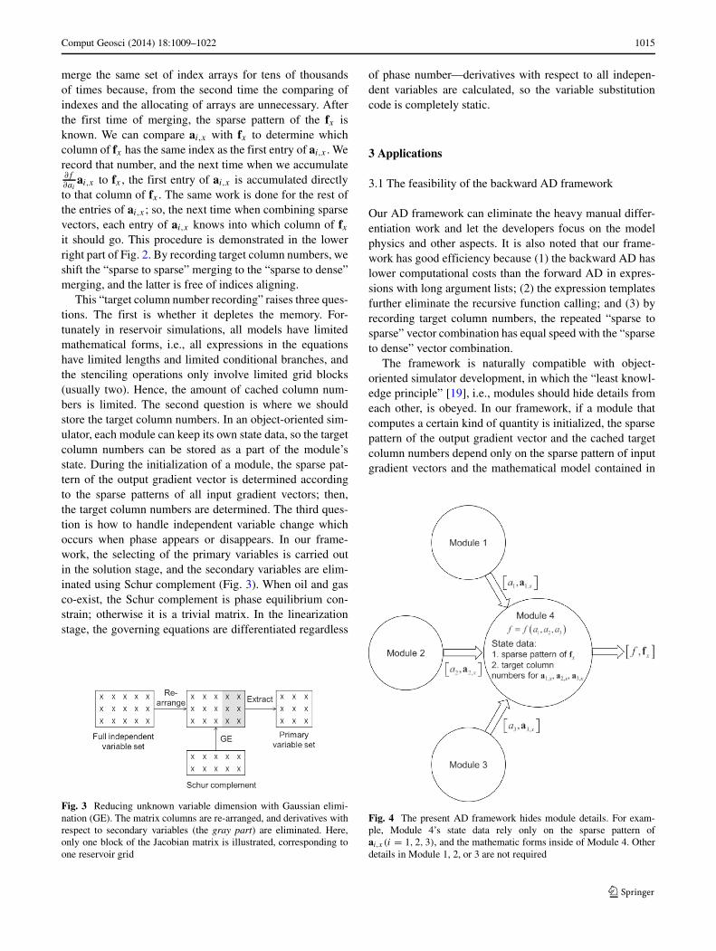
This “target column number recording” raises three ques-tions. The first is whether it depletes the memory. For-tunately in reservoir simulations, all models have limitedmathematical forms, i.e., all expressions in the equationshave limited lengths and limited conditional branches, andthe stenciling operations only involve limited grid blocks(usually two). Hence, the amount of cached column num-bers is limited. The second question is where we shouldstore the target column numbers. In an object-oriented sim-ulator, each module can keep its own state data, so the targetcolumn numbers can be stored as a part of the module’sstate. During the initialization of a module, the sparse pat-tern of the output gradient vector is determined accordingto the sparse patterns of all input gradient vectors; then,the target column numbers are determined. The third ques-tion is how to handle independent variable change whichoccurs when phase appears or disappears. In our frame-work, the selecting of the primary variables is carried outin the solution stage, and the secondary variables are elim-inated using Schur complement (Fig. 3). When oil and gasco-exist, the Schur complement is phase equilibrium con-strain; otherwise it is a trivial matrix. In the linearizationstage, the governing equations are differentiated regardless

Fig. 3 Reducing unknown variable dimension with Gaussian elimi-nation (GE). The matrix columns are re-arranged, and derivatives withrespect to secondary variables (the gray part) are eliminated. Here,only one block of the Jacobian matrix is illustrated, corresponding toone reservoir grid

of phase number—derivatives with respect to all indepen-dent variables are calculated, so the variable substitutioncode is completely static.

3 Applications

3.1 The feasibility of the backward AD framework

Our AD framework can eliminate the heavy manual differ-entiation work and let the developers focus on the modelphysics and other aspects. It is also noted that our frame-work has good efficiency because (1) the backward AD haslower computational costs than the forward AD in expres-sions with long argument lists; (2) the expression templatesfurther eliminate the recursive function calling; and (3) byrecording target column numbers, the repeated “sparse tosparse” vector combination has equal speed with the “sparseto dense” vector combination.

The framework is naturally compatible with object-oriented simulator development, in which the “least knowl-edge principle” [19], i.e., modules should hide details fromeach other, is obeyed. In our framework, if a module thatcomputes a certain kind of quantity is initialized, the sparsepattern of the output gradient vector and the cached targetcolumn numbers depend only on the sparse pattern of inputgradient vectors and the mathematical model contained in

Fig. 4 The present AD framework hides module details. For exam-ple, Module 4’s state data rely only on the sparse pattern ofai,x (i = 1, 2, 3), and the mathematic forms inside of Module 4. Otherdetails in Module 1, 2, or 3 are not required

1016 Comput Geosci (2014) 18:1009–1022

the module and do not include the details of how these inputpatterns are produced. The independence of the module iskept as much as possible (Fig. 4).

3.2 Individual tests on some expressions

Case 1 to case 6 are tests on individual expressions, forwhich we use different differentiation approaches and com-pare the performances. All cases in this paper, including thecases in Section 3.3 are compiled by Visual C++ 10 andrun on a 2.8 GHz Core 2 CPU in one core mode.

3.2.1 Validation of the compiler optimization

Case 1 yN =N∏

i=1

(i∑

j = 1xj

)

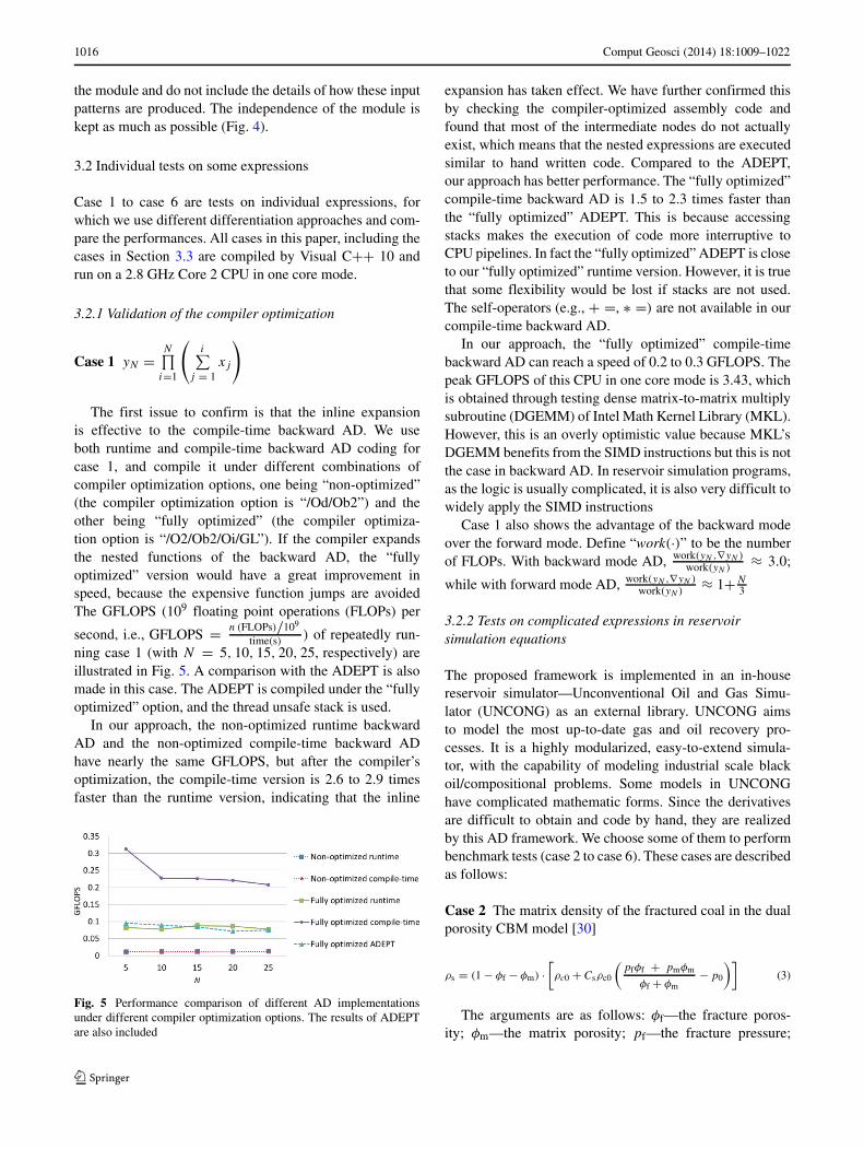
The first issue to confirm is that the inline expansionis effective to the compile-time backward AD. We useboth runtime and compile-time backward AD coding forcase 1, and compile it under different combinations ofcompiler optimization options, one being “non-optimized”(the compiler optimization option is “/Od/Ob2”) and theother being “fully optimized” (the compiler optimiza-tion option is “/O2/Ob2/Oi/GL”). If the compiler expandsthe nested functions of the backward AD, the “fullyoptimized” version would have a great improvement inspeed, because the expensive function jumps are avoidedThe GFLOPS (109 floating point operations (FLOPs) per

second, i.e., GFLOPS = n (FLOPs)/

109

time(s) ) of repeatedly run-ning case 1 (with N = 5, 10, 15, 20, 25, respectively) areillustrated in Fig. 5. A comparison with the ADEPT is alsomade in this case. The ADEPT is compiled under the “fullyoptimized” option, and the thread unsafe stack is used.

In our approach, the non-optimized runtime backwardAD and the non-optimized compile-time backward ADhave nearly the same GFLOPS, but after the compiler’soptimization, the compile-time version is 2.6 to 2.9 timesfaster than the runtime version, indicating that the inline

Fig. 5 Performance comparison of different AD implementationsunder different compiler optimization options. The results of ADEPTare also included

expansion has taken effect. We have further confirmed thisby checking the compiler-optimized assembly code andfound that most of the intermediate nodes do not actuallyexist, which means that the nested expressions are executedsimilar to hand written code. Compared to the ADEPT,our approach has better performance. The “fully optimized”compile-time backward AD is 1.5 to 2.3 times faster thanthe “fully optimized” ADEPT. This is because accessingstacks makes the execution of code more interruptive toCPU pipelines. In fact the “fully optimized” ADEPT is closeto our “fully optimized” runtime version. However, it is truethat some flexibility would be lost if stacks are not used.The self-operators (e.g., + =, ∗ =) are not available in ourcompile-time backward AD.

In our approach, the “fully optimized” compile-timebackward AD can reach a speed of 0.2 to 0.3 GFLOPS. Thepeak GFLOPS of this CPU in one core mode is 3.43, whichis obtained through testing dense matrix-to-matrix multiplysubroutine (DGEMM) of Intel Math Kernel Library (MKL).However, this is an overly optimistic value because MKL’sDGEMM benefits from the SIMD instructions but this is notthe case in backward AD. In reservoir simulation programs,as the logic is usually complicated, it is also very difficult towidely apply the SIMD instructions

Case 1 also shows the advantage of the backward modeover the forward mode. Define “work(·)” to be the numberof FLOPs. With backward mode AD, work(yN ,∇yN )

work(yN )≈ 3.0;

while with forward mode AD, work(yN ,∇yN )work(yN )

≈ 1+N3

3.2.2 Tests on complicated expressions in reservoirsimulation equations

The proposed framework is implemented in an in-housereservoir simulator—Unconventional Oil and Gas Simu-lator (UNCONG) as an external library. UNCONG aimsto model the most up-to-date gas and oil recovery pro-cesses. It is a highly modularized, easy-to-extend simula-tor, with the capability of modeling industrial scale blackoil/compositional problems. Some models in UNCONGhave complicated mathematic forms. Since the derivativesare difficult to obtain and code by hand, they are realizedby this AD framework. We choose some of them to performbenchmark tests (case 2 to case 6). These cases are describedas follows:

Case 2 The matrix density of the fractured coal in the dualporosity CBM model [30]

ρs = (1 − φf − φm) ·[ρc0 + Csρc0

(pfφf + pmφm

φf + φm− p0

)](3)

The arguments are as follows: φf—the fracture poros-ity; φm—the matrix porosity; pf—the fracture pressure;

Comput Geosci (2014) 18:1009–1022 1017

and pm—the matrix pressure. The constants are as follows:pc0—the reference coal density; Cs—the compressibility ofcoal; and p0the reference pressure. The basic variable set is{pwf, Swf, pwm, Swm}, where pwf is the fracture water pres-sure; pwm is the matrix water pressure; Swf is the fracturewater saturation; and Swm is the matrix water saturation.φf and pf are functions of (pwf, Swf); and φm and pm arefunctions of (pwm, Swm).

Case 3 The Forchheimer non-Darcy flow [16] for gasThe volumetric flow rate qgsatisfies the following:

∇�g = 1

C1

(μg

KkrgA

)qg + C2

C1βρg

(qg

A

)2(4)

qg is then expressed as the positive root of this quadraticequation. The arguments of qg’s expression are as follows:∇�g—potential gradient of gas phase; μg—gas viscosity;krg—relative permeability of gas; and ρg—gas density. Theconstants are C1, C2, K , A and β. The independent variableset is

{po, Sw, Sg, Rs

}(black oil model). The dependences

between the arguments and the basic variable set also fol-low the black oil model. The constants are merged beforecalculation.

Case 4 Tubing flow friction force in the multi-segment well(MSWell) model [17]

pf = ρ

(2Cff Vm |Vm|

D

)L (5)

where

ρ is the average fluid density, weighted by phase vol-ume fractions;

Cf is a unit converting factor;f is the Fanning friction factor;

Vm is the average velocity;D is well diameter;L is well segment length.

The Fanning friction factor—f is calculated using Haa-land’s correlation [14]:

f −0.5 = −3.6 lg

[6.9

Re+( ε

3.7D

)1.11]

(6)

whereε is the roughness factor of the tube wall;Re is the Reynolds number: Re = Cr

ρVmDμ

, where Cr isa unit converting factor; and μ is the average fluid viscosity,weighted by phase volume fractions.

The arguments are: ρ, μ, and Vm; the constantsare Cf , D, L, εCr. The independent variable set is{p, Vm, αg, αw, Rs

}(black oil MSWell model). The depen-

dence between the arguments and the basic variable set

also follows the black oil MSWell model. The constants aremerged before calculation.

Case 5 Gas drift velocity for liquid + gas flow in theMSWell model [24]

Vgd = A · B · (Ku)i · (Vc)i−1 ·√(ρl)i−1√(ρg)i· B +√

(ρl)i−1 · A

(7)

whereSubscript “i−1” denotes variable in the “downstream”

well segment, the segment to which the fluid in segment i

flows;

A = (1 − αgC0

)i−1 , where αg is gas holdup and C0 is a

profile parameter;B = (

αgC0)i

Ku is the critical Kutateladze number;Vc is the characteristic velocity;ρg is the gas density;ρl is the average liquid density: ρl =

(αoρo + αwρw)/(αo + αwρw) (αo + αw) ; where αw is

water holdup; αo is oil holdup (αo = 1 − αw − αg), andρo, ρw are oil and water density, respectively.

In the black oil MSWell model, the independentvariable set is

{p, Vm, αg, αw, Rs

}. ρo is a function

of (p, Rs); ρg and ρw are both functions of p; Ku andVc are both functions of

(p, αg, αw, Rs

); and C0 is a

function of(p, Vm, αg, αw, Rs

). Assuming that ρo, ρg,

ρw αg Ku Vc and C0, as well as their gradient vec-tor with respect to the basic variable set, have already beenprovided by other modules.

Case 6 Peaceman’s formula [20] to calculate well index(WI)

WIx = hx√

kykz

/⎡⎢⎣ln

⎛⎜⎝0.28

rw

√kyD2

z + kzD2y√

ky + √kz

⎞⎟⎠+ s

⎤⎥⎦

WIy = hy√

kzkx

/[ln

(0.28

rw

√kxD2

z + kzD2x√

kx + √kz

)+ s

](8)

WIz = hz√

kxky

/⎡⎢⎣ln

⎛⎜⎝0.28

rw

√kyD2

x + kxD2y√

kx +√ky

⎞⎟⎠+ s

⎤⎥⎦

WI =(

WI2x + WI2

y + WI2z

)1/2

where kx, ky and kz are arguments; Dx, Dy, Dz, hx, hy,

hz, rw and s are constants; and kx, ky and kz are variablepermeabilities related to the reservoir independent variableset—

{po, Sw, Sg, Rs

}. The constants are merged before

calculation.

1018 Comput Geosci (2014) 18:1009–1022

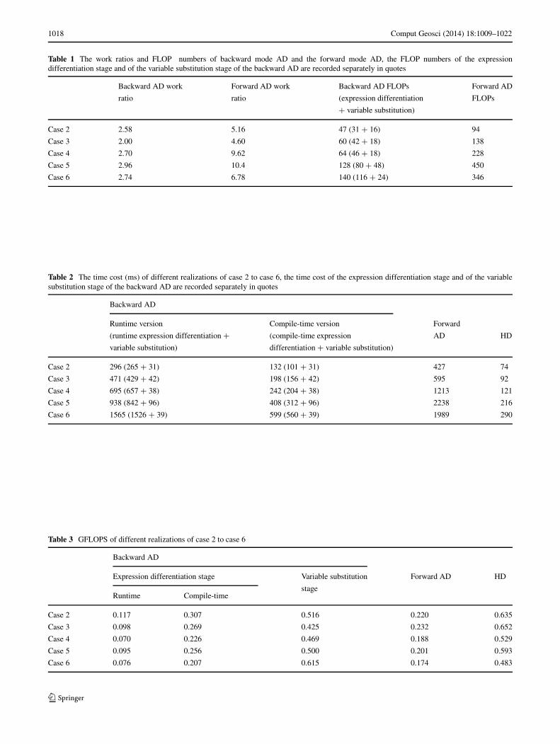
Table 1 The work ratios and FLOP numbers of backward mode AD and the forward mode AD, the FLOP numbers of the expressiondifferentiation stage and of the variable substitution stage of the backward AD are recorded separately in quotes

Backward AD work Forward AD work Backward AD FLOPs Forward AD

ratio ratio (expression differentiation FLOPs

+ variable substitution)

Case 2 2.58 5.16 47 (31 + 16) 94

Case 3 2.00 4.60 60 (42 + 18) 138

Case 4 2.70 9.62 64 (46 + 18) 228

Case 5 2.96 10.4 128 (80 + 48) 450

Case 6 2.74 6.78 140 (116 + 24) 346

Table 2 The time cost (ms) of different realizations of case 2 to case 6, the time cost of the expression differentiation stage and of the variablesubstitution stage of the backward AD are recorded separately in quotes

Backward AD

Runtime version Compile-time version Forward

(runtime expression differentiation + (compile-time expression AD HD

variable substitution) differentiation + variable substitution)

Case 2 296 (265 + 31) 132 (101 + 31) 427 74

Case 3 471 (429 + 42) 198 (156 + 42) 595 92

Case 4 695 (657 + 38) 242 (204 + 38) 1213 121

Case 5 938 (842 + 96) 408 (312 + 96) 2238 216

Case 6 1565 (1526 + 39) 599 (560 + 39) 1989 290

Table 3 GFLOPS of different realizations of case 2 to case 6

Backward AD

Expression differentiation stage Variable substitution Forward AD HD

Runtime Compile-timestage

Case 2 0.117 0.307 0.516 0.220 0.635

Case 3 0.098 0.269 0.425 0.232 0.652

Case 4 0.070 0.226 0.469 0.188 0.529

Case 5 0.095 0.256 0.500 0.201 0.593

Case 6 0.076 0.207 0.615 0.174 0.483

Comput Geosci (2014) 18:1009–1022 1019

Table 4 Description ofreservoir simulation problems Model type Grid size Well block number

Case 7 Gas water 25,000 50

Case 8 Gas water 260,985 159

Case 9 Black oil 43,644 270

Case 10 Black oil 368,326 10

Case 11 Compositional (9 components) 324 2

Case 12 Compositional (9 components) 8748 6

For each case, we use the runtime backward AD, thecompile-time backward AD the forward AD, and the HD,respectively, to evaluate the expression and its derivativeswith respect to the arguments. In the backward AD andthe HD versions, the gradients are transformed from beingwith respect to the arguments to being with respect to thebasic variables after the expressions are differentiated withthe target column recording technique. The HD code com-pletely mimics the derivation process of backward modeAD; thus, its FLOP number equals that of the backwardAD, which may not be optimal but serves as a reference. Inforward AD versions, if the input argument is a dependentvariable, we store its derivatives with respect to the basicvariables as a dense vector before the calculation begins,and the derivatives with respect to the basic variables arecalculated automatically when variables are merged, so thevariable transformation stage is not needed. The forwardAD is basically implemented by FADBAD++ v2.1 usingthe heap-based mode to allow the gradient vectors being ofvariable lengths; however we modified part of the sourcecode to minimize the expensive allocating/de-allocating oftemporary objects on heap memory when an operator func-tion is returned, using the “right-value reference” technique,which is supported by C++0x. The work ratios (definedas in Section 3.2.1) and the FLOP numbers of the back-ward AD and of the forward AD are recorded in Table 1.All FLOP numbers are counted rigorously, with no dis-tinctions between elementary operations and transcendentaloperations being made. Each case of each version is com-piled under the “fully optimized” compiler option and run106 times. The time costs of the four approaches foreach case are recorded in Table 2; the GFLOPS of theseapproaches for each case are recorded in Table 3. Case 2 tocase 6 are already sorted by the FLOP number. From theresults, we can conclude the following:

1. The backward mode AD has a much lower work ratiothan the forward mode AD.

2. The compile-time backward AD is 3.0 to 5.0 times thespeed of the forward AD, and 2.2 to 2.9 times the speedof the runtime backward AD but only about 0.5 timesthe speed of HD.

3. The variable substitution takes a considerable frac-tion of time, and if the length of the independent

variable set grows, the time cost by variable substitutionwill increase, hence lessening the overall performancedeterioration caused by automatic differentiation ofexpressions.

4. In the backward AD, the GFLOPS (of either the expres-sion differentiation stage or the variable substitutionstage) is not affected much by the number of arithmeticoperators or the number of arguments. Transcenden-tal operators would affect GFLOPS (case 4 and case6) because evaluating a transcendental function takesmore CPU clock cycles. This situation is also true in theforward AD and the HD.

3.3 Tests in complete simulation processes

The final question is how much the proposed AD frameworkslows down the simulator. We answer this by comparingthe time cost of the linearization work realized by differentmethods in complete reservoir simulations.

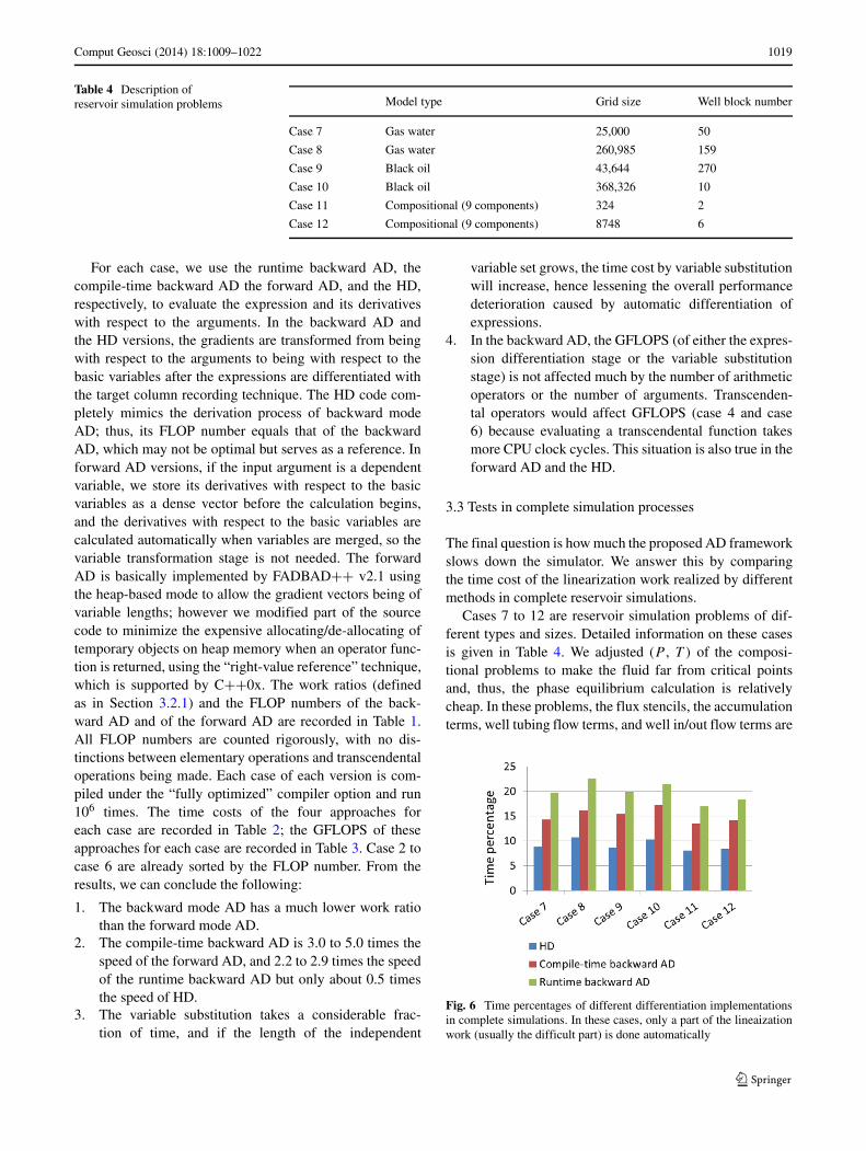
Cases 7 to 12 are reservoir simulation problems of dif-ferent types and sizes. Detailed information on these casesis given in Table 4. We adjusted (P , T ) of the composi-tional problems to make the fluid far from critical pointsand, thus, the phase equilibrium calculation is relativelycheap. In these problems, the flux stencils, the accumulationterms, well tubing flow terms, and well in/out flow terms are

Fig. 6 Time percentages of different differentiation implementationsin complete simulations. In these cases, only a part of the lineaizationwork (usually the difficult part) is done automatically

1020 Comput Geosci (2014) 18:1009–1022

linearized by the runtime backward AD or the compile-timebackward AD, and the variables are substituted automat-ically. Lower level modules, such as mobilities, potentialdifferences, permeabilities and porosities are programmedwith the HD because they are quite simple. So, only a part ofthe linearization work is done automatically. For each casewith each differentiation method, the time spent on this partof the work is recorded during the simulation (with a timerbeing accurate to microseconds), and its percentage to thetotal time is calculated, which is plotted in Fig. 6. Percent-ages of the HD implementation are also included, to serveas references.

We can see that this part of the linearization work onlyaccounts for a small portion of the total time, for most ofthe time is consumed by the linear solver, table lookingand phase equilibrium calculation (compositional model).The performance deterioration mainly comes from the back-ward AD phase; meanwhile, the variable substitution phasemay take a considerable amount of time. As the time ratiobetween the backward AD and the HD has been improvedto a small value (in single digits), the additional time costincurred by the AD is not obvious for the whole simulation,even with the runtime version.

4 Conclusions

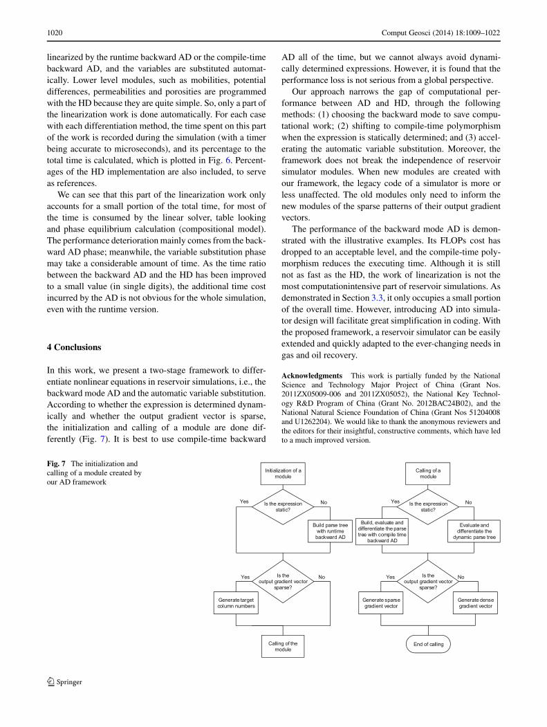
In this work, we present a two-stage framework to differ-entiate nonlinear equations in reservoir simulations, i.e., thebackward mode AD and the automatic variable substitution.According to whether the expression is determined dynam-ically and whether the output gradient vector is sparse,the initialization and calling of a module are done dif-ferently (Fig. 7). It is best to use compile-time backward

AD all of the time, but we cannot always avoid dynami-cally determined expressions. However, it is found that theperformance loss is not serious from a global perspective.

Our approach narrows the gap of computational per-formance between AD and HD, through the followingmethods: (1) choosing the backward mode to save compu-tational work; (2) shifting to compile-time polymorphismwhen the expression is statically determined; and (3) accel-erating the automatic variable substitution. Moreover, theframework does not break the independence of reservoirsimulator modules. When new modules are created withour framework, the legacy code of a simulator is more orless unaffected. The old modules only need to inform thenew modules of the sparse patterns of their output gradientvectors.

The performance of the backward mode AD is demon-strated with the illustrative examples. Its FLOPs cost hasdropped to an acceptable level, and the compile-time poly-morphism reduces the executing time. Although it is stillnot as fast as the HD, the work of linearization is not themost computationintensive part of reservoir simulations. Asdemonstrated in Section 3.3, it only occupies a small portionof the overall time. However, introducing AD into simula-tor design will facilitate great simplification in coding. Withthe proposed framework, a reservoir simulator can be easilyextended and quickly adapted to the ever-changing needs ingas and oil recovery.

Acknowledgments This work is partially funded by the NationalScience and Technology Major Project of China (Grant Nos.2011ZX05009-006 and 2011ZX05052), the National Key Technol-ogy R&D Program of China (Grant No. 2012BAC24B02), and theNational Natural Science Foundation of China (Grant Nos 51204008and U1262204). We would like to thank the anonymous reviewers andthe editors for their insightful, constructive comments, which have ledto a much improved version.

Fig. 7 The initialization andcalling of a module created byour AD framework

Comput Geosci (2014) 18:1009–1022 1021

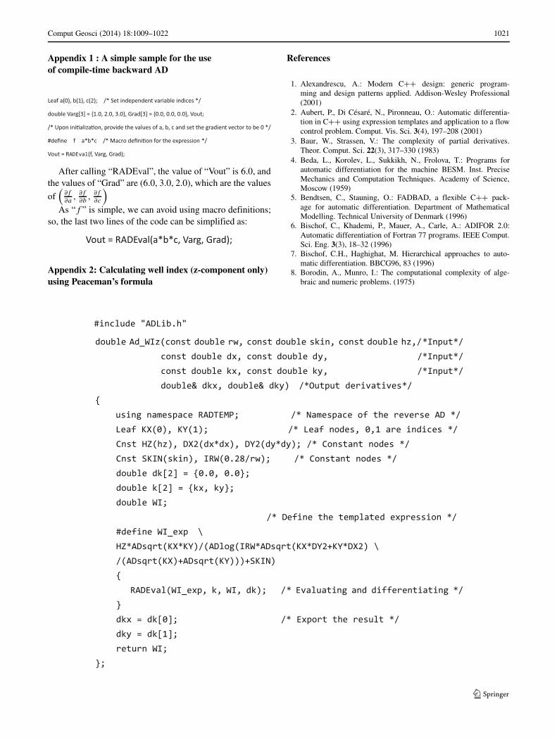
Appendix 1 : A simple sample for the useof compile-time backward AD

Leaf a(0), b(1), c(2); /* Set independent variable indices */

double Varg[3] = {1.0, 2.0, 3.0}, Grad[3] = {0.0, 0.0, 0.0}, Vout;

/* Upon ini�aliza�on, provide the values of a, b, c and set the gradient vector to be 0 */

#define f a*b*c /* Macro defini�on for the expression */

Vout = RADEval(f, Varg, Grad);

After calling “RADEval”, the value of “Vout” is 6.0, andthe values of “Grad” are (6.0, 3.0, 2.0), which are the values

of(

∂f∂a

,∂f∂b

,∂f∂c

)

As “f ” is simple, we can avoid using macro definitions;so, the last two lines of the code can be simplified as:

Vout = RADEval(a*b*c, Varg, Grad);

Appendix 2: Calculating well index (z-component only)using Peaceman’s formula

References

1. Alexandrescu, A.: Modern C++ design: generic program-ming and design patterns applied. Addison-Wesley Professional(2001)

2. Aubert, P., Di Cesare, N., Pironneau, O.: Automatic differentia-tion in C++ using expression templates and application to a flowcontrol problem. Comput. Vis. Sci. 3(4), 197–208 (2001)

3. Baur, W., Strassen, V.: The complexity of partial derivatives.Theor. Comput. Sci. 22(3), 317–330 (1983)

4. Beda, L., Korolev, L., Sukkikh, N., Frolova, T.: Programs forautomatic differentiation for the machine BESM. Inst. PreciseMechanics and Computation Techniques. Academy of Science,Moscow (1959)

5. Bendtsen, C., Stauning, O.: FADBAD, a flexible C++ pack-age for automatic differentiation. Department of MathematicalModelling. Technical University of Denmark (1996)

6. Bischof, C., Khademi, P., Mauer, A., Carle, A.: ADIFOR 2.0:Automatic differentiation of Fortran 77 programs. IEEE Comput.Sci. Eng. 3(3), 18–32 (1996)

7. Bischof, C.H., Haghighat, M. Hierarchical approaches to auto-matic differentiation. BBCG96, 83 (1996)

8. Borodin, A., Munro, I.: The computational complexity of alge-braic and numeric problems. (1975)

1022 Comput Geosci (2014) 18:1009–1022

9. Cacuci, D.G.: Sensitivity theory for nonlinear systems. I. Non-linear functional analysis approach. J. Math. Phys. 22(12), 2794–2802 (1981)

10. Cacuci, D.G.: Sensitivity theory for nonlinear systems. II. Exten-sions to additional classes of responses. J. Math. Phys. 22(12),2803–2812 (1981)

11. Cao, H.: Development of techniques for general purpose simula-tors. Stanford University (2002)

12. DeBaun, D., Byer, T., Childs, P., Chen, J., Saaf, F., Wells, M., Liu,J., Cao, H., Pianelo, L., Tilakraj, V.: An extensible architecturefor next generation scalable parallel reservoir simulation. In: SPEReservoir Simulation Symposium (2005)

13. Griewank, A.: On automatic differentiation. Mathematical Pro-gramming: recent developments and applications 6, 83–107(1989)

14. Haaland, S.E.: Simple and explicit formulas for the friction fac-tor in turbulent pipe flow. J. Fluids Eng.; (United States) 105(1)(1983)

15. Hogan, R.J.: Fast reverse-mode automatic differentiation usingexpression templates in C+. Submitted to ACM Trans. Math.Softw. (2014)

16. Huang, H., Ayoub, J.: Applicability of the Forchheimer equa-tion for non-Darcy flow in porous media. SPE J. 13(1), 112–122(2008)

17. Jiang, Y.: Techniques for modeling complex reservoirs andadvanced wells. Stanford University (2007)

18. Lie, K.A., Krogstad, S., Ligaarden, I.S., Natvig, J.R., Nilsen,H.M., Skaflestad, B.: Open-source MATLAB implementationof consistent discretisations on complex grids. Comput. Geosci.16(2), 297–322 (2012)

19. Lieberherr, K.J., Holland, I.M.: Assuring good style for object-oriented programs. IEEE Softw. 6(5), 38–48 (1989)

20. Peaceman, D.W.: Interpretation of well-block pressures in numer-ical reservoir simulation. Soc. Pet. Eng. J. 18(03), 183–194(1978)

21. Phipps, E., Pawlowski, R.: Efficient expression templates foroperator overloading-based automatic differentiation. In: RecentAdvances in Algorithmic Differentiation, pp. 309-319. Springer(2012)

22. Phipps, E.T., Bartlett, R.A., Gay, D.M., Hoekstra, R.J.: Large-scale transient sensitivity analysis of a radiation-damaged bipolarjunction transistor via automatic differentiation. In: Advances inautomatic differentiation, pp. 351-362. Springer (2008)

23. Rall, L.B.: Automatic differentiation: techniques and applications(1981)

24. Shi, H., Holmes, J., Durlofsky, L., Aziz, K., Diaz, L., Alkaya, B.,Oddie, G.: Drift-flux modeling of two-phase flow in wellbores.SPE J. 10(1), 24–33 (2005)

25. Speelpenning, B.: Compiling fast partial derivatives of functionsgiven by algorithms. In. Illinois Univ., Urbana (USA). Dept. ofComputer Science (1980)

26. Utke, J.: OpenAD: Algorithm implementation user guide. Techni-cal Mem (2004)

27. Utke, J., Naumann, U., Fagan, M., Tallent, N., Strout, M.,Heimbach, P., Hill, C., Wunsch, C.: OpenAD/F: A modular open-source tool for automatic differentiation of Fortran codes. ACMTrans. Math. Softw. (TOMS) 34(4), 18 (2008)

28. Veldhuizen, T.: Expression templates. C++ Report 7(5), 26–31(1995)

29. Veldhuizen, T.: Arrays in blitz++. In: Computing in object-oriented parallel environments, pp. 223-230. Springer (1998)

30. Wei, Z., Zhang, D.: Coupled fluid-flow and geomechanics fortriple-porosity/dual-permeability modeling of coalbed methanerecovery . International Journal of Rock Mechanics and MiningSciences 47(8), 1242–1253 (2010)

31. Wengert, R.: A simple automatic derivative evaluation program.Commun. ACM 7(8), 463–464 (1964)

32. Wolfe, P.: Checking the calculation of gradients. ACM Trans.Math. Softw. (TOMS) 8(4), 337–343 (1982)

33. Younis, R., Aziz, K.: Parallel automatically differentiable data-types for next-generation simulator development. In: SPE Reser-voir Simulation Symposium (2007)

34. Younis, R.M.: Modern advances in software and solution algo-rithms for reservoir simulation. Stanford University (2011)

35. Zhou, Y., Tchelepi, H., Mallison, B.: Automatic differentiationframework for compositional simulation on unstructured gridswith multi-point discretization schemes. In: SPE Reservoir Simu-lation Symposium (2011)