automatic design of turbomachinery blading using gpu...
TRANSCRIPT
Universidad Politécnica de Madrid
Escuela Técnica Superior de Ingenieros Aeronáuticos
Automatic Design of TurbomachineryBlading Using GPU Accelerated
Adjoint Compressible Flow Analysis
Tesis Doctoral
Ricardo Puente Rico
Ingeniero Aeronáutico
Madrid, 2017

Departamento de Motopropulsión y Termofluidodinámica
Escuela Técnica Superior de Ingenieros Aeronáuticos
Automatic Design of Turbomachinery
Blading Using GPU Accelerated
Adjoint Compressible Flow Analysis
AutorRicardo Puente RicoIngeniero Aeronáutico
DirectorRoque Corral GarcíaDoctor Ingeniero Aeronáutico
Madrid, Septiembre 2017


Tribunal nombrado por el Sr. Rector Magfco. de la Universidad Politécnica de Madrid,
el día ...... de .......................... de 2017.
Presidente: D. Benigno Lázaro
Vocal: D. Shahrokh Shahpar
Vocal: D. Tom Verstraete
Vocal: Dª. Ana Carpio
Secretario: D. Jose Manuel Vega
Suplente: D. Jorge Ponsín
Suplente: Dª. Raquel Gómez
Realizado el acto de defensa y lectura de la Tesis el día ......... de ........................... de
2017 en la E.T.S.I Aeronáuticos.
Calificación .......................................
El presidente Los vocales
El secretario


Abstract
This work presents the development of an Automatic Design Optimization tool, with
the declared objective that it be actually practical in the context of aerodynamic
design of turbomachinery components. For that, the requirements are: that it solves a
realistic design problem fulfilling stringent quality criteria, that the results can be readily
integrated in daily workflow, that the turnaround times are faster than conventional
human driven designs, and that is robust enough that is does not need human intervention
once the procedure is initiated.
The starting point has been the existence of a set of validated design tools used routinely
in the usual human driven process, comprising geometry generation, flow analysis, and
solution postprocessing tools, developed at the Tecnology & Methods department at
Industria de TurboPropulsores S.A. Initial conceptual studies and development of an
adjoint flow solver (integral part of a sensitivity calculation methodology) were performed
by Fernando Gisbert in his doctoral thesis [1].
During the course of this thesis, these design tools have been interfaced in a seamless
manner to build a fully automatic chain for airfoil geometry definition and evaluation
in terms of thermodynamic efficiency and manufacturability. The result is that the
output of this chain can be used by an external optimization algorithm to propose a
high performance geometry, without more human input than that of the specification
of the design problem. Regarding this issue, routine industrial design often involves an
number of informal or implicit criteria. An effort has been done to bring these to light so
that they can be translated to algorithmic language.
Critical stages of the geometry generation and analysis have been accelerated by the use
of general purpose GPU computing, achieving very low turnaround times. For that, the
7

relevant computer science knowledge has been developed and is presented.
Results of different design exercises carried out at different stages of development
are provided, illustrating the improvements in speed and capabilities of the growing
environment. At its current state, turbomachinery components with a quality comparable
to that of a human design with strict requirements can be generated in a fraction of the
time.
Resumen
Este trabajo presenta el desarrollo de una herramienta de Diseńo y Optimización
Automático con el objetivo declarado de que sea realmente práctica en el contexto del
diseńo aerodinámico de componentes de turbomaquinaria. Para ello, los requerimientos
son: que resuelva un problema realista, cumpliendo estrictos criterios de calidad, que
el resultado se pueda integrar inmediatamente en el flujo de trabajo estándar, que los
tiempos por iteración de diseńo sean menores que los del diseńo convencional dirigido
por personas, y que sea lo suficientemente robusto como para que no haya necesidad de
intervención humana una vez se lanza el proceso.
El punto de partida es un conjunto de herramientas de diseńo validadas y usadas
rutinariamente en el proceso dirigido por personas, que comprenden herramientas de
generación de geometría, análisis fluido y postproceso de las soluciones, desarrolladas en el
departamento de Tecnología y Métodos de Industria de TurboPropulsores S.A. Estudios
conceptuales y el desarrollo de un resolvedor de las ecuaciones de Navier-Stokes adjuntas
(parte integral de un método de cálculo de sensitividades) fueron llevados a cabo por
Fernando Gisbert en su tesis doctoral [1].
A lo largo del curso de esta tesis, dichas herramientas de diseńo se han comunicado de una
forma fluida para construir una cadena totalmente automática de definición de geometrías
de álabes de turbomaquinaria, y su evaluación en términos de eficiencia termodinámica
y manufacturabilidad. El resultado es que la salida de esta cadena puede ser empleado
por un algoritmo externo de optimización para proponer geometrías de altas prestaciones,
sin más intervención humana que la especificación del problema de diseńo. Atendiendo a
este aspecto, el diseńo rutinario frecuentemente requiere de ciertos criterios que no están
expresados formalmente, o son implícitos. Se ha realizado un esfuerzo para sacarlos a la
9

luz de modo que puedan ser traducidos a un lenguaje algorítmico.
Etapas cruciales de la generación de geometría y del análisis han sido aceleradas mediante
el uso genérico de las capacidades de computación de la GPUs, consiguiendo unos
tiempos por iteración muy bajos. Para ello, el necesario conocimiento de la ciencia de
la computación ha sido desarrollado y se expone aquí.
Los resultados de diferentes ejercicios de diseńo efectuados en distintas etapas del
desarrollo del sistema se presentan, ilustrando las mejoras en velocidad y capacidad del
entorno de diseńo automático. Es su estado actual, álabes de turbomaquinaria con una
calidad comparable a la de un diseńo humano se pueden generar en una fracción del
tiempo.

Acknowledgements
En primer lugar, quisiera agradecer a Roque Corral, el director de esta tesis, por aceptar
mi propusta de trabajo. Aún en cuanto he tenido libertad para desarrollar mi actividad
en el sentido en el que he creído conveniente, en las ocasiones en las que he tenido la
tentación de tomar atajos, me ha disuadido de ello.
En segundo, agradezco también al resto de compańeros del departamento de Tecnología
de Simulación de ITP. Sin el trabajo que ellos realizan ha diario, yo no hubiera podido
sacar el mío adelante.
Por último, gracias a los miembros del tribunal por aceptar a valorar este trabajo.
11

A man provided with paper, pencil and rubber, and subject to strict discipline, is in effect
a universal machine.
Alan Turing
Contents
1 Fundamentals of turbomachinery airfoil design 29
1.1 Generic methodology . . . . . . . . . . . . . . . . . . . . . . . . . . . . . . 30
1.1.1 Conceptual design phase . . . . . . . . . . . . . . . . . . . . . . . . 30
1.1.2 Preliminary and detailed design phases . . . . . . . . . . . . . . . . 35
1.1.2.1 Throughflow design and analysis . . . . . . . . . . . . . . 36
1.1.2.2 Blade to blade design and analysis . . . . . . . . . . . . . 38
1.1.2.3 Three dimensional stacking . . . . . . . . . . . . . . . . . 38
1.1.2.4 High fidelity analysis and feedback generation . . . . . . . 39
1.2 Aerodynamics of turbomachinery components . . . . . . . . . . . . . . . . 42
1.2.1 Blade to blade aerodynamics. Generalities . . . . . . . . . . . . . . 43
1.2.2 Secondary flows. Generalities . . . . . . . . . . . . . . . . . . . . . 46
1.2.3 Three dimensional design techniques . . . . . . . . . . . . . . . . . 50
1.2.4 Unsteady effects. Generalities . . . . . . . . . . . . . . . . . . . . . 50
1.2.5 Low Pressure Turbine airfoils . . . . . . . . . . . . . . . . . . . . . 54
1.2.6 High Pressure Turbine airfoils. . . . . . . . . . . . . . . . . . . . . . 59
1.3 Multistage matching . . . . . . . . . . . . . . . . . . . . . . . . . . . . . . 60
2 Optimization methods 63
2.1 Derivative free methods . . . . . . . . . . . . . . . . . . . . . . . . . . . . 64
13

2.1.1 Population based methods . . . . . . . . . . . . . . . . . . . . . . . 65
2.1.1.1 Surrogate modeling techniques . . . . . . . . . . . . . . . 67
2.1.2 Direct search methods . . . . . . . . . . . . . . . . . . . . . . . . . 71
2.2 Local derivative based methods . . . . . . . . . . . . . . . . . . . . . . . . 73
2.3 Constraint treatment . . . . . . . . . . . . . . . . . . . . . . . . . . . . . . 74
2.3.1 Lagrange multipliers . . . . . . . . . . . . . . . . . . . . . . . . . . 75
2.3.2 Penalty functions . . . . . . . . . . . . . . . . . . . . . . . . . . . . 76
2.3.2.1 Augmented Lagrangian . . . . . . . . . . . . . . . . . . . 77
2.3.2.2 Interior point methods . . . . . . . . . . . . . . . . . . . . 77
2.3.2.3 Kreisselmeier-Steinhauser method. . . . . . . . . . . . . . 78
2.4 Selecting a single solution . . . . . . . . . . . . . . . . . . . . . . . . . . . 79
2.4.1 Normalization . . . . . . . . . . . . . . . . . . . . . . . . . . . . . . 79
2.4.2 Preference articulation methods . . . . . . . . . . . . . . . . . . . . 80
2.5 Sensitivity computation techniques . . . . . . . . . . . . . . . . . . . . . . 83
2.5.1 Finite differences . . . . . . . . . . . . . . . . . . . . . . . . . . . . 83
2.5.2 Complex step differentiation . . . . . . . . . . . . . . . . . . . . . . 83
2.5.3 Algorithmic differentiation . . . . . . . . . . . . . . . . . . . . . . . 83
2.5.4 Adjoint method . . . . . . . . . . . . . . . . . . . . . . . . . . . . . 84
2.5.4.1 One-shot optimization . . . . . . . . . . . . . . . . . . . . 86
3 Automatic design environment 87
3.1 Overview of the design methodology . . . . . . . . . . . . . . . . . . . . . 92
3.2 Automatic design loop . . . . . . . . . . . . . . . . . . . . . . . . . . . . . 97
3.2.1 Overview . . . . . . . . . . . . . . . . . . . . . . . . . . . . . . . . 97
3.2.2 Objective functions and gradient computation. . . . . . . . . . . . . 98
3.2.3 3D unstructured RANS base solver. . . . . . . . . . . . . . . . . . . 100
3.2.4 Adjoint solver. . . . . . . . . . . . . . . . . . . . . . . . . . . . . . . 103
3.2.5 Scalarization approach and constraint treatment. . . . . . . . . . . 107
3.2.6 Optimization algorithms. . . . . . . . . . . . . . . . . . . . . . . . . 109
3.3 Generalized adjoint analysis. . . . . . . . . . . . . . . . . . . . . . . . . . . 109
4 Implementation in Graphics Processor Units 113
4.1 GPU accelerated non-linear and discrete adjoint Navier-Stokes solvers . . . 114
4.1.1 Code performance . . . . . . . . . . . . . . . . . . . . . . . . . . . . 126
4.2 GPU accelerated mesh deformation . . . . . . . . . . . . . . . . . . . . . . 127
4.3 Validation. . . . . . . . . . . . . . . . . . . . . . . . . . . . . . . . . . . . . 130
5 Applications 133
5.1 Realistic 3D blading for low pressure turbines . . . . . . . . . . . . . . . . 133
5.1.1 Introduction . . . . . . . . . . . . . . . . . . . . . . . . . . . . . . . 133
5.1.2 Geometry definition . . . . . . . . . . . . . . . . . . . . . . . . . . . 134
5.1.3 Objective and constraint functions . . . . . . . . . . . . . . . . . . 135
5.1.3.1 Flow dependent functionals . . . . . . . . . . . . . . . . . 135
5.1.3.2 Geometrical constraints . . . . . . . . . . . . . . . . . . . 136
5.1.3.3 Solver settings. . . . . . . . . . . . . . . . . . . . . . . . . 136
5.1.4 Results . . . . . . . . . . . . . . . . . . . . . . . . . . . . . . . . . . 137
5.1.4.1 High aspect ratio, hade angle non-orthogonal vane . . . . 137
5.1.4.2 Low aspect ratio, hade angle, non-orthogonal vane . . . . 143
5.1.5 Conclusions . . . . . . . . . . . . . . . . . . . . . . . . . . . . . . . 146
5.2 Outlet Guide Vane stacking line modifications to minimize losses in an
S-Shaped duct . . . . . . . . . . . . . . . . . . . . . . . . . . . . . . . . . . 146
5.2.1 Problem description and set up . . . . . . . . . . . . . . . . . . . . 148
5.2.1.1 Base geometry and design space . . . . . . . . . . . . . . . 148
5.2.2 Optimization: objectives and constraints . . . . . . . . . . . . . . . 150
5.2.3 Numerical set up . . . . . . . . . . . . . . . . . . . . . . . . . . . . 152
5.2.4 Results . . . . . . . . . . . . . . . . . . . . . . . . . . . . . . . . . . 152
5.2.5 Conclusions . . . . . . . . . . . . . . . . . . . . . . . . . . . . . . . 160
5.3 Trade off study between efficiency and rotor forced response . . . . . . . . 160
5.3.1 Optimization methodology . . . . . . . . . . . . . . . . . . . . . . . 162
5.3.2 Rotor forcing model . . . . . . . . . . . . . . . . . . . . . . . . . . 166
5.3.3 Results . . . . . . . . . . . . . . . . . . . . . . . . . . . . . . . . . . 168
5.3.3.1 Flow analysis at 10%, 50% and 90% span . . . . . . . . . 169
5.3.3.2 Outlet flow field and forcing analysis . . . . . . . . . . . . 173
5.3.3.3 Loss decomposition and circumferentially averaged analysis 174
5.3.3.4 Stacking line effect . . . . . . . . . . . . . . . . . . . . . . 176
5.3.4 Conclusions . . . . . . . . . . . . . . . . . . . . . . . . . . . . . . . 177
6 Conclusions 179
6.1 Concluding remarks . . . . . . . . . . . . . . . . . . . . . . . . . . . . . . . 179
6.2 Future work . . . . . . . . . . . . . . . . . . . . . . . . . . . . . . . . . . . 181
Bibliography 183
A Analytical derivation of cost function flow sensitivities. 201
B Adjoint Boundary Conditions. 209
List of Figures
1.0.1 Aircraft engine cutaway illustration. Source: Internet . . . . . . 29
1.1.1 Velocity triangles for a turbine stage. . . . . . . . . . . . . . . . 31
1.1.2 Original Smith chart. Source: [2] . . . . . . . . . . . . . . . . . . . . 34
1.1.3 Smith’s enthalpy-kinetic energy ratio. Source: [2] . . . . . . . . . 34
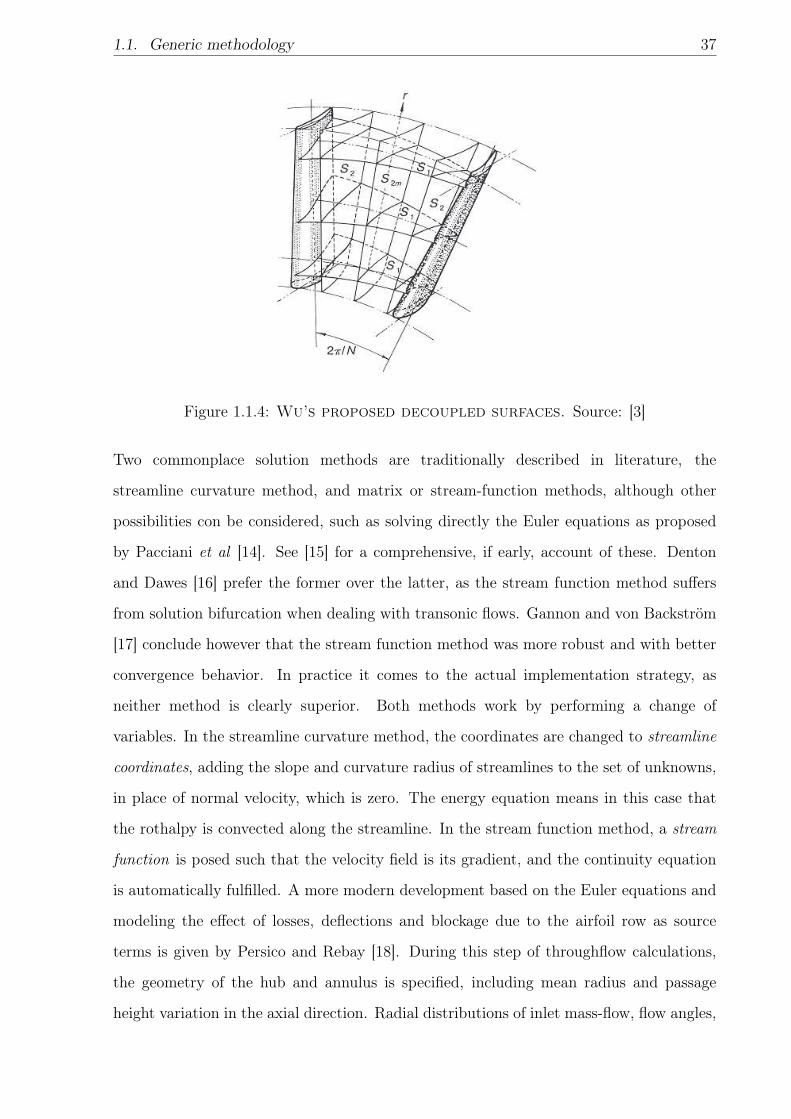
1.1.4 Wu’s proposed decoupled surfaces. Source: [3] . . . . . . . . . . . . 37
1.2.1 Definition of displacement thickness. . . . . . . . . . . . . . . . . 43
1.2.2 Shape factor in developing boundary layers. Laminar in blue,
transitional in red. . . . . . . . . . . . . . . . . . . . . . . . . . . . . 43
1.2.3 Friction factor as a function of Reynolds number. Source: [4] . 44
1.2.4 Vorticity patterns at the outlet of an airfoil cascade. . . . . 47
1.2.5 Horseshoe vortex around a cylinder. . . . . . . . . . . . . . . . . 47
1.2.6 Secondary flow development seen from the leading edge. . . . 48
1.2.7 Wakes across blade rows. . . . . . . . . . . . . . . . . . . . . . . . . 51
1.2.8 Wake induced transition diagram. Source: [5] . . . . . . . . . . . . 52
1.2.9 Wake jet effect. Source:[6] . . . . . . . . . . . . . . . . . . . . . . . . 52
1.2.10Sketch of loss variation with fr. . . . . . . . . . . . . . . . . . . . . 53
1.2.11Ultra high lift loading shape. . . . . . . . . . . . . . . . . . . . . . 56
1.2.12Front and aft loaded shape types. . . . . . . . . . . . . . . . . . . 56
1.2.13LPT profile types. Left, thick. Right, Thin. . . . . . . . . . . . . 57
17
1.2.14Separation bubble. Source: wikipedia . . . . . . . . . . . . . . . . . . 58
1.2.15Schlieren visualization of a transonic turbine cascade.
Overview and shock-bl interaction detail. Source: Web-page
of Institute of Propulsion Technology, DLR. . . . . . . . . . . . . . . . . . 59
1.2.16Sketch of shock-boundary layer interactions. . . . . . . . . . . 60
1.3.1 Multirow workflow. . . . . . . . . . . . . . . . . . . . . . . . . . . . . 62
2.0.1 Pareto frontier. Source: Johann Dréo, Wikipedia. . . . . . . . . . . . 64
2.1.1 ANN network layout. Source: Wikipedia. . . . . . . . . . . . . . . . . 69
2.1.2 1D Kriging interpolation. . . . . . . . . . . . . . . . . . . . . . . . . 69
2.1.3 Left, Simplex method candidate point generation. Right,
Shrinking when candidates are not accepted. . . . . . . . . . . . 72
2.3.1 Penalty functions. Left, interior penalty. Right, exterior
penalty. . . . . . . . . . . . . . . . . . . . . . . . . . . . . . . . . . . . . 76
2.4.1 Performance of the weighted sum method. . . . . . . . . . . . . . 81
3.1.1 standard aerodynamic design loop. . . . . . . . . . . . . . . . . . . 92
3.1.2 XBlade interface. . . . . . . . . . . . . . . . . . . . . . . . . . . . . . 93
3.1.3 Block semi-unstructured mesh. . . . . . . . . . . . . . . . . . . . . 95
3.2.1 Automatic aerodynamic design loop. . . . . . . . . . . . . . . . . . 96
3.2.2 Mesh deformation in a blade to blade plane. . . . . . . . . . . . 98
3.2.3 Hybrid-cell grid and associated dual mesh. . . . . . . . . . . . . . 101
4.1.1 Reverse Cuthill-McKee ordering to minimize cache-misses. . . 117
4.1.2 Mesh split in 16 sub-domains using the ParMETIS library
routines. . . . . . . . . . . . . . . . . . . . . . . . . . . . . . . . . . . . . 120
4.1.3 Reverse Cuthill-McKee followed by an ordering by groups
to avoid simultaneous memory access within a group. . . . . . . 121
4.1.4 Adjoint Navier Stokes solver performance. . . . . . . . . . . . . 126
4.2.1 Barycentric coordinates in a triangle. . . . . . . . . . . . . . . . 129
4.3.1 Adjoint and Finite differences sensitivity computation. . . . . 131
4.3.2 design sections with representative spanwise locations. . . . . 131
5.1.1 GA of a typical low pressure turbine . . . . . . . . . . . . . . . . 133
5.1.2 Left, airfoil parametrization. Right, design sections with
representative spanwise locations. . . . . . . . . . . . . . . . . . . 134
5.1.3 Optimization convergence. High aspect ratio case. . . . . . . . 138
5.1.4 Blade-to-blade loading (top) and blading (bottom). High
aspect ratio case. . . . . . . . . . . . . . . . . . . . . . . . . . . . . . . 138
5.1.5 Outlet plane analysis. High aspect ratio case. . . . . . . . . . . 139
5.1.6 Helicity contours. Left, human design. Right, automatic
design. High aspect ratio case. . . . . . . . . . . . . . . . . . . . . . 140
5.1.7 Streaklines at hub, with negative axial velocity spots. Left,
human design. Right, automatic design. High aspect ratio case.141
5.1.8 Streak lines at tip ,with negative axial velocity spots. Left,
human design. Right, automatic design. High aspect ratio case.141
5.1.9 Airfoil streaklines and control sections, with negative axial
velocity spots. . . . . . . . . . . . . . . . . . . . . . . . . . . . . . . . 142
5.1.10Left, optimization history. Right, thickness constraint
fulfillment. Low aspect ratio case. . . . . . . . . . . . . . . . . . 142
5.1.11Blade-to-blade loading (top) and blading (bottom). Low
aspect ratio case. . . . . . . . . . . . . . . . . . . . . . . . . . . . . . . 143
5.1.12Outlet plane analysis. Low aspect ratio case. . . . . . . . . . . 144
5.1.13Airfoil streaklines and control sections, with negative axial
velocity spots. . . . . . . . . . . . . . . . . . . . . . . . . . . . . . . . 145
5.1.14Streaklines at hub, with negative axial velocity spots. Left,
human design. Right, automatic design. High aspect ratio case.145
5.1.15Streak lines at tip, with negative axial velocity spots. Left,
human design. Right, automatic design. High aspect ratio case.145
5.2.1 Duct location within the engine architecture. . . . . . . . . . . 149
5.2.2 Left, stacking line definition. Right, mesh view . . . . . . . . . . 150
5.2.3 Flow angle (left) and KSI (right) at the exit plane. . . . . . . 151
5.2.4 Contours of circumferentially averaged static pressure in
kpa (left), and axial momentum in m/s (right). . . . . . . . . . . . 152
5.2.5 Optimization results. . . . . . . . . . . . . . . . . . . . . . . . . . . . 153
5.2.6 Circumferentially averaged distributions of KSI (left),
mass-flow per station arc-length (center), and flow angle
(right). . . . . . . . . . . . . . . . . . . . . . . . . . . . . . . . . . . . . . 154
5.2.7 Circumferentially averaged pressure in kpa (top), axial
pressure gradient in kpa/m (middle), and pressure adjoint in
kpa−1 (bottom) evaluated at hub. . . . . . . . . . . . . . . . . . . . . 155
5.2.8 Contours of circumferentially averaged pressure field: p (kpa).156
5.2.9 Contours of circumferentially averaged adjoint pressure
field: p (kpa−1). . . . . . . . . . . . . . . . . . . . . . . . . . . . . . . . . 156
5.2.10Contours of circumferentially averaged axial momentum
field: ρu (m/s). . . . . . . . . . . . . . . . . . . . . . . . . . . . . . . . . 157
5.2.11Contours of circumferentially averaged adjoint axial mo-
mentum field: ρu (s/m). . . . . . . . . . . . . . . . . . . . . . . . . . . 157
5.2.12Separated flow visualization: Wall streamlines and region
of negative axial velocity: vx (m/s). . . . . . . . . . . . . . . . . . 159
5.2.13Critical point classification. . . . . . . . . . . . . . . . . . . . . . . 159
5.2.14Wall streamlines against velocity divergence contours: ∇ ·
v ((ms)−1). . . . . . . . . . . . . . . . . . . . . . . . . . . . . . . . . . . . 159
5.3.1 Blade parametrization. . . . . . . . . . . . . . . . . . . . . . . . . . . 164
5.3.2 Rotor crossing a non-homogeneous pressure field. . . . . . . . . 167
5.3.3 Campbell diagram of the considered rotor. X is the radial
direction, from hub to tip. Y is the tangential direction,
in the rotor from PS to SS. Z is the rotating axis, from LE
towards TE. . . . . . . . . . . . . . . . . . . . . . . . . . . . . . . . . . 167
5.3.4 Pareto front. . . . . . . . . . . . . . . . . . . . . . . . . . . . . . . . . 168
5.3.5 τ and S fields at hub. Top, Opt U. Bottom, Opt L. . . . . . . . . 170
5.3.6 τ and S fields at midspan. Top, Opt U. Bottom, Opt L.. . . . . . 170
5.3.7 τ and S fields at tip. Top, Opt U. Bottom, Opt L. . . . . . . . . 171
5.3.8Mis distributions. . . . . . . . . . . . . . . . . . . . . . . . . . . . . . . 172
5.3.9 Pressure, shock function, and loss coefficient fields at the
outlet plane. Left, Opt L geometry. Right, Opt U geometry. 173
5.3.10Forcing functions. Above, model function. Below, computed
unsteady forcing. . . . . . . . . . . . . . . . . . . . . . . . . . . . . . . 174
5.3.11Isosurfaces of Mis = 1 and Mis = 1.4 . . . . . . . . . . . . . . . . . . . 175
5.3.12Circumferentially averaged radial distributions. . . . . . . . . 176


List of Tables
4.1 Computational time share breakdown. CPU (Intel Xeon 3.6GHz), GPU
(NVIDIA Quadro 4000). Test case 1: ∼ 7 · 105 grid nodes,∼ 80 DOF. . . . 113
4.2 Comparison of representative properties of a modern CPU and a modern
GPU. . . . . . . . . . . . . . . . . . . . . . . . . . . . . . . . . . . . . . . . 115
4.3 Speed up achieved in mesh deformation according to hardware and
algorithmic improvements. Baseline, CPU loop over edges. Mesh size:
∼ 1.5 · 106 nodes. . . . . . . . . . . . . . . . . . . . . . . . . . . . . . . . . 129
4.4 Computational time share breakdown. CPU (Intel Xeon 3.6GHz), GPU
(NVIDIA GeFORCE 780). Test case 2: ∼ 1.5 · 106 grid nodes,∼ 80 DOF. . 130
5.1 Operating conditions. . . . . . . . . . . . . . . . . . . . . . . . . . . . . . . 150
5.2 Optimization results. . . . . . . . . . . . . . . . . . . . . . . . . . . . . . . 153
5.3 Boundary conditions . . . . . . . . . . . . . . . . . . . . . . . . . . . . . . 165
5.4 Loss decomposition . . . . . . . . . . . . . . . . . . . . . . . . . . . . . . 176
5.5 Computationally predicted performance. . . . . . . . . . . . . . . . . . . . 176
23


Nomenclature
Roman Symbols
A Aspect ratio
cf Friction coefficient
Cpp−pLE
pLE−pTE, pressure coefficient
fr Reduced frequency
H Boundary layer shape factor
h Helicity
KSI Kinetic energy losses
M Mach number
R(u) Residual of the RANS equations
Re Reynolds number
u Conservative flow variables
u∗√τw/ρ, friction velocity
v Adjoint flow variables
y+ ρu∗yµ
, non dimensional wall distance
Zw Zweiffel coefficient
Abbreviations
25
ADO Automatic Design Optimization
CFD Computational Fluid Dynamics
CPU Central Processing Unit
GPU Graphics Processing Unit
GUI Graphical User Interface
HPT High Pressure Turbine
LE Leading edge of an airfoil
LPC Low Pressure Compressor
LPT Low Pressure Turbine
LRS Left Running Shock
NLCO Non Linear Constrained optimization algorithm
NURBS Non Rational Uniform B-Splines
PDE Partial Differential Equation
PS Pressure side of an airfoil
RRS Right Running Shock
SS Suction side of an airfoil
TE Trailing edge of an airfoil
Greek Symbols
ω Vorticity
α Flow angle
δ∗ Boundary layer displacement thickness
η Thermodynamic efficiency

27
µ Dynamic viscosity
Φ Massflow coefficient
π Pressure ratio
Ψ Loading coefficient
θ∗ Boundary layer momentum thickness
ϕ Design parameters
Superscripts
T Transposed
Mathematical Symbols
G 3 Third order (curvature) continutity class curve
H Heaviside funciton

Chapter 1
Fundamentals of turbomachinery airfoil
design
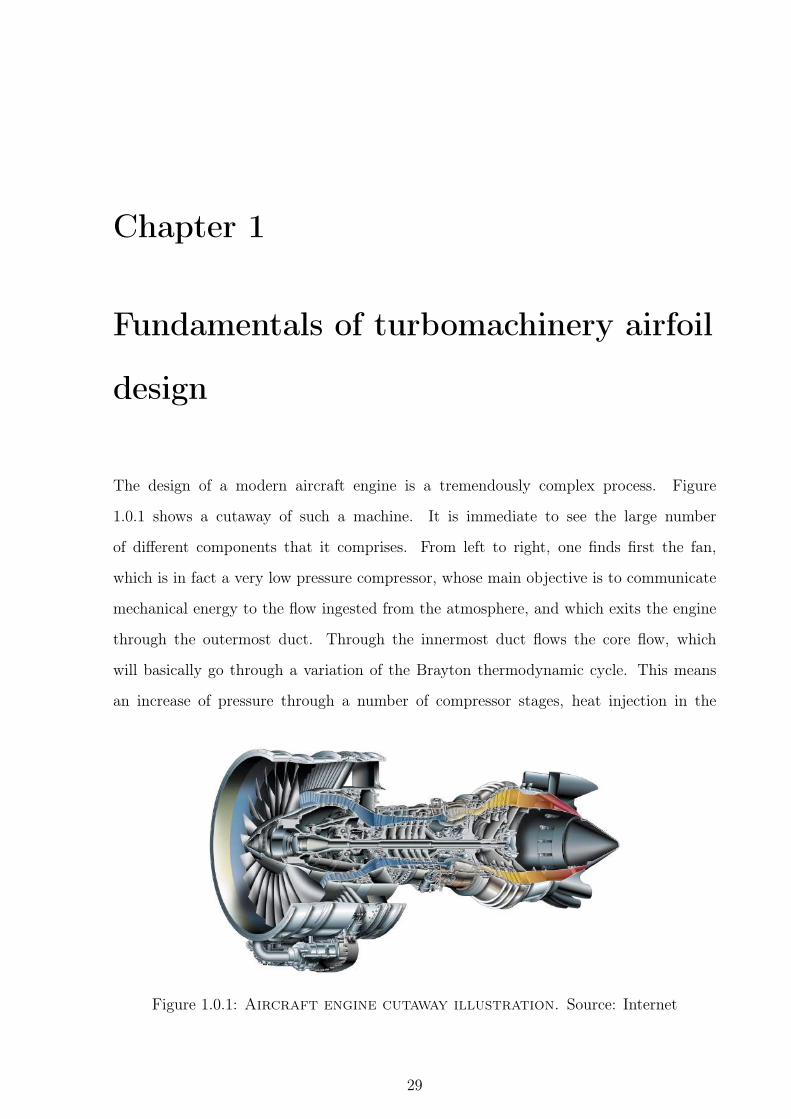
The design of a modern aircraft engine is a tremendously complex process. Figure
1.0.1 shows a cutaway of such a machine. It is immediate to see the large number
of different components that it comprises. From left to right, one finds first the fan,
which is in fact a very low pressure compressor, whose main objective is to communicate
mechanical energy to the flow ingested from the atmosphere, and which exits the engine
through the outermost duct. Through the innermost duct flows the core flow, which
will basically go through a variation of the Brayton thermodynamic cycle. This means
an increase of pressure through a number of compressor stages, heat injection in the
Figure 1.0.1: Aircraft engine cutaway illustration. Source: Internet
29
30 Chapter 1. Fundamentals of turbomachinery airfoil design
combustion chamber, and expansion across the several turbine stages. Just regarding
aerothermodynamics the working airflow, ignoring issues such as structural design, moving
parts and auxiliary systems, the problem of aeroengine design is complex enough. In order
to arrive to a final product, a number of decisions need to have been made, for example,
what the thermodynamic cycle variables need to be, i.e. pressure ratios and heat input
to provide with a given machine power requirement. Then, structural constraints and
efficiency considerations dictate that the total work done needs to be split in a number
of stages. Each component will operate in a different flow regime in terms of pressure,
temperature and flow speed. As such, the design of a given component follows a specific
set of rules and needs of specialized knowledge. A division of labor is then mandatory, an
efficient and reliable aeroengine cannot be designed by a single team or person.
In this chapter, the process of turbomachinery airfoil design will described, in order to
introduce the topic of this thesis, which is the automatic design of Low Pressure Turbines.
1.1 Generic methodology
1.1.1 Conceptual design phase
The design of a turbomachinery component starts with the definition of its mission.
This means the specification of the power consumption or output, depending on whether
speaking about a compressor or a turbine. Once this is fixed, the thermodynamic working
cycle has to be determined. Without delving to deep into the subject, the first principle of
thermodynamics relates the work done on an open adiabatic system proportionally with
both mass-flow and total temperature jump. This gives two main design variables for the
specification of the thermodynamic cycle. Restrictions are placed on mass-flow due to
size constraints, and on temperature due to material limits. It is normally the case that
a given pressure ratio is unattainable due to constraints in a single step, thus a certain
number of sub-steps or stages will need to be defined, with their associated work split.
In the so called one dimensional design of each stage, in addition to the stage loading,
the mean characteristics of the airfoils of each stage will be defined. These are the
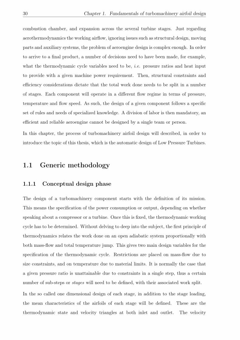
thermodynamic state and velocity triangles at both inlet and outlet. The velocity
1.1. Generic methodology 31
Figure 1.1.1: Velocity triangles for a turbine stage.
triangles are nothing more than the flow velocity vectors in the plane of projection of
a 2D airfoil shape (see figure 1.1.1 for a turbine example, in a compressor the tangential
velocity u goes in the opposite sense). This one dimensional design phase is carried out
with simple analytical tools coupled with performance correlations. The latter provide
with an estimation of efficiency so that the thermodynamic state computation can be
more accurate. These correlations necessarily cannot include much physics, due to the
simple geometrical data and overall quantities that they must be fed. Some examples
historically used include the Ainley-Mathieson [7], the Craig-Cox [8], and the Kacker-
Okapuu [9] correlations. In practice, these are currently used outside of academia, since
they rely in experiments performed in outdated rigs. Industrial operators use proprietary
correlations developed under their own research programs. In this phase, the performance
and characteristics of the components are quantified with a number of non dimensional
parameters. These are useful to have immediate understanding of the flow regime and
to be able to relate to existing rigs. In order to extract the relevant parameters the
Vaschy-Buckingham π theorem is used, which tells us that if there are k variables and n
fundamental units, there will be k − n non dimensional groups that close the problem.
But how those parameters are constructed is an open problem. Depending on the actual
data available or the application (design, turbine-compressor matching, comparison of
experimental data between rigs, scaling of an existing machine preserving operation point,
etc...), an analyst will choose which parameters are more useful. But broadly speaking,
some common ones are enumerated below:
1. Aspect ratio (A = h/cax): Overall relationship between height and axial chord. It
32 Chapter 1. Fundamentals of turbomachinery airfoil design
is important when assessing the extent of the influence of end-wall boundary layers
in the main flow, or if even a main-flow can be considered. It is also relevant when
considering structural issues.
• Pitch to chord ratio (p/Cax): Relative measure of the width of the passage between
adjacent airfoils. Directly related to the total number of airfoils, it will determine the
overall airfoil loading level. Aerodynamically speaking, an optimum value will exist,
but structural, weight and cost considerations may decide against it. In literature
also the inverse ratio, the solidity σ, has been historically used.
• Reynolds number (Re = ρUCax/µ): Ratio between the order of magnitude of
convective and viscous terms in the Navier-Stokes flow equations. It will inform
on the potential behavior of the boundary layer, laminar or turbulent, and advising
on the presence of potential transition spots.
• Mach number (M = U/a): Ratio between the actual flow speed and sound speed.
Indicates the effects of compressibility, including whether to expect shock waves or
not.
• Corrected mass-flow (m√RgT0
AP0): Written in this form, the influence of machine size
and thermodynamic state is absorbed, and the operation point between different
machines can be compared.
• Corrected rotational speed ( Ωr√γRgT0
): In rotating machines, the peripheral speed
can be non dimensionalised with a representative sound speed. Also useful when
comparing operation points.
• Degree of reaction (R = ∆hs|rotor∆hs|stage ): Ratio between static enthalpy increment in the
rotor and that of the total stage. With the next two parameters, it characterizes
the velocity triangles of a combined rotor-stator stage.
• Mass-flow coefficient (Φ = VaxΩr
): Axial velocity relative to tangential rotor velocity.
Increasing it decreases the global stage turning, as the mass-flow contributing to
total power is increased, or for a given mass-flow it will reduce the available area.
1.1. Generic methodology 33
• Loading coefficient (Ψ = ∆H0
(Ωr)2): Enthalpy delta relative to rotor energy input. For
a given total machine power, the higher this coefficient, the less stages. For a stage,
it implies higher global turning (considering a fixed mass-flow coefficient). To which
extent the turning is divided between rows is determined in conjunction with the
degree of reaction.
• Efficiency parameters: There are countless ways to quantify thermodynamic losses
within turbomachinery, but in the end, they have to be characterized by a non
dimensional number.
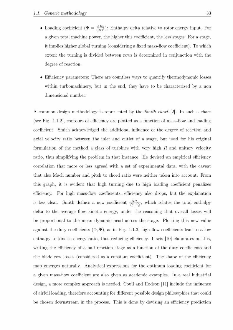
A common design methodology is represented by the Smith chart [2]. In such a chart
(see Fig. 1.1.2), contours of efficiency are plotted as a function of mass-flow and loading
coefficient. Smith acknowledged the additional influence of the degree of reaction and
axial velocity ratio between the inlet and outlet of a stage, but used for his original
formulation of the method a class of turbines with very high R and unitary velocity
ratio, thus simplifying the problem in that instance. He devised an empirical efficiency
correlation that more or less agreed with a set of experimental data, with the caveat
that also Mach number and pitch to chord ratio were neither taken into account. From
this graph, it is evident that high turning due to high loading coefficient penalizes
efficiency. For high mass-flow coefficients, efficiency also drops, but the explanation
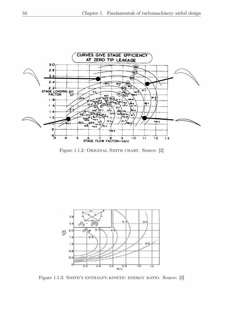
is less clear. Smith defines a new coefficient ∆H0
V 21 +V 2
2, which relates the total enthalpy
delta to the average flow kinetic energy, under the reasoning that overall losses will
be proportional to the mean dynamic head across the stage. Plotting this new value
against the duty coefficients (Φ,Ψ), as in Fig. 1.1.3, high flow coefficients lead to a low
enthalpy to kinetic energy ratio, thus reducing efficiency. Lewis [10] elaborates on this,
writing the efficiency of a half reaction stage as a function of the duty coefficients and
the blade row losses (considered as a constant coefficient). The shape of the efficiency
map emerges naturally. Analytical expressions for the optimum loading coefficient for
a given mass-flow coefficient are also given as academic examples. In a real industrial
design, a more complex approach is needed. Coull and Hodson [11] include the influence
of airfoil loading, therefore accounting for different possible design philosophies that could
be chosen downstream in the process. This is done by devising an efficiency prediction
34 Chapter 1. Fundamentals of turbomachinery airfoil design
Figure 1.1.2: Original Smith chart. Source: [2]
Figure 1.1.3: Smith’s enthalpy-kinetic energy ratio. Source: [2]
1.1. Generic methodology 35
method that computes boundary layer thickness as a function of pressure gradient (using
Thwaite’s method). Their method is compared against traditional correlations, and the
results argue against the use of Ainley-Mathieson type correlations. Bertini et al [12]
perform another evaluation of the difference in results between several loss correlations,
adding the results of full three dimensional simulations, taking advantage of the flexibility
and cost-effectiveness of virtual experiments against real ones. They also show how
structural information can be plotted in the Smith diagram to further inform the designer
on the feasible design space. Hernández et al [13] present a more advanced derivation of
the method, in a compressor design application. Axial velocity ratio and stage reaction
are included in the design space, and Mach number and solidity are accounted for in the
efficiency correlation. As such, the process to select optimal velocity triangles is more
involved, but more trustworthy, saving up iterations in the detailed design phase. These
authors reach some useful conclusions, such that a constant area ratio across the full
compressor improves efficiency, and confirm the findings of other authors regarding the
optimal degree of reaction, which is r & 0.5.
The final output of this phase is the velocity triangles of each stage, mean radii and
passage heights, number of airfoils, mean axial chord, and a broad estimation of machine
efficiency.
1.1.2 Preliminary and detailed design phases
The next step is the preliminary design phase. It consists on the definition of an actual
airfoil geometry whose mean properties are in accordance with the conclusions of the
conceptual design phase. The full three dimensional detailed design of an airfoil is a
complex enterprise. In order to make it more manageable, the traditional approach is to
decouple the problem in two different quasi two dimensional ones, assisted by low fidelity
numerical simulations. The complete result is assessed via a high fidelity one. The
equations of continuum mechanics are considered, both in their formulation for fluids
(better known as Navier-Stokes equations 1.1.1) and for solids, in order to evaluate the
flow behaviour and structural response. Restricting ourselves to aerodynamic design, from
36 Chapter 1. Fundamentals of turbomachinery airfoil design
now on, only the flow equations will be considered.
∂ρ∂t
+∇ · (ρu) = 0
∂∂t
(ρu) +∇ · (ρu⊗ u+ pI) = ∇ · τ + ρb
∂∂t
(ρe) +∇ · [ue] = −p∇ · u +∇ · (k∇T ) + Φ
Φ = τ : ∇u, p = ρRgT
(1.1.1)
The last step is the detailed design phase, where the airfoils are thoroughly fine tuned.
The methodology for generating final airfoils is the same as in the preliminary phase,
what changes is the expected performance level from the output.
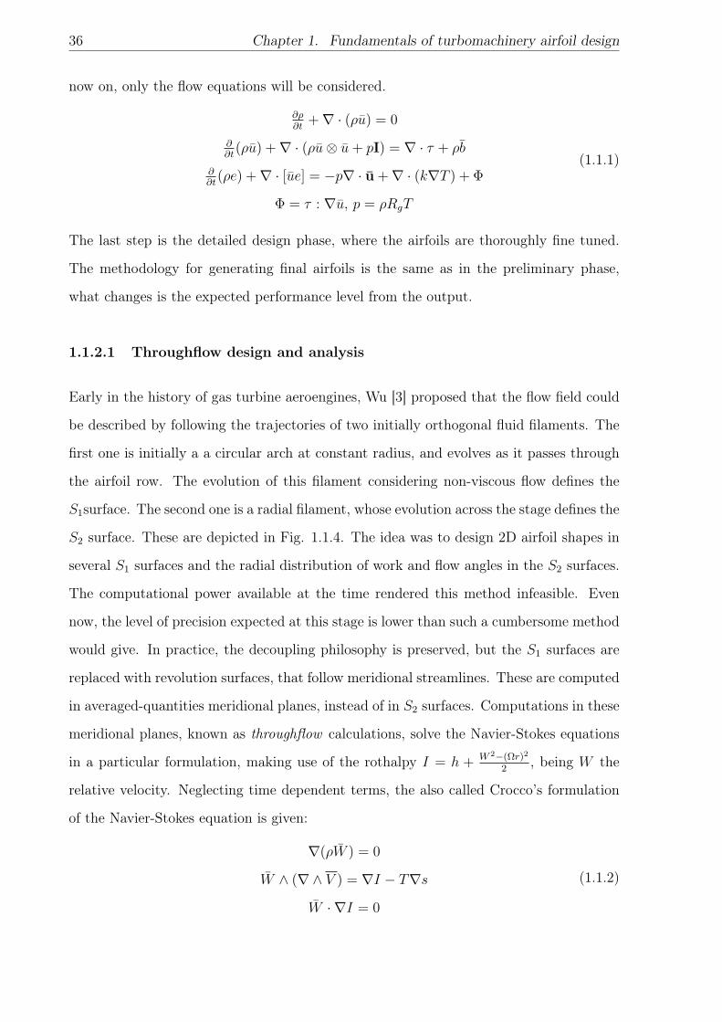
1.1.2.1 Throughflow design and analysis
Early in the history of gas turbine aeroengines, Wu [3] proposed that the flow field could
be described by following the trajectories of two initially orthogonal fluid filaments. The
first one is initially a a circular arch at constant radius, and evolves as it passes through
the airfoil row. The evolution of this filament considering non-viscous flow defines the
S1surface. The second one is a radial filament, whose evolution across the stage defines the
S2 surface. These are depicted in Fig. 1.1.4. The idea was to design 2D airfoil shapes in
several S1 surfaces and the radial distribution of work and flow angles in the S2 surfaces.
The computational power available at the time rendered this method infeasible. Even
now, the level of precision expected at this stage is lower than such a cumbersome method
would give. In practice, the decoupling philosophy is preserved, but the S1 surfaces are
replaced with revolution surfaces, that follow meridional streamlines. These are computed
in averaged-quantities meridional planes, instead of in S2 surfaces. Computations in these
meridional planes, known as throughflow calculations, solve the Navier-Stokes equations
in a particular formulation, making use of the rothalpy I = h + W 2−(Ωr)2
2, being W the
relative velocity. Neglecting time dependent terms, the also called Crocco’s formulation
of the Navier-Stokes equation is given:
∇(ρW ) = 0
W ∧ (∇∧ V ) = ∇I − T∇s
W · ∇I = 0
(1.1.2)
1.1. Generic methodology 37
Figure 1.1.4: Wu’s proposed decoupled surfaces. Source: [3]
Two commonplace solution methods are traditionally described in literature, the
streamline curvature method, and matrix or stream-function methods, although other
possibilities con be considered, such as solving directly the Euler equations as proposed
by Pacciani et al [14]. See [15] for a comprehensive, if early, account of these. Denton
and Dawes [16] prefer the former over the latter, as the stream function method suffers
from solution bifurcation when dealing with transonic flows. Gannon and von Backström
[17] conclude however that the stream function method was more robust and with better
convergence behavior. In practice it comes to the actual implementation strategy, as
neither method is clearly superior. Both methods work by performing a change of
variables. In the streamline curvature method, the coordinates are changed to streamline
coordinates, adding the slope and curvature radius of streamlines to the set of unknowns,
in place of normal velocity, which is zero. The energy equation means in this case that
the rothalpy is convected along the streamline. In the stream function method, a stream
function is posed such that the velocity field is its gradient, and the continuity equation
is automatically fulfilled. A more modern development based on the Euler equations and
modeling the effect of losses, deflections and blockage due to the airfoil row as source
terms is given by Persico and Rebay [18]. During this step of throughflow calculations,
the geometry of the hub and annulus is specified, including mean radius and passage
height variation in the axial direction. Radial distributions of inlet mass-flow, flow angles,
38 Chapter 1. Fundamentals of turbomachinery airfoil design
and outlet flow angles are iterated through by a designer until the required power and
reaction degree is obtained, ensuring that the tangential force distribution in the airfoil
will be uniform and within acceptable bounds, and that losses according to correlations
(basically extensions of the 1D performance correlations) are acceptable.
The output of the process is a set of radial distributions of flow angles and thermodynamic
properties that will serve as boundary conditions for the 2D airfoil design and as a reference
for the results of the high fidelity analysis, and a proposal for radial distribution of axial
chord.
1.1.2.2 Blade to blade design and analysis
In this stage, the 2D airfoil shapes are defined, and the simplified flow field is computed
to check for relevant aerodynamic aspects, such as, loading distribution and boundary
layer development. It is not necessary to model the flow at this stage using very high
fidelity methods, but a relatively high degree of accuracy is required. A common solution
is the use of the Euler equations in a two dimensional plane coupled with a boundary
layer solver, based on the momentum integral equations. Accurate correlations for the
prediction of transition are useful at this stage. The Euler equations are nothing more
than the Navier-Stokes equations neglecting viscous terms.
The definition of geometry is subject to hard constraints, such as manufacturability, or
softer ones, such that the method should ensure a high order of geometrical continuity
(at least G 3). The reason for this will be explained later on, in section 1.2.1, but suffice
to say that curvature discontinuities practically guarantee undesirable flow behavior.
The output of this phase is the geometrical definition of 2D profiles at several span-wise
coordinates, and initial estimations of loading, velocity, and boundary layer thickness
distributions along the profile. Additionally, the prediction of transition location can be
used, if applicable during the high fidelity analysis phase.
1.1.2.3 Three dimensional stacking
The 2D profiles have to be stacked radially in order to generate an actual three dimensional
shape, following what is named the stacking line. In order to define an appropriate
1.1. Generic methodology 39
stacking line, several aspects should be considered. The first consideration is the actual
location of the stacking line with respect to the airfoil. Possible choices are the leading
edge, trailing edge, center of mass, etc... depending on which are the aspects that
the designer wants to have more control over. Stacking rotating blades (rotors) has
its particularities in that structural considerations weigh in earlier than in non rotating
components (stators).
A second aspect is that anything else than a purely radial stacking will introduce pressure
gradients in the plane of deviation. This can be used as a design tool in order to improve
performance, but only if its effects are correctly understood. This issue will be elaborated
on in section 1.2.3.
The final surface definition should also be built with a high order of geometrical continuity,
and needs to be written in a format readily acceptable by the tools which will be
subsequently used for high fidelity analysis.
1.1.2.4 High fidelity analysis and feedback generation
Once a geometry has been defined, its performance must be evaluated to check to which
extent the requirements are met. An initially proposed geometry will be far off from being
satisfactory, so a designer will propose modifications in order to address these deviations
form the objectives, thus closing the design loop. This loop is iterated until a geometry
fulfills all constraints and objectives, or until a deadline is met, whether the result is
completely satisfactory or not. What these objectives are, will be made clear as the
chapter progresses.
Before computing power became an ubiquitous resource, this evaluation was done by
actually building an experimental rig and testing it. The costs (both economical and of
time) of such an approach prevented from a lot of iterations from taking place. Early
gas turbines were inefficient mainly not due to lack of knowledge of designers, but due to
the enormous cost of evaluating candidate geometries. Development in both numerical
methods and computational architectures has been then generally well received, as real
experimentation can be replaced with much cheaper and flexible virtual experimentation.
Well received up to a certain degree, as numerical simulations have some shortcomings
40 Chapter 1. Fundamentals of turbomachinery airfoil design
and accuracy limits that need to be kept in mind. Two sayings that have grown to become
adages illustrate the perils of both blind trust or entrenched skepticism:
• “The greatest disaster one can encounter in computation is not instability or lack of
convergence but results that are simultaneously good enough to be believable but
bad enough to cause trouble.”
• “No one believes the simulation results except the one who performed the
calculation, and everyone believes the experimental results except the one who
performed the experiment.”[19]
The first one advises caution when presented with merely plausible results, and should
remind of the importance of validation against rigorous experimentation. The second one
should remind that real experimentation is also subject to uncertainties, and if these are
not properly quantified, results are rendered suspect.
A high fidelity flow analysis consists therefore of the numerical simulation of the Navier-
Stokes equations in a three dimensional computational domain. The analytic expressions
of these are discretized, that is, translated from a continuous space of independent
variables to a discrete one. But something will always be lost in translation, and the
discrete operators will exhibit a different mathematical behaviour to their continuous
equivalents, something which should be well understood in order to correctly set up a
simulation or interpret the results.
A first step is the preprocessing stage, where a computational domain is defined in terms
of its boundaries and the location of discrete spatial locations or mesh points. Types
of boundary conditions (inlets, outlets, walls, etc...), are also set at this stage. It can
be intuited that the more mesh points for a given domain, the closer the results will be
to the continuum case. While there are finer points to be made regarding the behavior
of discrete operators, this is basically true. On the other hand, simulation time scales
obviously with mesh size. In a design context, a usually stringent upper limit in mesh
size will be imposed in order to achieve reasonable turnaround times. Precision being
limited somewhat by mesh size, an adequate mesh will be smartly designed concentrating
more points in regions with large gradients, and saving them in regions where little is
1.1. Generic methodology 41
happening. This decision can be only because the analyst already has theoretical or
practical knowledge of general flow patterns.
Another resource to limit the expense of a numerical computation is the modeling of non-
resolved scales. In fluid equations this is manifested clearly in the so called Reynolds
Averaged Navier Stokes equations. This formulation uses the technique of ensemble
averaging, borrowed from statistical mechanics, to average out the influence of small
spatial length scales where flow behaves in a chaotic manner. These effects are retained in
the so called Reynolds stress tensor, for which several modeling approaches are possible.
In a classic text on the topic, by Wilcox [20], several turbulence models are proposed,
explaining the underlying hypothesis and range of applicability.
When designing a single airfoil row, it is also common practice to neglect the interaction
with others. This implies that unsteady effects are not resolved, thus making the
simulation much more manageable, but paying a price in terms of accuracy and insight.
Given the mentioned modeling assumptions, one could question the nature of these
simulations as high fidelity. In fact, until computational resources allow for Direct Navier-
Stokes simulations (DNS, no modeling whatsoever) of engineering relevant flows in a
reasonable time frame, this stage is actually the highest fidelity affordable analysis, but
one need not spend so many words. Large Eddy Simulation is an intermediate fidelity
level between RANS and LES, where the largest turbulent scales are resolved, and the
smaller ones are dissipated through a model or a numerical device. While considerably
more affordable than DNS, it still means the simulation of a large number of degrees of
freedom and overrides the validity of steady flow assumptions. Such a simulation is as of
yet not affordable for design purposes.
All these considerations accounted for, the end result is that there is available a piece
of software that provides with a numerical solution to the flow PDEs, which has been
validated against representative simplified test cases. Thus, a measure of the error with
respect to reality should be known when applied to the real design or analysis case.
The resulting flow field is postprocessed, that is, the relevant performance metrics are
qualitatively and quantitatively assessed. Which are these will be explained in the
following section. With this information, the designer knows how much the current
42 Chapter 1. Fundamentals of turbomachinery airfoil design
geometry deviates form requirements and proposes a new one which, according to his
judgment, will fare better in the next iteration. Not only that, but the information from
high fidelity analyses can be used in successive iterations to improve low fidelity ones. For
instance, the entropy related source terms in equation 1.1.2 can be extracted from here,
or the radial angle distribution proposals in the throughflow can follow the general shape
of the one predicted at this stage.
1.2 Aerodynamics of turbomachinery components
As was introduced earlier, what is called a high fidelity analysis in a design context in
practice implies a number of simplifications. Denton [21] provides with a comprehensive
account of these deficiencies. This implies that the difference between real losses and
computed ones will be high enough that the latter cannot be used as a driver for
optimization. Knowledge on the aerodynamics of turbomachines is necessary to posit
adequate performance metrics based on flow features that can be accurately reproduced
by Computational Fluid Dynamics (CFD) simulations.
In this section, the behavior of flows in turbomachinery components is described, so that
it can be understood which are the performance metrics that characterize an airfoil, and
how are they influenced by geometry. Turbomachinery flows are inherently unsteady, due
to the presence of rotating components, and generally turbulent due to high speed free
stream flow. Low Pressure Turbines (LPTs) and Low Pressure Compressors (LPCs)are
components which may operate in a transitional regime, due to the low densities caused
by expansion across the turbine, which will have its implications.
Sources of thermodynamic loss in turbomachines are many. Denton [22] defines loss as
“any flow feature that reduces the efficiency of a turbomachine”. He is however careful
to differentiate between entropy generation mechanisms due to viscous dissipation in
boundary layers, mixing processes, etc... and potential work loss due to vortical features
which may be inviscid in nature. The issue is complicated further, as while this distinction
can be conceptually made, in practice they are coupled and cannot be studied separately.
Instead of giving here an account of possible loss sources, only the aspects that can be
1.2. Aerodynamics of turbomachinery components 43
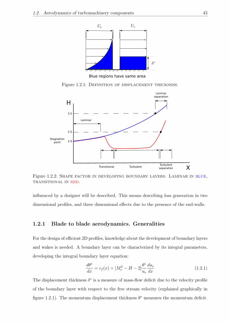
Blue regions have same area
Figure 1.2.1: Definition of displacement thickness.
H
3.5
2.5
2.0
Laminar
Stagnation point
Turbulent
Laminarseparation
TurbulentseparationTransitional X
Figure 1.2.2: Shape factor in developing boundary layers. Laminar in blue,transitional in red.
influenced by a designer will be described. This means describing loss generation in two
dimensional profiles, and three dimensional effects due to the presence of the end-walls.
1.2.1 Blade to blade aerodynamics. Generalities
For the design of efficient 2D profiles, knowledge about the development of boundary layers
and wakes is needed. A boundary layer can be characterized by its integral parameters,
developing the integral boundary layer equation:
dθ∗
dx= cf (x) + [M2
e −H − 2]θ∗
ue
duedx
(1.2.1)
The displacement thickness δ∗ is a measure of mass-flow deficit due to the velocity profile
of the boundary layer with respect to the free stream velocity (explained graphically in
figure 1.2.1). The momentum displacement thickness θ∗ measures the momentum deficit.

44 Chapter 1. Fundamentals of turbomachinery airfoil design
Figure 1.2.3: Friction factor as a function of Reynolds number. Source: [4]
The shape factor H is the ratio between them.
δ∗ =
ˆ ∞0
(1− ρu
ρeue
)dy, θ∗ =
ˆ ∞0
ρu
ρeue
(1− u
ue
)dy, H =
δ∗
θ∗
In figure 1.2.2, it is depicted how the shape factor varies in a developing boundary layer
for both laminar and turbulent cases, including critical values where separation takes
place. Laminar shape factors are higher than turbulent ones, meaning that laminar
boundary layers lose more momentum. This renders them more sensitive to adverse
pressure gradients, and as such, more prone to separation. The following equation relates
θ∗ to the friction coefficient cf = τ/12ρu2, free stream stream-wise velocity gradients
due/dx, free stream Mach number Me, and boundary layer shape factor H. Finally, the
auxiliary equation, closes the system, coupling H with the terms in equation 1.2.1.
θ∗dH
dx= F
(H, θ∗,
θ∗
ue
duedx
)(1.2.2)
Thompson [23] reviews a number of empirical correlations used to model the auxiliary
equation.
In figure 1.2.3, cf is plotted against Reynolds number. It is seen how for laminar regimes,
cf decreases exponentially with Re. For turbulent regimes, it becomes independent of Re,
but very dependent on surface roughness. It must be noted that this diagram was initially
devised for piping applications, where manufacturing tolerances may allow high roughness
measured in boundary layer units. In turbomachinery applications, it is commonplace to
achieve such manufacturing standards, that roughness is below the hydraulically smooth
threshold. Below this critical height, roughness peaks are immersed in the laminar
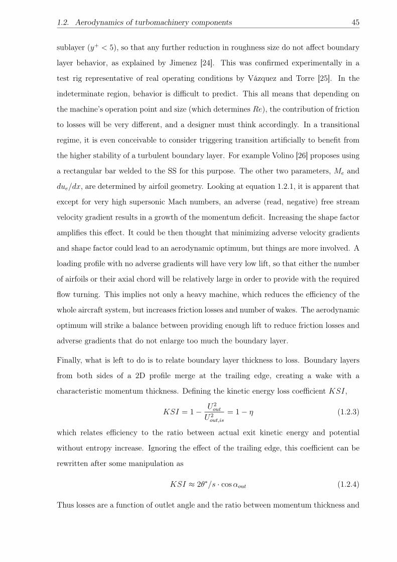
1.2. Aerodynamics of turbomachinery components 45
sublayer (y+ < 5), so that any further reduction in roughness size do not affect boundary
layer behavior, as explained by Jimenez [24]. This was confirmed experimentally in a
test rig representative of real operating conditions by Vázquez and Torre [25]. In the
indeterminate region, behavior is difficult to predict. This all means that depending on
the machine’s operation point and size (which determines Re), the contribution of friction
to losses will be very different, and a designer must think accordingly. In a transitional
regime, it is even conceivable to consider triggering transition artificially to benefit from
the higher stability of a turbulent boundary layer. For example Volino [26] proposes using
a rectangular bar welded to the SS for this purpose. The other two parameters, Me and
due/dx, are determined by airfoil geometry. Looking at equation 1.2.1, it is apparent that
except for very high supersonic Mach numbers, an adverse (read, negative) free stream
velocity gradient results in a growth of the momentum deficit. Increasing the shape factor
amplifies this effect. It could be then thought that minimizing adverse velocity gradients
and shape factor could lead to an aerodynamic optimum, but things are more involved. A
loading profile with no adverse gradients will have very low lift, so that either the number
of airfoils or their axial chord will be relatively large in order to provide with the required
flow turning. This implies not only a heavy machine, which reduces the efficiency of the
whole aircraft system, but increases friction losses and number of wakes. The aerodynamic
optimum will strike a balance between providing enough lift to reduce friction losses and
adverse gradients that do not enlarge too much the boundary layer.
Finally, what is left to do is to relate boundary layer thickness to loss. Boundary layers
from both sides of a 2D profile merge at the trailing edge, creating a wake with a
characteristic momentum thickness. Defining the kinetic energy loss coefficient KSI,
KSI = 1− U2out
U2out,is
= 1− η (1.2.3)
which relates efficiency to the ratio between actual exit kinetic energy and potential
without entropy increase. Ignoring the effect of the trailing edge, this coefficient can be
rewritten after some manipulation as
KSI ≈ 2θ∗/s · cosαout (1.2.4)
Thus losses are a function of outlet angle and the ratio between momentum thickness and
46 Chapter 1. Fundamentals of turbomachinery airfoil design
pitch θ∗/s. In these analyses pertaining the thickness of the boundary layer, there is a
term which has not yet been addressed, the free stream velocity ue. The steady, inviscid,
2D momentum equations in streamline coordinates are:
ρV∂V
∂s= −∂p
∂s
ρV 2
R=∂p
∂n
(1.2.5)
Considering ue = V , the equation in the stream aligned direction establishes the
relationship between free stream velocity and pressure gradient. The equation in the
normal direction relates the pressure gradient to velocity and curvature radius. In order
to generate continuous velocity distributions, it is necessary to have continuous curvature
distributions. In addition, a curvature discontinuity con potentially result in a pressure
gradient that can qualitatively alter the state of the boundary layer.
1.2.2 Secondary flows. Generalities
Regarding three dimensional effects, due to the presence of the end-walls, the so called
secondary flows appear. Several flow features have been described in literature, for
example by Sieverding [27], or Wennerstrom [28], but in the following, only those over
which a designer could have more control are described.
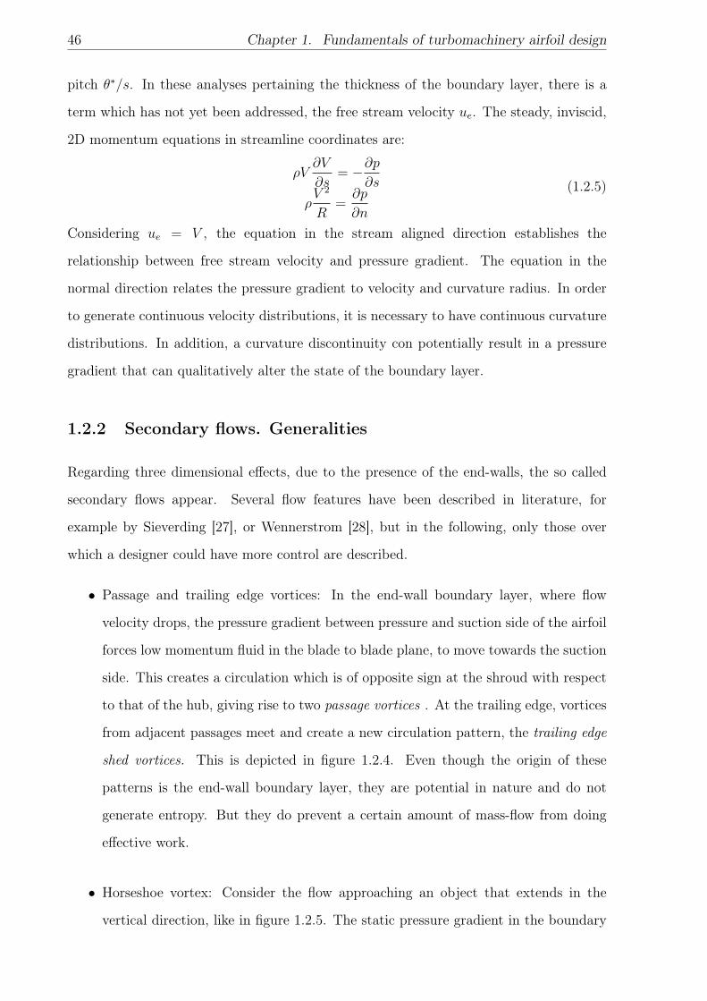
• Passage and trailing edge vortices: In the end-wall boundary layer, where flow
velocity drops, the pressure gradient between pressure and suction side of the airfoil
forces low momentum fluid in the blade to blade plane, to move towards the suction
side. This creates a circulation which is of opposite sign at the shroud with respect
to that of the hub, giving rise to two passage vortices . At the trailing edge, vortices
from adjacent passages meet and create a new circulation pattern, the trailing edge
shed vortices. This is depicted in figure 1.2.4. Even though the origin of these
patterns is the end-wall boundary layer, they are potential in nature and do not
generate entropy. But they do prevent a certain amount of mass-flow from doing
effective work.
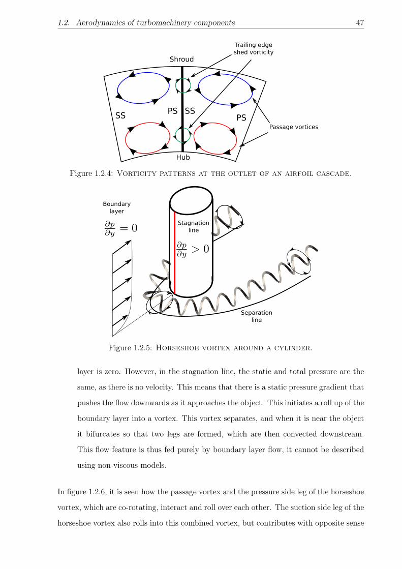
• Horseshoe vortex: Consider the flow approaching an object that extends in the
vertical direction, like in figure 1.2.5. The static pressure gradient in the boundary
1.2. Aerodynamics of turbomachinery components 47
SS PS
Hub
Shroud
SSPS
Passage vortices
Trailing edge shed vorticity
Figure 1.2.4: Vorticity patterns at the outlet of an airfoil cascade.
Stagnation line
Boundary layer
Separation line
Figure 1.2.5: Horseshoe vortex around a cylinder.
layer is zero. However, in the stagnation line, the static and total pressure are the
same, as there is no velocity. This means that there is a static pressure gradient that
pushes the flow downwards as it approaches the object. This initiates a roll up of the
boundary layer into a vortex. This vortex separates, and when it is near the object
it bifurcates so that two legs are formed, which are then convected downstream.
This flow feature is thus fed purely by boundary layer flow, it cannot be described
using non-viscous models.
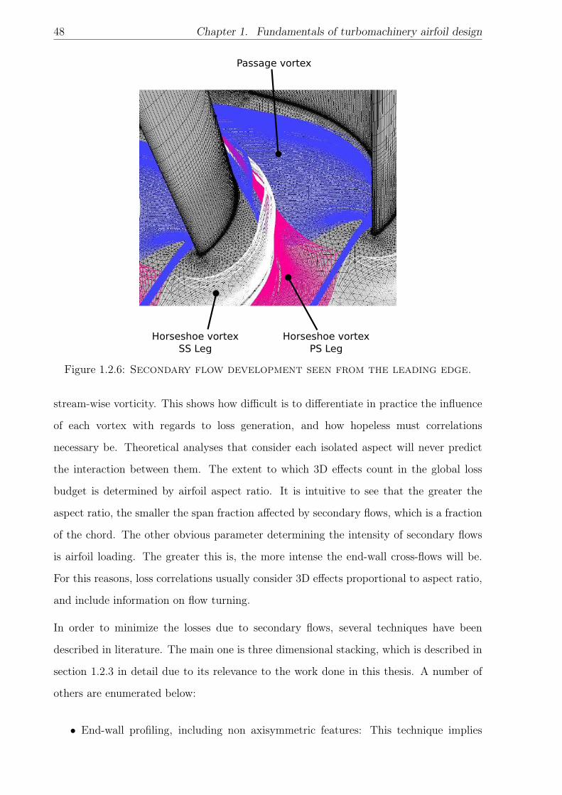
In figure 1.2.6, it is seen how the passage vortex and the pressure side leg of the horseshoe
vortex, which are co-rotating, interact and roll over each other. The suction side leg of the
horseshoe vortex also rolls into this combined vortex, but contributes with opposite sense
48 Chapter 1. Fundamentals of turbomachinery airfoil design
Passage vortex
Horseshoe vortexSS Leg
Horseshoe vortexPS Leg
Figure 1.2.6: Secondary flow development seen from the leading edge.
stream-wise vorticity. This shows how difficult is to differentiate in practice the influence
of each vortex with regards to loss generation, and how hopeless must correlations
necessary be. Theoretical analyses that consider each isolated aspect will never predict
the interaction between them. The extent to which 3D effects count in the global loss
budget is determined by airfoil aspect ratio. It is intuitive to see that the greater the
aspect ratio, the smaller the span fraction affected by secondary flows, which is a fraction
of the chord. The other obvious parameter determining the intensity of secondary flows
is airfoil loading. The greater this is, the more intense the end-wall cross-flows will be.
For this reasons, loss correlations usually consider 3D effects proportional to aspect ratio,
and include information on flow turning.
In order to minimize the losses due to secondary flows, several techniques have been
described in literature. The main one is three dimensional stacking, which is described in
section 1.2.3 in detail due to its relevance to the work done in this thesis. A number of
others are enumerated below:
• End-wall profiling, including non axisymmetric features: This technique implies

1.2. Aerodynamics of turbomachinery components 49
application of a complex curvature distribution for the definition of end-wall
geometry. If only applied in the meridional plane, it is referred to as end-wall
contouring or end-wall profiling. If applied also in the tangential plane, it is called
non-axisymmetric end-wall design. The aim is to induce localized pressure gradients
to redirect mass-flow or counteract the motion of secondary flows. Experimental
studies of this concept have been done by Duden et al [29], regarding the effects
of contouring only in the meridional plane. Regarding non-axisymmetric end-walls,
Torre et al [30] performed a numerical study based on geometries proposed by
engineering judgment, and Corral and Gisbert [31] used automatic design techniques
to generate the optimal geometries.
• Fences: Initially proposed by Prümper [32], a fence is meant to act as a physical
barrier to confine separated flow within a region. An important parameter is the
depth of immersion of the fence within the main flow. Kumar and Govardhan [33]
experiment with an axially varying height to account for boundary layer growth.
The main problem with such a device is the additional flow features generated due
to its presence, which are very difficult to control by design.
• Leading edge modifications: The intensity horseshoe vortex is heavily influenced by
LE geometry. Recalling that the passage vortex rotates in the opposite sense to that
of the SS side leg of the horseshoe vortex, Sauer et al [34] proposed intensifying the
latter with an increased LE radius in the end-wall region, so that it weakens the
former.
• Swirl generators: The concept is similar to that of LE modifications, that is, to
counteract secondary flows vorticity with vorticity in the opposite sense. Lei et al
[35] propose to use vortex generators at the beginning of the blade passage for this
purpose.
All these techniques have not found their place in real world applications mainly due
to their poor performance in off design conditions, and the lack of reliable and trusted
analysis tools for these configurations. Their principle of operation depends on the fine
tuning of very specific flow features, which in a real machine are bound to be very variable.
50 Chapter 1. Fundamentals of turbomachinery airfoil design
1.2.3 Three dimensional design techniques
Airfoils can be stacked leaning in the axial and tangential directions. The intention is to
create pressure gradients in the meridional and normal planes, which may help redistribute
mass-flow, counteract non desirable radial pressure gradients due a to non homogeneous
lift distribution, or contain separated flow preventing its dispersion and mixing with the
main flow. Axial lean is also known as sweep, and tangential lean as dihedral, in analogy
to the same design features in wings. Lewis and Hill [36] present an analytical approach
to the description of these effects. They are able to predict the new blade loading in the
blade-to-blade plane taking into consideration that the leaning movement in both planes
changes the stream surface, and describe how the throughflow equations can be modified
to account for these effects.
Sweep may appear naturally in turbomachines with hade angle (the angle between the
horizontal and the end-wall contour in the meridional plane) when the decision is made
to stack airfoils radially. The reason for this is mainly the reduction of root moments in
rotors, but also in order to reduce machine length. Pullan and Harvey [37] argue that a
swept profile will always have greater 2D losses than an identically loaded un-swept one.
In an accompanying work [38] they study the effects of sweep in the end-wall regions, and
how the sweep induced pressure gradients affect the loading of the near end-wall profiles.
In the uniform sweep geometry they present, secondary losses penetration is contained at
hub but exacerbated at the shroud.
It should be always kept in mind that separation between 2D and 3D effects is an
abstraction to ease the design process, but in reality, that decoupling does not exist. In
order to take advantage of airfoil leaning, or minimize its effects when it is not desirable
but unavoidable, 2D profile shapes must be considered concurrently.
1.2.4 Unsteady effects. Generalities
Flows in turbomachinery are obviously unsteady due to the presence of rotating parts and
high Re numbers. However, the analysis methods spoken of so far all make the assumption
of steady flow. Retaining the effect of unsteadiness adds a level of computational cost that,

1.2. Aerodynamics of turbomachinery components 51
Figure 1.2.7: Wakes across blade rows.
in the current state of the art, is not acceptable within a design environment. Thus, the
effects of unsteadiness are studied in advance, conclusions are extracted, and translated
into additional design rules. The most relevant issues to consider at this stage are the
following:
Incoming wake interaction: In an airfoil row, the wakes of a preceding one enter the
passage and impact the airfoils at varying locations due to the relative motion between
the two rows (see figure 1.2.7). The impingement of wakes in a laminar developing
boundary layer will modify its behaviour, creating transitional/turbulent strips of flow.
This can be either through the mechanism of bypass transition, for attached flow, or
through the breakdown of the Kelvin-Helmholtz instability in shear layers, for separated
flow transition. Regions of calmed flow usually trail these strips as they move over the
blade surface. The calmed regions are initially associated with a full-velocity profile and
therefore a high wall shear stress that then relaxes back to a laminar value. While the
transitional/turbulent strips tend to increase losses, the calmed regions tend to reduce
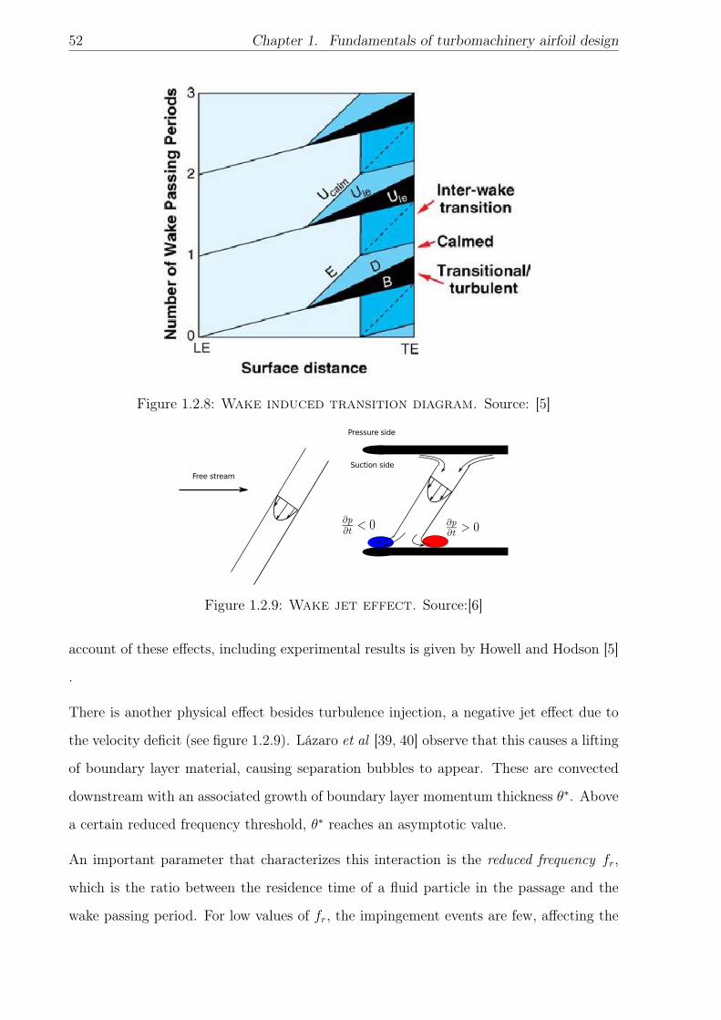
losses compared to the undisturbed boundary layer. Figure 1.2.8 shows an sketch of the a
generic suction side affected by wake passing, whre the convection of these trubulent strips
is plotted, including the calmed flow region (light blus) and turbulent flow due to wake
induced transition (black) and undisturbed flow transition (dark blue). A comprehensive
52 Chapter 1. Fundamentals of turbomachinery airfoil design
Figure 1.2.8: Wake induced transition diagram. Source: [5]
Figure 1.2.9: Wake jet effect. Source:[6]
account of these effects, including experimental results is given by Howell and Hodson [5]
.
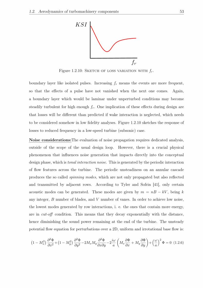
There is another physical effect besides turbulence injection, a negative jet effect due to
the velocity deficit (see figure 1.2.9). Lázaro et al [39, 40] observe that this causes a lifting
of boundary layer material, causing separation bubbles to appear. These are convected
downstream with an associated growth of boundary layer momentum thickness θ∗. Above
a certain reduced frequency threshold, θ∗ reaches an asymptotic value.
An important parameter that characterizes this interaction is the reduced frequency fr,
which is the ratio between the residence time of a fluid particle in the passage and the
wake passing period. For low values of fr, the impingement events are few, affecting the
1.2. Aerodynamics of turbomachinery components 53
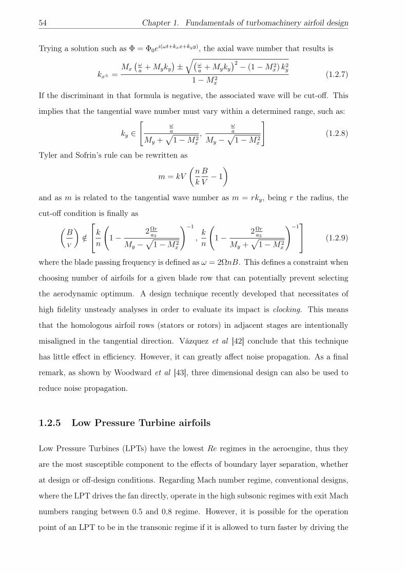
Figure 1.2.10: Sketch of loss variation with fr.
boundary layer like isolated pulses. Increasing fr means the events are more frequent,
so that the effects of a pulse have not vanished when the next one comes. Again,
a boundary layer which would be laminar under unperturbed conditions may become
steadily turbulent for high enough fr. One implication of these effects during design are
that losses will be different than predicted if wake interaction is neglected, which needs
to be considered somehow in low fidelity analyses. Figure 1.2.10 sketches the response of
losses to reduced frequency in a low-speed turbine (subsonic) case.
Noise considerations:The evaluation of noise propagation requires dedicated analysis,
outside of the scope of the usual design loop. However, there is a crucial physical
phenomenon that influences noise generation that impacts directly into the conceptual
design phase, which is tonal interaction noise. This is generated by the periodic interaction
of flow features across the turbine. The periodic unsteadiness on an annular cascade
produces the so called spinning modes, which are not only propagated but also reflected
and transmitted by adjacent rows. According to Tyler and Sofrin [41], only certain
acoustic modes can be generated. These modes are given by m = nB − kV , being k
any integer, B number of blades, and V number of vanes. In order to achieve low noise,
the lowest modes generated by row interactions, i. e. the ones that contain more energy,
are in cut-off condition. This means that they decay exponentially with the distance,
hence diminishing the sound power remaining at the end of the turbine. The unsteady
potential flow equation for perturbations over a 2D, uniform and irrotational base flow is:
(1−M2
x
) ∂2Φ
∂x2+(1−M2
y
) ∂2Φ
∂y2−2MxMy
∂2Φ
∂x∂y−2
iω
a
(Mx
∂Φ
∂x+ My
∂Φ
∂y
)+(ωa
)2Φ = 0 (1.2.6)
54 Chapter 1. Fundamentals of turbomachinery airfoil design
Trying a solution such as Φ = Φ0ei(ωt+kxx+kyy), the axial wave number that results is
kx± =Mx
(ωa
+Myky)±√(
ωa
+Myky)2 − (1−M2
x) k2y
1−M2x
(1.2.7)
If the discriminant in that formula is negative, the associated wave will be cut-off. This
implies that the tangential wave number must vary within a determined range, such as:
ky ∈
[ωa
My +√
1−M2x
,ωa
My −√
1−M2x
](1.2.8)
Tyler and Sofrin’s rule can be rewritten as
m = kV
(n
k
B
V− 1
)and as m is related to the tangential wave number as m = rky, being r the radius, the
cut-off condition is finally as(B
V
)/∈
kn
(1−
2Ωra3
My −√
1−M2x
)−1
,k
n
(1−
2Ωra3
My +√
1−M2x
)−1 (1.2.9)
where the blade passing frequency is defined as ω = 2ΩnB. This defines a constraint when
choosing number of airfoils for a given blade row that can potentially prevent selecting
the aerodynamic optimum. A design technique recently developed that necessitates of
high fidelity unsteady analyses in order to evaluate its impact is clocking. This means
that the homologous airfoil rows (stators or rotors) in adjacent stages are intentionally
misaligned in the tangential direction. Vázquez et al [42] conclude that this technique
has little effect in efficiency. However, it can greatly affect noise propagation. As a final
remark, as shown by Woodward et al [43], three dimensional design can also be used to
reduce noise propagation.
1.2.5 Low Pressure Turbine airfoils
Low Pressure Turbines (LPTs) have the lowest Re regimes in the aeroengine, thus they
are the most susceptible component to the effects of boundary layer separation, whether
at design or off-design conditions. Regarding Mach number regime, conventional designs,
where the LPT drives the fan directly, operate in the high subsonic regimes with exit Mach
numbers ranging between 0.5 and 0,8 regime. However, it is possible for the operation
point of an LPT to be in the transonic regime if it is allowed to turn faster by driving the
1.2. Aerodynamics of turbomachinery components 55
fan through a gearbox. This tends to decrease the loading coefficient ψ, and can be used
reduce the number of stages if ψ is forced to remain constant. There is scarce literature
published in high rotational speed l LPT design, as this technology is the current state
of the art, or in development phase for most companies. In the following, only aspects
related to low rotational speed airfoil design are mentioned.
Recalling section 1.2.1, there is an aerodynamically optimum pitch to chord ratio. This
is seldom selected, since considering whole system efficiency, it is preferable to reduce
machine weight. This is done by reducing the number of airfoils, thus increasing the
pitch. Figure 1.2.11 shows the effect of such a design philosophy in blade loading. It is
evident the increase in adverse pressure gradient after the peak value for the increased lift
case. This would immediately result in higher losses and more susceptibility to boundary
layer separation, rendering the design a more challenging endeavor. A possible solution
to reduce the pressure gradient, is to move the pressure peak forward. For a given total
loading value, a more front loaded airfoil will have lower gradient than an aft loaded one
(see figure 1.2.12). While the risk of separation is mitigated, the amount of boundary
layer material subject to adverse pressure gradient is higher, resulting in higher losses.
Depending on the actual Re value, optimal peak location may vary. Coull et al [44],
provide with empirical evidence of the effects of peak value position, with experiments on
a flat plate subject to pressure gradients that simulate real LPT loadings. Zoric et al [45],
reach the same conclusions using actual LPT profiles measured in linear cascades, adding
that front loaded shapes may cause more intense cross-flows in the end-wall boundary
layers, thus energizing the passage vortices. But additional factors need to be considered
when designing a loading shape. A real machine will be operating a non-negligible part
of its mission at off design conditions. This translates to inflow with positive or negative
incidences. Negative incidences are associated with a loading level decrease. Loss in
machine performance is due to less work being done, as thermodynamic losses are actually
reduced. Positive incidences lead to increased loading levels. Zoric et al [46] conclude
that for the relatively small positive incidences they tested, front loaded airfoils behave
better. However, for even higher positive incidences, it may be that the flow separates
in the vicinity of the LE. In order to reduce the risk of this happening, the peak value
may be placed closer to the rear part. Given the complexity of the whole issue, deciding
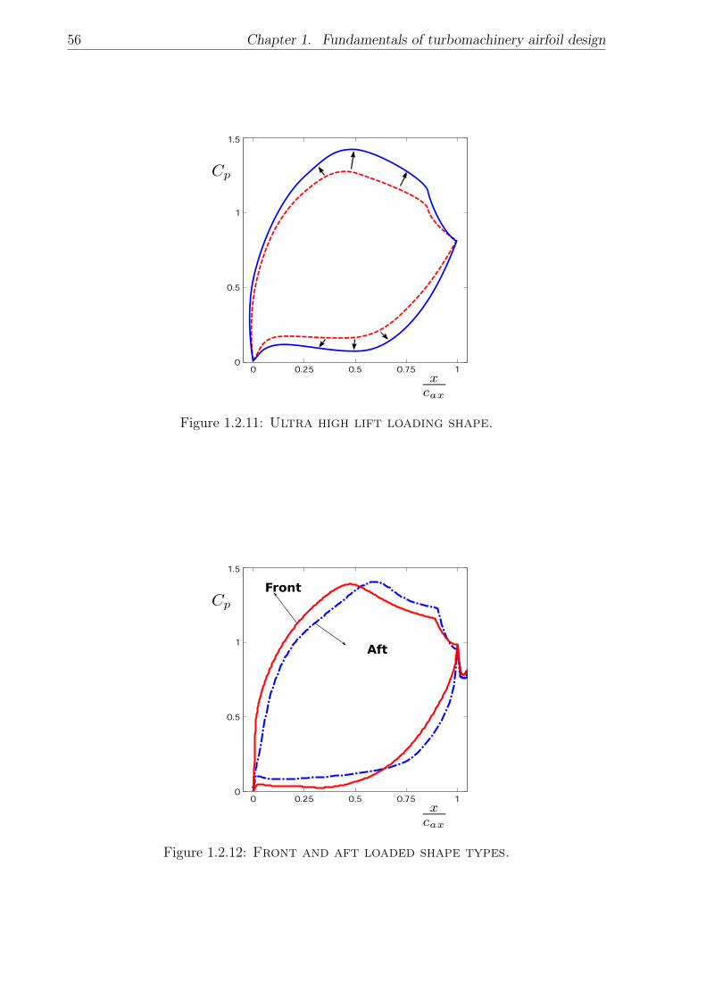
56 Chapter 1. Fundamentals of turbomachinery airfoil design
Figure 1.2.11: Ultra high lift loading shape.
Front
Aft
Figure 1.2.12: Front and aft loaded shape types.

1.2. Aerodynamics of turbomachinery components 57
Figure 1.2.13: LPT profile types. Left, thick. Right, Thin.
over loading level and shape (for design and off design conditions) is not a decision of
the designer. It is the output of R&D campaigns, and a designer’s job is to produce the
geometry that fulfills a set of given design criteria.
This discussion over loading shape was concerned with the suction side. Pressure side
loading is determined largely by airfoil thickness. Depending on design philosophy, three
pressure side types can be described. A thick airfoil (figure 1.2.13, left) will in general
have an attached boundary layer. This type of airfoil is very heavy, so it is usually built
hollow. As it can be expected, this leads to a costly manufacturing process. In order
to reduce manufacturing complexity, a thin airfoil (figure 1.2.13, right) can be designed.
As the flow decelerates just after the LE, it is possible that it separates and creates a
pressure side recirculation bubble. Torre et al [47] found that this recirculation bubble
does not lead necessarily to higher losses at design point. At off design a performance
drop was noted, but due to increased blockage, not directly to loss increase. There
is however another issue. This low momentum material is more susceptible to radial
pressure gradients (such as those due to secondary flows), which may cause it to migrate
radially. Thus, these authors conclude that for near end-wall profiles, the recirculation
bubble should be avoided. A final possibility is to have thin airfoils, designed to avoid
the recirculation bubble. According to what has been mentioned, this choice cannot be
due to efficiency concerns, but it is a way to increase total loading. For a designer, this
means that a radial thickness distribution is a requirement fixed by a lead engineer who
has decided upon the design philosophy to be followed in a certain project.
The previous discussion has to be completed with a review of the implications of a
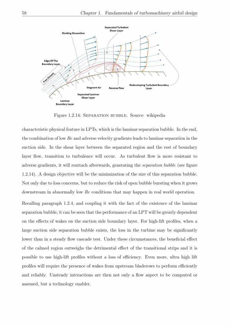
58 Chapter 1. Fundamentals of turbomachinery airfoil design
Figure 1.2.14: Separation bubble. Source: wikipedia
characteristic physical feature in LPTs, which is the laminar separation bubble. In the end,
the combination of lowRe and adverse velocity gradients leads to laminar separation in the
suction side. In the shear layer between the separated region and the rest of boundary
layer flow, transition to turbulence will occur. As turbulent flow is more resistant to
adverse gradients, it will reattach afterwards, generating the separation bubble (see figure
1.2.14). A design objective will be the minimization of the size of this separation bubble.
Not only due to loss concerns, but to reduce the risk of open bubble bursting when it grows
downstream in abnormally low Re conditions that may happen in real world operation.
Recalling paragraph 1.2.4, and coupling it with the fact of the existence of the laminar
separation bubble, it can be seen that the performance of an LPT will be greatly dependent
on the effects of wakes on the suction side boundary layer. For high-lift profiles, when a
large suction side separation bubble exists, the loss in the turbine may be significantly
lower than in a steady flow cascade test. Under these circumstances, the beneficial effect
of the calmed region outweighs the detrimental effect of the transitional strips and it is
possible to use high-lift profiles without a loss of efficiency. Even more, ultra high lift
profiles will require the presence of wakes from upstream bladerows to perform efficiently
and reliably. Unsteady interactions are then not only a flow aspect to be computed or
assessed, but a technology enabler.
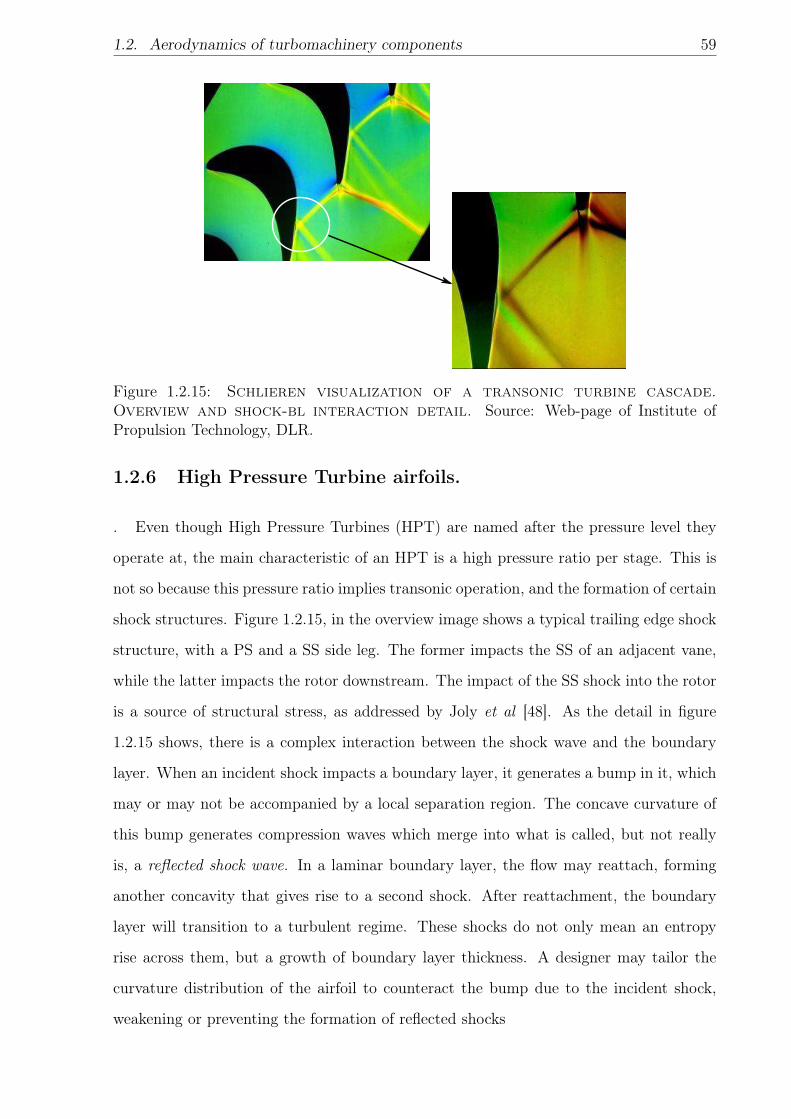
1.2. Aerodynamics of turbomachinery components 59
Figure 1.2.15: Schlieren visualization of a transonic turbine cascade.Overview and shock-bl interaction detail. Source: Web-page of Institute ofPropulsion Technology, DLR.
1.2.6 High Pressure Turbine airfoils.
. Even though High Pressure Turbines (HPT) are named after the pressure level they
operate at, the main characteristic of an HPT is a high pressure ratio per stage. This is
not so because this pressure ratio implies transonic operation, and the formation of certain
shock structures. Figure 1.2.15, in the overview image shows a typical trailing edge shock
structure, with a PS and a SS side leg. The former impacts the SS of an adjacent vane,
while the latter impacts the rotor downstream. The impact of the SS shock into the rotor
is a source of structural stress, as addressed by Joly et al [48]. As the detail in figure
1.2.15 shows, there is a complex interaction between the shock wave and the boundary
layer. When an incident shock impacts a boundary layer, it generates a bump in it, which
may or may not be accompanied by a local separation region. The concave curvature of
this bump generates compression waves which merge into what is called, but not really
is, a reflected shock wave. In a laminar boundary layer, the flow may reattach, forming
another concavity that gives rise to a second shock. After reattachment, the boundary
layer will transition to a turbulent regime. These shocks do not only mean an entropy
rise across them, but a growth of boundary layer thickness. A designer may tailor the
curvature distribution of the airfoil to counteract the bump due to the incident shock,
weakening or preventing the formation of reflected shocks
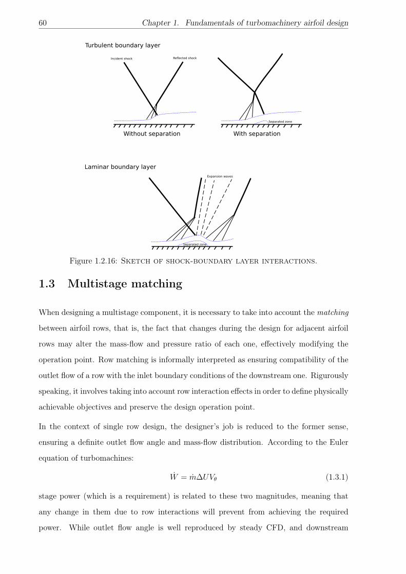
60 Chapter 1. Fundamentals of turbomachinery airfoil design
Incident shock Reflected shock
Without separation With separation
Separated zone
Expansion waves
Separated zone
Turbulent boundary layer
Laminar boundary layer
Figure 1.2.16: Sketch of shock-boundary layer interactions.
1.3 Multistage matching
When designing a multistage component, it is necessary to take into account the matching
between airfoil rows, that is, the fact that changes during the design for adjacent airfoil
rows may alter the mass-flow and pressure ratio of each one, effectively modifying the
operation point. Row matching is informally interpreted as ensuring compatibility of the
outlet flow of a row with the inlet boundary conditions of the downstream one. Rigurously
speaking, it involves taking into account row interaction effects in order to define physically
achievable objectives and preserve the design operation point.
In the context of single row design, the designer’s job is reduced to the former sense,
ensuring a definite outlet flow angle and mass-flow distribution. According to the Euler
equation of turbomachines:
W = m∆UVθ (1.3.1)
stage power (which is a requirement) is related to these two magnitudes, meaning that
any change in them due to row interactions will prevent from achieving the required
power. While outlet flow angle is well reproduced by steady CFD, and downstream
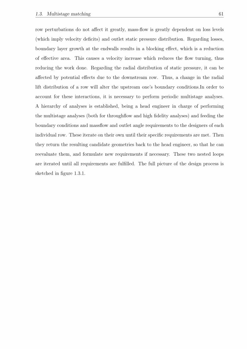
1.3. Multistage matching 61
row perturbations do not affect it greatly, mass-flow is greatly dependent on loss levels
(which imply velocity deficits) and outlet static pressure distribution. Regarding losses,
boundary layer growth at the endwalls results in a blocking effect, which is a reduction
of effective area. This causes a velocity increase which reduces the flow turning, thus
reducing the work done. Regarding the radial distribution of static pressure, it can be
affected by potential effects due to the downstream row. Thus, a change in the radial
lift distribution of a row will alter the upstream one’s boundary conditions.In order to
account for these interactions, it is necessary to perform periodic multistage analyses.
A hierarchy of analyses is established, being a head engineer in charge of performing
the multistage analyses (both for throughflow and high fidelity analyses) and feeding the
boundary conditions and massflow and outlet angle requirements to the designers of each
individual row. These iterate on their own until their specific requirements are met. Then
they return the resulting candidate geometries back to the head engineer, so that he can
reevaluate them, and formulate new requirements if necessary. These two nested loops
are iterated until all requirements are fulfilled. The full picture of the design process is
sketched in figure 1.3.1.
62 Chapter 1. Fundamentals of turbomachinery airfoil design
Conceptual design(1D meanline)
Multirow throughflow
Multirow CFD
Single row throughflow
Single row CFD
Blade to blade design
Yes
NoMeets criteria?
Meets criteria?
Yes
No
Accept
.
.
.
.
.
.
Figure 1.3.1: Multirow workflow.
Chapter 2
Optimization methods
The design problem will be formulated as a multiobjective constrained optimization
problem, in order to use a mathematical algorithm to solve it. In this chapter a broad
overview of the different classes of methods described in literature is given, and the finally
chosen option is described. Such an optimization problem is defined as the search of a
design vector α, such that the objective functions are minimized, while satisfying some
constraints. These may restrict the design space by directly imposing boundaries on
the design vector, or because some performance metric is not acceptable, giving rise to
inequality constraints. Equality constraints arise when some performance requirement
is to be exactly matched, having the effect of reducing the dimensionality of the design
space. A generic optimization problem can then be formulated as:
Minimize fi(α) i = 1, N (2.0.1)
Subject to gj(α) ≤ 0 j = 1, P
hk(α) = 0 k = 1, Q
αlp(α) ≤ αp ≤ αup(α) p = 1, R
One important concept is that of dominance. In figure 2.0.1, design C is clearly dominated
by B, as it is worse performing in both metrics f1 and f2. Compared to A, however, C is
better at f2 but much worse at f1. It is possible to find designs which perform as well as
C at f2 but better at f1. When improvement at one objective cannot be achieved without
sacrificing the other, the design is non-dominated. Collecting the set of non-dominated
63
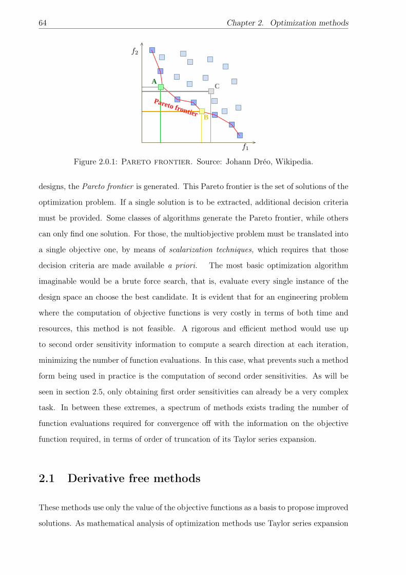
64 Chapter 2. Optimization methods
CA
B
Pareto frontier
Figure 2.0.1: Pareto frontier. Source: Johann Dréo, Wikipedia.
designs, the Pareto frontier is generated. This Pareto frontier is the set of solutions of the
optimization problem. If a single solution is to be extracted, additional decision criteria
must be provided. Some classes of algorithms generate the Pareto frontier, while others
can only find one solution. For those, the multiobjective problem must be translated into
a single objective one, by means of scalarization techniques, which requires that those
decision criteria are made available a priori. The most basic optimization algorithm
imaginable would be a brute force search, that is, evaluate every single instance of the
design space an choose the best candidate. It is evident that for an engineering problem
where the computation of objective functions is very costly in terms of both time and
resources, this method is not feasible. A rigorous and efficient method would use up
to second order sensitivity information to compute a search direction at each iteration,
minimizing the number of function evaluations. In this case, what prevents such a method
form being used in practice is the computation of second order sensitivities. As will be
seen in section 2.5, only obtaining first order sensitivities can already be a very complex
task. In between these extremes, a spectrum of methods exists trading the number of
function evaluations required for convergence off with the information on the objective
function required, in terms of order of truncation of its Taylor series expansion.
2.1 Derivative free methods
These methods use only the value of the objective functions as a basis to propose improved
solutions. As mathematical analysis of optimization methods use Taylor series expansion
2.1. Derivative free methods 65
to prove convergence theorems, it follows that these methods are not guaranteed to
converge to the optimum solution, and if they do, the number of iterations cannot be
estimated. In practice, there are real world applications where their performance is
good enough, and even some, for example when the objective functions are noisy or
discontinuous, where these are the only methods that can be used. Their formulation is
based on heuristics, which can often be analogies with natural physical processes.
2.1.1 Population based methods
These algorithms use an initial set of solutions to combine their features in order to propose
improved ones, thus modifying that initial population. Using appropriate methods for
ranking each individual in the population, the full Pareto frontier can be generated. Two
of the most used classes are described in the following.
• Evolutionary strategies.
Algorithms belonging to this class are modeled after some simple ideas of live
organisms evolution. The design vector represents the genotype, and population
variation is guided by some specified models of gene recombination between
individuals. Introducing random variations, or mutations, in the gene recombination
procedure, these methods cease to be deterministic, and they are able to find
global optima regardless of the composition of the initial population. A new set
of individuals is generated and evaluated, and a new population is built discarding
unfit individuals through a selection process. Thus populations evolve, and the
process is converged when a population is clustered in such a way that the Pareto
front is discernible (if a multi-objective discerning selection is used) or around a
single point (in a single objective problem). Given that no mathematical proof
of convergence can be posited, convergence is assumed when populations cease to
evolve meaningfully.
Many selection operators have been described in literature, and new proposals
appear regularly. Blickle and Tiele [49] provide with a review of several schemes
used in single objective applications. For an account on multiple objective ones, see
Konak et al [50].
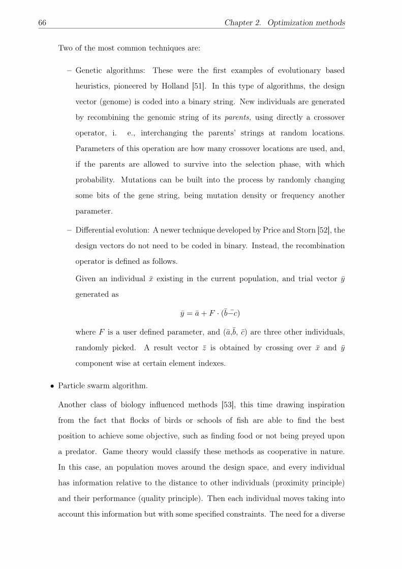
66 Chapter 2. Optimization methods
Two of the most common techniques are:
– Genetic algorithms: These were the first examples of evolutionary based
heuristics, pioneered by Holland [51]. In this type of algorithms, the design
vector (genome) is coded into a binary string. New individuals are generated
by recombining the genomic string of its parents, using directly a crossover
operator, i. e., interchanging the parents’ strings at random locations.
Parameters of this operation are how many crossover locations are used, and,
if the parents are allowed to survive into the selection phase, with which
probability. Mutations can be built into the process by randomly changing
some bits of the gene string, being mutation density or frequency another
parameter.
– Differential evolution: A newer technique developed by Price and Storn [52], the
design vectors do not need to be coded in binary. Instead, the recombination
operator is defined as follows.
Given an individual x existing in the current population, and trial vector y
generated as
y = a+ F · (b−c)
where F is a user defined parameter, and (a,b, c) are three other individuals,
randomly picked. A result vector z is obtained by crossing over x and y
component wise at certain element indexes.
• Particle swarm algorithm.
Another class of biology influenced methods [53], this time drawing inspiration
from the fact that flocks of birds or schools of fish are able to find the best
position to achieve some objective, such as finding food or not being preyed upon
a predator. Game theory would classify these methods as cooperative in nature.
In this case, an population moves around the design space, and every individual
has information relative to the distance to other individuals (proximity principle)
and their performance (quality principle). Then each individual moves taking into
account this information but with some specified constraints. The need for a diverse
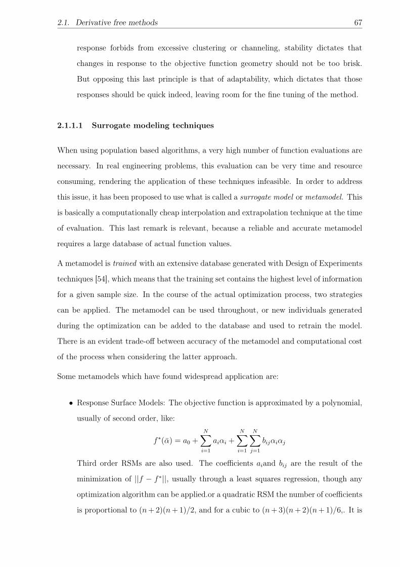
2.1. Derivative free methods 67
response forbids from excessive clustering or channeling, stability dictates that
changes in response to the objective function geometry should not be too brisk.
But opposing this last principle is that of adaptability, which dictates that those
responses should be quick indeed, leaving room for the fine tuning of the method.
2.1.1.1 Surrogate modeling techniques
When using population based algorithms, a very high number of function evaluations are
necessary. In real engineering problems, this evaluation can be very time and resource
consuming, rendering the application of these techniques infeasible. In order to address
this issue, it has been proposed to use what is called a surrogate model or metamodel. This
is basically a computationally cheap interpolation and extrapolation technique at the time
of evaluation. This last remark is relevant, because a reliable and accurate metamodel
requires a large database of actual function values.
A metamodel is trained with an extensive database generated with Design of Experiments
techniques [54], which means that the training set contains the highest level of information
for a given sample size. In the course of the actual optimization process, two strategies
can be applied. The metamodel can be used throughout, or new individuals generated
during the optimization can be added to the database and used to retrain the model.
There is an evident trade-off between accuracy of the metamodel and computational cost
of the process when considering the latter approach.
Some metamodels which have found widespread application are:
• Response Surface Models: The objective function is approximated by a polynomial,
usually of second order, like:
f ∗(α) = a0 +N∑i=1
aiαi +N∑i=1
N∑j=1
bijαiαj
Third order RSMs are also used. The coefficients aiand bij are the result of the
minimization of ||f − f ∗||, usually through a least squares regression, though any
optimization algorithm can be applied.or a quadratic RSM the number of coefficients
is proportional to (n+ 2)(n+ 1)/2, and for a cubic to (n+ 3)(n+ 2)(n+ 1)/6,. It is
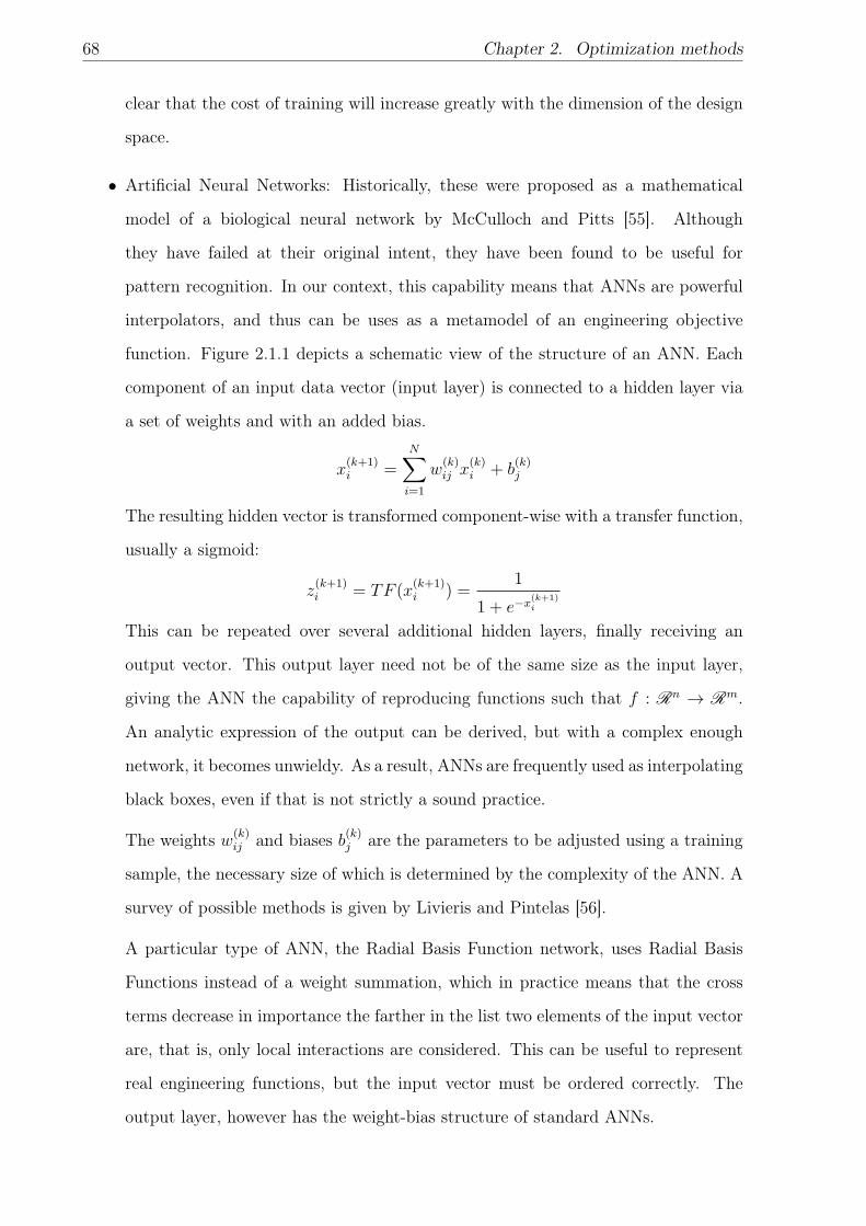
68 Chapter 2. Optimization methods
clear that the cost of training will increase greatly with the dimension of the design
space.
• Artificial Neural Networks: Historically, these were proposed as a mathematical
model of a biological neural network by McCulloch and Pitts [55]. Although
they have failed at their original intent, they have been found to be useful for
pattern recognition. In our context, this capability means that ANNs are powerful
interpolators, and thus can be uses as a metamodel of an engineering objective
function. Figure 2.1.1 depicts a schematic view of the structure of an ANN. Each
component of an input data vector (input layer) is connected to a hidden layer via
a set of weights and with an added bias.
x(k+1)i =
N∑i=1
w(k)ij x
(k)i + b
(k)j
The resulting hidden vector is transformed component-wise with a transfer function,
usually a sigmoid:
z(k+1)i = TF (x
(k+1)i ) =
1
1 + e−x(k+1)i
This can be repeated over several additional hidden layers, finally receiving an
output vector. This output layer need not be of the same size as the input layer,
giving the ANN the capability of reproducing functions such that f : Rn → Rm.
An analytic expression of the output can be derived, but with a complex enough
network, it becomes unwieldy. As a result, ANNs are frequently used as interpolating
black boxes, even if that is not strictly a sound practice.
The weights w(k)ij and biases b(k)
j are the parameters to be adjusted using a training
sample, the necessary size of which is determined by the complexity of the ANN. A
survey of possible methods is given by Livieris and Pintelas [56].
A particular type of ANN, the Radial Basis Function network, uses Radial Basis
Functions instead of a weight summation, which in practice means that the cross
terms decrease in importance the farther in the list two elements of the input vector
are, that is, only local interactions are considered. This can be useful to represent
real engineering functions, but the input vector must be ordered correctly. The
output layer, however has the weight-bias structure of standard ANNs.
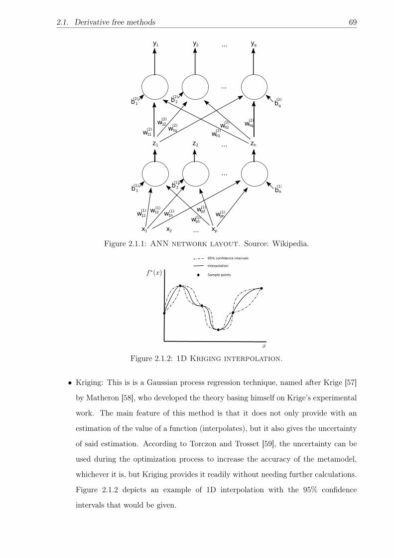
2.1. Derivative free methods 69
x1 x2 xp...
z1 z2 zh...
...
w11w12 w1h wph
b1 bh
(1) b2(1)
(1)
(1)(1)
(1)
wp1(1)
wp2(1)
(1)
y1 y2 yq...
...
b1 b(2) b2
(2)(2)
q
w11(2)
w12(2)
w1q(2)
wh1(2)wh2(2) whq
(2)
Figure 2.1.1: ANN network layout. Source: Wikipedia.
Sample points
Interpolation
95% confidence intervals
Figure 2.1.2: 1D Kriging interpolation.
• Kriging: This is is a Gaussian process regression technique, named after Krige [57]
by Matheron [58], who developed the theory basing himself on Krige’s experimental
work. The main feature of this method is that it does not only provide with an
estimation of the value of a function (interpolates), but it also gives the uncertainty
of said estimation. According to Torczon and Trosset [59], the uncertainty can be
used during the optimization process to increase the accuracy of the metamodel,
whichever it is, but Kriging provides it readily without needing further calculations.
Figure 2.1.2 depicts an example of 1D interpolation with the 95% confidence
intervals that would be given.
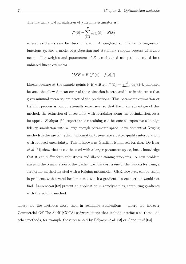
70 Chapter 2. Optimization methods
The mathematical formulation of a Kriging estimator is:
f ∗(x) =K∑j=1
βjgj(x) + Z(x)
where two terms can be discriminated. A weighted summation of regression
functions gj, and a model of a Gaussian and stationary random process with zero
mean. The weights and parameters of Z are obtained using the so called best
unbiased linear estimator.
MSE = E[(f ∗(x)− f(x))2]
Linear because at the sample points it is written f ∗(x) =∑N
i=1 wif(xi), unbiased
because the allowed mean error of the estimation is zero, and best in the sense that
gives minimal mean square error of the predictions. This parameter estimation or
training process is computationally expensive, so that the main advantage of this
method, the reduction of uncertainty with retraining along the optimization, loses
its appeal. Shahpar [60] reports that retraining can become as expensive as a high
fidelity simulation with a large enough parameter space. development of Kriging
methods is the use of gradient information to generate a better quality interpolation,
with reduced uncertainty. This is known as Gradient-Enhanced Kriging. De Baar
et al [61] show that it can be used with a larger parameter space, but acknowledge
that it can suffer form robustness and ill-conditioning problems. A new problem
arises in the computation of the gradient, whose cost is one of the reasons for using a
zero order method assisted with a Kriging metamodel. GEK, however, can be useful
in problems with several local minima, which a gradient descent method would not
find. Laurenceau [62] present an application in aerodynamics, computing gradients
with the adjoint method.
These are the methods most used in academic applications. There are however
Commercial Off-The Shelf (COTS) software suites that include interfaces to these and
other methods, for example those presented by Belyaev et al [63] or Gano et al [64].
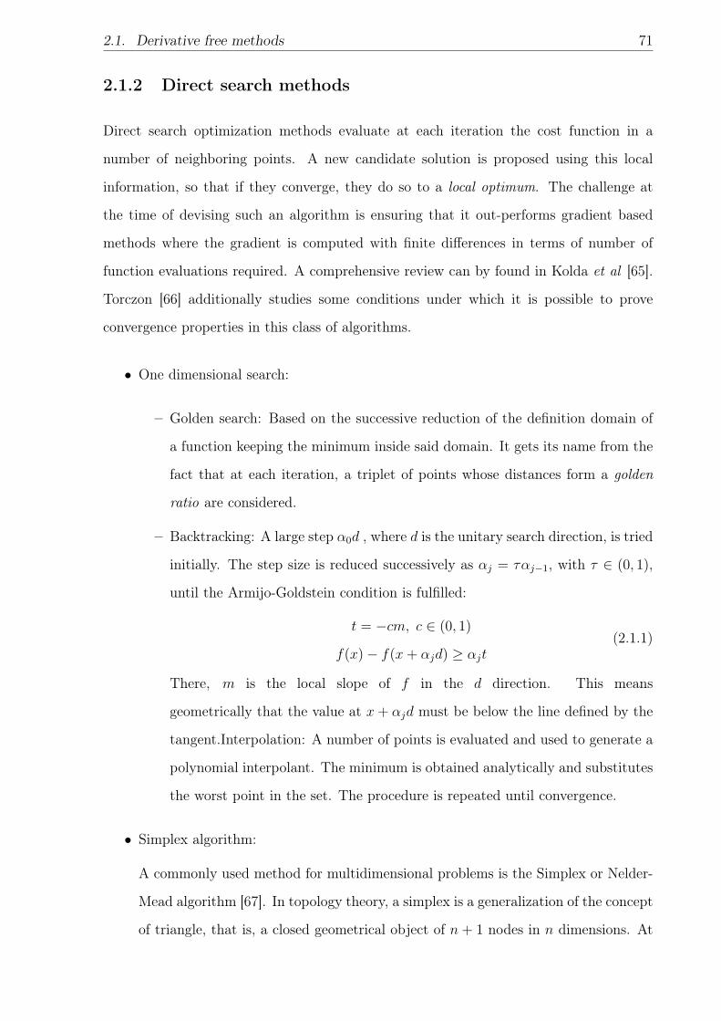
2.1. Derivative free methods 71
2.1.2 Direct search methods
Direct search optimization methods evaluate at each iteration the cost function in a
number of neighboring points. A new candidate solution is proposed using this local
information, so that if they converge, they do so to a local optimum. The challenge at
the time of devising such an algorithm is ensuring that it out-performs gradient based
methods where the gradient is computed with finite differences in terms of number of
function evaluations required. A comprehensive review can by found in Kolda et al [65].
Torczon [66] additionally studies some conditions under which it is possible to prove
convergence properties in this class of algorithms.
• One dimensional search:
– Golden search: Based on the successive reduction of the definition domain of
a function keeping the minimum inside said domain. It gets its name from the
fact that at each iteration, a triplet of points whose distances form a golden
ratio are considered.
– Backtracking: A large step α0d , where d is the unitary search direction, is tried
initially. The step size is reduced successively as αj = ταj−1, with τ ∈ (0, 1),
until the Armijo-Goldstein condition is fulfilled:
t = −cm, c ∈ (0, 1)
f(x)− f(x+ αjd) ≥ αjt(2.1.1)
There, m is the local slope of f in the d direction. This means
geometrically that the value at x+ αjd must be below the line defined by the
tangent.Interpolation: A number of points is evaluated and used to generate a
polynomial interpolant. The minimum is obtained analytically and substitutes
the worst point in the set. The procedure is repeated until convergence.
• Simplex algorithm:
A commonly used method for multidimensional problems is the Simplex or Nelder-
Mead algorithm [67]. In topology theory, a simplex is a generalization of the concept
of triangle, that is, a closed geometrical object of n + 1 nodes in n dimensions. At
72 Chapter 2. Optimization methods
Best
Other
Worst
ReflectedCentroid
Best
Other
Worst
Worst'
Other'
Figure 2.1.3: Left, Simplex method candidate point generation. Right,Shrinking when candidates are not accepted.
each iteration the simplex is modified discarding the worst performing node and
creating an improved one, using geometric operations.
First, a centroid is computed as the average of the simplexes points. Next, an
imaginary line is created, that goes though the centroid and is normal to the segment
that joins the best and other points. The new candidates are the centroid itself
and its reflection in that line. In each iteration of simplex optimization, if one
of the candidates is better than the current worst solution, worst is replaced by
that candidate. But if none of the candidates generated is better than the worst
solution, the current worst and other solutions shrink toward the best solution to
points somewhere between their current position and the best solution. Figure 2.1.3
illustrates these two possibilities.
After each iteration, a new virtual best-other-worst triangle is formed, getting closer
and closer to an optimal solution. If you imagine taking a snapshot of each triangle
over time, when looked at sequentially, the triangles move in a way that resembles an
amoeba. For this reason, simplex optimization is sometimes called amoeba method.
Variations on the algorithm considering different points along the centroid reflection
line, or translations of the whole simplex, can be formulated.
One could question the review on one dimensional methods, as real engineering problems
are multidimensional. In practice, these are not used for the search itself, but as an
intermediate auxiliary step that improves convergence of a calling method that has already
defined a search direction. For example, they can be used to search for the best candidate
2.2. Local derivative based methods 73
solution in the reflection line in a Simplex algorithm, as Custódio and Vicente [68] do.
But their most common use is found in conjunction with multidimensional gradient based
methods for constrained problems, which will be spoken of in section .
2.2 Local derivative based methods
These methods use sensitivity information to construct a search direction. Simple
algorithms, such as Steepest Descent,may use it directly, but this is an inefficient approach.
Effective algorithms use more complex strategies [69].
• Newton method:
This method solves the nonlinear equation that nullifies the gradient. The Newton
method for nonlinear root finding uses first order sensitivity directly to build a search
direction, which in the case of optimization translates into the need of computing the
Hessian, or second order sensitivity. This method is seldom used due to numerical
problems and the frequently infeasible complexity of generating the Hessian.
• Quasi Newton methods:
If the minimization problem has a solution, it is safe to assume that the Hessian
is positive definite. And if small perturbations in design parameters are assumed
as linearly interacting, it is also symmetric. There are methods that can generate
positive definite symmetric matrices out of algebraic operations on vectors, and are
used to approximate the Hessian using gradient information, thus giving rise to a
class of Quasi-Newton methods.
• Conjugate gradient methods:
These represent the application of Krylov subspace iterative methods to solving the
null gradient equation.
• Sequential programming:
Newton and Quasi-Newton methods suffer from a small convergence radius, and
the standard Newton’s method may become unstable if the Hessian is not positive
74 Chapter 2. Optimization methods
definite. To overcome these issues, smaller sub-problems can be solved in nested
iterations, before exploring further in outer iterations.
If what is reduced is the dimension of the problem, it is spoken of line-search
methods. These define a search direction and find the distance which minimizes
the objective function in it, solving a one dimensional sub-problem. When this
provisional optimum is found, a new search direction is defined in an outer iteration.
When using gradients, the Armijo-Goldstein condition presented in equation 2.1.1
for backtracking line search can be completed with equation 2.2.1, where 0 < c <
c2 < 1. This conditions means that the slope is forced to increase at each step.
Bearing in mind that in a minimization problem the slope is negative, the aim is to
increase it until it reaches zero. Then it is spoken of the Wolfe conditions.
dT · ∇f(x+ αjd) ≥ c2dT · ∇f(x) (2.2.1)
If what is limited is the step size, it is spoken of trust region methods. The maximum
step size defines a small subdomain in which the minimum is found, after which the
outer iteration relocates the design to a nearby more promising sub-domain.
To solve the inner and outer problems, any of the previously described methods can
be used. In the case of trust region methods, however, it is often the case that a
certain behavior of objectives and constraints is assumed, speaking then of linear
programming or quadratic programming.
2.3 Constraint treatment
All the described algorithms are meant to solve an unconstrained optimization problem.
In this section, it is described how constraints can be made to fit into that framework.
This is a most important topic, as in reality, engineering problems are more a question
of finding a solution that meets the requirements (constraints), than actually minimizing
some metric.
2.3. Constraint treatment 75
2.3.1 Lagrange multipliers
Recall the definition of the optimization problem, where the design space is restricted due
to the equality constraints hk and inequality constraints gj. Assuming a single objective
function, the so called Lagrangian function can be built by adding the contribution of the
active set of constraints to it, such as:
I(x) = f(x) +
Q∑k=0
λkhk(x) +P−I∑j=0
µjgj(x) (2.3.1)
The active set of constraints is formed by hk and those gj such that gj > 0, that
is, the unfulfilled inequality constraints. We define I as the number of inactive, or
fulfilled, inequality constraints. Bound constraints can be reformulated as inequality
constraints.Lagrange multipliers are used in conjunction with gradient based methods, and
the minimization problem becomes the solution to the problem of fulfilling the Karush-
Kuhn-Tucker conditions:
dfdx
+∑Q
k=0 λkdhkdx
+∑P−I
j=0 µjdgjdx
= 0
gj(α) = 0 j = 1, P − I
hk(α) = 0 k = 1, Q
(2.3.2)
A gradient based algorithm will provide a search direction which may result in inactive
constraints becoming active, or straying too far from the equality restrictions. This is
prevented using line search methods and monitoring the Lagrangian (not merely the
objective function) or using penalty functions. Gilbert [70] reports a penalty function
approach devised by Pschenichny, whose original reference is hard to find.
Lagrange multipliers can be interpreted geometrically, or in the light of game theory.
Rockafellar [71] gives thorough account of both interpretations. When using game theory,
the concept of duality arises. Naming x the primal variable, and λ the dual variable, it can
be shown that the KKT conditions are equivalent to the so called saddle point condition,
where two problems are simultaneously solved, that of the minimization of the Lagrangian
with respect to the primal, and its maximization with respect to the dual variable. This
combined problem can be modeled as a two person zero-sum game, and the saddle point
is an equilibrium state. This interpretation opens the door to algorithms that solve the
dual problem instead, in cases where this may be simpler.
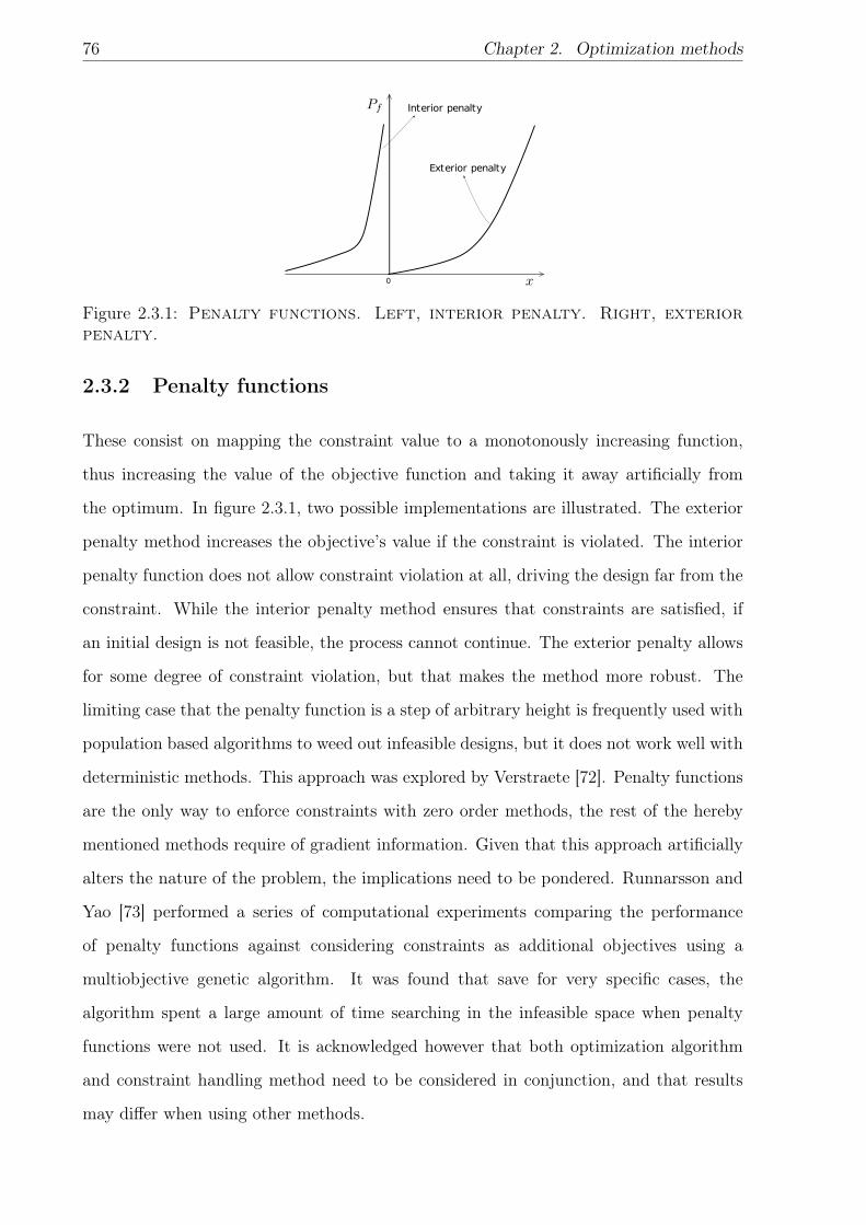
76 Chapter 2. Optimization methods
Interior penalty
Exterior penalty
0
Figure 2.3.1: Penalty functions. Left, interior penalty. Right, exteriorpenalty.
2.3.2 Penalty functions
These consist on mapping the constraint value to a monotonously increasing function,
thus increasing the value of the objective function and taking it away artificially from
the optimum. In figure 2.3.1, two possible implementations are illustrated. The exterior
penalty method increases the objective’s value if the constraint is violated. The interior
penalty function does not allow constraint violation at all, driving the design far from the
constraint. While the interior penalty method ensures that constraints are satisfied, if
an initial design is not feasible, the process cannot continue. The exterior penalty allows
for some degree of constraint violation, but that makes the method more robust. The
limiting case that the penalty function is a step of arbitrary height is frequently used with
population based algorithms to weed out infeasible designs, but it does not work well with
deterministic methods. This approach was explored by Verstraete [72]. Penalty functions
are the only way to enforce constraints with zero order methods, the rest of the hereby
mentioned methods require of gradient information. Given that this approach artificially
alters the nature of the problem, the implications need to be pondered. Runnarsson and
Yao [73] performed a series of computational experiments comparing the performance
of penalty functions against considering constraints as additional objectives using a
multiobjective genetic algorithm. It was found that save for very specific cases, the
algorithm spent a large amount of time searching in the infeasible space when penalty
functions were not used. It is acknowledged however that both optimization algorithm
and constraint handling method need to be considered in conjunction, and that results
may differ when using other methods.

2.3. Constraint treatment 77
2.3.2.1 Augmented Lagrangian
The Augmented Lagrangian method is the application of a penalty function with an
adaptive weight such that it approximates the true Lagrange multiplier. The method is
explained using a single equality constraint for simplicity. Adding a quadratic term to
the Lagrangian, such as:
AI(x) = f(x) + λh(x) +1
2µh(x) · h(x) (2.3.3)
The minimization of the Lagrangian implies finding the zero of the differential:
dAI
dx=df
dx+ (λ+
h
µ)dh
dx= 0 (2.3.4)
At a solution of the problem, it is the case that:
df
dx+ λ∗
dh
dx= 0 (2.3.5)
Thus an iterative updating method for λ can be deduced as:
λ(k+1) = λ(k) +h(x(k+1))
µ(2.3.6)
The additional parameter µ is a mathematical device intended to provide a way of
approaching an asymptotically exact solution. Given that h → 0 as we approach the
solution, the update of the multiplier would become slower. Driving µ towards zero as
the process progresses prevents its stagnation.
2.3.2.2 Interior point methods
The interior point method is a refinement of the application of an interior penalty function
borrowing the Lagrange multiplier estimation concept from the Augmented Lagrangian
approach. Consider a problem with only inequality constraints, like:
Minimize fi(α) i = 1, N (2.3.7)
Subject to gj(α) > 0 j = 1, P
The constraints are added to the objective function with a penalty function that is not
defined below zero, and tends to infinity in its vicinity. Such a function can be the
78 Chapter 2. Optimization methods
logarithm. The full barrier function is given like:
B(x) = f(x)− µP∑j=0
log[gj(x)] (2.3.8)
and the stationary point is found with:
dB
dx=df
dx−
P∑j=0
µ
gj
dgjdx
= 0 (2.3.9)
If gj were equality constraints, the associated Lagrange multiplier would be computed as
λj = µ/gj. The optimization problem can be rewritten as:
df
dx+∑P
j=0 λjdgjdx
= 0
λjgj(α) = µ j = 1, P(2.3.10)
Wächter [74] has developed an open source optimization library, IpOpt, based on the
interior point approach, using a Quasi-Newton or Newton (if the user is able to produce
the Hessian matrices of objectives and constraints) search to solve the stationary point
equation, which has been tested in the course of this work with good results in certain
problems.
2.3.2.3 Kreisselmeier-Steinhauser method.
The Kreisselmeier-Steinhauser method is another penalty function based method for
constraint aggregation. Chattopadhyay and Rajadas [75] describe the original method
as well as an improvement on it adding user defined weighting factors intended to assign
preference (see section 2.4.2). Using this approach, the objective functions to be minimized
are reformulated as constraints, like:
fi(α) =fi(α)
fi,0− 1− gmx ≤ 0
where gmx is the largest constraint value. Given that equality constraints can be
trivially reformulated as two inequality constraints, a new constraint vector φ of size
M = N + P + 2Q can be built considering the reformulated objectives in conjunction
with the original constraints. This constraint vector is scalarized like
FKS(α) = φmx −1
ρ
M∑m=1
eρ·[φ(α)−φmx] ≤ 0
2.4. Selecting a single solution 79
where φmx is the largest constraint in the the new constraint vector (not necessarily the
same as gmx ).Using this formulation, when the original constraints are satisfied during
the process, the constraints due to the reformulated objectives are violated, and thus the
optimizer will minimize the objectives. If searching an infeasible region of the design
space, the opposite situation is true, and the optimizer will try to find a feasible region,
ignoring momentarily the minimization of objectives. The parameter ρ has the effect of
making the aggregated function more similar to the currently most violated constraint
for large values. For low values, contributions from all constraints are considered at all
times. One of the previously mentioned authors has used the method for an application
in the multidisciplinary design of propfan blades, see Chattopadhyay and McCarthy [76].
2.4 Selecting a single solution
2.4.1 Normalization
In all these considerations, no mention has been given to the fact that different objectives
are mathematical formulations of different physical phenomena, measured in different
units, and taking values of potentially vastly different orders of magnitude. Articulating
a preference can only be done between commensurable magnitudes, that is, measured in
the same units and varying in the same interval, and thus, objectives and constraints need
to be normalized.
Several normalization approaches can be taken:
• Divide by the value at the initial point: fi(x) = fi(x)/fi(x0).
• Divide by the maximum of the objective functions: fi(x) = fi(x)/fi(x∗), where x∗is
the solution to min fi(x) .
• Normalize using the Nadir and Utopia points: fi(x) = (fi(x)−fUi )/(fNi −fUi ). The
Nadir points, fNi , and the Utopia points, fUi , bound the Pareto front. Effectively, the
Utopia points will be the solution to the isolated minimization of each objective, and
the Nadir is the maximum value that a single objective can take when minimizing
80 Chapter 2. Optimization methods
the rest. In practice, computation of the Nadir and Utopia points is not feasible in
general, but there are cases when engineering judgment can approximate them.
The first two schemes have been shown to be ineffective [77], but at least the first one
is easy to compute. Thus it is frequently used, even if it does not give the best results.
Even more, if the initial value is zero, it directly cannot be used. The third schema is
the most theoretically sound, giving proper scaling of the optimal set, so that assigning
weights has proper meaning. However, its application is not practical in most cases.
2.4.2 Preference articulation methods
For a multiobjective optimization problem, a Pareto optimal set of solutions will exist.
The question of which individual to choose can be answered by specifying an articulation
of preferences. This preference articulation can be used before starting the optimization
process (a priori), so that it includes the information of the different objectives into a
single scalar. Then it can be spoken of scalarization techniques. This approach gives
a single solution as a result, and is preferred when placing emphasis on speed. Another
approach is to generate a dense Pareto set, and select a posteriori the appropriate solution.
This method would be preferred when time is not a constraint, and the designer wishes
to explore the design space in detail.
A comprehensive survey of both a priori and a posteriori methods is given by Marler and
Arora [78], in addition to techniques used by population based algorithms. In this thesis,
the multiobjective optimization problem is solved with a single objective algorithm, so a
scalarization technique must be used. Below, a number of these preference articulation
methods are briefly described, including the techniques that have been finally chosen.
• A priori methods: These are based mainly in some kind of weighted aggregation.
The immediate pitfall is that without proper normalization, a set of weights may
not be an accurate representation of the preferences.
– Weighted exponential sum: This method can be interpreted as the minimiza-
tion of a p−norm. For p = 1 it reduces to a simple weighted sum. For p→∞,
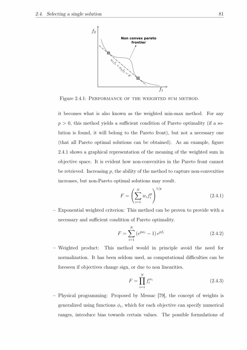
2.4. Selecting a single solution 81
Non convex pareto frontier
Figure 2.4.1: Performance of the weighted sum method.
it becomes what is also known as the weighted min-max method. For any
p > 0, this method yields a sufficient condition of Pareto optimality (if a so-
lution is found, it will belong to the Pareto front), but not a necessary one
(that all Pareto optimal solutions can be obtained). As an example, figure
2.4.1 shows a graphical representation of the meaning of the weighted sum in
objective space. It is evident how non-convexities in the Pareto front cannot
be retrieved. Increasing p, the ability of the method to capture non-convexities
increases, but non-Pareto optimal solutions may result.
F =
(N∑i=1
wifpi
)1/p
(2.4.1)
– Exponential weighted criterion: This method can be proven to provide with a
necessary and sufficient condition of Pareto optimality.
F =N∑i=1
(epwi − 1) epfi (2.4.2)
– Weighted product: This method would in principle avoid the need for
normalization. It has been seldom used, as computational difficulties can be
foreseen if objectives change sign, or due to non linearities.
F =N∏i=1
fwii (2.4.3)
– Physical programming: Proposed by Messac [79], the concept of weights is
generalized using functions φi, which for each objective can specify numerical
ranges, introduce bias towards certain values. The possible formulations of
82 Chapter 2. Optimization methods
these preference functions given by Messac resemble penalty functions, which
exemplifies how a given problem can be formulated in several ways.
F = log
[1
N
N∑i=1
φi(fi)
](2.4.4)
– Hierarchical, lexicographic and ε−constraint methods: These methods are
different implementations of the concept of ordering the objectives in terms
of importance assigned by a decision maker, and solving sequentially a single
objective problem. Constraints are successively added on the increase of
previously minimized objectives. Chircop and Zammit-Mangion [80] propose
an implementation that is claimed to be robust even for ill conditioned
problems.
• A posteriori methods: An advantage when using these is that the Nadir and Utopia
points are already computed, so that a proper normalization can be applied.
– Normal Boundary Intersection: This methods extracts an even distribution
of Pareto optimal points for consistent weight variations for both convex and
non-convex Pareto frontiers. The first step is to find the boundaries of the
Pareto set, computing the Utopia points. The normal hyperplane is the one
that passes through the Utopia points. The idea of the method is to find the
nearest point of the Pareto set to the normal hyperplane in its characteristic
direction. For a bi-objective problem, it is formulated as follows. Given an
arbitrarily populated Pareto set, the minimization problem is posed,
Minimize λ (2.4.5)
Subject to(fi(x
∗i )− fUi
)· (w − λe) = fi(x)− fUi i = 1, N
where e is a vector of ones in objective space, w is a vector of weights to be
systematically varied to define the mesh, and f(x∗i ) is the vector of objective
functions evaluated at the minimum of the ith objective.
– Normal Constraint method: A development of the previous method, the normal
hyperplane is parametrized and meshed, and the solutions extracted are the
projections of the Pareto set in the normal hyperplane mesh.
2.5. Sensitivity computation techniques 83
2.5 Sensitivity computation techniques
Gradient information is either necessary or useful in several optimization algorithms, so
an important aspect of solving the problem is its accurate and practical computation.
2.5.1 Finite differences
Arbitrary order derivatives can be computed within a required precision [81] with different
formulas. In essence, computing a number of objective function values for perturbations
around a given design allows to estimate the derivative. This approach ceases to have
practical use when the objective function is expensive to evaluate.
2.5.2 Complex step differentiation
Numerical differentiation formulas are subject to round-off errors when using very small
step sizes. Knowing which is an appropriate perturbation size for a given function is
in itself a difficult sensitivity analysis problem, as minimizing round-off and truncation
error are conflicting requirements. An approach that works around this problem is that
of complex step numerical differentiation. Perturbing the independent variables in well
chosen directions in the complex plane, the issue of subtractive cancellation is avoided.
For first and second order derivatives, the complex step expressions are given by:
df
dx=Im[f(x0 + ih)]
hd2f
dx2=Im[f(x0 +
√2
2(1 + i)h)] + Im[f(x0 −
√2
2(1 + i)h)]
h2
as derived by Lai et al [82]. Arbitrary order derivatives can be computed using multi-
complex algebra, as shown by Lantoine et al [83].
2.5.3 Algorithmic differentiation
Frequently referred to as automatic differentiation, although, as reminded by Griewank
and Walther [84], it is seldom an automatic process. Given a computer program that
gives some numerical output, a technology can be devised to parse the code and apply the
84 Chapter 2. Optimization methods
chain rule successively to simple operations (sum, multiplication, division, trigonometric
functions, etc.) in order to generate some code that evaluates the derivative of the original
one.
State of the art technology [85] is capable providing with high order derivatives in theory.
In practice, complex programming techniques such as parallelization and heterogeneous
language usage, prevent from building a truly automatic procedure.
Algorithmic differentiation can be performed in two ways. Forward sensitivity
propagation, also known as tangent derivatives, provide the sensitivity of the output
to input perturbations. Reverse sensitivity propagation, or adjoint sensitivities, do so for
the inputs with respect to output variations. These two modes can be represented as:
Forward mode: y = F ′x
Reverse mode: xT = yTF ′(2.5.1)
The latter mode of differentiation is named reverse mode because it is directly linked
to the concept of adjoint operator in operator theory. More is said about this topic in
the following section. If the application of algorithmic differentiation is possible for the
problem at hand, it provides with derivatives with no round-off error issues.
2.5.4 Adjoint method
In some cases the objective function can be expressed as a functional of a field operator
I acting over the design vector, subject to some state equations F . Defining y = dy/dα,
the gradient of I with respect to the design vector can be written as:
I = I(α, y)⇒ dIdα
= ∂I∂α
+ ∂I∂yy (2.5.2)
Additionally, for any design vector, the state equations are fulfilled, which means that the
variation in the residual of state equations is zero.
F (α, y) = 0⇒ L y|Ω + By|∂Ω = −∂F∂α
(2.5.3)
There, L is the jacobian of the state equations, and B is a suitable boundary
conditions operator.The sensitivity could be evaluated by finite differences or tangent
mode algorithmic differentiation applying the necessary perturbations y. It is evident
2.5. Sensitivity computation techniques 85
that the cost of this operation grows at least linearly with the design space size. To
circumvent this problem, it is possible to use adjoint operator theory [86], to translate
the direct problem of equating the gradient in 2.5.2 to zero subject to 2.5.3 into the dual
problem
I = I(α, y)⇒ dIdα
= ∂I∂α− v ∂F
∂α(2.5.4)
subject to
F (α, y) = 0⇒ L ∗v|Ω + B∗v|∂Ω = −∂F∂α
(2.5.5)
where the subscript ∗ denotes the Hermitian conjugate.
The decision to work with continuous or discrete operators has its implications.
Ultimately, the field state equations will be evaluated numerically in a discrete mesh
with a certain computer code. A code that represents its adjoint operator will then be
also discrete. But this adjoint operator can have been derived from the continuous primal
operator of from the discretized one. Nadarajah and Jameson [87] study the differences
in performance and cost of development of each approach for the RANS equations. They
found that the discrete approach results in more accurate gradients, as the adjoint is
built on the actual solved equations. The continuous approach results in an easier and
more flexible development, as the equations can be discretized in a different way than
the primal, if judged to be convenient. It has to be reminded that discrete operators
for physics simulations can be very complex, and thus, difficult to derive an adjoint
version. But the continuous formulation has some pitfalls. Arian and Salas [88] show that
the continuous formulation cannot admit directly certain objective functions. For these
incomplete functionals, additional terms must be derived to close the adjoint problem,
which in general is not straightforward. Also, the boundary product is a difficult term to
work with. Working with matrices (discrete operators), it disappears.
As a last remark, recalling equation 2.5.1, making xT = (∂I/∂y)T , reveals that it
is possible to implement a procedure to solve for the adjoint variable y by reverse
differentiating a code that gives F (α, y). Several authors [89, 90, 91, 92, 93] have
worked in this direction, revealing the practical difficulties as well as the real advantages
offered by this approach when applied to CFD. Some authors [94, 95, 96] use automatic
differentiation to compute not only first order derivatives, but second order, and use them
86 Chapter 2. Optimization methods
in optimization applications using Newton methods.
2.5.4.1 One-shot optimization
Due to the efficiency in sensitivity computation in Partial Differential Equation
constrained problems afforded by the adjoint method, it is used within the framework
of what are called One-shot methods. In a conventional approach, for each design
iteration, a PDE solver is run in order to postprocess a converged state and compute
the objective metrics. Sensitivities would be then computed using the adjoint solution.
This information is fed to the optimizer so that it can propose a design vector update. In
a One-shot approach, the design variables, PDE state variables, and adjoint variables are
iterated simultaneously, using the same solver. Griewank [97] explains the method, and
how Hessians computed with automatic differentiation can be used to make the procedure
more efficient. Günther et al [98] develop an extension of the method to be used with
unsteady PDEs.
One hurdle to the application of this approach is the fact that some design variables may
affect the state vector only locally. Hazra [99] proposes to use multigrid techniques, where
design parameters affecting the state vector globally are modified in coarser grids, and
parameters with local influence are modified in finer meshes.
But the main disadvantage of the method is the radically different nature of the
optimization problem with respect to the PDE solution. Algorithms suited for one
problem will not necessarily perform well in the other context, and constraints not
depending on the state vector become very difficult to treat.
Chapter 3
Automatic design environment
Product design in industry is an iterative process, where several experts in different
engineering disciplines give their input in a cyclical manner. Given that much of the work
is repetitive in nature, it is conceivable to automatize the process. A possible hazard is the
waste of accrued human experience and knowledge, an effort must be made to integrate
it within any automatic procedure. Shahpar [100] notes a number of requirements that
an Automatic Design Optimization (ADO) system must fulfill for it to be actually useful,
while acknowledging that several hurdles are in place for the routine adoption of these
techniques, not all of them being of technical nature.
In this context of turbomachinery component design, the problem can be described
as the definition of a geometrical shape such that, when physically realized through a
specific manufacturing process, achieves some functional requisites and performance goals
subject to certain constraints. The whole problem is multidisciplinary in nature, requiring
the information provided by conceptual design tools, detailed numerical analyses, and
manufacturing process experts. In the normal practice of industrial human driven design,
adepts of each discipline are organized into different teams, with different levels of
interaction during the design iterations according to established best practices within
the company. An ADO system can be implemented to encompass as much of this process
as possible, or to be restricted to one aspect. This will impose requirements in terms of
optimization algorithms, interfaces with external geometry generation and multi-physics
analysis tools, and how additional knowledge is applied.
87
88 Chapter 3. Automatic design environment
Regarding the choice of optimization algorithm, there are different classes according
to their local or global convergence properties, their handling of constraints, or their
need of gradient information. The application developed by Rolls Royce, SOPHY [101],
intended to be used for different classes of problems, has a wide array of methods available,
acknowledging the fact that no single algorithm is clearly superior to the rest for a wide
range of applications. CADO, developed by Verstraete [102], and AutoOpti, developed at
the DLR [103], use population based evolutionary optimization algorithms, assisted with
metamodelling techniques. They have been applied for the design of both axial and radial
turbomachinery components.
When the optimization algorithm to be used requires the use of first order derivatives,
there is the added level of complexity of computing these. Finite difference methods,
whether using real or complex step formulations [82], are infeasible when dealing with
industrial size problems. Thus, the use of adjoint methods, which provide gradient
information independently of the size of the design space, is advocated in these cases.
These methods were pioneered by Glowinski and Pironneau [104] and introduced to the
aerospace community by Jameson [105]. Since then, a number of works have popularized
the method throughout industry and academia (see Giles [86]), moving beyond single
operation point aerodynamic design problems. For instance, full aero-structural coupling
with the use of adjoint methods is reported by Martins et al [106] for aircraft design.
The turbomachinery community was slower in experimenting with adjoint methods. Duta
et al [107], present a pioneering study in this context, introducing at the same time a
frequency domain unsteady adjoint method. Independently of the optimization algorithm,
examples of aerodynamic design applications exist in literature belonging mainly to two
distinct classes. The first one comprises works where 3D optimization is performed
monitoring objective functions evaluated at the outlet section in internal flows, such as
losses, massflow matching, etc. whether in single row (see an application to compressor
aerodynamic design by Benini [108]) or multiple row applications (see Okui et al [109],
Wang and He [110] or Walther and Nadarajah [111]). To the other class belong works
demonstrating how the inverse design problem can be solved using CFD and optimization
techniques. Most published works describe just 2D aerodynamic design problems, for
example Li et al [112]. Applications to the full three dimensional problem, while more
89
scarce, do exist (see Wang and Li [113] and van Rooij et al [114]).
These two classes of problems are not mutually exclusive. In fact, in the current state of
CFD, turbulence and transition cannot be resolved. Various modelling approaches incur
into different degrees of error (see Wilcox [20]), and given the influence of these phenomena
in loss generation (as reported by Mayle [115] and Walker [116]), it is concluded that
profile losses computed making solely use of CFD cannot be accurate. It also has to
be remembered that a design project operates within tight time frames, so that solution
accuracy has to be balanced with design lead time to meet deadlines. In normal practice,
instead of minimizing losses, designers generate a loading shape that is known to be
well performing from previous experimental or very high fidelity CFD modelling studies.
In addition, the full 3D airfoil has to fulfill mass-flow and outlet angle requirements,
and has as little work loss due to secondary flows as possible. Thus, a well posed
aerodynamic design problem is a combination of the previously mentioned problem classes.
Finally, further issues unrelated to aerodynamics will need to be ultimately translated into
geometrical constraints.
Drela [117] performed a computational experiment to illustrate the importance of the
definition of the optimization problem, in terms of selection of both design space and
objective functions. In a 2D profile optimization exercise, stemming from a known airfoil
shape, he applied sinusoidal shape perturbations with the aim of minimizing drag. Lift
was to remain constant through an appropriate constraint. Constraints on thickness and
other area properties were imposed after initial failed experiments where the optimizer
gravitated towards non-manufacturable geometries. It was found that the optimizer
tended to make use of the smallest geometrical scales. This meant that an improved airfoil
was found for the specific operating point of the optimization, while the performance
envelope was degraded elsewhere. These results highlight the need to analyze several
operating points, which is known as multipoint optimization, which, in turn, is one of the
various techniques of robust optimization. A robust design is that whose performance is
affected less from parameter variations. Sources of variability in an engineering design
problem can be classified into two groups, according to Chen et al [118]:
• Uncertainties in the design parameter space: Also called uncertainties in control
90 Chapter 3. Automatic design environment
factors. In a shape optimization problem, these are translated into geometrical
variations due to manufacturing tolerances.
• Uncertainties in noise factors: Also called uncertainties in uncontrollable parame-
ters. In an aerodynamic design problem, they can imply variability in the boundary
conditions for a certain design point. Uncertainties due to errors in CFD modeling,
not guaranteeing mesh independent results, etc... also belong here.
Robust design problems can be posed for both classes of uncertainties, for which both
deterministic and probabilistic methods have been devised. An account is given by Beyer
and Sendhoff [119]. It is worth noting that there are deterministic methods that use
first order sensitivity information, the basic idea being to limit the slope of the objective
function around the robust solution. Other methods use up to second order sensitivity, the
robust solution being the one with reduced curvature. The most common of probabilistic
methods is the Monte Carlo approach [120], for which a candidate solution is evaluated
for a range of the uncertain parameters in order to compute the relevant statistics, and
the robust design will be the one with reduced variance. The problem with this approach
is the large number of evaluations to perform, as statistics converge slowly. For instance,
the convergence rate of the mean is ∝ 1/√N , being N the number of realizations. A
more efficient method is the Generalized Polynomial Chaos Expansion technique. Xiu
[121] gives the theoretical basis along with a review of the works that have developed
the technique. It is in essence the application of orthogonal polynomial expansions for
Probability Density Functions (PDFs) of random variables. Given a PDE defined in a
domain with suitable boundary conditions,
L (u, x; y) = 0 x ∈ D
B(u, x; y) = 0 x ∈ ∂D(3.0.1)
where u is a field dependent on the spatial variable x and an uncertain parameter y,
characterized by a PDF ρ(y).For a number of well known PDFs, an inner product can be
defined:
〈f, g〉 =
ˆρ(y)f(y)g(y)dy (3.0.2)
Therefore, a polynomial basis φ1(y), ..., φM(y) can be found that fulfills the orthogonal-
91
ity condition with respect to the defined inner product:ˆρ(y)φn(y)φm(y)dy = h2
mδmn (3.0.3)
The solution for u can be expanded in terms of this basis, as:
u(x; y) =M∑m=1
um(x)φm(y) (3.0.4)
where the field coefficients um(x) defined as:
um(x) =
ˆρ(y)u(x; y)φm(y)dy (3.0.5)
Plugging the expansion of u in the original PDE problem gives rise to a system of
coupled deterministic PDEs, for whose solution two different strategies can be employed.
Collocation methods use the information of several simulations for different values of the
uncertain parameters, using unmodified solvers. Needless to say, less calculations are
necessary than with a Monte Carlo approach. Galerkin methods, which are based on a
weak formulation of the original problem, are more accurate, but require of a specific
solver. This technique has been applied in the context of robust aerodynamic design for
both external flows (Dodson and Parks [122]) and internal flows (Shankaran and Marta
[123]).
Multipoint optimization is no more than a heuristic that conceptually substitutes
the method of variance minimization. The multipoint optimization problem has no
randomness or uncertainty associated, but it does have the effect of finding a solution
which has a reduced value of the curvature of the objective function, rendering the
response independent to perturbations in boundary conditions at design point. In human
driven turbomachinery design it is standard practice, as was already mentioned in section
1.2.5. Given that the calculation of objective functions is the result of a time and resource
consuming process, in a design context it is not usual to apply more complex statistical
approaches to evaluate robustness than that of providing with worst case predictions.
In this thesis it is described the implementation of an aerodynamic ADO software
application, intended to assist in the aerodynamic design of turbomachinery airfoil
geometries in an existing design system. Structural and manufacturing constraints are
specified as design criteria, not as a part of the solution process. Emphasis is placed
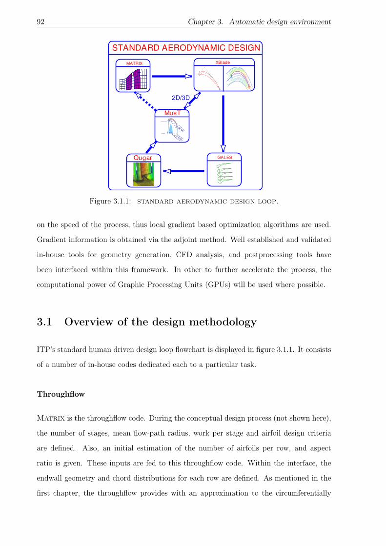
92 Chapter 3. Automatic design environment
MATRIX
MusT
XBlade
GALESQugar
STANDARD AERODYNAMIC DESIGN
2D/3D
Figure 3.1.1: standard aerodynamic design loop.
on the speed of the process, thus local gradient based optimization algorithms are used.
Gradient information is obtained via the adjoint method. Well established and validated
in-house tools for geometry generation, CFD analysis, and postprocessing tools have
been interfaced within this framework. In other to further accelerate the process, the
computational power of Graphic Processing Units (GPUs) will be used where possible.
3.1 Overview of the design methodology
ITP’s standard human driven design loop flowchart is displayed in figure 3.1.1. It consists
of a number of in-house codes dedicated each to a particular task.
Throughflow
Matrix is the throughflow code. During the conceptual design process (not shown here),
the number of stages, mean flow-path radius, work per stage and airfoil design criteria
are defined. Also, an initial estimation of the number of airfoils per row, and aspect
ratio is given. These inputs are fed to this throughflow code. Within the interface, the
endwall geometry and chord distributions for each row are defined. As mentioned in the
first chapter, the throughflow provides with an approximation to the circumferentially

3.1. Overview of the design methodology 93
Figure 3.1.2: XBlade interface.
averaged flow field. In a real world design, the throughflow is used in two ways. A lead
engineer will define the flow-path by performing several multirow analyses, and give an
estimation of the chord distributions for each row. Then, the individual row designer will
use a single row though-flow to obtain boundary conditions for the airfoil generation tool
and the CFD solver.
As the design progresses, the throughflow fidelity can by increased by including
information such as geometrical blockage (having already generated some geometries),
losses and lift distribution (from CFD analyses). At the end of the design, throughflow
and multistage 3D CFD calculations should be in very good agreement.
Two dimensional airfoil definition
This is carried out with the blading program known as XBlade [124], which is a
parametric 2D airfoil design tool that uses G 3 Bézier curves, ensuring smooth velocity
distributions.
It is an interactive application, a screen-shot of the Graphical User Interface (GUI) con
be seen in figure 3.1.2. A designer can choose from several profile templates (turbine,
compressor, throat free profile, etc...), and for each select the level of complexity of the
Bézier curves, that is, number of control points. In standard design practice, of the order
of 20 sections per 3D airfoil are built within this program.
In order to rapidly assess the quality of the generated airfoils, XBlade uses Mises [125]
to compute airfoil loading, boundary layer integral parameters, and friction coefficient.
94 Chapter 3. Automatic design environment
Boundary conditions are fed by the throughflow solver for each section. The results are
computed and displayed in real time. As regular practice, speaking of LPTs, in order
to proceed to the next stage, the airfoils must fulfill certain criteria. For example, the
loading distributions must be the required ones. This is not trivial, as when designing
non-orthogonal or low aspect ratio airfoils, Mises cannot be expected to give a good
prediction, as it is a 2D analysis tool. A designer will use his experience to design a
profile whose 2D loading will result in more or less the correct one when analyzed by 3D
CFD. Another, the size of the suction side separation bubble must be minimal. Criteria
for the pressure side separation bubble can be defined depending on the design philosophy
of the particular project.
Once the sections are defined, their coordinates are exported in a proprietary format, so
that they can be read by the stacking program.
Airfoil stacking
The stacking code Gales serves two important functions. First, it defines the stacking
law to be applied to the airfoil sections. Second, it generates a Non Rational Uniform
B-Spline (NURBS) surface to be used by the mesh generation procedures.
The program can apply the stacking line in certain locations, such as leading edge, trailing
edge, center of mass, etc... which the user can select interactively. Some presets for certain
stacking shapes are available, but for more fine tuning, the user defines a spline curve
dragging control points with the mouse.
Mesh generation
Qugar [126] is meshing tool used routinely for 3D airfoil mesh generation. The two main
inputs are the surface generated by Gales and the meridional streamlines computed by
the throughflow solver, including endwall geometries. The computational domain will be
bounded by an inlet, outlet, endwall casings and the lateral passage boundaries. The inlet
and outlet can be interactively defined by the user, but they usually are set consistent
with the throughflow model. The endwalls casings are usually generated as axisymmetric,
but for specialized applications, non axisymmetries can be applied by defining a spatial
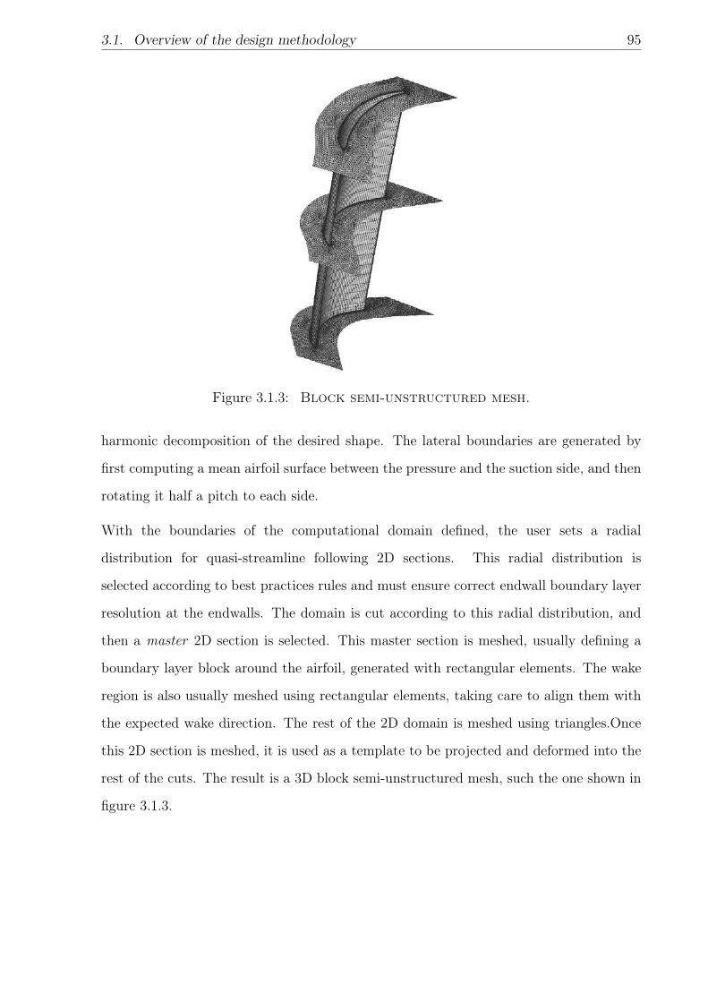
3.1. Overview of the design methodology 95
Figure 3.1.3: Block semi-unstructured mesh.
harmonic decomposition of the desired shape. The lateral boundaries are generated by
first computing a mean airfoil surface between the pressure and the suction side, and then
rotating it half a pitch to each side.
With the boundaries of the computational domain defined, the user sets a radial
distribution for quasi-streamline following 2D sections. This radial distribution is
selected according to best practices rules and must ensure correct endwall boundary layer
resolution at the endwalls. The domain is cut according to this radial distribution, and
then a master 2D section is selected. This master section is meshed, usually defining a
boundary layer block around the airfoil, generated with rectangular elements. The wake
region is also usually meshed using rectangular elements, taking care to align them with
the expected wake direction. The rest of the 2D domain is meshed using triangles.Once
this 2D section is meshed, it is used as a template to be projected and deformed into the
rest of the cuts. The result is a 3D block semi-unstructured mesh, such the one shown in
figure 3.1.3.
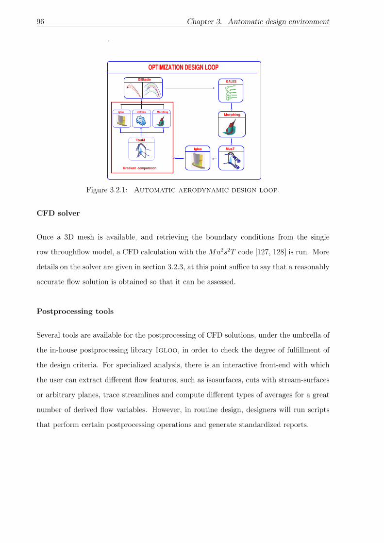
96 Chapter 3. Automatic design environment
Igloo Utilities Morphing
XBlade GALES
MusT
Morphing
Igloo
TsuM
OPTIMIZATION DESIGN LOOP
Gradient computation
Figure 3.2.1: Automatic aerodynamic design loop.
CFD solver
Once a 3D mesh is available, and retrieving the boundary conditions from the single
row throughflow model, a CFD calculation with the Mu2s2T code [127, 128] is run. More
details on the solver are given in section 3.2.3, at this point suffice to say that a reasonably
accurate flow solution is obtained so that it can be assessed.
Postprocessing tools
Several tools are available for the postprocessing of CFD solutions, under the umbrella of
the in-house postprocessing library Igloo, in order to check the degree of fulfillment of
the design criteria. For specialized analysis, there is an interactive front-end with which
the user can extract different flow features, such as isosurfaces, cuts with stream-surfaces
or arbitrary planes, trace streamlines and compute different types of averages for a great
number of derived flow variables. However, in routine design, designers will run scripts
that perform certain postprocessing operations and generate standardized reports.
3.2. Automatic design loop 97
3.2 Automatic design loop
3.2.1 Overview
The scope of the proposed design procedure is limited to the single row iterations, with
a frozen throughflow model. The modified flowchart is depicted in figure 3.2.1, where
differences with the human driven loop can be noticed. For one, the optimizer will
not interact with the throughflow.Then, assuming that the objective functionals will be
regular enough, a gradient based approach is preferred when the computational cost of
the objective function is high, as they require significantly less evaluations [129]. So, a
new block dedicated to the gradient computation stage needs to be added to the workflow
chart, comprising an adjoint solver run, and the generation of one perturbed geometry
per design parameter. At the end of each iteration, a new design vector is proposed by an
optimization routine. Finally, all the mesh generation tasks have been substituted by 3D
mesh deformation using a pseudo-Laplacian algorithm, which is significantly faster, and
can be used as long as the topology of the mesh does not change. For a reference,
generating a typical size mesh of ∼ 1.5 · 106 nodes takes 3 minutes in batch mode
(provided that an initial mesh has been generated and the procedure’s parameters have
been saved), while mesh deformation with the standard algorithm in a single CPU takes
2.5 minutes. While it does not look like much, it adds up over the sheer number of
meshes that the automatic procedure needs to generate. Furthermore, in section 4.2,
hardware and algorithmic acceleration techniques are described that dramatically increase
this difference. Figure 3.2.2 shows how a small profile deformation displaces drags all the
inner domain points.
The geometry generation tools XBlade and Gales were modified to work in batch mode,
bypassing the GUI that human designers work with. Communication with these programs
proceeds then via input/output files. Regarding the postprocessing stage, an adapted
version of the postprocessing library Igloo has been generated, in order to compute not
only the objective functions, but their sensitivities with respect to flow variables. This
will be an input for the adjoint code.
The way of interfacing to the optimizer is as follows. In order to generate a design
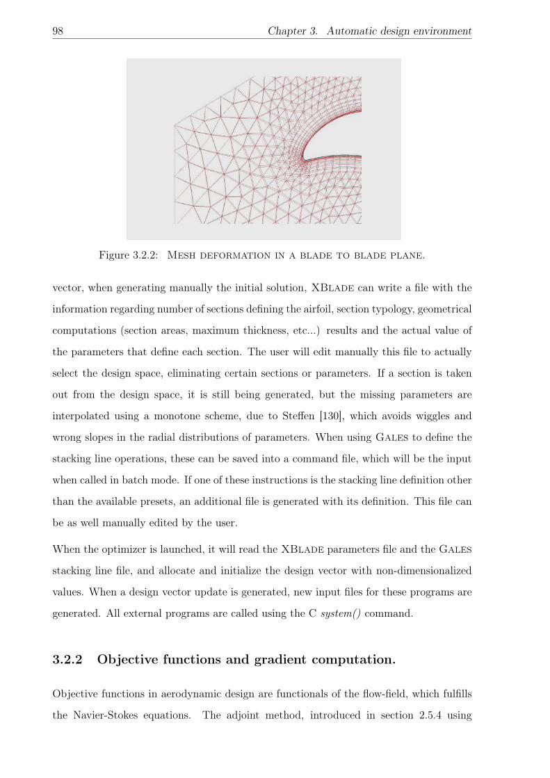
98 Chapter 3. Automatic design environment
Figure 3.2.2: Mesh deformation in a blade to blade plane.
vector, when generating manually the initial solution, XBlade can write a file with the
information regarding number of sections defining the airfoil, section typology, geometrical
computations (section areas, maximum thickness, etc...) results and the actual value of
the parameters that define each section. The user will edit manually this file to actually
select the design space, eliminating certain sections or parameters. If a section is taken
out from the design space, it is still being generated, but the missing parameters are
interpolated using a monotone scheme, due to Steffen [130], which avoids wiggles and
wrong slopes in the radial distributions of parameters. When using Gales to define the
stacking line operations, these can be saved into a command file, which will be the input
when called in batch mode. If one of these instructions is the stacking line definition other
than the available presets, an additional file is generated with its definition. This file can
be as well manually edited by the user.
When the optimizer is launched, it will read the XBlade parameters file and the Gales
stacking line file, and allocate and initialize the design vector with non-dimensionalized
values. When a design vector update is generated, new input files for these programs are
generated. All external programs are called using the C system() command.
3.2.2 Objective functions and gradient computation.
Objective functions in aerodynamic design are functionals of the flow-field, which fulfills
the Navier-Stokes equations. The adjoint method, introduced in section 2.5.4 using
3.2. Automatic design loop 99
the dual variable concept, is here particularized for the discrete RANS equations, and
explained using the Lagrange multiplier interpretation (recall from section 2.3.1 the
concept of duality of the Lagrange multipliers). The optimization problem consists in
minimizing a cost function f (u, ϕ), where the conservative variables u must fulfill the
steady state discrete RANS equations (schematically written as R (u, ϕ) = 0), and ϕ
represents the modifiable geometric parameters. The restrictions imposed by the discrete
Navier-Stokes equations can be absorbed by the functional, by multiplying each of them
by a Lagrange multiplier, v. Thus the lagrangian is built:
I (u, ϕ) = f (u, ϕ) + vT ·R (u, ϕ) (3.2.1)
Since the steady state is fulfilled, the problems of minimizing f and I are equivalent. The
gradient of I is obtained by differentiating the previous equation:
dI
dϕ=
(∂f
∂u
)T∂u
∂ϕ+∂f
∂ϕ+ vT ·
([∂R
∂u
]∂u
∂ϕ+∂R
∂ϕ
)(3.2.2)
Grouping together the terms that go with ∂u/∂ϕ, and rearranging:
dI
dϕ=
[(∂f
∂u
)T+ vT ·
[∂R
∂u
]]∂u
∂ϕ+∂f
∂ϕ+ vT · ∂R
∂ϕ(3.2.3)
The adjoint system (equation 3.2.4) appears when making the first term vanish.[∂R
∂u
]Tv +
∂f
∂u= 0 (3.2.4)
Since the analytic expression for the cost function is usually known, the cost function
sensitivity ∂f/∂u can be obtained analytically. The gradient in equation 3.2.2 can finally
be written as:
dI
dϕ= vT · ∂R
∂ϕ+∂f
∂ϕ(3.2.5)
which shows that one single solution of the adjoint equations can be used to determine
the gradient by simply multiplying the adjoint variables v by the variation of the steady
state residuals with respect to the geometric parameters ∂R/∂ϕ. This term is evaluated
using the complex variable method:
∂R
∂ϕ= lim
ε→0
= [R (u, ϕ+ iε)]
ε(3.2.6)
which is as costly as one evaluation of the discrete Navier-Stokes equations. The last term
∂f/∂ϕ is evaluated using finite differences. Recall from section 3.2.1, it is for these two
100 Chapter 3. Automatic design environment
terms that the generation of a new geometry per perturbed design parameter is needed.
Evidently, the computational time spent for this stage scales linearly with the design
space. For a usual industrial case where the number of parameters is of the order of a few
hundreds, geometry generation can take a lot computational time. This issue is addressed
in chapter 4.
3.2.3 3D unstructured RANS base solver.
The Navier-Stokes equations in conservative form for an arbitrary control volume may be
written as
d
dt
ˆΩ
Udv +
ˆΣ
[F−UV] · ndσ = S (U) (3.2.7)
where U is the vector of conservative variables, F = Fc − Fv the sum of the inviscid and
viscous fluxes (equation 3.2.9), Ω the flow domain, Σ its boundary, dA the differential area
pointing outward to the boundary, V the velocity of the boundary and S a source term
containing typically the centrifugal and Coriolis forces in a rotating frame of reference.
The solver, known as Mu2s2T , uses hybrid unstructured grids to discretize the spatial
domain that may contain cells with an arbitrary number of faces and the solution vector
is stored at the vertices of the cells. The control volume associated to a node is formed by
connecting the median dual of the cells surrounding it, using an edge-based data structure
(see figure 3.2.3). For the internal node i the semi-discrete form of the system of non-linear
equations 3.2.7 can be written using a finite volume approach as
d (ΩiUi)
dt+
nedges∑j=1
1
2(Fi + Fj) ·Aij −Dij = S (Ui) (3.2.8)
Fc · n =
ρvn
ρuvn + p · nx
ρvvn + p · ny
ρwvn + p · nz
(ρE + p) vn
, Fv · n =
0
τxn
τyn
τzn
vT · τ · n− q · n
(3.2.9)
where Ωi is the control volume, Aij is the area associated to the edge ij, 12
(Fi + Fj)
represents the inviscid and viscous fluxes through area Aij, Dij are the artificial dissipation
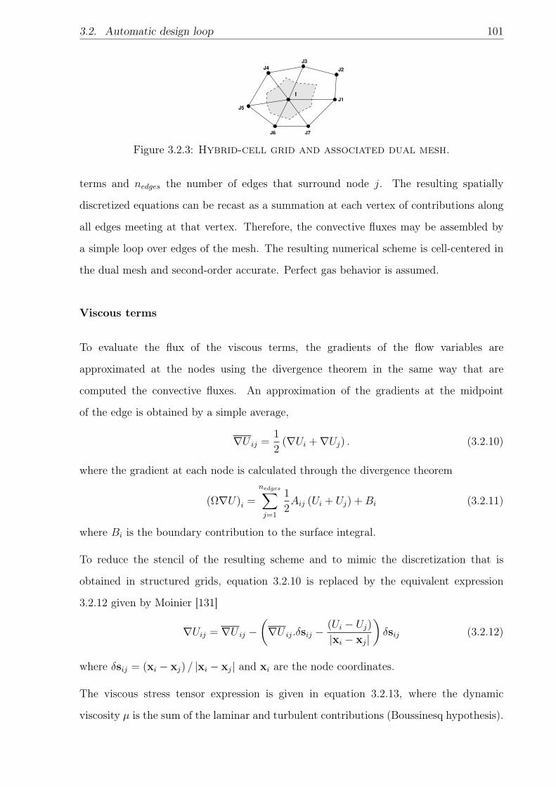
3.2. Automatic design loop 101
J1
J3
J6 J7
J5
I
J4 J2
Figure 3.2.3: Hybrid-cell grid and associated dual mesh.
terms and nedges the number of edges that surround node j. The resulting spatially
discretized equations can be recast as a summation at each vertex of contributions along
all edges meeting at that vertex. Therefore, the convective fluxes may be assembled by
a simple loop over edges of the mesh. The resulting numerical scheme is cell-centered in
the dual mesh and second-order accurate. Perfect gas behavior is assumed.
Viscous terms
To evaluate the flux of the viscous terms, the gradients of the flow variables are
approximated at the nodes using the divergence theorem in the same way that are
computed the convective fluxes. An approximation of the gradients at the midpoint
of the edge is obtained by a simple average,
∇U ij =1
2(∇Ui +∇Uj) . (3.2.10)
where the gradient at each node is calculated through the divergence theorem
(Ω∇U)i =
nedges∑j=1
1
2Aij (Ui + Uj) +Bi (3.2.11)
where Bi is the boundary contribution to the surface integral.
To reduce the stencil of the resulting scheme and to mimic the discretization that is
obtained in structured grids, equation 3.2.10 is replaced by the equivalent expression
3.2.12 given by Moinier [131]
∇Uij = ∇U ij −(∇U ij.δsij −
(Ui − Uj)|xi − xj|
)δsij (3.2.12)
where δsij = (xi − xj) / |xi − xj| and xi are the node coordinates.
The viscous stress tensor expression is given in equation 3.2.13, where the dynamic
viscosity µ is the sum of the laminar and turbulent contributions (Boussinesq hypothesis).
102 Chapter 3. Automatic design environment
The laminar part is modeled using Sutherland’s law (see equation 3.2.14), and the
turbulent part depends on the actual turbulence model selected. Several turbulence
models are implemented, including the algebraic Baldwin-Lomax model [132], the one-
equation Spalart-Allmaras [133], and several formulations of Wilcox’s k − ω model [20].
Transition prediction can be enabled using the γ −Reθ transition model by Langtry and
Menter [134, 135].
τij = µl[∂ivj + ∂jvi −2
3(∇ · v)δij] (3.2.13)
µl =1.458 · 10−6T 3/2
T + 110.4(3.2.14)
The heat conduction terms are given by:
qj = −(µlPrl
+µtPrt
)γ
γ − 1
∂ (p/ρ)
∂xj(3.2.15)
where Prl is the molecular Prandtl number, set to Pr = 0.7 and Prt is the turbulent
Prandtl number, set to Prt = 0.9.
Artificial viscosity
In addition, artificial dissipation terms are required to stabilize the solution. These terms,
Dij, are a blend of a second and fourth order operators, to capture shock waves and
remove spurious high frequency waves in smooth flow regions, respectively. The second
order derivatives are activated in the vicinity of shock waves by means of a pressure-
based sensor and locally the scheme reverts to first order in these regions. The artificial
dissipation terms can be written as
Dij = |Aij|Sij[µ
(2)ij (Uj −Ui)− µ(4)
ij (Lj − Li)]
(3.2.16)
where µ(2)ij = 0.5(µ
(2)i + µ
(2)j ) and µ
(4)ij = 0.5(µ
(4)i + µ
(4)j ) are the average of the artificial
viscosity coefficients in the nodes i and j which are given by
µ(2)i = min(ε2, k2δi), µ
(4)i = max(0, ε4 − k4δi) (3.2.17)
where δi is a pressure-based sensor
δi =
∣∣∑nedges
j=1 (pj − pi)∣∣∑nedges
j=1 (pj + pi)(3.2.18)
3.2. Automatic design loop 103
and ε2, k2, ε4 and k4 are constants. Typically ε2 = 0.5 and ε4 = 1128
. L is a pseudo-
laplacian operator constructed as a single loop over edges
L(Ui) =
nedges∑j=1
(Uj −Ui) 'nedges
4
(∆x2Uxx + ∆y2Uyy
)i
(3.2.19)
where the last approximation is only valid in regular grids. |Aij| is a 5 × 5 matrix that
plays the role of a scaling factor. If |Aij| = (|u|+ c)ijI, where I is the identity matrix, the
standard scalar formulation of the numerical dissipation terms proposed by Jameson et al.
[136], is recovered. When |Aij| is chosen as the Roe [137] matrix, the matricial form of the
artificial viscosity (Swanson and Turkel [138]) is obtained. In the latter case, block-Jacobi
preconditioning (Allmaras [? ]) has to be added to obtain reasonable convergence rates
and the pseudo-laplacian modified in the following way.
L (Ui) =
(nedges∑j=1
1
|xj − xi|
)−1 nedges∑j=1
(Uj −Ui)
Time discretization:
An explicit five-stage Runge-Kutta or an implicit inverse Euler scheme can be chosen.
Local time stepping is used to enhance the convergence acceleration, which guarantees
that disturbances will reach the inlet and outlet boundaries in a fixed number of steps
proportional to the number of cells between the inner boundary, typically the airfoil, and
the outer boundaries.
3.2.4 Adjoint solver.
The original adjoint code, named Ts2u2M , was developed by Corral and Gisbert[31], and
used for the design of non-axisymmetric end-walls. It is a hand derived discrete code,
and uses the frozen eddy viscosity assumption, that is, eddy viscosity is taken from the
non-linear base flow and turbulent transport equations are not adjoined. The derivation
of the discrete adjoint operators is now given.
104 Chapter 3. Automatic design environment
Adjoint inviscid fluxes
Recall from equation 3.2.8 that the vector of inviscid fluxes can be expressed, in an edge-
based data structure, as a sum of edge contributions, where the flux associated to the
edge ij is
FIij =
1
2
(FIi + FI
j
)σij (3.2.20)
Then the fluxes of the nodes i and j will be
FIi = FI
ij; FIj = −FI
ij (3.2.21)
Linearizing (3.2.20) yields
LFIij =
1
2
([LF I
Ui
]ui +
[LF I
Uj
]uj)σij (3.2.22)
where[LF I
Ui
]=[∂FI
i
∂Ui
]is the linear inviscid flux matrix and ui = ∂Ui/∂ϕk are the
linearized conservative variables. The flux contribution for the nodes i and j is written,
making use of equations 3.2.21 and 3.2.22: LFIi
LFIj
=σij2
[LF I
Ui
] [LF I
Uj
]−[LF I
Ui
]−[LF I
Uj
] ui
uj
(3.2.23)
where only the non-null entries of the vectors and matrices of the whole system of
equations are presented. This convention will be maintained throughout.
The adjoint inviscid flux operator is the transposed of the linear operator in Eq. 3.2.23: AFIi
AFIj
=σij2
[LF IUi
]T −[LF I
Ui
]T[LF I
Uj
]T −[LF I
Uj
]T vi
vj
(3.2.24)
The transposition of the flux matrix produces a change in the physics of the problem, as the
system matrix is now the transposed of the original one. Nevertheless, the characteristic
waves remain the same in the linear and adjoint problems, as pointed above. A change
in the sign of the derivative is also produced, therefore the waves of the adjoint problem
and these of the linear problem travel in opposite senses.
3.2. Automatic design loop 105
Adjoint viscous and artificial viscosity fluxes
When running over edges, two edge loops are required to evaluate the viscous fluxes, one
for the evaluation of the gradients of the variables, and the other for the computation
of the fluxes themselves. The gradient edge loop is easily expressed, being each edge
contribution
G(k)ij =
1
2
[IVi
]−[IVi
][IVj
]−[IVj
] ui
uj
σ(k)ij n
(k)ij (3.2.25)
where k = x, y, z stands for the coordinate directions, I is the identity matrix and Vi is
the volume associated to the i node. The adjoint gradient edge contribution is then:
AG(k)ij =
1
2
[IVi
] [IVj
]−[IVi
]−[IVj
] vivj
σ(k)ij n
(k)ij
Again this expression represents a change in the derivative sign. The resulting linearized
viscous fluxes can be schematically represented as a viscous matrix operator applied over
the gradients, LFVi
LFVj
=σij2
∑k=x,y,z
[LF V
Ui
] [LF V
Uj
]−[LF V
Ui
]−[LF V
Uj
](k)
nedges∑mn=1
G(k)mn
(3.2.26)
Transposing this expression yields the adjoint viscous fluxes: AFVi
AFVj
=∑
k=x,y,z
1
2
[IVi
] [IVj
]−[IVi
]−[IVj
]σ(k)
ij n(k)ij Λ(k) (3.2.27)
where
Λ(k) =
nedges∑mn=1
σmn2
[LF VUm
]T −[LF V
Um
]T[LF V
Un
]T −[LF V
Un
]T(k) vm
vn
(3.2.28)
This expression points out that the adjoint gradients are applied after the adjoint viscous
matrix operator. The artificial viscosity fluxes are also calculated by running two edge
loops, therefore the adjoint viscous fluxes formulation can also be used for the adjoint
artificial viscosity ones, just by substituting the appropriate operators:
106 Chapter 3. Automatic design environment
• The gradient operator (3.2.25) is substituted by a pseudo-divergence pdi
pdj
=
−[IΞi
] [IΞi
][I
Ξj
]−[I
Ξj
] ui
uj
(3.2.29)
where Ξi represents the number of edges that touch the i node.
• The viscous matrix operator in Eq. 3.2.26 is substituted by the artificial viscosity
matrix operator − [LF SUi
] [LF S
Uj
][LF S
Ui
]−[LF S
Uj
] (3.2.30)
The adjoint artificial viscosity fluxes are analogous to these in equation 3.2.27: AFSi
AFSj
=1
2
−[IΞi
] [I
Ξj
][IΞi
]−[I
Ξj
]Υ, (3.2.31)
being
Υ =
nedges∑mn=1
σmn2
− [LF SUm
]T [LF S
Um
]T[LF S
Un
]T −[LF S
Un
]T vm
vn
(3.2.32)
Adjoint boundary conditions
• Non-reflecting inlet: At the inlet, stagnation pressure pT , stagnation temperature
TT , and tangential and radial flow angles are imposed. The outgoing Riemann
invariant R− is extrapolated from inside of the computational domain in case of
subsonic flow to achieve 1D non reflectivity. In case of supersonic flow, static
pressure is also imposed, with the result that every variable is determined. Thus, for
linearized and adjoint analyses, null Dirichlet boundary conditions for every variable
are applied. The formulation is derived in appendix B.
• Non reflecting outlet: At the outlet, for a subsonic condition, static pressure ps is
imposed, and the outgoing Riemmann invariantR+ is extrapolated. For a supersonic
outlet, every variable is extrapolated both for non-linear and linear analyses. Again,
the subsonic case is expanded in appendix B.
• Wall: At walls, the no slip condition equals the flow velocity to the solid wall
velocity. Regarding the energy equation, two possibilities are considered, adiabatic
3.2. Automatic design loop 107
walls (no temperature gradient) or imposed temperature Tw. See appendix B for
the full derivation.
• Time integration: For this step, the Runge-Kutta operator, which is linear, is
adjoined. The rate of convergence should be the same as in the non-linear solution.
That this is so is shown in section 4.1.1.
Recall that the adjoint variables are forced by the objective function’s flow sensitivity
with constant geometry. This forcing is derived analytically for each of the implemented
options and computed with postprocessing software developed ad hoc. A catalogue of
implemented objective and constraint functions, with their corresponding forcings can be
found in appendix A. In order to compute the partial derivative of the objective function
and equation residuals with respect to the design vector, as many perturbed geometries as
design parameters have to be generated and postprocessed. The derivatives of geometry
dependent functionals are then computed by finite differences.
3.2.5 Scalarization approach and constraint treatment.
A general case requires of the computation of several sub-objectives and constraints.
Most of them will be functions of the fluid state, but some will only depend on the
geometry. Individual sub-objectives fk can be aggregated into a single function using
weighted exponential sums or the weighted exponential criterion, both described in section
2.4.2.
Regarding the constraint treatment, assuming an inequality constraint formulated as in
equation 3.2.33, different methods are available:
φ = g/glimit − 1 (3.2.33)
• Penalty function: The constraint contribution φ is aggregated to the total objective
function via a penalty function G(x), which is greater than zero and monotonously
increasing for x > 0 and null for x ≤ 0. Equality constraints are handled by adding
contributions at both sides of zero. An exponential function (equation 3.2.34) is
108 Chapter 3. Automatic design environment
chosen, with both function value and first derivative zero at the origin, so that it is
continuously differentiable. Both amplitude and growth rate can be modulated.
G(φ) = A [cosh(Bφ)− 1] (3.2.34)
This method can be used for both flow dependent or geometry dependent
constraints, but has been proven not very effective for the latter. For flow
constraints, the contributions to the total adjoint forcing are computed by applying
the chain rule to equations 3.2.34, 3.2.33, and the definition of the actual constraint.
• Optimizer handling method: Each of the algorithms described in section 3.2.6 have
a built-in constraint handling method. Geometry constraints are straightforward
to deal with using this approach. Flow constraints need the computation of an
additional adjoint solution. In order to minimize computational time, for flow
constraints the penalty function method would be favored, but as will be seen in
section 4.2, an adjoint solver run does not penalize total iteration time significantly.
Thus, having the optimizer handle flow constraints need not be dismissed entirely.
• Hard constraint handling: Used only with geometry constraints when the aim is
to prevent infeasible geometries from being generated. This approach is used by
[139], where the authors start from a feasible geometry and project each update
vector in the subspace of feasible movement. In this work, a requirement is that
the initial solution may not be feasible, so instead of projecting the update vector,
the actual design vector is modified within a root finding procedure. The upper
level optimization routine is not aware of this, but within one function called by
the optimizer, a non-linear system of equations solver modifies the design vector so
that it fulfills the equality constraints and the active (read unfulfilled) inequality
constraints. This is a hard coded (that is, not an external library) Broyden solver
assisted with a line search. Equality constraints are straightforward to treat this
way, while for inequality constraints, the piecewise defined penalty function allows
to discriminate when they are fulfilled. When imposing thickness or area related
constraints, this is the method of choice, not only because it was found to work best,
but for other reason. An aerodynamic designer cares mostly about phenomena
occurring at the suction side. When fulfilling thickness constraints he will only
3.3. Generalized adjoint analysis. 109
modify the pressure side, so as not to deteriorate suction side performance. This
constraint handling method is the only way to artificially reduce the design space
size during the optimization for specific constraints, and it works by reading an
additional file with the list of parameters that are allowed to change to fulfill the
corresponding constraint.
3.2.6 Optimization algorithms.
Several optimization software libraries have been tested during the course of this thesis,
and after evaluation, two are the ones that have been adopted in the current working
version of the design environment. One is IpOpt, an open source library implementing
an interior point method, mentioned in section 2.3.2.2. This library has proved to be
robust and efficient, and is generally the choice unless some constraints need to be treated
with the hard method described in section 3.2.5.
The other method is an in house library, Non Linear Constrained Optimization (NLCO),
developed originally by Martel [140], and modified for the needs of the work presented in
this thesis. It is a steepest descent method that shifts to a Broyden algorithm coupled
with a line search based on the Pschenichny penalty function. Nonlinear equality and
inequality constraints can be treated with the Lagrange multiplier method. However, the
hard constraint handling capability has been added. It is the method of choice when this
kind of constraints need to be enforced, otherwise, IpOpt is a faster converging method.
Even though IpOpt is open source, the modifications required for the implementation of
hard constraints where of such magnitude that did not guarantee the correct function of
the software.
3.3 Generalized adjoint analysis.
Adjoint variables are not mere mathematical artifices, insight can be gained out of their
analysis. A theoretical framework for their interpretation has been proposed by Shankaran
et al. [141], according to which, an adjoint variable signals the needed variation on physical
variables in order to improve the objective functional. For example, considering a loss
110 Chapter 3. Automatic design environment
minimization objective, if in a flow region the adjoint density is negative, a decrease in
the physical density leads to lower losses.
The usefulness of this approach is however limited if conservative variables are used
with this aim, since other more physically meaningful variables are preferred by human
designers. For example, if a designer decided to modify the total energy ρE in a flow
region, he would not know immediately what geometrical changes to apply. But if we
were speaking about pressure or velocity, the necessary modifications would be easily
guessed.
The idea is that if the correlation between variations of a flow variable and geometrical
changes is high, the adjoint of that variable will inform of the changes to be made in order
to control another variable whose relationship to the design parameters is uncertain.
Given a magnitude φ derived from the conservative flow variables, its sensitivity is derived
as:
δφ =∂φ
∂u
T
· δu (3.3.1)
Its adjoint counterpart, w, may be computed solving the associated adjoint equation,
where Rφ is the corresponding flux residual for the new variable:
w∂Rφ
∂φ=∂I
∂φ(3.3.2)
Applying the chain rule, we get:
w∂Rφ
∂R
∂R
∂u
du
dφ=
(∂I
∂u
du
dφ
)T (w∂Rφ
∂R
)∂R
∂u=
(∂I
∂u
)T(3.3.3)
Since vT = w · ∂Rφ/∂R, the above equation may be rewritten as:
w = vT∂R
∂Rφ
(3.3.4)
Note that this is a contravariant transformation in flux coordinates, while the
direct sensitivity computation was a covariant transformation in conservative variables
coordinates.
The next step is to derive the flux transformation. In equation 3.3.5, the chain rule is
applied to decompose the residual sensitivity ∂R/∂u in three terms, namely the sought
for flux transformation, the new flux, and the variable transformation. Given that the
residual of the equation associated toφ is a scalar function of a scalar, both transformations
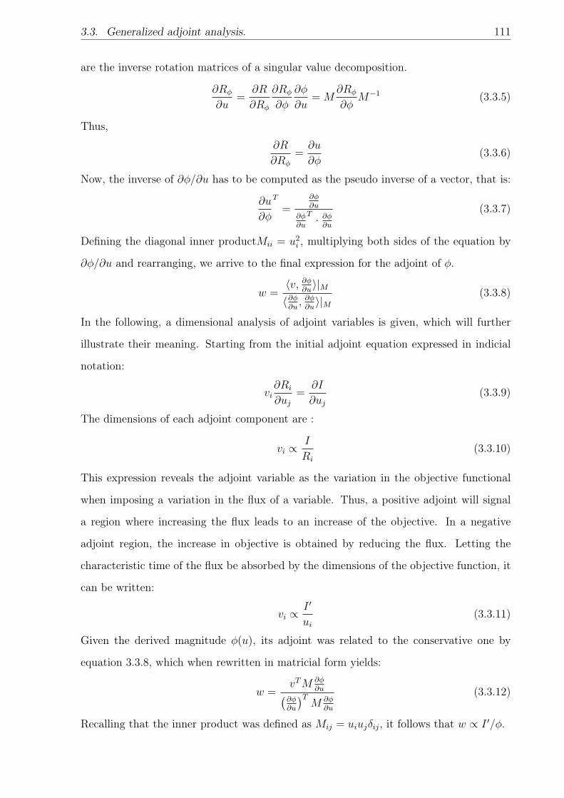
3.3. Generalized adjoint analysis. 111
are the inverse rotation matrices of a singular value decomposition.
∂Rφ
∂u=
∂R
∂Rφ
∂Rφ
∂φ
∂φ
∂u= M
∂Rφ
∂φM−1 (3.3.5)
Thus,
∂R
∂Rφ
=∂u
∂φ(3.3.6)
Now, the inverse of ∂φ/∂u has to be computed as the pseudo inverse of a vector, that is:
∂u
∂φ
T
=∂φ∂u
∂φ∂u
T · ∂φ∂u
(3.3.7)
Defining the diagonal inner productMii = u2i , multiplying both sides of the equation by
∂φ/∂u and rearranging, we arrive to the final expression for the adjoint of φ.
w =〈v, ∂φ
∂u〉|M
〈∂φ∂u, ∂φ∂u〉|M
(3.3.8)
In the following, a dimensional analysis of adjoint variables is given, which will further
illustrate their meaning. Starting from the initial adjoint equation expressed in indicial
notation:
vi∂Ri
∂uj=
∂I
∂uj(3.3.9)
The dimensions of each adjoint component are :
vi ∝I
Ri
(3.3.10)
This expression reveals the adjoint variable as the variation in the objective functional
when imposing a variation in the flux of a variable. Thus, a positive adjoint will signal
a region where increasing the flux leads to an increase of the objective. In a negative
adjoint region, the increase in objective is obtained by reducing the flux. Letting the
characteristic time of the flux be absorbed by the dimensions of the objective function, it
can be written:
vi ∝I ′
ui(3.3.11)
Given the derived magnitude φ(u), its adjoint was related to the conservative one by
equation 3.3.8, which when rewritten in matricial form yields:
w =vTM ∂φ
∂u(∂φ∂u
)TM ∂φ
∂u
(3.3.12)
Recalling that the inner product was defined as Mij = uiujδij, it follows that w ∝ I ′/φ.

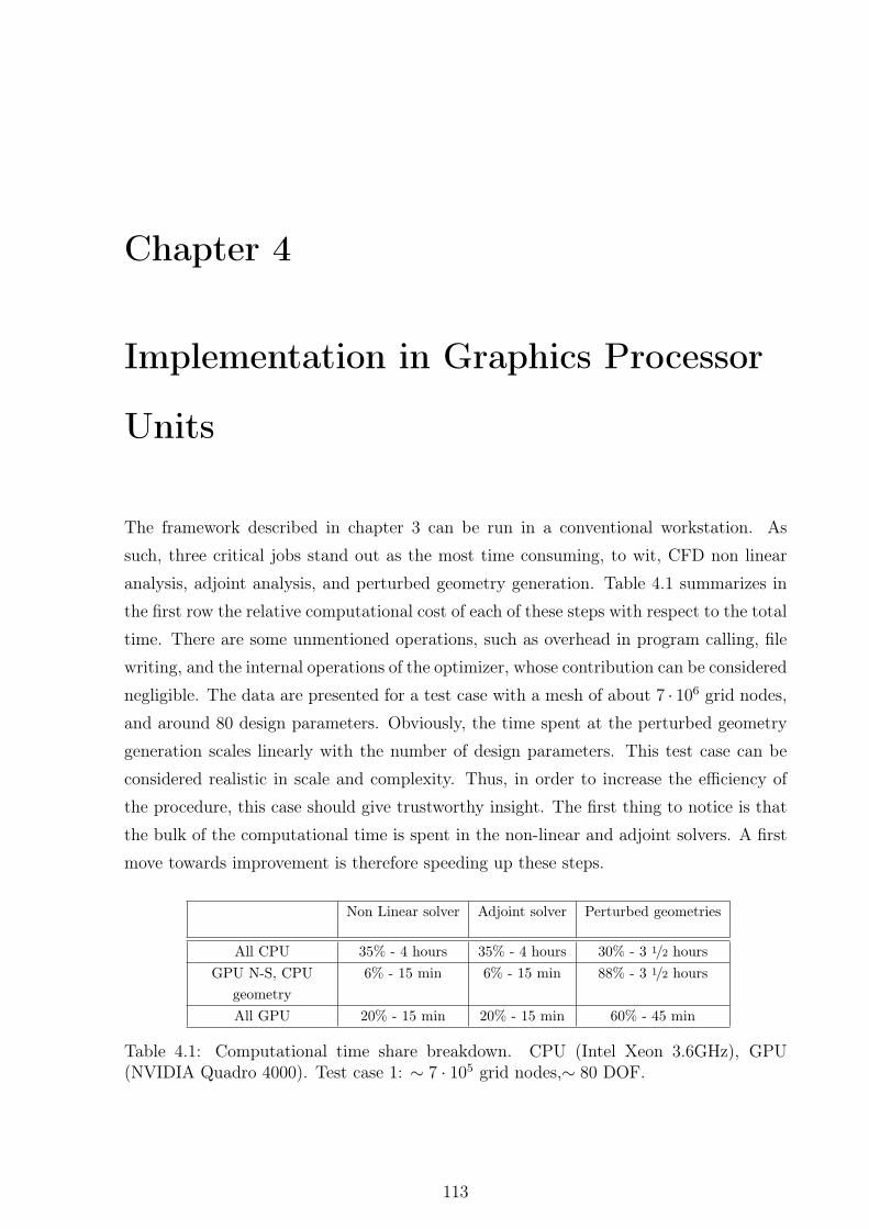
Chapter 4
Implementation in Graphics Processor
Units
The framework described in chapter 3 can be run in a conventional workstation. As
such, three critical jobs stand out as the most time consuming, to wit, CFD non linear
analysis, adjoint analysis, and perturbed geometry generation. Table 4.1 summarizes in
the first row the relative computational cost of each of these steps with respect to the total
time. There are some unmentioned operations, such as overhead in program calling, file
writing, and the internal operations of the optimizer, whose contribution can be considered
negligible. The data are presented for a test case with a mesh of about 7 · 106 grid nodes,
and around 80 design parameters. Obviously, the time spent at the perturbed geometry
generation scales linearly with the number of design parameters. This test case can be
considered realistic in scale and complexity. Thus, in order to increase the efficiency of
the procedure, this case should give trustworthy insight. The first thing to notice is that
the bulk of the computational time is spent in the non-linear and adjoint solvers. A first
move towards improvement is therefore speeding up these steps.
Non Linear solver Adjoint solver Perturbed geometries
All CPU 35% - 4 hours 35% - 4 hours 30% - 3 1/2 hoursGPU N-S, CPU
geometry6% - 15 min 6% - 15 min 88% - 3 1/2 hours
All GPU 20% - 15 min 20% - 15 min 60% - 45 min
Table 4.1: Computational time share breakdown. CPU (Intel Xeon 3.6GHz), GPU(NVIDIA Quadro 4000). Test case 1: ∼ 7 · 105 grid nodes,∼ 80 DOF.
113
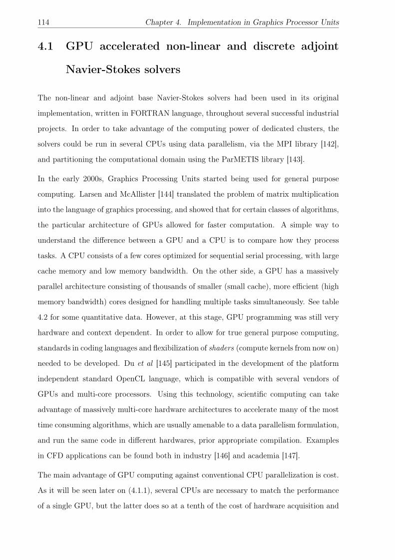
114 Chapter 4. Implementation in Graphics Processor Units
4.1 GPU accelerated non-linear and discrete adjoint
Navier-Stokes solvers
The non-linear and adjoint base Navier-Stokes solvers had been used in its original
implementation, written in FORTRAN language, throughout several successful industrial
projects. In order to take advantage of the computing power of dedicated clusters, the
solvers could be run in several CPUs using data parallelism, via the MPI library [142],
and partitioning the computational domain using the ParMETIS library [143].
In the early 2000s, Graphics Processing Units started being used for general purpose
computing. Larsen and McAllister [144] translated the problem of matrix multiplication
into the language of graphics processing, and showed that for certain classes of algorithms,
the particular architecture of GPUs allowed for faster computation. A simple way to
understand the difference between a GPU and a CPU is to compare how they process
tasks. A CPU consists of a few cores optimized for sequential serial processing, with large
cache memory and low memory bandwidth. On the other side, a GPU has a massively
parallel architecture consisting of thousands of smaller (small cache), more efficient (high
memory bandwidth) cores designed for handling multiple tasks simultaneously. See table
4.2 for some quantitative data. However, at this stage, GPU programming was still very
hardware and context dependent. In order to allow for true general purpose computing,
standards in coding languages and flexibilization of shaders (compute kernels from now on)
needed to be developed. Du et al [145] participated in the development of the platform
independent standard OpenCL language, which is compatible with several vendors of
GPUs and multi-core processors. Using this technology, scientific computing can take
advantage of massively multi-core hardware architectures to accelerate many of the most
time consuming algorithms, which are usually amenable to a data parallelism formulation,
and run the same code in different hardwares, prior appropriate compilation. Examples
in CFD applications can be found both in industry [146] and academia [147].
The main advantage of GPU computing against conventional CPU parallelization is cost.
As it will be seen later on (4.1.1), several CPUs are necessary to match the performance
of a single GPU, but the latter does so at a tenth of the cost of hardware acquisition and
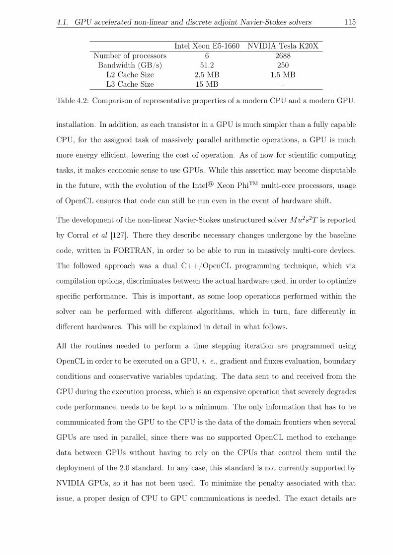
4.1. GPU accelerated non-linear and discrete adjoint Navier-Stokes solvers 115
Intel Xeon E5-1660 NVIDIA Tesla K20XNumber of processors 6 2688Bandwidth (GB/s) 51.2 250
L2 Cache Size 2.5 MB 1.5 MBL3 Cache Size 15 MB -
Table 4.2: Comparison of representative properties of a modern CPU and a modern GPU.
installation. In addition, as each transistor in a GPU is much simpler than a fully capable
CPU, for the assigned task of massively parallel arithmetic operations, a GPU is much
more energy efficient, lowering the cost of operation. As of now for scientific computing
tasks, it makes economic sense to use GPUs. While this assertion may become disputable
in the future, with the evolution of the Intel® Xeon PhiTM multi-core processors, usage
of OpenCL ensures that code can still be run even in the event of hardware shift.
The development of the non-linear Navier-Stokes unstructured solverMu2s2T is reported
by Corral et al [127]. There they describe necessary changes undergone by the baseline
code, written in FORTRAN, in order to be able to run in massively multi-core devices.
The followed approach was a dual C++/OpenCL programming technique, which via
compilation options, discriminates between the actual hardware used, in order to optimize
specific performance. This is important, as some loop operations performed within the
solver can be performed with different algorithms, which in turn, fare differently in
different hardwares. This will be explained in detail in what follows.
All the routines needed to perform a time stepping iteration are programmed using
OpenCL in order to be executed on a GPU, i. e., gradient and fluxes evaluation, boundary
conditions and conservative variables updating. The data sent to and received from the
GPU during the execution process, which is an expensive operation that severely degrades
code performance, needs to be kept to a minimum. The only information that has to be
communicated from the GPU to the CPU is the data of the domain frontiers when several
GPUs are used in parallel, since there was no supported OpenCL method to exchange
data between GPUs without having to rely on the CPUs that control them until the
deployment of the 2.0 standard. In any case, this standard is not currently supported by
NVIDIA GPUs, so it has not been used. To minimize the penalty associated with that
issue, a proper design of CPU to GPU communications is needed. The exact details are
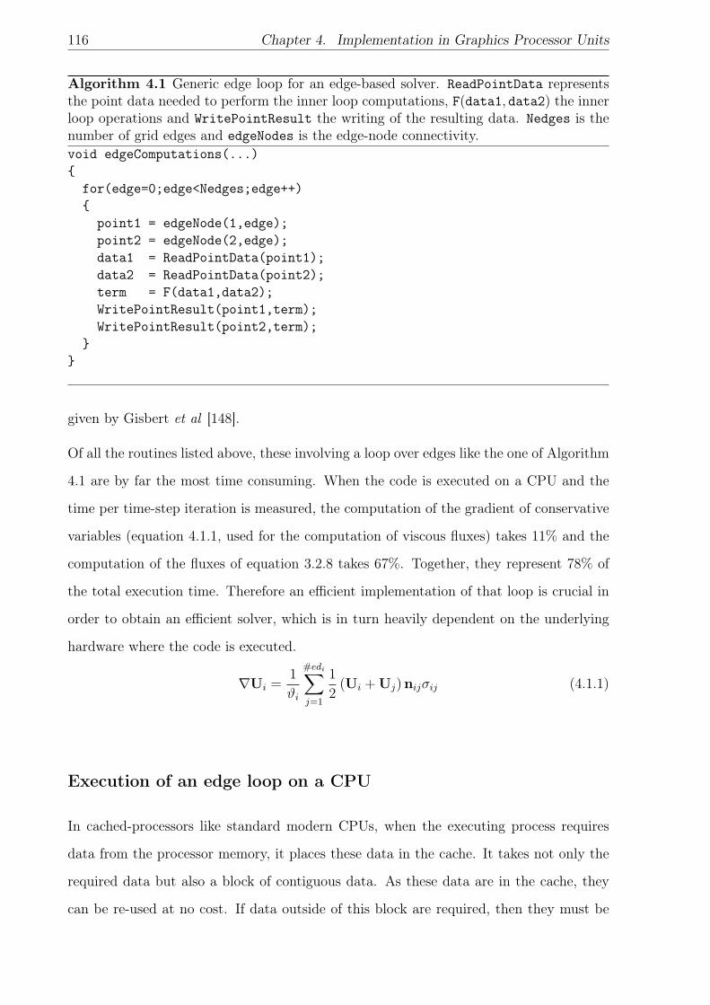
116 Chapter 4. Implementation in Graphics Processor Units
Algorithm 4.1 Generic edge loop for an edge-based solver. ReadPointData representsthe point data needed to perform the inner loop computations, F(data1, data2) the innerloop operations and WritePointResult the writing of the resulting data. Nedges is thenumber of grid edges and edgeNodes is the edge-node connectivity.void edgeComputations(...)
for(edge=0;edge<Nedges;edge++)
point1 = edgeNode(1,edge);point2 = edgeNode(2,edge);data1 = ReadPointData(point1);data2 = ReadPointData(point2);term = F(data1,data2);WritePointResult(point1,term);WritePointResult(point2,term);
given by Gisbert et al [148].
Of all the routines listed above, these involving a loop over edges like the one of Algorithm
4.1 are by far the most time consuming. When the code is executed on a CPU and the
time per time-step iteration is measured, the computation of the gradient of conservative
variables (equation 4.1.1, used for the computation of viscous fluxes) takes 11% and the
computation of the fluxes of equation 3.2.8 takes 67%. Together, they represent 78% of
the total execution time. Therefore an efficient implementation of that loop is crucial in
order to obtain an efficient solver, which is in turn heavily dependent on the underlying
hardware where the code is executed.
∇Ui =1
ϑi
#edi∑j=1
1
2(Ui + Uj) nijσij (4.1.1)
Execution of an edge loop on a CPU
In cached-processors like standard modern CPUs, when the executing process requires
data from the processor memory, it places these data in the cache. It takes not only the
required data but also a block of contiguous data. As these data are in the cache, they
can be re-used at no cost. If data outside of this block are required, then they must be
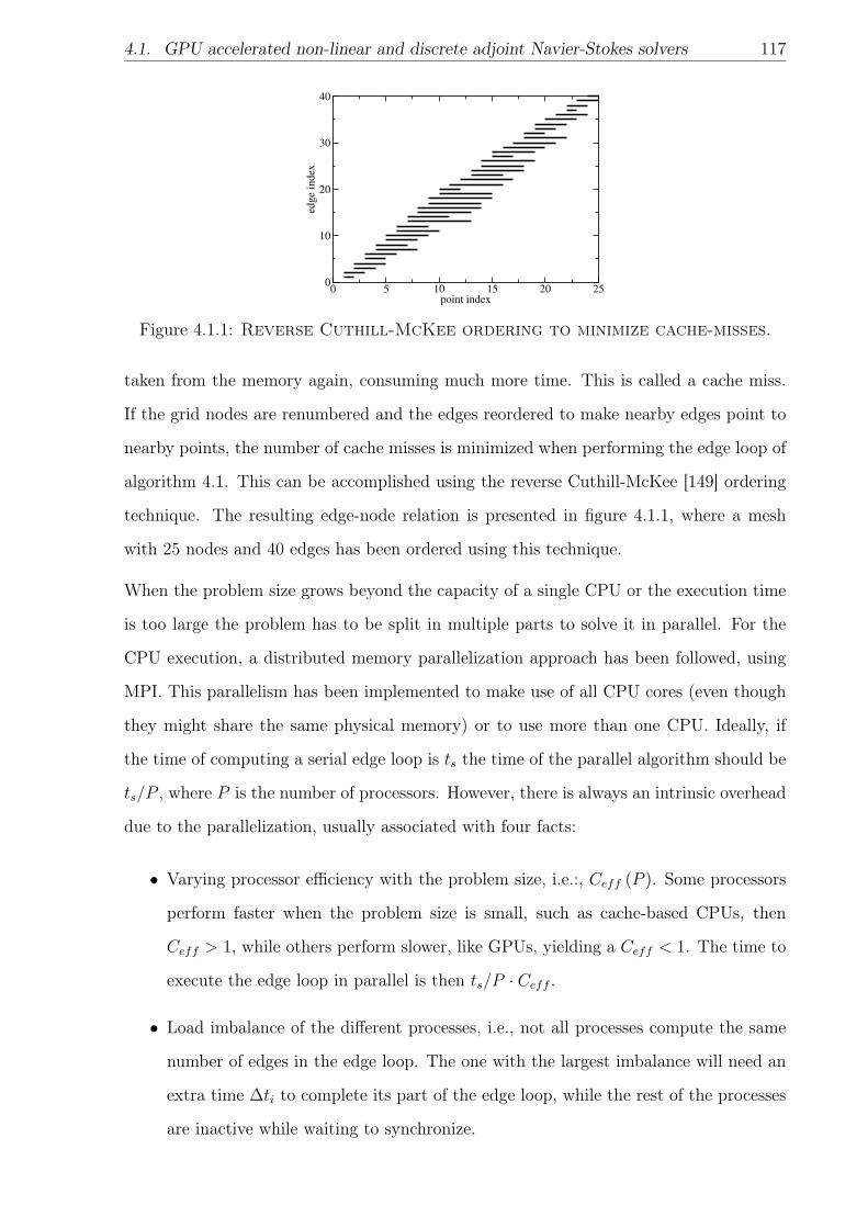
4.1. GPU accelerated non-linear and discrete adjoint Navier-Stokes solvers 117
0 5 10 15 20 25point index
0
10
20
30
40
edge
index
Figure 4.1.1: Reverse Cuthill-McKee ordering to minimize cache-misses.
taken from the memory again, consuming much more time. This is called a cache miss.
If the grid nodes are renumbered and the edges reordered to make nearby edges point to
nearby points, the number of cache misses is minimized when performing the edge loop of
algorithm 4.1. This can be accomplished using the reverse Cuthill-McKee [149] ordering
technique. The resulting edge-node relation is presented in figure 4.1.1, where a mesh
with 25 nodes and 40 edges has been ordered using this technique.
When the problem size grows beyond the capacity of a single CPU or the execution time
is too large the problem has to be split in multiple parts to solve it in parallel. For the
CPU execution, a distributed memory parallelization approach has been followed, using
MPI. This parallelism has been implemented to make use of all CPU cores (even though
they might share the same physical memory) or to use more than one CPU. Ideally, if
the time of computing a serial edge loop is ts the time of the parallel algorithm should be
ts/P , where P is the number of processors. However, there is always an intrinsic overhead
due to the parallelization, usually associated with four facts:
• Varying processor efficiency with the problem size, i.e.:, Ceff (P ). Some processors
perform faster when the problem size is small, such as cache-based CPUs, then
Ceff > 1, while others perform slower, like GPUs, yielding a Ceff < 1. The time to
execute the edge loop in parallel is then ts/P · Ceff .
• Load imbalance of the different processes, i.e., not all processes compute the same
number of edges in the edge loop. The one with the largest imbalance will need an
extra time ∆ti to complete its part of the edge loop, while the rest of the processes
are inactive while waiting to synchronize.
118 Chapter 4. Implementation in Graphics Processor Units
• Computation overhead, i.e., the extra-cost associated with the fact of splitting the
edge loop computation across several processors. The edges belonging to the parallel
domain frontier are computed twice, once for each parallel domain. Therefore, if Ei
is the number of edges for sub-domain i, the computation overhead is expressed as
Coh =
∑Ni=1 EiEs
= 1 +EfEs
being N the number of parallel sub-domains, Ef the number of parallel frontier
edges and Es the number of edges of the entire fluid domain.
• Communication overhead, i.e., the time spent exchanging data among parallel
processes, tc. The larger tc the worse the parallel performance.
Considering these factors, the actual parallel speed-up, Sa, defined as the relation between
the serial and the parallel execution of the edge loop, is
Sa =ts
tsP
CohCeff
+ ∆ti + tc
(4.1.2)
The ratio between the actual and the ideal speed-up, P , is the parallel efficiency
ξ =1
CohCeff
+
(∆tits
+tcts
)P
(4.1.3)
This expression highlights various mechanisms to increase parallel efficiency:
• Increase ts by solving larger problems (the so called weak parallel scaling) and
ensuring that ∆ti/ts and tc/ts decrease with the problem size by choosing a proper
partitioning algorithm that minimizes the load imbalance and the size of the parallel
sub-domain frontiers. In this work an efficient load balancing is achieved by using
the METIS library, which provides methods to split a given edge graph in properly
balanced sub-graphs minimizing the size of the domain frontiers (see figure 4.1.2).
This in turn reduces the computation overhead Coh which is proportional to the
number of frontier edges Ef .
• Use processors whose Ceff > 1 when the problem memory size decreases, like cache-
based CPUs. When the problem size is small enough to fit inside the cache the
4.1. GPU accelerated non-linear and discrete adjoint Navier-Stokes solvers 119
number of cache misses is zero and memory access much faster than for the larger
serial problem. However, this effect is barely noticeable for most CPUs.
• Limit the communication overhead tc. The communication time is the sum of the
network latency time tl, i.e., the time needed to establish the communication, and
the time effectively spent sending the message, which is proportional to the message
size M and inversely proportional to the network bandwidth BW :
tc = tl +M
BW
From the hardware point of view a low-latency, high bandwidth network is desired.
Once BW is fixed, there is still room for improvement, by either reducing the
message size by minimizing the frontier size, or with an appropriate design of
the communication strategy. Some MPI implementations enable the possibility
of overlapping communication and computation during the execution, by using the
so-called non-blocking or asynchronous communications. The parallel sub-domain
edge loop is then split into two parts to obtain correct results. The first part contains
all those inner domain edges, i.e., edges that do not need to exchange information
with the neighboring domains to produce correct results. The second part of the
edge loop contains only frontier edges. The communication is started before the
execution of the first edge loop and must be completed before the second part of
the edge loop is executed. In that case the effective communication time is
tceff = tl + max (0, tc − tloop)
As long as the cost of computing the contributions of the inner-domain edges is
greater than the cost of communicating the parallel frontier data the effective
communication time will almost vanish, which in turn increases the parallel
efficiency.
Execution of an edge loop on a GPU
Execution in a GPU is intrinsically parallel, and falls within the shared memory paradigm,
where all processors share the same memory space. In a GPU, literally thousands of
threads can be executed simultaneously, and all access the same physical memory at a
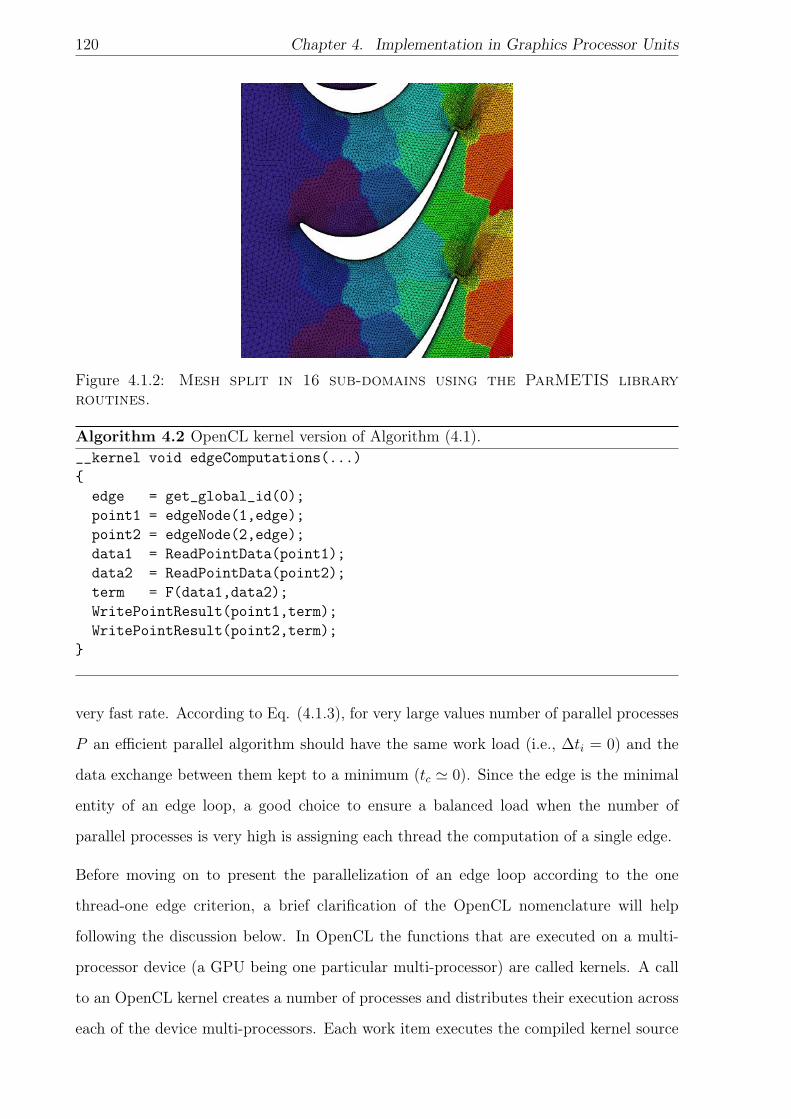
120 Chapter 4. Implementation in Graphics Processor Units
Figure 4.1.2: Mesh split in 16 sub-domains using the ParMETIS libraryroutines.
Algorithm 4.2 OpenCL kernel version of Algorithm (4.1).__kernel void edgeComputations(...)
edge = get_global_id(0);point1 = edgeNode(1,edge);point2 = edgeNode(2,edge);data1 = ReadPointData(point1);data2 = ReadPointData(point2);term = F(data1,data2);WritePointResult(point1,term);WritePointResult(point2,term);
very fast rate. According to Eq. (4.1.3), for very large values number of parallel processes
P an efficient parallel algorithm should have the same work load (i.e., ∆ti = 0) and the
data exchange between them kept to a minimum (tc ' 0). Since the edge is the minimal
entity of an edge loop, a good choice to ensure a balanced load when the number of
parallel processes is very high is assigning each thread the computation of a single edge.
Before moving on to present the parallelization of an edge loop according to the one
thread-one edge criterion, a brief clarification of the OpenCL nomenclature will help
following the discussion below. In OpenCL the functions that are executed on a multi-
processor device (a GPU being one particular multi-processor) are called kernels. A call
to an OpenCL kernel creates a number of processes and distributes their execution across
each of the device multi-processors. Each work item executes the compiled kernel source
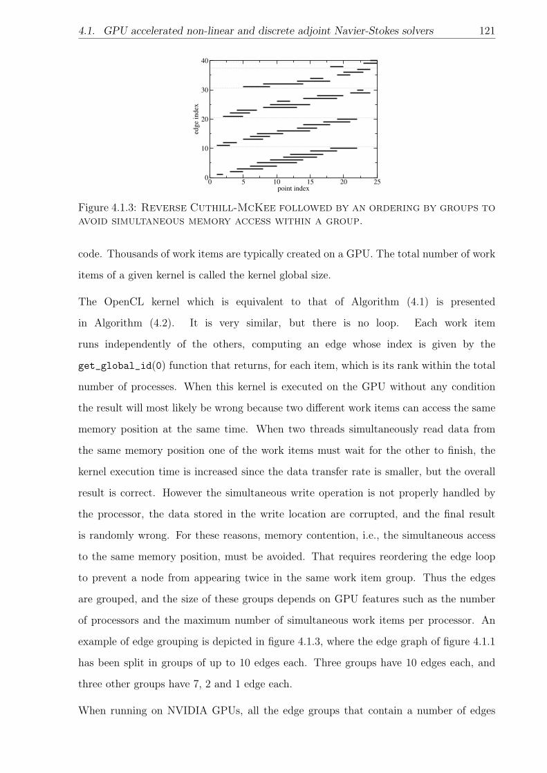
4.1. GPU accelerated non-linear and discrete adjoint Navier-Stokes solvers 121
0 5 10 15 20 25point index
0
10
20
30
40
edge
index
Figure 4.1.3: Reverse Cuthill-McKee followed by an ordering by groups toavoid simultaneous memory access within a group.
code. Thousands of work items are typically created on a GPU. The total number of work
items of a given kernel is called the kernel global size.
The OpenCL kernel which is equivalent to that of Algorithm (4.1) is presented
in Algorithm (4.2). It is very similar, but there is no loop. Each work item
runs independently of the others, computing an edge whose index is given by the
get_global_id(0) function that returns, for each item, which is its rank within the total
number of processes. When this kernel is executed on the GPU without any condition
the result will most likely be wrong because two different work items can access the same
memory position at the same time. When two threads simultaneously read data from
the same memory position one of the work items must wait for the other to finish, the
kernel execution time is increased since the data transfer rate is smaller, but the overall
result is correct. However the simultaneous write operation is not properly handled by
the processor, the data stored in the write location are corrupted, and the final result
is randomly wrong. For these reasons, memory contention, i.e., the simultaneous access
to the same memory position, must be avoided. That requires reordering the edge loop
to prevent a node from appearing twice in the same work item group. Thus the edges
are grouped, and the size of these groups depends on GPU features such as the number
of processors and the maximum number of simultaneous work items per processor. An
example of edge grouping is depicted in figure 4.1.3, where the edge graph of figure 4.1.1
has been split in groups of up to 10 edges each. Three groups have 10 edges each, and
three other groups have 7, 2 and 1 edge each.
When running on NVIDIA GPUs, all the edge groups that contain a number of edges
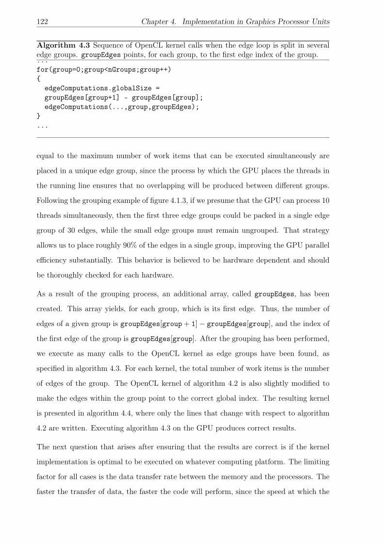
122 Chapter 4. Implementation in Graphics Processor Units
Algorithm 4.3 Sequence of OpenCL kernel calls when the edge loop is split in severaledge groups. groupEdges points, for each group, to the first edge index of the group....for(group=0;group<nGroups;group++)
edgeComputations.globalSize =groupEdges[group+1] - groupEdges[group];edgeComputations(...,group,groupEdges);
...
equal to the maximum number of work items that can be executed simultaneously are
placed in a unique edge group, since the process by which the GPU places the threads in
the running line ensures that no overlapping will be produced between different groups.
Following the grouping example of figure 4.1.3, if we presume that the GPU can process 10
threads simultaneously, then the first three edge groups could be packed in a single edge
group of 30 edges, while the small edge groups must remain ungrouped. That strategy
allows us to place roughly 90% of the edges in a single group, improving the GPU parallel
efficiency substantially. This behavior is believed to be hardware dependent and should
be thoroughly checked for each hardware.
As a result of the grouping process, an additional array, called groupEdges, has been
created. This array yields, for each group, which is its first edge. Thus, the number of
edges of a given group is groupEdges[group + 1]− groupEdges[group], and the index of
the first edge of the group is groupEdges[group]. After the grouping has been performed,
we execute as many calls to the OpenCL kernel as edge groups have been found, as
specified in algorithm 4.3. For each kernel, the total number of work items is the number
of edges of the group. The OpenCL kernel of algorithm 4.2 is also slightly modified to
make the edges within the group point to the correct global index. The resulting kernel
is presented in algorithm 4.4, where only the lines that change with respect to algorithm
4.2 are written. Executing algorithm 4.3 on the GPU produces correct results.
The next question that arises after ensuring that the results are correct is if the kernel
implementation is optimal to be executed on whatever computing platform. The limiting
factor for all cases is the data transfer rate between the memory and the processors. The
faster the transfer of data, the faster the code will perform, since the speed at which the
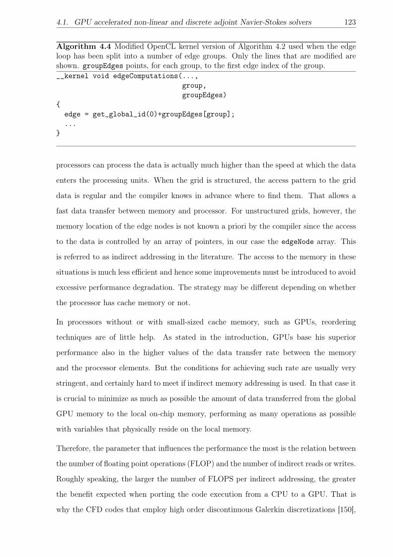
4.1. GPU accelerated non-linear and discrete adjoint Navier-Stokes solvers 123
Algorithm 4.4 Modified OpenCL kernel version of Algorithm 4.2 used when the edgeloop has been split into a number of edge groups. Only the lines that are modified areshown. groupEdges points, for each group, to the first edge index of the group.__kernel void edgeComputations(...,
group,groupEdges)
edge = get_global_id(0)+groupEdges[group];...
processors can process the data is actually much higher than the speed at which the data
enters the processing units. When the grid is structured, the access pattern to the grid
data is regular and the compiler knows in advance where to find them. That allows a
fast data transfer between memory and processor. For unstructured grids, however, the
memory location of the edge nodes is not known a priori by the compiler since the access
to the data is controlled by an array of pointers, in our case the edgeNode array. This
is referred to as indirect addressing in the literature. The access to the memory in these
situations is much less efficient and hence some improvements must be introduced to avoid
excessive performance degradation. The strategy may be different depending on whether
the processor has cache memory or not.
In processors without or with small-sized cache memory, such as GPUs, reordering
techniques are of little help. As stated in the introduction, GPUs base his superior
performance also in the higher values of the data transfer rate between the memory
and the processor elements. But the conditions for achieving such rate are usually very
stringent, and certainly hard to meet if indirect memory addressing is used. In that case it
is crucial to minimize as much as possible the amount of data transferred from the global
GPU memory to the local on-chip memory, performing as many operations as possible
with variables that physically reside on the local memory.
Therefore, the parameter that influences the performance the most is the relation between
the number of floating point operations (FLOP) and the number of indirect reads or writes.
Roughly speaking, the larger the number of FLOPS per indirect addressing, the greater
the benefit expected when porting the code execution from a CPU to a GPU. That is
why the CFD codes that employ high order discontinuous Galerkin discretizations [150],
124 Chapter 4. Implementation in Graphics Processor Units
which require performing many FLOPS per grid node, have reported the largest speed-
ups when comparing GPU and CPU execution times. But in codes where the amount of
computation per cell is not as high, like the one we are presenting here, the speed-up can
be seriously compromised if we do not pay attention to this issue. An excellent review
of the techniques employed to minimize the number of indirect addressings in edge-based
solvers can be found in Corrigan et al [151]. In order to better understand the importance
of this optimization we present here two limit cases: the gradient loop and the flux loop.
• Gradient evaluation
When the gradient evaluation of equation (4.1.1) is programmed according to
algorithm 4.2, the number of indirect addressings per edge is 6, two for reading the
variables, two for reading the gradient and two for updating it. However, the number
of operations performed inside the loop is very small, hence the performance of the
loop is completely controlled by the memory access. One simple way of reducing
the number of indirect memory accesses is presented in algorithm 4.5. In this case,
the loop is performed over grid nodes, and for each node, an inner loop over all the
edges that surround it is executed. The number of indirect addressings per edge in
this case has been reduced to one, for reading the variables of the neighbor node.
Since the total number of edges is now doubled (each edge is processed twice, once
per conforming node), the total number of indirect addressings has been divided by
three. When the loop is executed as an OpenCL kernel, the number of work items
is the number of grid nodes. For each node we compute the contributions of the
edges that share it, storing just the final result and not the intermediate ones as it
was done in algorithm 4.2.
To measure the performance of algorithms 4.2 and 4.5, both kernels have been
implemented and executed in a NVIDIA GeForce GTX780Ti. The original edge
loop of algorithm 4.1 has also been run in an Intel Xeon E5-1160. Thus, when the
algorithm 4.2 kernel is executed on the GPU, a speed-up of 4.5 is obtained with
respect to the edge loop executed on the CPU. If the modified algorithm 4.5 kernel
is executed on the same GPU, the speed-up is 14. The increase in speed-up is ∼ 3,
which agrees well with the reduction in the number of indirect addressings.
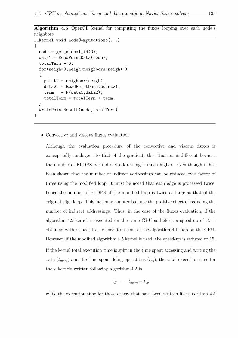
4.1. GPU accelerated non-linear and discrete adjoint Navier-Stokes solvers 125
Algorithm 4.5 OpenCL kernel for computing the fluxes looping over each node’sneighbors.__kernel void nodeComputations(...)
node = get_global_id(0);data1 = ReadPointData(node);totalTerm = 0;for(neigh=0;neigh<neighbors;neigh++)
point2 = neighbor(neigh);data2 = ReadPointData(point2);term = F(data1,data2);totalTerm = totalTerm + term;
WritePointResult(node,totalTerm)
• Convective and viscous fluxes evaluation
Although the evaluation procedure of the convective and viscous fluxes is
conceptually analogous to that of the gradient, the situation is different because
the number of FLOPS per indirect addressing is much higher. Even though it has
been shown that the number of indirect addressings can be reduced by a factor of
three using the modified loop, it must be noted that each edge is processed twice,
hence the number of FLOPS of the modified loop is twice as large as that of the
original edge loop. This fact may counter-balance the positive effect of reducing the
number of indirect addressings. Thus, in the case of the fluxes evaluation, if the
algorithm 4.2 kernel is executed on the same GPU as before, a speed-up of 19 is
obtained with respect to the execution time of the algorithm 4.1 loop on the CPU.
However, if the modified algorithm 4.5 kernel is used, the speed-up is reduced to 15.
If the kernel total execution time is split in the time spent accessing and writing the
data (tmem) and the time spent doing operations (top), the total execution time for
those kernels written following algorithm 4.2 is
tE = tmem + top
while the execution time for those others that have been written like algorithm 4.5
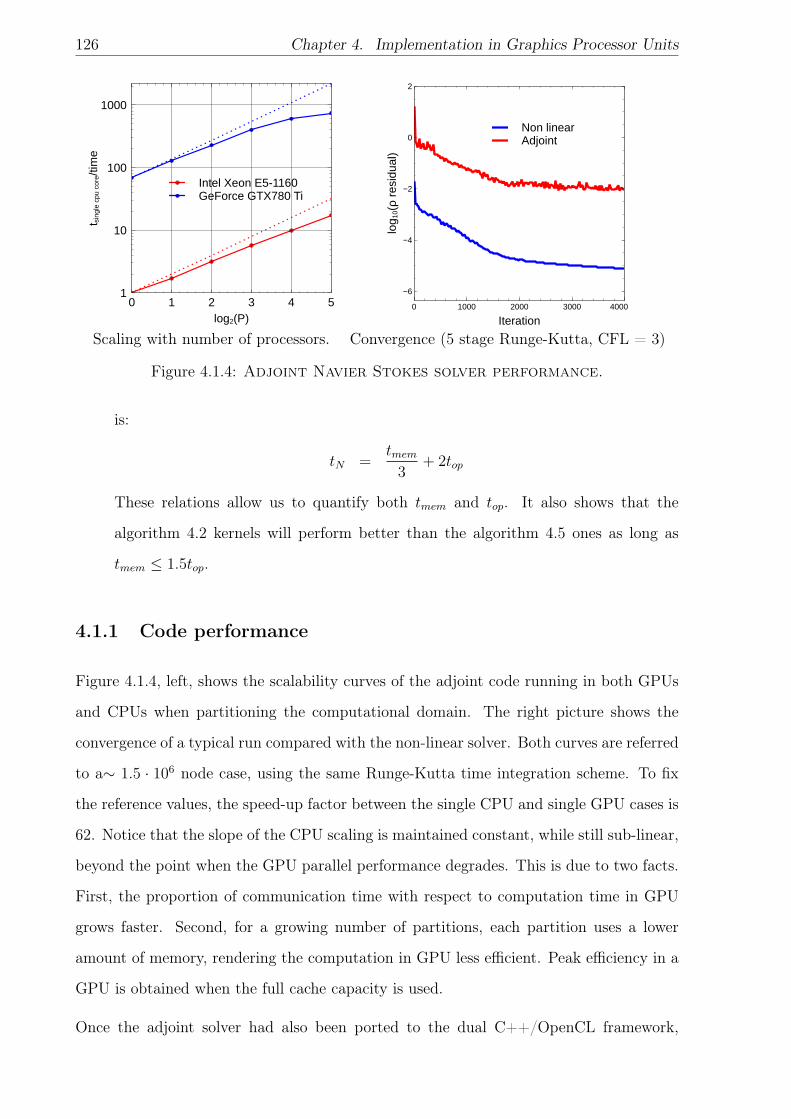
126 Chapter 4. Implementation in Graphics Processor Units
Scaling with number of processors. Convergence (5 stage Runge-Kutta, CFL = 3)
Figure 4.1.4: Adjoint Navier Stokes solver performance.
is:
tN =tmem
3+ 2top
These relations allow us to quantify both tmem and top. It also shows that the
algorithm 4.2 kernels will perform better than the algorithm 4.5 ones as long as
tmem ≤ 1.5top.
4.1.1 Code performance
Figure 4.1.4, left, shows the scalability curves of the adjoint code running in both GPUs
and CPUs when partitioning the computational domain. The right picture shows the
convergence of a typical run compared with the non-linear solver. Both curves are referred
to a∼ 1.5 · 106 node case, using the same Runge-Kutta time integration scheme. To fix
the reference values, the speed-up factor between the single CPU and single GPU cases is
62. Notice that the slope of the CPU scaling is maintained constant, while still sub-linear,
beyond the point when the GPU parallel performance degrades. This is due to two facts.
First, the proportion of communication time with respect to computation time in GPU
grows faster. Second, for a growing number of partitions, each partition uses a lower
amount of memory, rendering the computation in GPU less efficient. Peak efficiency in a
GPU is obtained when the full cache capacity is used.
Once the adjoint solver had also been ported to the dual C++/OpenCL framework,
4.2. GPU accelerated mesh deformation 127
obtaining analogous speed-ups with respect to the baseline adjoint solver when run in
GPUs, a second row can be added to Table 4.1. It turns out that the bottleneck of the
process is now on the generation of perturbed geometries.
4.2 GPU accelerated mesh deformation
As mentioned in section 3.2.1, while a mesh for the initial solution needs to be built using
the standard procedure, the automatic design procedure will only be performing mesh
deformation. A new mesh is built by projecting the old airfoil boundary into the modified
one, and applying a pseudo-Laplacian smoothing operator in the rest of the domain. The
FORTRAN code used to perform these operations, described by Contreras et al [152], has
also been rewritten to run in OpenCL devices. The smoothing operator, is formulated as:
δnewi =
δi + εn∑j=1
δjl2ij
1 + εn∑j=1
1l2ij
(4.2.1)
formalizes a spring analogy where the stiffness of the edges decreases with its length.
There, δ is a shorthand for each cartesian coordinates. This operator is qualitatively
similar to the gradient, in that it involves very few operations. Thus, the same
considerations apply. Table 4.3, presents the results of the profiling of the mesh
deformation operator, excluding the time spent in mesh reading and writing, and
boundary movement computation. Thus, when considering the scalability of the mesh
deformation process, this overhead time will contribute negatively. At the sight of it,
looping over nodes (algorithm 4.5) is less efficient than the loop ever edges (algorithm
4.1) by a small margin. Running in GPU, both loop types are accelerated, more so the
nodes loop. These result are qualitatively consistent with the results of the flow solvers,
if not quantitatively due to the simplicity of the algorithm. Recall from 4.1 that the main
source of speed-up in a GPU is their extremely high floating point operations per second
(FLOP) count. If the algorithm’s computational cost is not clearly dominated by the cost
of the floating point operations, there is less potential for speed-up.
An algorithmic improvement is described by Wang et al [153], where it is proposed that
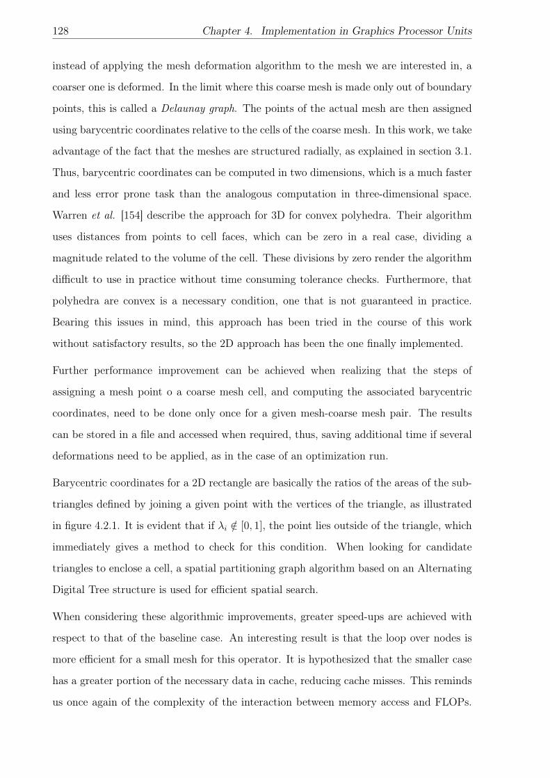
128 Chapter 4. Implementation in Graphics Processor Units
instead of applying the mesh deformation algorithm to the mesh we are interested in, a
coarser one is deformed. In the limit where this coarse mesh is made only out of boundary
points, this is called a Delaunay graph. The points of the actual mesh are then assigned
using barycentric coordinates relative to the cells of the coarse mesh. In this work, we take
advantage of the fact that the meshes are structured radially, as explained in section 3.1.
Thus, barycentric coordinates can be computed in two dimensions, which is a much faster
and less error prone task than the analogous computation in three-dimensional space.
Warren et al. [154] describe the approach for 3D for convex polyhedra. Their algorithm
uses distances from points to cell faces, which can be zero in a real case, dividing a
magnitude related to the volume of the cell. These divisions by zero render the algorithm
difficult to use in practice without time consuming tolerance checks. Furthermore, that
polyhedra are convex is a necessary condition, one that is not guaranteed in practice.
Bearing this issues in mind, this approach has been tried in the course of this work
without satisfactory results, so the 2D approach has been the one finally implemented.
Further performance improvement can be achieved when realizing that the steps of
assigning a mesh point o a coarse mesh cell, and computing the associated barycentric
coordinates, need to be done only once for a given mesh-coarse mesh pair. The results
can be stored in a file and accessed when required, thus, saving additional time if several
deformations need to be applied, as in the case of an optimization run.
Barycentric coordinates for a 2D rectangle are basically the ratios of the areas of the sub-
triangles defined by joining a given point with the vertices of the triangle, as illustrated
in figure 4.2.1. It is evident that if λi /∈ [0, 1], the point lies outside of the triangle, which
immediately gives a method to check for this condition. When looking for candidate
triangles to enclose a cell, a spatial partitioning graph algorithm based on an Alternating
Digital Tree structure is used for efficient spatial search.
When considering these algorithmic improvements, greater speed-ups are achieved with
respect to that of the baseline case. An interesting result is that the loop over nodes is
more efficient for a small mesh for this operator. It is hypothesized that the smaller case
has a greater portion of the necessary data in cache, reducing cache misses. This reminds
us once again of the complexity of the interaction between memory access and FLOPs.
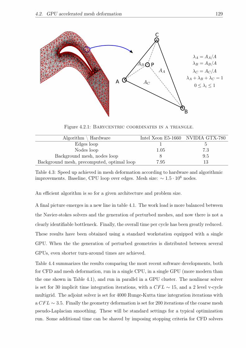
4.2. GPU accelerated mesh deformation 129
A
B
C
P
Figure 4.2.1: Barycentric coordinates in a triangle.
Algorithm \ Hardware Intel Xeon E5-1660 NVIDIA GTX-780Edges loop 1 5Nodes loop 1.05 7.3
Background mesh, nodes loop 8 9.5Background mesh, precomputed, optimal loop 7.95 13
Table 4.3: Speed up achieved in mesh deformation according to hardware and algorithmicimprovements. Baseline, CPU loop over edges. Mesh size: ∼ 1.5 · 106 nodes.
An efficient algorithm is so for a given architecture and problem size.
A final picture emerges in a new line in table 4.1. The work load is more balanced between
the Navier-stokes solvers and the generation of perturbed meshes, and now there is not a
clearly identifiable bottleneck. Finally, the overall time per cycle has been greatly reduced.
These results have been obtained using a standard workstation equipped with a single
GPU. When the the generation of perturbed geometries is distributed between several
GPUs, even shorter turn-around times are achieved.
Table 4.4 summarizes the results comparing the most recent software developments, both
for CFD and mesh deformation, run in a single CPU, in a single GPU (more modern than
the one shown in Table 4.1), and run in parallel in a GPU cluster. The nonlinear solver
is set for 30 implicit time integration iterations, with a CFL ∼ 15, and a 2 level v-cycle
multigrid. The adjoint solver is set for 4000 Runge-Kutta time integration iterations with
a CFL ∼ 3.5. Finally the geometry deformation is set for 200 iterations of the coarse mesh
pseudo-Laplacian smoothing. These will be standard settings for a typical optimization
run. Some additional time can be shaved by imposing stopping criteria for CFD solvers
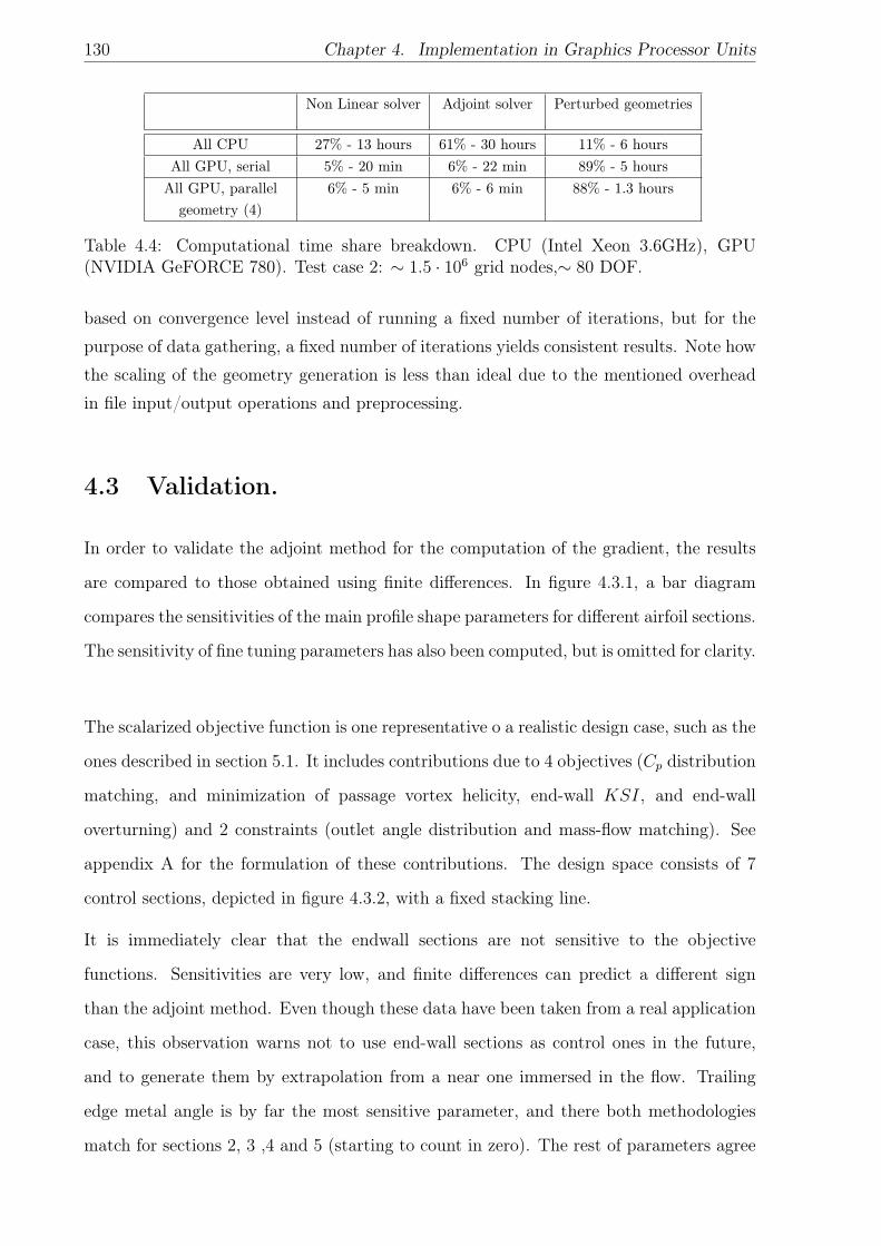
130 Chapter 4. Implementation in Graphics Processor Units
Non Linear solver Adjoint solver Perturbed geometries
All CPU 27% - 13 hours 61% - 30 hours 11% - 6 hoursAll GPU, serial 5% - 20 min 6% - 22 min 89% - 5 hours
All GPU, parallelgeometry (4)
6% - 5 min 6% - 6 min 88% - 1.3 hours
Table 4.4: Computational time share breakdown. CPU (Intel Xeon 3.6GHz), GPU(NVIDIA GeFORCE 780). Test case 2: ∼ 1.5 · 106 grid nodes,∼ 80 DOF.
based on convergence level instead of running a fixed number of iterations, but for the
purpose of data gathering, a fixed number of iterations yields consistent results. Note how
the scaling of the geometry generation is less than ideal due to the mentioned overhead
in file input/output operations and preprocessing.
4.3 Validation.
In order to validate the adjoint method for the computation of the gradient, the results
are compared to those obtained using finite differences. In figure 4.3.1, a bar diagram
compares the sensitivities of the main profile shape parameters for different airfoil sections.
The sensitivity of fine tuning parameters has also been computed, but is omitted for clarity.
The scalarized objective function is one representative o a realistic design case, such as the
ones described in section 5.1. It includes contributions due to 4 objectives (Cp distribution
matching, and minimization of passage vortex helicity, end-wall KSI, and end-wall
overturning) and 2 constraints (outlet angle distribution and mass-flow matching). See
appendix A for the formulation of these contributions. The design space consists of 7
control sections, depicted in figure 4.3.2, with a fixed stacking line.
It is immediately clear that the endwall sections are not sensitive to the objective
functions. Sensitivities are very low, and finite differences can predict a different sign
than the adjoint method. Even though these data have been taken from a real application
case, this observation warns not to use end-wall sections as control ones in the future,
and to generate them by extrapolation from a near one immersed in the flow. Trailing
edge metal angle is by far the most sensitive parameter, and there both methodologies
match for sections 2, 3 ,4 and 5 (starting to count in zero). The rest of parameters agree

4.3. Validation. 131
Figure 4.3.1: Adjoint and Finite differences sensitivity computation.
~30%
~15%
50%
~70%
~85%
100%
0%
Figure 4.3.2: design sections with representative spanwise locations.

132 Chapter 4. Implementation in Graphics Processor Units
well also for these. There is some mismatch however in section 1 and the leading edge of
section 2. The conclusion is that both methodologies are generally in good agreement.
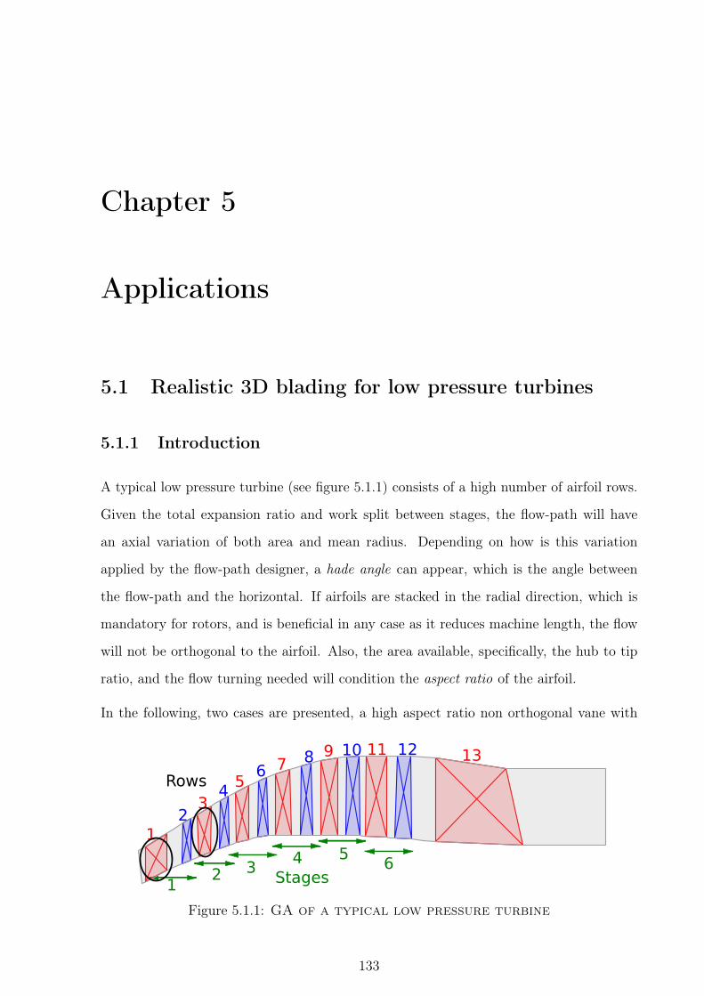
Chapter 5
Applications
5.1 Realistic 3D blading for low pressure turbines
5.1.1 Introduction
A typical low pressure turbine (see figure 5.1.1) consists of a high number of airfoil rows.
Given the total expansion ratio and work split between stages, the flow-path will have
an axial variation of both area and mean radius. Depending on how is this variation
applied by the flow-path designer, a hade angle can appear, which is the angle between
the flow-path and the horizontal. If airfoils are stacked in the radial direction, which is
mandatory for rotors, and is beneficial in any case as it reduces machine length, the flow
will not be orthogonal to the airfoil. Also, the area available, specifically, the hub to tip
ratio, and the flow turning needed will condition the aspect ratio of the airfoil.
In the following, two cases are presented, a high aspect ratio non orthogonal vane with
Figure 5.1.1: GA of a typical low pressure turbine
133
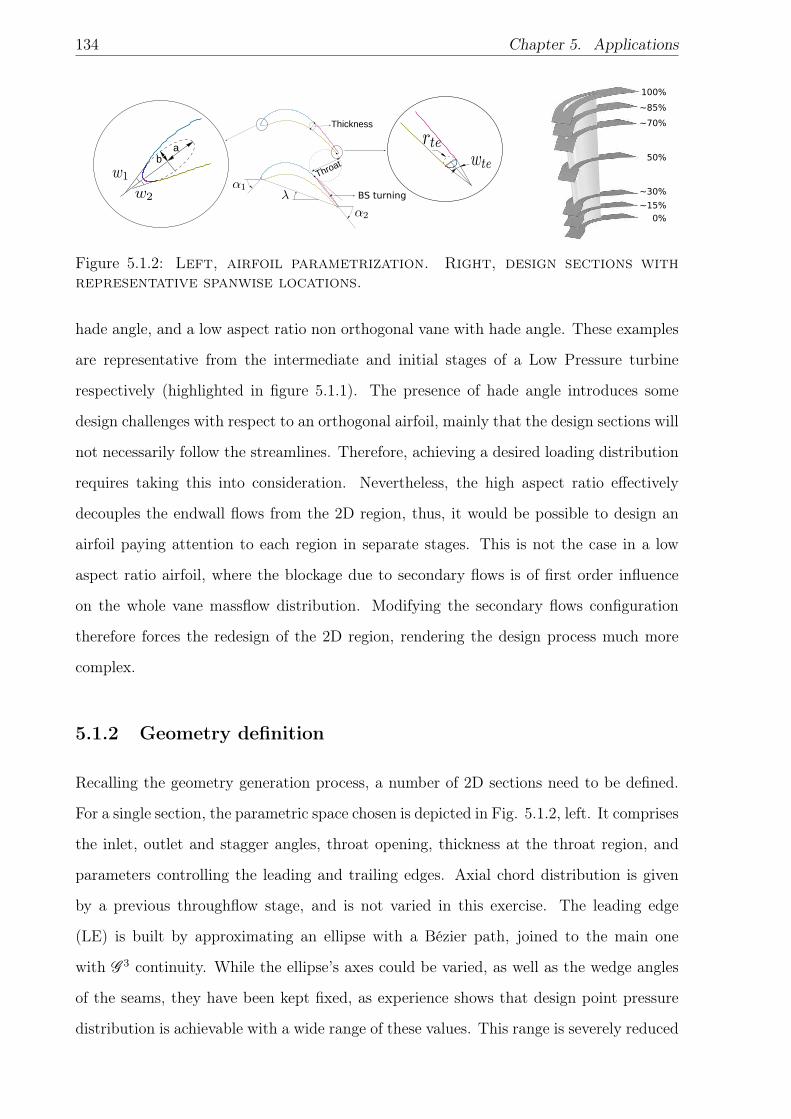
134 Chapter 5. Applications
Throat
Thickness
ab
BS turning ~30%
~15%
50%
~70%
~85%
100%
0%
Figure 5.1.2: Left, airfoil parametrization. Right, design sections withrepresentative spanwise locations.
hade angle, and a low aspect ratio non orthogonal vane with hade angle. These examples
are representative from the intermediate and initial stages of a Low Pressure turbine
respectively (highlighted in figure 5.1.1). The presence of hade angle introduces some
design challenges with respect to an orthogonal airfoil, mainly that the design sections will
not necessarily follow the streamlines. Therefore, achieving a desired loading distribution
requires taking this into consideration. Nevertheless, the high aspect ratio effectively
decouples the endwall flows from the 2D region, thus, it would be possible to design an
airfoil paying attention to each region in separate stages. This is not the case in a low
aspect ratio airfoil, where the blockage due to secondary flows is of first order influence
on the whole vane massflow distribution. Modifying the secondary flows configuration
therefore forces the redesign of the 2D region, rendering the design process much more
complex.
5.1.2 Geometry definition
Recalling the geometry generation process, a number of 2D sections need to be defined.
For a single section, the parametric space chosen is depicted in Fig. 5.1.2, left. It comprises
the inlet, outlet and stagger angles, throat opening, thickness at the throat region, and
parameters controlling the leading and trailing edges. Axial chord distribution is given
by a previous throughflow stage, and is not varied in this exercise. The leading edge
(LE) is built by approximating an ellipse with a Bézier path, joined to the main one
with G 3 continuity. While the ellipse’s axes could be varied, as well as the wedge angles
of the seams, they have been kept fixed, as experience shows that design point pressure
distribution is achievable with a wide range of these values. This range is severely reduced
5.1. Realistic 3D blading for low pressure turbines 135
when considering off-design performance, but this study is not the object of this work.
The trailing edge (TE) is similar, but using a simple circle, since the curvature continuity
is not an issue here. The TE’s radius was not allowed to vary in this case, and was set
to the minimum value defined by casting requirements. Wedge angles at the TE are also
fixed. The design system also allows to modify the location of the Bézier curve’s control
points. This provides with a great degree of fine tuning capabilities.
A total of 7 design sections, those depicted in Fig. 5.1.2 right, are used by the automatic
procedure. A human designer will select as many as he considers necessary but a
usual number is 11 sections. Additional sections in between, up to 23, are generated
interpolating the design parameters using a monotone spline scheme, as mentioned in
section 3.2.1. This scheme avoids well known oscillatory effects typical of cubic spline
interpolation. These sections are then stacked radially at the TE, and the final surface is
generated using NURBS surfaces connecting all sections.
5.1.3 Objective and constraint functions
5.1.3.1 Flow dependent functionals
A multi objective problem is posed in order to meet the multiple requirements and design
criteria for a complex component. The first objective is to match a prescribed 2D loading
distribution, CP , at the suction side, which is experimentally known to give optimum
profile losses for a given design solidity and Reynolds number. The pressure side would
be subject to other considerations, such as the separation bubble size, which are not taken
into account in this work. This is formulated as the minimization of the least squares
error between the desired Cp distribution and the actual one.
The second objective is the control of secondary flows, using three metrics. The first one
is the helicity h = ω · v (where ω = ∇× v) induced by the PS leg of the horseshoe vortex,
and the passage vortex, which happen to contribute in the same sense. Trailing edge shed
vorticity contributes in the opposite sense, but as it is an inviscid phenomenon, it cannot
be counted as a loss until full mixing has taken place. Using this metric the SS leg of the
horseshoe vortex is ignored. The second one is the minimization of mass averaged Kinetic
136 Chapter 5. Applications
Energy Losses (KSI), considering only the contributions of a certain portion of the span
near the endwalls (3D flow region). The third one is the minimization of the overturning
angle due to the pressure gradient between pressure and suction sides at the endwall.
A constraint on outlet flow angle is imposed formulated as the least squares error
minimization of the mass averaged radial angle distribution with respect to an objective
linear one defined only in the 2D region of the flow.
5.1.3.2 Geometrical constraints
Some design parameters are bounded according to design criteria. For example, outlet
metal angles should not differ too much from the expected flow ones. Throat opening
largely defines the actual flow angles, so large variations are not expected in the
bidimensional flow region, due to the constraint previously mentioned. However, in
the secondary flow regions it could vary, so bounds are set due to geometry generation
concerns.
Finally, a constraint on the radial distribution of maximum thickness is imposed by
specifying an upper and a lower limit, with the particularity that only the parameters that
affect the pressure side are modified. This reduction of the design space is built into the
root finding procedure previously mentioned. These upper and lower limits in practice
impose a certain thickness in the 2D region, which is deemed to be aerodynamically
optimal, with no pressure side separation. In the endwall region freedom is allowed in
order to tailor the secondary flow features.
5.1.3.3 Solver settings.
The solver is run with an implicit time integration scheme, and a two-level multigrid
convergence acceleration algorithm. Turbulence is treated with an algebraic model.
Boundary conditions imposed at the inlet are radial distributions of total pressure, total
temperature and flow angles. At the outlet, the radial distribution of static pressure is
specified. These data, as mentioned elsewhere, are taken from a throughflow calculation
set at the stage definition phase.

5.1. Realistic 3D blading for low pressure turbines 137
The convergence criterion established for the CFD analyses of each geometry has been
defined as the density residual going below certain threshold. This is extracted from
the analysis of the baseline geometry, as a point little before the residuals become flat.
The residuals of the modified geometries consistently fall to the same level as the initial
solution, meaning that the deformed meshes maintain high quality and that no oscillating
phenomena occur. This is to be expected, as secondary flows control aim to reduce possible
oscillation sources. Were the nature of the problem somewhat different, the definition of
convergence criteria may be a more difficult task.
The adjoint solver is run without multigrid. It also converges to flat levels, but these
depend on the intensity of the forcing term, so that a systematic definition of a threshold
level is not possible. Thus, the solver is set to run for a given number of iterations, chosen
empirically so that residuals are allowed to reach the flat region.
5.1.4 Results
The optimization solver used in this case has been the in house developed routine NLCO,
as the thickness and parameter limit constraints are imposed in a hard way. The initial
geometries are obtained by severely deforming an existing design, ensuring that this initial
solution is far away from the optimum. This way, the system will have to deal with large
geometrical changes, thus proving its robustness. Different design spaces are used for each
case, depending on what the human designer actually used. The automatic system can
be made to work with the same design space as the human driven process.
5.1.4.1 High aspect ratio, hade angle non-orthogonal vane
This case has been run considering all walls as fully turbulent, in order to test the
procedure without introducing further complexities due to the influence of a suction side
separation bubble in the loading shape. Eleven out of the about 20 parameters defining
each section are controlled by the optimizer, giving a total of 11 × 23 = 77 degrees of
freedom. The convergence of the optimization run is shown in Fig. 5.1.3, left. It has
taken roughly 2.5 days to run for 32 iterations. All functionals are normalized so that the
initial value is 1. Loading and outlet angle distribution least square errors, can potentially
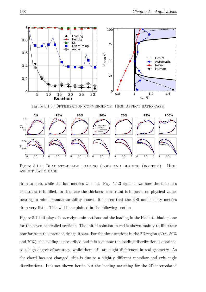
138 Chapter 5. Applications
LoadingHelicityKSIOverturningAngle
0
0.2
0.4
0.6
0.8
1
Iteration5 10 15 20 25 30
Limits
Span%
0
100
tmx /t*
0.8 1 1.2 1.4
50
25
75
LimitsAutomaticInitialHuman
Figure 5.1.3: Optimization convergence. High aspect ratio case.
0%
Cp
0
0.5
1
1.515% 30%
ObjectiveHumanAutomaticInitial
50% 70% 85% 100%
θ
0
0.02
0.04
0 0.5 1 0 0.5 1 0 0.5 1 0 0.5 1 0 0.5 1 0 0.5 1 0 0.5 1
Figure 5.1.4: Blade-to-blade loading (top) and blading (bottom). Highaspect ratio case.
drop to zero, while the loss metrics will not. Fig. 5.1.3 right shows how the thickness
constraint is fulfilled. In this case the thickness constraint is imposed on physical value,
bearing in mind manufacturability issues. It is seen that the KSI and helicity metrics
drop very little. This will be explained in the following sections.
Figure 5.1.4 displays the aerodynamic sections and the loading in the blade-to-blade plane
for the seven controlled sections. The initial solution in red is shown mainly to illustrate
how far from the intended design it was. For the three sections in the 2D region (30%, 50%
and 70%), the loading is prescribed and it is seen how the loading distribution is obtained
to a high degree of accuracy, while there still are slight differences in real geometry. As
the chord has not changed, this is due to a slightly different massflow and exit angle
distributions. It is not shown herein but the loading matching for the 2D interpolated
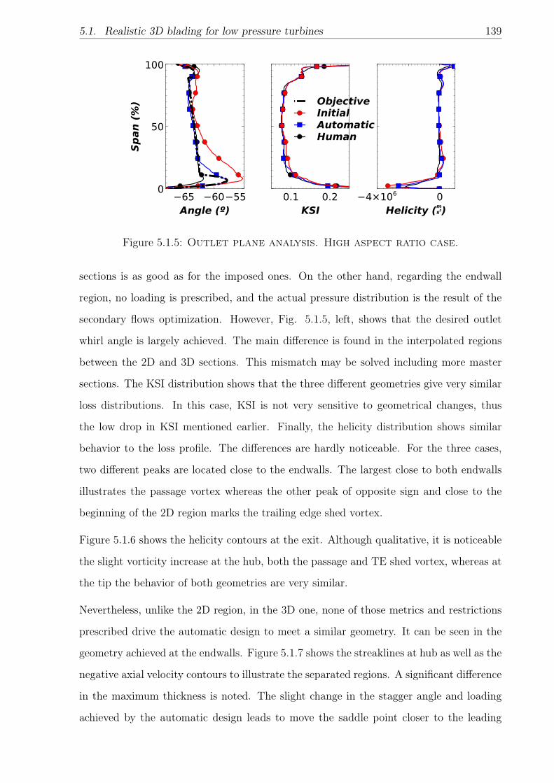
5.1. Realistic 3D blading for low pressure turbines 139
ObjectiveInitialAutomaticHuman
Span(%
)
0
50
100
Angle (º)−65 −60−55
KSI0.1 0.2
Helicity (s2m)
−4×10⁶ 0
Figure 5.1.5: Outlet plane analysis. High aspect ratio case.
sections is as good as for the imposed ones. On the other hand, regarding the endwall
region, no loading is prescribed, and the actual pressure distribution is the result of the
secondary flows optimization. However, Fig. 5.1.5, left, shows that the desired outlet
whirl angle is largely achieved. The main difference is found in the interpolated regions
between the 2D and 3D sections. This mismatch may be solved including more master
sections. The KSI distribution shows that the three different geometries give very similar
loss distributions. In this case, KSI is not very sensitive to geometrical changes, thus
the low drop in KSI mentioned earlier. Finally, the helicity distribution shows similar
behavior to the loss profile. The differences are hardly noticeable. For the three cases,
two different peaks are located close to the endwalls. The largest close to both endwalls
illustrates the passage vortex whereas the other peak of opposite sign and close to the
beginning of the 2D region marks the trailing edge shed vortex.
Figure 5.1.6 shows the helicity contours at the exit. Although qualitative, it is noticeable
the slight vorticity increase at the hub, both the passage and TE shed vortex, whereas at
the tip the behavior of both geometries are very similar.
Nevertheless, unlike the 2D region, in the 3D one, none of those metrics and restrictions
prescribed drive the automatic design to meet a similar geometry. It can be seen in the
geometry achieved at the endwalls. Figure 5.1.7 shows the streaklines at hub as well as the
negative axial velocity contours to illustrate the separated regions. A significant difference
in the maximum thickness is noted. The slight change in the stagger angle and loading
achieved by the automatic design leads to move the saddle point closer to the leading
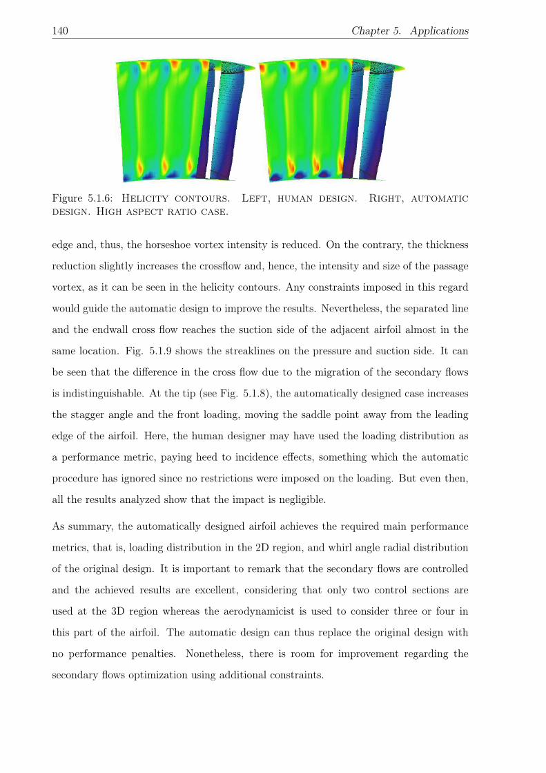
140 Chapter 5. Applications
Figure 5.1.6: Helicity contours. Left, human design. Right, automaticdesign. High aspect ratio case.
edge and, thus, the horseshoe vortex intensity is reduced. On the contrary, the thickness
reduction slightly increases the crossflow and, hence, the intensity and size of the passage
vortex, as it can be seen in the helicity contours. Any constraints imposed in this regard
would guide the automatic design to improve the results. Nevertheless, the separated line
and the endwall cross flow reaches the suction side of the adjacent airfoil almost in the
same location. Fig. 5.1.9 shows the streaklines on the pressure and suction side. It can
be seen that the difference in the cross flow due to the migration of the secondary flows
is indistinguishable. At the tip (see Fig. 5.1.8), the automatically designed case increases
the stagger angle and the front loading, moving the saddle point away from the leading
edge of the airfoil. Here, the human designer may have used the loading distribution as
a performance metric, paying heed to incidence effects, something which the automatic
procedure has ignored since no restrictions were imposed on the loading. But even then,
all the results analyzed show that the impact is negligible.
As summary, the automatically designed airfoil achieves the required main performance
metrics, that is, loading distribution in the 2D region, and whirl angle radial distribution
of the original design. It is important to remark that the secondary flows are controlled
and the achieved results are excellent, considering that only two control sections are
used at the 3D region whereas the aerodynamicist is used to consider three or four in
this part of the airfoil. The automatic design can thus replace the original design with
no performance penalties. Nonetheless, there is room for improvement regarding the
secondary flows optimization using additional constraints.
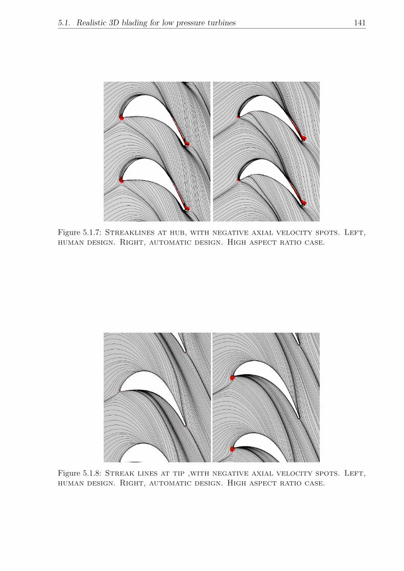
5.1. Realistic 3D blading for low pressure turbines 141
Figure 5.1.7: Streaklines at hub, with negative axial velocity spots. Left,human design. Right, automatic design. High aspect ratio case.
Figure 5.1.8: Streak lines at tip ,with negative axial velocity spots. Left,human design. Right, automatic design. High aspect ratio case.
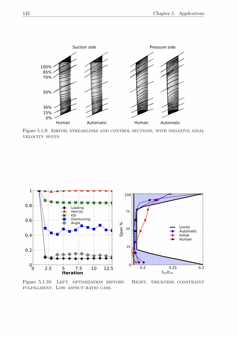
142 Chapter 5. Applications
Human Automatic
Suction side Pressure side
Human Automatic
100%85%70%
50%
30%15%
0%
Figure 5.1.9: Airfoil streaklines and control sections, with negative axialvelocity spots.
LoadingHelicityKSIOverturningAngle
0
0.2
0.4
0.6
0.8
1
Iteration0 2.5 5 7.5 10 12.5
Span%
0
100
tmx/cax0.2 0.25 0.3
50
75
25
LimitsAutomaticInitialHuman
Figure 5.1.10: Left, optimization history. Right, thickness constraintfulfillment. Low aspect ratio case.
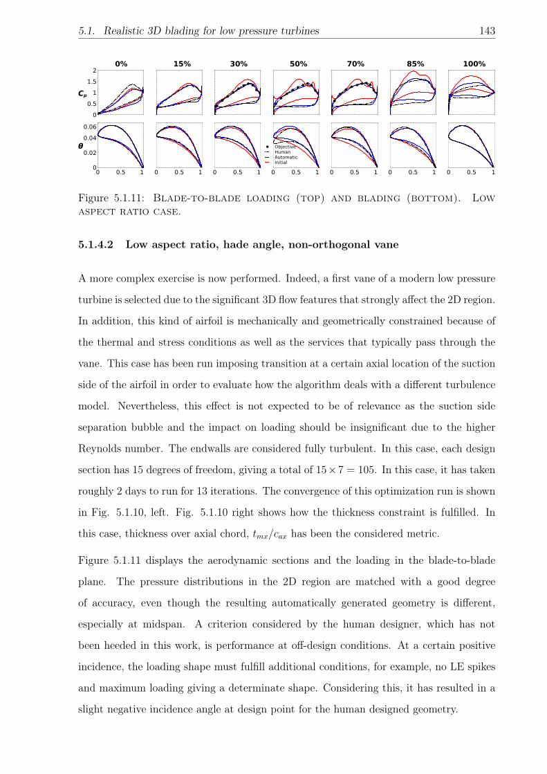
5.1. Realistic 3D blading for low pressure turbines 143
0%
Cp
0
0.5
1
1.5
215% 30%
ObjectiveHumanAutomaticInitial
50% 70% 85% 100%
θ
0
0.02
0.04
0.06
0 0.5 1 0 0.5 1 0 0.5 1 0 0.5 1 0 0.5 1 0 0.5 1 0 0.5 1
Figure 5.1.11: Blade-to-blade loading (top) and blading (bottom). Lowaspect ratio case.
5.1.4.2 Low aspect ratio, hade angle, non-orthogonal vane
A more complex exercise is now performed. Indeed, a first vane of a modern low pressure
turbine is selected due to the significant 3D flow features that strongly affect the 2D region.
In addition, this kind of airfoil is mechanically and geometrically constrained because of
the thermal and stress conditions as well as the services that typically pass through the
vane. This case has been run imposing transition at a certain axial location of the suction
side of the airfoil in order to evaluate how the algorithm deals with a different turbulence
model. Nevertheless, this effect is not expected to be of relevance as the suction side
separation bubble and the impact on loading should be insignificant due to the higher
Reynolds number. The endwalls are considered fully turbulent. In this case, each design
section has 15 degrees of freedom, giving a total of 15×7 = 105. In this case, it has taken
roughly 2 days to run for 13 iterations. The convergence of this optimization run is shown
in Fig. 5.1.10, left. Fig. 5.1.10 right shows how the thickness constraint is fulfilled. In
this case, thickness over axial chord, tmx/cax has been the considered metric.
Figure 5.1.11 displays the aerodynamic sections and the loading in the blade-to-blade
plane. The pressure distributions in the 2D region are matched with a good degree
of accuracy, even though the resulting automatically generated geometry is different,
especially at midspan. A criterion considered by the human designer, which has not
been heeded in this work, is performance at off-design conditions. At a certain positive
incidence, the loading shape must fulfill additional conditions, for example, no LE spikes
and maximum loading giving a determinate shape. Considering this, it has resulted in a
slight negative incidence angle at design point for the human designed geometry.
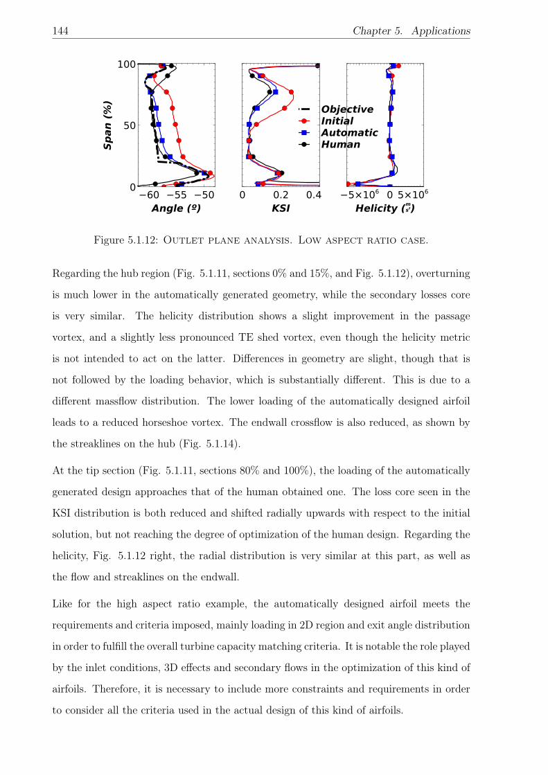
144 Chapter 5. Applications
ObjectiveInitialAutomaticHumanS
pan(%
)
0
50
100
Angle (º)−60 −55 −50
KSI0 0.2 0.4
Helicity (s2m)
−5×10⁶ 0 5×10⁶
Figure 5.1.12: Outlet plane analysis. Low aspect ratio case.
Regarding the hub region (Fig. 5.1.11, sections 0% and 15%, and Fig. 5.1.12), overturning
is much lower in the automatically generated geometry, while the secondary losses core
is very similar. The helicity distribution shows a slight improvement in the passage
vortex, and a slightly less pronounced TE shed vortex, even though the helicity metric
is not intended to act on the latter. Differences in geometry are slight, though that is
not followed by the loading behavior, which is substantially different. This is due to a
different massflow distribution. The lower loading of the automatically designed airfoil
leads to a reduced horseshoe vortex. The endwall crossflow is also reduced, as shown by
the streaklines on the hub (Fig. 5.1.14).
At the tip section (Fig. 5.1.11, sections 80% and 100%), the loading of the automatically
generated design approaches that of the human obtained one. The loss core seen in the
KSI distribution is both reduced and shifted radially upwards with respect to the initial
solution, but not reaching the degree of optimization of the human design. Regarding the
helicity, Fig. 5.1.12 right, the radial distribution is very similar at this part, as well as
the flow and streaklines on the endwall.
Like for the high aspect ratio example, the automatically designed airfoil meets the
requirements and criteria imposed, mainly loading in 2D region and exit angle distribution
in order to fulfill the overall turbine capacity matching criteria. It is notable the role played
by the inlet conditions, 3D effects and secondary flows in the optimization of this kind of
airfoils. Therefore, it is necessary to include more constraints and requirements in order
to consider all the criteria used in the actual design of this kind of airfoils.
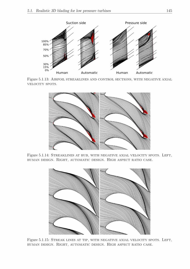
5.1. Realistic 3D blading for low pressure turbines 145
Human Automatic
Suction side Pressure side
Human Automatic
100%85%
70%
50%
30%15%
0%
Figure 5.1.13: Airfoil streaklines and control sections, with negative axialvelocity spots.
Figure 5.1.14: Streaklines at hub, with negative axial velocity spots. Left,human design. Right, automatic design. High aspect ratio case.
Figure 5.1.15: Streak lines at tip, with negative axial velocity spots. Left,human design. Right, automatic design. High aspect ratio case.
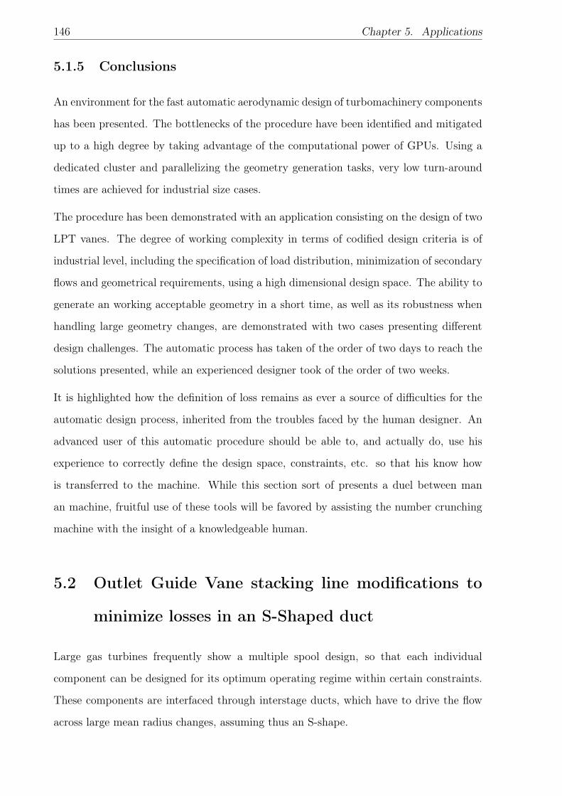
146 Chapter 5. Applications
5.1.5 Conclusions
An environment for the fast automatic aerodynamic design of turbomachinery components
has been presented. The bottlenecks of the procedure have been identified and mitigated
up to a high degree by taking advantage of the computational power of GPUs. Using a
dedicated cluster and parallelizing the geometry generation tasks, very low turn-around
times are achieved for industrial size cases.
The procedure has been demonstrated with an application consisting on the design of two
LPT vanes. The degree of working complexity in terms of codified design criteria is of
industrial level, including the specification of load distribution, minimization of secondary
flows and geometrical requirements, using a high dimensional design space. The ability to
generate an working acceptable geometry in a short time, as well as its robustness when
handling large geometry changes, are demonstrated with two cases presenting different
design challenges. The automatic process has taken of the order of two days to reach the
solutions presented, while an experienced designer took of the order of two weeks.
It is highlighted how the definition of loss remains as ever a source of difficulties for the
automatic design process, inherited from the troubles faced by the human designer. An
advanced user of this automatic procedure should be able to, and actually do, use his
experience to correctly define the design space, constraints, etc. so that his know how
is transferred to the machine. While this section sort of presents a duel between man
an machine, fruitful use of these tools will be favored by assisting the number crunching
machine with the insight of a knowledgeable human.
5.2 Outlet Guide Vane stacking line modifications to
minimize losses in an S-Shaped duct
Large gas turbines frequently show a multiple spool design, so that each individual
component can be designed for its optimum operating regime within certain constraints.
These components are interfaced through interstage ducts, which have to drive the flow
across large mean radius changes, assuming thus an S-shape.
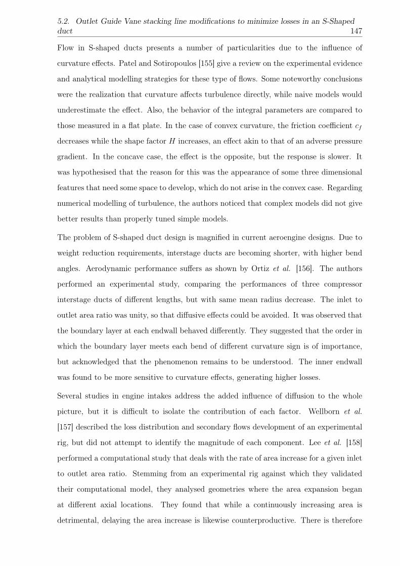
5.2. Outlet Guide Vane stacking line modifications to minimize losses in an S-Shapedduct 147
Flow in S-shaped ducts presents a number of particularities due to the influence of
curvature effects. Patel and Sotiropoulos [155] give a review on the experimental evidence
and analytical modelling strategies for these type of flows. Some noteworthy conclusions
were the realization that curvature affects turbulence directly, while naive models would
underestimate the effect. Also, the behavior of the integral parameters are compared to
those measured in a flat plate. In the case of convex curvature, the friction coefficient cf
decreases while the shape factor H increases, an effect akin to that of an adverse pressure
gradient. In the concave case, the effect is the opposite, but the response is slower. It
was hypothesised that the reason for this was the appearance of some three dimensional
features that need some space to develop, which do not arise in the convex case. Regarding
numerical modelling of turbulence, the authors noticed that complex models did not give
better results than properly tuned simple models.
The problem of S-shaped duct design is magnified in current aeroengine designs. Due to
weight reduction requirements, interstage ducts are becoming shorter, with higher bend
angles. Aerodynamic performance suffers as shown by Ortiz et al. [156]. The authors
performed an experimental study, comparing the performances of three compressor
interstage ducts of different lengths, but with same mean radius decrease. The inlet to
outlet area ratio was unity, so that diffusive effects could be avoided. It was observed that
the boundary layer at each endwall behaved differently. They suggested that the order in
which the boundary layer meets each bend of different curvature sign is of importance,
but acknowledged that the phenomenon remains to be understood. The inner endwall
was found to be more sensitive to curvature effects, generating higher losses.
Several studies in engine intakes address the added influence of diffusion to the whole
picture, but it is difficult to isolate the contribution of each factor. Wellborn et al.
[157] described the loss distribution and secondary flows development of an experimental
rig, but did not attempt to identify the magnitude of each component. Lee et al. [158]
performed a computational study that deals with the rate of area increase for a given inlet
to outlet area ratio. Stemming from an experimental rig against which they validated
their computational model, they analysed geometries where the area expansion began
at different axial locations. They found that while a continuously increasing area is
detrimental, delaying the area increase is likewise counterproductive. There is therefore
148 Chapter 5. Applications
an optimum to be found.
It was mentioned earlier that curvature has a pressure gradient-like effect. Therefore, some
conclusions drawn from constant radius diffusers may be applicable. Zierer [159] tested
a straight annular diffuser at several inlet conditions, representing different operating
points. He concluded that radial velocity distribution and the state of the inlet boundary
layer played a crucial role in pressure recovery.
Compared to other aerospace applications, engine ducts present an additional complica-
tion in the shape of the interaction between the secondary flows induced by the airfoil
rows and those originated within the duct itself. Furthermore, the nearer the airfoil to the
duct, the less developed these features are, and the more difficult they are to predict. An
integrated design would be an airfoil row placed within the duct. Walker et al. [160] pro-
posed a design methodology to achieve an integrated design with the same performance as
a longer non integrated one, where flow features are easier to predict. Applying a straight
tangential lean to the airfoils, they managed to matched the outlet static pressure field
and total losses in both configurations. However, they did not describe the meridional
flow field, so the mechanisms they exploited cannot be ascertained.
In this study, the idea suggested by Walker et al. is pursued further. Complex tangential
lean is applied to an integrated airfoil-duct design with the aim of minimizing aerodynamic
losses. The mechanisms by which improvements are achieved are described in detail.
5.2.1 Problem description and set up
5.2.1.1 Base geometry and design space
The problem at hand is the interstage duct between the low pressure and the high pressure
compressor modules, seen in figure 5.2.1. It is a short duct with aggressive bends, with
two integrated airfoil rows. The first one is the last stator stage, whose purpose is swirl
recovery before entering the following module. The other is a row of structural vanes,
with no aerodynamic function. There is no possibility of modifying the geometry of the
duct or the structural vanes, so it can only be acted on the stator.
Thus, the computational domain comprises a duct section between two normal planes.
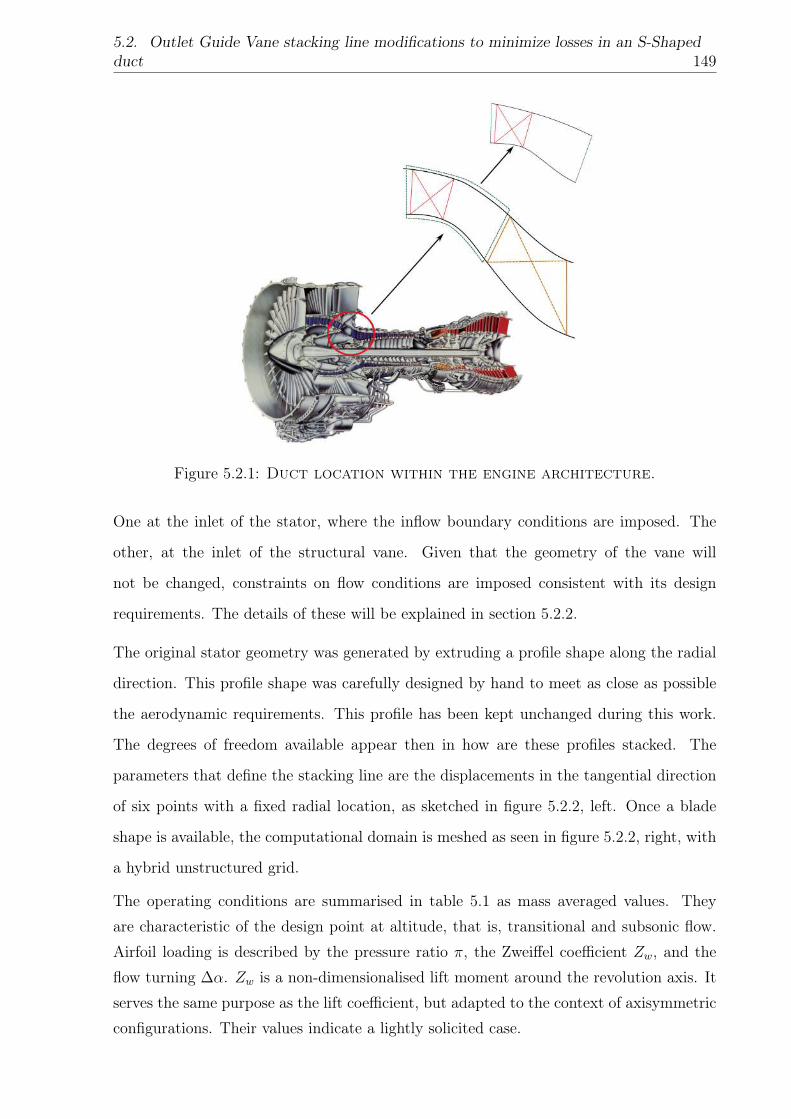
5.2. Outlet Guide Vane stacking line modifications to minimize losses in an S-Shapedduct 149
Figure 5.2.1: Duct location within the engine architecture.
One at the inlet of the stator, where the inflow boundary conditions are imposed. The
other, at the inlet of the structural vane. Given that the geometry of the vane will
not be changed, constraints on flow conditions are imposed consistent with its design
requirements. The details of these will be explained in section 5.2.2.
The original stator geometry was generated by extruding a profile shape along the radial
direction. This profile shape was carefully designed by hand to meet as close as possible
the aerodynamic requirements. This profile has been kept unchanged during this work.
The degrees of freedom available appear then in how are these profiles stacked. The
parameters that define the stacking line are the displacements in the tangential direction
of six points with a fixed radial location, as sketched in figure 5.2.2, left. Once a blade
shape is available, the computational domain is meshed as seen in figure 5.2.2, right, with
a hybrid unstructured grid.
The operating conditions are summarised in table 5.1 as mass averaged values. They
are characteristic of the design point at altitude, that is, transitional and subsonic flow.
Airfoil loading is described by the pressure ratio π, the Zweiffel coefficient Zw, and the
flow turning ∆α. Zw is a non-dimensionalised lift moment around the revolution axis. It
serves the same purpose as the lift coefficient, but adapted to the context of axisymmetric
configurations. Their values indicate a lightly solicited case.
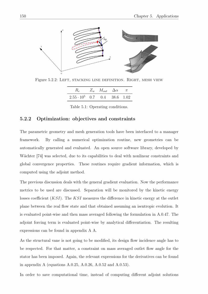
150 Chapter 5. Applications
Figure 5.2.2: Left, stacking line definition. Right, mesh view
Re Zw Mout ∆α π
2.55 · 105 0.7 0.4 38.6 1.02
Table 5.1: Operating conditions.
5.2.2 Optimization: objectives and constraints
The parametric geometry and mesh generation tools have been interfaced to a manager
framework. By calling a numerical optimization routine, new geometries can be
automatically generated and evaluated. An open source software library, developed by
Wächter [74] was selected, due to its capabilities to deal with nonlinear constraints and
global convergence properties. These routines require gradient information, which is
computed using the adjoint method.
The previous discussion deals with the general gradient evaluation. Now the performance
metrics to be used are discussed. Separation will be monitored by the kinetic energy
losses coefficient (KSI). The KSI measures the difference in kinetic energy at the outlet
plane between the real flow state and that obtained assuming an isentropic evolution. It
is evaluated point-wise and then mass averaged following the formulation in A.0.47. The
adjoint forcing term is evaluated point-wise by analytical differentiation. The resulting
expressions can be found in appendix A A.
As the structural vane is not going to be modified, its design flow incidence angle has to
be respected. For that matter, a constraint on mass averaged outlet flow angle for the
stator has been imposed. Again, the relevant expressions for the derivatives can be found
in appendix A (equations A.0.25, A.0.26, A.0.52 and A.0.53).
In order to save computational time, instead of computing different adjoint solutions
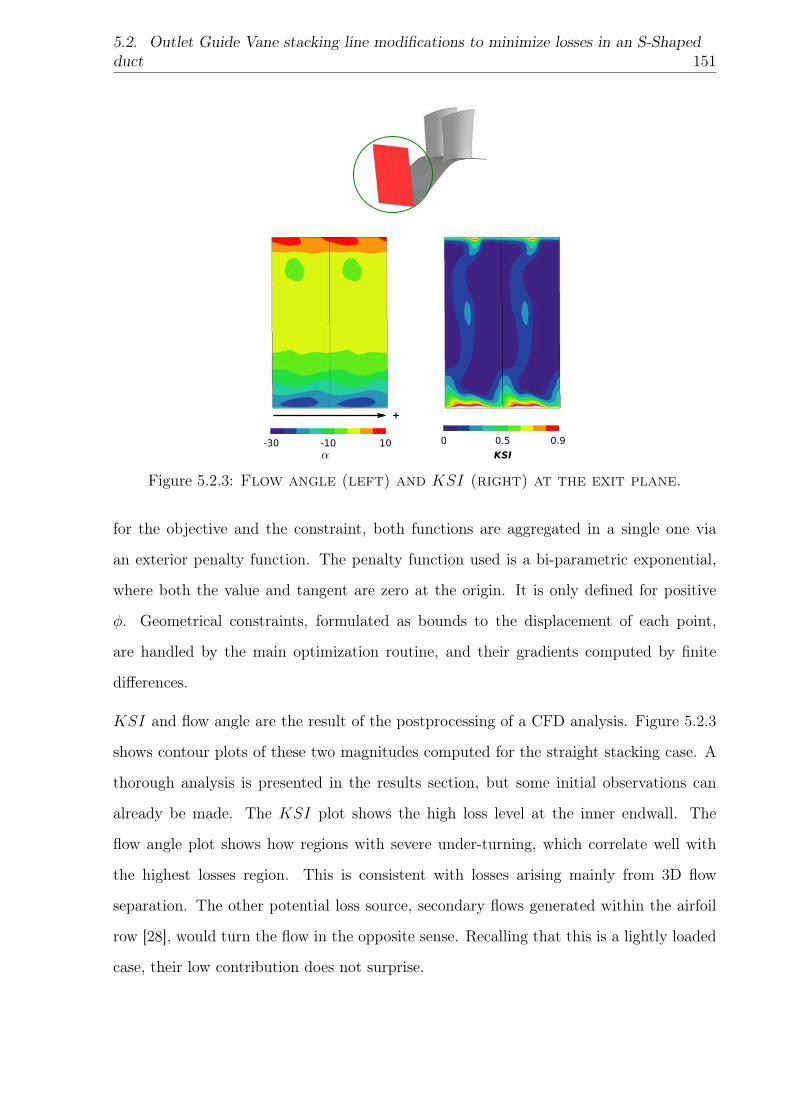
5.2. Outlet Guide Vane stacking line modifications to minimize losses in an S-Shapedduct 151
Figure 5.2.3: Flow angle (left) and KSI (right) at the exit plane.
for the objective and the constraint, both functions are aggregated in a single one via
an exterior penalty function. The penalty function used is a bi-parametric exponential,
where both the value and tangent are zero at the origin. It is only defined for positive
φ. Geometrical constraints, formulated as bounds to the displacement of each point,
are handled by the main optimization routine, and their gradients computed by finite
differences.
KSI and flow angle are the result of the postprocessing of a CFD analysis. Figure 5.2.3
shows contour plots of these two magnitudes computed for the straight stacking case. A
thorough analysis is presented in the results section, but some initial observations can
already be made. The KSI plot shows the high loss level at the inner endwall. The
flow angle plot shows how regions with severe under-turning, which correlate well with
the highest losses region. This is consistent with losses arising mainly from 3D flow
separation. The other potential loss source, secondary flows generated within the airfoil
row [28], would turn the flow in the opposite sense. Recalling that this is a lightly loaded
case, their low contribution does not surprise.
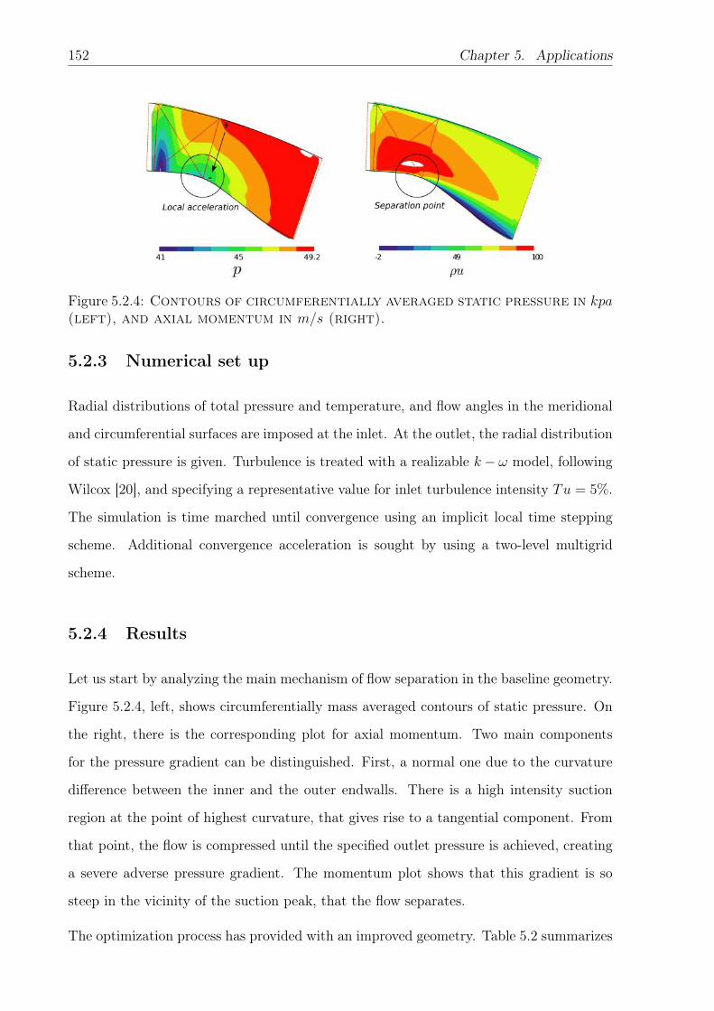
152 Chapter 5. Applications
Figure 5.2.4: Contours of circumferentially averaged static pressure in kpa(left), and axial momentum in m/s (right).
5.2.3 Numerical set up
Radial distributions of total pressure and temperature, and flow angles in the meridional
and circumferential surfaces are imposed at the inlet. At the outlet, the radial distribution
of static pressure is given. Turbulence is treated with a realizable k − ω model, following
Wilcox [20], and specifying a representative value for inlet turbulence intensity Tu = 5%.
The simulation is time marched until convergence using an implicit local time stepping
scheme. Additional convergence acceleration is sought by using a two-level multigrid
scheme.
5.2.4 Results
Let us start by analyzing the main mechanism of flow separation in the baseline geometry.
Figure 5.2.4, left, shows circumferentially mass averaged contours of static pressure. On
the right, there is the corresponding plot for axial momentum. Two main components
for the pressure gradient can be distinguished. First, a normal one due to the curvature
difference between the inner and the outer endwalls. There is a high intensity suction
region at the point of highest curvature, that gives rise to a tangential component. From
that point, the flow is compressed until the specified outlet pressure is achieved, creating
a severe adverse pressure gradient. The momentum plot shows that this gradient is so
steep in the vicinity of the suction peak, that the flow separates.
The optimization process has provided with an improved geometry. Table 5.2 summarizes
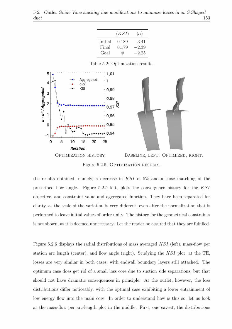
5.2. Outlet Guide Vane stacking line modifications to minimize losses in an S-Shapedduct 153
〈KSI〉 〈α〉
Initial 0.189 −3.41Final 0.179 −2.39Goal ∅ −2.25
Table 5.2: Optimization results.
Aggregated
α-α*
KSI
KSI
0,94
0,95
0,96
0,97
0,98
0,99
1
1,01
α - α* / Aggregated
−1
0
1
2
3
4
5
Iteration
0 5 10 15 20 25
Optimization history Baseline, left. Optimized, right.
Figure 5.2.5: Optimization results.
the results obtained, namely, a decrease in KSI of 5% and a close matching of the
prescribed flow angle. Figure 5.2.5 left, plots the convergence history for the KSI
objective, and constraint value and aggregated function. They have been separated for
clarity, as the scale of the variation is very different, even after the normalization that is
performed to leave initial values of order unity. The history for the geometrical constraints
is not shown, as it is deemed unnecessary. Let the reader be assured that they are fulfilled.
Figure 5.2.6 displays the radial distributions of mass averaged KSI (left), mass-flow per
station arc length (center), and flow angle (right). Studying the KSI plot, at the TE,
losses are very similar in both cases, with endwall boundary layers still attached. The
optimum case does get rid of a small loss core due to suction side separations, but that
should not have dramatic consequences in principle. At the outlet, however, the loss
distributions differ noticeably, with the optimal case exhibiting a lower entrainment of
low energy flow into the main core. In order to understand how is this so, let us look
at the mass-flow per arc-length plot in the middle. First, one caveat, the distributions
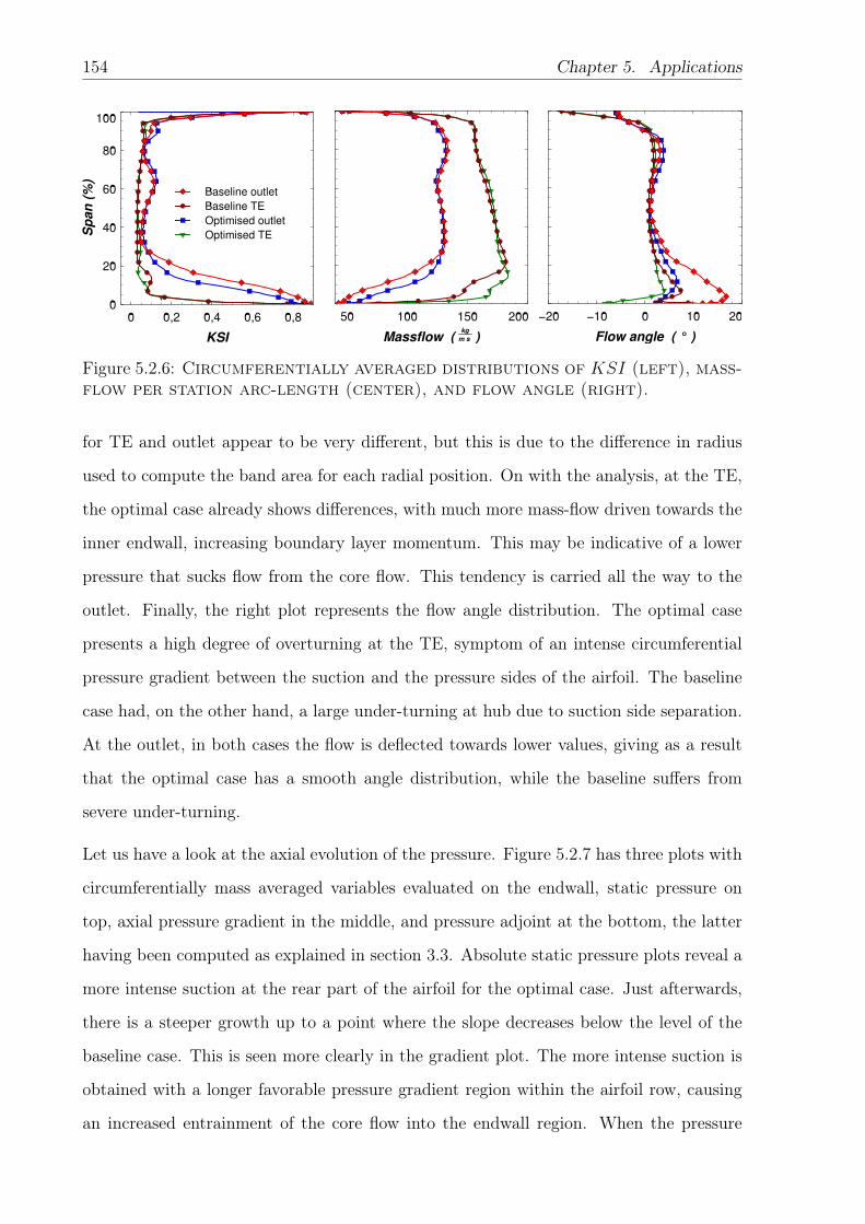
154 Chapter 5. Applications
Figure 5.2.6: Circumferentially averaged distributions of KSI (left), mass-flow per station arc-length (center), and flow angle (right).
for TE and outlet appear to be very different, but this is due to the difference in radius
used to compute the band area for each radial position. On with the analysis, at the TE,
the optimal case already shows differences, with much more mass-flow driven towards the
inner endwall, increasing boundary layer momentum. This may be indicative of a lower
pressure that sucks flow from the core flow. This tendency is carried all the way to the
outlet. Finally, the right plot represents the flow angle distribution. The optimal case
presents a high degree of overturning at the TE, symptom of an intense circumferential
pressure gradient between the suction and the pressure sides of the airfoil. The baseline
case had, on the other hand, a large under-turning at hub due to suction side separation.
At the outlet, in both cases the flow is deflected towards lower values, giving as a result
that the optimal case has a smooth angle distribution, while the baseline suffers from
severe under-turning.
Let us have a look at the axial evolution of the pressure. Figure 5.2.7 has three plots with
circumferentially mass averaged variables evaluated on the endwall, static pressure on
top, axial pressure gradient in the middle, and pressure adjoint at the bottom, the latter
having been computed as explained in section 3.3. Absolute static pressure plots reveal a
more intense suction at the rear part of the airfoil for the optimal case. Just afterwards,
there is a steeper growth up to a point where the slope decreases below the level of the
baseline case. This is seen more clearly in the gradient plot. The more intense suction is
obtained with a longer favorable pressure gradient region within the airfoil row, causing
an increased entrainment of the core flow into the endwall region. When the pressure
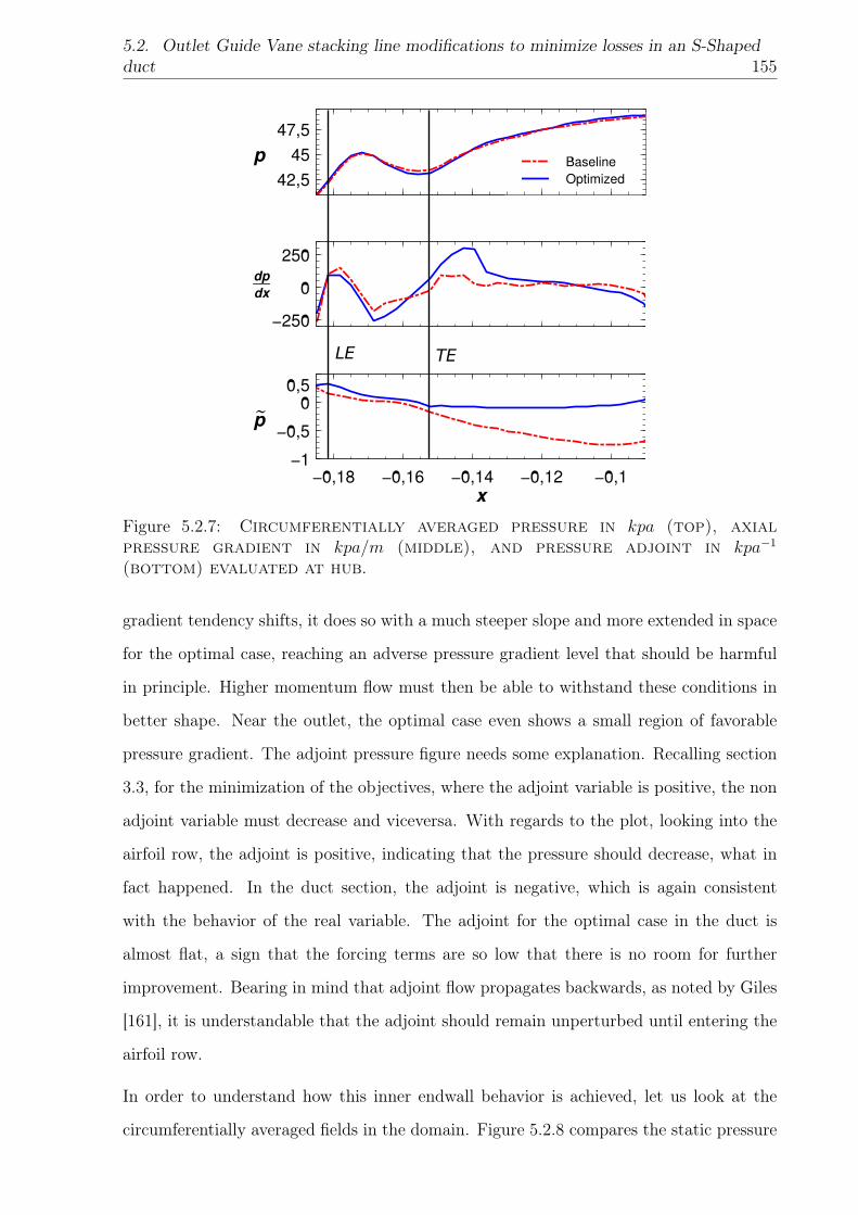
5.2. Outlet Guide Vane stacking line modifications to minimize losses in an S-Shapedduct 155
Figure 5.2.7: Circumferentially averaged pressure in kpa (top), axialpressure gradient in kpa/m (middle), and pressure adjoint in kpa−1
(bottom) evaluated at hub.
gradient tendency shifts, it does so with a much steeper slope and more extended in space
for the optimal case, reaching an adverse pressure gradient level that should be harmful
in principle. Higher momentum flow must then be able to withstand these conditions in
better shape. Near the outlet, the optimal case even shows a small region of favorable
pressure gradient. The adjoint pressure figure needs some explanation. Recalling section
3.3, for the minimization of the objectives, where the adjoint variable is positive, the non
adjoint variable must decrease and viceversa. With regards to the plot, looking into the
airfoil row, the adjoint is positive, indicating that the pressure should decrease, what in
fact happened. In the duct section, the adjoint is negative, which is again consistent
with the behavior of the real variable. The adjoint for the optimal case in the duct is
almost flat, a sign that the forcing terms are so low that there is no room for further
improvement. Bearing in mind that adjoint flow propagates backwards, as noted by Giles
[161], it is understandable that the adjoint should remain unperturbed until entering the
airfoil row.
In order to understand how this inner endwall behavior is achieved, let us look at the
circumferentially averaged fields in the domain. Figure 5.2.8 compares the static pressure
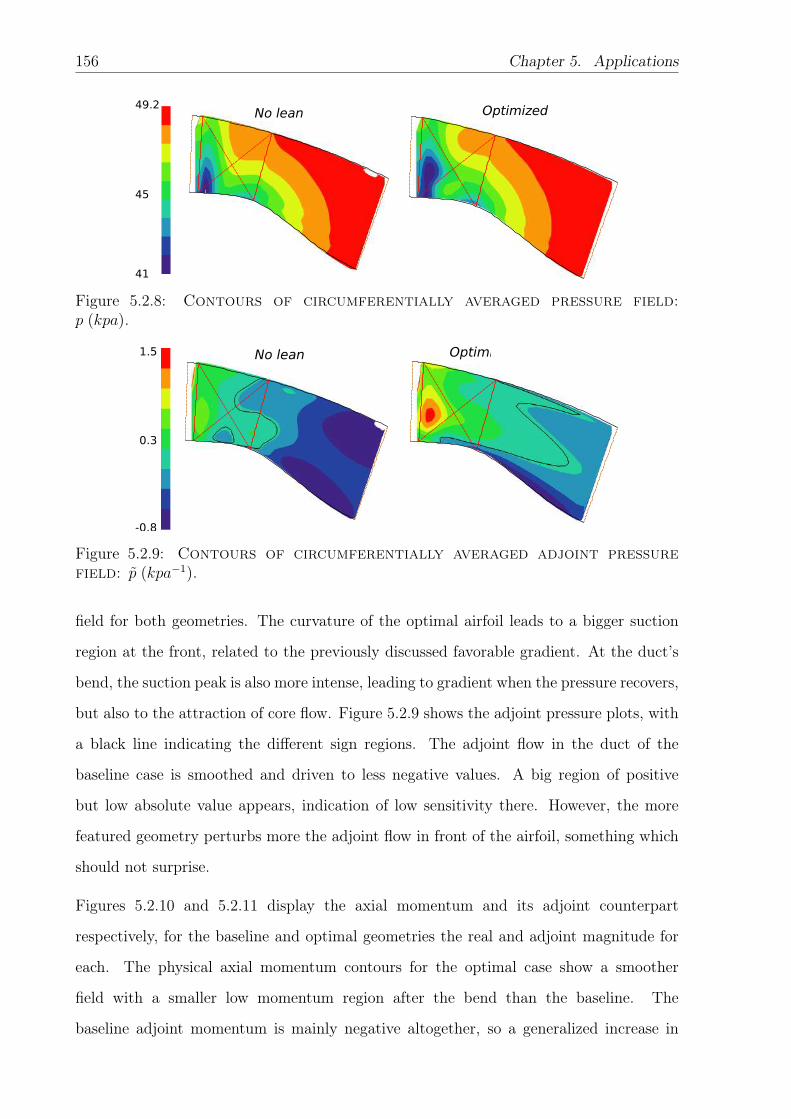
156 Chapter 5. Applications
Figure 5.2.8: Contours of circumferentially averaged pressure field:p (kpa).
Figure 5.2.9: Contours of circumferentially averaged adjoint pressurefield: p (kpa−1).
field for both geometries. The curvature of the optimal airfoil leads to a bigger suction
region at the front, related to the previously discussed favorable gradient. At the duct’s
bend, the suction peak is also more intense, leading to gradient when the pressure recovers,
but also to the attraction of core flow. Figure 5.2.9 shows the adjoint pressure plots, with
a black line indicating the different sign regions. The adjoint flow in the duct of the
baseline case is smoothed and driven to less negative values. A big region of positive
but low absolute value appears, indication of low sensitivity there. However, the more
featured geometry perturbs more the adjoint flow in front of the airfoil, something which
should not surprise.
Figures 5.2.10 and 5.2.11 display the axial momentum and its adjoint counterpart
respectively, for the baseline and optimal geometries the real and adjoint magnitude for
each. The physical axial momentum contours for the optimal case show a smoother
field with a smaller low momentum region after the bend than the baseline. The
baseline adjoint momentum is mainly negative altogether, so a generalized increase in
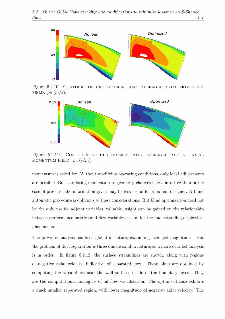
5.2. Outlet Guide Vane stacking line modifications to minimize losses in an S-Shapedduct 157
Figure 5.2.10: Contours of circumferentially averaged axial momentumfield: ρu (m/s).
Figure 5.2.11: Contours of circumferentially averaged adjoint axialmomentum field: ρu (s/m).
momentum is asked for. Without modifying operating conditions, only local adjustments
are possible. But as relating momentum to geometry changes is less intuitive than in the
case of pressure, the information given may be less useful for a human designer. A blind
automatic procedure is oblivious to these considerations. But blind optimization need not
be the only use for adjoint variables, valuable insight can be gained on the relationship
between performance metrics and flow variables, useful for the understanding of physical
phenomena.
The previous analysis has been global in nature, examining averaged magnitudes. But
the problem of duct separation is three dimensional in nature, so a more detailed analysis
is in order. In figure 5.2.12, the surface streamlines are shown, along with regions
of negative axial velocity, indicative of separated flow. These plots are obtained by
computing the streamlines near the wall surface, inside of the boundary layer. They
are the computational analogues of oil flow visualization. The optimized case exhibits
a much smaller separated region, with lower magnitude of negative axial velocity. The
158 Chapter 5. Applications
separation at the pressure side of the airfoil is also, smaller, which explains the smaller
loss core from the KSI distribution evaluated at the TE. The separated region is confined
within a region bounded by dividing streamlines and more loosely by critical points.
In figure 5.2.14, the streamlines are plotted against a contour of velocity divergence,
which is the trace of the velocity deformation tensor. According to phase plane theory,
the nature of critical points is related to the trace and determinant of the matrix of the
dynamical system. Figure 5.2.13 shows that the trace determines the stability properties,
and the determinant the qualitative behavior. From the streamlines, the type of point is
immediately discernible. The divergence adds the stability information. Gbadebo et al.
[162] provide with a description of 3D flow separation in axial compressors. They noted
that the number and type of critical points is constrained by topological relations, i. e.,
the numbers of saddle points and nodes is related by an index rule. They provide with
this rule, which is applicable to a generic airfoil row. A corollary is that, counting the
numbers of nodes, the number of saddle points to look for is known, and viceversa.
Both geometries exhibit the same topology, meaning that passive separation control is
achieved not with dramatic flow feature changes, but with subtle perturbations. There
is a stable focus at the suction side near the inner endwall in both cases, marking
the separation point over there. Separated flow then leaves a track at the endwall
distinguishable by the visible dividing streamlines. The wake divides this separated region
in two sides, where a saddle point signals another separation in the shape of counter
rotating vortexes. This is deduced as in a saddle, one critical line marks separation,
and the other reattachment. In this case, the transverse one is a lift-off line, the axial
separates the counter-rotating vortexes which rotate so that the down-wash forms that
line. Downstream of this saddle, some of the flow in these vortexes reattaches in two
unstable focii. In the baseline case, these are very close, and their interaction leads to
another lift-off just downstream. In the optimized case, they are more spread, and a
channel of fully attached flow exists. Near the outlet, for the baseline case, the flow
reattaches across the whole span of the channel, a feature signaled by an agglomeration
of streamlines, some of them coming from the attachment line of a rear saddle. In the
optimal case, the flow behaves similarly, but there is no streamline concentration.
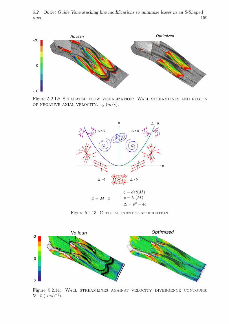
5.2. Outlet Guide Vane stacking line modifications to minimize losses in an S-Shapedduct 159
Figure 5.2.12: Separated flow visualization: Wall streamlines and regionof negative axial velocity: vx (m/s).
Figure 5.2.13: Critical point classification.
Figure 5.2.14: Wall streamlines against velocity divergence contours:∇ · v ((ms)−1).
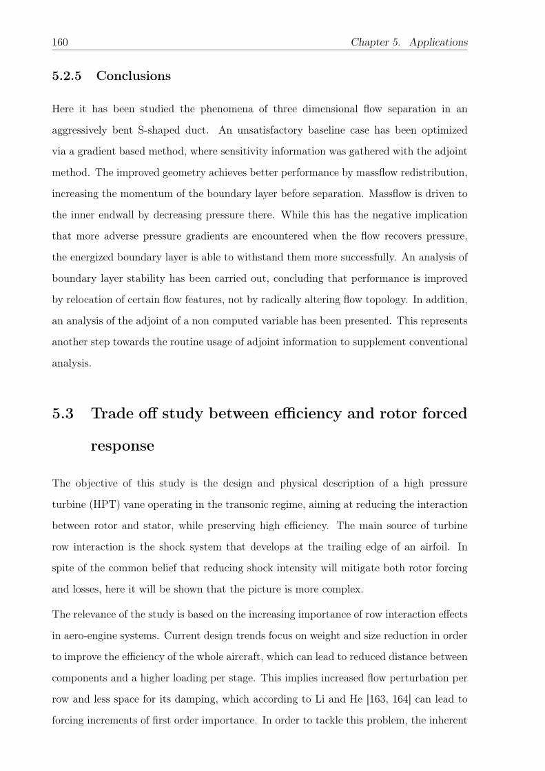
160 Chapter 5. Applications
5.2.5 Conclusions
Here it has been studied the phenomena of three dimensional flow separation in an
aggressively bent S-shaped duct. An unsatisfactory baseline case has been optimized
via a gradient based method, where sensitivity information was gathered with the adjoint
method. The improved geometry achieves better performance by massflow redistribution,
increasing the momentum of the boundary layer before separation. Massflow is driven to
the inner endwall by decreasing pressure there. While this has the negative implication
that more adverse pressure gradients are encountered when the flow recovers pressure,
the energized boundary layer is able to withstand them more successfully. An analysis of
boundary layer stability has been carried out, concluding that performance is improved
by relocation of certain flow features, not by radically altering flow topology. In addition,
an analysis of the adjoint of a non computed variable has been presented. This represents
another step towards the routine usage of adjoint information to supplement conventional
analysis.
5.3 Trade off study between efficiency and rotor forced
response
The objective of this study is the design and physical description of a high pressure
turbine (HPT) vane operating in the transonic regime, aiming at reducing the interaction
between rotor and stator, while preserving high efficiency. The main source of turbine
row interaction is the shock system that develops at the trailing edge of an airfoil. In
spite of the common belief that reducing shock intensity will mitigate both rotor forcing
and losses, here it will be shown that the picture is more complex.
The relevance of the study is based on the increasing importance of row interaction effects
in aero-engine systems. Current design trends focus on weight and size reduction in order
to improve the efficiency of the whole aircraft, which can lead to reduced distance between
components and a higher loading per stage. This implies increased flow perturbation per
row and less space for its damping, which according to Li and He [163, 164] can lead to
forcing increments of first order importance. In order to tackle this problem, the inherent

5.3. Trade off study between efficiency and rotor forced response 161
unsteadiness of the flow field should be taken into consideration in every stage of the
design process.
Several sources of flow unsteadiness have been identified, with comprehensive accounts
found in Paniagua [165] and Payne [166]. These can be classified as pressure waves
propagation or potential effects, viscous effects where convection of low momentum flow
causes local pressure distortions, and shock waves. Supersonic flow is characterized by
the limited attenuation of propagated perturbations. Therefore, the interaction between
blade rows in transonic turbine stages will be of higher importance than in subsonic stages.
Barter et al. [167] investigated numerically the propagation of shocks across a stage,
both considering and neglecting wave reflections between rows. Results showed that the
stator’s trailing edge shocks, when reflected from the rotor, do have an important impact
on the vane’s loading, but successive reflections back to the rotor pose an influence of
second order. Barter argued that only the unsteady frequency component corresponding
to the first harmonic of the excitation is relevant. However, Kammerer and Abhari [168]
demonstrated experimentally the importance of higher order harmonics.
Work on this topic has been carried out in the past at the von Karman Institute.
Vascellari et al. [169] identified numerically the particularities of 2D profile velocity
distributions that give rise to the trailing edge shock system. Joly et al. [48] set
as objective the minimization of vane outlet inhomogeneities using multi-objective
optimization techniques, revealing that efficiency and unsteady forcing are conflicting
objectives. Multiple shock reflections may result in a reduced forcing at the expense of
higher loss. They described a geometry which achieves the same efficiency as a baseline
one, while also minimizing the outlet pressure distortion. The pressure side was heavily
modified, generating a narrower channel with a divergent passage. The sonic line shifted
upstream, resulting in a larger acceleration at the pressure side, coupled with a straight
suction side rear part. This resulted in a reduction of the pressure difference at the trailing
edge.
Previous research was focused in the study of 2D profiles, an approach that is not
applicable to low aspect ratio turbomachinery flows, which are highly three-dimensional.
The novelty of the current research is the identification of various 3D flow field features
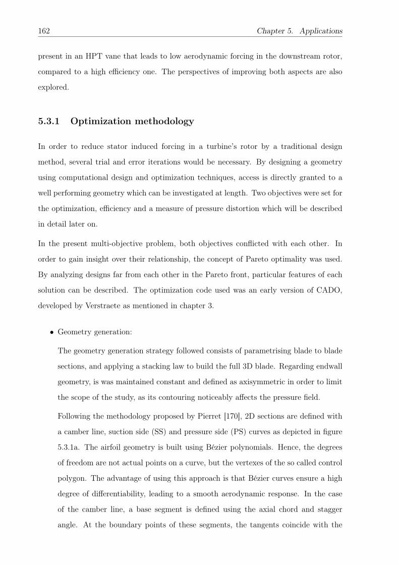
162 Chapter 5. Applications
present in an HPT vane that leads to low aerodynamic forcing in the downstream rotor,
compared to a high efficiency one. The perspectives of improving both aspects are also
explored.
5.3.1 Optimization methodology
In order to reduce stator induced forcing in a turbine’s rotor by a traditional design
method, several trial and error iterations would be necessary. By designing a geometry
using computational design and optimization techniques, access is directly granted to a
well performing geometry which can be investigated at length. Two objectives were set for
the optimization, efficiency and a measure of pressure distortion which will be described
in detail later on.
In the present multi-objective problem, both objectives conflicted with each other. In
order to gain insight over their relationship, the concept of Pareto optimality was used.
By analyzing designs far from each other in the Pareto front, particular features of each
solution can be described. The optimization code used was an early version of CADO,
developed by Verstraete as mentioned in chapter 3.
• Geometry generation:
The geometry generation strategy followed consists of parametrising blade to blade
sections, and applying a stacking law to build the full 3D blade. Regarding endwall
geometry, is was maintained constant and defined as axisymmetric in order to limit
the scope of the study, as its contouring noticeably affects the pressure field.
Following the methodology proposed by Pierret [170], 2D sections are defined with
a camber line, suction side (SS) and pressure side (PS) curves as depicted in figure
5.3.1a. The airfoil geometry is built using Bézier polynomials. Hence, the degrees
of freedom are not actual points on a curve, but the vertexes of the so called control
polygon. The advantage of using this approach is that Bézier curves ensure a high
degree of differentiability, leading to a smooth aerodynamic response. In the case
of the camber line, a base segment is defined using the axial chord and stagger
angle. At the boundary points of these segments, the tangents coincide with the
5.3. Trade off study between efficiency and rotor forced response 163
inlet and outlet metal angles. The camber line is then divided in pieces using a
stretching law, which differs for constructing the SS and the PS curves. The normal
distances d1, d2 and d3 from the SS stretched distribution determine the positions
of the vertex of the control polygon that defines the SS curve. Likewise, the normal
distances d4 and d5 define the PS curve. These curves are joined at the leading
edge (LE) with second order continuity through placing the second control point of
the SS and PS curves perpendicular to the camber line at the LE, guaranteeing the
same LE curvature by constraining the relationship between these distances. This
LE curvature radius is as well a design parameter. At the trailing edge (TE), the
tangents on the SS and PS (δSS and δPS) are additional design parameters, which
set the wedge angles to close the airfoil with a TE circumference, whose radius is
imposed by manufacturing, structural, and thermal considerations.
In this work three profile sections were parametrised. In total, 10 parameters define
a profile: 4 control points for the suction side, 3 for the pressure side, the leading
edge radius, and the trailing edge’s wedge angles. The inlet metal angle was imposed
to be aligned with the inlet flow angle and the outlet metal angle was fixed at the
desired outlet flow angle. Both axial chord and stagger angles were also fixed.
The stacking line was placed at the trailing edge in order to have higher control
over the outlet flow topology. It was defined as the tangential (lean) displacement
of the TE of each section with respect to the location of the TE of the hub profile
(see figure 5.3.1b). To parametrize the lean, Bézier curves are again used. At four
equidistant radial stations (hub, tip and two other radii in between), the positions
of the Bézier control points were determined by the tip displacement, and the angles
with the radial direction at hub and tip (see figure 5.3.1c). A fixed number of airfoils
is considered, so that every geometry has the same pitch.
The three profiles and the stacking line add up to a total of 33 parameters to define
a 3D airfoil.
• Mesh generation and CFD analysis settings:
Accurate CFD loss computation posed certain requirements, both in regards to
mesh generation and flow modelling. Entropy generation mechanisms stem from
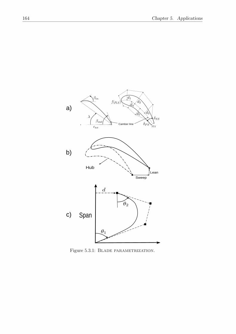
164 Chapter 5. Applications
Hub
Sweep
Lean
Span
Camber line
a)
b)
c)
Figure 5.3.1: Blade parametrization.
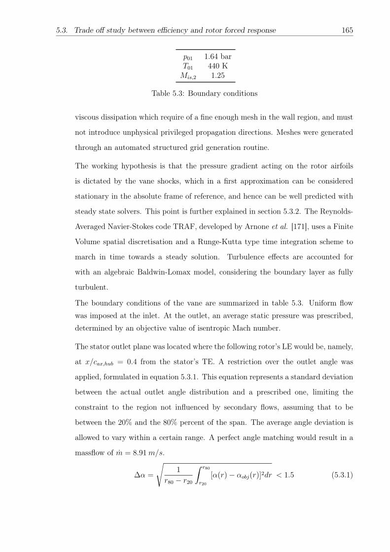
5.3. Trade off study between efficiency and rotor forced response 165
p01 1.64 barT01 440 KMis,2 1.25
Table 5.3: Boundary conditions
viscous dissipation which require of a fine enough mesh in the wall region, and must
not introduce unphysical privileged propagation directions. Meshes were generated
through an automated structured grid generation routine.
The working hypothesis is that the pressure gradient acting on the rotor airfoils
is dictated by the vane shocks, which in a first approximation can be considered
stationary in the absolute frame of reference, and hence can be well predicted with
steady state solvers. This point is further explained in section 5.3.2. The Reynolds-
Averaged Navier-Stokes code TRAF, developed by Arnone et al. [171], uses a Finite
Volume spatial discretisation and a Runge-Kutta type time integration scheme to
march in time towards a steady solution. Turbulence effects are accounted for
with an algebraic Baldwin-Lomax model, considering the boundary layer as fully
turbulent.
The boundary conditions of the vane are summarized in table 5.3. Uniform flow
was imposed at the inlet. At the outlet, an average static pressure was prescribed,
determined by an objective value of isentropic Mach number.
The stator outlet plane was located where the following rotor’s LE would be, namely,
at x/cax,hub = 0.4 from the stator’s TE. A restriction over the outlet angle was
applied, formulated in equation 5.3.1. This equation represents a standard deviation
between the actual outlet angle distribution and a prescribed one, limiting the
constraint to the region not influenced by secondary flows, assuming that to be
between the 20% and the 80% percent of the span. The average angle deviation is
allowed to vary within a certain range. A perfect angle matching would result in a
massflow of m = 8.91m/s.
∆α =
√1
r80 − r20
ˆ r80
r20
[α(r)− αobj(r)]2dr < 1.5 (5.3.1)
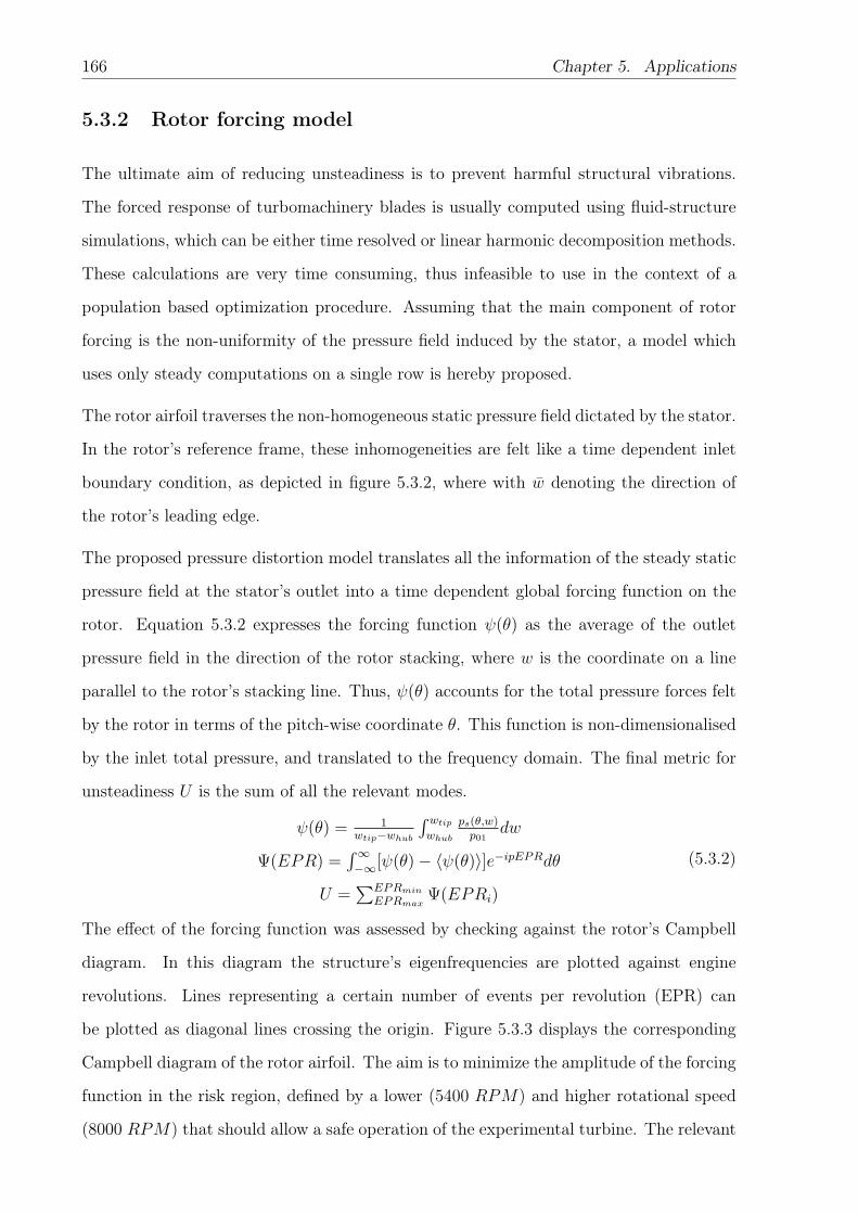
166 Chapter 5. Applications
5.3.2 Rotor forcing model
The ultimate aim of reducing unsteadiness is to prevent harmful structural vibrations.
The forced response of turbomachinery blades is usually computed using fluid-structure
simulations, which can be either time resolved or linear harmonic decomposition methods.
These calculations are very time consuming, thus infeasible to use in the context of a
population based optimization procedure. Assuming that the main component of rotor
forcing is the non-uniformity of the pressure field induced by the stator, a model which
uses only steady computations on a single row is hereby proposed.
The rotor airfoil traverses the non-homogeneous static pressure field dictated by the stator.
In the rotor’s reference frame, these inhomogeneities are felt like a time dependent inlet
boundary condition, as depicted in figure 5.3.2, where with w denoting the direction of
the rotor’s leading edge.
The proposed pressure distortion model translates all the information of the steady static
pressure field at the stator’s outlet into a time dependent global forcing function on the
rotor. Equation 5.3.2 expresses the forcing function ψ(θ) as the average of the outlet
pressure field in the direction of the rotor stacking, where w is the coordinate on a line
parallel to the rotor’s stacking line. Thus, ψ(θ) accounts for the total pressure forces felt
by the rotor in terms of the pitch-wise coordinate θ. This function is non-dimensionalised
by the inlet total pressure, and translated to the frequency domain. The final metric for
unsteadiness U is the sum of all the relevant modes.
ψ(θ) = 1wtip−whub
´ wtip
whub
ps(θ,w)p01
dw
Ψ(EPR) =´∞−∞[ψ(θ)− 〈ψ(θ)〉]e−ipEPRdθ
U =∑EPRmin
EPRmaxΨ(EPRi)
(5.3.2)
The effect of the forcing function was assessed by checking against the rotor’s Campbell
diagram. In this diagram the structure’s eigenfrequencies are plotted against engine
revolutions. Lines representing a certain number of events per revolution (EPR) can
be plotted as diagonal lines crossing the origin. Figure 5.3.3 displays the corresponding
Campbell diagram of the rotor airfoil. The aim is to minimize the amplitude of the forcing
function in the risk region, defined by a lower (5400 RPM) and higher rotational speed
(8000 RPM) that should allow a safe operation of the experimental turbine. The relevant
5.3. Trade off study between efficiency and rotor forced response 167
Figure 5.3.2: Rotor crossing a non-homogeneous pressure field.
Figure 5.3.3: Campbell diagram of the considered rotor. X is the radialdirection, from hub to tip. Y is the tangential direction, in the rotorfrom PS to SS. Z is the rotating axis, from LE towards TE.
frequencies are bounded to 9 kHz, higher order modes are neglected. As it can be seen in
the figure, an excitation of the first bending mode occurring at approximately 6000 RPM
cannot be avoided in the risk region.
The aerodynamic forcing was computed with a Nonlinear Harmonic Method implemented
in the commercial solver NUMECA FINE/Turbo [172], by integration of unsteady pressure
forces over the vane. This allows to validate the simplified pressure distortion model based
only on a steady computation and assess if the rotor forcing is effectively reduced.
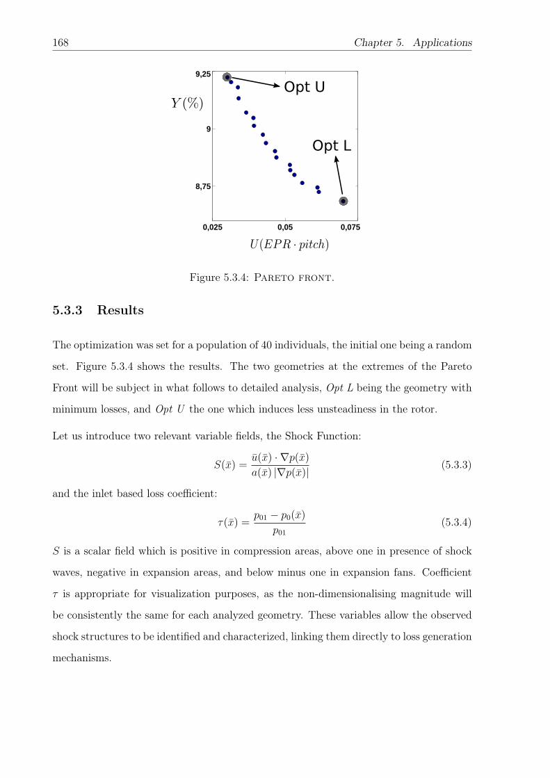
168 Chapter 5. Applications
Opt L
Opt U
Figure 5.3.4: Pareto front.
5.3.3 Results
The optimization was set for a population of 40 individuals, the initial one being a random
set. Figure 5.3.4 shows the results. The two geometries at the extremes of the Pareto
Front will be subject in what follows to detailed analysis, Opt L being the geometry with
minimum losses, and Opt U the one which induces less unsteadiness in the rotor.
Let us introduce two relevant variable fields, the Shock Function:
S(x) =u(x) · ∇p(x)
a(x) |∇p(x)|(5.3.3)
and the inlet based loss coefficient:
τ(x) =p01 − p0(x)
p01
(5.3.4)
S is a scalar field which is positive in compression areas, above one in presence of shock
waves, negative in expansion areas, and below minus one in expansion fans. Coefficient
τ is appropriate for visualization purposes, as the non-dimensionalising magnitude will
be consistently the same for each analyzed geometry. These variables allow the observed
shock structures to be identified and characterized, linking them directly to loss generation
mechanisms.
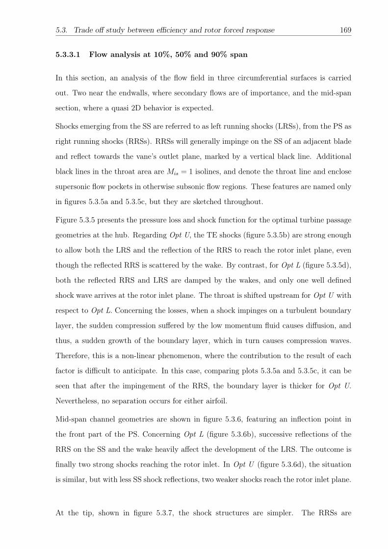
5.3. Trade off study between efficiency and rotor forced response 169
5.3.3.1 Flow analysis at 10%, 50% and 90% span
In this section, an analysis of the flow field in three circumferential surfaces is carried
out. Two near the endwalls, where secondary flows are of importance, and the mid-span
section, where a quasi 2D behavior is expected.
Shocks emerging from the SS are referred to as left running shocks (LRSs), from the PS as
right running shocks (RRSs). RRSs will generally impinge on the SS of an adjacent blade
and reflect towards the vane’s outlet plane, marked by a vertical black line. Additional
black lines in the throat area are Mis = 1 isolines, and denote the throat line and enclose
supersonic flow pockets in otherwise subsonic flow regions. These features are named only
in figures 5.3.5a and 5.3.5c, but they are sketched throughout.
Figure 5.3.5 presents the pressure loss and shock function for the optimal turbine passage
geometries at the hub. Regarding Opt U, the TE shocks (figure 5.3.5b) are strong enough
to allow both the LRS and the reflection of the RRS to reach the rotor inlet plane, even
though the reflected RRS is scattered by the wake. By contrast, for Opt L (figure 5.3.5d),
both the reflected RRS and LRS are damped by the wakes, and only one well defined
shock wave arrives at the rotor inlet plane. The throat is shifted upstream for Opt U with
respect to Opt L. Concerning the losses, when a shock impinges on a turbulent boundary
layer, the sudden compression suffered by the low momentum fluid causes diffusion, and
thus, a sudden growth of the boundary layer, which in turn causes compression waves.
Therefore, this is a non-linear phenomenon, where the contribution to the result of each
factor is difficult to anticipate. In this case, comparing plots 5.3.5a and 5.3.5c, it can be
seen that after the impingement of the RRS, the boundary layer is thicker for Opt U.
Nevertheless, no separation occurs for either airfoil.
Mid-span channel geometries are shown in figure 5.3.6, featuring an inflection point in
the front part of the PS. Concerning Opt L (figure 5.3.6b), successive reflections of the
RRS on the SS and the wake heavily affect the development of the LRS. The outcome is
finally two strong shocks reaching the rotor inlet. In Opt U (figure 5.3.6d), the situation
is similar, but with less SS shock reflections, two weaker shocks reach the rotor inlet plane.
At the tip, shown in figure 5.3.7, the shock structures are simpler. The RRSs are

170 Chapter 5. Applications
LRSRRS
Reflected RRS
BL-Shockinteraction
Wake
Succesivelyreflected RRS
0.0
0.15
0.3
0.9
0.0
-0.9
a) b)
c) d)
Figure 5.3.5: τ and S fields at hub. Top, Opt U. Bottom, Opt L.
a) b)
c) d)
0.0
0.15
0.3
0.9
0.0
-0.9
Figure 5.3.6: τ and S fields at midspan. Top, Opt U. Bottom, Opt L..
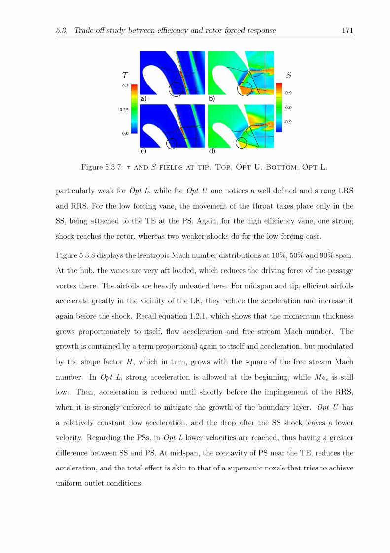
5.3. Trade off study between efficiency and rotor forced response 171
a) b)
c) d)
0.0
0.15
0.3
0.9
0.0
-0.9
Figure 5.3.7: τ and S fields at tip. Top, Opt U. Bottom, Opt L.
particularly weak for Opt L, while for Opt U one notices a well defined and strong LRS
and RRS. For the low forcing vane, the movement of the throat takes place only in the
SS, being attached to the TE at the PS. Again, for the high efficiency vane, one strong
shock reaches the rotor, whereas two weaker shocks do for the low forcing case.
Figure 5.3.8 displays the isentropic Mach number distributions at 10%, 50% and 90% span.
At the hub, the vanes are very aft loaded, which reduces the driving force of the passage
vortex there. The airfoils are heavily unloaded here. For midspan and tip, efficient airfoils
accelerate greatly in the vicinity of the LE, they reduce the acceleration and increase it
again before the shock. Recall equation 1.2.1, which shows that the momentum thickness
grows proportionately to itself, flow acceleration and free stream Mach number. The
growth is contained by a term proportional again to itself and acceleration, but modulated
by the shape factor H, which in turn, grows with the square of the free stream Mach
number. In Opt L, strong acceleration is allowed at the beginning, while Mee is still
low. Then, acceleration is reduced until shortly before the impingement of the RRS,
when it is strongly enforced to mitigate the growth of the boundary layer. Opt U has
a relatively constant flow acceleration, and the drop after the SS shock leaves a lower
velocity. Regarding the PSs, in Opt L lower velocities are reached, thus having a greater
difference between SS and PS. At midspan, the concavity of PS near the TE, reduces the
acceleration, and the total effect is akin to that of a supersonic nozzle that tries to achieve
uniform outlet conditions.
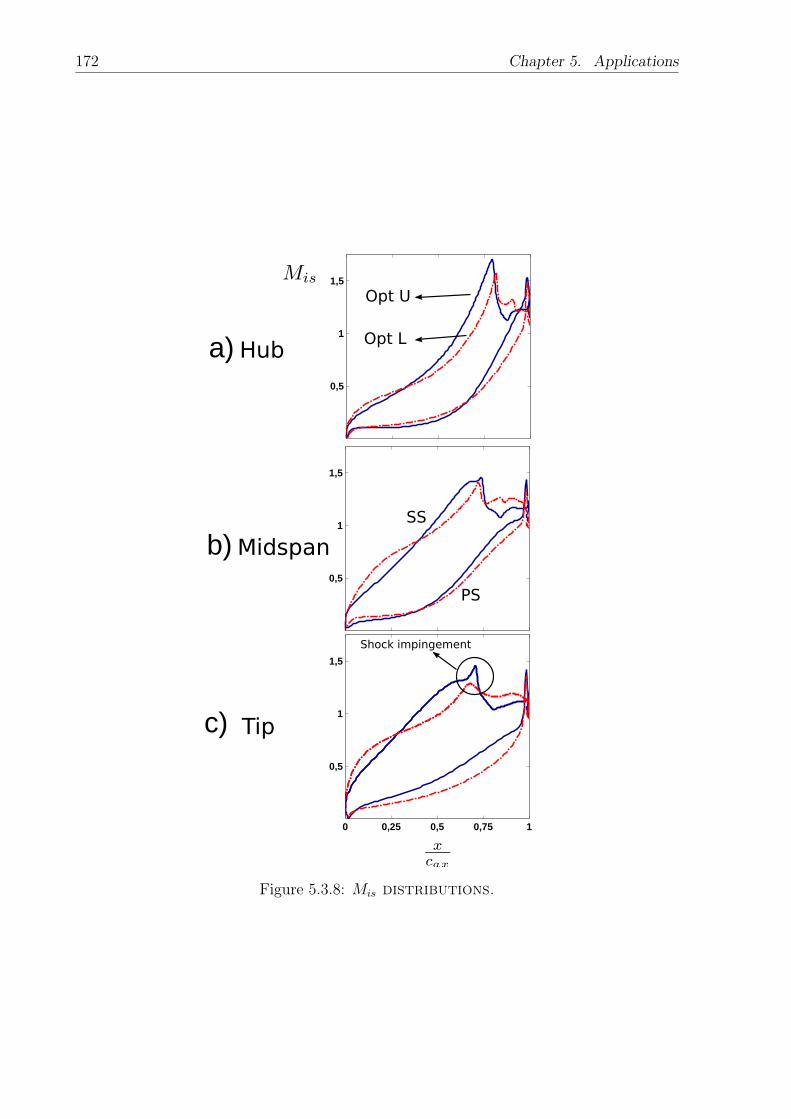
172 Chapter 5. Applications
Opt L
Opt U
a)
b)
c)
Hub
Midspan
Tip
PS
SS
Shock impingement
Figure 5.3.8: Mis distributions.
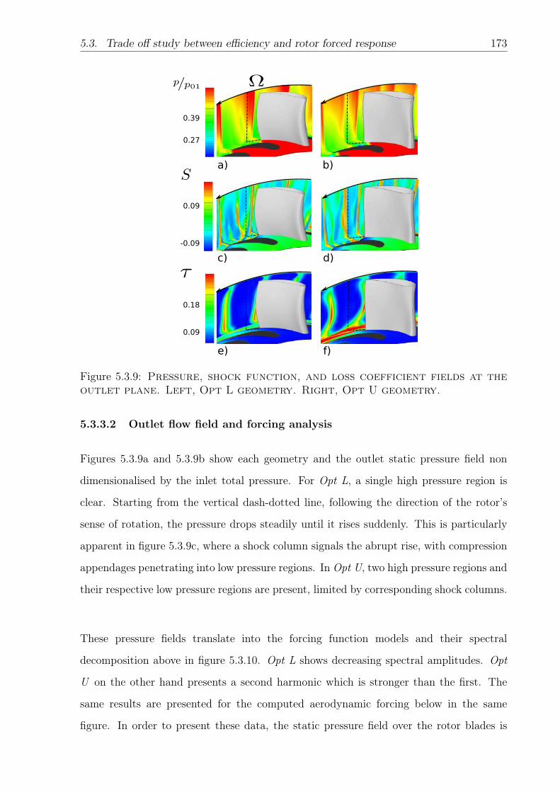
5.3. Trade off study between efficiency and rotor forced response 173
a) b)
c) d)
e) f)
0.39
0.27
0.09
-0.09
0.18
0.09
Figure 5.3.9: Pressure, shock function, and loss coefficient fields at theoutlet plane. Left, Opt L geometry. Right, Opt U geometry.
5.3.3.2 Outlet flow field and forcing analysis
Figures 5.3.9a and 5.3.9b show each geometry and the outlet static pressure field non
dimensionalised by the inlet total pressure. For Opt L, a single high pressure region is
clear. Starting from the vertical dash-dotted line, following the direction of the rotor’s
sense of rotation, the pressure drops steadily until it rises suddenly. This is particularly
apparent in figure 5.3.9c, where a shock column signals the abrupt rise, with compression
appendages penetrating into low pressure regions. In Opt U, two high pressure regions and
their respective low pressure regions are present, limited by corresponding shock columns.
These pressure fields translate into the forcing function models and their spectral
decomposition above in figure 5.3.10. Opt L shows decreasing spectral amplitudes. Opt
U on the other hand presents a second harmonic which is stronger than the first. The
same results are presented for the computed aerodynamic forcing below in the same
figure. In order to present these data, the static pressure field over the rotor blades is
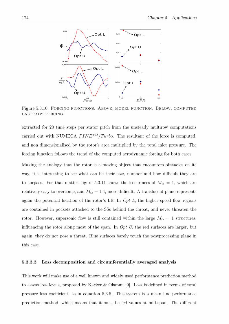
174 Chapter 5. Applications
Opt L
Opt U
Opt U
Opt L Opt L
Opt U
Opt L
Opt U
Figure 5.3.10: Forcing functions. Above, model function. Below, computedunsteady forcing.
extracted for 20 time steps per stator pitch from the unsteady multirow computations
carried out with NUMECA FINETM/Turbo. The resultant of the force is computed,
and non dimensionalised by the rotor’s area multiplied by the total inlet pressure. The
forcing function follows the trend of the computed aerodynamic forcing for both cases.
Making the analogy that the rotor is a moving object that encounters obstacles on its
way, it is interesting to see what can be their size, number and how difficult they are
to surpass. For that matter, figure 5.3.11 shows the isosurfaces of Mis = 1, which are
relatively easy to overcome, and Mis = 1.4, more difficult. A translucent plane represents
again the potential location of the rotor’s LE. In Opt L, the higher speed flow regions
are contained in pockets attached to the SSs behind the throat, and never threaten the
rotor. However, supersonic flow is still contained within the large Mis = 1 structures,
influencing the rotor along most of the span. In Opt U, the red surfaces are larger, but
again, they do not pose a threat. Blue surfaces barely touch the postprocessing plane in
this case.
5.3.3.3 Loss decomposition and circumferentially averaged analysis
This work will make use of a well known and widely used performance prediction method
to assess loss levels, proposed by Kacker & Okapuu [9]. Loss is defined in terms of total
pressure loss coefficient, as in equation 5.3.5. This system is a mean line performance
prediction method, which means that it must be fed values at mid-span. The different
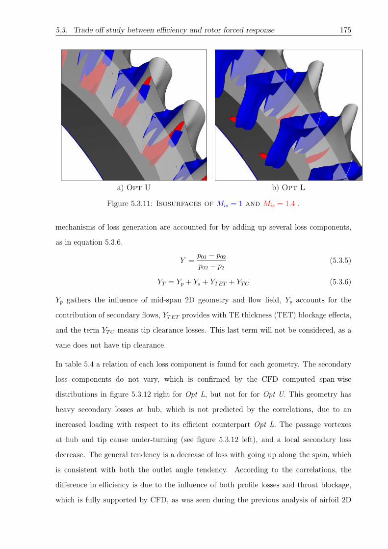
5.3. Trade off study between efficiency and rotor forced response 175
a) Opt U b) Opt L
Figure 5.3.11: Isosurfaces of Mis = 1 and Mis = 1.4 .
mechanisms of loss generation are accounted for by adding up several loss components,
as in equation 5.3.6.
Y =p01 − p02
p02 − p2
(5.3.5)
YT = Yp + Ys + YTET + YTC (5.3.6)
Yp gathers the influence of mid-span 2D geometry and flow field, Ys accounts for the
contribution of secondary flows, YTET provides with TE thickness (TET) blockage effects,
and the term YTC means tip clearance losses. This last term will not be considered, as a
vane does not have tip clearance.
In table 5.4 a relation of each loss component is found for each geometry. The secondary
loss components do not vary, which is confirmed by the CFD computed span-wise
distributions in figure 5.3.12 right for Opt L, but not for for Opt U. This geometry has
heavy secondary losses at hub, which is not predicted by the correlations, due to an
increased loading with respect to its efficient counterpart Opt L. The passage vortexes
at hub and tip cause under-turning (see figure 5.3.12 left), and a local secondary loss
decrease. The general tendency is a decrease of loss with going up along the span, which
is consistent with both the outlet angle tendency. According to the correlations, the
difference in efficiency is due to the influence of both profile losses and throat blockage,
which is fully supported by CFD, as was seen during the previous analysis of airfoil 2D
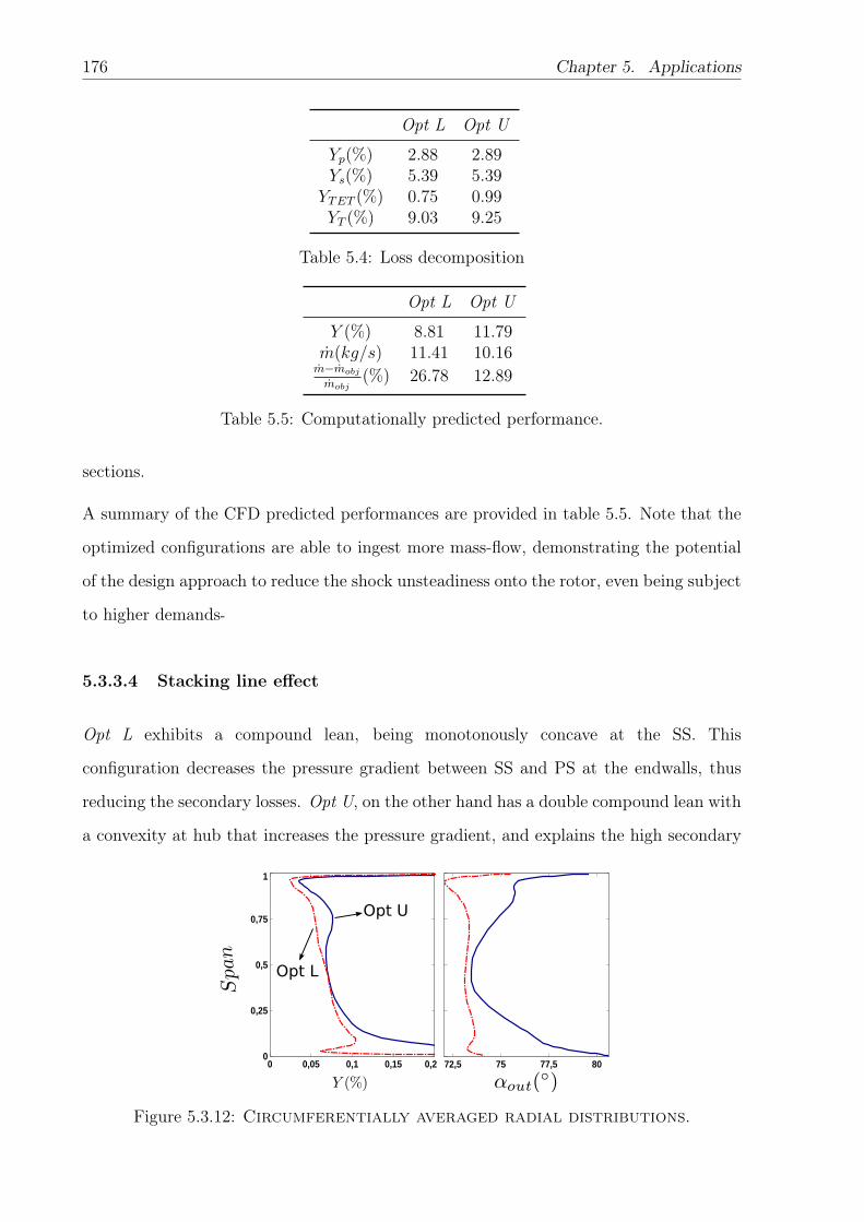
176 Chapter 5. Applications
Opt L Opt U
Yp(%) 2.88 2.89Ys(%) 5.39 5.39YTET (%) 0.75 0.99YT (%) 9.03 9.25
Table 5.4: Loss decomposition
Opt L Opt U
Y (%) 8.81 11.79m(kg/s) 11.41 10.16m−mobj
mobj(%) 26.78 12.89
Table 5.5: Computationally predicted performance.
sections.
A summary of the CFD predicted performances are provided in table 5.5. Note that the
optimized configurations are able to ingest more mass-flow, demonstrating the potential
of the design approach to reduce the shock unsteadiness onto the rotor, even being subject
to higher demands-
5.3.3.4 Stacking line effect
Opt L exhibits a compound lean, being monotonously concave at the SS. This
configuration decreases the pressure gradient between SS and PS at the endwalls, thus
reducing the secondary losses. Opt U, on the other hand has a double compound lean with
a convexity at hub that increases the pressure gradient, and explains the high secondary
Opt U
Opt L
Figure 5.3.12: Circumferentially averaged radial distributions.
5.3. Trade off study between efficiency and rotor forced response 177
losses there. But this increased pressure gradient helps in the development of the strong
shocks that characterize this geometry. In figure 5.3.9, in the lower row, it is seen that
the loss field follows the lean.
5.3.4 Conclusions
A model of unsteady pressure excitations which requires only the steady computation of
the upstream row is presented. This model is physically sound and has been validated
against unsteady multirow computations, which are one order of magnitude higher in
terms of computational expense. However, special care must be taken when defining the
computational domain. The outlet plane should be identical to the postprocessing plane,
located at the axial position of the leading edge of the downstream row.
These tools have been used to generate well performing turbine geometries in terms of
induced rotor forcing and efficiency. Selected geometries from the extreme points of the
Pareto Front of a multiobjective optimization process show how efficiency is lost while
reducing rotor forcing. These geometries are analyzed and the relevant flow features,
such as shock systems and interaction between shocks and viscous flow, are identified and
described. Rotor forcing is reduced by smoothing the static pressure field by means of
increasing the number and reducing the intensity of shocks.
The conclusion is that a great potential for rotor excitation reduction exists while still
achieving high efficiency.

Chapter 6
Conclusions
6.1 Concluding remarks
This thesis has described the development of an Automatic Design Optimization
environment for the aerodynamic design of turbomachinery components, stemming from
an established and validated human driven design system. The main requirements for
such an ADO system were:
• Fast turnaround time: This requirement has motivated the choice of optimization
method (local search, gradient based in order to minimize iterations), the techniques
used for sensitivity computation (adjoint method), and the study of computer
science methods capable of accelerating the required computations (use of GPUs
for general purpose computing). Regarding the choice of optimization algorithms,
the followed approach has been to use established software packages tailored for
the actual purpose, instead of developing a new method from scratch. Actual
optimization algorithms was not the focus of this thesis. Regarding the use of
the adjoint method, theoretical developments on the interpretation and analysis
of the adjoint variables are presented. Finally, with regards to the acceleration
of computations with GPUs, insights are provided on the relationship between
algorithms and hardware architecture, in order to maximize performance.
• Robustness: The design environment must be able to cope with large geometry
variations without failure of the geometry generation methods. This can be helped
179
180 Chapter 6. Conclusions
by careful problem set up, imposing boundaries in the design space, but this
approach does not avoid the need to work on the process of geometry generation
itself. In this thesis, an existing mesh deformation algorithm has been improved and
ported to GPUs, so that it has become the main mesh generation tool, superseding
the standard procedure of building a mesh for each defined geometry.
• Realism: In this thesis, the main focus has been to develop a practical design
tool. For that, the objective functions and constraints need to be the actual
ones that aerodynamicists use. It is not unusual that optimization exercises seen
in literature propose 2D inverse design applications or 3D optimization based on
CFD computed thermodynamic efficiency. The former is too simple an exercise,
and the latter is directly not sound practice, as it is known that CFD does not
compute aerodynamic losses accurately. In addition, there are requirements in a
real industrial design that are usually neglected in literature. The design of a single
row will have constraints trickling down from whole component considerations, and
there are structural and geometrical constraints that need to be considered. In this
work, realistic aerodynamic objectives are considered, including 3D inverse design
for regular flow regions and secondary flows control with several different metrics
(as the problem of secondary flow influence quantification is an open one). Also
complex non-linear geometrical constraints can be considered within the developed
framework, allowing in the end for the obtention of nearly human design quality
solutions. Finally, the obtained solutions are generated using the file formats used
in human driven design, ensuring full compatibility with the workflow within the
company.
Three applications have been shown. The first one presents a trade-off study between
efficiency and rotor forcing for a High Pressure Turbine vane. It is an example of the
performance of evolutionary strategies and their capability to explore the full landscape
of a necessarily reduced (due to the curse of dimensionality) design space. Insights are
extracted on trailing edge shock wave structure interaction with a downstream rotor. It
is shown how the shape of the boundary layer (which is the main contributor to loss, not
the actual shocks) can be tailored to alter the shock structure, diminishing its intensity
6.2. Future work 181
so that the rotor is less affected, but this effect has an associated efficiency penalty. This
study must be considered a theoretical or conceptual one, as the search space was not
constrained enough to ensure production quality solutions. These kind of studies have its
place but that is not the industrial design context.
The second exercise is an initial proof of concept of the application of the ADO system
which is the main subject of this thesis, consisting of the tangential lean optimization
of a compressor Outlet Guide Vane to prevent separation in a downstream S-Shaped
duct. A seamless automatic workflow had already been implemented, communicating
every necessary preprocessing, analysis, and postprocessing tool. However, computations
were still carried out in standard CPUs. Nevertheless, the exercise provided with the
opportunity to delve deeper in the study of adjoint variables. It is shown how adjoints of
flow variables other than the conservative ones can be used to evaluate the convergence
of the optimization process (they show why the process has converged, not merely that
it has), and assist in the physical intuition of the geometrical changes that are needed in
order to improve.
The last example is a rigorous comparison between two human designed Low Pressure
Turbine vanes and two automatically designed ones. Each vane belongs in a different
region of the turbine and presents different design challenges. This exercise was performed
once the the bulk of computations (that is, every iterative solver) was carried out in GPUs.
Additionally, developments on constraint treatment and objective functions had also been
carried out. The results have been satisfactory, with the quality of automatically designed
geometries falling just short of the human designed ones due to insufficient problem
specification. Specifically, multipoint analysis, which is routinely performed by human
designers, was not considered. Nevertheless, acceptable solutions were generated in a
fraction of the time employed by human designers.
6.2 Future work
Two open issues remain at the end of this work. A practical one is the identified need
to include robust design capabilities, specifically, the capability to perform multipoint
182 Chapter 6. Conclusions
analyses. A theoretical one is the ongoing effort to develop theoretical understanding of
secondary flows. Losses due to secondary flows come from diverse mechanisms, and there
is not one single agreed upon metric that characterizes them completely. Merely adding
new metrics may lead to ill posed problems, so there is a need for thorough understanding
of the flow mechanisms involved.
Besides these big picture aspects, in every piece of software there are improvements to be
made, whether in terms of algorithms or capabilities. The current adjoint solver operates
by time marching the spatially discretized residuals. An obvious upgrade is to use a
matrix-free linear solver to accelerate convergence. The current formulation of inlet and
outlet non-reflecting boundary conditions is based on a one dimensional formulation. A
two dimensional formulation needs to be explored. This will open the door to multirow
adjoint computations, as these 2D boundary conditions form the basis for the mixing
plane approach followed by the non-linear solver for steady state multirow calculations.
Finally, the final user may always have feedback on additional objectives or constraints,
of user interface issues which will need to be addressed.
Bibliography
[1] Gisbert, F., 2007. “Resolution of the adjoint Navier-Stokes equations using a
preconditioned multigrid method”. PhD thesis, Escuela Técnica Superior de
Ingenieros Aeronáuticos.
[2] Smith, S. F., 1965. “A simple correlation of turbine efficiency”. The Aeronautical
Journal, 69, pp. 467–470.
[3] Wu, C.-H., 1952. A general theory of three dimensional flow in subsonic and
supersonic turbomachines of axial, radial, or mixed flow types. Technical Note
2604, NACA.
[4] Moody, L. H., 1944. “Friction factors for pipe flow”. In Transactions of the ASME.
[5] Hodson, H. P., and Howell, R. J., 2005. “Bladerow interactions, transition and
high-lift aerofoils in low-pressure turbines”. Annual Review of Fluid Mechanics, 37,
pp. 71–98.
[6] Hodson, H. P., and Dawes, W. N., 1998. “On the interpretation of measured
profile losses in unsteady wake-turbine blade interaction studies”. Journal of
Turbomachinery, 120, pp. 276–284.
[7] Ainley, D. G., and Mathieson, G. C. R., 1951. A method of performance estimation
for axial flow turbines. Tech. rep., British Aeronautical Research Council.
[8] Craig, H. R. M., and Cox, H. J. A., 1970/71. “Performance estimation of axial flow
turbines”. In Proceedings of the Institution of Mechanical Engineers, Vol. 185.
[9] Kacker, S. C., and Okapuu, U., 1982. “A mean line prediction method for axial flow
turbine efficiency”. Journal of Engineering for Power, 104, pp. 111–119.
183
184 Bibliography
[10] Lewis, R. I., 1996. Turbomachinery Performance Analysis. Butterworth-Heinemann.
[11] Coull, J. D., and Hodson, H. P., 2012. “Blade loading and its application in the
mean-line design of low pressure turbines”. Journal of Turbomachinery, 135(2),
pp. 021032–021032–12.
[12] Bertini, F., Ampellio, E., and Marconcini, M., 2013. “A critical numerical review of
loss correlation models and smith diagram for modern low pressure turbine stages”.
In Proceedings of ASME TurboExpo, no. GT2013-94849.
[13] Hernández, D., Antoranz, A., and Vázquez, R., 2013. “Application of smith chart
for non repeating stages in axial compressors”. In Proceedings of ASME TurboExpo,
no. GT2013-94199.
[14] Pacciani, R., Marconcini, M., and Arnone, A., 2017. “A cfd-based throughflow
method with three-dimensional flow features modeling”. International Journa of
Turbomachinery Propulsion and Power, 2(3)(11), p. 12.
[15] Hirsch, C., and Denton, J. D., 1976. “Through-flow calculations in axial
turbomachinery”. In AGARD Conference Proceedings, no. 195.
[16] Denton, J. D., and Dawes, W. N., 1998. “Computational fluid dynamics for
turbomachinery design”. Journal of Mechanical Engineering Science, 213, pp. 107–
124.
[17] Gannon, A. J., and von Backström, T. W., 1998. “A comparison of the streamline
throughflow and streamline curvature methods for axial turbomachinery”. In
Proceedings of the International Gas Turbine and Aeroengine Congress, no. 98-
GT-48.
[18] Persico, G., and Rebay, S., 2012. “A penalty formulation for the throughflow
modeling of turbomachinery”. Computers & Fluids, 60, pp. 86–98.
[19] Roache, P. J., 1998. Verification and Validation in Computational Science and
Engineering. Hermosa Pub.

Bibliography 185
[20] Wilcox, D. C., 1994. Turbulence Modeling for CFD. DCW Industries, Inc., La
Cañada, California.
[21] Denton, J. D., 2010. “Some limitations of turbomachinery CFD”. In Proceedings of
ASME TurboExpo, no. GT2010-22540.
[22] Denton, J. D., 1993. “Loss mechanisms in turbomachines”. Journal of
Turbomachinery, 115, pp. 621–656.
[23] Thompson, B. G. J., 1967. A critical review of existing methods of calculating the
turbulent boundary layer. Reports and memoranda 3447, Aeronautical Research
Council.
[24] Jiménez, J., 2004. “Turbulent flows over rough walls”. Annual Review of Fluid
Mechanics, 36, pp. 173–196.
[25] Vázquez, R., and Torre, D., 2013. “The effect of surface roughness on efficiency of
low pressure turbines”. Journal of Turbomachinery, 136(6), pp. 061008–061008–7.
[26] Volino, R. J., 2003. “Passive flow control on low-pressure turbine airfoils”. Journal
of Turbomachinery, 125, p. 754.
[27] Sieverding, C. H., 1985. “Recent progress in the understanding of basic aspects of
secondary flows in turbine blade passages”. Journal of Engineering for Gas Turbines
and Power, 107, pp. 248–257.
[28] Wennerstrom, A., ed., 1989. Secondary Flows in Turbomachinery, Advisory Group
for Aerospace Research and Development.
[29] Duden, A., Raab, I., and Fottner, L., 1999. “Controlling the secondary flow in a
turbine cascade by three-dimensional airfoil design and endwall contouring”. Journal
of Turbomachinery, 121, pp. 191–207.
[30] Torre, D., Vázquez, R., de la R. Blanco, E., and Hodson, H. P., 2006. “A new
alternative for reduction of secondary flows in low pressure turbines”. Journal of
Turbomachinery, 133, p. p. 011029.
186 Bibliography
[31] Corral, R., and Gisbert, F., 2008. “Profiled end wall design using an adjoint Navier-
Stokes solver”. Journal of Turbomachinery, 130(2), pp. 1–8.
[32] Prümper, H., 1972. “Application of boundary layer fences in turbomachinery”.
AGARDograph, 164, pp. 311–331.
[33] Kumar, K. N., and Govardhan, M., 2011. “Secondary loss reduction in a turbine
cascade with a linearly varied height streamwise endwall fence”. Journal of Rotating
Machinery, 2011, p. 16.
[34] Sauer, H., Müller, R., and Vogeler, K., 2000. “Reduction of secondary flow losses
in turbine cascades by leading edge modifications at the endwall”. Journal of
Turbomachinery, 123, pp. 207–213.
[35] Lei, Q., Zhenping, Z., Peng, W., Teng, C., and Huoxing, L., 2011. “Control of
secondary flow loss in turbine cascade by streamwise vortex”. Computers & Fluids,
54, pp. 45–55.
[36] Lewis, R. I., and Hill, J. M., 1971. “The influence of sweep and dihedral in
turbomachinery blade rows”. Journal of Mechanical Engineering Science, 13,
pp. 266–285.
[37] Pullan, G., and Harvey, N. W., 2006. “The influence of sweep on axial flow turbine
aerodynamics at mid-span”. Journal of Turbomachinery, 129, pp. 591–598.
[38] Pullan, G., and Harvey, N. W., 2008. “The influence of sweep on axial flow turbine
aerodynamics in the endwall region”. Journal of Turbomachinery, 130, pp. 041011–
10.
[39] Lázaro, B. J., González, E., and R.Vázquez, 2008. “Temporal structure of
the boundary layer in low reynolds number, low pressure trubine profiles”. In
Proceedings of ASME Turbo Expo, no. GT2008-50616.
[40] Lázaro, B. J., González, E., and R.Vázquez, 2007. “Unsteady loss production
mechanisms in low reynolds number, high lift, low pressure turbine profiles”. In
Proceedings of ASME Turbo Expo, no. GT2007-28142.
Bibliography 187
[41] Tyler, J. M., and Sofrin, T. G., 1962. “Axial flow compressor noise studies”.
Transactions of the Society of Automotive Engineers, 70, pp. 309–332.
[42] Vázquez, R., Torre, D., and Serrano, A., 2013. “The effect of airfoil clocking on
efficiency and noise of low pressure turbines”. Journal of Turbomachinery, 136(6),
p. 061006.
[43] Woodward, R. P., Elliot, D. M., Hughes, C. E., and Berton, J. J., 1998. Benefits of
swept and leaned stators for fan noise reduction. Tech. Rep. 1998-208661, NASA.
[44] Coull, J. D., Thomas, R. L., and Hodson, H. P., 2010. “Velocity distributions for
low pressure turbines”. Journal of Turbomachinery, 132, p. 041006.
[45] Zoric, T., Popovic, I., Sjolander, S. A., Praisner, T., and Grover, E., 2007.
“Comparative investigation of three highly loaded lp turbine airfoils: Part i -
measured profile and secondary losses at design incidence”. In Proceedings of ASME
Turbo Expo, no. GT2007-27537.
[46] Zoric, T., Popovic, I., Sjolander, S. A., Praisner, T., and Grover, E., 2007.
“Comparative investigation of three highly loaded lp turbine airfoils: Part ii -
measured profile and secondary losses at off-design incidence”. In Proceedings of
ASME Turbo Expo, no. GT2007-27538.
[47] Torre, D., Vázquez, R., Armañanzas, L., Partida, F., and García-Valdecasas, G.,
2013. “The effect of airfoil thickness on the efficiency of LP turbines”. Journal of
Turbomachinery, 136, p. p. 051014.
[48] Joly, M., Verstraete, T., and Paniagua, G., 2013. “Differential evolution based soft
optimization to attenuate vane-rotor shock interaction in high-pressure turbines”.
Applied Soft Computing, 13, pp. 1882–1891.
[49] Blickle, T., and Tiele, L., 1995. A comparison of selection schemes used in genetic
algorithms. Tik-report, Swiss Federal Institute of Technology (ETH), Computer
Engineering and Communications Network Lab.
188 Bibliography
[50] Konaka, A., Coitb, D. W., and Smith, A. E., 2005. “Multi-objective optimization
using genetic algorithms: A tutorial”. Realiability Engineering and Systems Safety,
91, pp. 992–1007.
[51] Holland, J. H., 1975. Adaptation in Natural and Artificial Systems. MIT Press.
[52] Price, K., and Storn, N., 1997. Differential evolution- a simple and efficient adaptive
scheme for global optimization over continuous spaces. Tech. Rep. TR-95-012,
University of California.
[53] Kennedy, J., and Eberhart, R., 1995. “Particle swarm optimization”. In Proceedings
of IEEE International Conference on Neural Networks, pp. 1942–1948.
[54] Montgomery, D. C., 1997. Design and Analysis of Experiments. Arizona State
University.
[55] McCulloch, W. S., and Pitts, W., 1990. “A logical calculus of ideas immanent in
nervous activity”. Bulletin of Mathematical Biology, 52, pp. 99–115.
[56] Livieris, I. E., and Pintelas, P., 2008. A survey on algorithms for training artificial
neural networks. Tech. Rep. TR08-01, University of Patras.
[57] Krige, D. G., 1951. “A statistical approach to some basic mine valuation problems
on the witwatersrand”. Journal of the Chemical, Metallurgical and Mining Society
of South Africa, 52, pp. 119–139.
[58] Matheron, G., 1963. “Principles of geostatistics”. Economic Geology, 58, pp. 1246–
1266.
[59] Torczon, V., and Trosset, M. W., 1998. “Using approximations to accelerate engin-
eering design optimization”. In Proceedings of the 7th AIAA/USAF/NASA/ISSMO
Symposium on Multidisciplinary Analysis and Optimization, no. AIAA-98-4800.
[60] Von Karman Institute for Fluid Dynamics, 2010. Introduction to
Optimization and Multidisciplinary Design in Aeronautics and Turbomachinery.

Bibliography 189
[61] de Baar, J. H. S., Dwight, R. P., and Bijl, H., 2014. “Improvements to gradient-
enhanced kriging usisng a bayesian interpretation”. International Journal for
Uncertainty Quantification, 4, pp. 205–223.
[62] Laurenceau, J., and Sagaut, P., 2008. “Building efficient response surfaces of
aerodynamic functions with kriging and cokriging”. AIAA Journal, 46, pp. 498–507.
[63] Belyaev, M., Burnaev, E., Kapushev, E., Panov, M., Prikhodko, P., Vetrov, D., and
Yarotsky, D., 2016. “Gtapprox: Surrogate modeling for industrial design”. Advances
in Engineering Software, 102, pp. 29–39.
[64] Gano, S. E., Kim, H., and Brown, D. E., 2006. “Comparison of three surrogate
modelling techniques: Datascape®, kriging and second order regression”. In 11th
AIAA/ISSMO Multidisciplinary Analysis and Optimization Conference, no. AIAA-
2006-7048.
[65] Kolda, T. G., Lewis, R. M., and Torczon, V., 2003. “Optimization by direct search:
New perspectives on some classical and modern methods”. SIAM Review, 45,
pp. 385–482.
[66] Torczon, V., 1991. “On the convergence of the multidirectional search algorithm”.
SIAM Journal of Optimization, 1, pp. 123–145.
[67] Nelder, J. A., and Mead, R., 1965. “A simplex method for function minimization”.
Computer Journal, 7, pp. 308–313.
[68] Custódio, A. L., and Vicente, L. N., 2007. “Using sampling and simplex derivatives
in pattern search methods”. SIAM Journal of Optimization, 18, pp. 537–555.
[69] Gould, N., 2006. An introduction to algorithms for continuous optimization.
[70] Gilbert, J. C., 1987. On the local and global convergence of a reduced quasi-newton
method. Tech. rep., International Institute for Applied Systems Analysis.
[71] Rockafellar, R. T., 1993. “Lagrangemultipliers and optimality”. SIAM Review, 35,
pp. 183–238.
190 Bibliography
[72] Verstraete, T., 2008. “Multidisciplinary optimization of turbomachinery components
including heat transfer and stress predictions”. PhD thesis, Universiteit Gent.
[73] Runarsson, T. P., and Yao, X., 2005. “Search biases in constrained evolutionary
optimization”. IEEE Transactions on Systems, Man and Cybernetics-Part C:
Applications and Reviews, 35, pp. 233–243.
[74] Wächter, A., and Biegler, L. T., 2004. “On the implementation of an interior point
filter line search algorithm for large scale nonlinear programming”. Mathematical
Programming, 106, pp. 25–57.
[75] Chattopadhyay, A., and Rajadas, J. N., 1998. An enhanced multi-objective
optimization technique for comprehensive aerospace design. Tech. rep., Arizona
State University.
[76] Chattopadhyay, A., and McCarthy, T. R., 1994. “An optimization procedure for the
design of prop-rotors in high speed cruise including the coupling of performance,
aeroelastic stability, and structures.”. Journal of Mathematical Computational
Modelling, 19(3), pp. 75–88.
[77] Grodzevich, O., and Romanko, O., 2006. “Normalization and other topics in multi-
objective optimization”. In Proceedings of the Fields-MITACS Industrial Problems
Workshop.
[78] Marler, R. T., and Arora, J. S., 2004. “Survey of multi-objective optimization
methods for engineering”. Structural Multidisciplinary Optimization, 26(6), pp. 369–
395.
[79] Messac, A., 1996. “Physical programming: Effective optimization for computational
design”. AIAA Journal, 34, pp. 149–158.
[80] Chircop, K., and Zammit-Mangion, D., 2013. “On ε-constraint based methods
for the generation of pareto frontiers”. Journal of Mechanics Engineering and
Automation, 3, pp. 279–289.
[81] Lele, S. K., 1992. “Compact finite difference schemes with spectral-like resolution”.
Journal of Computational Physics, 103, pp. 16–42.
Bibliography 191
[82] Lai, K., and Crassidis, J. L., 2008. “Extensions of the first and second complex-step
derivative approximations”. Journal of Computational and Applied Mathematics,
219(1), pp. 276–293.
[83] Lantoine, G., Russell, R. P., and Dargent, T., 2012. “Using multicomplex variables
for automatic computation of high-order derivatives”. ACM Transactions on
Mathematical Software, 38, pp. –.
[84] Griewank, A., and Walther, A., 2008. Evaluating Derivatives: Principles and
Techniques of Algorithmic Differentiation. Society for Industrial and Applied
Mathematic.
[85] Wagner, M., Walther, A., and Schäfer, B. J., 2009. “On the efficient computation
of high-order derivatives for implicitly defined functions”. Computer Physics
Communications, 181, pp. 756–764.
[86] Giles, M. B., 2000. “An introduction to the adjoint approach to design”. Flow,
Turbulence and Combustion, 65(3), pp. 393–415.
[87] Nadarajah, S. K., and Jameson, A., 2000. “A comparison of the continuous and
discrete adjoint approach to automatic aerodynamic optimization”. In Proceedings
of the AIAA Aerospace Sciences Meeting and Exhibit, no. AIAA-2000-0667.
[88] Arian, E., and Salas, M. D., 1997. Admitting the inadmissible: Adjoint formulation
for incomplete cost functionals in aerodynamic design. Tech. rep., NASA Langley
Research Center.
[89] Cusdin, P., and Müller, J.-D., 2003. Deriving linear and adjoint codes for CFD
using automatic differentiation.
[90] Giles, M. B., Gate, D., and Duta, M. C., 2006. “Using automatic differentiation
for adjoint CFD code development”. In Recent Trends in Aerospace Design and
optimization, pp. 426–434.
[91] Hascoët, L., and Dauvergne, B. Adjoints of large simulation codes through
automatic differentiation.
192 Bibliography
[92] Jones, D., Christakopoulos, F., and Muller, J. D., 2010. “Adjoint CFD codes
through automatic differentiation”. In European Conference on Computational
Fluid Dynamics.
[93] Duta, M. C., Shahpar, S., and Giles, M. B., 2007. “Turbomachinery design
optimization using automatic differentiated adjoint code”. In Proceedings of ASME
Turbo Expo, no. GT2007-28329.
[94] Martinelli, M., Dervieux, A., and Hascöet, L., 2007. “Strategies for computing
second order derivatives in CFD design problems”. In Proceedings of the West-East
High Speed Flow Field Coference.
[95] Rumpfkeil, M. P., and Mavriplis, D. J., 2010. “Efficient hessian calculations using
automatic differentiation and the adjoint method with applications”. AIAA Journal,
48, pp. 2406–2417.
[96] Papapadimitrou, D. I., and Giannakoglou, K. C., 2010. “One-shot shape
optimization using the exact hessian”. In European Conference on Computational
Fluid Dynamics.
[97] Griewank, A., 2006. Projected Hessians for Preconditioning in One-Step One-Shot
Design Optimization". Springer US, Boston, MA, pp. 151–171.
[98] Günther, S., Gauger, N. R., and Wang, Q., 2016. “Simultaneous single-step one-
shot optimization with unsteady pdes”. Journal of Computational and Applied
Mathematics, 294, pp. 12–22.
[99] Hazra, S., 2012. “Multigrid one-shot method for pde-constrained optimization
problems”. Applied Mathematics, 3(10A), pp. 1565–1571.
[100] Shahpar, S., 2011. “Challenges to overcome for routine usage of automatic
optimisation in the propulsion industry”. The Aeronautical Journal, 115(1172),
pp. 615–625.
[101] Shahpar, S., 2005. “Sophy: An integrated cfd based automatic design system”. In
International Symposium on Air Breathing Engines, no. ISABE-2005-1086.
Bibliography 193
[102] Verstraete, T., 2010. “Cado: A computer aided design and optimization tool for
turbomachinery applications”. In Proceedings of the 2nd International Conference
on Engineering Optimization.
[103] Siller, U., Voss, C., and Nicke, E., 2009. “Automated multidisciplinary optimization
of a transonic axial compressor”. In Proceedings of the AIAA Aerospace Sciences
Meeting, no. AIAA-2009-863.
[104] Glowinski, R., and Pironneau, O., 1976. “Towards the computation of minimum
drag profiles in viscous laminar flow”. Journal of Applied Mathematical Modeling,
1(2), pp. 58–66.
[105] Jameson, A., 1995. Computational Fluid Dynamics Review. No. ISBN 0-471-95589-
2. Wiley, ch. Optimum Aerodynamic Design Using Control Theory, pp. 495–528.
[106] Martins, J. R. R. A., Alonso, J. J., and Reuther, J. J., 2005. “A coupled-adjoint
sensitivity analysis method for high-fidelity aero-structural design”. Journal of
Optimization and Engineering, 6(1), pp. 33–62.
[107] Duta, M. C., Giles, M. B., and Campobasso, M. S., 2002. “The harmonic adjoint
approach to unsteady turbomachinery design”. International Journal for Numerical
Methods in Fluids, 40(3-4), pp. 323–332.
[108] Benini, E., 2005. “Three-dimensional multi-objective design optimization of a
transonic compressor rotor”. Journal of Propulsion and Power, 20(3), pp. 559–565.
[109] Okui, H., Verstraete, T., Braembussche, R. A., and Alsalihi, Z., 2011. “Three-
dimensional design and optimization of a transonic rotor in axial flow compressors”.
Journal of Turbomachinery, 135(3), p. 031009.
[110] Wang, D. X., and He, L., 2010. “Adjoint aerodynamic design optimization for blades
in multistage turbomachines”. Journal of Turbomachinery, 132(2), pp. 021011/1–
14.
[111] Walther, B., and Nadarajah, S. K., 2015. “Adjoint based constrained aerodynamic
shape optimization for multistage turbomachines”. Journal of Propulsion and
Power, 31(5), pp. 1298–1319.
194 Bibliography
[112] Li, H., Song, L., Li, Y., and Feng, Z., 2010. “2d viscous aerodynamic
shape optimization for turbine blades based on adjoint method”. Journal of
Turbomachinery, 133(3), pp. 031014–8.
[113] Wang, D. X., and Li, Y. S., 2010. “3d direct and inverse design using n-s equations
and the adjoint method for turbine blades”. In Proceedings of ASME TurboExpo,
no. GT2010-22049.
[114] van Rooij, M. P. C., Dang, T. Q., and Larosiliere, L. M., 2005. “Improving
aerodynamic matching of axial compressor blading using a three-dimensional
multistage inverse design method”. Journal of Turbomachinery, 129(1), pp. 108–
118.
[115] Mayle, R. E., 1991. “The igti scholar lecture: The role of laminar-turbulent
transition in gas turbine engines”. Journal of Turbomachinery, 113(4), p. 28.
[116] Walker, G. J., 1993. “The role of laminar-turbulent transition in gas turbine engines:
A discussion”. Journal of Turbomachinery, 115(2), pp. 2017–216.
[117] Drela, M., 1998. Frontiers in Computational Fluid Dynamics. World Scientific
Publishing, Co, ch. Pros and Cons of Airfoil Optimization, pp. 363–381.
[118] Chen, W., Allen, J. K., Tsui, K.-L., and Mistree, F., 1996. “A procedure for robust
design: Minimizing variations caused by noise factors and control factors”. Journal
of Mechanical Design, 118, pp. 478–487.
[119] Beyer, H.-G., and Senhoff, B., 2007. “Robust optimization-a comprehensive survey”.
Computer Methods in Applied Mechanics and Engineering, 196, pp. 3190–3218.
[120] Kumar, A., Nair, P. B., Keane, A. J., and Shahpar, S., 2007. “Robust design using
bayesian monte carlo”. International Journal for Numerical Methods in Engineering,
73(11), pp. 1497–1517.
[121] Xiu, D., 2009. “Fast numerical methods for stochastic computations: A review”.
Communications in Computational Physics, 5(2-4), pp. 242–272.
Bibliography 195
[122] Dodson, M., and Parks, G. T., 2009. “Robust aerodynamic design optimization
using polynomial chaos”. Journal of Aircraft, 46(2), pp. 635–646.
[123] Shankaran, S., and Marta, A. C., 2012. “Robust optimization for aerodynamic
problems using polynomial chaos and adjoints”. In Proceedings of ASME
Turboexpo, no. GT2012-69580.
[124] Corral, R., and Pastor, G., 2004. “Parametric design of turbomachinery airfoils using
highly differentiable splines”. Journal of Propulsion and Power, 20(2), pp. 335–343.
[125] Drela, M., and Giles, M. B., 1987. “Viscous-inviscid analysis of transonic and low
reynolds number airfoils”. AIAA Journal, 20(10), pp. 1347–1355.
[126] Burgos, M. A., Chía, J. M., Corral, R., and López, C., 2009. “Rapid meshing
of turbomachinery rows using semi-unstructured multi-block conformal grids”.
Engineering with Computers, 26(4), pp. 351–362.
[127] Corral, R., Gisbert, F., and Pueblas, J., 2017. “Execution of a parallel edge-
based Navier-Stokes equations solver on commodity graphics processor units”.
International Journal of Computational Fluid Dynamics, 31(2), pp. 0–16.
[128] Burgos, M. A., Contreras, J., and Corral, R., 2007. “Efficient edge based rotor/stator
interaction method”. AIAA Journal, 49, pp. 19–31.
[129] Zingg, D. W., Nemec, M., and Pulliam, T. H., 2008. “A comparative evaluation of
genetic and gradient based algorithms applied to aerodynamic optimization”. Revue
Européene de Mécanique Numérique, 17, pp. 103–126.
[130] Steffen, M., 1990. “A simple method for monotonic interpolation in one dimension”.
Astronomy and Astrophysics, 239, pp. 443–450.
[131] Moinier, P., 1999. “Algorithm developments for an unstructured viscous flow solver”.
PhD thesis, University of Oxford.
[132] Baldwin, B. S., and Lomax, H., 1978. “Thin layer approximation and algebraic
model for separated trubulent flows”. In AIAA Aerospace Science Meeting, no. AIAA
78-257.
196 Bibliography
[133] Spalart, P. R., and Allmaras, S. R., 1992. “A one-equation turbulence model for
aerodynamic flows”. In 30th Aerospace Science Meeting and Exhibit, no. AIAA
92-0439.
[134] Langtry, R. B., and Menter, F. R., 2009. “Correlation-based transition modeling
for unstructured parallelized computational fluid dynamics codes”. AIAA Journal,
47(12), pp. 2894–2906.
[135] Gisbert, F., and Corral, R., 2009. “Prediction of separation-induced transition using
a correlation-based transition model”. In 9th AIAA Computational Fluid Dynamics
Conference, Vol. AIAA 2009-3666.
[136] Jameson, A., Schmidt, W., and Turkel, E., 1981. “Numerical solutions of the euler
equations by finite volume methods using runge-kutta time-stepping schemes”. In
14th Fluid and Plasma Dynamic Conference, no. AIAA 81-1259.
[137] Roe, P. L., 1981. “Approximate riemann solvers, parameters, vectors and difference
schemes”. Journal of Computational Physics, 43(2), pp. 357–372.
[138] Swanson, R. C., and Turkel, E., 1992. “On central-difference and upwinding
schemes”. Journal of Computational Physics, 101, pp. 292–306.
[139] Xu, S., Jahn, W., and Müller, J.-D., 2013. “Cad-based shape optimisation with cfd
using a discrete adjoint”. International Journal for Numerical Methods in Fluids,
74(3), pp. 153–168.
[140] Martel, C., 2000. Nonlinear constrained optimization of turbomachinery problems.
Tech. rep., Escuela Técnica Superior de Ingenieros Aeronáuticos.
[141] Shankaran, S., Marta, A., Barr, B., Venugopal, P., and Wang, Q., 2012.
“Interpretation of adjoint solutions for turbomachinery flows”. AIAA Journal, 51,
pp. 1733–1744.
[142] Mpi official website.
[143] Karypis, G. Parmetis - parallel graph partitioning and fill-reducing matrix ordering.
Bibliography 197
[144] Larsen, E., and McAllister, D., 2001. “Fast matrix multiplies using graphics
hardware”. In Proceedings of the 2001 ACM/IEEE Conference on Supercomputing.
[145] Du, P., Weber, R., Luszczeck, P., Tomov, S., Peterson, G., and Dongarra, J.,
2011. “From CUDA to OpenCL: Towards a performance portable solution for multi-
platform GPU programming”. Parallel Computing, 38(8), pp. 391–407.
[146] Reguly, I. Z., Mudalige, G. R., Bertoli, C., Giles, M. B., Betts, A., Kelly, P. H., and
Rodford, D., 2013. “Acceleration of a full-scale industrial cfd application with op2”.
IEEE Transactions on Parallel and Distributed Systems, 99(5), pp. 1265–1278.
[147] Brandvik, T., and Pullan, G., 2010. “An accelerated 3d Navier-Stokes solver for
flows in turbomachines”. Journal of Turbomachinery, 12(2), p. 021025.
[148] Gisbert, F., Corral, R., and Pastor, G., 2011. “Implementation of an edge-
based Navier-Stokes solver for unstructured grids in graphics processing units”. In
Proceedings of ASME Turbo Expo, no. GT2011-46224.
[149] Cuthill, E., and McKee, J., 1969. “Reducing the bandwith of sparse symmetric
matrices”. In Proceedings of the 1969 24th ACM National Conference, pp. 157–172.
[150] Castonguay, P., Williams, D., Vincent, P., López, M., and Jameson, A., 2010.
“On the development of a high-order, multi-gpu enabled, compressible viscous flow
solver for mixed unstructured grids”. In 20th AIAA Computational Fluid Dynamics
Conference,.
[151] Corrigan, A., Camelli, F., Löhner, R., and Mut, F., 2010. “Semi-automatic porting
of a large-scale fortran cfd code to gpus”. International Journal for Numerical
Methods in Fluids, 69(2), pp. 314–331.
[152] Contreras, J., Corral, R., Fernández-Castañeda, J., Pastor, G., and Vasco, C., 2002.
“Semi-unstructured grid methods for turbomachinery applications”. In Proceedings
of ASME Gas Turbine and Aeroengine Congress, no. GT2002-30572.
[153] Wang, Y., Qin, N., and Zhao, N., 2015. “Delaunay graph and radial basis function
for fast quality mesh deformation”. Journal of Computational Physics, 294, pp. 149–
172.
198 Bibliography
[154] Warren, J., Schaefer, S., Hirani, A. N., and Desbrun, M., 2006. “Barycentric
coordinates for convex sets”. Advances in Computational Mathematics, 27(3),
pp. 319–338.
[155] Patel, V., and Sotiropoulos, F., 1997. “Longitudinal curvature effects in turbulent
boundary layers”. Progress in Aerospace Sciences, 33, pp. 1–70.
[156] Ortiz, C., Miller, R. J., Hodson, H. P., and Longley, J. P., 2007. “Effect of length
on compressor inter-stage duct performance”. In Proceedings of ASME Turboexpo,
no. GT2007-27752.
[157] Wellborn, S. R., Reichert, B. A., and Okiishi, T. H., 1994. “Study of the compressible
flow in a diffusing S-duct”. Journal of Propulsion and Power, 10, pp. 668–675.
[158] Lee, G. G., Allan, W. D. E., and Boulama, K. G., 2013. “Flow and performance
characteristics of an allison 250 gas turbine S-shaped diffuser: Effects of geometry
variations”. International Journal of Heat and Fluid Flow, 42, pp. 151–163.
[159] Zierer, T., 1995. “Experimental investigation of the flow in diffusers behind an axial
flow compressor”. Journal of Turbomachinery, 117, pp. 231–239.
[160] Walker, A. D., Barker, A. G., Carotte, J. F., Bolger, J. J., and Green, M. J., 2012.
“Integrated outlet guide vane design for an aggresive S-shaped compressor transition
duct”. Journal of Turbomachinery, 135, pp. 11–35.
[161] Giles, M. B., 1997. “Adjoint equations in CFD: Duality, boundary conditions and
solution behaviour”. In 13th Computational Fluid Dynamics Conference, no. AIAA-
97-1850.
[162] Gbadebo, S. A., Cumpsty, N., and Hynes, T. P., 2005. “Three-dimensional
separations in axial compressors”. Journal of Turbomachinery, 127, pp. 331–339.
[163] Li, H. D., and He, L., 2005. “Blade aerodynamic damping variation with rotor-
stator gap: A computational study using single-passage approach”. Journal of
Turbomachinery, 127, pp. 573–579.
Bibliography 199
[164] Li, H. D., and He, L., 2005. “Towards intra-row gap optimization for one and a half
stage transonic compressor”. Journal of Turbomachinery, 127, pp. 589–598.
[165] Paniagua, G., 2002. “Investigation of the steady and unsteady performance of a
transonic hp turbine”. PhD thesis, Université Libre de Bruxelles.
[166] Payne, S. J., 2001. “Unsteady loss in a high pressure turbine stage”. PhD thesis,
University of Oxford.
[167] Barter, J. W., Chen, J. P., and Vitt, P. H., 2000. “Interaction effects in a transonic
turbine stage”. In Proceedings of the ASME TurboExpo, ASME, ed., Vol. 2000-
GT-0376.
[168] Kammerer, A., and Abhari, R. S., 2009. “Blade forcing function and aerodynamic
work measurements in a high speed centrifugal compressor with inlet distortion”. In
Proceedings of the ASME TurboExpo.
[169] Vascellari, M., Dénos, R., and den Braembussche, R. V., 2004. “Design of a transonic
high-pressure turbine stage 2d section with reduced rotor/stator interaction”. In
Proceedings of the ASME TurboExpo, ASME, ed., Vol. GT2004-53520.
[170] Pierret, S., 1999. “Designing turbomachinery blades by means of the function
approximation concept based on artificial neural networks, genetic algorithm, and
the Navier-Stokes equations”. PhD thesis, Falculté Polytechnique de Mons.
[171] Arnone, A., Liou, M. S., and Povinelli, L. A., 1995. “Integration of Navier-Stokes
equations using dual time stepping and a multigrid method”. AIAA, 33, pp. 985–
990.
[172] Wilquem, F., 2008. FINE Turbo v8 Manual: Unsteady Treatment, Non-Linear
Harmonic Method. NUMECA International.

Appendix A
Analytical derivation of cost function
flow sensitivities.
In order to build the forcing term for the adjoint system (∂f/∂u in equation 3.2.4), the
sensitivities of each possible flow dependent objective and constraint function need to be
analytically derived. In this appendix a catalog of the derivations made use of in the course
of this thesis is compiled, including flow magnitudes and scalarizing operators, which
translate somehow field values into a single scalar. Turbulent variables are not considered
in these derivations as the current version of the adjoint code assumes a frozen eddy
viscosity. In case the turbulence models were to be considered in the adjoint equations,
it would be worthwhile to consider the sensitivity of objective functions to turbulent
variables. Also, as the adjoint solver is derived from the RANS equations in conservative
form, the independent variables are the conservative flow variables:
u =
ρ
ρu
ρv
ρw
ρE
(A.0.1)
201
202 Appendix A. Analytical derivation of cost function flow sensitivities.
Basic magnitudes
Velocity
W =1
ρ
√(ρu)2 + (ρv)2 + (ρw)2 (A.0.2)
∂W
∂u=
1
ρ2W
−ρW 2
ρu
ρv
ρw
0
(A.0.3)
Static pressure
p = (γ − 1) · (ρE − 1
2ρW 2) (A.0.4)
ρW 2 =1
ρ[(ρu)2 + (ρv)2 + (ρw)2] (A.0.5)
∂p
∂u=γ − 1
2
W 2
−2u
−2v
−2w
2
(A.0.6)
Static temperature
T =p
ρRg
(A.0.7)
∂T
∂u=
1
ρRg
(∂p
∂u−RgT · eρ) =
γ
ρ2cp
12ρW 2 − 1
γ−1p
−ρu
−ρv
−ρw
ρ
(A.0.8)
203
Total temperature
T0 =γρE
ρcp(A.0.9)
∂T0
∂u=
γ
ρ2cp
−ρE
0
0
0
ρ
(A.0.10)
Mach number
Using the isentropic flow relationships:
T0
T= 1 +
γ − 1
2M2 (A.0.11)
∂T0
∂u− T0
T
∂T
∂u= (γ − 1)MT
∂M
∂u(A.0.12)
The mach number sensitivity yields:
∂M
∂u=
1
ρpM
γ−12ρE − T0
TW 2
2
T0Tρu
T0Tρv
T0Tρw
−γ−12ρM2
(A.0.13)
Total pressure
Using again the isentropic flow relationships:
∂p0
∂u− p0
p
∂p
∂u= γMp
(p0
p
)1/γ∂M
∂u(A.0.14)
∂p0
∂u=
1
ρpM
(p0p
)1/γ
γ γ−12
ρEρ− φW 2
2
φu
φv
φw
(γ − 1)p0p−(p0p
)1/γ
γ γ−12M2
(A.0.15)
204 Appendix A. Analytical derivation of cost function flow sensitivities.
Where:
φ = γT0
T
(p0
p
)1/γ
− (γ − 1)p0
p(A.0.16)
Derived magnitudes
Pressure coefficient (Cp)
Cp =p− pLEpTE − pLE
(A.0.17)
∂Cp∂u
=1
pTE − pLE∂p
∂u(A.0.18)
Kinetic energy losses (KSI)
KSI = 1− W 2
W 2is
(A.0.19)
W 2is = 2CpT01 + (ωr)2 − 2CpT (A.0.20)
∂(Wis)2
∂u= −2Cp
∂T
∂u=
1
ρ2
2γγ−1
p− γρW 2
2γρu
2γρv
2γρw
−2γρ
(A.0.21)
∂KSI
∂u=
1
W 2is
[(1−KSI)
∂W 2is
∂u− ∂W 2
∂u
]=
1
(ρWis)2
2γ(1−KSI)γ−1
p+ [1− γ(1−KSI)]ρW 2
[2γ(1−KSI)− 1] ρu
[2γ(1−KSI)− 1] ρv
[2γ(1−KSI)− 1] ρw
−2γ(1−KSI)ρ
(A.0.22)
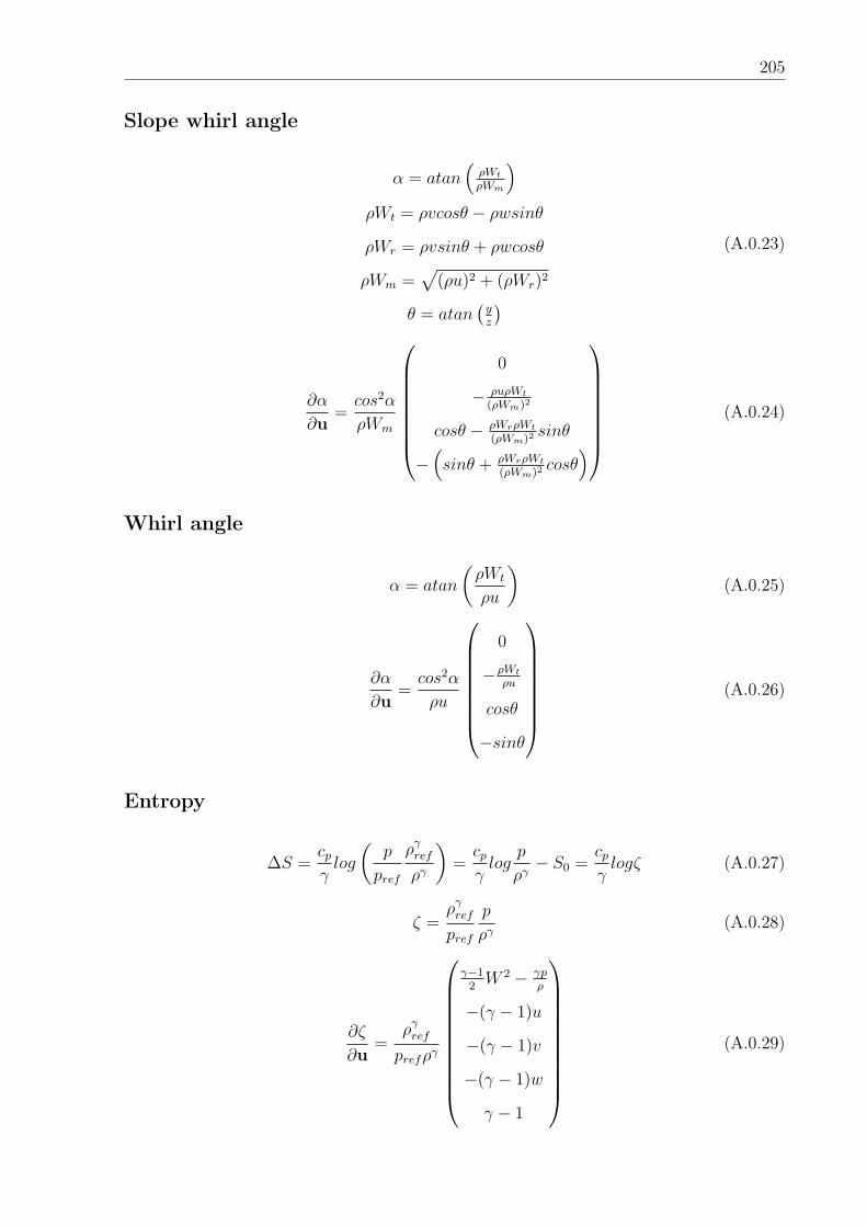
205
Slope whirl angle
α = atan(ρWt
ρWm
)ρWt = ρvcosθ − ρwsinθ
ρWr = ρvsinθ + ρwcosθ
ρWm =√
(ρu)2 + (ρWr)2
θ = atan(yz
)(A.0.23)
∂α
∂u=cos2α
ρWm
0
− ρuρWt
(ρWm)2
cosθ − ρWrρWt
(ρWm)2sinθ
−(sinθ + ρWrρWt
(ρWm)2cosθ
)
(A.0.24)
Whirl angle
α = atan
(ρWt
ρu
)(A.0.25)
∂α
∂u=cos2α
ρu
0
−ρWt
ρu
cosθ
−sinθ
(A.0.26)
Entropy
∆S =cpγlog
(p
pref
ργrefργ
)=cpγlog
p
ργ− S0 =
cpγlogζ (A.0.27)
ζ =ργrefpref
p
ργ(A.0.28)
∂ζ
∂u=
ργrefprefργ
γ−12W 2 − γp
ρ
−(γ − 1)u
−(γ − 1)v
−(γ − 1)w
γ − 1
(A.0.29)
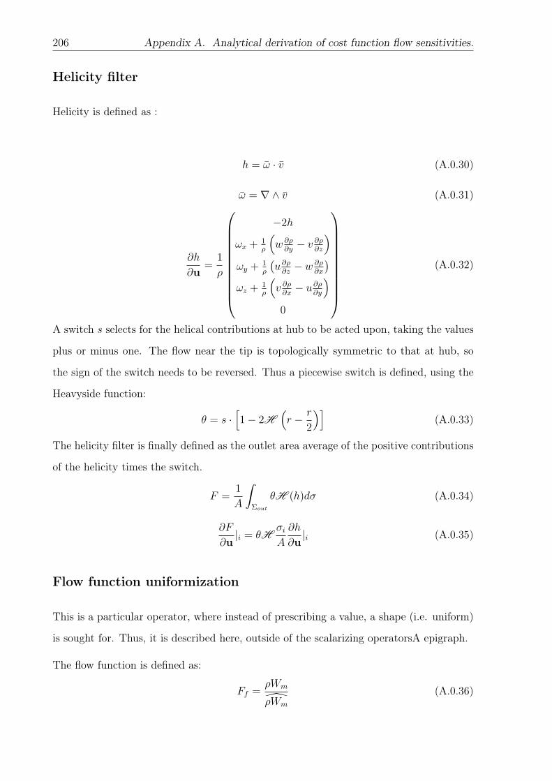
206 Appendix A. Analytical derivation of cost function flow sensitivities.
Helicity filter
Helicity is defined as :
h = ω · v (A.0.30)
ω = ∇∧ v (A.0.31)
∂h
∂u=
1
ρ
−2h
ωx + 1ρ
(w ∂ρ∂y− v ∂ρ
∂z
)ωy + 1
ρ
(u∂ρ∂z− w ∂ρ
∂x
)ωz + 1
ρ
(v ∂ρ∂x− u∂ρ
∂y
)0
(A.0.32)
A switch s selects for the helical contributions at hub to be acted upon, taking the values
plus or minus one. The flow near the tip is topologically symmetric to that at hub, so
the sign of the switch needs to be reversed. Thus a piecewise switch is defined, using the
Heavyside function:
θ = s ·[1− 2H
(r − r
2
)](A.0.33)
The helicity filter is finally defined as the outlet area average of the positive contributions
of the helicity times the switch.
F =1
A
ˆΣout
θH (h)dσ (A.0.34)
∂F
∂u|i = θH
σiA
∂h
∂u|i (A.0.35)
Flow function uniformization
This is a particular operator, where instead of prescribing a value, a shape (i.e. uniform)
is sought for. Thus, it is described here, outside of the scalarizing operatorsA epigraph.
The flow function is defined as:
Ff =ρWm
ρWm
(A.0.36)
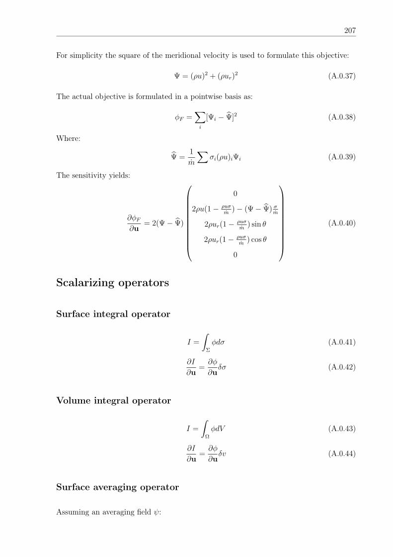
207
For simplicity the square of the meridional velocity is used to formulate this objective:
Ψ = (ρu)2 + (ρur)2 (A.0.37)
The actual objective is formulated in a pointwise basis as:
φF =∑i
[Ψi − Ψ]2 (A.0.38)
Where:
Ψ =1
m
∑σi(ρu)iΨi (A.0.39)
The sensitivity yields:
∂φF∂u
= 2(Ψ− Ψ)
0
2ρu(1− ρuσm
)− (Ψ− Ψ) σm
2ρur(1− ρuσm
) sin θ
2ρur(1− ρuσm
) cos θ
0
(A.0.40)
Scalarizing operators
Surface integral operator
I =
ˆΣ
φdσ (A.0.41)
∂I
∂u=∂φ
∂uδσ (A.0.42)
Volume integral operator
I =
ˆΩ
φdV (A.0.43)
∂I
∂u=∂φ
∂uδv (A.0.44)
Surface averaging operator
Assuming an averaging field ψ:
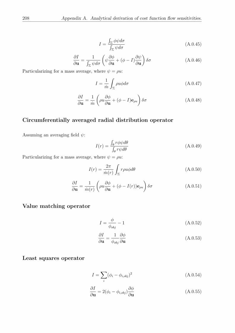
208 Appendix A. Analytical derivation of cost function flow sensitivities.
I =
´Σφψdσ´
Σψdσ
(A.0.45)
∂I
∂u=
1´Σψdσ
(ψ∂φ
∂u+ (φ− I)
∂ψ
∂u
)δσ (A.0.46)
Particularizing for a mass average, where ψ = ρu:
I =1
m
ˆΣ
ρuφdσ (A.0.47)
∂I
∂u=
1
m
(ρu∂φ
∂u+ (φ− I)eρu
)δσ (A.0.48)
Circumferentially averaged radial distribution operator
Assuming an averaging field ψ:
I(r) =
´θrφψdθ´θrψdθ
(A.0.49)
Particularizing for a mass average, where ψ = ρu:
I(r) =2π
m(r)
ˆΣ
rρuφdθ (A.0.50)
∂I
∂u=
1
m(r)
(ρu∂φ
∂u+ (φ− I(r))eρu
)δσ (A.0.51)
Value matching operator
I =φ
φobj− 1 (A.0.52)
∂I
∂u=
1
φobj
∂φ
∂u(A.0.53)
Least squares operator
I =∑i
(φi − φi,obj)2 (A.0.54)
∂I
∂u= 2(φi − φi,obj)
∂φ
∂u(A.0.55)
Appendix B
Adjoint Boundary Conditions.
Non Reflecting Inlet:
At the inlet, stagnation pressure pT , stagnation temperature TT , and tangential and radial
flow angles are imposed. The outgoing Riemann invariant R− is extrapolated from inside
of the computational domain in case of subsonic flow to achieve 1D non reflectivity. In case
of supersonic flow, static pressure is also imposed, with the result that every variable is
determined. Thus, for linearized and adjoint analyses, null Dirichlet boundary conditions
for every variable are applied. The case of subsonic flow is developed in the following.
The outgoing and incoming Riemann invariants are:
R± = Vn ±2c
γ − 1(B.0.1)
Which linearized and applying the perfect gas state equation yield (with subscript 0
denoting the base flow state):
dR± = dVn ±c0
γ − 1(dp
p0
− dρ
ρ0
) (B.0.2)
Combining equation B.0.1 with the definition of total temperature, the following equation
to solve for the static temperature can be derived:
AT +B√T + C = 0 (B.0.3)
209

210 Appendix B. Adjoint Boundary Conditions.
Where the coefficients A, B and C are:
A = 1 + 2(γ−1) cos2 α
B = 2R−√γRg cos2 α
C =R2
−2Cp cos2 α
− TT
(B.0.4)
Linearizing equation B.0.3 yields:
dT
T0
= −(γ − 1)λdR−c0
(B.0.5)
λ =Mn0
Mn0 + cos2 α(B.0.6)
Using isentropic flow relations, we get the static pressure variation:
dp = p0γ
γ − 1
dT
T0
(B.0.7)
and the density variation dρ is obtained via the linearised state equation:
dρ = ρ01
γ − 1
dT
T0
(B.0.8)
Finally, Eq. (B.0.2) provides the new normal velocity:
dvn = dR− +c0
γ − 1
dT
T0
(B.0.9)
To obtain the three components of the velocity we have to multiply the dvn by a
factor depending on the angle of the velocity vector and the normal, thus dV =
[αu αv αw] dVn,inlet, where
αu =cos βs cos βr
cosαn(B.0.10)
αv =sin βs cos θ + cos βs sin βr sin θ
cosαn(B.0.11)
αw =− sin βs sin θ + cos βs sin βr cos θ
cosαn(B.0.12)
βs and βr are the swirl and radial angles at the inlet, and
cosαn = cos βr cos βs · nx + sin βs · ny + sin βr cos βs · nz
θ = arctany
z
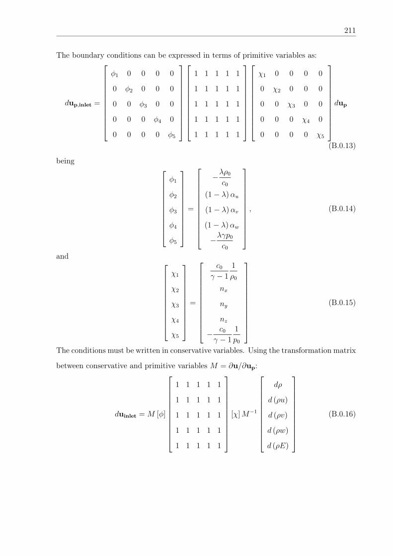
211
The boundary conditions can be expressed in terms of primitive variables as:
dup,inlet =
φ1 0 0 0 0
0 φ2 0 0 0
0 0 φ3 0 0
0 0 0 φ4 0
0 0 0 0 φ5
1 1 1 1 1
1 1 1 1 1
1 1 1 1 1
1 1 1 1 1
1 1 1 1 1
χ1 0 0 0 0
0 χ2 0 0 0
0 0 χ3 0 0
0 0 0 χ4 0
0 0 0 0 χ5
dup
(B.0.13)
being
φ1
φ2
φ3
φ4
φ5
=
−λρ0
c0
(1− λ)αu
(1− λ)αv
(1− λ)αw
−λγp0
c0
, (B.0.14)
and
χ1
χ2
χ3
χ4
χ5
=
c0
γ − 1
1
ρ0
nx
ny
nz
− c0
γ − 1
1
p0
(B.0.15)
The conditions must be written in conservative variables. Using the transformation matrix
between conservative and primitive variables M = ∂u/∂up:
duinlet = M [φ]
1 1 1 1 1
1 1 1 1 1
1 1 1 1 1
1 1 1 1 1
1 1 1 1 1
[χ]M−1
dρ
d (ρu)
d (ρv)
d (ρw)
d (ρE)
(B.0.16)

212 Appendix B. Adjoint Boundary Conditions.
The linearised transposed boundary conditions will then be
vinlet =(M−1
)T[χ]
1 1 1 1 1
1 1 1 1 1
1 1 1 1 1
1 1 1 1 1
1 1 1 1 1
[φ]MTv (B.0.17)
that developed give
vinlet =
χAD1
χAD2
χAD3
χAD4
χAD5
RAD (B.0.18)
being
RAD =
(−λρ0
c0
(v1 + V · v234) + ρ (1− λ)α · v234 −γ
γ − 1
λp0
c0
v5
)(B.0.19)
χAD1
χAD2
χAD3
χAD4
χAD5
=
c0
γ − 1
1
ρ0
(1− (γ − 1)
Vn0
c0
− γ − 1
2
ρ0(u² + v² + w²)2
p0
)nxρ0
+c0u0
p0nyρ0
+c0v0
p0nzρ0
+c0w0
p0
− c0
p0
(B.0.20)
and α = [αu αv αw] .
Non reflecting outlet
At the outlet, for a subsonic condition, static pressure ps is imposed, and the outgoing
Riemmann invariant R+ is extrapolated. For a supersonic outlet, every variable is
extrapolated both for non-linear and linear analyses. Again, the subsonic case is now
expanded.
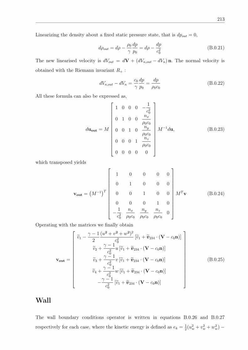
213
Linearizing the density about a fixed static pressure state, that is dpout = 0,
dρout = dρ− ρ0
γ
dp
p0
= dρ− dp
c20
(B.0.21)
The new linearised velocity is dVout = dV + (dVn,out − dVn) n. The normal velocity is
obtained with the Riemann invariant R+ :
dVn,out − dVn =c0
γ
dp
p0
=dp
ρ0c0
(B.0.22)
All these formula can also be expressed as,
duout = M
1 0 0 0 − 1
c20
0 1 0 0nxρ0c0
0 0 1 0nyρ0c0
0 0 0 1nzρ0c0
0 0 0 0 0
M−1du, (B.0.23)
which transposed yields
vout =(M−1
)T
1 0 0 0 0
0 1 0 0 0
0 0 1 0 0
0 0 0 1 0
− 1
c20
nxρ0c0
nyρ0c0
nzρ0c0
0
MTv (B.0.24)
Operating with the matrices we finally obtain
vout =
v1 −γ − 1
2
(u² + v² + w²)2
c20
[v1 + v234 · (V − c0n)]
v2 +γ − 1
c20
u [v1 + v234 · (V − c0n)]
v3 +γ − 1
c20
v [v1 + v234 · (V − c0n)]
v4 +γ − 1
c20
w [v1 + v234 · (V − c0n)]
−γ − 1
c20
[v1 + v234 · (V − c0n)]
(B.0.25)
Wall
The wall boundary conditions operator is written in equations B.0.26 and B.0.27
respectively for each case, where the kinetic energy is defined as ek = 12(u2
w + v2w +w2
w)−
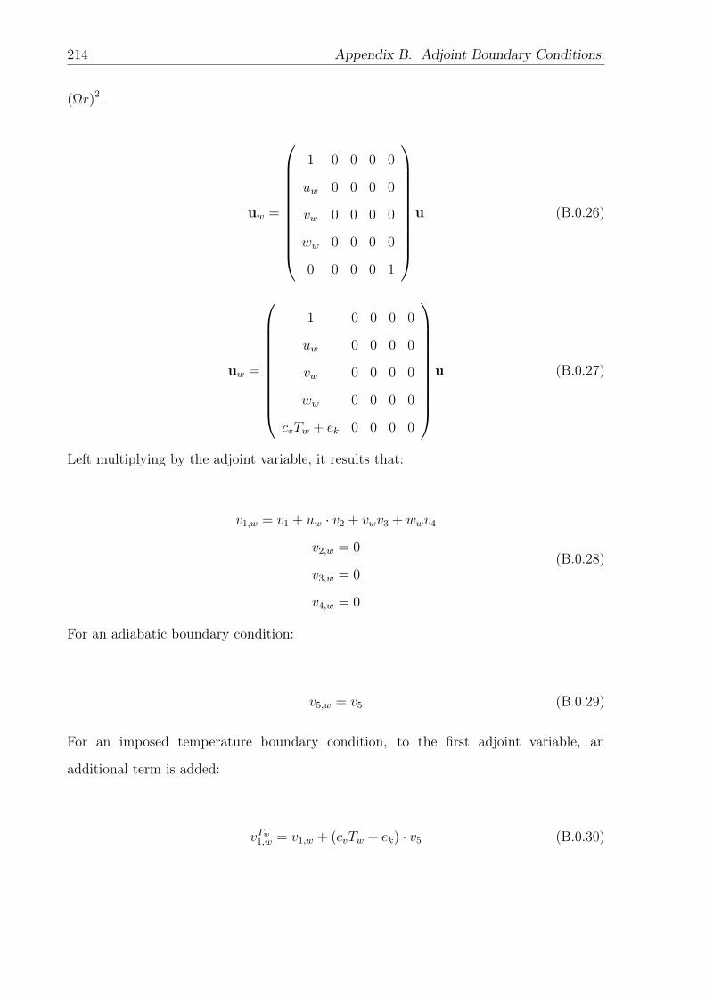
214 Appendix B. Adjoint Boundary Conditions.
(Ωr)2.
uw =
1 0 0 0 0
uw 0 0 0 0
vw 0 0 0 0
ww 0 0 0 0
0 0 0 0 1
u (B.0.26)
uw =
1 0 0 0 0
uw 0 0 0 0
vw 0 0 0 0
ww 0 0 0 0
cvTw + ek 0 0 0 0
u (B.0.27)
Left multiplying by the adjoint variable, it results that:
v1,w = v1 + uw · v2 + vwv3 + wwv4
v2,w = 0
v3,w = 0
v4,w = 0
(B.0.28)
For an adiabatic boundary condition:
v5,w = v5 (B.0.29)
For an imposed temperature boundary condition, to the first adjoint variable, an
additional term is added:
vTw1,w = v1,w + (cvTw + ek) · v5 (B.0.30)

215