automatic control systems - pdhonline.com

www.PDHcenter.com PDH Course E140 www.PDHonline.org

Automatic Control Systems

Part III:

Root Locus Technique

By Shih-Min Hsu, Ph.D., P.E.

of 30


VI. Root Locus Design Method

Since the performance of a closed-loop feedback system can be adjusted by changing one or more parameters, the locations of the roots of the characteristic equation should be evaluated. In the design and analysis of control systems, control engineers often need to investigate a system’s performance when one or more of its parameters vary over a given range. Referring to the transfer function of a typical negative feedback closed-loop system as discussed previously, namely,

( )( )

( )( ) ( )sHsG1

sGsRsC

+= (6-1)

The characteristic equation of the closed-loop system is obtained by setting the

denominator polynomial of the transfer function, ( )( )sR

sC , to zero. Therefore, the roots

of the characteristic equation must satisfy

( ) ( ) 0sHsG1 =+ (6-2)

Let the open-loop transfer function ( ) ( )sHsG express as

( ) ( ) ( )( )

[ ]n1n

1n1

nm1m

1m1

m

asasasbsbsbsK

sDsKNsHsG

++⋅⋅⋅++++⋅⋅⋅++

==−

−−

−

(6-3)

where and are finite polynomials and K is the open-loop gain. Moreover, m is the degree of and n is the degree of

( )sN ( )sD( )sN ( )sD . Equation (6-2) can be replaced as

follows

( )( ) 0sDsKN1 =+ (6-4)

Furthermore, Equation (6-4) can be represented with

( )( ) K

1sDsN

−= (6-5)

The root locus is the locus of values of s for which Equation (6-5) holds for some positive values of K. Namely, if K > 0,

( )( ) K

1sDsN

= (6-6)

and

( )( ) ( ) )180 of multiple odd(or π1k2sDsN

°+=∠ (6-7)

where k=0, ±1, ±2, ±3, ···.

It is worth mentioning that the portion of the root locus when K varies from -∞ to 0 ( ) is called Complementary Root Locus (CRL). For , the portion of Root 0K < 0K >

of 30


Locus is called Direct Root Locus, or simply, Root Locus (RL). This course will only discuss the part that . 0K >

( )sKN

)

s12

+=

) s2 ++

( ) s22Ks++

)( 2s1 +

( )( )sD

sKN=

21 z,z −

If K does not appear as a multiple factor of ( ) ( )sHsG as shown in (6-3), one may need to rearrange the function into the following form:

( ) ( ) 0sDsF =+= (6-8)

Example 6-1: Consider the open-loop transfer function of a control system is

( ) ( ) ( )( )( )2s1ss

5s2K3ssHsG2

+++++

=

Find and in terms of ( )sN (sD ( ) ( ) 0sKNsD =+ . Solution: The characteristic equation of the closed-loop system is

( ) ( ) ( )( )( ) 0

2s1ss5s2K3sHsG1 =

+++++

+

Then,

( )( ( ) ( )( ) 02Ks5s3s2s1ss5s2K32s1ss 2 =++++++=++++

Divide both sides by the terms that do not contain K, namely, ( )( ) 5s3s2s1s 2 +++++s

( ) 053ss1ss

1 2 =+++

+

Therefore,

( ) 2ssN =

and

( ) ( ) 55s4ss53sssssD 232 +++=++++= ♦

The open-loop transfer function of a closed-loop system may sometimes express in terms of the zeros and poles. In this case, Equation (6-3) can be expressed as

( ) ( ) ( )( ) ( )( )( ) ( )n21

m21

pspspszszszsKsHsG

+⋅⋅⋅+++⋅⋅⋅++

= (6-9)

where the zeros ( ) and poles (mz,, −⋅⋅⋅− n21 p,,p,p −⋅⋅⋅−− ) of are real or in complex-conjugate pairs.

( ) ( )sHsG

Example 6-2: For the open-loop transfer function of a given system

( ) ( ) ( )( )( )3s1s

2sKsHsG++

+=

of 30


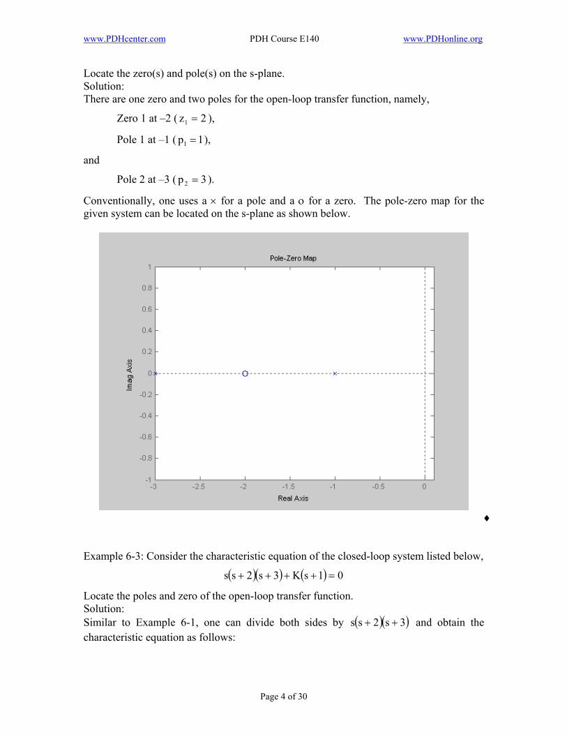
Locate the zero(s) and pole(s) on the s-plane. Solution: There are one zero and two poles for the open-loop transfer function, namely,

Zero 1 at –2 ( ), 2z1 =

Pole 1 at –1 ( p ), 11 =

and

Pole 2 at –3 ( p ). 32 =

Conventionally, one uses a × for a pole and a ο for a zero. The pole-zero map for the given system can be located on the s-plane as shown below.

♦

Example 6-3: Consider the characteristic equation of the closed-loop system listed below,

( )( ) ( ) 01sK3s2ss =++++

Locate the poles and zero of the open-loop transfer function. Solution: Similar to Example 6-1, one can divide both sides by ( )( )3s2ss ++ and obtain the characteristic equation as follows:

of 30


( )( )( ) 0

3s2ss1sK1 =++

++

Therefore, the open-loop transfer function can be obtained,

( ) ( ) ( )( )( )3s2ss

1sKsHsG++

+= .

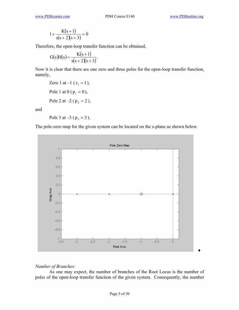
Now it is clear that there are one zero and three poles for the open-loop transfer function, namely,

Zero 1 at –1 ( ), 1z1 =

Pole 1 at 0 ( p ), 01 =

Pole 2 at –2 ( p ), 22 =

and

Pole 3 at –3 ( p ). 33 =

The pole-zero map for the given system can be located on the s-plane as shown below.

♦

Number of Branches: As one may expect, the number of branches of the Root Locus is the number of

poles of the open-loop transfer function of the given system. Consequently, the number

of 30


of branches equals to the order of the polynomial ( )sD , n. All the branches start at poles (K = 0) and approach zeros (K = ∞) of the open-loop transfer function. If there are more poles than zeros ( n ), then, 0m >− mn − branches go to ∞. As mentioned earlier, this course only discusses the Root Locus for . 0>K Root Locus on the Real Axis:

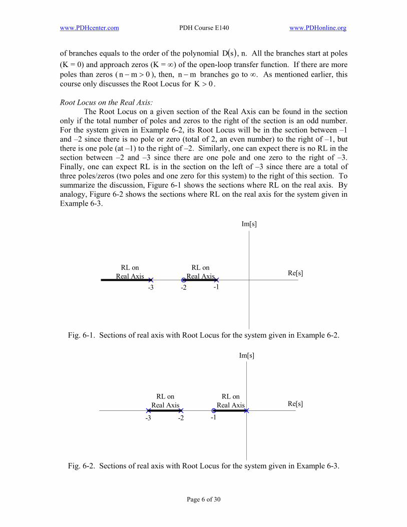
The Root Locus on a given section of the Real Axis can be found in the section only if the total number of poles and zeros to the right of the section is an odd number. For the system given in Example 6-2, its Root Locus will be in the section between –1 and –2 since there is no pole or zero (total of 2, an even number) to the right of –1, but there is one pole (at –1) to the right of –2. Similarly, one can expect there is no RL in the section between –2 and –3 since there are one pole and one zero to the right of –3. Finally, one can expect RL is in the section on the left of –3 since there are a total of three poles/zeros (two poles and one zero for this system) to the right of this section. To summarize the discussion, Figure 6-1 shows the sections where RL on the real axis. By analogy, Figure 6-2 shows the sections where RL on the real axis for the system given in Example 6-3.

-1-2-3

RL onReal Axis

RL onReal Axis Re[s]

Im[s]

Fig. 6-1. Sections of real axis with Root Locus for the system given in Example 6-2.

-1-2-3

RL onReal Axis

RL onReal Axis

Im[s]

Re[s]

Fig. 6-2. Sections of real axis with Root Locus for the system given in Example 6-3.

of 30


Asymptote(s) of Root Locus: The properties of the Root Locus when K → ∞ in the s-plane are important to

know. If n , n – m branches are approaching to infinity in the s-plane when K → ∞. In the other words, for large distances from the origin in the s-plane, the branches of Root Locus approach a set of straight-line asymptotes. For instance, a system with n = 3 (the number of poles) and m = 2 (the number of zeros), then, as K increases, the Root Locus of the two poles would approach to the two zeros while the third pole would approach to the negative infinite of the real axis. In this case, there is only one (

0m >−

1mn ) asymptote. Another instance, a system with n = 2 and m = 0 (2 poles and no zero), as K increases, the root locus of the poles would approach the positive and the negative infinite of the imaginary axis. In this case, there are two (

=−

2mn =− ) asymptotes. These asymptotes from a point in the s-plane on the real axis called the center of asymptotes, or Centroid. The Centroid can be calculated as the sum of poles and zeros divided by n – m, namely,

mn

zp

mnzerospoles

α

m

1ii

n

1ii

−

−−=

−−

=∑∑∑ ∑ == (6-10)

The angle between the asymptotes and the real axis can be calculated as follows:

mn2kππ

A −+

=φ rad, ( )0Kmn,2,1,0,k >−⋅⋅⋅= (6-11)

Example 6-4: What is the Centroid of the system given in Example 6-3? Solution: There are three poles ( ,0p1 = 2p2 = and 3p3 = ) and one zero ( ) for the given system.

1z1 =

( ) ( ) 224

131320α −=−=

−−++

−=

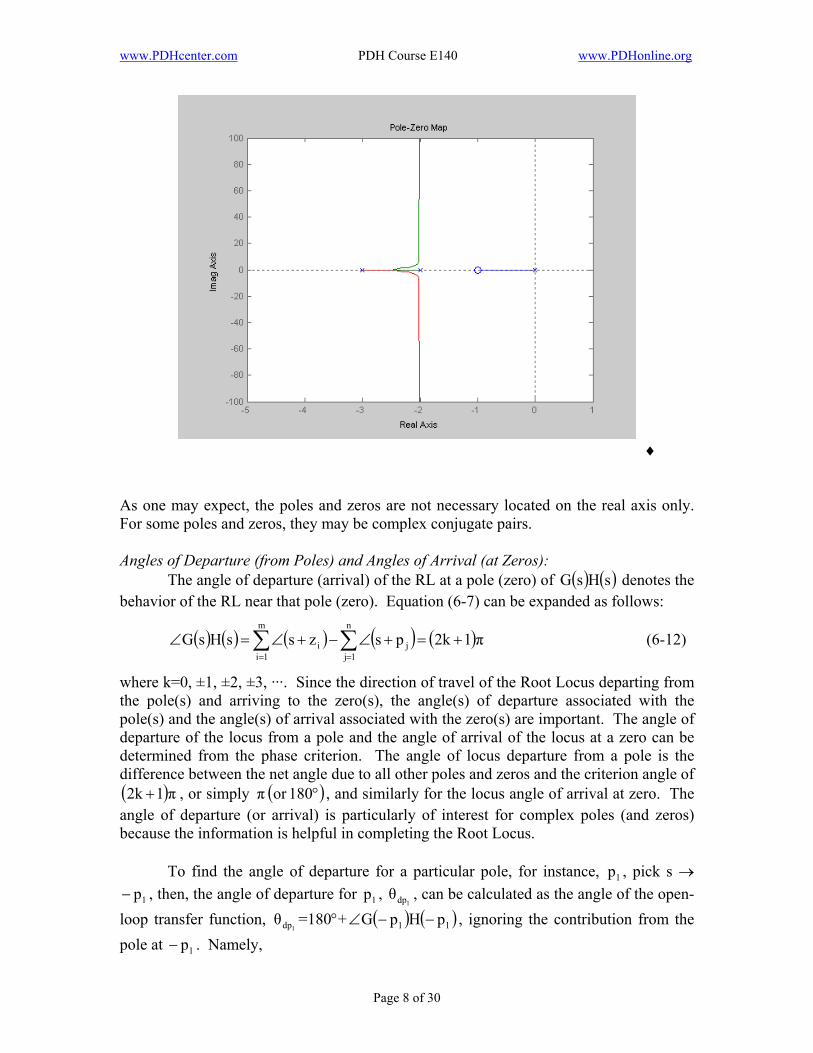
The Root Locus for the given system can be obtained with Matlab as shown below. As one can see clearly, when K increases the pole at 0 approaches to the zero at –1 while the other two poles approach to the two asymptotes with its Centroid at –2. The angles of asymptotes are 2

πand2π − radians, or 90° and –90°, respectively.

of 30


♦ As one may expect, the poles and zeros are not necessary located on the real axis only. For some poles and zeros, they may be complex conjugate pairs. Angles of Departure (from Poles) and Angles of Arrival (at Zeros): The angle of departure (arrival) of the RL at a pole (zero) of denotes the behavior of the RL near that pole (zero). Equation (6-7) can be expanded as follows:

( ) ( )sHsG

( ) ( ) ( ) ( ) ( π12kpszssHsGn

1jj

m

1ii +=+∠−+∠=∠ ∑∑

==

)

) )

(6-12)

where k=0, ±1, ±2, ±3, ···. Since the direction of travel of the Root Locus departing from the pole(s) and arriving to the zero(s), the angle(s) of departure associated with the pole(s) and the angle(s) of arrival associated with the zero(s) are important. The angle of departure of the locus from a pole and the angle of arrival of the locus at a zero can be determined from the phase criterion. The angle of locus departure from a pole is the difference between the net angle due to all other poles and zeros and the criterion angle of

, or simply , and similarly for the locus angle of arrival at zero. The angle of departure (or arrival) is particularly of interest for complex poles (and zeros) because the information is helpful in completing the Root Locus.

( π12k + ( °180orπ

To find the angle of departure for a particular pole, for instance, p , pick s →

, then, the angle of departure for , , can be calculated as the angle of the open-loop transfer function, θ =180°+

1

1p− 1p1dpθ

1dp ( ) ( )1p1 HpG −−∠ , ignoring the contribution from the pole at . Namely, 1p−

of 30


( ) ( ) ( ) ( ) ( )( ) °=+−∠+⋅⋅⋅++−∠+−+−∠+⋅⋅⋅++−∠++−∠ 180ppppθzpzpzp n121dpm12111 1

To find the angle of arrival for a particular zero, for instance, z , pick s → 1 1z− , then, the angle of arrival for , , can be calculated as the angle of the open-loop transfer function, θ =180°–

1z1azθ

1az ( ) ( )11 zHG z −−∠ , ignoring the contribution from 1z− . Namely,

( ) ( ) ( ) ( ) ( )( ) °=+−∠+⋅⋅⋅++−∠++−∠−+−∠+⋅⋅⋅++−∠+ 180pzpzpzzzzzθ n12111m121az1

Example 6-5: Consider a closed-loop system with an open-loop transfer function

( ) ( ) ( )( )( )( )( )2j3s2j3s1s

4j3s4j3sKsHsG++−++

++−+=

which has two zeros at 4j3+− ( )4j3zi.e., 1 −= and 4j3−− ( )4j3zi.e., 2 += , and three poles at , 1− ( ) 3+−1pi.e., 1 = 2j ( )j23pi.e., 2 −= , and 2j3−− ( )2j

2

3pi.e., 3 +=

1z z. Find

the angles of departure for , and p , and the angles of arrival for and . 1p p2 3

Solution: The angle of departure from the pole at 1− ( )1pi.e., 1 = : Since there are three poles and two zeros, the Root Locus would have three branches with two branches starting from two of the complex poles and arriving at the two complex zeros while the pole on the real axis, , approaches to the infinity of the negative Real Axis. Therefore, the angle of departure for is 180°. Or, it could be calculated as follows:

1p

1p

( ) ( ) ( ) ( )( ) °=++−∠+−+−∠+−++−∠+−+−∠ 1802j312j31θ4j314j311dp

( ) ( ) ( ) ( )( ) °=+∠+−∠+−+∠+−∠ 1802j22j2θ4j24j21dp

( )( ) °=°+°−+−°+°− 1804545θ4.634.631dp

°=°−= 180180θ1dp

which gives the same answer.

The angle of departure from the pole at 2j3+− ( )j23pi.e., 2 −= : (( ) ( ) ( ) ( )) °=+++−∠++++−∠−+++−∠+−++−∠ 1802j3j23θ1j234j3j234j3j23

2dp

( ) ( ) ( ) ( )( ) °=∠+++−∠−∠+−∠ 1804jθj226jj22dp

( ) °=°++°−°+°− 18090θ13590902dp

°−=°−=°−°−°−= 4540518090135θ2dp

The angle of departure from the pole at 2j3−− ( )2j3pi.e., 3 += :

(( ) ( ) ( ) ( ) ) °=+−+−−∠++−−∠−++−−∠+−+−−∠ 180θ2j3j231j234j3j234j3j232dp

( ) ( ) ( ) ( )( ) °=+−∠+−−∠−∠+−∠ 180θ4jj222jj63dp

of 30


( ) °=+°−°−−°+°− 180θ9013590903dp

°=°−°+°= 4518090135θ3dp

The angle of arrival to the zero at 4j3+− ( )4j3zi.e., 1 −= :

( ) ( ) ( ) ( )( ) °=+++−∠+−++−∠+++−∠−+++−∠+ 1802j3j432j3j431j434j3j43θ1az

( ) ( ) ( ) ( )( ) °=∠+∠++−∠−∠+ 1806jj2j428jθ1az

°=°=°+°+°+°−°= 6.266.38690906.11690180θ1az

The angle of arrival to the zero at 4j3−− ( )4j3zi.e., 2 += :

( ) ( ) ( ) ( )( ) °=++−−∠+−+−−∠++−−∠−+−+−−∠ 1802j3j432j3j431j43θ4j3j432az

( ) ( ) ( ) ( )( ) °=−∠+−∠+−−∠−+−∠ 1802jj6j42θj82az

( ) ( ) ( ) °−=°−+°−+°−+°+°= 6.2690906.11690180θ2az

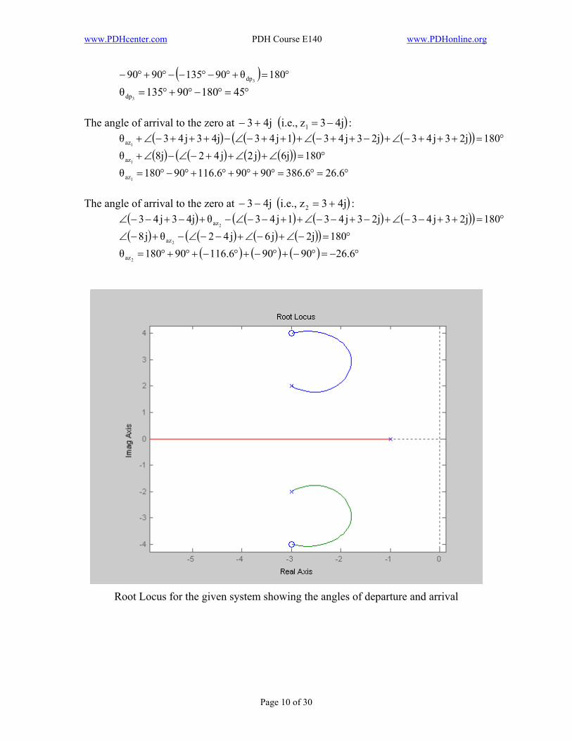
Root Locus for the given system showing the angles of departure and arrival

of 30


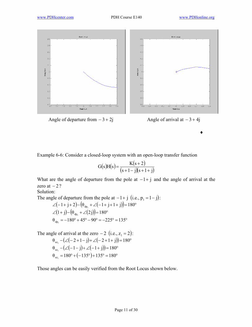
Angle of departure from 2j3+− Angle of arrival at − 4j3+

♦ Example 6-6: Consider a closed-loop system with an open-loop transfer function

( ) ( ) ( )( )( )j1sj1s

2sKsHsG++−+

+=

What are the angle of departure from the pole at j1+− and the angle of arrival at the zero at ? 2−Solution: The angle of departure from the pole at j1+− ( )j1pi.e., 1 −= :

)( ) ( )( °=+++−∠+−++−∠ 180j1j1θ2j11dp

( )( ) ( ) °=∠+−+∠ 180j2θj11dp

°=°−=°−°+°−= 1352259045180θ1dp

The angle of arrival at the zero − 2 ( )2zi.e., 1 = :

( ) ( )( ) °=++−∠+−+−∠− 180j12j12θ1az

( ) ( )( ) °=+−∠+−−∠− 180j1j1θ1az

( )

°=°+°−+°= 180135135180θ1az

Those angles can be easily verified from the Root Locus shown below.

of 30


♦ Crossing of the Imaginary Axis:

As discussed previously, some closed-loop system would be stable only with certain range of K, and that could be determined by Routh-Hurwitz Criterion. Also, when a system is going unstable from a stable region, its Root Locus would intersect with the Imaginary Axis (i.e., Root Locus traveling from the left-half-plane of s-plane to the right-half-plane). The point where the Root Locus intersects/crosses the Imaginary Axis of the s-plane, and the corresponding value of K, may be determined by the means of Routh-Hurwitz Criterion. Example 6-7: Consider a closed-loop system with an open-loop transfer function

( ) ( ) ( )( )22ss3ssKsHsG 2 +++

=

Where the Root Locus intersects the Imaginary Axis and at what K value? Solution: The characteristic equation: ( )( ) 0K6s8s5ssK22ss3ss 2342 =++++=++++

Routh Table

of 30


10

11

212

3

4

sss

65sK81s

dc

bb

8.65

345

61851 ==

×−×=b

K5

01K52 =

×−×=b

6.85K40.8

6.8K566.8

1−

=×−×

=c

K21

211 ==

×= b

cbcd

To have a stable system, and 400K > 0K58. >− . Therefore, . 8.16K0 <<

When K=8.16, the Root Locus intersects the Imaginary Axis which can be obtained from the equation starting with term in the Routh Table, namely,

with K=8.16.

2s0s 2

21 =+ bb

016.8.8s6 2 =+

( )( 0j1.0954sj1.0954s ) =+−

Therefore, the two branches of the Root Locus intersect the following two conjugate points at secrad0954.1± . The Root Locus for the given system is shown below.

of 30


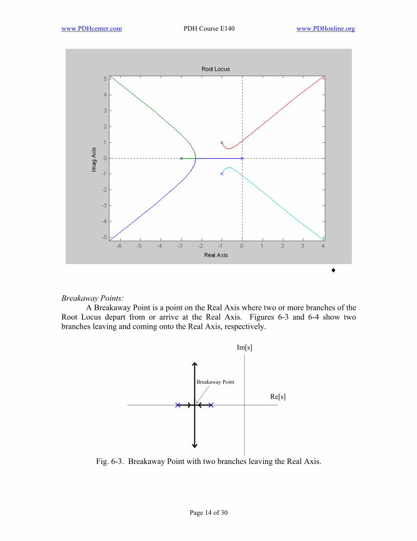
♦ Breakaway Points:

A Breakaway Point is a point on the Real Axis where two or more branches of the Root Locus depart from or arrive at the Real Axis. Figures 6-3 and 6-4 show two branches leaving and coming onto the Real Axis, respectively.

Re[s]

Im[s]

Breakaway Point

Fig. 6-3. Breakaway Point with two branches leaving the Real Axis.

of 30


Re[s]

Im[s]

Breakaway Point

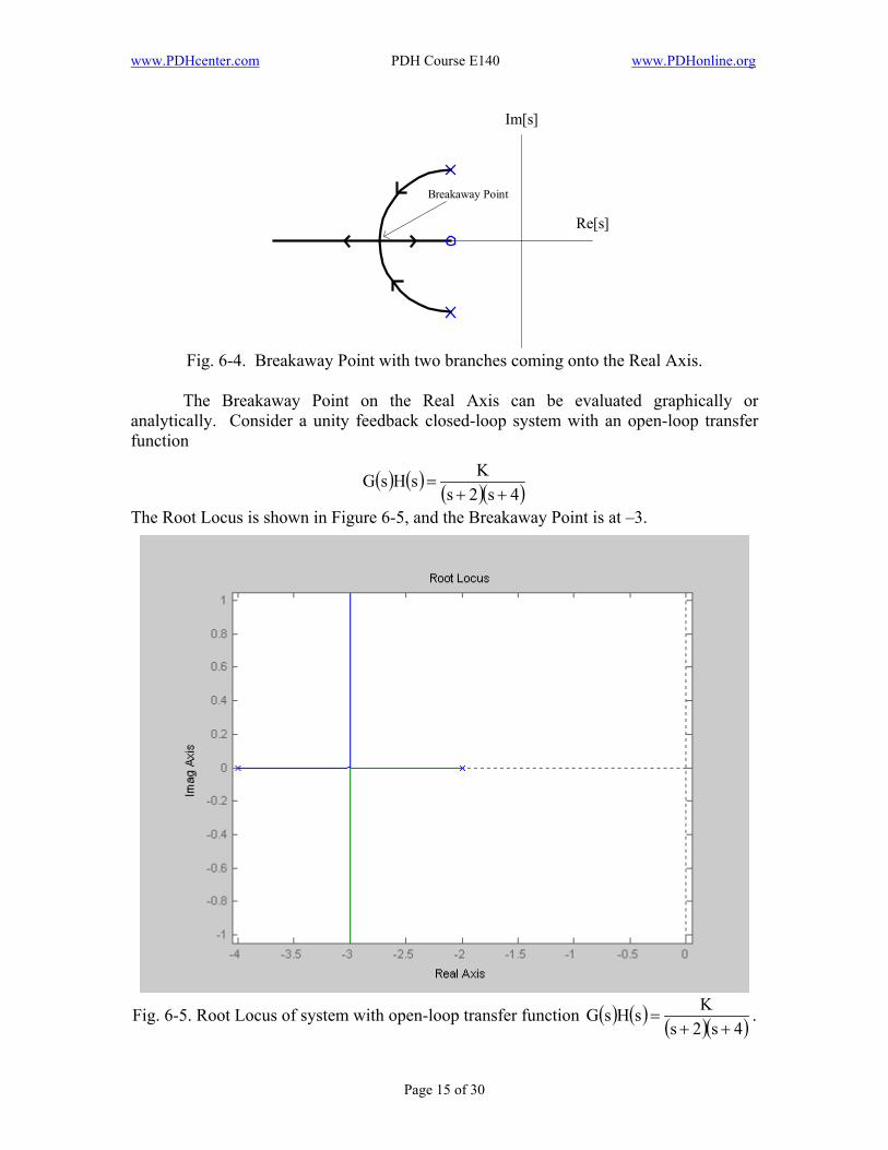
Fig. 6-4. Breakaway Point with two branches coming onto the Real Axis.

The Breakaway Point on the Real Axis can be evaluated graphically or

analytically. Consider a unity feedback closed-loop system with an open-loop transfer function

( ) ( ) ( )( )4s2sKsHsG

++=

The Root Locus is shown in Figure 6-5, and the Breakaway Point is at –3.

Fig. 6-5. Root Locus of system with open-loop transfer function ( ) ( ) ( )( )4s2s

KsHsG++

= .

of 30


The Breakaway Point(s) of the Root Locus of ( ) ( ) ( ) ( ) 0sHsKG1sHsG 11 =1 +=+ , or

( ) ( )sHsG1K

11

−= (6-13)

must satisfy

0dsdK

= (6-14)

For the given system, ( ) ( ) ( )( 4s2ssHsG

1K11

++−=−= ) . Therefore,

( ) ( ) 062sds

86ssddsdK 2

=+−=++

−=

or

3s −= is the Breakaway Point, same as obtained graphically from Figure 6-5.

It is important to point out that the condition for the Breakaway Point given by Equation (6-14) is necessary but not sufficient condition. In other words, all breakaway Point(s) must satisfy Equation (6-14), but not all solutions of Equation (6-14) are Breakaway Points. Example 6-8: For the same system as given in Example 6-7, find the Breakaway Point. Solution:

The open-loop transfer function is ( ) ( ) ( )( )22ss3ssKsHs 2 +++

=G .

Therefore, the K can be expressed as

( ) ( ) ( )( )( )( ) ( )6s8s5ss22ss3ss

22ss3ss1

1G

1K 2342

211

+++−=+++−=

+++

−=−=sHs

( ) 0616s15s4sds

6s8s5ssddsdK 23

234

=+++=+++

=

Therefore, , 2.2886s −= j0.34867307.0s +−= and j0.34867307.0s −−= . However, the Breakaway Point is located only at 2.2886− where the Root Locus on that section of the Real Axis, as shown in the Root Locus for Example 6-7. ♦ Example 6-9: For the same system as given in Example 6-6, find the Breakaway Point. Solution:

of 30


The open-loop transfer function is ( ) ( ) ( )( )( )

( )( )22ss

2sKj1sj1s

2sKsHs 2 +++

=++−+

G += .

Therefore, the K can be expressed as

( ) ( ) ( ) ( )( )

( ) ( )( ) 122

211

2s22ss2s

22ss22ss2s

1sHsG

1K −+++−=+

++−=

+++−=−=

( )( )( ) ( )( ) ( )( ) ( ) 022ss2s12s22sds

2s22ssddsdK 221

12

=+++−+++=+++

= −−−

( )( ) ( )

( )( )( ) ( )

02s

24ss2s

22ss2s22s2s

22ss2s22s

2

2

2

2

2

2

=+

++=

+++−++

=+

++−

++

024ss2 =++

Therefore, and 4142.3s −= 5858.0s −= . However, the Breakaway Point is located only at where the Root Locus on that section of the Real Axis, as shown in the Root Locus for Example 6-6. ♦

4142.3−

Symmetry of the Root Locus:

Another important property of the Root Locus is that a Root Locus is symmetrical with respect to the Real Axis of the s-plane. In general, the Root Locus is symmetrical with respect to the axes of symmetry of the poles and zeros of ( ) ( )sHsG . One should observe such a property from the plots given throughout in this course.

of 30


VII. Guidelines for Sketching a Root Locus The details of the basic properties of the Root Locus of the closed-loop systems have been discussed in the previous section. In this section, a set of step-by-step guidelines for sketching a Root Locus is summarized, and a detailed step-by-step example is presented to illustrate how to use those guidelines to sketch a Root Locus. Rules for the Construction of the Root Locus: 1) Number of Branches: n, where n is the number of poles. 2) Direction of Travel: As ∞→K

0m >, the Root Locus approaches zeros of open-loop

transfer function. If (m is the number of zeros), then, n − mn − branches go to ∞.

3) Root Locus on the Real Axis: If the numbers of poles plus zeros on the right hand

side is an odd number, Root Locus is on the real axis. On the other word, draw Root Locus on the Real Axis to the left of an odd number of poles and zeros.

4) Number of Asymptotes, Angle of Asymptotes and Centroid:

Number of asymptotes: mn −

Angle of asymptote: The angle(s) between the real axis and the asymptote(s) can be calculated as

mn2kππ

A −+

=φ , k ( )0Kmn,0,1,2, >−⋅⋅⋅=

Centroid:

mn

zp

mnzerospoles

α

m

1ii

n

1ii

−

−−=

−−

=∑∑∑ ∑ ==

Table 6-1 shows the angle(s) of asymptote(s) for n 4and32,1,m =− , numerically (in radians) and graphically.

of 30


Table 6-1. Graphical representation of Asymptotes (for n-m =1, 2, 3 & 4).

mn − Aφ Graphical Representation of Asymptotes 1 π

2

2π,

2π

−

3

3ππ,,

3π

− 3π

3π

−

π

4

47π,

45π,

43π,

4π

4π

4π

−

6) Angles of Departure and Angles of Arrival: Angle of departure, :

1dpθ

( ) ( ) ( ) ( ) ( )( ) °=+−∠+⋅⋅⋅++−∠+−+−∠+⋅⋅⋅++−∠++−∠ 180ppppθzpzpzp n121dpm12111 1

Angle of Arrival, θ : 1az

( ) ( ) ( ) ( ) ( )( ) °=+−∠+⋅⋅⋅++−∠++−∠−+−∠+⋅⋅⋅++−∠+ 180pzpzpzzzzzθ n12111m121az1

7) Crossing of the Imaginary Axis: The locations of the Root Locus intersects the

Imaginary Axis can be obtained from the equation starting with s term in the Routh Table, namely, b with K equals the maximum value of the stable range obtained by Routh-Hurwitz Criterion.

2

0s 22

1 =+ b

8) Breakaway Point(s): The breakaway point(s) of the Root Locus of

( ) ( ) ( ) ( ) 0sHsKG1sHsG1 11 =+=+ , or ( ) ( )sHsG1

11

−=K must satisfy 0dsdK

= .

9) Root Locus is symmetry with respect to the Real Axis.

of 30


Example 6-10: A closed-loop negative feedback system has an open-loop transfer function of

( ) ( ) ( )( )136sss

10sKsHsG 2 +++

=

Sketch the Root Locus for K > 0. Solution: There are three poles and one zero, i.e., n=3 and m=1. Therefore, the Root Locus has three branches (n=3), one branch starting from one of the poles and approaching to the zero while the other two branches starting from the two ( n 213m =−=− ) remaining poles and approaching to their Asymptotes ( 2mn =− ) going to infinite when K increases. The poles are located at 0, and j23 +− j23−− while the zero is located at . The Root Locus is on the Real Axis between 0 and

10−10− since the number of pole(s) is an odd

number on the right hand side of the zero at 10− . The angle of Asymptotes can be calculated as follows

mn2kππ

A −+

=φ =

=−==−+

==−

1kfor,2π

23π

132ππ

0kfor,2π

13π

The Centroid can be obtained by

( ) ( )( ) ( ) 213

102j32j30mn

zp

mnzerospoles

α

m

1ii

n

1ii

=−

−++−+−=

−

−−=

−

−=

∑∑∑ ∑ ==

A Centroid with a positive value implies two branches of the Root Locus would travel from the left-half-plane to the right-half-plane of the s-plane. Therefore, those branches would cross the Imaginary Axis and the locations can be obtained as follows:

The characteristic equation: ( ) ( ) ( ) 0K10sK136ss10sK136sss 232 =++++=++++

Routh Table

10

11

2

3

ss

10K6sK131s

cb

+

( )6

K4786

10K1K1361

−=

×−+×=b

K101 =c To have a stable system, and 780K > 0K4 >− . Therefore, 0 . 5.19K <<

of 30


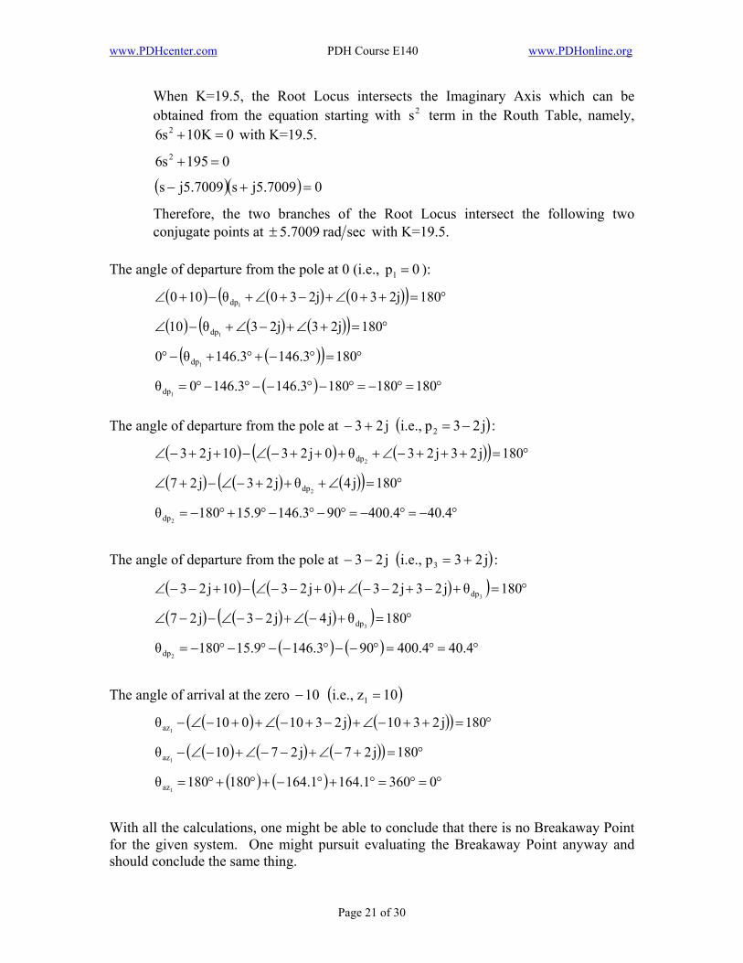
When K=19.5, the Root Locus intersects the Imaginary Axis which can be obtained from the equation starting with term in the Routh Table, namely,

with K=19.5.

2s0K10s6 2 =+

0195s6 2 =+

( )( 0j5.7009sj5.7009s ) =+−

Therefore, the two branches of the Root Locus intersect the following two conjugate points at secrad7009.5± with K=19.5.

The angle of departure from the pole at 0 (i.e., p 01 = ):

( ) ( ) ( )( ) °=++∠+−+∠+−+∠ 1802j302j30θ1001dp

( ) ( ) ( )( ) °=+∠+−∠+−∠ 1802j32j3θ101dp

( )( ) °=°−+°+−° 1803.1463.146θ01dp

( ) °=°−=°−°−−°−°= 1801801803.1463.1460θ1dp

The angle of departure from the pole at j23 +− ( )j23pi.e., 2 −= :

( ) ( ) ( )( ) °=+++−∠++++−∠−++−∠ 180j23j23θ0j2310j232dp

( ) ( ) ( )( ) °=∠+++−∠−+∠ 180j4θj23j272dp

°−=°−=°−°−°+°−= 4.404.400903.1469.15180θ2dp

The angle of departure from the pole at j23 −− ( )j23pi.e., 3 += :

( ) ( ) ( )( ) °=+−+−−∠++−−∠−+−−∠ 180θj23j230j2310j233dp

( ) ( ) ( )( ) °=+−∠+−−∠−−∠ 180θj4j23j273dp

( ) ( ) °=°=°−−°−−°−°−= 4.404.400903.1469.15180θ2dp

The angle of arrival at the zero 10− ( )10zi.e., 1 =

( ) ( ) ( )( ) °=++−∠+−+−∠++−∠− 180j2310j2310010θ1az

( ) ( ) ( )( ) °=+−∠+−−∠+−∠− 180j27j2710θ1az

( ) ( ) °=°=°+°−+°+°= 03601.1641.164180180θ1az

With all the calculations, one might be able to conclude that there is no Breakaway Point for the given system. One might pursuit evaluating the Breakaway Point anyway and should conclude the same thing.

of 30


( )( )

( )( ) ( )( ) 123

2

2

10s13s6ss10s

136sss

136sss10s

1K −+++−=+

++−=

+++

−=

( )( )( ) ( )( ) ( )( ) ( ) 0s316ss01s101s31s123sds

10ss316ssddsdK 23212

123

=+++−++++=+++

= −−−

( )( ) ( )

( )( )( ) ( )

001s

130s201s362s01s

13s6ss01s1312s3s10s

13s6ss10s

1312s3s2

23

2

232

2

232

=+

+++=

+−−−+++

=+

++−

+++

065s6018ss130s201s632s 2323 =+++=+++

Therefore, and sj8632.09691.1s ±−= 0619.14−= . However, there is no Root Locus on the Real Axis at − . So, no Breakaway Point exists as expected. 0619.14

The Root Locus for the given system is sketched below using the information obtained from following the calculations provided in the Guidelines.

-10 -3Re[s]

Im[s]

2

2j

-2j

-3+2j

-3-2j

0

K = 0

K = 0

K = 0

∞→K

∞→K

∞→K

K = 19.5

K = 19.5 5.7009j

-5.7009j

Asymptote 1

Asymptote 2

2π

2π

−

Crossing jω Axis

Crossing jω Axis

Centroid

°− 4.04

°4.04

°180°0

RL on Real Axis

The Root Locus obtained by using MATLAB is shown below to verify the sketched Root Locus.

of 30


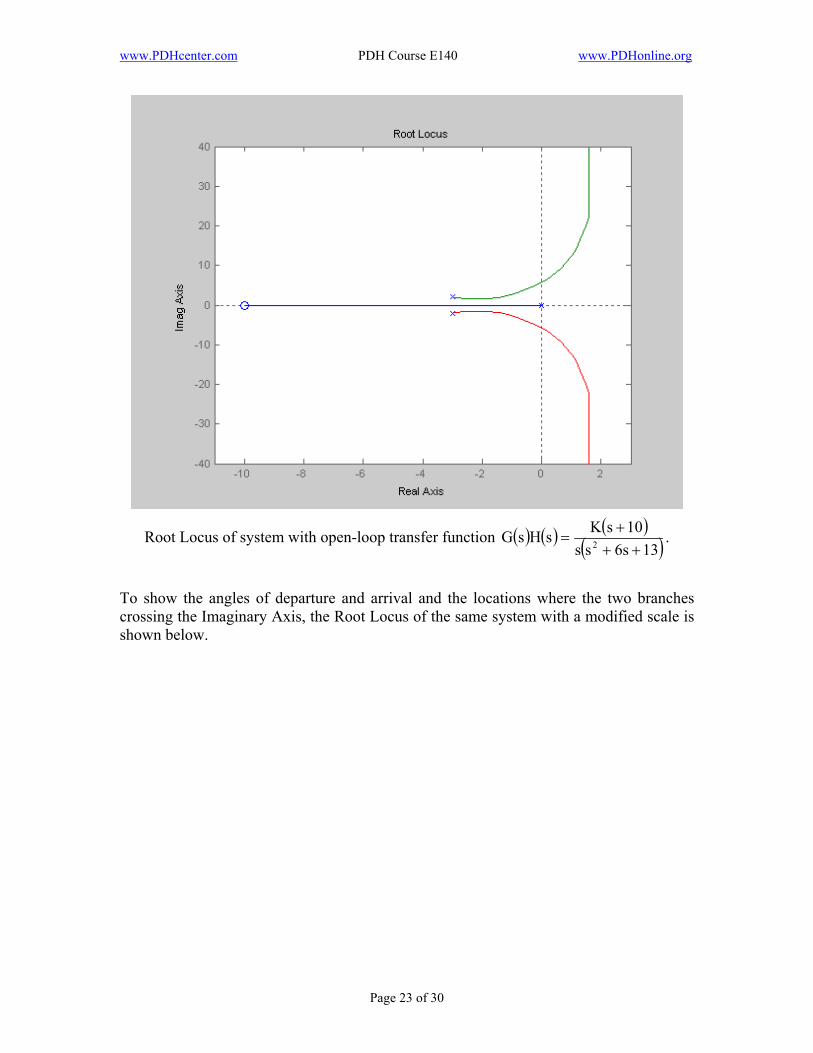
Root Locus of system with open-loop transfer function ( ) ( ) ( )( )136sss

10sKsHs 2 +++

=G .

To show the angles of departure and arrival and the locations where the two branches crossing the Imaginary Axis, the Root Locus of the same system with a modified scale is shown below.

of 30


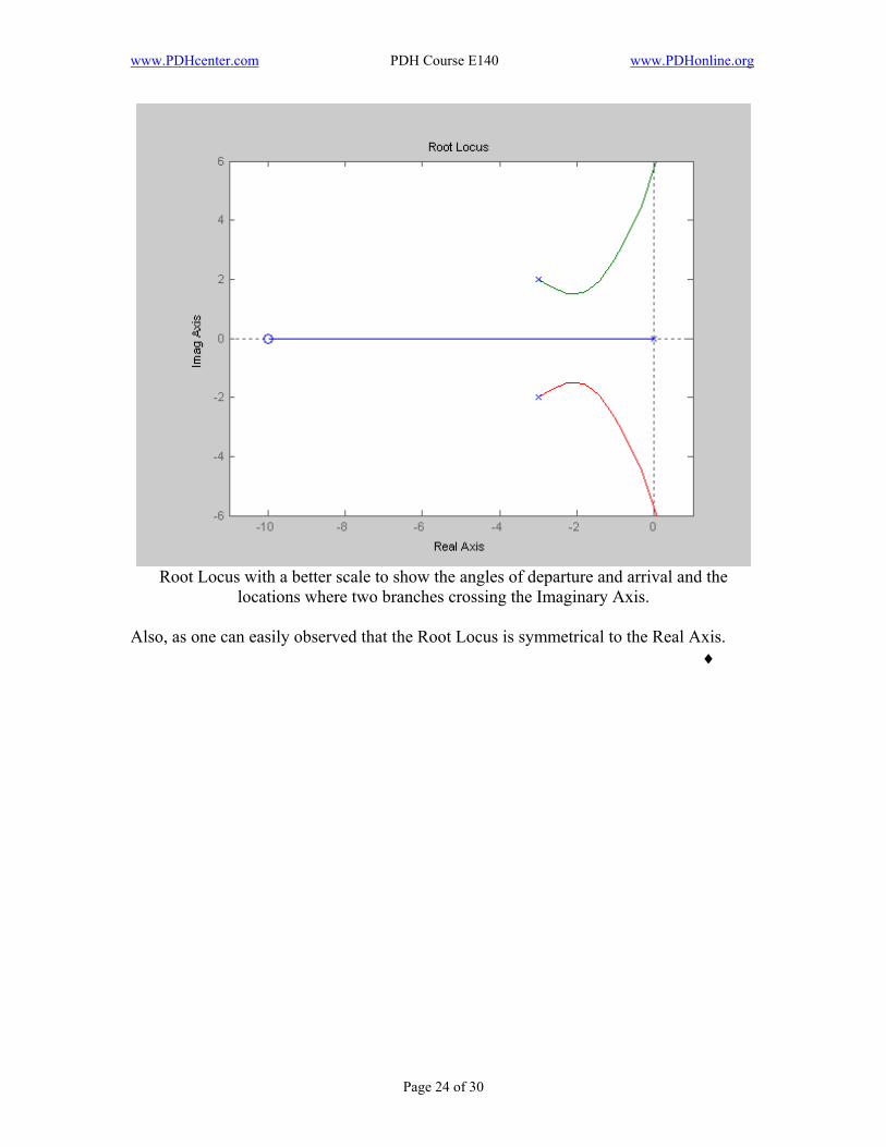
Root Locus with a better scale to show the angles of departure and arrival and the

locations where two branches crossing the Imaginary Axis. Also, as one can easily observed that the Root Locus is symmetrical to the Real Axis. ♦

of 30


References: [1] Gene F. Franklin, J. David Powell and Abbas Emami-Naeini, Feedback Control of

Dynamic Systems – 2nd Edition, Addison Wesley, 1991 [2] Benjamin C. Kuo, Automatic Control Systems – 5th Edition, Prentice-Hall, 1987 [3] Richard C. Dorf, Modern Control Systems – 6th Edition, Addison Wesley, 1992 [4] John A. Camara, Practice Problems for the Electrical and Computer Engineering

PE Exam – 6th Edition, Professional Publications, 2002 [5] NCEES, Fundamentals of Engineering Supplied-Reference Handbook – 6th Edition,

2003 [6] Merle C. Potter, FE/EIT Electrical Discipline-Specific Review for the FE/EIT Exam

– 5th Edition, Great Lakes Press, 2001 [7] Merle C. Potter, Principles & Practice of Electrical Engineering – 1st Edition, Great

Lakes Press, 1998 [8] Joseph J. DiStefano, III, Allen R. Stubberud, and Ivan J. Williams, Feedback and

Control Systems – 2nd Edition, McGraw-Hill, 1990

of 30


Appendix A How to use MATLAB to obtain the Root Locus

Example 6-5: >> num=[1 6 25]; >> den=[1 7 19 13]; >> [z,p,k]=tf2zp(num,den); >> z z = -3.0000 + 4.0000i -3.0000 - 4.0000i >> P p = -3.0000 + 2.0000i -3.0000 - 2.0000i -1.0000 >> pzmap(p,z)

of 30


>> rlocus(num,den)

To change scale of the Real Axis and Imaginary Axis to show the angles of departure and arrival >> v=[-3.5 –2.5 1.5 2.5]; >> axis(v)

of 30


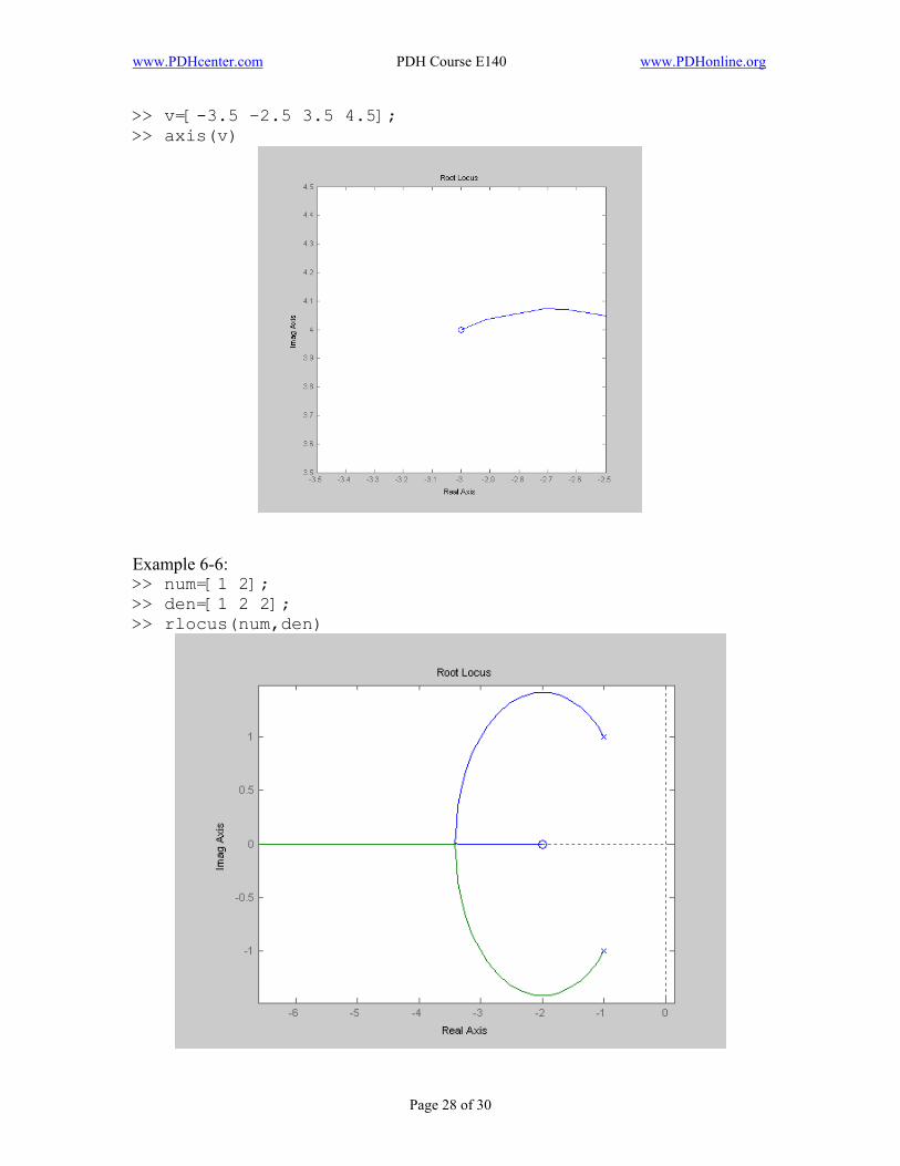
>> v=[-3.5 –2.5 3.5 4.5]; >> axis(v)

Example 6-6: >> num=[1 2]; >> den=[1 2 2]; >> rlocus(num,den)

of 30


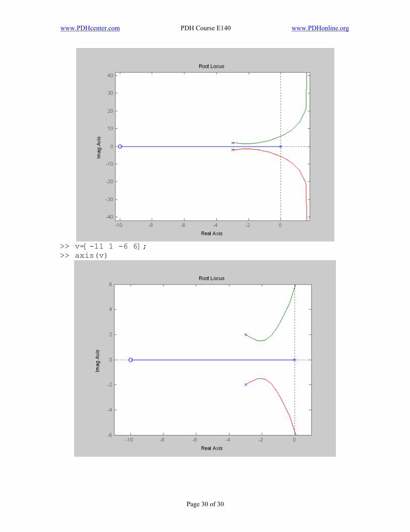
Example 6-10: >> num=[1 10]; >> den=[1 6 13 0]; >> [p,z]=pzmap(num,den) p = 0 -3.0000 + 2.0000i -3.0000 - 2.0000i z = -10 >> pzmap(p,z) >> v=[-11 1 -6 6]; >> axis(v)

>> rlocus(num,den)

of 30


>> v=[-11 1 -6 6]; >> axis(v)

of 30

automatic control systems - pdhonline.com

Documents