automated landscape painting in the style of bob ross
TRANSCRIPT

Automated Landscape Painting
in the Style of
Bob Ross
by
Alex Kalaidjian
A thesis
presented to the University of Waterloo
in fulfillment of the
thesis requirement for the degree of
Master of Mathematics
in
Computer Science
Waterloo, Ontario, Canada, 2007
c© Alex Kalaidjian 2007


I hereby declare that I am the sole author of this thesis. This is a true copy of the thesis,
including any required final revisions, as accepted by my examiners.
I understand that my thesis may be made electronically available to the public.
iii

Abstract
This thesis presents a way of automatically generating a landscape painting in the artis-
tic style of Bob Ross. First, a relatively simple, yet effective and versatile, painting model
is presented. The brushes of the painting model can be used on their own for creative appli-
cations or as a lower layer to the software components responsible for automation. Next,
the brush strokes and parameters used to automatically paint eight different landscape
features, each with its own adjustable attributes and randomized forms, are described.
Finally, the placement of all of the automated landscape features required to achieve the
layout of one of Bob Ross’s landscape paintings is shown.
v


Acknowledgements
I would like to thank my supervisors Stephen Mann and Craig Kaplan for their guidance
and sense of humour. Steve, you were an excellent mentor throughout my studies and your
sense of reasoning through experience along with your ice cream creation skills was greatly
appreciated. Craig, thank you for thinking of and helping me pursue a topic for my thesis
that was fun, highly presentable, and that my parents could understand. I would also
like to thank my readers Bill Cowan and Doug Kirton for their helpful comments and
suggestions. Although I only realised it toward the end, the members of the CGL, new
and old, are always there, waiting for you to embrace their willingness to help or go have
a drink after a long day of work. Finally, thank you to my family for their unconditional
support.
This research was funded by scholarships from the Natural Sciences and Engineering
Research Council of Canada (NSERC) and the University of Waterloo.
vii


Contents
List of Tables xvii
List of Figures xix
1 Introduction 1
1.1 Bob Ross . . . . . . . . . . . . . . . . . . . . . . . . . . . . . . . . . . . . 2
1.2 Objectives . . . . . . . . . . . . . . . . . . . . . . . . . . . . . . . . . . . . 3
1.3 Contributions . . . . . . . . . . . . . . . . . . . . . . . . . . . . . . . . . . 4
1.4 Outline . . . . . . . . . . . . . . . . . . . . . . . . . . . . . . . . . . . . . . 5
2 Background 7
2.1 Previous Work . . . . . . . . . . . . . . . . . . . . . . . . . . . . . . . . . 7
2.1.1 Painting Models . . . . . . . . . . . . . . . . . . . . . . . . . . . . . 8
2.1.2 Painterly Rendering . . . . . . . . . . . . . . . . . . . . . . . . . . 9
2.2 Commercial Applications . . . . . . . . . . . . . . . . . . . . . . . . . . . . 10
3 Application and Canvas 13
3.1 Architecture . . . . . . . . . . . . . . . . . . . . . . . . . . . . . . . . . . . 13
3.2 Canvas . . . . . . . . . . . . . . . . . . . . . . . . . . . . . . . . . . . . . . 14
3.2.1 Factors Influencing Design . . . . . . . . . . . . . . . . . . . . . . . 15
3.2.2 Design . . . . . . . . . . . . . . . . . . . . . . . . . . . . . . . . . . 15
ix
3.3 Undo and Redo . . . . . . . . . . . . . . . . . . . . . . . . . . . . . . . . . 17
3.3.1 Simple Method . . . . . . . . . . . . . . . . . . . . . . . . . . . . . 18
3.3.2 Improved Method . . . . . . . . . . . . . . . . . . . . . . . . . . . . 18
3.4 User Interface . . . . . . . . . . . . . . . . . . . . . . . . . . . . . . . . . . 18
3.4.1 Painting Modes . . . . . . . . . . . . . . . . . . . . . . . . . . . . . 19
3.4.2 Options and Controls . . . . . . . . . . . . . . . . . . . . . . . . . . 19
3.4.3 Learning How To Paint Like Bob Ross . . . . . . . . . . . . . . . . 20
4 Brushes 21
4.1 Requirements . . . . . . . . . . . . . . . . . . . . . . . . . . . . . . . . . . 22
4.1.1 Different Kinds of Brushes . . . . . . . . . . . . . . . . . . . . . . . 22
4.1.2 General Operations . . . . . . . . . . . . . . . . . . . . . . . . . . . 23
4.1.3 Blending . . . . . . . . . . . . . . . . . . . . . . . . . . . . . . . . . 23
4.2 Painting Entities . . . . . . . . . . . . . . . . . . . . . . . . . . . . . . . . 24
4.2.1 Paint Amount and Colour . . . . . . . . . . . . . . . . . . . . . . . 24
4.2.2 A Drop of Paint . . . . . . . . . . . . . . . . . . . . . . . . . . . . . 25
4.2.3 Alpha Blending . . . . . . . . . . . . . . . . . . . . . . . . . . . . . 26
4.2.4 Paint Loss . . . . . . . . . . . . . . . . . . . . . . . . . . . . . . . . 27
4.2.5 Painting States . . . . . . . . . . . . . . . . . . . . . . . . . . . . . 27
4.2.6 Paint Blending . . . . . . . . . . . . . . . . . . . . . . . . . . . . . 29
4.2.7 3D Effect . . . . . . . . . . . . . . . . . . . . . . . . . . . . . . . . 34
4.3 General Brush Operations and Attributes . . . . . . . . . . . . . . . . . . . 35
4.3.1 Painting Entity Locations . . . . . . . . . . . . . . . . . . . . . . . 35
4.3.2 Brush Orientation . . . . . . . . . . . . . . . . . . . . . . . . . . . . 36
4.3.3 Paint Loading . . . . . . . . . . . . . . . . . . . . . . . . . . . . . . 36
4.3.4 Alternate Painting Modes . . . . . . . . . . . . . . . . . . . . . . . 37
4.3.5 Strokes . . . . . . . . . . . . . . . . . . . . . . . . . . . . . . . . . . 38
4.4 One and Two Inch Brushes . . . . . . . . . . . . . . . . . . . . . . . . . . 39
4.5 Round Brush . . . . . . . . . . . . . . . . . . . . . . . . . . . . . . . . . . 42
x
4.6 Fan Brush . . . . . . . . . . . . . . . . . . . . . . . . . . . . . . . . . . . . 43
4.6.1 Symmetric Footprint . . . . . . . . . . . . . . . . . . . . . . . . . . 43
4.6.2 Corner Footprint . . . . . . . . . . . . . . . . . . . . . . . . . . . . 46
4.6.3 Painting Entity Placement . . . . . . . . . . . . . . . . . . . . . . . 47
4.7 Filbert Brush . . . . . . . . . . . . . . . . . . . . . . . . . . . . . . . . . . 47
4.8 Liner Brush . . . . . . . . . . . . . . . . . . . . . . . . . . . . . . . . . . . 48
4.9 Palette Knife . . . . . . . . . . . . . . . . . . . . . . . . . . . . . . . . . . 49
4.9.1 Painting Entity Alterations . . . . . . . . . . . . . . . . . . . . . . 49
4.9.2 Painting Entity Locations . . . . . . . . . . . . . . . . . . . . . . . 52
4.9.3 Paint Breaks . . . . . . . . . . . . . . . . . . . . . . . . . . . . . . 52
4.9.4 Scratching the Canvas . . . . . . . . . . . . . . . . . . . . . . . . . 56
4.9.5 More Examples . . . . . . . . . . . . . . . . . . . . . . . . . . . . . 56
4.10 Conservation of Paint . . . . . . . . . . . . . . . . . . . . . . . . . . . . . . 58
4.11 Paintings . . . . . . . . . . . . . . . . . . . . . . . . . . . . . . . . . . . . . 58
5 Landscape Features 59
5.1 Painting Process . . . . . . . . . . . . . . . . . . . . . . . . . . . . . . . . 60
5.2 Reference Point . . . . . . . . . . . . . . . . . . . . . . . . . . . . . . . . . 60
5.3 Brush Strokes . . . . . . . . . . . . . . . . . . . . . . . . . . . . . . . . . . 61
5.3.1 Parabolic Stroke . . . . . . . . . . . . . . . . . . . . . . . . . . . . 61
5.3.2 Criss-Cross Stroke . . . . . . . . . . . . . . . . . . . . . . . . . . . 62
5.3.3 Bezier Curve Stroke . . . . . . . . . . . . . . . . . . . . . . . . . . . 63
5.3.4 Jagged Strokes . . . . . . . . . . . . . . . . . . . . . . . . . . . . . 63
5.3.5 Randomness . . . . . . . . . . . . . . . . . . . . . . . . . . . . . . . 64
5.4 Forest Hills . . . . . . . . . . . . . . . . . . . . . . . . . . . . . . . . . . . 65
5.5 Mountain Feature . . . . . . . . . . . . . . . . . . . . . . . . . . . . . . . . 65
5.5.1 Undercoat . . . . . . . . . . . . . . . . . . . . . . . . . . . . . . . . 66
5.5.2 Undercoat Blending . . . . . . . . . . . . . . . . . . . . . . . . . . . 67
5.5.3 Ledges . . . . . . . . . . . . . . . . . . . . . . . . . . . . . . . . . . 69
xi
5.5.4 Snow Paint Order . . . . . . . . . . . . . . . . . . . . . . . . . . . . 69
5.5.5 Snow Shadows . . . . . . . . . . . . . . . . . . . . . . . . . . . . . . 70
5.5.6 Illuminated Snow . . . . . . . . . . . . . . . . . . . . . . . . . . . . 71
5.5.7 Snow Blending . . . . . . . . . . . . . . . . . . . . . . . . . . . . . 72
5.5.8 Adjustable Attributes . . . . . . . . . . . . . . . . . . . . . . . . . 74
5.6 Other Features . . . . . . . . . . . . . . . . . . . . . . . . . . . . . . . . . 74
6 Landscape Layout 79
6.1 Sky Placement . . . . . . . . . . . . . . . . . . . . . . . . . . . . . . . . . 80
6.2 Mountain Placement . . . . . . . . . . . . . . . . . . . . . . . . . . . . . . 82
6.3 Lake Placement . . . . . . . . . . . . . . . . . . . . . . . . . . . . . . . . . 83
6.4 Hills Placement . . . . . . . . . . . . . . . . . . . . . . . . . . . . . . . . . 83
6.5 Evergreen Tree Placement . . . . . . . . . . . . . . . . . . . . . . . . . . . 86
6.5.1 On Deciduous Trees Side . . . . . . . . . . . . . . . . . . . . . . . . 87
6.5.2 On Non-Deciduous Trees Side . . . . . . . . . . . . . . . . . . . . . 87
6.6 Deciduous Tree Placement . . . . . . . . . . . . . . . . . . . . . . . . . . . 89
6.7 Rocky Bank Placement . . . . . . . . . . . . . . . . . . . . . . . . . . . . . 90
6.7.1 On Deciduous Tree Side . . . . . . . . . . . . . . . . . . . . . . . . 90
6.7.2 On Non-Deciduous Tree Side . . . . . . . . . . . . . . . . . . . . . 92
6.8 Bush Placement . . . . . . . . . . . . . . . . . . . . . . . . . . . . . . . . . 92
6.8.1 On Deciduous Tree Side . . . . . . . . . . . . . . . . . . . . . . . . 94
6.8.2 On Non-Deciduous Tree Side . . . . . . . . . . . . . . . . . . . . . 95
6.9 Other Paintings . . . . . . . . . . . . . . . . . . . . . . . . . . . . . . . . . 96
7 Conclusion 99
7.1 Results . . . . . . . . . . . . . . . . . . . . . . . . . . . . . . . . . . . . . . 99
7.1.1 Painting Model . . . . . . . . . . . . . . . . . . . . . . . . . . . . . 100
7.1.2 Landscape Features . . . . . . . . . . . . . . . . . . . . . . . . . . . 101
7.1.3 Landscape Layout . . . . . . . . . . . . . . . . . . . . . . . . . . . . 101
xii
7.1.4 User Interface . . . . . . . . . . . . . . . . . . . . . . . . . . . . . . 101
7.2 Critique . . . . . . . . . . . . . . . . . . . . . . . . . . . . . . . . . . . . . 102
7.2.1 Automating the Painting of Another Landscape . . . . . . . . . . . 102
7.2.2 Automating the Painting of Another Landscape Feature . . . . . . 105
7.2.3 Comparison of my Automated Painting to the Real Thing . . . . . 106
7.3 Limitations . . . . . . . . . . . . . . . . . . . . . . . . . . . . . . . . . . . 108
7.4 Future Work . . . . . . . . . . . . . . . . . . . . . . . . . . . . . . . . . . . 109
A Landscape Feature Details 111
A.1 Sky Feature . . . . . . . . . . . . . . . . . . . . . . . . . . . . . . . . . . . 111
A.1.1 Sunny Area . . . . . . . . . . . . . . . . . . . . . . . . . . . . . . . 111
A.1.2 Clouds . . . . . . . . . . . . . . . . . . . . . . . . . . . . . . . . . . 113
A.1.3 Blending . . . . . . . . . . . . . . . . . . . . . . . . . . . . . . . . . 116
A.1.4 Adjustable Attributes . . . . . . . . . . . . . . . . . . . . . . . . . 117
A.2 Lake Feature . . . . . . . . . . . . . . . . . . . . . . . . . . . . . . . . . . 117
A.2.1 Sunny Reflection . . . . . . . . . . . . . . . . . . . . . . . . . . . . 118
A.2.2 Surrounding Area . . . . . . . . . . . . . . . . . . . . . . . . . . . . 119
A.2.3 Blending . . . . . . . . . . . . . . . . . . . . . . . . . . . . . . . . . 119
A.2.4 Adjustable Attributes . . . . . . . . . . . . . . . . . . . . . . . . . 120
A.3 Hills Feature . . . . . . . . . . . . . . . . . . . . . . . . . . . . . . . . . . . 121
A.3.1 Shapes . . . . . . . . . . . . . . . . . . . . . . . . . . . . . . . . . . 121
A.3.2 Undercoat . . . . . . . . . . . . . . . . . . . . . . . . . . . . . . . . 123
A.3.3 Highlights . . . . . . . . . . . . . . . . . . . . . . . . . . . . . . . . 124
A.3.4 Mist . . . . . . . . . . . . . . . . . . . . . . . . . . . . . . . . . . . 125
A.3.5 Reflections . . . . . . . . . . . . . . . . . . . . . . . . . . . . . . . . 126
A.3.6 Water Ripples . . . . . . . . . . . . . . . . . . . . . . . . . . . . . . 128
A.3.7 Adjustable Attributes . . . . . . . . . . . . . . . . . . . . . . . . . 130
A.4 Evergreen Tree Feature . . . . . . . . . . . . . . . . . . . . . . . . . . . . . 131
A.4.1 Leaf Stab Locations . . . . . . . . . . . . . . . . . . . . . . . . . . . 131
xiii

A.4.2 Undercoat . . . . . . . . . . . . . . . . . . . . . . . . . . . . . . . . 133
A.4.3 Trunk . . . . . . . . . . . . . . . . . . . . . . . . . . . . . . . . . . 134
A.4.4 Leaves Covering the Trunk . . . . . . . . . . . . . . . . . . . . . . . 135
A.4.5 Highlights . . . . . . . . . . . . . . . . . . . . . . . . . . . . . . . . 136
A.4.6 Reflection . . . . . . . . . . . . . . . . . . . . . . . . . . . . . . . . 136
A.4.7 Adjustable Attributes . . . . . . . . . . . . . . . . . . . . . . . . . 138
A.5 Deciduous Tree Feature . . . . . . . . . . . . . . . . . . . . . . . . . . . . . 142
A.5.1 Trunk . . . . . . . . . . . . . . . . . . . . . . . . . . . . . . . . . . 143
A.5.2 Branches . . . . . . . . . . . . . . . . . . . . . . . . . . . . . . . . . 145
A.5.3 Leaves . . . . . . . . . . . . . . . . . . . . . . . . . . . . . . . . . . 147
A.5.4 Adjustable Attributes . . . . . . . . . . . . . . . . . . . . . . . . . 150
A.6 Rocky Bank Feature . . . . . . . . . . . . . . . . . . . . . . . . . . . . . . 153
A.6.1 Strokes . . . . . . . . . . . . . . . . . . . . . . . . . . . . . . . . . . 153
A.6.2 Undercoat . . . . . . . . . . . . . . . . . . . . . . . . . . . . . . . . 154
A.6.3 Reflection . . . . . . . . . . . . . . . . . . . . . . . . . . . . . . . . 155
A.6.4 Bottom Texture . . . . . . . . . . . . . . . . . . . . . . . . . . . . . 156
A.6.5 Top Surface . . . . . . . . . . . . . . . . . . . . . . . . . . . . . . . 157
A.6.6 Top Surface Highlights . . . . . . . . . . . . . . . . . . . . . . . . . 157
A.6.7 Water Ripples . . . . . . . . . . . . . . . . . . . . . . . . . . . . . . 158
A.6.8 Rock Layout . . . . . . . . . . . . . . . . . . . . . . . . . . . . . . . 159
A.6.9 Another Small Rock on Top . . . . . . . . . . . . . . . . . . . . . . 159
A.6.10 Adjustable Attributes . . . . . . . . . . . . . . . . . . . . . . . . . 159
A.7 Bush Feature . . . . . . . . . . . . . . . . . . . . . . . . . . . . . . . . . . 161
A.7.1 Leaf Locations . . . . . . . . . . . . . . . . . . . . . . . . . . . . . 161
A.7.2 Undercoat . . . . . . . . . . . . . . . . . . . . . . . . . . . . . . . . 162
A.7.3 Branches . . . . . . . . . . . . . . . . . . . . . . . . . . . . . . . . . 162
A.7.4 Leaves Covering Branches . . . . . . . . . . . . . . . . . . . . . . . 163
A.7.5 Highlights . . . . . . . . . . . . . . . . . . . . . . . . . . . . . . . . 164
xiv

A.7.6 Adjustable Attributes . . . . . . . . . . . . . . . . . . . . . . . . . 165
B Feature Paint Colours 169
C Additional Paintings 173
Bibliography 179
xv


List of Tables
5.1 Other feature figures and appendix sections . . . . . . . . . . . . . . . . . 75
6.1 Evergreen tree locations on the non-deciduous trees side . . . . . . . . . . 88
B.1 Sky colours . . . . . . . . . . . . . . . . . . . . . . . . . . . . . . . . . . . 169
B.2 Mountain colours . . . . . . . . . . . . . . . . . . . . . . . . . . . . . . . . 169
B.3 Lake colours . . . . . . . . . . . . . . . . . . . . . . . . . . . . . . . . . . . 170
B.4 Hills colours . . . . . . . . . . . . . . . . . . . . . . . . . . . . . . . . . . . 170
B.5 Evergreen tree colours . . . . . . . . . . . . . . . . . . . . . . . . . . . . . 170
B.6 Deciduous tree colours . . . . . . . . . . . . . . . . . . . . . . . . . . . . . 170
B.7 Rocky bank colours . . . . . . . . . . . . . . . . . . . . . . . . . . . . . . . 171
B.8 Bush colours . . . . . . . . . . . . . . . . . . . . . . . . . . . . . . . . . . . 171
xvii

List of Figures
3.1 Layer architecture . . . . . . . . . . . . . . . . . . . . . . . . . . . . . . . . 14
3.2 Tiles of the canvas affected by a brush stroke . . . . . . . . . . . . . . . . . 17
4.1 Drops of paint . . . . . . . . . . . . . . . . . . . . . . . . . . . . . . . . . . 25
4.2 A stroke created with one painting entity . . . . . . . . . . . . . . . . . . . 26
4.3 Pixel alpha values for a drop of paint . . . . . . . . . . . . . . . . . . . . . 27
4.4 Painting entity state diagram . . . . . . . . . . . . . . . . . . . . . . . . . 29
4.5 Blending amount chart . . . . . . . . . . . . . . . . . . . . . . . . . . . . . 30
4.6 Dry brush blending . . . . . . . . . . . . . . . . . . . . . . . . . . . . . . . 32
4.7 Paint mixing . . . . . . . . . . . . . . . . . . . . . . . . . . . . . . . . . . . 33
4.8 Individual painting entity blending within a brush . . . . . . . . . . . . . . 33
4.9 Comparison of strokes with and without the 3D effect . . . . . . . . . . . . 35
4.10 Brush rotations . . . . . . . . . . . . . . . . . . . . . . . . . . . . . . . . . 36
4.11 Strokes with varying paint amounts . . . . . . . . . . . . . . . . . . . . . . 37
4.12 Brush stabs using different parameters . . . . . . . . . . . . . . . . . . . . 40
4.13 Illustration of calculating PE locations . . . . . . . . . . . . . . . . . . . . 41
4.14 Brush strokes using the one and two inch brushes . . . . . . . . . . . . . . 42
4.15 Brush strokes using the round brush . . . . . . . . . . . . . . . . . . . . . 43
4.16 Fan brush footprint calculation . . . . . . . . . . . . . . . . . . . . . . . . 44
4.17 Stabs made using the fan brush symmetrically . . . . . . . . . . . . . . . . 45
xix

4.18 Strokes made using the fan brush . . . . . . . . . . . . . . . . . . . . . . . 45
4.19 Stabs made using the corner of the fan brush . . . . . . . . . . . . . . . . . 47
4.20 Strokes made using the filbert brush . . . . . . . . . . . . . . . . . . . . . 48
4.21 Strokes made using the liner brush . . . . . . . . . . . . . . . . . . . . . . 49
4.22 Palette knife strokes illustrating paint breaks . . . . . . . . . . . . . . . . . 55
4.23 Paint scratched off the canvas using the corner of the palette knife . . . . . 56
4.24 More strokes using the palette knife . . . . . . . . . . . . . . . . . . . . . . 57
4.25 Layered and dry palette knife strokes . . . . . . . . . . . . . . . . . . . . . 57
5.1 Illustration of a parabolic stroke . . . . . . . . . . . . . . . . . . . . . . . . 62
5.2 Illustration of a criss-cross stroke . . . . . . . . . . . . . . . . . . . . . . . 62
5.3 Illustration of a Bezier curve stroke . . . . . . . . . . . . . . . . . . . . . . 63
5.4 Illustrations of jagged strokes . . . . . . . . . . . . . . . . . . . . . . . . . 64
5.5 Mountain undercoat . . . . . . . . . . . . . . . . . . . . . . . . . . . . . . 66
5.6 Mountain undercoat after blending . . . . . . . . . . . . . . . . . . . . . . 68
5.7 Main peak with only snow shadows painted . . . . . . . . . . . . . . . . . 70
5.8 Main peak with illuminated snow . . . . . . . . . . . . . . . . . . . . . . . 71
5.9 Finished main peak with blended snow . . . . . . . . . . . . . . . . . . . . 73
5.10 Completed mountain feature . . . . . . . . . . . . . . . . . . . . . . . . . . 74
5.11 Sky feature . . . . . . . . . . . . . . . . . . . . . . . . . . . . . . . . . . . 75
5.12 Lake feature . . . . . . . . . . . . . . . . . . . . . . . . . . . . . . . . . . . 76
5.13 Hills feature . . . . . . . . . . . . . . . . . . . . . . . . . . . . . . . . . . . 76
5.14 Evergreen tree feature . . . . . . . . . . . . . . . . . . . . . . . . . . . . . 77
5.15 Deciduous tree feature . . . . . . . . . . . . . . . . . . . . . . . . . . . . . 77
5.16 Rocky bank feature . . . . . . . . . . . . . . . . . . . . . . . . . . . . . . . 78
5.17 Bush feature . . . . . . . . . . . . . . . . . . . . . . . . . . . . . . . . . . . 78
6.1 Sky painted on the canvas . . . . . . . . . . . . . . . . . . . . . . . . . . . 81
6.2 Mountain added to the painting . . . . . . . . . . . . . . . . . . . . . . . . 82
xx
6.3 Lake added to the painting . . . . . . . . . . . . . . . . . . . . . . . . . . . 84
6.4 Hills added to the painting . . . . . . . . . . . . . . . . . . . . . . . . . . . 85
6.5 Evergreen trees added to the painting . . . . . . . . . . . . . . . . . . . . . 86
6.6 Deciduous trees added to the painting . . . . . . . . . . . . . . . . . . . . . 89
6.7 Rocky banks added to the painting . . . . . . . . . . . . . . . . . . . . . . 91
6.8 Finished painting with bushes . . . . . . . . . . . . . . . . . . . . . . . . . 93
6.9 Finished painting with different landscape attributes . . . . . . . . . . . . 97
6.10 Four finished paintings with the same landscape attributes . . . . . . . . . 98
A.1 Sunny area of sky . . . . . . . . . . . . . . . . . . . . . . . . . . . . . . . . 112
A.2 Sky with clouds . . . . . . . . . . . . . . . . . . . . . . . . . . . . . . . . . 113
A.3 Blended sky . . . . . . . . . . . . . . . . . . . . . . . . . . . . . . . . . . . 116
A.4 Closer look at the sky before and after blending . . . . . . . . . . . . . . . 117
A.5 Sky with cloud branch on the left instead of the right . . . . . . . . . . . . 118
A.6 Sunny reflection on the lake . . . . . . . . . . . . . . . . . . . . . . . . . . 118
A.7 Surrounding area strokes added to the lake . . . . . . . . . . . . . . . . . . 119
A.8 Blended lake . . . . . . . . . . . . . . . . . . . . . . . . . . . . . . . . . . . 120
A.9 Lake with no sunny reflection . . . . . . . . . . . . . . . . . . . . . . . . . 121
A.10 Illustration of the Bezier curve shapes of a hill . . . . . . . . . . . . . . . . 122
A.11 Undercoat of a first row of hills . . . . . . . . . . . . . . . . . . . . . . . . 123
A.12 Highlights on a first row of hills . . . . . . . . . . . . . . . . . . . . . . . . 125
A.13 First row of hills with mist . . . . . . . . . . . . . . . . . . . . . . . . . . . 126
A.14 Undercoat of the front row of hills . . . . . . . . . . . . . . . . . . . . . . . 127
A.15 Front row of hills with highlights . . . . . . . . . . . . . . . . . . . . . . . 127
A.16 Hills with reflections . . . . . . . . . . . . . . . . . . . . . . . . . . . . . . 127
A.17 Finished hills with water ripples . . . . . . . . . . . . . . . . . . . . . . . . 129
A.18 Another set of hills with different attributes . . . . . . . . . . . . . . . . . 130
A.19 Undercoat of an evergreen tree . . . . . . . . . . . . . . . . . . . . . . . . . 133
A.20 Evergreen tree trunk . . . . . . . . . . . . . . . . . . . . . . . . . . . . . . 134
xxi
A.21 Evergreen tree trunk covered with leaves . . . . . . . . . . . . . . . . . . . 135
A.22 Finished evergreen tree with highlights . . . . . . . . . . . . . . . . . . . . 136
A.23 Finished evergreen tree with a reflection . . . . . . . . . . . . . . . . . . . 137
A.24 Different sizes of evergreen trees . . . . . . . . . . . . . . . . . . . . . . . . 139
A.25 Different tilt angles of evergreen trees . . . . . . . . . . . . . . . . . . . . . 139
A.26 Evergreen trees with downward sloping leaves . . . . . . . . . . . . . . . . 140
A.27 Evergreen trees at different distances from the viewer . . . . . . . . . . . . 141
A.28 Snow covered evergreen trees . . . . . . . . . . . . . . . . . . . . . . . . . . 142
A.29 Deciduous tree trunk . . . . . . . . . . . . . . . . . . . . . . . . . . . . . . 144
A.30 Deciduous tree branches . . . . . . . . . . . . . . . . . . . . . . . . . . . . 145
A.31 Deciduous tree with leaves . . . . . . . . . . . . . . . . . . . . . . . . . . . 148
A.32 Two small deciduous trees tilted at different angles . . . . . . . . . . . . . 151
A.33 A deciduous tree with two large branches on the left . . . . . . . . . . . . . 152
A.34 Rock undercoat . . . . . . . . . . . . . . . . . . . . . . . . . . . . . . . . . 155
A.35 Rock reflection . . . . . . . . . . . . . . . . . . . . . . . . . . . . . . . . . 155
A.36 Rock bottom texture . . . . . . . . . . . . . . . . . . . . . . . . . . . . . . 156
A.37 Rock top surface . . . . . . . . . . . . . . . . . . . . . . . . . . . . . . . . 157
A.38 Rock top surface highlights . . . . . . . . . . . . . . . . . . . . . . . . . . . 158
A.39 Rock water ripples . . . . . . . . . . . . . . . . . . . . . . . . . . . . . . . 158
A.40 Rocky bank with different attributes . . . . . . . . . . . . . . . . . . . . . 160
A.41 Bush undercoat . . . . . . . . . . . . . . . . . . . . . . . . . . . . . . . . . 162
A.42 Bush branches . . . . . . . . . . . . . . . . . . . . . . . . . . . . . . . . . . 163
A.43 Bush second coat . . . . . . . . . . . . . . . . . . . . . . . . . . . . . . . . 164
A.44 Finished bush with a light green highlight . . . . . . . . . . . . . . . . . . 164
A.45 Different bush sizes . . . . . . . . . . . . . . . . . . . . . . . . . . . . . . . 166
A.46 Bushes with different tilt angles . . . . . . . . . . . . . . . . . . . . . . . . 166
A.47 Bush colour combinations . . . . . . . . . . . . . . . . . . . . . . . . . . . 168
C.1 Painted by Alex Kalaidjian . . . . . . . . . . . . . . . . . . . . . . . . . . . 173
xxii

C.2 Painted by Jie Xu . . . . . . . . . . . . . . . . . . . . . . . . . . . . . . . . 174
C.3 Painted by Alex Kalaidjian . . . . . . . . . . . . . . . . . . . . . . . . . . . 175
C.4 Bob Ross’s Winter Evergreens painted by Alex Kalaidjian . . . . . . . . . 176
C.5 Bob Ross’s Surf’s Up painted by Alex Kalaidjian . . . . . . . . . . . . . . 177
C.6 Forest Hills with a different type of sky . . . . . . . . . . . . . . . . . . . . 178
xxiii


Chapter 1
Introduction
A traditional area of research in the field of non-photorealistic rendering (NPR) is to try
and imitate the style of a particular artist using a computer program. Most of the research
has to do with painting styles, but other forms of artwork like pen-and-ink [16] are also
explored. Capturing the abstract style of Mondrian has recently been attempted by Garza
and Lores [5], while other more generic styles including impressionism and pointillism [7]
are also popular topics of research.
Based on the complexity of their techniques and the amount of available information
that discloses their methodology, some artists are more suited for imitation than others.
Bob Ross became famous for having painting techniques that were simple enough to be
demonstrated and taught in a matter of minutes on his show. He was able to paint entire
landscape paintings in half an hour using a formulaic process and straightforward brush
stroke techniques. There is also a plethora of media in the form of instructional books and
videos that illustrate and describe in detail the process that he used to create hundreds of
paintings. These two factors combined make Bob Ross a suitable artist to try and imitate.
Emulating his painting style is the focus of this work.
1

2 Automated Landscape Painting in the Style of Bob Ross
1.1 Bob Ross
Bob Ross (1942–1995) was an American painter who had a popular television show on
PBS called “The Joy of Painting”. The series was taped for 11 years, until 1993, and is
broadcast in many countries worldwide. In each of his half-hour shows, Bob Ross would
paint a picture of a landscape from start to finish. While painting, he would explain
the brush stroke techniques that he was using so that the audience at home could follow
along. Bob Ross was a disciple of the self-taught artist Bill Alexander. He often credited
Alexander on his show for teaching him the wet-on-wet oil painting technique.
Bob Ross joined the United States Air Force when he was 18 years old, beginning a
20-year career in Medical Administration. His dreams of seeing the world outside of his
birthplace of Florida came true when he got stationed in Alaska and lived there for 12
of the 20 years of his career. Many of the landscapes that he painted on his show were
inspired from the beautiful views that he had seen while living in Alaska. Bob started
painting while he was in the military, and in 1981 he decided to retire to pursue painting
full-time. In his early years after retiring from the military, he travelled around constantly,
demonstrating and teaching the wet-on-wet painting technique. It was during these travels
that he met the future partners that would help him create the company Bob Ross Inc. R© as
well as his television show. After the show became a success, Bob began to train and certify
instructors to teach his painting technique all across North America. His goal was to share
the joy of painting that he had with as many people, in as many places, as possible [14].
The main idea of the wet-on-wet painting technique that Bob Ross uses is essentially
to always paint one layer of paint on top of another wet layer of paint. Before starting a
painting, he would coat the entire canvas with a light layer of liquid white paint so that the
first landscape feature would be painted on top of wet paint. This allowed him to leverage
the effects of paint blending in nearly all of the landscape features that he painted. Even
though his technique is quite involved, he could complete an entire landscape painting in
half an hour and many of his landscape features were painted using the same types of brush
strokes and in a formulaic way. These factors suggest that his painting style is reproducible
Chapter 1: Introduction 3
and that his process is a good candidate for automation with a computer program.
Bob Ross painted many different kinds of landscapes. Most scenes were during the day,
but some were during the evening and at night. He painted settings appearing in a variety
of seasons; summer and winter were common while fall was occasional. The most common
features that he painted in his landscapes include a sky, mountains, a body of water with
reflections, and trees. Other features like hills, bushes, rocky areas, and shacks were also
found in his paintings. Features were often painted in a variety of shapes and colours and
differed from painting to painting. Sometimes he painted seascapes with crashing waves
and a beach as well.
1.2 Objectives
The main goal of my thesis is to present a way to generate landscape paintings in the
style of Bob Ross. The goal of my thesis is achieved by presenting the results of three
accomplished objectives:
1. Create a painting model that can accommodate all of the different kinds of brushes
and techniques that Bob Ross used to paint his landscape paintings.
2. Automate the usage of the brushes created from my brush model to execute the
typical set of brush strokes required to paint all of the landscape features of one of
Bob Ross’s paintings — Forest Hills.
3. Automate the placement of each of the landscape features from my second objective
to achieve a layout that resembles the Forest Hills painting.
With all three objectives complete, the process of painting a randomized, digital version of
Bob Ross’s Forest Hills landscape painting, using the same brush strokes and techniques
that he used, is completely automated. Bob Ross’s painting style can also be imitated
through new paintings that are created using alternative arrangements of the automated
4 Automated Landscape Painting in the Style of Bob Ross
landscape features. Furthermore, computer-generated paintings in his style can be created
without using any automation, but by painting manually with the same brushes and brush
strokes that he used.
There are a few other objectives discussed in my thesis that stray away from its main
goal. The first is to create a painting model that not only meets the requirements imposed
by Bob Ross’s techniques and style, but is as simple as possible. There are a lot of complex
painting models out there, and my focus was to try and create one that is simple and easy
to understand, yet effective and versatile. Another is to design a user interface that may
be used to teach painting in general, and Bob Ross’s style in particular.
1.3 Contributions
This thesis presents three main contributions. The first contribution is that I have
created a painting model that is simple, yet effective and versatile. Following the procedures
and details described about my canvas and brush layers, my painting model can easily
be implemented by others to create different kinds of brushes for other applications and
topics of research outside the scope of emulating the painting style of Bob Ross. The
second contribution is the analysis that I performed on Bob Ross’s painting techniques
and style. By studying videos of Bob Ross painting, I was able to understand the subtle
nuances in his brush strokes, the different characteristics of his landscape features, and the
decisions he made about his landscape layouts. The final contribution is that I was able
to encode what I learned about Bob Ross’s painting style into a computer program that
automatically paints one of his landscape paintings from start to finish. Using creative
applications of 2D geometry, I was able to arrange and specify the brush strokes needed
to paint eight different landscape features. These features have randomized forms and
adjustable attributes to come together through an automated layout layer to produce a
complete landscape painting.
Chapter 1: Introduction 5
1.4 Outline
The next chapter discusses some previous work in the area of NPR as well as a few
commercial painting applications. Chapter 3 presents the software architecture and user
interface of the computer application that houses all of the work of my thesis. Chapter
3 also presents the design of the first layer of my architecture, the canvas in my painting
model. Chapter 4 then goes on to describe how I designed my painting model to create
the different brushes available in my application. Chapter 5 describes how I automated
the painting of eight different landscape features using the brushes of my painting model.
Chapter 6 describes how I constructed the layout of Bob Ross’s Forest Hills landscape
painting by placing the automated features in specific locations. The final chapter sum-
marizes the results of my thesis, identifies various limitations, and discusses directions for
future work.


Chapter 2
Background
As foundation for this work, this chapter offers supplementary information pertaining
to two topics of interest. The first section refers to previously published work in the field
of non-photorealistic rendering. The second section describes a few commercial painting
applications that are similar to some aspects of my work.
2.1 Previous Work
NPR is a branch of computer graphics that pertains to the creation of digital artwork
rather than photorealistic images. Typical areas of research within NPR include painting,
drawing, and animation. There is both 2D and 3D work in NPR, and simulation of a wide
variety of media including paint, charcoal, ink, and pencil has been studied.
A substantial part of my thesis involves the design of a painting model that facilitates
the creation of a painting on a canvas using a set of brushes. There is little work in the
literature that only focuses on how to implement a specific type of painting model. A
few will be described here; however, the goals that are being achieved with these models
7

8 Automated Landscape Painting in the Style of Bob Ross
are different from mine. The majority of the work in NPR involves the manipulation of a
source image of some kind to make it appear as if it was created using a certain artistic
style or medium. Although my work goes beyond the creation of a painting model and
actually describes how to produce a full landscape painting in the style of Bob Ross, I do
not use a source image to create a landscape painting — they are painted from scratch
starting with an empty canvas.
2.1.1 Painting Models
One of the earliest works presenting a painting model is by Strassman [15]. The brush
that he modelled is the kind used for Chinese calligraphy. A much later paper published in
2002 by Xu et al. [17] presented a more advanced model that allows further customization
and produces better results for the same kind of brush. These papers only deal with
black ink and are only concerned with one specific type of brush. Different problems and
obstacles arise when dealing with different kinds of paint that can be of any colour. A paper
by Curtis et al. [3] presents a complex model for simulating the effects of watercolour. This
paper takes in to account factors such as the fluid dynamics of the paint and the adsorption
and desorption of the paper to create a realistic model for painting with watercolour. For
oil-based painting, Baxter’s PhD thesis [10] presents a painting model that seems to be
unrivaled in terms of the realism that it offers. He simulated the geometry of several paint
brushes and their bristles in 3D. He modelled the behaviour of oil paint using many different
physical equations, including the Navier-Stokes equations for fluid flow. The interaction
between his paint brushes, the paint, and the canvas were all carefully calculated and
modelled as well. His results were excellent.
The goal that I have in creating the painting model for my work is different than
Baxter’s. It is not to create the most realistic painting model, but to create a simple
model that is versatile enough to be able to accommodate all of the brushes that Bob Ross
used and functional enough to be able to reasonably simulate the effects of his wet-on-wet
technique.

Chapter 2: Background 9
2.1.2 Painterly Rendering
Painterly rendering is the process of turning a source image (usually a photograph)
into a picture of a stylized painting. One of the first papers on painterly rendering was
published in 1990 by Haeberli [6]. The main idea of this paper was to interactively reveal
a source image using brush strokes painted by a user. Each stroke was only one colour,
sampled from the source image at each mouse location.
Hertzmann presented another way of creating paintings from images [8]. The main idea
of his paper was to create a painting of a source image using brush strokes of different sizes
at different locations, depending on the level of detail in the source image at each location.
In later work [9], he presented a way of simulating the brush strokes of a painting under
lighting. Using a height map generated from a set of brush strokes, the source image is
transformed into an embossed version whose rough surface appears to catch light and cast
shadows.
A paper by Meier [13] brought together the ideas of using a source image to define
2D brush stroke attributes and using particles to define the locations where brush strokes
will be rendered to create sophisticated painterly animations. This paper presents novel
solutions to several common problems that were being faced when trying to render non-
photorealistic animations.
Finally, one last paper that I will mention was published by Winkenbach and Salesin [16].
Their paper presents an implementation of an automated rendering system for traditional
pen and ink illustration. Individual strokes are used to create different outlines, textures,
and tones in illustrations that can be rendered at different resolutions.
The main difference between my work and most of those mentioned above is that I
render a Bob Ross painting without a source image as input. The strokes used to paint
each landscape feature mimic the style of Bob Ross without having to actually use a digital
image of one of his paintings as a reference or guide in my program. Each painting is created
from scratch using brush strokes that are painted on a blank canvas. The characteristics
of the features and layout of a landscape painting are chosen by a user of my application
10 Automated Landscape Painting in the Style of Bob Ross
and are randomized as much as possible so that no two paintings will ever look exactly the
same.
2.2 Commercial Applications
There are many commercial applications that provide a set of paint brushes that can be
used to create a digital painting. I will mention two applications that seem to be at opposite
ends of the spectrum when it comes to painting with digital media. I will also mention a
third application that does not provide any painting tools, but does automatically create
original paintings of people and plants in a modern artistic style.
At one end of the painting application spectrum is Ambient Design’s ArtRage 2 [1].
This application has a small set of paint brushes and other drawing tools, and its simple
interface can easily be picked up by novices in the realm of digital painting. The paint
effects in ArtRage 2 are good, but its sleek user interface (aimed for tablet PCs) is one of
its strongest selling points.
At the other end of the spectrum is Corel R© PainterTM IX.5 [2]. PainterTM has literally
hundreds of different kinds of paint brushes and drawing tools that each have their own
customizable attributes. It also has many different effects that can be applied to an existing
painting and numerous sets of options to customize the application. While a novice user
may be scared away by its overwhelming interface, many artistic professionals swear by it
because of its wealth of options and realistic effects.
The brushes that I created for my thesis are not meant to compete with the brushes
in commercial applications. My goal was to create the simplest painting model possible
while still being able to capture the essence of a Bob Ross painting.
One important thing that is missing from all of the commercial painting applications
that I have looked at is live painting demonstrations. Several impressive pictures that were
painted by professional artists using PainterTM are displayed during its startup. It would

Chapter 2: Background 11
have been nice to have the option to see a pre-recorded movie of an artist painting one of
these pictures using the application. While there are tutorials and online help, there really
is no substitute for watching someone else use an application to really learn how to use
it. While a painting in my application is rendering, the brush strokes are fully animated
and can be seen on the canvas. Not only that, but the parameters used for each brush
stroke, including what kind of brush is being used, the amount of paint that was loaded
on the brush, and the current brush rotation and pressure, are all updated in real-time
within my application’s interface. This gives users of my application a chance to learn how
my program can be used to paint in the style of Bob Ross instead of only seeing the final
rendered image and then left wondering how it was created using the available brushes and
options. Watching my application render an image is like watching Bob Ross paint one of
his paintings.
Cohen developed an application called AARON [12] that, like my application, generates
digital paintings from scratch. Unlike my application however, AARON does not provide
any painting tools or accept any input on painting parameters from the user. AARON’s
painting style and content are also different from my application — AARON paints art-
work in a contemporary style that depicts people and plants, not landscapes. Despite the
differences between my application and AARON, the similarities among the ideas of auto-
mated painting, no source image as input, and embedded randomness to produce original
artwork make AARON worth mentioning.

Chapter 3
Application and Canvas
I created an application to encapsulate all of my research on automatic landscape
painting in the style of Bob Ross. It was programmed in C++ and uses the OpenGL
graphics library for rendering as well as the FLTK library for the user interface.
3.1 Architecture
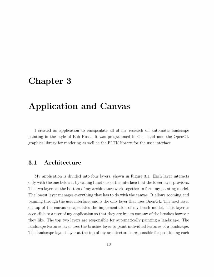
My application is divided into four layers, shown in Figure 3.1. Each layer interacts
only with the one below it by calling functions of the interface that the lower layer provides.
The two layers at the bottom of my architecture work together to form my painting model.
The lowest layer manages everything that has to do with the canvas. It allows zooming and
panning through the user interface, and is the only layer that uses OpenGL. The next layer
on top of the canvas encapsulates the implementation of my brush model. This layer is
accessible to a user of my application so that they are free to use any of the brushes however
they like. The top two layers are responsible for automatically painting a landscape. The
landscape features layer uses the brushes layer to paint individual features of a landscape.
The landscape layout layer at the top of my architecture is responsible for positioning each
13

14 Automated Landscape Painting in the Style of Bob Ross
Landscape Layout
Landscape Features
Brushes
Canvas
Set pixel colours
Paint brush strokes
Place landscape features
Paint Model
Automation
Figure 3.1: Layer architecture
of the landscape features on the canvas to create a final painting. Both of the landscape
layers are also accessible through the user interface of my application so that a user can
automatically paint individual landscape features one at a time or an entire landscape all
at once. The top three layers are each presented in further detail in the following chapters
while the canvas layer is presented in the next section.
3.2 Canvas
The most important service that the canvas layer provides is to set or get the colour of
any pixel on the surface of the canvas. The paint brushes layer needs to retrieve the colour
of a pixel on the canvas to facilitate paint blending, as discussed in detail in Chapter 4.

Chapter 3: Application and Canvas 15
3.2.1 Factors Influencing Design
There are three major factors that influence the design of the canvas layer, aside from
the requirements of setting and getting pixel colours anywhere on its surface.
The first design factor pertains to the viewing capabilities of the canvas. Most painting
applications support panning and zooming. I want my application to have this functionality
as well, mainly to make it easier to debug my painting code by being able to get a closer
look at the paint on the canvas.
Another factor under consideration for the design of the canvas layer is the size of the
canvas itself. The canvas Bob Ross used had a width of 24 inches and a height of 18 inches.
Not only do I have to accommodate this ratio, but I also have to choose an appropriate
number of pixels per inch. A number too small would prevent the canvas from displaying
enough detail, while a number too large could cause a significant decrease in performance.
The last factor influencing the design of the canvas is efficiency. Even though perfor-
mance is not a focus of my research, I still want users of my application to be able to
paint with the brushes at interactive speeds. Also, I want to render a complete landscape
painting in under 30 minutes on an average computer, thus beating the time it took Bob
Ross to paint an actual painting on his show. Since the canvas layer is at the lowest level
of my architecture, its services get used the most. Slow performance in this layer would
cripple my entire application.
3.2.2 Design
To accommodate the zoom and pan functionality that I want for the canvas, I decided at
the beginning to make the canvas a single, 2D rectangular polygon in 3D space. This allows
me to scale the polygon to create a zooming effect. It also allows me to implement panning
by simply translating the polygon within its plane. The canvas is viewed through an
OpenGL window. The alternative to choosing a rectangular polygon in space to represent
the canvas would be to draw the canvas directly to the pixels of a graphics window. One

16 Automated Landscape Painting in the Style of Bob Ross
way of doing this is to write pixels to the framebuffer of an OpenGL window using the
glDrawPixels function. The problem with this approach is that zooming and panning
become a more cumbersome task and would be slower than the first approach for canvases
of reasonable size.
I decided that I wanted the dimensions of the canvas to be roughly 1000× 750 pixels.
This is a reasonable size for a rendered painting with 40 pixels per inch. To obtain the
exact size in pixels, it was necessary to look into exactly how the paint would be updated
and displayed on the canvas. To display paint on the canvas, I use OpenGL textures.
However, OpenGL has a restriction on the size of textures you can use — the width and
height, excluding borders, must be a power of two. To accommodate the aspect ratio of
the canvas that Bob Ross used, the canvas in my application must have a size such that
the height is 75% of its width. No power of two is 75% of another power of two, so I cannot
cover the whole canvas polygon with only one texture. One solution to this problem is to
split the single canvas polygon into a grid of smaller polygons. I chose to split it into a
grid of 16 × 12 squares — 192 in total. Mapping a texture of size 64 × 64 pixels on each
square polygon causes the final canvas to be 1024 × 768 pixels in size. Since the canvas
has dimensions of 24× 18 inches, it has approximately 43 pixels per inch.
Splitting the canvas into smaller polygons not only allowed me to conform to OpenGL’s
texture constraints, but it also allows for efficient redrawing of the canvas. This comes from
the ability to selectively update the textures of only the polygonal tiles of the canvas that
get painted on, rather than all of the textures on the entire canvas. Whenever a pixel’s
colour on the canvas is changed, the square canvas piece that the altered pixel resides in is
marked as dirty. Whenever a redraw of the canvas is needed, only the textures of the dirty
canvas pieces are updated. See Figure 3.2 for an example of how this works. The tiles of
the canvas in the figure are smaller than normal size so that they can be differentiated.
A brush stroke is painted on the canvas and each tile that is affected by the stroke is
highlighted in red. Only the textures on the highlighted canvas polygons were updated
while the brush stroke was painted.
I made the choice of how many polygons to use and what size each texture should be

Chapter 3: Application and Canvas 17
Figure 3.2: Tiles of the canvas affected by a brush stroke
based on the size of a typical brush stroke on the canvas. The overhead of having too many
canvas tiles has to be balanced with updating the smallest possible area of the canvas. Too
many tiles causes too much overhead, while too few tiles causes unnecessary updates on
unused portions of the canvas. The size of the tiles is chosen so that there are as few as
possible, while being able to selectively update the smallest area of the canvas for typical
sized strokes. Obviously brush strokes can range in size quite a bit, so I estimated what
sizes would balance the overhead and typical update area the best for Bob Ross’s painting
style through experimentation.
3.3 Undo and Redo
The ability to undo and redo is important to the users of many interactive applications.
During development, it can also aid in rapid exploration of painting features by avoiding
restarts.
18 Automated Landscape Painting in the Style of Bob Ross
3.3.1 Simple Method
The easiest way to perform undo and redo operations in a painting application such as
mine is to push the state of the entire canvas onto a stack every time a reversible operation
is performed. This method works fine; however, it requires huge amounts of memory to
store the state of the entire canvas after every reversible operation. For example, my canvas
has dimensions of 1024 x 768 pixels, thus having 786,432 pixels in total. If three colours,
red, green, and blue, are each stored as one byte for each pixel, each state of the canvas
would require approximately 2.4 MB of memory to store on the stack. At a minimum, in
a painting application, you would want to have about 100 undo operations available, and
require 240 MB of memory. Also, each undo or redo would involve updating all of the
pixels of the entire canvas. Depending on how the canvas is implemented, each operation
may take an unacceptable amount of time to complete.
3.3.2 Improved Method
A better solution, which I implemented for my application, is to only store on the stack
the tiles of the canvas that get painted on, not the entire canvas. Since typical strokes
cover a small fraction of the total number of canvas tiles, this method saves great amounts
of memory and allows for many more undo and redo operations. Also, the act of restoring
a previous state of the canvas is much faster when only a fraction of it has to be retrieved
from the stack and redrawn. There is extra overhead in keeping track of which tiles were
painted on after each reversible operation; however, it is insignificant compared to the
savings in memory that this method provides.
3.4 User Interface
The user interface (UI) of my application was created using FLTK [4] so that it would
run on Windows, Linux, and MacOS. It has one OpenGL window that uses most of the

Chapter 3: Application and Canvas 19
real estate of the application to provide a view of the canvas. Other control windows used
to select options pertaining to the brushes or landscape features can be shown or hidden
through the main menu. The main menu at the top of the application window has the
typical options for file I/O and undo and redo you would expect in any application. It
also has menu options to resume, pause, or stop automatic painting as well as options to
choose which type of brush or landscape feature is currently active.
3.4.1 Painting Modes
My application has three mutually exclusive modes that a user can be in at any given
time. Fully manual mode is entered when a user selects a paint brush to use. Users can
use any of the brushes directly, similar to a normal painting program. Semi-automatic
mode is entered when the user selects a landscape feature to paint. They can choose
the attributes and select the painting location of any one landscape feature at a time.
Automatic mode is entered when the user selects a landscape layout. The entire landscape
is painted automatically in this mode and the user can just sit back and watch.
3.4.2 Options and Controls
The UI of my application provides access to all four layers of my architecture. A user
has control over the view of the canvas, the paint brushes, the landscape features, and the
landscape layout. The view of the canvas can be zoomed in and out using the scroll wheel
of the mouse. The right mouse button can be used to pan around the canvas. When all
of the layers work together, a user can render a landscape painting with one click of the
left mouse button on any part of the canvas. They can also select options for individual
landscape features and place them wherever they want on the canvas by clicking the left
mouse button. Furthermore, my application allows users to paint directly with all of the
brushes that I implemented, allowing them to paint whatever they want, whether it is a
landscape, a cityscape, or their favourite animal. All of the options pertaining to the paint

20 Automated Landscape Painting in the Style of Bob Ross
brushes including paint colour, pressure, and brush rotation are all available to the user.
Paint brush strokes are achieved by clicking the left mouse button and dragging through
the desired path of the stroke. Paint stabs can be achieved with any of the brushes simply
by pressing and releasing the left mouse button at the same location on the canvas.
3.4.3 Learning How To Paint Like Bob Ross
The results of the automatic painting that my application performs are not presented
to the user merely by displaying the final painting once it has completed. The techniques
used to paint each landscape feature are clearly visible because my application displays
and animates the progression of every single brush stroke. It is definitely not clear how a
painting is created when only examining the final image. However, watching the progression
of brush strokes used to create a painting, just as Bob Ross’s audience does, allows great
insight into how a painting can be reproduced. My application also displays the brush
parameters and options used for each automatically painted stroke in the same window
where a user would normally choose the parameters themselves when in fully manual
mode. This allows users to see things like which brush and paint colour is being used
by the currently painting stroke, as well as parameters like the current orientation of the
brush and how much pressure the current stroke is being applied with. I think having an
application show a user how to use itself is a good idea, especially for painting applications.
Novice users may not know of useful techniques or brush strokes that can easily create
surprisingly great results.

Chapter 4
Brushes
This chapter describes the larger component of my painting model that works together
with the canvas to produce working paint brushes. The brush layer is above the canvas
layer in my application’s software architecture and it encapsulates the implementation of
all of Bob Ross’s brushes. Although the focus of my research is not to create a brush
model, but rather to use one to paint a landscape, the brushes that I created are an
integral component of my work. Creating realistic paint brushes that are implemented
using real-world physics can be a complicated endeavour, as can be seen from Baxter’s
PhD thesis [10]. His work incorporates advanced physics and mathematics to model the
flow and viscosity of paint, the behaviour and geometry of brushes, and how they interact
with the canvas and each other. Instead, my goal in creating the brushes is to create the
simplest model that meets the requirements of my research.
It is a common practice in computer graphics to approximate the appearance of physical
phenomena with models that are far simpler than those characterized by the mathemat-
ical equations of real-world physics. A good example of this type of approximation is
Phong shading, which approximates how lighting affects the visual appearance of geomet-
ric objects. Obviously, the main benefit of approximating physical phenomena is a simpler
solution to the problem at hand. A simpler solution can also facilitate the benefit of higher
21

22 Automated Landscape Painting in the Style of Bob Ross
performance, which is desirable in my application.
Two factors become important in the design of my brush model because it is not a
physical simulation. The first is that there had to be a lot of trial and error and fine-tuning
of parameters to find which values best approximated real paint brushes. The process of
finding the right values for parameters such as the rate of paint loss and the amount of
blending from applied pressure became long and tedious at times. The other factor is
randomness. The way paint gets deposited from a brush onto a canvas seems to be quite
random. In other words, you never know exactly how a brush stroke will look until you have
actually done it. If every physical factor of a brush and paint is modelled correctly using
mathematics, the same randomness effect would be evident. This randomness is important
in creating a brush model that looks realistic and natural. To simulate this apparent
randomness using my simple brush model, several values of many of the brush parameters
are randomized within a specific threshold. Because of the randomness embedded in the
paint brushes, no two strokes ever look exactly the same.
Note that some aspects of my painting model are described in pixels while others in
inches. I alternate between them for clarity and convenience, but they can be converted
from one to another using the fact that there are 42.6 pixels per inch on the canvas.
4.1 Requirements
4.1.1 Different Kinds of Brushes
The main requirement of my brush model is that it has to accommodate the different
kinds of brushes that Bob Ross used to paint his landscape paintings. He used five different
kinds of brushes and a palette knife. He also used some brushes in different sizes. To
accommodate some of Bob Ross’s techniques, my brush model has to allow different ways
of using the same brush as well. For example, sometimes Bob Ross used only the corner
of the fan brush instead of the entire width.

Chapter 4: Brushes 23
4.1.2 General Operations
There are several operations that can be performed with any kind of brush. These
include
• painting a stroke in a straight line from one point on the canvas to another
• stabbing with a brush at one point on the canvas
• loading and reloading a brush with paint of a specific colour and amount
• rotating a brush around its handle axis
• changing the applied pressure of a brush on the canvas
The brush layer offers the two most basic types of strokes — a line stroke and a stab stroke.
A line stroke follows a straight line path from one point on the canvas to another. A stab
of the brush is only at one point on the canvas. Other, more complicated, strokes can be
constructed from a sequence of line strokes. Brush rotation and pressure are specified at
the endpoints of a line stroke, and linearly interpolated along its length.
4.1.3 Blending
In a basic brush model, like the one found in Microsoft R© Paint, paint that is applied
to the canvas using a brush simply overlaps any of the existing paint and does not interact
with it at all. This type of model cannot be used to simulate Bob Ross’s brushes. Bob
Ross used a wet-on-wet painting technique [14]. This means that he never painted on a dry
surface. Even before he began to paint, he would always cover the entire canvas in a thin
layer of liquid white paint. This technique of always working with wet paint on the canvas
allowed him to achieve a variety of beautiful blending effects depending on what kind of
brush strokes he used. The fact that my brushes have to model this type of paint blending
means two things. The first is that since all brush strokes are carried out over wet paint, a

24 Automated Landscape Painting in the Style of Bob Ross
brush must appear to pick up paint off the canvas. Secondly, since two different colours of
wet paint can interact, my brush model must also give the illusion that paints of different
colours can be mixed together to form new colours. For example, if a brush is loaded with
yellow paint and then used to paint over an area of the canvas that has red paint on it,
the paint that remains on the brush throughout the stroke should gradually turn orange.
Having to implement paint blending greatly increases the minimum amount of complex-
ity that my brush model can have. My original goal of creating the simplest brush model
that meets the requirements of my research still holds, however. There are many complex
ways of implementing paint blending, but I use a straightforward way that achieves the
blending effects that I need to capture the results of Bob Ross’s wet-on-wet technique.
4.2 Painting Entities
The main idea for my brush model is to create brushes by combining a set of self-
sufficient entities to form the shape of each individual brush. An individual entity can be
easily thought of as a single bristle, or a clump of bristles that behave uniformly because
they are stuck together by paint. I do not want to restrict the conceptual model of these
entities to be bristles of a brush, however, since they are also used to model the palette
knife. I will refer to each of them as a painting entity (PE) hereafter.
4.2.1 Paint Amount and Colour
Each PE can have a certain amount of paint of a certain colour at any given time. The
amount of paint that is currently on a PE is described as a real number between 0 and 100.
The colour of the paint is described as an RGB triple where each component is a number
between 0 and 255, inclusively. As a PE deposits paint onto the canvas, the amount of
paint it has on it decreases and the colour of the paint can change according to the rules
of blending described later on.

Chapter 4: Brushes 25
Figure 4.1: Drops of paint
4.2.2 A Drop of Paint
The paint that is deposited by a PE at a single location of the canvas is depicted by
nine pixels arranged in a square and centred at that canvas location. Each of these deposits
of paint will be referred to as a drop of paint hereafter. See Figure 4.1 for a zoomed in
view of four drops of a blue coloured paint. The fundamental action of painting occurs
when a PE is either dragged through a straight line on the canvas to form a stroke or is
stabbed on the canvas at one location. If a PE is stabbed on the canvas, a square of nine
pixels of paint is deposited on the canvas at the stab location. If the PE is stroked through
a line, a square of nine pixels of paint is deposited on the canvas at each pixel between the
endpoints of the line. PEs are thus directly interacting with the canvas layer, as their job
is to change the colour of appropriate pixels on the canvas to make it appear as if it has
been painted on. The colour of each pixel changed by a PE is decided by three things: the
colour of the paint currently on the PE, the original colour of the pixel on the canvas at
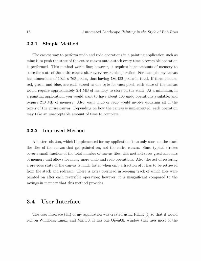
the same location, and the alpha value assigned to the pixel. See Figure 4.2 for a zoomed
in view of a stroke painted with one PE. The stroke is comprised of a set of paint drops
painted through line segments defined by successive samples of the mouse cursor location.
This stroke was created from five line segments and contains 21 drops of paint.
26 Automated Landscape Painting in the Style of Bob Ross
Figure 4.2: A stroke created with one painting entity
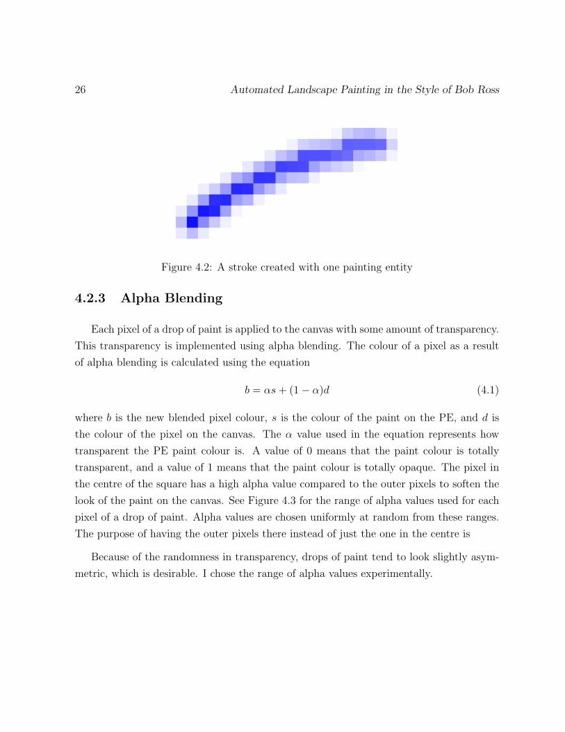
4.2.3 Alpha Blending
Each pixel of a drop of paint is applied to the canvas with some amount of transparency.
This transparency is implemented using alpha blending. The colour of a pixel as a result
of alpha blending is calculated using the equation
b = αs + (1− α)d (4.1)
where b is the new blended pixel colour, s is the colour of the paint on the PE, and d is
the colour of the pixel on the canvas. The α value used in the equation represents how
transparent the PE paint colour is. A value of 0 means that the paint colour is totally
transparent, and a value of 1 means that the paint colour is totally opaque. The pixel in
the centre of the square has a high alpha value compared to the outer pixels to soften the
look of the paint on the canvas. See Figure 4.3 for the range of alpha values used for each
pixel of a drop of paint. Alpha values are chosen uniformly at random from these ranges.
The purpose of having the outer pixels there instead of just the one in the centre is
Because of the randomness in transparency, drops of paint tend to look slightly asym-
metric, which is desirable. I chose the range of alpha values experimentally.
Chapter 4: Brushes 27
[0.01, 0.03]
[0.01, 0.03][0.01, 0.03]
[0.4, 0.6] [0.05, 0.07]
[0.05, 0.07]
[0.05, 0.07]
[0.05, 0.07]
[0.01, 0.03]
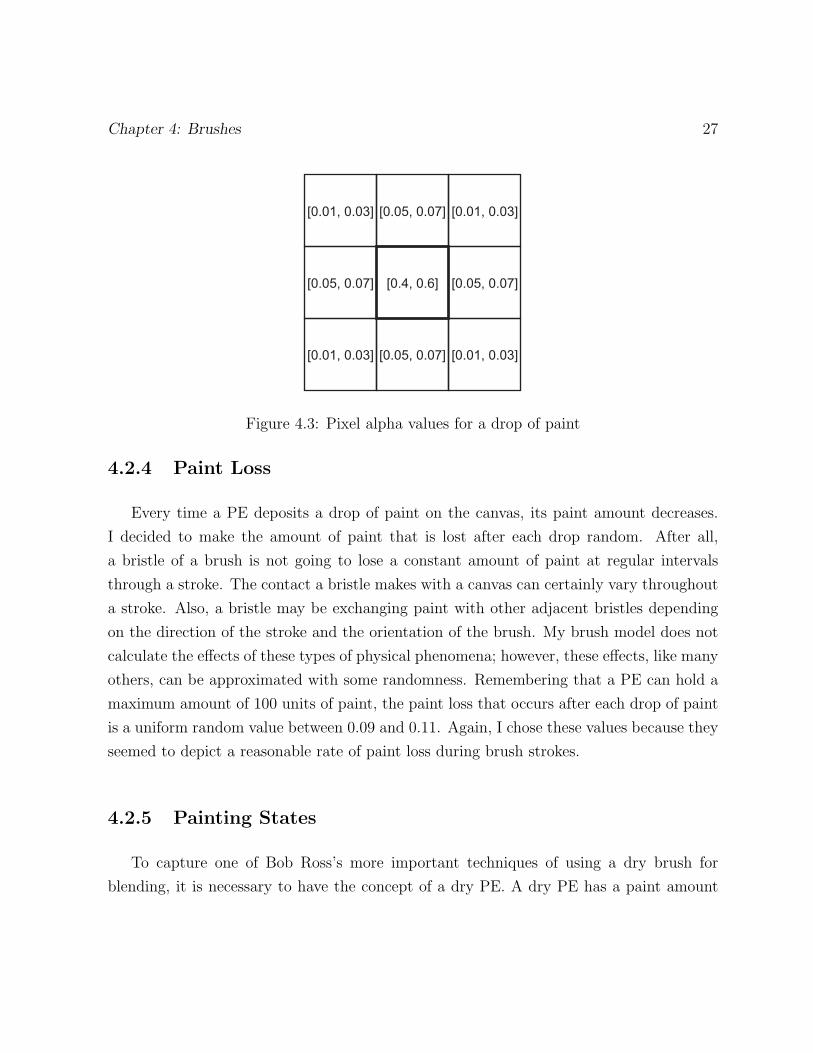
Figure 4.3: Pixel alpha values for a drop of paint
4.2.4 Paint Loss
Every time a PE deposits a drop of paint on the canvas, its paint amount decreases.
I decided to make the amount of paint that is lost after each drop random. After all,
a bristle of a brush is not going to lose a constant amount of paint at regular intervals
through a stroke. The contact a bristle makes with a canvas can certainly vary throughout
a stroke. Also, a bristle may be exchanging paint with other adjacent bristles depending
on the direction of the stroke and the orientation of the brush. My brush model does not
calculate the effects of these types of physical phenomena; however, these effects, like many
others, can be approximated with some randomness. Remembering that a PE can hold a
maximum amount of 100 units of paint, the paint loss that occurs after each drop of paint
is a uniform random value between 0.09 and 0.11. Again, I chose these values because they
seemed to depict a reasonable rate of paint loss during brush strokes.
4.2.5 Painting States
To capture one of Bob Ross’s more important techniques of using a dry brush for
blending, it is necessary to have the concept of a dry PE. A dry PE has a paint amount
28 Automated Landscape Painting in the Style of Bob Ross
of zero, but its blending capabilities can be used to move existing paint on the canvas to
different locations. To accommodate the fact that a PE can run dry, I had to establish
four different states that a PE can be in at any given time. I implement paint blending
differently depending on which state a PE is in. The four states are
• Wet With Loaded Paint: A PE is in this state if it has an amount of loaded paint
on it that is greater than zero.
• Drying From Loaded Paint: A PE is in this state when its loaded paint has just
been depleted to zero.
• Dry With Canvas Paint: A PE is in this state if it does not have any loaded paint
on it, but does have paint that was picked up from the canvas.
• Dry With No Paint: A PE is in this state if it does not have any paint on it at
all. It has not touched the canvas since it was cleaned.
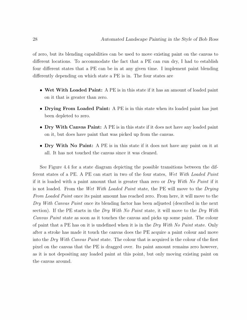
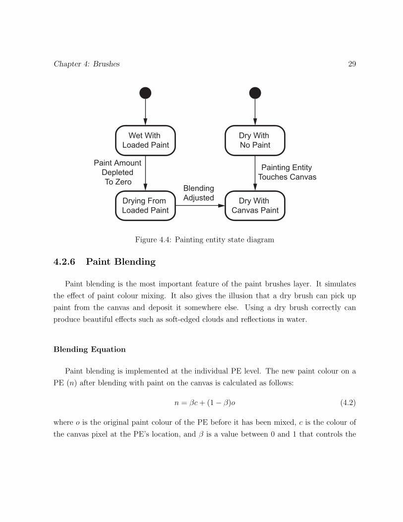
See Figure 4.4 for a state diagram depicting the possible transitions between the dif-
ferent states of a PE. A PE can start in two of the four states, Wet With Loaded Paint
if it is loaded with a paint amount that is greater than zero or Dry With No Paint if it
is not loaded. From the Wet With Loaded Paint state, the PE will move to the Drying
From Loaded Paint once its paint amount has reached zero. From here, it will move to the
Dry With Canvas Paint once its blending factor has been adjusted (described in the next
section). If the PE starts in the Dry With No Paint state, it will move to the Dry With
Canvas Paint state as soon as it touches the canvas and picks up some paint. The colour
of paint that a PE has on it is undefined when it is in the Dry With No Paint state. Only
after a stroke has made it touch the canvas does the PE acquire a paint colour and move
into the Dry With Canvas Paint state. The colour that is acquired is the colour of the first
pixel on the canvas that the PE is dragged over. Its paint amount remains zero however,
as it is not depositing any loaded paint at this point, but only moving existing paint on
the canvas around.
Chapter 4: Brushes 29
Wet With Loaded Paint
Dry With No Paint
Drying From Loaded Paint
Dry With Canvas Paint
Paint Amount Depleted To Zero
Painting Entity Touches Canvas
BlendingAdjusted
Figure 4.4: Painting entity state diagram
4.2.6 Paint Blending
Paint blending is the most important feature of the paint brushes layer. It simulates
the effect of paint colour mixing. It also gives the illusion that a dry brush can pick up
paint from the canvas and deposit it somewhere else. Using a dry brush correctly can
produce beautiful effects such as soft-edged clouds and reflections in water.
Blending Equation
Paint blending is implemented at the individual PE level. The new paint colour on a
PE (n) after blending with paint on the canvas is calculated as follows:
n = βc + (1− β)o (4.2)
where o is the original paint colour of the PE before it has been mixed, c is the colour of
the canvas pixel at the PE’s location, and β is a value between 0 and 1 that controls the

30 Automated Landscape Painting in the Style of Bob Ross
0.001
Increasing Paint Amount
Increasing Pressure
Wet Blending Dry Blending
1
0.03 0.2 0.95
0
Figure 4.5: Blending amount chart
amount of paint blending that occurs between the paint on the PE and the paint on the
canvas.
You can see from Equation 4.2 that if β = 0, there is no paint mixing at all. The new
paint colour of the PE would equal the old paint colour and the paint on the canvas would
have no effect. Conversely, if β = 1, the PE immediately takes the canvas colour. Choosing
values for the blend amount between 0 and 1 and applying this calculation sequentially for
a number of drops of paint in a row produces the effect of the original paint colour on a
PE gradually blending toward the colour of paint on the canvas.
Blending Amount Values
By visually examining the effects of different values for the blending amount, I was
able to establish which values looked the most convincing for both wet and dry PEs. See
Figure 4.5 for a chart of the ranges of blending amount values. To establish the best values
for the blending amounts of wet and dry PEs, I examined how they looked when they were
used in a brush. This is because it is hard to gauge how much blending the paint on a
single PE should be doing.
When a PE is wet and loaded with a paint amount greater than zero, the blending
amount used is between 0.001 and 0.03. The value that is used within this range is
determined by the paint amount. This is because if there is a lot of paint on a brush, the
paint will blend to the paint colours on the canvas more slowly than if there is little paint
on the brush. I use 0.001 as the blending amount for a paint amount of 100, 0.03 for a
Chapter 4: Brushes 31
paint amount of 1, and linearly interpolate in between.
For a dry brush, things get a little trickier. I found that a high blending amount near 1
makes a dry brush seem like it is passing over the canvas lightly, while a blending amount
of around 0.2 makes it seem like a dry brush is being pushed down on the canvas quite
hard. This is because with a high blending amount, a paint colour picked up off the canvas
blends quickly to any surrounding paint colour so it appears as if only a small amount of
paint is being moved across the canvas. Conversely, with a blending amount around 0.2, it
takes longer for a paint colour picked up off the canvas to blend to any surrounding paint
colour so it appears as if more paint is being moved across the canvas. So, I decided to
use the applied pressure parameter of a brush to vary the blending amount used for each
of the brush’s PEs. I use 0.2 as the blending amount for a pressure of 100 and 0.95 for a
pressure of 1. I linearly interpolate between 0.2 and 0.95 for paint amounts between 100
and 1.
Now there is the question of what happens when a PE goes from being wet to dry.
Having a PE instantaneously jump from a blending amount in the wet range to a blending
amount in the dry range does not look realistic. This is what the Drying From Loaded
Paint state is for, previously shown in Figure 4.4. During this state, the blending amount
used for a PE changes gradually from its wet blending amount to its dry blending amount.
Specifically, the PE’s blending amount increases by 0.01 after each drop of paint until it
reaches its dry blending amount. When it reaches its dry blending amount, the PE’s state
changes to Dry With Canvas Paint, as can be seen from the Blending Adjusted transition
in Figure 4.4.
Finally, a more organic look for a brush is achieved by randomly adjusting the blending
amount of each PE by a uniformly chosen percentage between −3 and 3.
Results
Figure 4.6 shows an example of a dry 1 inch brush in action. Two strokes were painted
horizontally in red and blue paint. Then, five vertical strokes with a dry brush were painted
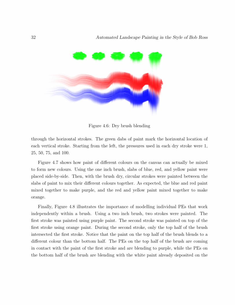
32 Automated Landscape Painting in the Style of Bob Ross
Figure 4.6: Dry brush blending
through the horizontal strokes. The green dabs of paint mark the horizontal location of
each vertical stroke. Starting from the left, the pressures used in each dry stroke were 1,
25, 50, 75, and 100.
Figure 4.7 shows how paint of different colours on the canvas can actually be mixed
to form new colours. Using the one inch brush, slabs of blue, red, and yellow paint were
placed side-by-side. Then, with the brush dry, circular strokes were painted between the
slabs of paint to mix their different colours together. As expected, the blue and red paint
mixed together to make purple, and the red and yellow paint mixed together to make
orange.
Finally, Figure 4.8 illustrates the importance of modelling individual PEs that work
independently within a brush. Using a two inch brush, two strokes were painted. The
first stroke was painted using purple paint. The second stroke was painted on top of the
first stroke using orange paint. During the second stroke, only the top half of the brush
intersected the first stroke. Notice that the paint on the top half of the brush blends to a
different colour than the bottom half. The PEs on the top half of the brush are coming
in contact with the paint of the first stroke and are blending to purple, while the PEs on
the bottom half of the brush are blending with the white paint already deposited on the

Chapter 4: Brushes 33
Figure 4.7: Paint mixing
Figure 4.8: Individual painting entity blending within a brush
canvas to form a light orange colour. The resulting paint colours on the brush after the
second stroke can be seen before the brush goes dry when the stroke pulls away from the
original at the end. Using independent PEs to construct a brush in my painting model
makes it easy to achieve the necessary effect of being able to have more than one colour of
paint on a brush at the same time.
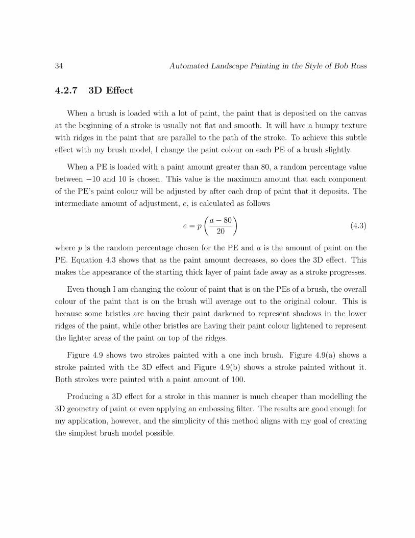
34 Automated Landscape Painting in the Style of Bob Ross
4.2.7 3D Effect
When a brush is loaded with a lot of paint, the paint that is deposited on the canvas
at the beginning of a stroke is usually not flat and smooth. It will have a bumpy texture
with ridges in the paint that are parallel to the path of the stroke. To achieve this subtle
effect with my brush model, I change the paint colour on each PE of a brush slightly.
When a PE is loaded with a paint amount greater than 80, a random percentage value
between −10 and 10 is chosen. This value is the maximum amount that each component
of the PE’s paint colour will be adjusted by after each drop of paint that it deposits. The
intermediate amount of adjustment, e, is calculated as follows
e = p
(a− 80
20
)(4.3)
where p is the random percentage chosen for the PE and a is the amount of paint on the
PE. Equation 4.3 shows that as the paint amount decreases, so does the 3D effect. This
makes the appearance of the starting thick layer of paint fade away as a stroke progresses.
Even though I am changing the colour of paint that is on the PEs of a brush, the overall
colour of the paint that is on the brush will average out to the original colour. This is
because some bristles are having their paint darkened to represent shadows in the lower
ridges of the paint, while other bristles are having their paint colour lightened to represent
the lighter areas of the paint on top of the ridges.
Figure 4.9 shows two strokes painted with a one inch brush. Figure 4.9(a) shows a
stroke painted with the 3D effect and Figure 4.9(b) shows a stroke painted without it.
Both strokes were painted with a paint amount of 100.
Producing a 3D effect for a stroke in this manner is much cheaper than modelling the
3D geometry of paint or even applying an embossing filter. The results are good enough for
my application, however, and the simplicity of this method aligns with my goal of creating
the simplest brush model possible.

Chapter 4: Brushes 35
(a) With 3D effect (b) Without 3D effect
Figure 4.9: Comparison of strokes with and without the 3D effect
4.3 General Brush Operations and Attributes
Now that I have described a painting model for individual PEs, I discuss how brushes
are created from a set of PEs. This section describes the common operations and attributes
across all of the different kinds of brushes. Some brushes, like the palette knife, have special
functionality that is not shared with other kinds of brushes. The subsequent sections
describe the unique operations and attributes of each brush.
An important simplifying aspect of my brush model is that most of the functionality
performed by a brush can be delegated to its individual PEs. Since each PE is capable
of painting on its own, the role of a brush in my paint brushes layer is ultimately not to
paint, but to manage its PEs.
4.3.1 Painting Entity Locations
I create a brush by placing a number of PEs together to form a shape that resembles
the footprint of the brush. When it is time to reset the PEs of a brush, each PE is assigned
a location relative to the centre point of the brush footprint. The PE locations of a brush
are randomly chosen each time a stroke is about to begin, adding to the randomness of
each stroke. Brushes of different kinds and size require different ways of choosing their

36 Automated Landscape Painting in the Style of Bob Ross
Figure 4.10: Brush rotations
PE locations. The algorithms used to choose the PE locations for each type of brush are
described at the end of this chapter.
4.3.2 Brush Orientation
Every brush can be rotated through a complete circle by rotating every PE around
the centre point of the brush. See Figure 4.10 for a picture of eight stabs of paint using
different orientations of the fan brush. Starting from the top and proceeding clockwise,
the rotations that were used in degrees are 0, 45, 90, 135, 180, 225, 270, and 315.
4.3.3 Paint Loading
To load a brush with a certain amount and colour of paint, I simply have to load the
paint on each PE of the brush. It can be expected that not all of the bristles on a brush
will be loaded with exactly the same amount of paint. I load a random paint amount on
each PE; the amount specified is adjusted by a random percentage between −5 and 5.
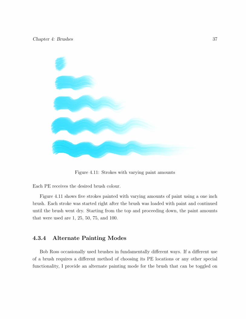
Chapter 4: Brushes 37
Figure 4.11: Strokes with varying paint amounts
Each PE receives the desired brush colour.
Figure 4.11 shows five strokes painted with varying amounts of paint using a one inch
brush. Each stroke was started right after the brush was loaded with paint and continued
until the brush went dry. Starting from the top and proceeding down, the paint amounts
that were used are 1, 25, 50, 75, and 100.
4.3.4 Alternate Painting Modes
Bob Ross occasionally used brushes in fundamentally different ways. If a different use
of a brush requires a different method of choosing its PE locations or any other special
functionality, I provide an alternate painting mode for the brush that can be toggled on

38 Automated Landscape Painting in the Style of Bob Ross
and off. Examples of this include using only the corner of a fan brush instead of the entire
width or using the corner of a palette knife to scratch in fine lines in any paint already on
the canvas. Rather than model the brush geometry in a sophisticated way that accounts
for these uses, different PE locations and functionality are employed to implement these
uses instead.
4.3.5 Strokes
The brush layer offers two different types of strokes with any kind of brush. A line
stroke is painted along a straight line path between two points. A stab stroke models the
brush being pushed against the canvas at only one location.
Line Stroke
A line stroke is specified by a start and end location on the canvas and can have
different start and end parameters for brush rotation and pressure. Intermediate values
for the rotation and pressure are linearly interpolated through the stroke. The first step
to paint a line stroke is to find points on the line between the start and end locations,
sampled at regular intervals. The locations of PEs are found at each sample point using
their offset from the centre point of the brush and the interpolated brush rotation. Then,
a straight line of paint drops is deposited on the canvas by each PE between each of their
calculated locations from the sample points on the line.
Stab
A stab stroke is specified by a single canvas location, brush rotation, and pressure.
There are also two other parameters used to define a stab stroke: offset and direction.
The stab offset describes how much the bristles of a brush slide across the canvas during
a stab. The stab offset can be thought of as being correlated to the angle that a brush
Chapter 4: Brushes 39
makes with the canvas during a stab. An angle of close to 90 degrees from the canvas
will cause the least amount of offset of the bristles during a stab, while an angle close
to 0 degrees from the canvas will cause the most. There are also other factors that may
influence the stab offset like applying varied pressure or twisting the brush during the stab
to make the bristles bend and slide on the canvas. Instead of relating the amount of stab
offset to a realistic property of a brush, I simply allow the interface for stabbing to accept
an amount between 0 and 5, inclusively. The stab offset amount represents how many
consecutive drops of paint will be deposited in a line by each PE of a brush during the
stab. The line starts at the original location of a PE. Where it ends depends on the stab’s
direction.
The direction of the line of paint drops deposited by each PE during a stab is specified
by the stab direction. The angle of stab direction is distinct from a brush’s orientation
angle. Each stab of a brush is actually a small stroke where the starting point is the location
of the stab and the endpoint is calculated from the stab offset and direction. When the
stab offset is small (0–2), the stab direction does not have much affect on appearance. See
Figure 4.12 for examples of stabs using different parameters with a two inch brush. The
stab offsets used for each column start at 0 on the left and end at 5 on the right. The stab
directions used for each row, starting from the top, are 0, 45, and 90 degrees.
4.4 One and Two Inch Brushes
I create the shape of the footprint of the one and two inch brushes using an ellipse. The
length of the major axes of the ellipses used for both sizes of brushes are the same as their
described size, 1 and 2 inches, respectively. I use 0.6 inches for the minor axis of the ellipse
for the two inch brush and 0.55 inches for the minor axis of the one inch brush. I chose
the values for the minor axes, or thickness of the brushes, based on a visual inspection of
how the brushes looked while being used in my program.
The ellipses chosen as the footprint shapes for the these brushes serve as bounding

40 Automated Landscape Painting in the Style of Bob Ross
Figure 4.12: Brush stabs using different parameters
regions for where the PEs of the brushes can be located. The centre point of a brush
is located at the centre of its bounding ellipse. The initial PE locations are chosen by
stratified sampling. I divide the ellipse’s bounding box into a grid of locations and place a
PE at each location. Locations in the grid are placed 2 pixels apart in the x direction and
1 pixel apart in the y direction. To make the PE locations more random than a predictable
grid layout bounded by an ellipse, each location is randomly offset by a maximum of ±1
pixel in both the x and y directions before it is checked to see if it is within the bounding
ellipse and thus included as a PE of the brush. See Figure 4.13 for a simplified diagram
illustrating how a fraction of the typical amount of PE locations would be chosen. Notice
that some of the locations that would have been included in the brush before randomization
are not within the bounding ellipse after randomization, and vice-versa. The result of this
is that the footprint of the brush ends up having a randomly shaped silhouette instead of
the edges of the brush looking like the outline curve of the bounding ellipse.
The number of PEs each brush has is actually random each time because of the ran-
domized PE locations. The two inch brush has around 300 PEs (the most of any kind of
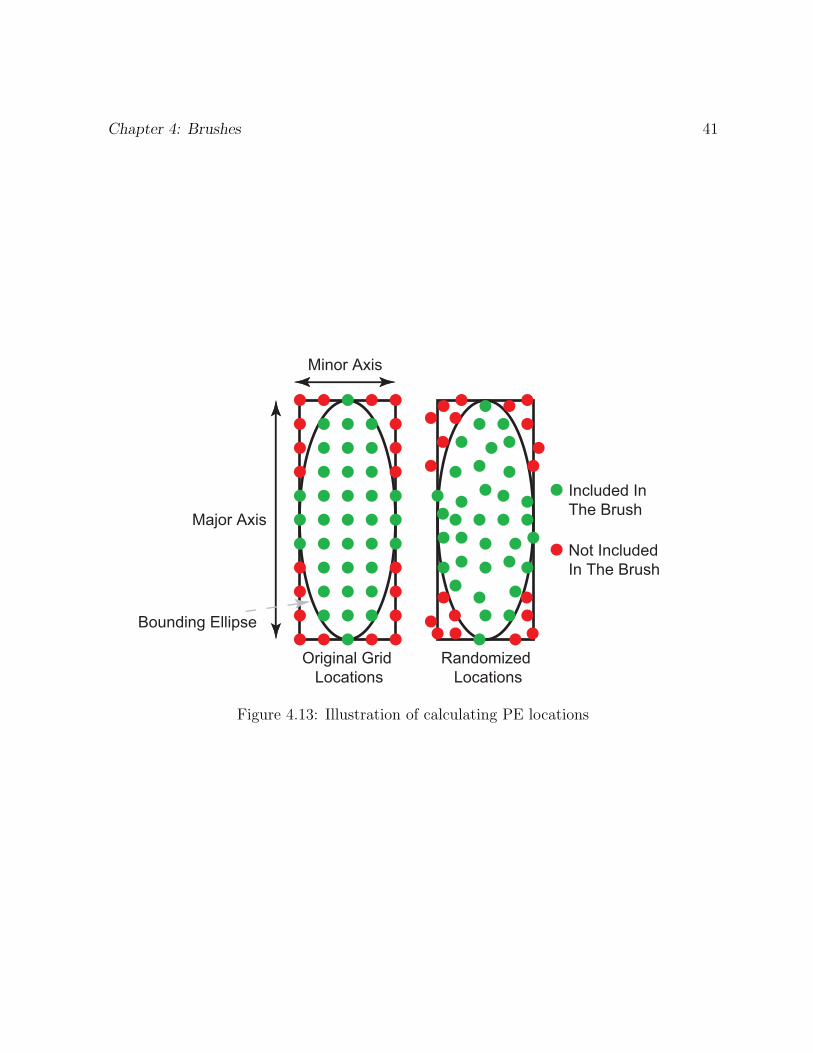
Chapter 4: Brushes 41
Included In The BrushMajor Axis
Minor Axis
Not Included In The Brush
Bounding Ellipse
Randomized Locations
Original Grid Locations
Figure 4.13: Illustration of calculating PE locations

42 Automated Landscape Painting in the Style of Bob Ross
Figure 4.14: Brush strokes using the one and two inch brushes
brush), while the one inch brush has around 135 PEs. See Figure 4.14 for examples of
brush strokes using the 1 and 2 inch brushes.
4.5 Round Brush
I created the round brush in the same way as the one and two inch brushes. In fact, the
only difference between them is the shape of the bounding ellipse. For the round brush,
the major axis has a length of 1 inch, while the minor axis has a length of 0.8 inches. These
dimensions give the round brush a more circular footprint than the one inch brush. See
Figure 4.15 for examples of brush strokes using the round brush.

Chapter 4: Brushes 43
Figure 4.15: Brush strokes using the round brush
4.6 Fan Brush
Bob Ross used the fan brush in several different ways. One of his techniques involved
painting stab strokes at different pressures in order to use a different amount of the bristles
of the brush. This allowed him to create stab strokes of different sizes using the same size
of brush. Also, sometimes he used only the corner of the fan brush to apply a stab stroke
of a different shape than if the entire brush had been used. I handle these two techniques
by changing the shape of the footprint of the fan brush in different ways.
The footprint of the fan brush is calculated using two ellipses. One of the ellipses,
called the container ellipse hereafter, has a section of its area allocated as the bounding
region for the PE locations. Another ellipse, called the boundary ellipse hereafter, is used
to adjust the size of the bounding region within the container ellipse by overlapping it and
creating a boundary with a segment of its outline. See Figure 4.16 for a diagram showing
the ellipses and the bounding region for the PE locations.
4.6.1 Symmetric Footprint
To obtain a symmetric footprint, the container and boundary ellipses are centred at
the same point. I will not use the terms minor and major axes to describe the size of the
ellipses because they are in opposite directions for each ellipse and it could get confusing.

44 Automated Landscape Painting in the Style of Bob Ross
Container Ellipse
Boundary Ellipse
PE LocationBounding Region
Figure 4.16: Fan brush footprint calculation
Instead, I will just use width and height. The width of the container ellipse is 0.6 inches
and its height is 1 inch. The width of the boundary ellipse is 0.4 inches. The height of the
boundary ellipse changes depending on what pressure is used. This is how I accommodate
for footprints of different sizes at different pressures. The greater the pressure, the smaller
the height of the boundary ellipse, and the larger the bounding region. The smaller the
pressure, the greater the height, and the smaller the bounding region. The height of the
container ellipse is linearly interpolated between 1.3 and 1.0 for pressures between 1 and
100.
See Figure 4.17 for a succession of stabs made with the fan brush using different pres-
sures. Starting from the left, the pressures used are 1, 20, 40, 60, 80, and 100. Although
the differences in the stabs are subtle, you can see that more of the round shape of the
brush emerges as the pressure increases. This is because more of the bristles of a brush
would be spreading out and touching a canvas at higher applied pressures.
See Figure 4.18 for an example of a few strokes made using the fan brush.

Chapter 4: Brushes 45
Figure 4.17: Stabs made using the fan brush symmetrically
Figure 4.18: Strokes made using the fan brush
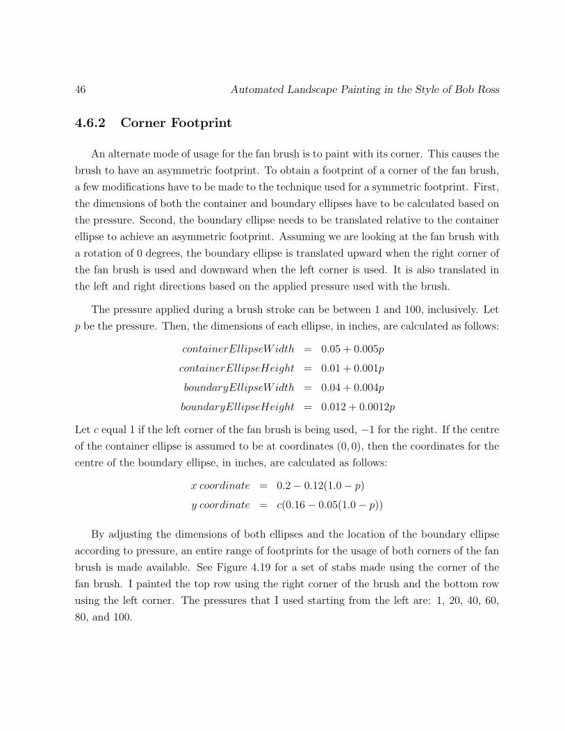
46 Automated Landscape Painting in the Style of Bob Ross
4.6.2 Corner Footprint
An alternate mode of usage for the fan brush is to paint with its corner. This causes the
brush to have an asymmetric footprint. To obtain a footprint of a corner of the fan brush,
a few modifications have to be made to the technique used for a symmetric footprint. First,
the dimensions of both the container and boundary ellipses have to be calculated based on
the pressure. Second, the boundary ellipse needs to be translated relative to the container
ellipse to achieve an asymmetric footprint. Assuming we are looking at the fan brush with
a rotation of 0 degrees, the boundary ellipse is translated upward when the right corner of
the fan brush is used and downward when the left corner is used. It is also translated in
the left and right directions based on the applied pressure used with the brush.
The pressure applied during a brush stroke can be between 1 and 100, inclusively. Let
p be the pressure. Then, the dimensions of each ellipse, in inches, are calculated as follows:
containerEllipseWidth = 0.05 + 0.005p
containerEllipseHeight = 0.01 + 0.001p
boundaryEllipseWidth = 0.04 + 0.004p
boundaryEllipseHeight = 0.012 + 0.0012p
Let c equal 1 if the left corner of the fan brush is being used, −1 for the right. If the centre
of the container ellipse is assumed to be at coordinates (0, 0), then the coordinates for the
centre of the boundary ellipse, in inches, are calculated as follows:
x coordinate = 0.2− 0.12(1.0− p)
y coordinate = c(0.16− 0.05(1.0− p))
By adjusting the dimensions of both ellipses and the location of the boundary ellipse
according to pressure, an entire range of footprints for the usage of both corners of the fan
brush is made available. See Figure 4.19 for a set of stabs made using the corner of the
fan brush. I painted the top row using the right corner of the brush and the bottom row
using the left corner. The pressures that I used starting from the left are: 1, 20, 40, 60,
80, and 100.

Chapter 4: Brushes 47
Figure 4.19: Stabs made using the corner of the fan brush
4.6.3 Painting Entity Placement
Once the bounding region of the footprint is established with the container and bound-
ary ellipses, the PE locations for the brush are chosen. Like the previous brushes, a grid
of locations is used to determine the PE locations. The grid spans the left half of the
bounding rectangle of the container ellipse. I found that I had to create a denser grid
of locations for the fan brush than I did for the one and two inch or round brushes to
accommodate its more intricate shape. The locations are placed at every pixel in the x
direction and at every other pixel in the y direction. After randomizing each location by a
maximum of ±1 pixel in both the x and y directions, each location is checked to see if it
is inside of the container ellipse and outside of the boundary ellipse. If it is, that location
becomes the location of a PE for the brush.
4.7 Filbert Brush
The filbert brush has a circular footprint that changes size with pressure and is smaller
than the other brushes I have discussed so far. Let p be the applied pressure. The bounding
region for the PE locations is a circle with a diameter d in inches, calculated by the following
equation:
d = 0.025 + 0.00225p (4.4)

48 Automated Landscape Painting in the Style of Bob Ross
Figure 4.20: Strokes made using the filbert brush
Equation 4.4 yields a maximum diameter of 0.25 inches at a pressure of 100.
The grid locations for potential PEs span the bounding square of the circular bounding
region. The locations are spaced tightly, occupying every pixel of the grid before random-
ization. The reason for this is that a filbert brush seems to have tightly packed bristles to
paint lines and curves that are highly defined and are mostly used to add detail.
Figure 4.20 shows a few strokes and stabs made using the filbert brush. The stroke at
the bottom illustrates the effect of varying the pressure to obtain a progressively smaller
brush footprint within a stroke. That stroke started with a pressure of 100 and ended at
1. As the pressure changes dynamically, the PE distribution of the brush does not change
— only fewer PEs are used.
4.8 Liner Brush
The liner brush is by far the smallest brush that Bob Ross used. Its purpose is to add
fine detail or touch-ups to a painting. One of the ways that Bob Ross used the liner brush
was to add his signature to a painting once he had completed it. Creating the liner brush
with my brush model is quite simple. Only one PE location is used at the centre point
of the brush, so no bounding region is necessary. As for the number of PEs that should
be placed at the centre location, I found that only one seems to approximate a real liner
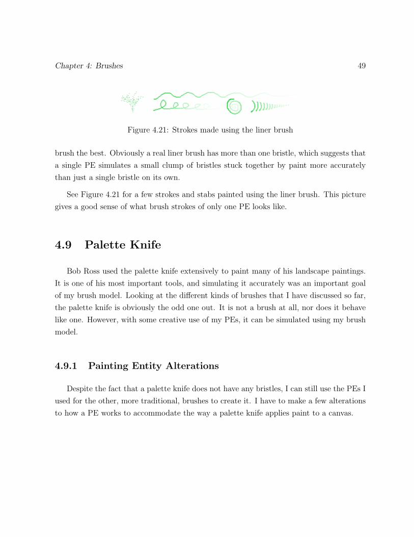
Chapter 4: Brushes 49
Figure 4.21: Strokes made using the liner brush
brush the best. Obviously a real liner brush has more than one bristle, which suggests that
a single PE simulates a small clump of bristles stuck together by paint more accurately
than just a single bristle on its own.
See Figure 4.21 for a few strokes and stabs painted using the liner brush. This picture
gives a good sense of what brush strokes of only one PE looks like.
4.9 Palette Knife
Bob Ross used the palette knife extensively to paint many of his landscape paintings.
It is one of his most important tools, and simulating it accurately was an important goal
of my brush model. Looking at the different kinds of brushes that I have discussed so far,
the palette knife is obviously the odd one out. It is not a brush at all, nor does it behave
like one. However, with some creative use of my PEs, it can be simulated using my brush
model.
4.9.1 Painting Entity Alterations
Despite the fact that a palette knife does not have any bristles, I can still use the PEs I
used for the other, more traditional, brushes to create it. I have to make a few alterations
to how a PE works to accommodate the way a palette knife applies paint to a canvas.

50 Automated Landscape Painting in the Style of Bob Ross
Disable Paint Blending
The first alteration required is to disable paint blending. The reason for this is that
the paint that is deposited onto a canvas from a palette knife is, in a way, rolled on top of
whatever paint that may already exist on the canvas. A knife’s edge does not mix paint
together nearly as well as the hundreds of slender bristles found on a brush. Although
paints of different colours can be mixed together on a palette using a knife, over the course
of a typical painting stroke, any paint blending is imperceptible. Bob Ross’s use of the
palette knife is consistent with this observation.
The paint blending of a PE used for a palette knife is only disabled when it has a paint
amount greater than 0. When a palette knife is used dry, paint blending is enabled for all
of its PEs so that the effect of using a dry knife to move small amounts of paint on the
canvas is still available.
Disable 3D Effect
The 3D effect applied to the paint deposited on the canvas using a brush with a paint
amount of more than 80 is disabled for the palette knife. Lightening and darkening the
paint colour on various PEs used for the knife does not produce the correct 3D effect
required for a thick layer of paint coming off of a knife. The paint coming off of a knife
is generally flat with slight, shallow undulations that span a lot more area than the ridges
produced from a brush. A more complex approach would need to be implemented to
produce this effect for the palette knife and since the 3D effect is not even required and is
just a simple improvement I added to the brushes, I did not implement it for the palette
knife.

Chapter 4: Brushes 51
Allow Painting to be Disabled
Another change to the PE model is to add a flag that can be set for each PE that
disables it from painting. While a PE has been disabled from depositing paint on the
canvas, its paint amount still decreases and it still goes through the appropriate states as
usual. The PE can resume painting at anytime if its flag is reset. The purpose of having
this functionality is to facilitate the breaking of paint that comes off of a palette knife,
discussed in detail later on.
Scratch Mode
In scratch mode, a PE simulates the effect of scratching the canvas with the corner of
the knife. Essentially, what happens in this mode is that a PE deposits drops of paint
on the canvas that have colours giving the appearance that paint is being scratched off
instead of painted on. The concepts of paint amount, wet blending, dry blending, etc., do
not affect this mode at all. The appropriate paint colour to use is found by blending the
current colour of the canvas at the paint location to the original, white colour of the canvas.
The amount of blending used is proportional to the pressure so that a higher pressure will
give the appearance that more paint is being scratched off. The formula used to calculate
the new paint colour of the canvas is thus
n = βo + (1− β)c (4.5)
where c is the current paint colour on the canvas at the painting location, o is the orig-
inal colour of the canvas underneath any paint, and β is the blend amount that equals
0.4(pressure/100). Notice from Equation 4.5 that when the current colour at the painting
location equals the original colour, the new canvas colour after scratching will equal its
current colour and so nothing will change on the canvas. This makes sense since scratching
the canvas in an area that has not been painted on by a colour of paint that is different
from the canvas colour would have no visible effect.

52 Automated Landscape Painting in the Style of Bob Ross
4.9.2 Painting Entity Locations
Bob Ross used both one and two inch knives. The footprint of each knife is constructed
differently depending on whether the knife is being used for a stroke or a stab. For both a
stroke and a stab, the locations of the PEs are in a vertical line when the knife is rotated
by 0 degrees. The height of the line is the same as the size of the knife, and the line is
centred vertically at the centre point of the knife. The width of the line is 1 pixel for a
stab, and 2 pixels for a stroke. At each location on the line, different amounts of PEs are
placed on top of each other depending on whether the knife is being used for a stab or
a stroke. Stabbing with a knife would deposit little paint on the canvas, so only 1 PE is
placed on each location of the stab footprint. However, for the use of a stroke, 5 PEs are
placed at every location of the stroke footprint. The choice of how many overlapping PEs
to use was based on my visual inspection of how painting strokes with the palette knife
looked when using different amounts of PEs. The relatively large number of overlapping
PEs that will be depositing paint on the canvas at each location of a stroke can also be
justified by the fact that the paint that comes off a section of a knife and onto a canvas is
much thicker than the paint that would come off the bristles of a brush.
4.9.3 Paint Breaks
The breaking of paint is the most important feature of the palette knife. As a stroke of
paint is deposited on the canvas using a knife, paint breaks begin to appear as the amount
of paint on the knife decreases. Each break can be seen as a gap in the deposited paint of a
stroke that exposes the existing paint on the canvas underneath. Many of the effects that
Bob Ross created with the palette knife relied on the paint breaking as a stroke progressed.
Breaks in the paint only start to form when the paint amount on the palette knife is
less than 70. The palette knife itself does not have a paint amount associated with it —
each PE has its own paint amount. So, the paint amount I use to decide if the paint from
the knife will start to break is the average paint amount between all of the PEs of the

Chapter 4: Brushes 53
knife. Strokes of solid paint without any breaks can be consistently painted with the knife
as long as it keeps getting reloaded with paint before it reaches a paint amount of less than
70. As the amount of paint on the knife keeps decreasing below 70, the breaks in the paint
become larger.
My main idea to implement paint breaks for a palette knife is to disable certain PEs
from depositing paint on the canvas at certain times. During a paint break, a number of
PEs within a given area are flagged to not deposit paint on the canvas for a certain amount
of time. Once the break is complete, the flag is reset for those PEs and they can resume
depositing paint on the canvas again. The challenge is to determine which PEs will be
flagged not to paint at which times, and for how long.
Break Start and Management
Before each drop of paint is deposited by the PEs of the knife, a new paint break
is introduced and all of the PEs of the knife are checked to see if they are part of any
pre-existing breaks or not.
Break Location
I choose a random location along the width of a knife for the centre of each break in
the paint. It is important to note that the centre of a break location can be chosen so that
the area of the break goes beyond the edge of the knife and thus the edge of the deposited
stroke of paint. This causes strokes painted with a paint amount of lower than 70 to have
jagged edges from paint breaks. These jagged edges contribute to the successful simulation
of the palette knife.

54 Automated Landscape Painting in the Style of Bob Ross
Break Width
Let the width of a knife in inches be w and the average amount of paint on the knife
be a. The calculation I use to determine the width of a paint break in inches is
w(1.1− a
70
)(4.6)
After the width of a break is calculated, it is randomly increased by an amount of up to
0.3w.
Painting Entities Affected by a Break
Once the location and width of a paint break are determined, the individual PEs that
are affected by the break can be found. The location and width of a break define an
interval along the knife. The PEs that are located within this interval are disabled during
the break.
Break Length and Start Delay
Once a PE is determined to be part of a paint break, I calculate two other parameters
that directly contribute to the shape of the break — the break length and start delay. The
break length is how many drops of paint a PE is flagged to not paint during a paint break.
The start delay is how many drops of paint get painted after the current one before a PE
gets flagged to stop painting. If the average amount of paint on the knife is a, the break
length of a PE, in paint drops, is calculated as follows
20
(70− a
70
)(4.7)
If both the break length and start delay were the same for each PE that is part of a single
paint break, each paint break would be quadrilateral in shape because all of the PEs in
the break would suspend and resume painting at the same time. Randomness is used to
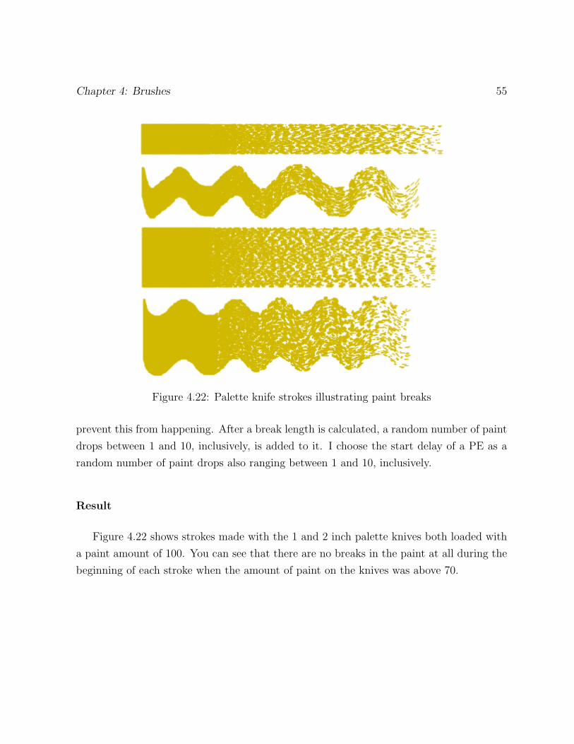
Chapter 4: Brushes 55
Figure 4.22: Palette knife strokes illustrating paint breaks
prevent this from happening. After a break length is calculated, a random number of paint
drops between 1 and 10, inclusively, is added to it. I choose the start delay of a PE as a
random number of paint drops also ranging between 1 and 10, inclusively.
Result
Figure 4.22 shows strokes made with the 1 and 2 inch palette knives both loaded with
a paint amount of 100. You can see that there are no breaks in the paint at all during the
beginning of each stroke when the amount of paint on the knives was above 70.

56 Automated Landscape Painting in the Style of Bob Ross
Figure 4.23: Paint scratched off the canvas using the corner of the palette knife
4.9.4 Scratching the Canvas
One of the ways that Bob Ross used the palette knife was to lightly scratch the canvas
with the corner to remove fine lines of paint. I implemented an alternate mode for the
palette knife to accommodate this technique. When in this mode, the knife only has one
PE located at its centre point and that PE is set to scratch mode. See Figure 4.23 for
an example of some paint scratching using a pressure of 30. Notice how the area in the
centre of all of the circular scratches has approached the original white colour of the canvas
more than the outer area. This was caused by overlapping scratches taking more and more
layers of paint off of the canvas.
4.9.5 More Examples
See Figure 4.24 for a few more examples of strokes painted using the palette knife.
Figure 4.25 shows a picture of two layers of palette knife strokes that were followed by
several transverse strokes using a dry palette knife.

Chapter 4: Brushes 57
Figure 4.24: More strokes using the palette knife
Figure 4.25: Layered and dry palette knife strokes

58 Automated Landscape Painting in the Style of Bob Ross
4.10 Conservation of Paint
The painting model comprising the paint brush and canvas layers does not conserve
paint on the canvas. For example, a small amount of paint deposited on the canvas from
a single stroke can be moved around using a dry brush to cover the entire surface of the
canvas. This anomaly arises because there is no concept of paint amount on the canvas,
only paint colour. A small amount of paint deposited by a stroke acts as an infinite pool
of paint from which a dry brush can move into surrounding areas of the canvas. While
conservation of paint is not required for the purpose of my painting model, it is a limitation
worth mentioning. Commercial applications PainterTM IX.5 and ArtRage 2 do not exhibit
conservation of paint either.
Implementing conservation of paint in my painting model would require storing the
amount of paint at each pixel location of the canvas, not just the paint colour. The paint
brushes would also need to have functionality to deposit and remove paint from different
locations on the canvas throughout each stroke. Emulating Bob Ross’s painting style does
not require a painting model that conserves paint on the canvas, so to limit its complexity,
I decided not to implement paint conservation.
4.11 Paintings
Aside from the paintings in the style of Bob Ross that will be presented in the following
chapters, Appendix C has several other paintings that were created using my paint brush
model. One of my colleagues, Jie Xu, was gracious enough to try out the brushes in my
application to paint his own painting — see Figure C.2 for his work. I also created my own
paintings, see Figures C.1 and C.3.

Chapter 5
Landscape Features
This chapter describes how I used the brushes from my brush model to paint all of the
landscape features that are included in one of Bob Ross’s paintings: Forest Hills. Some of
these features are included in many of his other paintings, while others are exclusive to this
particular painting. Most features require several different brush strokes and techniques to
paint. Different parts of features often require different kinds of brushes as well.
To automate the painting process of the landscape features, I examined video of Bob
Ross painting. During his videos, he identifies the brushes and paint colours that he uses,
the brush stroke techniques that he applies, and other important elements pertaining to
his particular style. I often needed to further analyze his painting techniques and style
beyond the descriptions that he gave during his videos to fully capture the way that he
painted his features in my application.
59
60 Automated Landscape Painting in the Style of Bob Ross
5.1 Painting Process
The process of painting each feature involves calculations that use a set of random
variables and specified parameters. The brush strokes that paint a feature are not recorded
in a macro of any kind — they are calculated on the fly as the feature is being painted.
Different paintings of the same feature with the same options never look exactly the same
because of randomness embedded in the brush model and stroke placement.
Since the brush strokes used to paint each feature are not pre-recorded, I can alter
certain parameters of each feature to make them look different. I made certain options
available for each feature that abstract the details of changing the specific values of feature
parameters so that the physical properties of features can be chosen easily by a user of this
layer. In the context of my application, a user of this layer can be a user of my application
or the landscape layout layer above this one, as shown in Figure 3.1.
Specific locations and sizes of brush strokes or parts of features will not be specified
in this chapter. There is something worth mentioning about sizes and locations, however.
Wherever possible, I randomized the locations and sizes of brush strokes or parts of features
so that features would have a naturally painted look. After all, Bob Ross does not paint
with the pinpoint accuracy and precision of a computer. To quote Bob Ross during one of
his shows, “We don’t make mistakes here, we just have happy accidents.” The mistakes
that Bob Ross made did not detract from his landscape features, they gave them a more
natural appearance. I try to simulate the carefree painting style of Bob Ross by injecting
randomness throughout every aspect of every procedure used to paint landscape features.
5.2 Reference Point
All of the strokes required to paint a feature are painted at locations on the canvas
that are relative to one reference point that is specified for each feature. Every landscape
feature has its own local model coordinates where the reference point is the origin. The
Chapter 5: Landscape Features 61
reference point of a feature could be directly in the centre of it or at some other important
position within the feature. A user of my application chooses the reference point of a
feature on the canvas by clicking on it at the desired location. The landscape layout layer
above this layer chooses the reference point for each feature to place them in locations on
the canvas that create a desired landscape.
5.3 Brush Strokes
Bob Ross used several different kinds of brush strokes to paint his landscape paintings.
I implemented all of the strokes that he used for one of his paintings, but these strokes are
certainly common enough that they are used in many of his other paintings as well. The
paint brushes layer offers two types of brush strokes: the line stroke and the stab. More
complex stroke trajectories are approximated with piecewise-linear paths, and painted as
a sequence of line strokes.
Each stroke is specified by a set of parameters. The common parameters among all of
the strokes are starting and ending brush rotations and pressures. Each stroke has a way
of specifying its location, but it is different for different kinds of strokes. A line stroke’s
location is specified by a start and end point on the canvas, for example.
5.3.1 Parabolic Stroke
One of the strokes that Bob Ross used has a relatively simple shape and is essentially a
second degree curve. I discovered that this type of stroke can be specified quite easily using
a section of a parabola. A parabolic stroke has three parameters that define its shape and
two parameters that specify its location. Two of the shape parameters specify the starting
and ending x values of the section of the parabola that will be used as the path of the
stroke. The other shape parameter is for adjusting the vertical stretch of the parabola.
Finally, the location of where the parabolic stroke will be painted on the canvas is specified

62 Automated Landscape Painting in the Style of Bob Ross
Figure 5.1: Illustration of a parabolic stroke
Figure 5.2: Illustration of a criss-cross stroke
by one point. See Figure 5.1 for an illustration of an example of a parabolic stroke.
5.3.2 Criss-Cross Stroke
A criss-cross stroke is a combination of two parabolic strokes painted one on top of the
other. The parabolic strokes always start from above and end on opposite sides of each
other. The order in which the parabolic strokes are painted does not matter, but Bob Ross
had a tendency to paint the one going from left to right first. A criss-stroke is defined by
the shape parameters of each of its parabolic strokes and a single point that specifies its
location. See Figure 5.2 for an illustration of a criss-cross stroke.
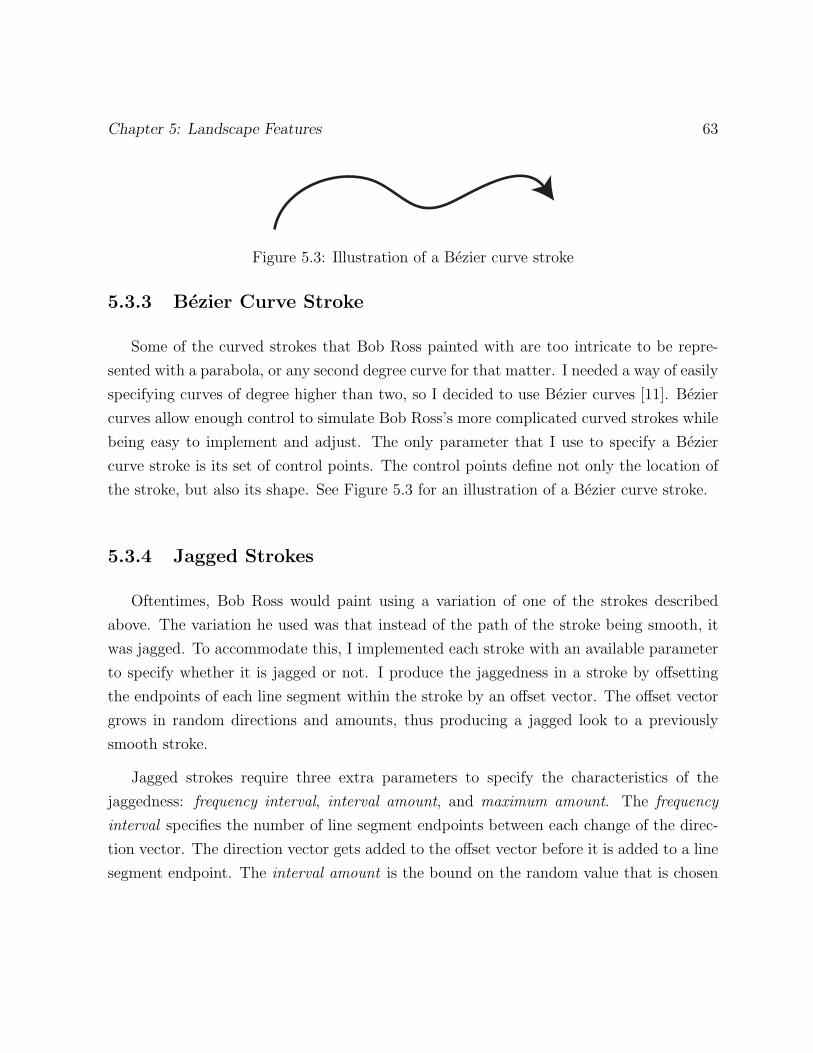
Chapter 5: Landscape Features 63
Figure 5.3: Illustration of a Bezier curve stroke
5.3.3 Bezier Curve Stroke
Some of the curved strokes that Bob Ross painted with are too intricate to be repre-
sented with a parabola, or any second degree curve for that matter. I needed a way of easily
specifying curves of degree higher than two, so I decided to use Bezier curves [11]. Bezier
curves allow enough control to simulate Bob Ross’s more complicated curved strokes while
being easy to implement and adjust. The only parameter that I use to specify a Bezier
curve stroke is its set of control points. The control points define not only the location of
the stroke, but also its shape. See Figure 5.3 for an illustration of a Bezier curve stroke.
5.3.4 Jagged Strokes
Oftentimes, Bob Ross would paint using a variation of one of the strokes described
above. The variation he used was that instead of the path of the stroke being smooth, it
was jagged. To accommodate this, I implemented each stroke with an available parameter
to specify whether it is jagged or not. I produce the jaggedness in a stroke by offsetting
the endpoints of each line segment within the stroke by an offset vector. The offset vector
grows in random directions and amounts, thus producing a jagged look to a previously
smooth stroke.
Jagged strokes require three extra parameters to specify the characteristics of the
jaggedness: frequency interval, interval amount, and maximum amount. The frequency
interval specifies the number of line segment endpoints between each change of the direc-
tion vector. The direction vector gets added to the offset vector before it is added to a line
segment endpoint. The interval amount is the bound on the random value that is chosen
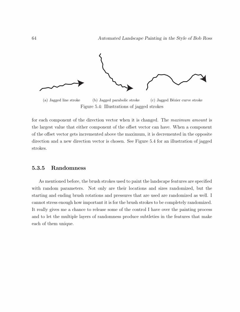
64 Automated Landscape Painting in the Style of Bob Ross
(a) Jagged line stroke (b) Jagged parabolic stroke (c) Jagged Bezier curve stroke
Figure 5.4: Illustrations of jagged strokes
for each component of the direction vector when it is changed. The maximum amount is
the largest value that either component of the offset vector can have. When a component
of the offset vector gets incremented above the maximum, it is decremented in the opposite
direction and a new direction vector is chosen. See Figure 5.4 for an illustration of jagged
strokes.
5.3.5 Randomness
As mentioned before, the brush strokes used to paint the landscape features are specified
with random parameters. Not only are their locations and sizes randomized, but the
starting and ending brush rotations and pressures that are used are randomized as well. I
cannot stress enough how important it is for the brush strokes to be completely randomized.
It really gives me a chance to release some of the control I have over the painting process
and to let the multiple layers of randomness produce subtleties in the features that make
each of them unique.

Chapter 5: Landscape Features 65
5.4 Forest Hills
Forest Hills is one of hundreds of landscapes painted by Bob Ross. It depicts a scene
where a lake divides a forest to reveal a view of a mountain range and several hills. Some of
the landscape features included in Forest Hills are common in many of his other paintings,
while others are not. For example, an evergreen tree is a common feature among Bob Ross
paintings, but a rocky bank is not.
The Forest Hills landscape includes a sky, mountains, a lake, hills, evergreen trees,
deciduous trees, rocky banks, and bushes — painted in that order. Only the mountain
feature is described in detail in this chapter. For the painting details of the other landscape
features, see Appendix A. Note that before any landscape features are painted, it is assumed
that there is a thin coat of white paint covering the entire canvas. This coat was always
painted by Bob Ross before he started a landscape painting to facilitate his wet-on-wet
technique for nearly all of the landscape features that he painted.
When specifying the paint colours used to paint all of the different landscape features,
I only describe them with words in this chapter. The exact RGB colour values for all of
the paint colours used for each part of every feature are listed in Appendix B.
5.5 Mountain Feature
Bob Ross painted mountains in almost all of his landscape paintings. He painted many
different kinds that varied in colour and shape depending on the location that he was trying
to convey. The mountains that he painted in Forest Hills are snow-covered and consist of
several distinct peaks. The predominant tool that he used to paint his mountains was
the two inch palette knife. He also used the two inch brush to blend the bottom of his
mountains. The reference point of the mountain feature is near its base, below the top of
the main peak.
There are two main stages to paint the mountain in Forest Hills. The first stage is to

66 Automated Landscape Painting in the Style of Bob Ross
Figure 5.5: Mountain undercoat
paint the underlying rock of the mountain and the second stage is to paint the snow. The
type of stroke that he used the most for the mountain feature is the parabolic stroke.
Because the mountains contain light-coloured snow, they are shown against a black
background. The painting process is unaffected since the paint on the palette knife does
not blend with paint on the canvas. When a landscape is generated automatically, the sky
is painted before the mountains, providing appropriate contrast for the snow.
5.5.1 Undercoat
See Figure 5.5 for a picture of a painted undercoat of the mountain feature. The
undercoat of the mountain in isolation reveals a lot of information about the geometry of
the mountain and each peak. The main peak, in the centre of the mountain, is the tallest.
The bottom of each peak lies roughly on the same horizontal line so that the bottom of
the mountain range is level.
Each peak is assigned a different, randomly chosen knife rotation angle. A peak’s knife
rotation is used while painting its parabolic strokes. The first parabolic stroke of each
peak starts at its top point and is painted downward and to the left. Each subsequent
parabolic stroke is painted in the same direction, but is offset downward and to the right
along a vector that is in the same direction as the knife rotation angle. The right side of
each peak is a straight line made by the start of all of the parabolic strokes used to paint
Chapter 5: Landscape Features 67
its undercoat. Each parabolic stroke is shorter in vertical length than the previous one so
that they all end at the same vertical level at the bottom line of the mountain. Note that
all of these parabolic strokes are smooth.
Aside from the smooth parabolic strokes that create the overall undercoat shape of
each peak, one other jagged parabolic stroke is painted on the left side of each peak. This
stroke is painted over top of the first smooth parabolic stroke of the peak. Its purpose is to
give each peak a little more character and randomness. To add further randomness to the
shapes of the peaks, two or three connected, jagged line strokes are painted at the top of
each peak. Three strokes are used for the main peak because of its size, and two are used
for the rest. The first stroke starts at a peak’s top point and can go upward or downward
randomly. The rest head mostly left and downward by random amounts, giving the top of
each peak a unique shape.
The undercoat of each peak is painted with a different colour. This is to give the effect
of aerial perspective. As the peaks go from left to right, they are supposed to be farther
and farther away from the viewer. To create this effect, the farther away a peak is, the
lighter its paint colour is. The undercoat of each peak is a shade of blue that is darkest
for the leftmost peak and lightest for the rightmost.
5.5.2 Undercoat Blending
Before any snow is painted on top of the undercoat, it is blended downward so that
the bottom line of the mountain becomes soft and fades slowly to the white on the canvas
below. See Figure 5.6 for a picture of the undercoat after it has been blended.
Most of the blending is done using line strokes with a dry two inch brush applied with
a heavy pressure. Two sets of blending strokes are painted for each peak. One set of five
strokes all go down and to the right, while another set of four strokes go down and to the
left. Each of the strokes start and end at the same vertical level. They start about half
way up the mountain and end well below the bottom. The set of strokes going right start

68 Automated Landscape Painting in the Style of Bob Ross
Figure 5.6: Mountain undercoat after blending
at the right side of each peak and successively progress left toward the centre. The set of
strokes going left start at the centre of each peak and progress to its left side. The strokes
going left have a brush rotation that is the same as the peak’s assigned knife rotation.
The strokes going right have a brush rotation of 180 degrees minus the knife rotation. The
first peak on the left gets two extra blending strokes that start at that peak’s centre and
go almost horizontally toward the left. I added these extra strokes to make the left side
of the first peak start more softly. The blending strokes are long enough that the strokes
of different peaks overlap each other. This is actually desirable and helps to produce a
nice shape at the bottom of the mountain when all of the undercoat blending has been
completed.
After the blending line strokes for each peak have been painted, four more blending
strokes are needed to soften the bottom of the mountain even further. The four strokes are
comprised of two sets of two strokes, where each set has a stroke going left and a stroke
going right. One set is painted below the other to cover all of the blended bottom of the
mountain. Each stroke is a shallow and horizontally symmetrical parabolic stroke that
spans the width of the entire mountain going from one side of the canvas to the other. A
medium amount of pressure and a vertical orientation of the two inch brush is used for
these blending strokes.
Chapter 5: Landscape Features 69
5.5.3 Ledges
A ledge is a small part of a peak that juts out and sometimes creates a small crevice
within a peak. Each peak has a certain number of ledges that add to its shape. The main
peak has three ledges, the peak to the left of the main peak has two ledges, the leftmost
peak and the peak on the right of the main peak have one ledge, and the rightmost peak
does not have any ledges. The locations of the top point of each ledge are chosen to be
below and slightly to the left of the top point of each peak. The knife rotation angle of
each ledge is chosen to be less than the rotation for the peak and each subsequent ledge
has a lower rotation angle. The exception to this is the last ledge of the main peak, its
rotation angle is made slightly higher to produce a good chance for a large crevice between
the last ledges. Since they are in front of each peak, the undercoat layer does not reveal
the structure of any of the ledges. They are mainly painted using the strokes for snow
shadow and illuminated snow.
5.5.4 Snow Paint Order
The snow on the peaks of the mountain feature is painted in order starting from the
farthest peak and ending at the closest. All of the snow on one peak is painted and blended
before the snow on the next peak is painted. Bob Ross explains that this ordering preserves
the sharp edges of snow that divide each peak, which helps reinforce the sense of depth
between them.
The ledges on a peak are painted from top to bottom since the highest ledge is perceived
to be farther away from the viewer than the lowest. A ledge is not painted to completion
like a peak; the snow shadow is painted for all of the ledges of a peak, and then the
illuminated snow is painted on each ledge.

70 Automated Landscape Painting in the Style of Bob Ross
Figure 5.7: Main peak with only snow shadows painted
5.5.5 Snow Shadows
Once the blending of the undercoat paint layer is complete, the snow on the mountain
is painted. The shadowed part of a peak is painted first. The paint colour I use for the
shadows varies between a light blue and a dark blue, depending on which peak or ledge I
am currently painting. In Figure 5.7, the two farthest peaks are complete, the two nearest
do not have any snow yet, and the main peak has had its snow shadows painted.
The first layer of snow shadows covers an entire peak with exactly the same strokes that
were used to paint its undercoat layer. After the undercoat is fully covered with shadow,
slightly jagged parabolic strokes are painted to represent each small ledge of the peak.
Each ledge is painted with a set of strokes that start from the ledge’s top point and are
directed downward and to the left. Each successive stroke of a ledge is offset downward
and to the right and is smaller in height than its predecessor. Before painting the shadow
strokes for each ledge, a stroke of paint underneath where each shadow stroke will go is
painted first. These strokes resemble the undercoat of the peak and are painted so that
each ledge will appear to have its own dark bedrock. The set of shadow strokes for a peak
are all painted with the same knife rotation as the undercoat of the peak. The shadow and
undercoat strokes for each ledge are all painted with the same knife rotation but different
ledges are painted with different rotations to add a varied and weathered look to the peaks.

Chapter 5: Landscape Features 71
Figure 5.8: Main peak with illuminated snow
The undercoat and shadow colours of the first ledge are slightly darker than the colours
used for its peak and each subsequent ledge is darker in colour to make it appear as if the
ledges are getting closer and closer to the viewer. The paint colours used for each layer of
shadows for a peak and its ledges is a lighter blue than what is used for their undercoat so
that the undercoat is visible through the paint breaks of the shadow paint. Each shadow
stroke for a peak and its ledges is painted with a paint amount that yields an appropriate
number of breaks in the paint.
5.5.6 Illuminated Snow
After the snow shadows for a peak are all completed, its illuminated snow is painted
next. The illuminated snow is painted in almost the same way for a peak as it is for all of
its ledges. The only difference is that the illuminated snow painted on a peak is a smooth
parabolic stroke whereas the snow painted on each ledge is a jagged parabolic stroke. The
paint colour used for the illuminated snow is a bright white. See Figure 5.8 for a picture
of the illuminated snow added to the main peak on top of its snow shadows.
The illuminated snow for a peak is painted with a smooth parabolic stroke that starts
at the top point of the peak and comes down and to the right forming a smooth snow
line on the right side of the peak. Actually, to acquire the desired amount of paint breaks
72 Automated Landscape Painting in the Style of Bob Ross
throughout the stroke, I painted the smooth parabolic stroke using three smaller strokes.
The three combined strokes follow one long trajectory; however, I load different amounts
of paint before each stroke so that the paint breaks in a more desirable pattern. Bob Ross
often reloaded paint on his palette knife within the illuminated snow strokes as well.
The rotation of the knife starts at the assigned knife angle for the peak and ends at a
nearly vertical orientation. This gives each peak’s illuminated snow strokes the appearance
of becoming thicker as they progress downward. Notice that the snow line for the main
peak is distinguishable from the blended snow of the peak to the right. This, along with
the difference in shadow colour, makes it look like the main peak is in front of the peak to
its right.
The illuminated snow strokes for each ledge are painted in a similar fashion to the peak
strokes except that the ledge parabolic strokes are jagged instead of smooth. This gives
each ledge a more random and rugged appearance. Each stroke starts at a ledge’s top
point and progresses downward and to the right. The starting and ending rotations are
again not the same, making each ledge stroke thicker at the bottom than at the top.
Each ledge also has a little stroke added to it to vary its shape at the top. Using the
one inch palette knife, a short stroke randomly placed around the top point of each ledge
is painted. This little stroke roughens the otherwise straight edge the top of each ledge
would have. The randomness of the location of this small stroke makes it highly visible for
some ledges and barely visible for others.
5.5.7 Snow Blending
After all of the illuminated snow is painted on a peak, one final step finishes it. Using
the two inch brush dry, a sequence of smooth parabolic strokes starting from well below the
peak and ending about half way up it blends all of the snow painted on the peak upward
and to the left. See Figure 5.9 for a picture of the completed main peak after the blending
strokes were painted over its snow.

Chapter 5: Landscape Features 73
Figure 5.9: Finished main peak with blended snow
Four sets of two strokes are used to blend the snow upward for the main peak, three
sets are used for the rest of the peaks. The first set of strokes start at the right of each peak
and each subsequent set starts left of the previous one. The shapes of the parabolic strokes
used to blend the snow are chosen to match the shape of the curved snow line on the right
side of each peak. None of the blending strokes should disrupt the snow line of a peak —
the first blending strokes should be painted right below it. The two strokes within each
set are painted at different pressures. The first stroke is painted at a high pressure and is
only painted near the bottom of the peak. The second stroke is painted with light pressure
and goes about half way up the peak. The starting brush rotation of each blending stroke
is the same as the ending knife rotation of the illuminated snow stroke for the peak. The
ending orientation of the brush for these strokes is nearly horizontal.
See Figure 5.10 for a picture of the completed mountain range. Since the left side
of the leftmost peak is exposed and is not covered by any another peaks, extra blending
strokes are used to blend it. Four sets of two strokes are used to blend the left side of the
first peak. They are directed upward and to the right. The sets of strokes start at the
bottom-centre of the first peak and are successively offset upward and to the left to blend
the entire left side of the peak. Similar pressures are used for these strokes as the blending
strokes that are used for the other peaks. The starting knife orientation for these strokes is
nearly horizontal and the ending rotation is the same as the assigned knife rotation angle

74 Automated Landscape Painting in the Style of Bob Ross
Figure 5.10: Completed mountain feature
for the peak.
5.5.8 Adjustable Attributes
There are two attributes of the mountain feature that can be adjusted. The first is the
size of the mountain. I made three sizes available: small, medium, and large. Different sizes
are easily implemented by adjusting the location of the top point of each peak accordingly.
The other option is how many peaks there are in the mountain range. I offer one, three,
or five peaks as presets in my application.
5.6 Other Features
Table 5.1 shows the figure numbers and appendix sections for all of the other landscape
features. The figure of a feature shows a sequence of pictures depicting its painting process,
while the appendix section of a feature presents the details of its painting process.

Chapter 5: Landscape Features 75
Table 5.1: Other feature figures and appendix sections
Feature Figure Appendix Section
Sky 5.11 A.1
Lake 5.12 A.2
Hills 5.13 A.3
Evergreen Tree 5.14 A.4
Deciduous Tree 5.15 A.5
Rocky Bank 5.16 A.6
Bush 5.17 A.7
Figure 5.11: Sky feature
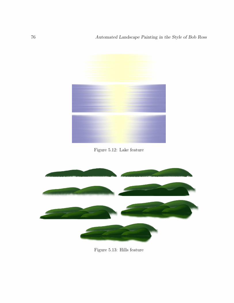
76 Automated Landscape Painting in the Style of Bob Ross
Figure 5.12: Lake feature
Figure 5.13: Hills feature
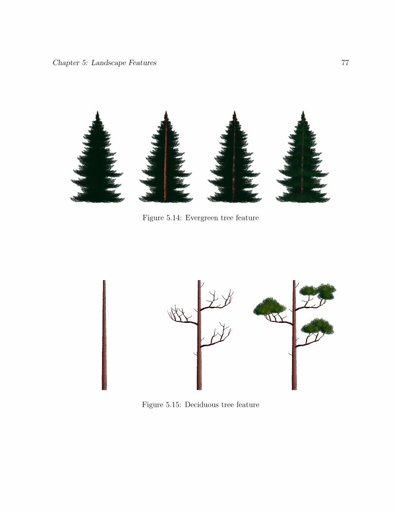
Chapter 5: Landscape Features 77
Figure 5.14: Evergreen tree feature
Figure 5.15: Deciduous tree feature
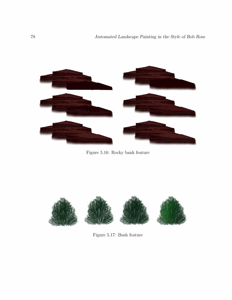
78 Automated Landscape Painting in the Style of Bob Ross
Figure 5.16: Rocky bank feature
Figure 5.17: Bush feature

Chapter 6
Landscape Layout
This chapter describes the final layer of my architecture, the landscape layout layer.
This layer is responsible for actually creating landscapes by automatically placing landscape
features at different locations on the canvas. Currently I have implemented the layout of
only one landscape, but it can easily be extended to paint other types of landscapes.
Recall that each landscape feature is painted relative to a reference point. The land-
scape features layer has an interface to set the reference points and adjustable attributes
of the features. A user of my application has direct access to the interface of the landscape
features layer. The reference point of a landscape feature is set by a user clicking on a lo-
cation on the canvas with the mouse; the adjustable attributes are chosen via menus. The
landscape layout layer uses the interface of the landscape features layer to automatically
create a landscape painting similar to Bob Ross’s Forest Hills.
The placement of each feature will be described in the order they are painted. While
describing where and how to place each landscape feature on the canvas, I will present a
figure of the updated painting including the most recent feature. Since the canvas is the
same colour as this page, it will not be visible until certain features are painted on it. Thus,
each figure will be displayed with a thin, black border so that the boundaries of the canvas
79

80 Automated Landscape Painting in the Style of Bob Ross
will always be visible. This modification will help show the layout of landscape features
relative to the canvas’s coordinate system. Recall that the canvas that Bob Ross uses for
his landscape paintings has a height of 18 inches and a width of 24 inches.
The layout of the landscape has several adjustable attributes. The most important one
that affects the placement and attributes of several different features is what side of the
canvas the deciduous tree will be painted on. Not only does this affect the placement of
the deciduous tree, but it affects the sky, evergreen trees, rocks, and bushes as well. Let
us assume that the deciduous trees will be painted on the left side of the canvas. Should
they be painted on the right, the reader must exchange left and right in the descriptions
that follow.
6.1 Sky Placement
The sky is usually the first feature that Bob Ross paints in his landscape paintings,
and Forest Hills is no exception. The centre of the sky is placed at the horizontal centre
of the canvas, 3.6 inches from the top. See Figure 6.1 for a picture of the canvas with the
sky feature painted on it.
The side of the sky that the cloud branch is painted on depends on the location of the
deciduous tree. When painted, the highest large branch of the deciduous tree takes up a
good portion of the sky. To balance the layout of the painting, the cloud branch is painted
on the other side of the sky that the large branch would be painted on. Otherwise, there
would be a fairly large empty space in the sky. In this case, the deciduous tree will be
painted on the left side of the canvas, so the cloud branch was painted on the right.

Chapter 6: Landscape Layout 81
Figure 6.1: Sky painted on the canvas

82 Automated Landscape Painting in the Style of Bob Ross
Figure 6.2: Mountain added to the painting
6.2 Mountain Placement
The mountain feature is also placed quite easily on the canvas. Recall that the reference
point of the mountain is underneath the top of the main peak near its base. Regardless of
its size, the mountain’s base is always placed at the same level on the canvas. This means
that larger mountains take up more of the sky rather than more of the lower half of the
canvas. The reference point of the mountain feature is placed at the horizontal centre of
the canvas and 10.5 inches from the top. See Figure 6.2 for a picture of the painting with
a mountain added to it. The mountain chosen for the painting is medium in size and has
Chapter 6: Landscape Layout 83
five peaks.
6.3 Lake Placement
Just as the sky serves as a backdrop for the upper half of the canvas, the lake feature
serves as a backdrop for the lower half. The lake is about 7 inches in height and as wide
as the entire canvas. The reference point of the lake is exactly at its centre. It is placed
at the horizontal centre of the canvas, 3.5 inches from the bottom. See Figure 6.3 for a
picture of the painting with a lake added to it. There are no adjustable attributes for the
lake feature.
6.4 Hills Placement
The hills are painted next. The reference point of the hills feature is at the bottom
edge of the start of the first row of hills. The start of a row of hills is on the left if the
hills are sloping downward toward the right and on the right if they are sloping downward
toward the left. The hills painted in this painting are sloping downward toward the left.
The reference point of the hills is placed in a location such that the first row of hills is
painted right on the top edge of the lake. It is placed in a different location depending on
what direction the hills are sloping downward in. Regardless of the downslope direction,
the hills are always placed 7 inches from the bottom of the canvas so that the first layer
rests at top of the lake. If the hills are sloping downward toward the left, as they are in
Figure 6.4, the reference point is placed exactly on the right edge of the canvas. If the
hills are sloping downward toward the right, the reference point is placed exactly on the
left edge of the canvas. Two rows of hills with an intermediate bumpiness level are used
in this painting.
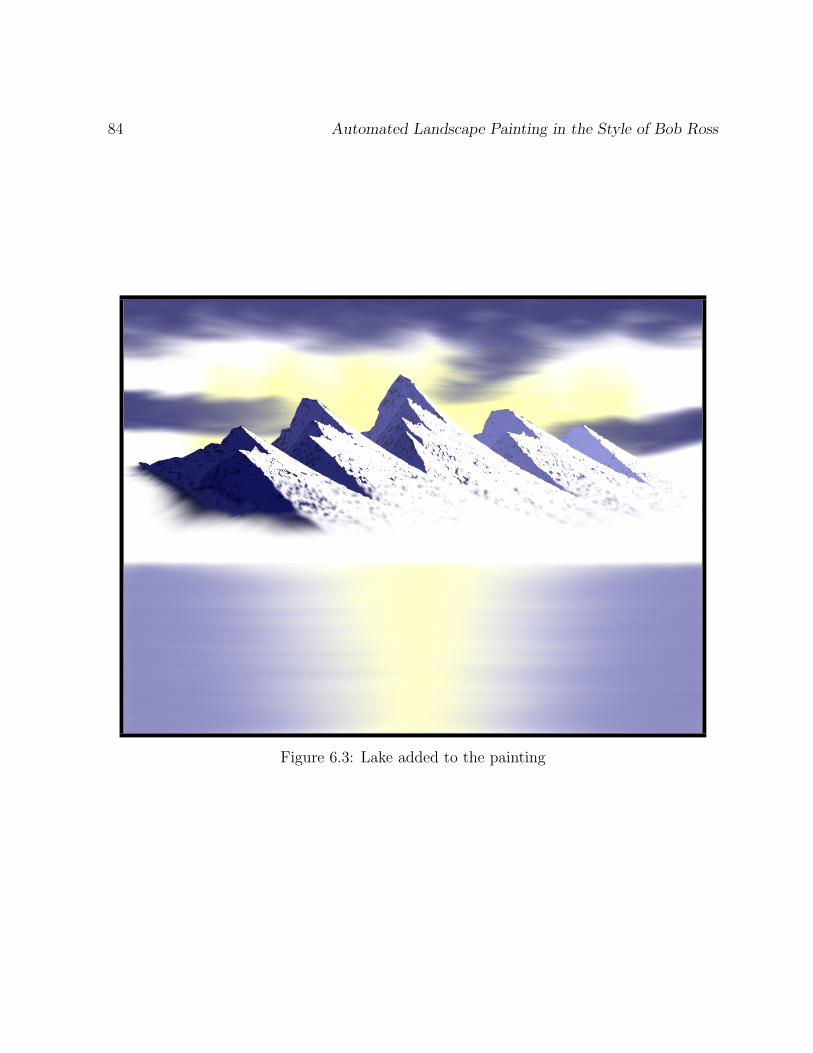
84 Automated Landscape Painting in the Style of Bob Ross
Figure 6.3: Lake added to the painting

Chapter 6: Landscape Layout 85
Figure 6.4: Hills added to the painting

86 Automated Landscape Painting in the Style of Bob Ross
Figure 6.5: Evergreen trees added to the painting
6.5 Evergreen Tree Placement
Several different evergreen trees are painted to create the forest in Forest Hills. There
are two sets of evergreens in the painting, one on each side of the canvas. The arrangement
of each set of evergreens depends on whether they are on the side of the canvas that has
the deciduous trees or not. All of the evergreens in Forest Hills have their leaves pointing
upward and the highlight side of their trunk is always oriented toward the centre of the
canvas. See Figure 6.5 for a picture of the painting with evergreen trees added to it. The
reference point of an evergreen tree is at the base of its trunk.

Chapter 6: Landscape Layout 87
6.5.1 On Deciduous Trees Side
The evergreen trees that are painted on the same side of the canvas as the deciduous
trees are all far away from the viewer. They serve as a backdrop for the deciduous trees
that will be painted in front of them. On this side of the canvas, three trees are painted.
The first tree, starting from the left, is large, while the other two, placed successively
toward the right, are medium-sized. The rocks that are placed on the deciduous tree side
of the canvas would block any reflections that these trees would make in the lake, so their
reflections are not painted.
The trees are placed in precise locations to achieve two goals. First, the large tree on
the left is placed so that none of the lake or the white empty space above the lake and to
the left of the mountain can be seen along the edge of the canvas beside the tree. This
tree must always be painted with some of its side off of the canvas. The other two trees
have similar goals of covering the area between the lake and the mountain. Second, the
tree closest to the centre of the canvas should be placed to the right as much as possible,
while not covering the tip of the second row of hills.
All three trees are placed at around the same vertical level, randomly between 3.2 and
3.5 inches from the bottom of the canvas. The three trees have their distances from the
left edge of the canvas chosen randomly within the intervals [0.4, 0.6], [1.75, 2.25], and
[3.5, 3.75]. The upper and lower bounds of the locations of each tree were chosen by visual
examination of how far each tree could be placed in either direction while adhering to the
goals mentioned above.
6.5.2 On Non-Deciduous Trees Side
The evergreen trees that are placed on the opposite side of the deciduous trees have a
different arrangement. On this side of the canvas, four trees are painted in total; two of
them are farther away from the viewer and the other two are closer. The reflections of the
evergreen trees on this side of the canvas are painted because they will be visible below

88 Automated Landscape Painting in the Style of Bob Ross
On the right In the middle On the left
Large tree [0.35, 0.85] [2.0, 2.5] [3.5, 4.0]
Medium tree farthest from water [2.0, 2.5] [0.35, 0.85] [0.35, 0.85]
Medium tree closest to water [3.5, 4.0] [4.0, 4.5] [1.5, 2.0]
Table 6.1: Evergreen tree locations on the non-deciduous trees side
the rocks.
The three trees closest to the side of the canvas consist of two medium-sized trees that
are far away and one large tree that is close. These trees are placed in a row with different
arrangements such that the large tree can either be on the left, on the right, or in the
middle of the two medium trees.
The arrangement where the large tree is in the middle of the two medium trees was
randomly chosen for the painting in Figure 6.5. Table 6.1 has the distance intervals, in
inches from the right side of the canvas, of each of the three trees in each arrangement.
The arrangements are identified by the location of the large tree relative to the medium
trees. The vertical locations of the trees are independent of the arrangement that they are
in. The large tree is always placed randomly between 5.0 and 5.5 inches from the bottom
of the canvas and the medium trees are placed randomly between 4.5 and 5.0 inches above
the bottom of the canvas.
The fourth tree on the left is always painted in the same way. It is a small tree that
is bent toward the centre of the canvas. Bob Ross includes a tree like this in many of his
landscape paintings that include evergreen trees. It is placed randomly between 4.25 and
4.5 inches above the bottom of the canvas and randomly between 5.5 and 6.0 inches away
from the right side of the canvas.
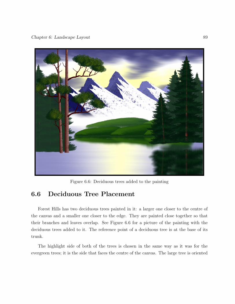
Chapter 6: Landscape Layout 89
Figure 6.6: Deciduous trees added to the painting
6.6 Deciduous Tree Placement
Forest Hills has two deciduous trees painted in it: a larger one closer to the centre of
the canvas and a smaller one closer to the edge. They are painted close together so that
their branches and leaves overlap. See Figure 6.6 for a picture of the painting with the
deciduous trees added to it. The reference point of a deciduous tree is at the base of its
trunk.
The highlight side of both of the trees is chosen in the same way as it was for the
evergreen trees; it is the side that faces the centre of the canvas. The large tree is oriented
90 Automated Landscape Painting in the Style of Bob Ross
vertically while the small tree is bent away from it. The side of the large tree with two
large branches faces the centre of the canvas. As mentioned before, the highest large
branch of the large tree covers a good portion of the sky across the canvas centre from the
cloud branch. To balance the layout of the two deciduous trees, the small tree has its two
medium branches on the opposite side of the large tree. This causes a portion of the lower
part of the evergreen trees in the background as well as the part of the sky near the corner
of the canvas to be covered by a few deciduous tree leaves. Also, the leaves of the branch
on the other side of the small tree have a good chance of covering the trunk of the large
tree between its two large branches, which would otherwise be fully exposed. The colour
of the leaves is dark green and their highlight is light yellow.
Both deciduous trees are placed randomly between 2.75 and 3.0 inches above the bottom
edge of the canvas. The large tree is placed randomly between 4.25 and 4.5 inches away
from the side of the canvas and the small tree is placed randomly between 3.75 and 4.0
inches away from the side of the canvas.
6.7 Rocky Bank Placement
After the deciduous trees have been painted, two rocky banks are added to the painting,
one underneath each set of trees. See Figure 6.7 for a picture of the painting with rocky
banks added to it. The reference point of the rocky bank feature is at its top near its
horizontal centre.
6.7.1 On Deciduous Tree Side
The rocky bank painted under the deciduous trees should start at their base and con-
tinue on past the bottom of the canvas. To achieve this, five rocks are used for the bank.
The rocks in this bank are set to recede slowly away from the water. The sloping scheme
among the rocks of this bank is set to progress from up or flat to down. Finally, the loca-

Chapter 6: Landscape Layout 91
Figure 6.7: Rocky banks added to the painting
92 Automated Landscape Painting in the Style of Bob Ross
tion of the water is set appropriately depending on which side of the canvas the rocks are
painted on.
The rocky bank on the same side of the canvas as the deciduous trees is placed randomly
between 4.0 and 4.25 inches from the side of the canvas and randomly between 3.1 and 3.4
inches from the bottom, inclusively. The location range is small because the rocky bank
has to overlap the bottom of the trees, extend past the bottom of the canvas, and leave a
minimum amount of space between it and the side of the canvas.
6.7.2 On Non-Deciduous Tree Side
The rocky bank painted on the other side of the deciduous trees starts at the base of the
evergreens and ends well above the bottom of the canvas. This is to show off the reflections
of the evergreens painted on the lake. Only three rocks are used for this bank. The rocks
in this bank are set to recede away from the water normally and to slope downward. Rocks
that have a downward slope are larger, and large rocks are needed under these evergreens
to cover the space between them and their reflections on the lake. The location of the
water is set appropriately for the rocky bank on this side as well.
The rocky bank on the opposite side of the canvas as the deciduous trees is placed
randomly between 5.1 and 5.4 inches from the side of the canvas and randomly between
4.1 and 4.4 inches from the bottom. There is not much leeway with this rocky bank
either. It has to cover the space between the trees and their reflections, leave enough space
underneath it to show off the reflections, and leave a small amount of space between it and
the side of the canvas.
6.8 Bush Placement
The bush is the final landscape feature to be painted in Forest Hills. Several bushes
of different sizes, orientations, and colours are painted on top of each rocky bank to finish

Chapter 6: Landscape Layout 93
Figure 6.8: Finished painting with bushes
the painting. See Figure 6.8 for a picture of the finished painting with bushes. Recall that
the reference point of a bush is at its horizontal centre near the bottom of its leaves.
The bushes not only have an artistic purpose, but a functional one as well. The bushes
need to be placed in such a way that any water that is visible below the evergreen trees
and above a rocky bank will be covered up. This goal restricts the amount of randomness
that can be used when placing bushes. Another restriction arises from the fact that each
bush must be placed on the top surface of a rock in a bank. If a bush is placed too far
away from the bank it looks like it is floating in the air above the water. Painted from the
same reference point, two rocky banks can randomly have rocks of different shapes and at

94 Automated Landscape Painting in the Style of Bob Ross
different locations, so the bushes must be constrained within an area that is assured to be
on top of any rock configuration.
There are two areas of bushes in the painting, one on top of each rocky bank. Each
area of bushes is painted in rows in order from top to bottom. The bushes within a row
are painted in order from the shore to the canvas edge. This paint order minimizes the
occlusion of highlights of some bushes by dark areas of others. This was the same concern
in painting the leaves on the deciduous tree. As with the trees, the bush highlights always
face toward the centre of the canvas.
The location of each bush in the first row of each area is randomized by up to ±0.1
inches in both the horizontal and vertical directions. The bushes in the rest of the rows are
randomized by up to ±0.2 inches in both the horizontal and vertical directions. The first
row of bushes is important for covering up the interface between the bottoms of the trees
and the water and rocks, so creating a gap between bushes in the first row is undesirable.
6.8.1 On Deciduous Tree Side
The bushes on the same side of the canvas as the deciduous trees are painted in either
three or four rows, chosen randomly. The bushes in the first row are painted with the dark
green leaf colour and the green highlight colour. The bushes in the remaining rows are
painted with the yellowish green leaf colour and the light yellowish green highlight colour.
The first row of bushes is painted 3.5 inches above the bottom of the canvas and each
subsequent row is painted 0.8 inches below the previous one. The bushes within a row are
painted approximately 1.5 inches apart starting from the bush closest to the side of the
canvas.
There are four bushes in the first row. The sizes of the bushes are randomly either
medium or large, except for the bush closest to the lake — it is always medium-sized. All
of the bushes in the first row are oriented straight up. The bushes are positioned so that
the one closest to the side of the canvas is right at its edge. The second row has three
Chapter 6: Landscape Layout 95
bushes. The sizes of the bushes are randomly either medium or large, except for the bush
closest to the lake, it is randomly small or small and flat. All of the bushes in the second
row are oriented straight up except for the one closest to the lake, which is bent toward
the lake. The bushes are positioned so that the one closest to the side of the canvas is 0.15
inches away from the edge. The third row has two bushes. The bush closest to the lake
is randomly small or small and flat and is bent toward the lake. The other bush is always
medium sized and straight up. The bushes are positioned so that the one closest to the
side of the canvas is 0.5 inches away from the edge. The fourth row only has one bush and
randomly appears half the time. The single bush is always small and flat with a straight
orientation. It is painted 1.25 inches from the side of the canvas.
6.8.2 On Non-Deciduous Tree Side
The bushes on the opposite side of the canvas as the deciduous trees are painted in
three rows. The bushes in the first row are painted with the dark green leaf colour and
the green highlight colour, except for the bush closest to the water, it is painted with the
green leaf colour and the light green highlight colour. The bushes in the rest of the rows
are painted with the yellow leaf colour and the light yellow highlight colour. The first row
of bushes is painted 4.5 inches above the bottom of the canvas and each subsequent row is
painted 0.5 inches below the previous one. The bushes within a row in this area are also
painted approximately 1.5 inches apart starting from the bush closest to the side of the
canvas.
There are five bushes in the first row. The sizes of the bushes are randomly either
medium or large, except for the bush closest to the lake, it is always small. All of the
bushes in the first row are oriented straight up. The bushes are positioned so that the one
closest to the side of the canvas is right on the edge. The second row has three bushes.
The sizes of the bushes are randomly either medium or large, except for the bush closest
to the lake, it is randomly small or small and flat. All of the bushes in the second row
are oriented straight up except for the one closest to the lake, which is bent toward the
96 Automated Landscape Painting in the Style of Bob Ross
lake. The bushes are positioned so that the one closest to the side of the canvas is 0.5
inches away from the edge. The third row has two bushes. The bush closest to the lake is
randomly small or small and flat and is bent toward the lake. The other bush is randomly
medium or small and straight up. The bushes are positioned so that the one closest to the
side of the canvas is 1.25 inches away from the edge.
6.9 Other Paintings
See Figure 6.9 for a picture of another automatically generated landscape painting. The
main difference between this painting and the previous one is the side of the canvas that
the deciduous tree is on. Notice that the cloud branch is painted on the opposite side to
balance out the sky. Also notice that the highlight side of all of the appropriate features
was painted accordingly. There are three other major differences between this painting and
the previous one. Firstly, the mountain is large instead of medium. Secondly, the hills have
three layers instead of two and were painted with a high lumpiness level instead of medium.
Finally, the arrangement of the evergreen trees on the opposite side of the deciduous trees
is different so that the large tree up close is at the edge of the canvas instead of being in
between the two medium trees far away.
Other, more subtle differences can be found within each and every feature because they
were all painted with many layers of inherent randomness, from the high level decisions
of placement and shape all the way down to the individual painting entities of each brush
stroke. See Figure 6.10 for a picture of four finished paintings with the same landscape
layout attributes. Even though each painting has the same arrangement of landscape
features, they look different because of the randomness within each individual feature.
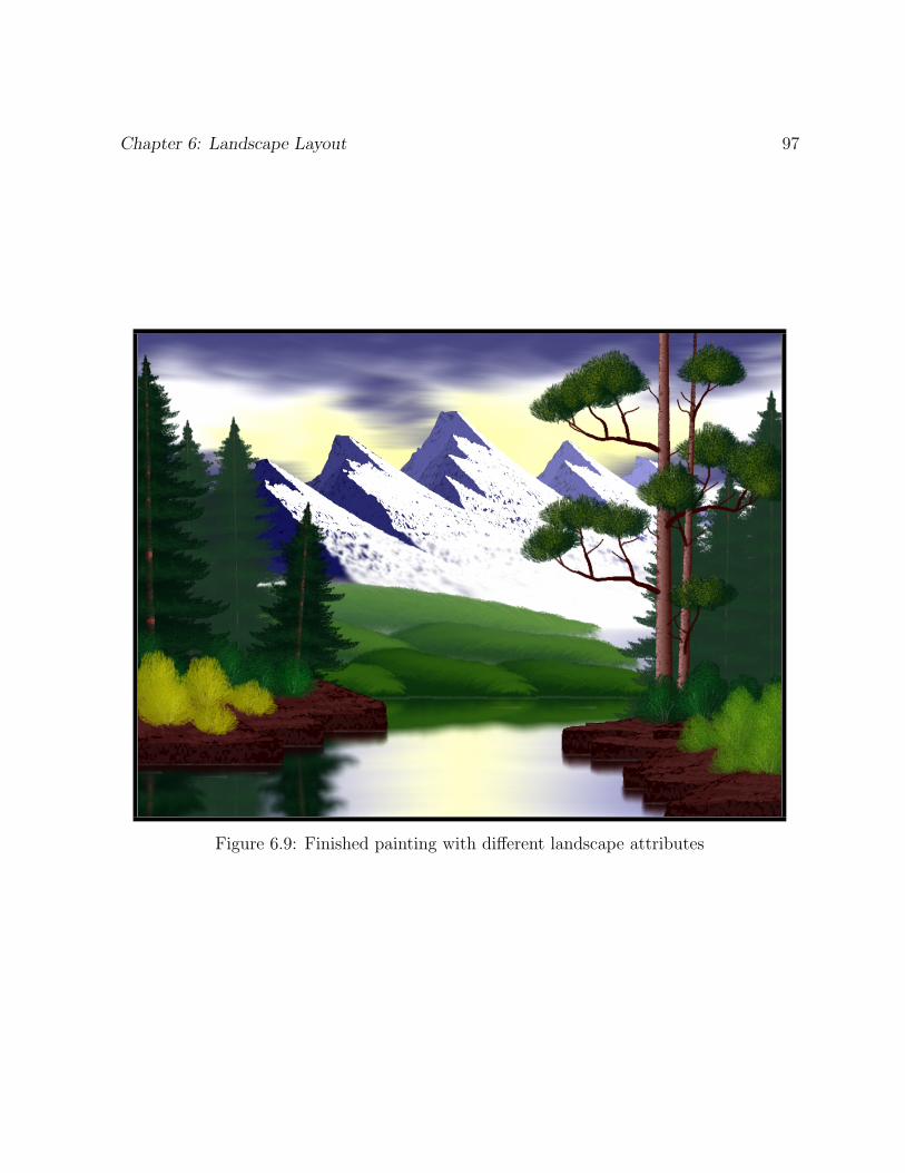
Chapter 6: Landscape Layout 97
Figure 6.9: Finished painting with different landscape attributes
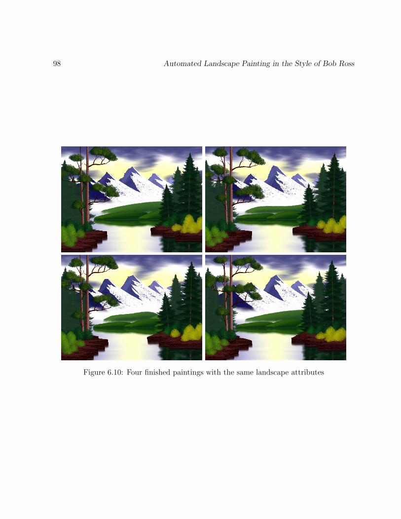
98 Automated Landscape Painting in the Style of Bob Ross
Figure 6.10: Four finished paintings with the same landscape attributes
Chapter 7
Conclusion
This chapter concludes my thesis by summarizing its results. I also discuss various
limitations and describe future work that can extend or improve upon what I have accom-
plished thus far.
7.1 Results
I have presented a way of automatically generating a landscape painting in the artistic
style of Bob Ross. My application can paint one of his landscape paintings, Forest Hills,
from start to finish, with one click of the mouse. The entire process of painting landscape
features at special locations across an empty canvas using different kinds of his brushes
and brush strokes is completely automated.
99
100 Automated Landscape Painting in the Style of Bob Ross
7.1.1 Painting Model
Working together, the canvas and brush layers of my software architecture provide a
simple, yet effective and versatile, painting model.
My painting model is simple relative to most painting models published in the litera-
ture. For the amount of functionality and quality of effects that it provides, its simplicity
is almost surprising. No 3D physical modelling of a brush is performed, no fluid dynamics
of paint are calculated, no advanced rendering techniques are used, and no hardware accel-
eration is employed. The brushes of my painting model can be used at interactive speeds
on an average computer by today’s standards.
My painting model is effective because it achieves one of its most important goals —
accommodating the painting effects produced from Bob Ross’s wet-on-wet technique. The
effect of paint blending is integral to reproducing the essence of a Bob Ross painting.
My painting model handles the mixing of paints with different colours correctly. It also
facilitates moving different amounts of existing paint on the canvas around using a dry
brush applied at different pressures.
The versatility of my painting model is shown by its ability to model six different kinds
of Bob Ross’s brushes. The brushes have a variety of shapes and sizes, and include a
palette knife, which is not even a brush at all. Special uses of certain types of brushes,
including scratching paint off of the canvas using a palette knife and using only the corner
of the fan brush, are also handled by my model.
The brushes of my painting model are not tied to the Forest Hills painting. They
are made to paint any of the features in any of his paintings. To illustrate this, see
Figures C.4 and C.5 in Appendix C for two other Bob Ross paintings that I created, Winter
Evergreens and Surf’s Up. The trees in Winter Evergreens were painted automatically by
my application, but I manually painted every other feature myself using only the paint
brushes.

Chapter 7: Conclusion 101
7.1.2 Landscape Features
The process of painting each of the landscape features present in Bob Ross’s Forest
Hills painting is automated successfully. The brush strokes used to paint each feature are
not pre-recorded, they are calculated on the fly while a feature is being painted. Brush
strokes and parameters are randomized so that two paintings of the same feature never
look exactly the same. Many of the features also have adjustable attributes that alter the
way they are painted to produce a variety of different forms of the same feature.
7.1.3 Landscape Layout
Painted in special locations together on the canvas automatically, the landscape features
successfully come together to form a whole, cohesive landscape painting. Different aspects
of the layout can also be adjusted to get different versions of Forest Hills.
7.1.4 User Interface
The user interface of my application provides two important affordances. The first is
that every automated brush stroke is displayed and animated as it paints. While each
stroke is painted, all of the brush parameters used for the stroke are updated in the user
interface interactively. This allows a user of my application to see how a painting is created
using the tools provided by my application. They can learn about Bob Ross’s painting
style and how to use my application at the same time. This type of displayed, automated
painting, coupled with real-time updates of brush parameters could be useful for teaching
users how to use commercial painting applications. Showing techniques in terms of brush
strokes that can be used to paint an actual painting within an application itself could be
an invaluable tool for learning.
The other affordance that the user interface of my application offers is that its different
painting modes can be used interchangeably. That is, a painting can be comprised of au-

102 Automated Landscape Painting in the Style of Bob Ross
tomatically painted landscape features as well as manually painted features using only the
brushes. Figure C.4 is a good example of this combination. The paint brushes and auto-
mated landscape features can be used together to produce original artwork that imitates
the style of Bob Ross.
7.2 Critique
In this section I discuss the amount of work that would be involved in automating
another landscape painting, and how my automated painting compares to the real thing.
7.2.1 Automating the Painting of Another Landscape
Now that I have completed the automation of an entire landscape painting, I have
a good idea of the amount of work required to accomplish such a task. Assuming the
brush and canvas layers are complete and ready to use, if I were to automate the painting
of another one of Bob Ross’s landscapes, there are three steps that would need to be
completed.
Brush Strokes
The first step is to automate any new brush strokes that Bob Ross used to paint the
landscape. This step is in the middle of the three in terms of difficulty. Once a suitable
mathematical representation for the brush stroke is found, it is not that hard to implement
the automation of the stroke with different shape and size parameters.

Chapter 7: Conclusion 103
Landscape Features
The second step is to automate the painting of the features that are included in the
new landscape. Of the three steps, this one is by far the most difficult to implement.
Not only does it require thought about how to mathematically choose the shapes, sizes,
and locations of all of the brush strokes used to paint the feature, but the fine-tuning
of brush and stroke parameters needed to finish and polish the painting of the feature is
time-consuming. There are two reasons why the fine-tuning process takes so long.
The first is that it is hard to choose the amount of randomness required to ensure that
the feature does not look the same every time it is automatically painted. A balance must
be found so that the randomness is enough to differentiate multiple paintings of the same
feature with the same attributes, but not so much that control over specific aspects of
the feature are lost. There are many facets of randomness that have to work together to
produce a landscape feature. Not only are the shapes, sizes, and locations of the brush
strokes randomized, but the orientations of the brush, the amount of paint loaded before
certain strokes, the applied pressures, and the stab offsets and directions are all randomized
as well.
The second reason why fine-tuning the implementation of a feature takes so much time
is because I have to translate what Bob Ross explains or demonstrates in his videos to
actual numbers to use in my program. For example, if he says to use a light pressure
for a brush stroke, I have to assign a number between 1 and 100 for that pressure in
my implementation. I also have to constantly experiment with the RGB values of paint
colours to try and match the different colours he produced by mixing paint together on his
palette during the show. Using a slightly incorrect paint colour can drastically reduce the
attractiveness and similarity of a landscape feature.
For soft aspects of landscape features including the clouds in the sky, the bottom of
the mountains, and the reflections on the water, the correct use of blending is critical. Not
only is the amount of applied pressure important for the brush strokes used for blending,
but the number of strokes is crucial as well. Blending is one of the hardest techniques and
104 Automated Landscape Painting in the Style of Bob Ross
required a lot of trial and error and fine-tuning to get close to the results that Bob Ross
produced. As a general rule for blending, it appeared that he would commonly use several
brush strokes over the same area that gradually decreased in pressure.
Another hardship arises during the implementation of a landscape feature because of
its adjustable attributes. Not only do I have to figure out a way to accommodate these
attributes using the geometrical models I have chosen for the feature, but all aspects of
randomization and the chosen stroke and brush parameters have to be specified in terms
of the different attributes so that the feature looks consistent across different combinations
of attribute parameters.
There are several aspects of Bob Ross’s painting technique and style that make automa-
tion difficult, but there is one important attribute of his paintings that makes automation
easier. The landscape features are painted independent of each other. None of the fea-
tures are painted with an assumption of how another features are painted. This makes
the development of the automation procedures a lot easier and allows the features to be
segregated into independent classes within the code of the landscape features layer.
One final thing to mention about the implementation of landscape features is that they
should be created with a consideration of how they fit into a given landscape. That is not
to say that they should only be able to fit into one kind of layout — they should definitely
be designed with flexibility. However, the motivation for what kind of adjustable attributes
landscape features should have certainly comes from examining how they reside in specific
landscapes.
Landscape Layout
Constructing the layout of a landscape is the easiest step in automating a landscape
painting. It only involves choosing appropriate locations and attributes for each feature to
produce a desired layout. There is some trial and error involved when choosing the random
range of locations for certain features, but it is minor compared to the fine-tuning required
for landscape features. The difficulty associated with creating the layout of a landscape
Chapter 7: Conclusion 105
depends on how well its features were implemented. If they are flexible enough in terms of
adjustable attributes, they will be able to fit into a variety of layouts much easier.
7.2.2 Automating the Painting of Another Landscape Feature
To explore the extendibility of the landscape features layer and to show that different
versions of the same feature can be used interchangeably in the same landscape, I auto-
mated the painting of another type of sky. The new type of sky has a different look than
the original sky in Forest Hills. It is a more conventional sky with a blue background and
fluffy clouds in the foreground.
Painting Process
The painting process for the new sky involves three stages. The first stage is to paint
a blue background. It is painted with a two inch brush using criss-cross strokes. The
strokes are painted in columns where wet strokes are followed by larger dry strokes used
for blending. The second stage is to paint the clouds. They are painted with a one inch
brush using circular strokes. Each of the clouds is painted using two different colours of
paint. A dark grey colour is used to paint the lower, shadow part of each cloud while a
white colour is used to paint the upper, lighter part. The last stage to finish the sky is to
blend the clouds in three phases. The first phase is used to blend the shadow and light
colours of paint together, while the last two phases are to soften the entire area of each
cloud. See Figure C.6 for a picture of Forest Hills with the new type of sky. Note that the
lake is painted without a sunny reflection to match this type of sky.
Analysis
Even though I had already automated the painting of eight other landscape features
beforehand, automating the new type of sky was still challenging. Painting the blue back-

106 Automated Landscape Painting in the Style of Bob Ross
ground for the sky was easy — the challenges lay in the clouds. Creating a new type
of stroke that follows a circular path was straightforward using my existing API. Using
the circular strokes to paint the initial stage of the clouds required a lot of fine-tuning to
balance desirable shapes and layout with as much randomness as possible.
The hardest aspect of painting the sky however, was the final stage of blending the
clouds. Since I was not used to blending with circular strokes, it was hard to find the right
combination of the number of strokes to use over a given area, the best sizes of strokes
to use, and how much pressure each stroke should be applied with in each of the three
phases of blending. Automating the blending of the clouds took a lot of experimentation
and refinement. This reaffirms my claim that blending is one of the hardest of Bob Ross’s
techniques to automate.
7.2.3 Comparison of my Automated Painting to the Real Thing
I think that someone familiar with Bob Ross’s painting style would recognize my au-
tomated painting of Forest Hills as one of Bob Ross’s paintings. Overall, my automated
Forest Hills looks like the actual Forest Hills painted by Bob Ross. When examined closely,
however, there are noticeable differences between my painting and his.
I think the main reason for the differences between my automated painting and the real
thing is due to my painting model. Painting with the brushes of my model does not look
exactly the same as when Bob Ross paints in real-life. I could have created my painting
model using complex physical simulations to accurately model the behaviour of real brushes
applying paint on a canvas, but it still would not have produced exactly the same results
that you see when Bob Ross is painting on his show. Bob Ross uses his own proprietary
brushes and paint. To obtain further realism using a physical simulation, details like the
density and material of the bristles on his brushes, the precise viscosity of the paint that he
uses, and the texture and absorbency of the particular canvas that he paints on would need
to be found. I do not only blame the approximations that I made to real-world physics
when building my painting model, but more the degree at which it mimics the particular
Chapter 7: Conclusion 107
media that Bob Ross uses. I am confident that with further fine-tuning and a few minor
adjustments, the results of my painting model can be brought closer to mimicking the
results of Bob Ross painting in real-life.
The painting model does not deserve all of the blame however, as the actual procedures
I use to automate Bob Ross’s painting style are approximated as well. As I mentioned
before, it is not easy to extract information from an instructional video and then encode it
into a form that my program can understand. Brush parameters such as pressure, loaded
paint amounts, and paint colours all have to be crudely approximated. Brush stroke
parameters and the geometry of each landscape feature are also approximated according
to what Bob Ross explains during his video and any other information I can extract from
visual inspection. Some of my automated features look more like his than others, and I
think that stems from the relative complexity inherent in the techniques that he used to
paint some his features, and not others. For example, in my opinion, the automated sky
in my painting matches the sky in his painting a lot more than my automated mountains
match his mountains.
One final point is that I am comparing my automated painting of Forest Hills to either
a picture of Bob Ross’s Forest Hills in his book or a video of it on his show. These media
do not convey subtle features found on the actual painting of Forest Hills. Looking at an
actual painting would reveal textures created from the shape of brush strokes and different
paint amounts that he used. I have not seen Forest Hills, or any actual Bob Ross painting,
in person, but I can guess that I would discover more differences between my automated
painting and his if I did.
It should not be a surprise that after many layers of approximation my automated
painting does not look exactly like Bob Ross’s painting. However, the goal of this thesis is
not to automatically reproduce a pixel-perfect imitation of a Bob Ross painting — it is to
capture his painting style, and I believe I have achieved that goal.

108 Automated Landscape Painting in the Style of Bob Ross
7.3 Limitations
There are a few limitations to my work that are worth mentioning. The most important
one is the number of landscape features that can be painted automatically. While some of
the automated landscape features, such as evergreen trees, appear in many of Bob Ross’s
paintings, it would have been nice to completely automate more than one of his landscape
paintings. However, as shown in Figures C.4 and C.5, my work can certainly be extended
to paint other Bob Ross paintings and the different concepts that I have presented to paint
the features of Forest Hills are applicable to other paintings of his.
Another limitation is that there is no interactive way to change brush parameters during
a stroke. For example, the pressure that a brush is painted with cannot be changed during
the path of a single stroke. The reason for this is purely interface related because my
automated strokes can certainly handle this functionality. While the mouse is being used
to draw a stroke, it cannot also be used to change the pressure that the brush is painted
with. A few keys on the keyboard could be assigned to increase or decrease the pressure
during a brush stroke or the starting and ending pressures for the next stroke could be
manually entered into the interface, but either of these solutions is clumsy. The best way
to accommodate this would be to take advantage of different dimensions of input that more
sophisticated devices tend to offer, like a pen tablet.
One last limitation worth mentioning pertains to the performance of my application.
Although painting with the brushes can be done at interactive speeds, automatically paint-
ing an entire landscape from start to finish takes about 15 minutes. It would be nice to be
able to have some kind of rendering mode where entire paintings are generated in a shorter
time.
Chapter 7: Conclusion 109
7.4 Future Work
One of the more obvious directions for future work is to automate more of the many
landscape features that Bob Ross painted in his other landscape paintings. If enough unique
features out of several different landscape paintings were automated, different combina-
tions of these features could be painted together to automatically create original landscape
paintings that would still be in the style of Bob Ross.
Along the lines of traditional NPR research, another extension to my work could be
to derive landscape layout from photos. By identifying the location and shapes of certain
features in a scene from a photo, landscape features could be painted by my application
to mimic the layout found in the photo.
To make the automated painting of landscape features more flexible, a scripting lan-
guage could be created to allow full control over brush stroke parameters. Scripts outlining
the sizes, shapes, and locations of brush strokes could be interpreted and subsequently ex-
ecuted by my application to paint new or customized versions of landscape features.
To explore areas of my painting model that can be improved upon, the results of my
brushes could be directly compared to the results of real brushes. Different types of strokes
could be examined and a better way of encoding brush parameters like paint amount and
pressure could be discovered.
The painting model of my application can be made more accessible by incorporating
support for pen tablet devices. Not only could this allow different brush parameters like
pressure to be changed during a stroke, but it would also make it far easier to paint than
it is with a mouse.
Finally, making use of programmable graphics hardware could provide my application
with a significant boost in performance. Since all of the brushes are composed of many
individual painting entities that interact with the canvas simultaneously throughout a
stroke, the parallelism offered by current GPUs could be leveraged to speed up the process
of painting in my application tremendously.


Appendix A
Landscape Feature Details
A.1 Sky Feature
The sky in Bob Ross’s Forest Hills painting consists of two major parts. First he paints
a light sunny area in the centre of the sky. Then he paints dark clouds that start from the
outside and encroach inward toward the centre. Only the two inch brush is used to paint
the sky, and he uses it both wet and dry. Since he makes heavy use of a dry brush, the
sky feature is a good example of how blending can be used for a real painting application.
The reference point for the sky feature is directly at its centre. The sky is painted mostly
using criss-cross strokes.
A.1.1 Sunny Area
The first part of the sky that is painted is the sunny area. Figure A.1 shows what the
sunny area of the sky looks like in isolation. The paint colour that I use for the sunny area
is a light yellow. The brush is oriented in a vertical direction for each of the strokes used.
111

112 Automated Landscape Painting in the Style of Bob Ross
Figure A.1: Sunny area of sky
I paint the sunny area in pieces by painting 12 sunny patches arranged in 2 rows and 6
columns. To have the sunny area arc upward toward the centre of the sky, each column
from the centre is painted at a successively lower level.
Each sunny patch is painted using several criss-cross strokes. Two criss-cross strokes
are used to apply the paint to the canvas while the brush is still wet. Four more strokes are
used afterwards when the brush is dry to blend out the patch. The wet criss-cross strokes
are painted above and below each other while the dry criss-cross strokes are painted in a
vertical row centred over where the wet strokes were. Heavy pressure is used during the
dry strokes to blend the paint as much as possible.
The pair of parabolic strokes used for each criss-cross stroke are different for when the
brush is wet and when its dry. The parabolic strokes used for the dry brush strokes are
wider than the strokes used while the brush is wet. This is so that the paint deposited
while the brush is wet can be blended with the surrounding white paint originally on the
canvas and any yellow paint from sunny patches that have already been painted.
The criss-cross strokes of each sunny patch are painted in a different order depending
on which row the patch is in. For the top row, the bottom criss-cross stroke is painted
first; for the the bottom row, the top criss-cross stroke is painted first. I did this because
the middle of the sunny area should be darker in colour than the top and bottom. The
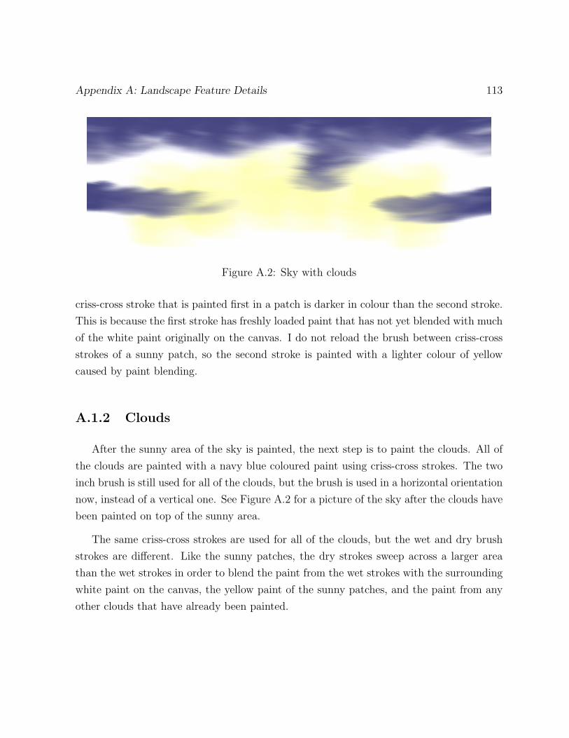
Appendix A: Landscape Feature Details 113
Figure A.2: Sky with clouds
criss-cross stroke that is painted first in a patch is darker in colour than the second stroke.
This is because the first stroke has freshly loaded paint that has not yet blended with much
of the white paint originally on the canvas. I do not reload the brush between criss-cross
strokes of a sunny patch, so the second stroke is painted with a lighter colour of yellow
caused by paint blending.
A.1.2 Clouds
After the sunny area of the sky is painted, the next step is to paint the clouds. All of
the clouds are painted with a navy blue coloured paint using criss-cross strokes. The two
inch brush is still used for all of the clouds, but the brush is used in a horizontal orientation
now, instead of a vertical one. See Figure A.2 for a picture of the sky after the clouds have
been painted on top of the sunny area.
The same criss-cross strokes are used for all of the clouds, but the wet and dry brush
strokes are different. Like the sunny patches, the dry strokes sweep across a larger area
than the wet strokes in order to blend the paint from the wet strokes with the surrounding
white paint on the canvas, the yellow paint of the sunny patches, and the paint from any
other clouds that have already been painted.

114 Automated Landscape Painting in the Style of Bob Ross
Cloud Branch
The cloud branch is the part of the clouds that comes down from the top of the sky and
bends toward the centre of the canvas. One of the options of the sky feature is to choose
which side of the horizontal centre the cloud branch is on, the left or the right. Whether
the branch is on the left or the right, its location is chosen within a random threshold.
To paint the cloud branch, four wet criss-cross strokes are painted in a line beginning
near the top of the sky and ending around its centre. Then, four dry criss-cross strokes are
painted at the same locations as the wet criss-cross strokes to blend them out.
The most important aspect of painting the cloud branch is to only load the brush with
dark blue paint at the start. This causes the paint on each successive stroke to blend with
the white and yellow paint on the canvas and become a lighter and lighter shade of blue
toward the end of the branch. Another important aspect of painting the cloud branch is
that it is painted before the top clouds and not after. I do this so that the many dry strokes
of the top clouds will merge the branch clouds and the top clouds together to create the
effect that the cloud branch seamlessly extends from the bottom of the top clouds.
Top Clouds
After the cloud branch is painted, the top clouds are next. I paint the clouds at the
top of the sky in columns of criss-cross strokes. The first column starts in the top-left of
the sky and each subsequent column is painted to the right of the previous one. In total,
12 columns of criss-cross strokes are painted to cover the width of the canvas.
Each column is comprised of either 3, 4, or 5 criss-cross strokes going down. The first
column on the left is assigned a random number between 3 and 5, inclusively. The rest
of the columns oscillate between 3 and 5, getting incremented or decremented by 1 each
time. The choice to increment or decrement the number of criss-cross strokes in successive
columns is made randomly. The oscillation of the number of criss-cross strokes produces a
wavy appearance at the bottom of the top clouds. The dry criss-cross strokes are painted

Appendix A: Landscape Feature Details 115
at the same locations as the wet criss-cross strokes, but only after the entire column is
painted, not after each wet criss-cross stroke.
The top of the top clouds should be darker than the bottom. I achieve this affect by
only loading paint on the brush at the start of each column. I used a similar technique
for the cloud branch. As each column of strokes progresses downward, the paint colour
turns from the original dark blue to a blended light blue. The paint amount I use at the
beginning of each column is dependant on the number of criss-cross strokes it has. The
more strokes a column has, the more paint is loaded on the brush before the column is
painted. The reason to use a paint amount that depends on the number of criss-cross
strokes rather than a constant amount is that I want the paint to run out during the last
criss-cross stroke of each column. If it runs out before the last stroke, no paint will be
deposited on the canvas during the last stroke. If it does not run out, the last stroke will
deposit too much paint on the canvas and will look too harsh. The bottom edge of the top
clouds should be fairly light in colour and end quite softly.
Side Clouds
Finally, two other clouds are painted on each side of the sky. The size and location of
each of these clouds depends on the location of the cloud branch. The cloud that is on the
same side of the sky as the cloud branch will be lower and shorter than the cloud on the
other side. This is to balance the layout of the sky and to ensure that the cloud branch
never touches a side cloud.
Each side cloud is painted with a series of criss-cross strokes that are located along the
path of two parabolas. The two parabolas of one side cloud are identical except for their
locations. One of the parabolas is slightly above and more toward the centre of the sky
horizontally than the other. The parabolas used for the shape of these clouds are quite
shallow.
I did not use different paint amounts for each cloud, despite one of them being longer
than the other. The reason for this is that I wanted the end of each cloud to look different.
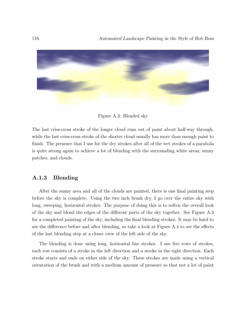
116 Automated Landscape Painting in the Style of Bob Ross
Figure A.3: Blended sky
The last criss-cross stroke of the longer cloud runs out of paint about half-way through,
while the last criss-cross stroke of the shorter cloud usually has more than enough paint to
finish. The pressure that I use for the dry strokes after all of the wet strokes of a parabola
is quite strong again to achieve a lot of blending with the surrounding white areas, sunny
patches, and clouds.
A.1.3 Blending
After the sunny area and all of the clouds are painted, there is one final painting step
before the sky is complete. Using the two inch brush dry, I go over the entire sky with
long, sweeping, horizontal strokes. The purpose of doing this is to soften the overall look
of the sky and blend the edges of the different parts of the sky together. See Figure A.3
for a completed painting of the sky, including the final blending strokes. It may be hard to
see the difference before and after blending, so take a look at Figure A.4 to see the effects
of the last blending step at a closer view of the left side of the sky.
The blending is done using long, horizontal line strokes. I use five rows of strokes,
each row consists of a stroke in the left direction and a stroke in the right direction. Each
stroke starts and ends on either side of the sky. These strokes are made using a vertical
orientation of the brush and with a medium amount of pressure so that not a lot of paint
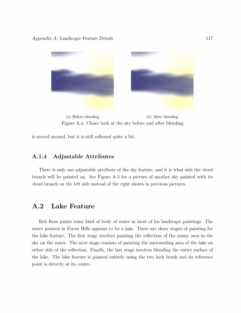
Appendix A: Landscape Feature Details 117
(a) Before blending (b) After blending
Figure A.4: Closer look at the sky before and after blending
is moved around, but it is still softened quite a bit.
A.1.4 Adjustable Attributes
There is only one adjustable attribute of the sky feature, and it is what side the cloud
branch will be painted on. See Figure A.5 for a picture of another sky painted with its
cloud branch on the left side instead of the right shown in previous pictures.
A.2 Lake Feature
Bob Ross paints some kind of body of water in most of his landscape paintings. The
water painted in Forest Hills appears to be a lake. There are three stages of painting for
the lake feature. The first stage involves painting the reflection of the sunny area in the
sky on the water. The next stage consists of painting the surrounding area of the lake on
either side of the reflection. Finally, the last stage involves blending the entire surface of
the lake. The lake feature is painted entirely using the two inch brush and its reference
point is directly at its centre.

118 Automated Landscape Painting in the Style of Bob Ross
Figure A.5: Sky with cloud branch on the left instead of the right
Figure A.6: Sunny reflection on the lake
A.2.1 Sunny Reflection
The sunny reflection on the lake is painted first. See Figure A.6 for a picture showing
the lake feature after only the sunny reflection has been painted.
Four rows of line strokes are used to paint the sunny reflection. Each row consists of
two line strokes that both start in the centre of the lake and end at different sides. A paint
amount is loaded on the brush before each stroke in every row such that each stroke runs
out of paint about half way to the side of the lake. As each stroke progresses outward, the
light yellow paint that is loaded on the brush gradually blends to the white colour already
on the canvas until the brush eventually runs out of paint. The four rows of strokes span
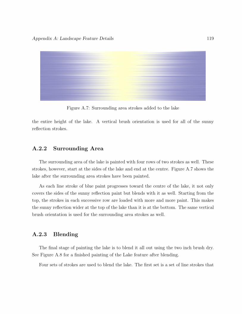
Appendix A: Landscape Feature Details 119
Figure A.7: Surrounding area strokes added to the lake
the entire height of the lake. A vertical brush orientation is used for all of the sunny
reflection strokes.
A.2.2 Surrounding Area
The surrounding area of the lake is painted with four rows of two strokes as well. These
strokes, however, start at the sides of the lake and end at the centre. Figure A.7 shows the
lake after the surrounding area strokes have been painted.
As each line stroke of blue paint progresses toward the centre of the lake, it not only
covers the sides of the sunny reflection paint but blends with it as well. Starting from the
top, the strokes in each successive row are loaded with more and more paint. This makes
the sunny reflection wider at the top of the lake than it is at the bottom. The same vertical
brush orientation is used for the surrounding area strokes as well.
A.2.3 Blending
The final stage of painting the lake is to blend it all out using the two inch brush dry.
See Figure A.8 for a finished painting of the Lake feature after blending.
Four sets of strokes are used to blend the lake. The first set is a set of line strokes that

120 Automated Landscape Painting in the Style of Bob Ross
Figure A.8: Blended lake
start from the top of the lake and end at the bottom. 15 of these strokes are used to cover
the entire width of the lake. A horizontal brush orientation and a heavy applied pressure
is used for this first set of strokes. The second set of blending strokes used to finish the
lake is comprised of five rows of horizontal strokes. Each row contains two strokes, one
starting on the left side of the lake and ending on the right and the other vice-versa. A
vertical brush orientation is used for this set of strokes and they are also applied with a
heavy pressure. The last two sets of blending strokes are identical to the first two sets
except that they are painted with a medium amount of pressure.
A.2.4 Adjustable Attributes
The only adjustable attribute of the lake feature is the sunny reflection. It can be
toggled on or off. If it is toggled off, a light blue colour is used to paint the centre of
the lake instead of a light yellow. See Figure A.9 for a picture of a lake with no sunny
reflection.

Appendix A: Landscape Feature Details 121
Figure A.9: Lake with no sunny reflection
A.3 Hills Feature
The hills in Forest Hills are mostly painted using the fan brush; however, the one and
two inch brushes, liner brush, and palette knife are used as well. The hills are arranged in
separate rows. Each row can contain up to three hills. The first step in painting a single
hill is to paint its undercoat. Afterwards, the highlights of a hill are painted on top of its
undercoat. The last step of painting a hill is to either paint a layer of mist near its bottom
if it is not in the front row; otherwise, if it is in the front row, the last step is to paint
reflections and water ripples in front of it on the lake. As usual with oil painting, the rows
of hills are painted in the order of farthest to closest.
A.3.1 Shapes
The shape of each hill within a row is specified using a Bezier curve [11]. The Bezier
curve can be one of two types. The first, and more simple, shape is a second degree curve
defined by three control points. The other, more intricate, shape is a fourth degree curve
defined by five control points. A hill with a second degree Bezier curve for its shape can
be described as having one mound. The second control point is placed much higher than
the first and the last control points to create a hill that is quite round. A hill with a fourth
degree Bezier curve for its shape can be described as having two mounds. The second
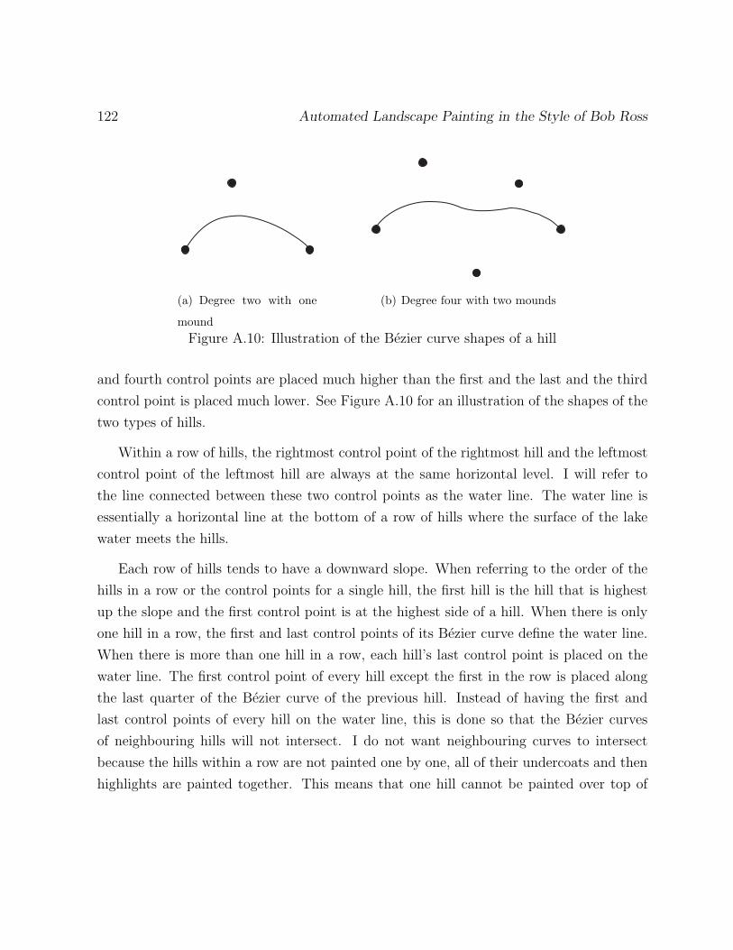
122 Automated Landscape Painting in the Style of Bob Ross
(a) Degree two with one
mound
(b) Degree four with two mounds
Figure A.10: Illustration of the Bezier curve shapes of a hill
and fourth control points are placed much higher than the first and the last and the third
control point is placed much lower. See Figure A.10 for an illustration of the shapes of the
two types of hills.
Within a row of hills, the rightmost control point of the rightmost hill and the leftmost
control point of the leftmost hill are always at the same horizontal level. I will refer to
the line connected between these two control points as the water line. The water line is
essentially a horizontal line at the bottom of a row of hills where the surface of the lake
water meets the hills.
Each row of hills tends to have a downward slope. When referring to the order of the
hills in a row or the control points for a single hill, the first hill is the hill that is highest
up the slope and the first control point is at the highest side of a hill. When there is only
one hill in a row, the first and last control points of its Bezier curve define the water line.
When there is more than one hill in a row, each hill’s last control point is placed on the
water line. The first control point of every hill except the first in the row is placed along
the last quarter of the Bezier curve of the previous hill. Instead of having the first and
last control points of every hill on the water line, this is done so that the Bezier curves
of neighbouring hills will not intersect. I do not want neighbouring curves to intersect
because the hills within a row are not painted one by one, all of their undercoats and then
highlights are painted together. This means that one hill cannot be painted over top of

Appendix A: Landscape Feature Details 123
Figure A.11: Undercoat of a first row of hills
another neighbouring hill that happens to be partly behind it. The hills of a single row
are painted in stages together rather than one by one so that the highlighting of each hill
in a row, described in detail later on, will look consistent.
The general width of each row of hills is pretty much the same. This means that the
more hills there are within a row, the smaller each hill will be. Also, the hills within a row
become successively smaller in height going in the direction of the downward slope of the
row. Since each row can have up to three hills and each hill within a row is a different size,
there are six different sizes of hills in total. Accounting for the fact that each size of hill
could have one or two mounds, there are 12 different shapes of hills in total. The number
of mounds of each hill is chosen randomly. The number of hills within a row is chosen
randomly with the constraint that the number of hills in a closer row must be more than
the number of hills in a row farther away. I do this because I do not want large hills to be
painted in front of small hills and have the small hills get covered up.
Each subsequent row of hills is painted below the previous one. Each row is also offset
from the previous one in the direction of the downward slope of the hills. So, if the hills
are sloping downward to the left, a row of hills will be painted below and slightly to the
left of the previous one. The reference point of the hills feature is at the location of the
first control point of the first hill within the first row.
A.3.2 Undercoat
The first step in painting a row of hills is to paint the undercoat layer. See Figure A.11
for a picture of the painted undercoat of the first row of a set of hills. The first hill on the
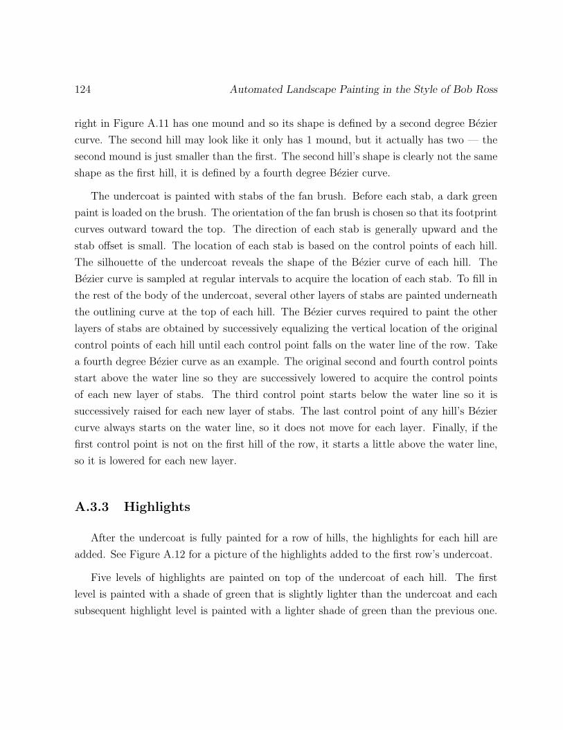
124 Automated Landscape Painting in the Style of Bob Ross
right in Figure A.11 has one mound and so its shape is defined by a second degree Bezier
curve. The second hill may look like it only has 1 mound, but it actually has two — the
second mound is just smaller than the first. The second hill’s shape is clearly not the same
shape as the first hill, it is defined by a fourth degree Bezier curve.
The undercoat is painted with stabs of the fan brush. Before each stab, a dark green
paint is loaded on the brush. The orientation of the fan brush is chosen so that its footprint
curves outward toward the top. The direction of each stab is generally upward and the
stab offset is small. The location of each stab is based on the control points of each hill.
The silhouette of the undercoat reveals the shape of the Bezier curve of each hill. The
Bezier curve is sampled at regular intervals to acquire the location of each stab. To fill in
the rest of the body of the undercoat, several other layers of stabs are painted underneath
the outlining curve at the top of each hill. The Bezier curves required to paint the other
layers of stabs are obtained by successively equalizing the vertical location of the original
control points of each hill until each control point falls on the water line of the row. Take
a fourth degree Bezier curve as an example. The original second and fourth control points
start above the water line so they are successively lowered to acquire the control points
of each new layer of stabs. The third control point starts below the water line so it is
successively raised for each new layer of stabs. The last control point of any hill’s Bezier
curve always starts on the water line, so it does not move for each layer. Finally, if the
first control point is not on the first hill of the row, it starts a little above the water line,
so it is lowered for each new layer.
A.3.3 Highlights
After the undercoat is fully painted for a row of hills, the highlights for each hill are
added. See Figure A.12 for a picture of the highlights added to the first row’s undercoat.
Five levels of highlights are painted on top of the undercoat of each hill. The first
level is painted with a shade of green that is slightly lighter than the undercoat and each
subsequent highlight level is painted with a lighter shade of green than the previous one.
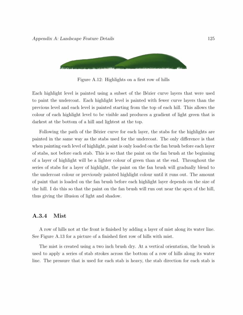
Appendix A: Landscape Feature Details 125
Figure A.12: Highlights on a first row of hills
Each highlight level is painted using a subset of the Bezier curve layers that were used
to paint the undercoat. Each highlight level is painted with fewer curve layers than the
previous level and each level is painted starting from the top of each hill. This allows the
colour of each highlight level to be visible and produces a gradient of light green that is
darkest at the bottom of a hill and lightest at the top.
Following the path of the Bezier curve for each layer, the stabs for the highlights are
painted in the same way as the stabs used for the undercoat. The only difference is that
when painting each level of highlight, paint is only loaded on the fan brush before each layer
of stabs, not before each stab. This is so that the paint on the fan brush at the beginning
of a layer of highlight will be a lighter colour of green than at the end. Throughout the
series of stabs for a layer of highlight, the paint on the fan brush will gradually blend to
the undercoat colour or previously painted highlight colour until it runs out. The amount
of paint that is loaded on the fan brush before each highlight layer depends on the size of
the hill. I do this so that the paint on the fan brush will run out near the apex of the hill,
thus giving the illusion of light and shadow.
A.3.4 Mist
A row of hills not at the front is finished by adding a layer of mist along its water line.
See Figure A.13 for a picture of a finished first row of hills with mist.
The mist is created using a two inch brush dry. At a vertical orientation, the brush is
used to apply a series of stab strokes across the bottom of a row of hills along its water
line. The pressure that is used for each stab is heavy, the stab direction for each stab is
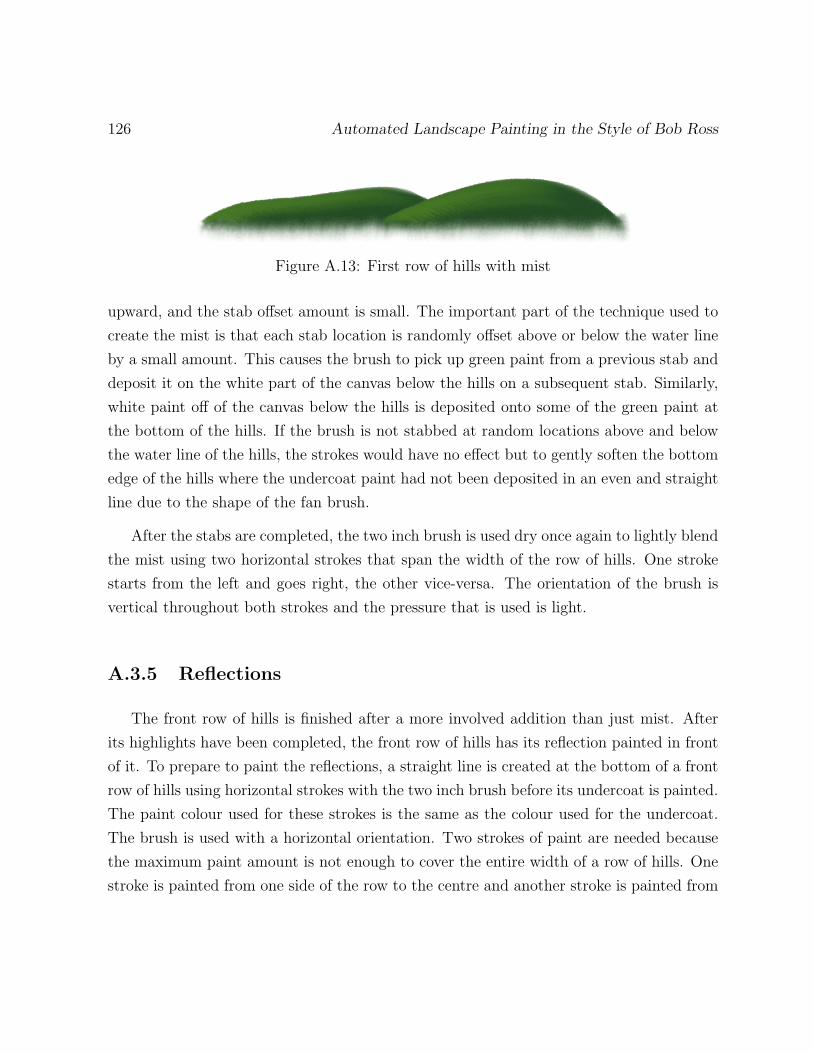
126 Automated Landscape Painting in the Style of Bob Ross
Figure A.13: First row of hills with mist
upward, and the stab offset amount is small. The important part of the technique used to
create the mist is that each stab location is randomly offset above or below the water line
by a small amount. This causes the brush to pick up green paint from a previous stab and
deposit it on the white part of the canvas below the hills on a subsequent stab. Similarly,
white paint off of the canvas below the hills is deposited onto some of the green paint at
the bottom of the hills. If the brush is not stabbed at random locations above and below
the water line of the hills, the strokes would have no effect but to gently soften the bottom
edge of the hills where the undercoat paint had not been deposited in an even and straight
line due to the shape of the fan brush.
After the stabs are completed, the two inch brush is used dry once again to lightly blend
the mist using two horizontal strokes that span the width of the row of hills. One stroke
starts from the left and goes right, the other vice-versa. The orientation of the brush is
vertical throughout both strokes and the pressure that is used is light.
A.3.5 Reflections
The front row of hills is finished after a more involved addition than just mist. After
its highlights have been completed, the front row of hills has its reflection painted in front
of it. To prepare to paint the reflections, a straight line is created at the bottom of a front
row of hills using horizontal strokes with the two inch brush before its undercoat is painted.
The paint colour used for these strokes is the same as the colour used for the undercoat.
The brush is used with a horizontal orientation. Two strokes of paint are needed because
the maximum paint amount is not enough to cover the entire width of a row of hills. One
stroke is painted from one side of the row to the centre and another stroke is painted from

Appendix A: Landscape Feature Details 127
Figure A.14: Undercoat of the front row of hills
Figure A.15: Front row of hills with highlights
the centre to the other side. The brush is loaded with the maximum paint amount before
each stroke. See Figure A.14 for a picture of the second (front) row of hills and notice the
straight bottom slightly below its water line. Figure A.15 shows the front row of hills with
highlights added to it. Notice that the front row is darker in colour than the back row.
Darker paint colours are used for each closer row of hills in order to produce the effect of
accumulating mist on rows of hills that are farther away. A similar technique is used for
the different peaks of the mountain feature.
I paint the reflections by painting the front row of hills again, except upside down.
Figure A.16 shows the hills after reflections of the front row have been painted. The
Figure A.16: Hills with reflections
128 Automated Landscape Painting in the Style of Bob Ross
reflections of the front row of hills are painted by following the exact same procedure as
the actual hills, but with a different set of control points. The original control points of
each hill in the front row are modified to produce reflections by reflecting the location of
each control point vertically across the water line of the row. Control points that were
above the water line are now below it by the same distance and control points that were
below the water line are now above it. Since each control point that was already on the
water line does not change after the reflection, the actual front row of hills and the reflected
front row of hills share the same water line. The reflections of the front row of hills should,
and do, start exactly at the water line. One last adjustment to the control points of the
reflected hill is to bring each of them a little closer to the water line so that the reflection
of the hills is not quite as large as the actual hills themselves.
Once the front row of hills has been painted again using the new set of control points,
they are blended using a two inch brush dry to make them actually look like a reflection.
The reflection is blended using four sets of strokes. The first set of strokes are vertical in
direction and start from the water line and go downward. A series of strokes are used so
that the entire width of the reflection is blended. A horizontal orientation of the brush
is used for these strokes with a heavy amount of pressure. The second set of strokes are
horizontal in direction. One of them is painted from left to right going across the entire
reflection and another going from right to left. These horizontal strokes are performed
with a vertical brush orientation and a high amount of pressure as well. The last two sets
of strokes are the same as the first two sets except that a light pressure is used instead.
A.3.6 Water Ripples
The final step to finish painting the hills feature is to add water ripples. Ripples are
painted at the water line and out in front of the hills. See Figure A.17 for a picture of a
finished set of hills with ripples in the water.
Each water ripple along the water line is painted using a combination of stabs with the
one inch palette knife and the one inch brush. At the location of a water ripple, one stab

Appendix A: Landscape Feature Details 129
Figure A.17: Finished hills with water ripples
with the knife in a horizontal orientation is made with a medium amount of paint. The
paint colour used is a grayish white. Then, a random number of stabs between 15 and 20,
inclusively, are made with the one inch brush dry at random locations around the ripple
with a light pressure. The direction of these stabs is pointing upward and the stab offset
used is a medium amount. The stabs with the dry brush are to soften and randomize the
stabs of the knife which would come out quite straight and sharp otherwise. The ripples
are painted in between control points that are on the water line. This means that they
start at the last control point of one hill and end at the last control point of a previous hill.
For the first hill however, both its end control points are on the water line so its ripples
would start and end at its first and last control points. To make it so that all of the ripples
are not painted on the same line for an entire row of hills, the first ripple of a hill starts
at the water line and each subsequent ripple is painted slightly above the previous ripple.
When the first ripple for the next hill is painted, it will be below the last ripple of the
previous hill. This slight modification to the ripple locations makes each hill within a row
look more distinct.
The ripples painted out in front of the hills are painted with the liner brush instead of
the palette knife. This is to give these water ripples a fading appearance at one side, as
the paint on the brush blends with the paint underneath as the line stroke progresses. The
amount of paint loaded onto the liner brush depends on how long the ripple is so that it
will run out toward the end. The number of ripples painted in front of the hills is either
two or three, chosen at random, and they each vary in location and length. Each ripple
line stroke is painted in the opposite direction of the downward slope direction of the hills.
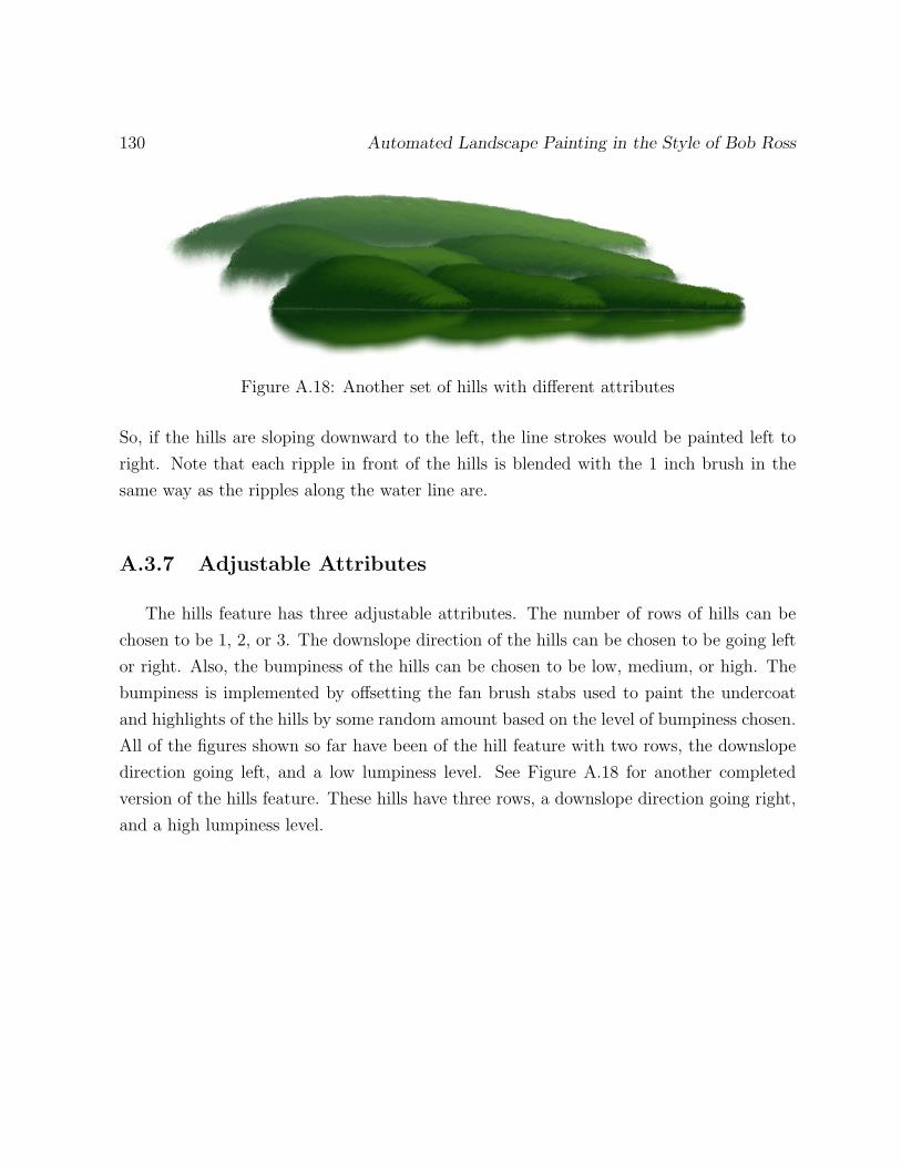
130 Automated Landscape Painting in the Style of Bob Ross
Figure A.18: Another set of hills with different attributes
So, if the hills are sloping downward to the left, the line strokes would be painted left to
right. Note that each ripple in front of the hills is blended with the 1 inch brush in the
same way as the ripples along the water line are.
A.3.7 Adjustable Attributes
The hills feature has three adjustable attributes. The number of rows of hills can be
chosen to be 1, 2, or 3. The downslope direction of the hills can be chosen to be going left
or right. Also, the bumpiness of the hills can be chosen to be low, medium, or high. The
bumpiness is implemented by offsetting the fan brush stabs used to paint the undercoat
and highlights of the hills by some random amount based on the level of bumpiness chosen.
All of the figures shown so far have been of the hill feature with two rows, the downslope
direction going left, and a low lumpiness level. See Figure A.18 for another completed
version of the hills feature. These hills have three rows, a downslope direction going right,
and a high lumpiness level.

Appendix A: Landscape Feature Details 131
A.4 Evergreen Tree Feature
The “happy” evergreen tree is a common feature among Bob Ross’s landscape paintings.
It appears in different sizes, colours, and layouts. The Forest Hills painting contains several
evergreen trees. Each tree is painted in four stages. First the undercoat of the leaves is
painted. Then the trunk of the tree is painted on top of the undercoat. The trunk is
then covered up with a few leaves that are of the same colour as the undercoat. Finally,
highlights are painted to bring out the green colour of the leaves. Some evergreen trees
are painted with a reflection, and so this would be the final step in painting a tree if it is
required. The fan brush, two inch palette knife, filbert brush, and two inch brush are all
used to paint an evergreen tree. The reference point of the evergreen tree feature is at the
bottom of the tree at the base of its trunk.
A.4.1 Leaf Stab Locations
The leaves of the evergreen tree are painted using stab strokes with the corner of the
fan brush. The leaves of the tree start out small at the top and progressively get bigger
as they reach the bottom. This is achieved with the fan brush by using a light pressure
for the stabs at the top of the tree and successively increasing the pressure used for each
lower level of stabs.
The leaves of a tree are painted in a series of levels, starting from the top of the tree.
The leaves in a single level are all painted with the same amount of pressure. Each level
has a certain number of rows of stabs. The number of rows for each level increases as they
get farther down the tree. Each row within a level is painted with a different number of
stabs. The top row of each level has the lowest number of stabs and the number of stabs
increases for each lower row within the level. The stabs within a row of any given level are
painted starting from the centre of the tree and going outward. A row in a level on the
left side of a tree would be painted right to left, and a row in a level on the right side of a
tree would be painted left to right. The stabs within a row are painted along a line that is

132 Automated Landscape Painting in the Style of Bob Ross
perpendicular to the tree line. The tree line is a line between the reference point of a tree
and its top point. The tree line is not always completely vertical since trees can be tilted
to the left or to the right.
The number of levels in a tree depends on the size of the tree. A large tree has more
levels than a smaller tree. The extra levels on a large tree have more rows and each row
has more leaves. A small tree has a subset of the level structure of a large tree. The top
half of a large tree, for example, will look similar to an entire small tree.
The level and row structure of leaves provides a good starting point to acquire the
locations of each stab required to paint the leaves of a tree. The right amount of randomness
needs to be introduced into this structure so that a tree looks organic, but not alien. Each
of the leaves are easily randomized by offsetting the starting location of each stab by a
slight amount. Too much randomness here can cause the tree to look strange. Another
way to make the tree more random is to randomize the number of stabs in each row by a
maximum of ±1. This provides great randomness in most occasions; however, when the
number of stabs in a row is decreased by 1 and then the number of stabs in the subsequent
row below gets increased by one, this part of the tree looks odd. The reason is that the row
below has three more stabs than the row above — two from the randomness and one from
the natural structure of each level where each subsequent row has one more stab than the
previous one. To fix this, I check to see if a row has more than 3 stabs than the previous
row above it after it has been randomized. If this is the case, a new random number to
adjust the stabs, either 0 or −1, is chosen for the row below.
After the all of the locations of the leaf stabs have been established, they are stored
and used to paint 4 of the 5 stages of the tree. The painting of the trunk of the tree
has nothing to do with the locations of its leaves. Note that the randomness of the stab
locations used to paint the leaves is required for the evergreen tree feature. One of the
reasons is to make a single tree look more organic. A more important reason, however, is
that several evergreen trees with the same attributes will be painted in the same landscape
painting. Without enough randomness, those trees would look too much alike, especially
if they are placed next to each other.
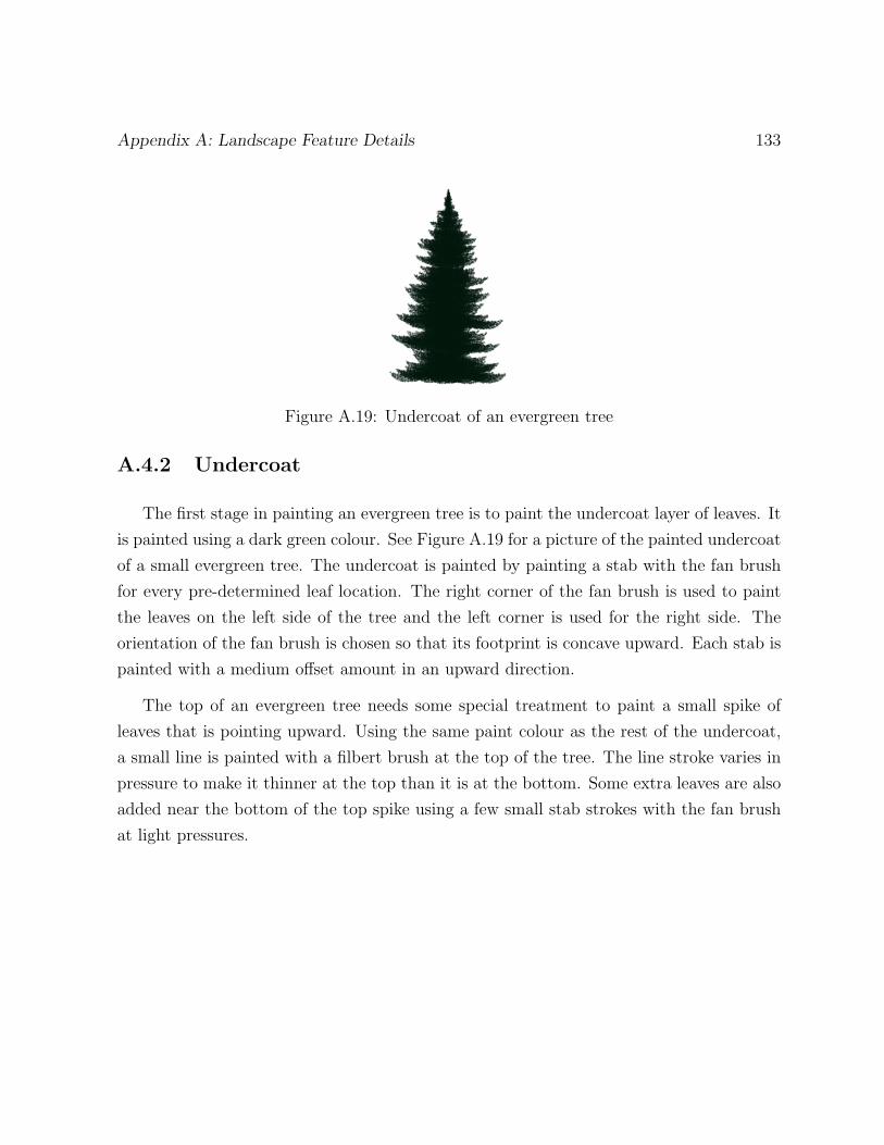
Appendix A: Landscape Feature Details 133
Figure A.19: Undercoat of an evergreen tree
A.4.2 Undercoat
The first stage in painting an evergreen tree is to paint the undercoat layer of leaves. It
is painted using a dark green colour. See Figure A.19 for a picture of the painted undercoat
of a small evergreen tree. The undercoat is painted by painting a stab with the fan brush
for every pre-determined leaf location. The right corner of the fan brush is used to paint
the leaves on the left side of the tree and the left corner is used for the right side. The
orientation of the fan brush is chosen so that its footprint is concave upward. Each stab is
painted with a medium offset amount in an upward direction.
The top of an evergreen tree needs some special treatment to paint a small spike of
leaves that is pointing upward. Using the same paint colour as the rest of the undercoat,
a small line is painted with a filbert brush at the top of the tree. The line stroke varies in
pressure to make it thinner at the top than it is at the bottom. Some extra leaves are also
added near the bottom of the top spike using a few small stab strokes with the fan brush
at light pressures.
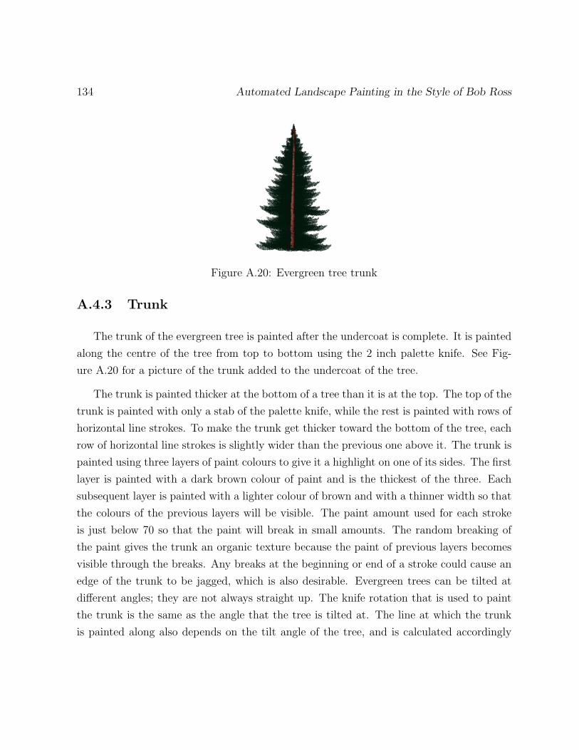
134 Automated Landscape Painting in the Style of Bob Ross
Figure A.20: Evergreen tree trunk
A.4.3 Trunk
The trunk of the evergreen tree is painted after the undercoat is complete. It is painted
along the centre of the tree from top to bottom using the 2 inch palette knife. See Fig-
ure A.20 for a picture of the trunk added to the undercoat of the tree.
The trunk is painted thicker at the bottom of a tree than it is at the top. The top of the
trunk is painted with only a stab of the palette knife, while the rest is painted with rows of
horizontal line strokes. To make the trunk get thicker toward the bottom of the tree, each
row of horizontal line strokes is slightly wider than the previous one above it. The trunk is
painted using three layers of paint colours to give it a highlight on one of its sides. The first
layer is painted with a dark brown colour of paint and is the thickest of the three. Each
subsequent layer is painted with a lighter colour of brown and with a thinner width so that
the colours of the previous layers will be visible. The paint amount used for each stroke
is just below 70 so that the paint will break in small amounts. The random breaking of
the paint gives the trunk an organic texture because the paint of previous layers becomes
visible through the breaks. Any breaks at the beginning or end of a stroke could cause an
edge of the trunk to be jagged, which is also desirable. Evergreen trees can be tilted at
different angles; they are not always straight up. The knife rotation that is used to paint
the trunk is the same as the angle that the tree is tilted at. The line at which the trunk
is painted along also depends on the tilt angle of the tree, and is calculated accordingly
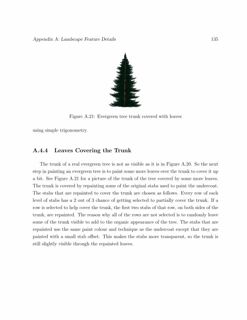
Appendix A: Landscape Feature Details 135
Figure A.21: Evergreen tree trunk covered with leaves
using simple trigonometry.
A.4.4 Leaves Covering the Trunk
The trunk of a real evergreen tree is not as visible as it is in Figure A.20. So the next
step in painting an evergreen tree is to paint some more leaves over the trunk to cover it up
a bit. See Figure A.21 for a picture of the trunk of the tree covered by some more leaves.
The trunk is covered by repainting some of the original stabs used to paint the undercoat.
The stabs that are repainted to cover the trunk are chosen as follows. Every row of each
level of stabs has a 2 out of 3 chance of getting selected to partially cover the trunk. If a
row is selected to help cover the trunk, the first two stabs of that row, on both sides of the
trunk, are repainted. The reason why all of the rows are not selected is to randomly leave
some of the trunk visible to add to the organic appearance of the tree. The stabs that are
repainted use the same paint colour and technique as the undercoat except that they are
painted with a small stab offset. This makes the stabs more transparent, so the trunk is
still slightly visible through the repainted leaves.

136 Automated Landscape Painting in the Style of Bob Ross
Figure A.22: Finished evergreen tree with highlights
A.4.5 Highlights
The final stage of painting the tree is to add highlights. The highlights are painted in
lighter shades of green than the undercoat is. See Figure A.22 for a picture of a finished
evergreen tree. The highlights are painted by repainting the bottom five rows of stabs of
each level of leaves with successively lighter shades of green. The lowest row is painted
with the lightest green and each row above is darker than the previous one so that the
highlights blend into the undercoat. If a level of leaves has less than five rows, highlights
are painted on all of the rows, but only the darkest highlight colours that can fit in the level
will be used. For example, if a level only has two rows, the two darkest highlight colours
will be painted on that level. Like the stabs used to cover the trunk, highlight stabs are
painted in the same way as the undercoat stabs except that the amount of offset that is
used is small.
A.4.6 Reflection
The option to paint a reflection of an evergreen tree is available. In some of Bob Ross’s
paintings, Forest Hills included, some trees have a reflection in the water and others do
not. This is only because of the chosen layout of the landscape. See Figure A.23 for a
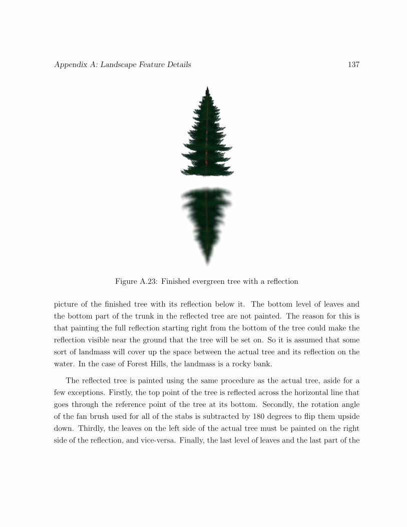
Appendix A: Landscape Feature Details 137
Figure A.23: Finished evergreen tree with a reflection
picture of the finished tree with its reflection below it. The bottom level of leaves and
the bottom part of the trunk in the reflected tree are not painted. The reason for this is
that painting the full reflection starting right from the bottom of the tree could make the
reflection visible near the ground that the tree will be set on. So it is assumed that some
sort of landmass will cover up the space between the actual tree and its reflection on the
water. In the case of Forest Hills, the landmass is a rocky bank.
The reflected tree is painted using the same procedure as the actual tree, aside for a
few exceptions. Firstly, the top point of the tree is reflected across the horizontal line that
goes through the reference point of the tree at its bottom. Secondly, the rotation angle
of the fan brush used for all of the stabs is subtracted by 180 degrees to flip them upside
down. Thirdly, the leaves on the left side of the actual tree must be painted on the right
side of the reflection, and vice-versa. Finally, the last level of leaves and the last part of the
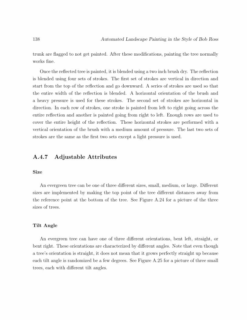
138 Automated Landscape Painting in the Style of Bob Ross
trunk are flagged to not get painted. After these modifications, painting the tree normally
works fine.
Once the reflected tree is painted, it is blended using a two inch brush dry. The reflection
is blended using four sets of strokes. The first set of strokes are vertical in direction and
start from the top of the reflection and go downward. A series of strokes are used so that
the entire width of the reflection is blended. A horizontal orientation of the brush and
a heavy pressure is used for these strokes. The second set of strokes are horizontal in
direction. In each row of strokes, one stroke is painted from left to right going across the
entire reflection and another is painted going from right to left. Enough rows are used to
cover the entire height of the reflection. These horizontal strokes are performed with a
vertical orientation of the brush with a medium amount of pressure. The last two sets of
strokes are the same as the first two sets except a light pressure is used.
A.4.7 Adjustable Attributes
Size
An evergreen tree can be one of three different sizes, small, medium, or large. Different
sizes are implemented by making the top point of the tree different distances away from
the reference point at the bottom of the tree. See Figure A.24 for a picture of the three
sizes of trees.
Tilt Angle
An evergreen tree can have one of three different orientations, bent left, straight, or
bent right. These orientations are characterized by different angles. Note that even though
a tree’s orientation is straight, it does not mean that it grows perfectly straight up because
each tilt angle is randomized be a few degrees. See Figure A.25 for a picture of three small
trees, each with different tilt angles.
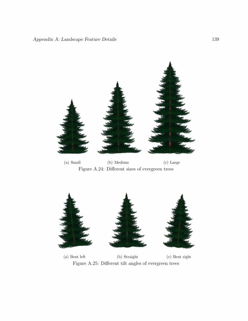
Appendix A: Landscape Feature Details 139
(a) Small (b) Medium (c) Large
Figure A.24: Different sizes of evergreen trees
(a) Bent left (b) Straight (c) Bent right
Figure A.25: Different tilt angles of evergreen trees

140 Automated Landscape Painting in the Style of Bob Ross
Figure A.26: Evergreen trees with downward sloping leaves
Direction of Leaves
There is a variation of evergreen trees where the leaves are sloping downward instead of
upward. See Figure A.26 for a picture of a couple of trees with this property. This option
is implemented by changing a couple of things. Firstly, the rotation of the fan brush that
is used for each stab is subtracted by 180 degrees to flip the leaves upside down. Also,
the stabs on the left side of the tree are painted with the left corner of the fan brush
now, instead of the right, and the stabs on the right side of the tree are painted with the
right corner of the brush. Secondly, the top row of each level now has the most number
of stabs and the amount of stabs in each row decreases for each subsequently lower row.
Thirdly, the highlight rows are painted starting with the lightest paint colour at the top
row of a level and darker highlights are used for each subsequently lower row. Finally, the
last change needed is to limit the number of rows painted in the last level of the tree to
three. This gives the tree a flatter appearance at the bottom, which seems to look more
appropriate. Making these slight modifications to the existing leaf structure and painting
techniques creates a great variation to the evergreen tree feature.

Appendix A: Landscape Feature Details 141
Figure A.27: Evergreen trees at different distances from the viewer
Distance from View
One of the essential adjustable attributes of the evergreen tree feature is the distance
from the viewer. All of the trees in the previous figures have been trees that are close to
the viewer. See Figure A.27 for a picture of three trees, two of which are far away from
the viewer and one that is close. Three simple modifications are made to a close tree to
make it a far tree. The first is to paint the trunk thinner by using stabs with the palette
knife all the way down the tree instead of just at the top. The second modification is to
use a lighter colour scheme to produce the same effect that was used for the Mountain and
Hills features. The final modification is to make the separation between the stabs in every
row a little bit smaller to make trees that are far away slightly thinner than trees that are
close by.
Snow Covered
The evergreen trees can also be adjusted to look like they are in a winter environment
instead of a summer one. See Figure A.28 for a picture of four snow covered trees. The
trees are easily transformed by using a blue colouring scheme instead of a green one. The
highlights now appear as snow on the leaves. The tree with downward sloping leaves looks
better snow covered because it appears that the weight of the snow is pulling the leaves

142 Automated Landscape Painting in the Style of Bob Ross
Figure A.28: Snow covered evergreen trees
down.
Trunk Highlight Side
The last adjustable attribute of the evergreen trees is the highlight side of the trunk.
It is fairly subtle, but the close tree on the right in Figure A.28 has its trunk highlight side
on the left and the close tree on the left has its trunk highlight side on the right. This
is easily switched between trees by changing the side of the trunk that the horizontal line
strokes made with the palette knife start on. Since each layer of highlight colour on the
trunk is painted starting from one side and ending shorter and shorter on the other, the
side that each stroke starts on will be lighter in colour and thus the highlight side of the
trunk.
A.5 Deciduous Tree Feature
Another type of tree that Bob Ross commonly painted in his landscape paintings is a
deciduous tree. There are many different kinds of deciduous trees that he used to paint.
The deciduous trees found in Forest Hills are painted in three stages. First, the trunk of

Appendix A: Landscape Feature Details 143
the tree is painted, then the branches are added to the trunk, and finally, the leaves of the
tree are added to the branches. One of the main differences between the deciduous trees
and the evergreens is that the deciduous trees are not contained within the view of the
scene and seem to grow well above the top of the canvas. Like the evergreen tree feature,
the reference point for the deciduous tree feature is at its bottom, right at the base of its
trunk.
A.5.1 Trunk
The trunk of a deciduous tree is painted using a procedure similar to the one used to
paint the trunk of an evergreen tree. Aside from the obvious difference in size, the only
change in technique is to paint eight layers of colour instead of three. The reasons to
paint more layers of colour for the deciduous tree trunk than for the evergreen tree trunk
is so that the trunk of the deciduous tree will have more detail from paint breaks and a
more gradual change in highlight colour. These two attributes are necessary because the
deciduous tree trunk is larger than an evergreen tree trunk, even at the smallest size. Also,
the deciduous tree trunk is not covered with as many leaves as the trunk of an evergreen
tree, so it is a lot more visible. See Figure A.29 for a picture of a painted deciduous tree
trunk.
To make the trunk of the tree look like it goes well past the top of the canvas, I choose
the top point of a deciduous tree to not be on the canvas, but well above it at a negative
y coordinate value. Nothing happens when the knife, or any brush for that matter, tries
to deposit paint on an area outside the bounds of the canvas. It is important to note that
during a stroke partially off of an edge of the canvas, the PEs of a brush that are on the
canvas can deposit paint while the PEs that are off the canvas cannot. This affordance
allowed by my brush and canvas models allows me to paint the trunk of the deciduous tree,
among other parts of other features, right up to an edge of the canvas with ease.
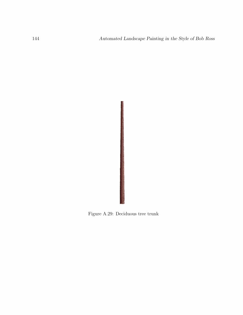
144 Automated Landscape Painting in the Style of Bob Ross
Figure A.29: Deciduous tree trunk

Appendix A: Landscape Feature Details 145
Figure A.30: Deciduous tree branches
A.5.2 Branches
After its trunk is painted, the branches of a deciduous tree are added next. Each indi-
vidual branch is painted using a jagged third degree Bezier curve stroke. See Figure A.30
for a picture of a deciduous with its painted branches.
Sizes
There are three sizes of branches, small, medium, and large. Different sizes of branches
are created by changing the spacing and orientation of their brush stroke control points.
Large branches always have their first control point on the trunk of a tree and tend to
grow outward horizontally, bending upward at the end. Medium sized branches stem off
of large branches and tend to grow mostly upward with a slight bend outward away from

146 Automated Landscape Painting in the Style of Bob Ross
the trunk. Small branches can stem off of the trunk of a tree or off of a medium or large
branch. Small branches have different orientations depending on their location. Small
branches on the trunk grow diagonally upward and away from the trunk according to what
side they are on. Small branches stemming from a large branch grow in the same direction
as if they were stemming from the same side of the trunk, unless they are at the end of
the large branch. In this case, a small branch grows in a slightly more upward direction.
Finally, small branches that stem off of a medium branch have the same shape as if they
were stemming from the trunk, except that each subsequent small branch stemming from
a medium branch alternates in growth direction.
Brush Strokes
Each branch is painted using the filbert brush loaded with a dark brown paint. The
paint amount is enough that it does not run out before the end of the stroke. As the stroke
for each branch progresses, the applied pressure of the brush is reduced so that the end of
each branch will be thinner than its beginning. The starting pressure used for each stroke
depends on the branch size. A light starting pressure is used for small branches, a medium
pressure is used for medium branches, and a high pressure is used for large branches. The
ending pressure used for the brush strokes of all branch sizes is light.
Locations
The starting locations of each branch stemming off of the trunk or other branches are
carefully chosen. Small lone branches are placed randomly along the trunk on alternating
sides. Aside from the lone branches, there are always three large branches that stem from
the trunk, two on one side, one on the other. These branches are generally in the same
locations along the height of the trunk but their exact spacing is randomized.
Each large branch can have either three or four branches stemming from it. The
stemming branches are generally evenly spaced across the large branch but are randomized

Appendix A: Landscape Feature Details 147
within specific thresholds. The last branch stemming from near the end of a large branch
is always a small branch. The first branch is always a medium branch with other small
branches on it. The branches in the middle can be either small or medium at random.
Each medium branch stemming from a large branch can have one to three small
branches stemming from it, chosen at random. The direction of the first small branch
is also chosen at random; however, the directions of subsequent small branches alternate.
Each small branch is generally evenly spaced along a medium branch with some random-
ness. If, for example, a medium branch only has one small branch stemming from it, it will
probably stem from around the middle. Alternatively, if it happens to have two or three
small branches stemming from it, the first small branch will definitely stem from a lower
point on the medium branch and the rest of the small ones will be spaced out along the
rest of the medium branch above the first one.
A.5.3 Leaves
After the branches are complete, the last step to finish painting a deciduous tree is to
add the leaves. See Figure A.31 for a finished deciduous tree. Bob Ross painted the leaves
on the deciduous tree in the same way that he painted his bushes. So the leaves on the
deciduous tree are actually painted as clusters of the bush feature described in Section A.7.
The bushes that are used for the leaves are of size small and flat, they have no branches of
their own, and their highlight side is the same as the highlight side of the deciduous tree.
Each bush can be thought of as a group of leaves on the tree.
Locations
Groups of leaves are painted in three different locations on a deciduous tree. One group
is painted at the end of each large branch. The orientation of these groups is bent left
if the large branch is on the right side of the trunk, bent right otherwise. One group is
painted at the end of each last small branch on each large branch. The orientation of these

148 Automated Landscape Painting in the Style of Bob Ross
Figure A.31: Deciduous tree with leaves
Appendix A: Landscape Feature Details 149
groups of leaves is straight. Finally, a cluster of either two or three groups of leaves, chosen
at random, is painted at the end of each medium branch stemming from a large branch.
If three groups are chosen, they are arranged in a triangle centred around the end of the
branch. Otherwise, the two groups are placed on either side of the end of the branch.
The orientation of these groups is chosen at random from being bent left, bent right, or
straight.
Paint Order
The order that each group of leaves is painted over the branches of a deciduous tree
is important because of the highlights on each group. Each group is highlighted either on
its left or right side and more on the top than the bottom. So, each group has a dark
area and a highlighted area. Painted together in clusters, the groups of leaves look best
when the dark areas covering any highlighted areas are minimized. If all of the dark areas
are painted over all of the highlight areas, none of the highlights will be visible. If some
of the highlights are covered, but others are not, taken together as clusters, the groups of
leaves look strange. The ideal scenario is to have the highlighted areas of newly painted
leaves cover the dark areas of previously painted leaves. If two groups of leaves are painted
side-by-side so that one covers half of the other and the highlights of each group are on the
right, then the group on the right should be painted first, then the group on the left. In
this case, the highlights on the right side of the left group will cover the dark side of the
right group.
To accomplish this paint order for the groups of leaves painted on top of the branches
of a deciduous tree, before any groups are painted, all of their locations are found and
sorted. They are sorted based on what their highlight side is. If their highlight side is on
the left, they are sorted by the distance each of their locations is from the top-left corner
of the canvas. If their highlight side is on the right, they are sorted by the distance each
of their locations is from the top-right corner of the canvas. The groups of leaves whose
locations are the shortest distance from the appropriate corner of the canvas are painted
first. If the highlight side of the tree is on the right, then the groups are painted in a
150 Automated Landscape Painting in the Style of Bob Ross
progression starting from the top-right corner of the tree and moving diagonally down and
to the left toward the bottom-left corner. Painting the groups of leaves in this kind of
order maximizes the amount of highlights visible from each group.
A.5.4 Adjustable Attributes
Size
A deciduous tree can be one of three sizes, small, medium, or large. The width of
the trunk is the main thing that is affected by changing a tree’s size. Since a trunk is
painted with increasingly wider horizontal strokes going from the top of the tree down to
the bottom, adjusting the tree’s height automatically yields an appropriate trunk width.
Aside from a smaller trunk, a small sized tree also has different branches than a medium
or large sized one. Where the large branches would normally stem off of the trunk, medium
branches are stemmed instead. This gives a small sized deciduous tree quite a different
appearance than the medium or large sizes. See Figure A.32 for a picture of two small
sized trees.
Tilt Angle
Figure A.32 also demonstrates how the tilt angle can affect the look of a tree. Orien-
tations other than straight up do not look appropriate for the larger sized trees, but work
well for the small ones. Implementing different tilt angles is simply achieved by adjusting
the location of the top point of a tree relative to its reference point at the bottom.
Side with Two Large Branches
The side of the tree with two large branches instead of one can be toggled between
right and left. Figure A.33 shows a medium sized tree with two large branches on the left

Appendix A: Landscape Feature Details 151
Figure A.32: Two small deciduous trees tilted at different angles

152 Automated Landscape Painting in the Style of Bob Ross
Figure A.33: A deciduous tree with two large branches on the left
of the trunk instead of the right.
Highlight Side
Figure A.33 also shows what a deciduous tree looks like when its highlight side is on the
left instead of the right. Notice that both the trunk and the leaves reflect this attribute.
Leaf Colours
As shown in Figures A.31, A.32, and A.33, the base and highlight colours of the leaves
can be independently changed to any of the colours that the bush feature provides.
Appendix A: Landscape Feature Details 153
A.6 Rocky Bank Feature
Bob Ross painted many kinds of rocks and rocky areas in a lot of his landscape paintings.
In Forest Hills, he painted rocky banks for the trees to sit on. Each rocky bank consists of
several large rocks that have different shapes and sizes. The two inch palette knife is used
to paint the rocks. The one inch and two inch brushes are used dry to paint the reflections
of the rocks. The reference point of the rocky bank feature is at the top-centre of its first
(topmost) rock.
A.6.1 Strokes
Each rock is painted with two sets of strokes. Every stroke within both sets is a jagged
line stroke. The first set of strokes are used to paint the top part of a rock, the second
set of strokes are used to paint the bottom. There are two aspects of the rocky bank that
affect the strokes used to paint it. The first is where the water is with respect to the bank.
This is an adjustable attribute and can be set to either “on the left” or “on the right”.
The other factor that affects a stroke, mainly the top ones, is the slope direction of each
rock. Each rock can have a slope direction of either, up, flat, or down. Every stroke is
pre-calculated and stored so that they can be painted over several times with different
layers of paint.
Top Strokes
The first top stroke always starts at the reference point of the rocky bank feature. The
direction of each stroke depends on where the water is with respect to the rocky bank.
Each top stroke is painted in a direction toward the location of the water. The other factor
that affects the orientation of the top strokes is the slope direction of the rock. If the
slope is up, the top strokes go diagonally upward from their starting point. A flat slope
is painted with strokes that are generally horizontal. Down-sloped rocks are painted with

154 Automated Landscape Painting in the Style of Bob Ross
diagonal strokes that are directed downward. From the reference point, each successive
top stroke starts at a point that is farther away from the water. If the water is on the left
of a rocky bank, each of its top strokes starts to the right of the previous one.
The starting knife rotations used for the top strokes are within random ranges that
depend on the water location and the slope of the rock. The ending knife orientations for
the top strokes are the same for any kind of rock; they are close to being horizontal.
Bottom Strokes
Each top stroke is paired with a bottom stroke. The starting point of each bottom
stroke is the same as the end point of its matching top stroke. Also, the starting knife
rotation of each bottom stroke is the same as the ending rotation of its corresponding
top stroke. The bottom strokes all end on the same horizontal line somewhere below the
bottom of the top strokes. This horizontal line is the water line of the rock. The height
of all of the bottom strokes between the bottom of the top strokes and the water line is
random so that different rocks within a bank will have varied heights above the water. The
ending knife orientation of each bottom stroke is always horizontal so that the rock will
meet the water in a straight and flat line.
A.6.2 Undercoat
Once all of the strokes for a rock are calculated, it can be painted. Each rock within a
rocky bank is painted separately. The first step in painting a rock is to paint its undercoat.
Figure A.34 shows a rocky bank where the first two rocks have been completed and only
the undercoat of the third rock has been painted so far. Every top and bottom stroke
is painted with a dark brown colour of paint. The undercoat paint should not have any
breaks in it, so the 2 inch palette knife is loaded with the maximum paint amount before
each stroke.

Appendix A: Landscape Feature Details 155
Figure A.34: Rock undercoat
Figure A.35: Rock reflection
A.6.3 Reflection
Before any other layers of paint are added to the undercoat of a rock, its reflection is
painted. The reflection is painted before other layers because the bottom texture layer will
get smudged from the reflection strokes if it is painted before them and the top surface
layers must be painted after the bottom texture layer. See Figure A.35 for a picture of the
rock with its reflection.
The reflection is painted using the one and two inch brushes. First, using the two inch
brush dry, vertical strokes starting at the water line of a rock and heading downward are
painted to bring down some of the paint from the undercoat. These strokes span across
the entire water line of the rock and are applied with a high amount of pressure. Then,
three more sets of strokes are used to soften the paint brought down from the undercoat.

156 Automated Landscape Painting in the Style of Bob Ross
Figure A.36: Rock bottom texture
The first set is painted using the 1 inch brush dry and consists of two horizontal strokes
that sweep across the bottom of the rock. One starts from the left side and goes right, the
other vice-versa. These strokes are applied with a high pressure as well. The next set of
strokes are similar to the first set of vertical strokes using the two inch brush dry, except
that a much lighter pressure is used. Finally, the last set of blending strokes is similar to
the second set of horizontal strokes using the 1 inch brush dry, except a light pressure is
used to finish off the reflection.
A.6.4 Bottom Texture
Another layer of paint is added to a rock by painting the same bottom strokes that were
used for the undercoat with a different paint colour and amount. This produces a texture
on the bottom part of a rock that is directly coming out of the water. See Figure A.36 for
a picture of the rock with its bottom texture painted on its undercoat. The paint colour
used is a slightly lighter and more grayish brown than the undercoat colour. The texture is
produced from the breaking pattern of the paint off of the 2 inch palette knife. A medium
amount of paint is loaded on the knife before each bottom stroke to produce the desired
texture.

Appendix A: Landscape Feature Details 157
Figure A.37: Rock top surface
A.6.5 Top Surface
After the bottom texture is painted on a rock using the bottom strokes for a second
time, the top strokes are used again to paint the surface on top of the rock. See Figure A.37
for a picture of the rock after the surface on top of it has been painted. The paint colour
used for the top surface is a lighter, redder, brown than the colour of the undercoat. To
obtain a varied texture for the top surface of a rock, each top stroke is painted twice. The
first time, the whole top stroke is painted. The second time, each top stroke is painted
using two separate strokes, one for the first half and another for the second half. A variety
of random amounts of paint are used for each of these strokes to achieve an assortment of
textures for all of the rocks.
A.6.6 Top Surface Highlights
To vary the texture of the top surface of a rock even more, another layer of paint using
the top strokes is added. See Figure A.38 for a picture of the rock with highlights on its
top surface. The highlights sometimes look like shallow puddles of water on top of the
rock. They are created by painting each top stroke using three separate strokes, one for
each third of the stroke. Each stroke is painted with a small amount of loaded paint.

158 Automated Landscape Painting in the Style of Bob Ross
Figure A.38: Rock top surface highlights
Figure A.39: Rock water ripples
A.6.7 Water Ripples
The last step to finish a rock is to add water ripples along its water line. See Figure A.39
for a picture of the finished rock. Each ripple is painted in the same way as the ripples for
the hills were painted, using a combination of palette knife and one inch brush stabs. The
ripples are painted along the water line of the rock right across the bottom of all of the
bottom strokes. A rocky bank is painted closer to the viewer than the hills are, so some
of the ripples are placed to randomly overlap each other by different amounts, causing a
more varied and thicker appearance of the ripples of a rocky bank than the ripples of the
hills.
A few ripples are also painted out in front of the last rock of the bank, similar to what
Appendix A: Landscape Feature Details 159
was done for the hills. They cannot be seen on the white canvas, however, so I cropped
them out of the figures. They cannot be seen because they are painted well past the
brown reflection of the last rock of the bank. In the Forest Hills landscape however, they
are painted over the relatively dark reflections of the evergreen trees and are much more
visible there.
A.6.8 Rock Layout
The rocks within a rocky bank are placed one after another such that each rock is
placed below and further away from the water than the previous one. So, if the water is
on the left for example, each rock within a bank is placed lower and further to the right
so that the previous rocks are visible. The placement of each rock is of course randomized
so that they are not all located the same distance from each other.
A.6.9 Another Small Rock on Top
If a rock has a flat slope, there is a 50% chance that another smaller rock will be painted
on top of it. The first rock in Figure A.39, for example, has this type of rock. A smaller
rock painted on top of another one is about half the size of the one it is painted on and is
placed slightly to the right of the bottom rock’s horizontal centre. A small rock is painted
in the same way as the normal sized ones except that no water ripples are painted along
its bottom and the ending knife rotations of its bottom strokes are randomized from the
horizontal to make its bottom line a little more jagged.
A.6.10 Adjustable Attributes
There are several attributes that can be adjusted for the rocky bank feature. The
number of rocks in the bank can be between 1 and 5, inclusive. As mentioned before, the
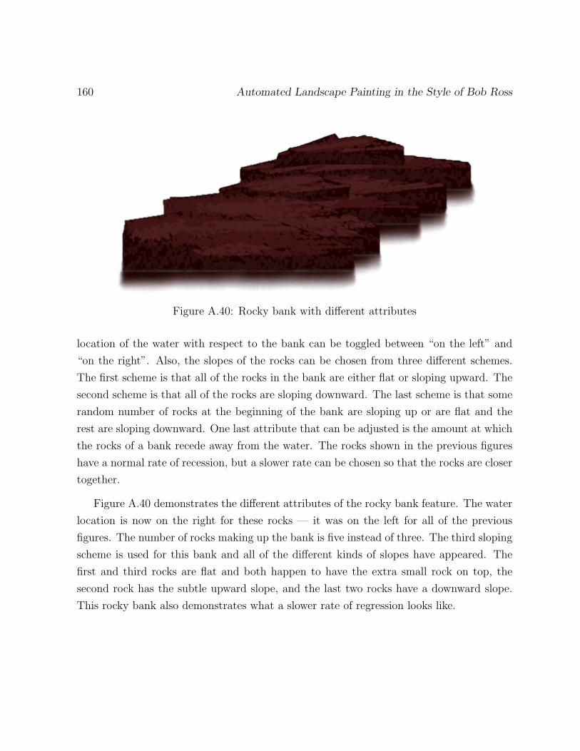
160 Automated Landscape Painting in the Style of Bob Ross
Figure A.40: Rocky bank with different attributes
location of the water with respect to the bank can be toggled between “on the left” and
“on the right”. Also, the slopes of the rocks can be chosen from three different schemes.
The first scheme is that all of the rocks in the bank are either flat or sloping upward. The
second scheme is that all of the rocks are sloping downward. The last scheme is that some
random number of rocks at the beginning of the bank are sloping up or are flat and the
rest are sloping downward. One last attribute that can be adjusted is the amount at which
the rocks of a bank recede away from the water. The rocks shown in the previous figures
have a normal rate of recession, but a slower rate can be chosen so that the rocks are closer
together.
Figure A.40 demonstrates the different attributes of the rocky bank feature. The water
location is now on the right for these rocks — it was on the left for all of the previous
figures. The number of rocks making up the bank is five instead of three. The third sloping
scheme is used for this bank and all of the different kinds of slopes have appeared. The
first and third rocks are flat and both happen to have the extra small rock on top, the
second rock has the subtle upward slope, and the last two rocks have a downward slope.
This rocky bank also demonstrates what a slower rate of regression looks like.

Appendix A: Landscape Feature Details 161
A.7 Bush Feature
The last landscape feature that is painted in Forest Hills is the bush feature. Bushes
are common in Bob Ross’s landscape paintings. He painted them in different shapes, sizes,
and colours, with several variations often appearing in a single landscape. Bob Ross used
the same technique to paint the bushes as he did to paint the leaves on the deciduous tree.
This is why I used one of the variations of the bush feature to paint the leaves for the
deciduous tree feature. Each bush is painted using the one inch brush and a palette knife.
The reference point of the bush feature is at its horizontal centre near its bottom.
A.7.1 Leaf Locations
The leaves of a bush are painted similarly to the leaves of an evergreen tree. All of the
leaf locations are calculated first and then stabs of paint are painted at different subsets
of the locations to create the different layers required.
The leaves of a bush are painted in levels of stabs with the one inch brush. The levels
are painted in succession from the top point of a bush down to its reference point at the
bottom. Each level consists of three stabs, one in the centre of the bush and two on either
side. The brush rotation used for the centre stab of each level is always the same angle
as the tilt angle of the bush. The stabs at the sides of a bush are painted with brush
orientations that start almost vertically and successively approach horizontal angles after
each level. The stabs of a bush are not symmetrical across its vertical axis, the left and
right stabs of each level are painted randomly and independently of each other.
The direction of each leaf stab, that is, which way the bristles of the brush slide during
each stab, are always the same as the brush’s rotation for the stab. This makes each stab
appear like growing leaves that are reaching outward from the centre of the bush.
The separation between each of the stabs in a level increases at each lower level of
a bush. This is to make the bottom of a bush wider than its top. The changing brush

162 Automated Landscape Painting in the Style of Bob Ross
Figure A.41: Bush undercoat
rotation used for each stab already makes a bush wider near the bottom, but it is not
enough on its own for the desired width of the bushes. The leaves near the bottom of a
medium or large sized bush tend to become too sparse because of the separation between
the stabs at the lower levels. To remedy this, a few extra stab locations are added to the
bottom of medium or large sized bushes near their centre stabs to increase the density of
their leaves at these locations.
A.7.2 Undercoat
The first layer of paint that is needed to paint a bush is its undercoat. Each leaf location
is painted with the chosen leaf colour for the bush. See Figure A.41 for a picture of the
undercoat of a large bush with a dark green leaf colour. Each leaf location is painted with
a large stab offset amount, so the bristles of the one inch brush slide on the canvas quite
a bit for each stab.
A.7.3 Branches
After the undercoat of a bush is painted, its branches are scratched in with the corner of
a palette knife. Both sized palette knives have the same effect when used in their alternate
scratching mode, so the size of the knife used to scratch in the branches does not matter.
The number of branches a bush has depends on its size. A small bush, whether it is flat or
not, randomly has either two or three branches, a medium sized bush randomly has four
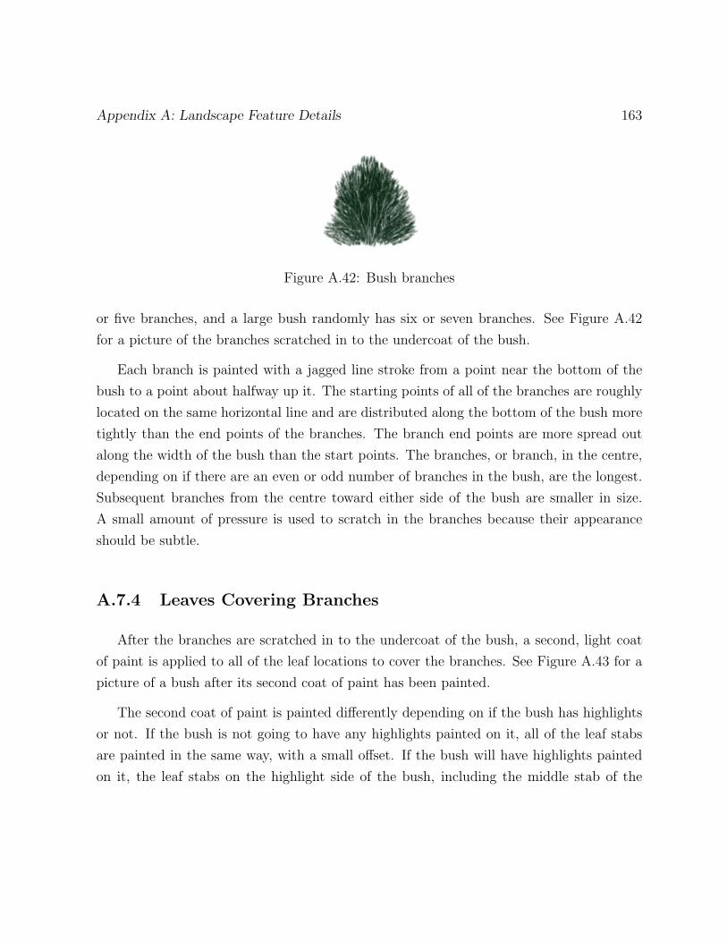
Appendix A: Landscape Feature Details 163
Figure A.42: Bush branches
or five branches, and a large bush randomly has six or seven branches. See Figure A.42
for a picture of the branches scratched in to the undercoat of the bush.
Each branch is painted with a jagged line stroke from a point near the bottom of the
bush to a point about halfway up it. The starting points of all of the branches are roughly
located on the same horizontal line and are distributed along the bottom of the bush more
tightly than the end points of the branches. The branch end points are more spread out
along the width of the bush than the start points. The branches, or branch, in the centre,
depending on if there are an even or odd number of branches in the bush, are the longest.
Subsequent branches from the centre toward either side of the bush are smaller in size.
A small amount of pressure is used to scratch in the branches because their appearance
should be subtle.
A.7.4 Leaves Covering Branches
After the branches are scratched in to the undercoat of the bush, a second, light coat
of paint is applied to all of the leaf locations to cover the branches. See Figure A.43 for a
picture of a bush after its second coat of paint has been painted.
The second coat of paint is painted differently depending on if the bush has highlights
or not. If the bush is not going to have any highlights painted on it, all of the leaf stabs
are painted in the same way, with a small offset. If the bush will have highlights painted
on it, the leaf stabs on the highlight side of the bush, including the middle stab of the

164 Automated Landscape Painting in the Style of Bob Ross
Figure A.43: Bush second coat
Figure A.44: Finished bush with a light green highlight
topmost layer, are painted with a smaller stab offset than the rest of the stabs. The reason
for doing this is that adding highlights to one side of a bush creates an imbalance of paint
on top of the branches, making them look less visible on that side. Having a larger stab
offset on the non-highlight side of the bush during the second coat causes more paint to be
deposited on that side and thus leaves less paint on the highlight side. After the highlights
are painted, both sides of the bush will be roughly balanced with paint and the appearance
of the branches will be uniform across the width of the bush.
A.7.5 Highlights
The last step in painting a bush is to paint its highlights (Figure A.44). All of the
stabs used to paint the highlights are painted with a small stab offset. The highlights are
painted in several layers of stabs. The first layer of stabs includes the locations of all of the
stabs in each level on the highlight side, as well as the middle stab of the level at the top of
the bush. Subsequent layers of highlights are painted at stab locations that are calculated
Appendix A: Landscape Feature Details 165
by moving each of the highlight stab locations from the first layer toward the centre of the
bush. So, if the highlight side of a bush is on its left, each successive layer of highlights is
to the right and slightly below the previous one. To not paint any highlight layers below
the leaves at the bottom of the bush, the bottom-most stab location on the highlight side
is not included in any subsequent highlight layers after the first.
The number of layers of highlights for small, medium, and large sized bushes is 3, 4,
and 5, respectively. The first layer of highlights is painted with the chosen highlight colour
of the bush. The paint colours used for subsequent highlight layers are calculated so that
they gradually approach the leaf colour of the bush. If n is the total number of highlight
layers, i is the current layer number starting at 0 for the first layer, l is the leaf colour,
and h is the original highlight colour, then the equation used to calculate the paint colour
c for a layer of highlight is
c = h +i
n(l − h) (A.1)
Notice from Equation A.1 that the colour used for the first layer of highlights when i = 0
is the original, chosen highlight colour, as mentioned earlier.
A.7.6 Adjustable Attributes
The bush feature has several different adjustable attributes that make it varied and
versatile.
Size
There are four different sizes of bushes available, small and flat, small, medium, and
large. See Figure A.45 for pictures of each size of bush. Different sizes of bushes are mainly
implemented by changing the distance of the top point from the bottom point. Medium
and large sized bushes require extra stabs near their bottom to fill out the leaves. Different
sized bushes also have different numbers of branches that are proportional to their size.
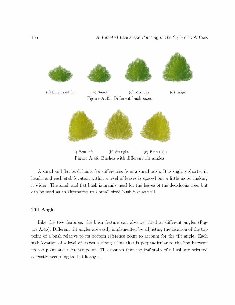
166 Automated Landscape Painting in the Style of Bob Ross
(a) Small and flat (b) Small (c) Medium (d) Large
Figure A.45: Different bush sizes
(a) Bent left (b) Straight (c) Bent right
Figure A.46: Bushes with different tilt angles
A small and flat bush has a few differences from a small bush. It is slightly shorter in
height and each stab location within a level of leaves is spaced out a little more, making
it wider. The small and flat bush is mainly used for the leaves of the deciduous tree, but
can be used as an alternative to a small sized bush just as well.
Tilt Angle
Like the tree features, the bush feature can also be tilted at different angles (Fig-
ure A.46). Different tilt angles are easily implemented by adjusting the location of the top
point of a bush relative to its bottom reference point to account for the tilt angle. Each
stab location of a level of leaves is along a line that is perpendicular to the line between
its top point and reference point. This assures that the leaf stabs of a bush are oriented
correctly according to its tilt angle.

Appendix A: Landscape Feature Details 167
Highlights
A bush can have highlights on either of its sides, or no highlights at all. Aside from
demonstrating different tilt angles, Figure A.46 also shows the different highlighting options
of the bush feature.
Colours
The paint colour used for the leaves and highlights of a bush can be chosen indepen-
dently. A range of four different colours are provided for the leaves and another four for the
highlights. See Figure A.47 for a picture of bushes with all of the different combinations of
colours. The leaf colours are organized in rows and the highlight colours are organized in
columns. The leaf colours used in each row, starting from the top, are dark green, green,
yellowish green, and yellow. The highlight colours used in each column starting from the
left are green, light green, light yellowish green, and light yellow. Notice that there are no
bushes in the lower-left entries of the colour grid. This is because the highlight colour of a
bush should always be lighter than the leaf colour. For example, all of the highlight colours
are lighter than the darkest leaf colour in the first row, but the only highlight colour that
is lighter than the yellow leaf colour in the last row is the light yellow highlight colour.

168 Automated Landscape Painting in the Style of Bob Ross
Figure A.47: Bush colour combinations

Appendix B
Feature Paint Colours
Table B.1: Sky colours
RGB Colour
Sunny Area (255, 255, 170)
Clouds (70, 70, 130)
Table B.2: Mountain colours
RGB Colour
Undercoat (10, 10, 50) +
((60, 60, 60) + (p−m)(30, 30, 30))
Illuminated Snow (255, 255, 255)
Snow Shadows (30, 30, 100) +
((60, 60, 60) + (p−m)(30, 30, 30))−l(10, 10, 10)
p = peakNumber,m = mainPeakNumber, l = ledgeNumber
169
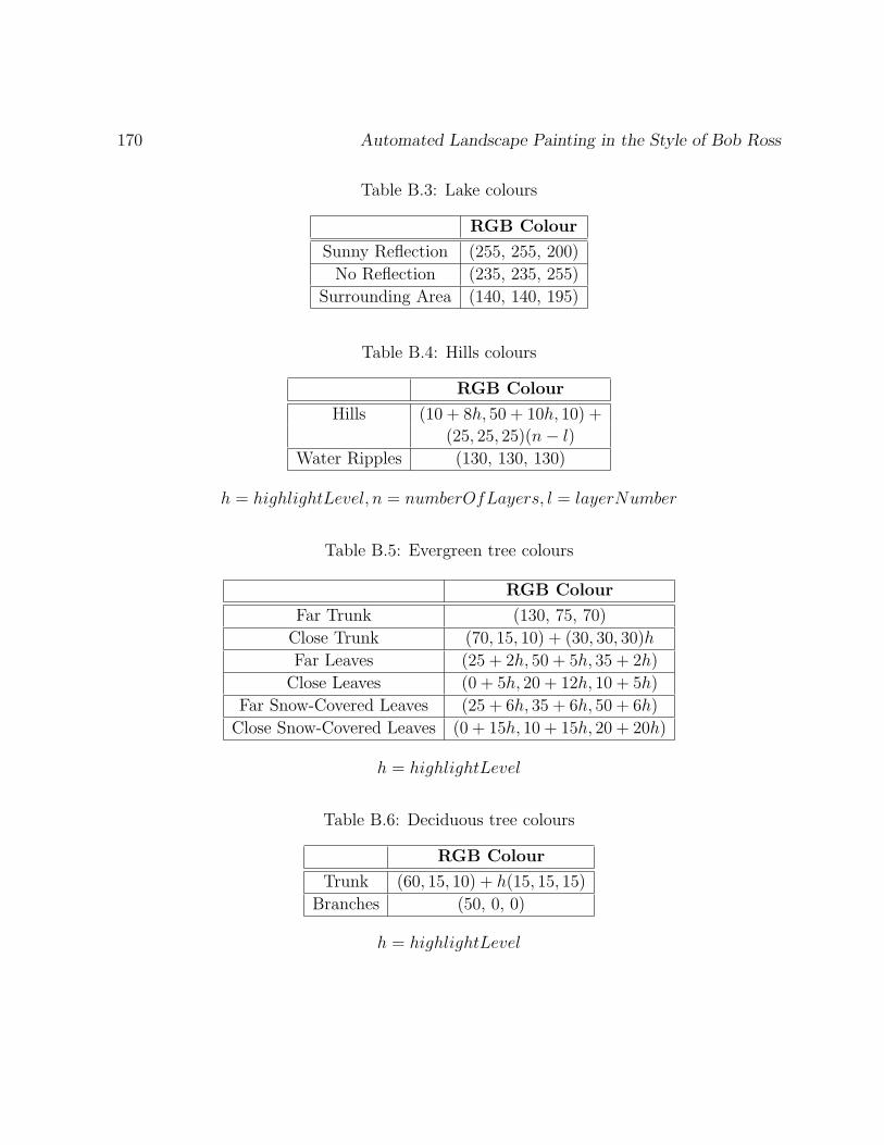
170 Automated Landscape Painting in the Style of Bob Ross
Table B.3: Lake colours
RGB Colour
Sunny Reflection (255, 255, 200)
No Reflection (235, 235, 255)
Surrounding Area (140, 140, 195)
Table B.4: Hills colours
RGB Colour
Hills (10 + 8h, 50 + 10h, 10) +
(25, 25, 25)(n− l)
Water Ripples (130, 130, 130)
h = highlightLevel, n = numberOfLayers, l = layerNumber
Table B.5: Evergreen tree colours
RGB Colour
Far Trunk (130, 75, 70)
Close Trunk (70, 15, 10) + (30, 30, 30)h
Far Leaves (25 + 2h, 50 + 5h, 35 + 2h)
Close Leaves (0 + 5h, 20 + 12h, 10 + 5h)
Far Snow-Covered Leaves (25 + 6h, 35 + 6h, 50 + 6h)
Close Snow-Covered Leaves (0 + 15h, 10 + 15h, 20 + 20h)
h = highlightLevel
Table B.6: Deciduous tree colours
RGB Colour
Trunk (60, 15, 10) + h(15, 15, 15)
Branches (50, 0, 0)
h = highlightLevel

Appendix B: Feature Paint Colours 171
Table B.7: Rocky bank colours
RGB Colour
Undercoat (30, 0, 0)
Top Surface (65, 20, 20)
Top Surface Highlight (75, 30, 30)
Bottom Texture (45, 15, 15)
Water Ripples (80, 80, 80)
Table B.8: Bush colours
RGB Colour
Dark Green Leaves (0, 30, 10)
Green Leaves (0, 60, 10)
Yellowish Green Leaves (50, 100, 10)
Yellow Leaves (140, 140, 0)
Green Highlight (30, 150, 40)
Light Green Highlight (40, 180, 50)
Light Yellowish Green Highlight (170, 220, 20)
Light Yellow Highlight (240, 240, 20)

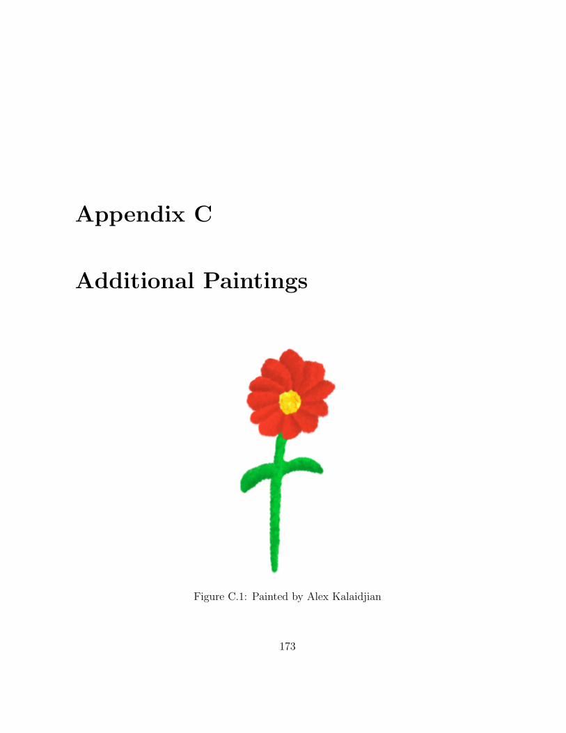
Appendix C
Additional Paintings
Figure C.1: Painted by Alex Kalaidjian
173

174 Automated Landscape Painting in the Style of Bob Ross
Figure C.2: Painted by Jie Xu

Appendix C: Additional Paintings 175
Figure C.3: Painted by Alex Kalaidjian

176 Automated Landscape Painting in the Style of Bob Ross
Figure C.4: Bob Ross’s Winter Evergreens painted by Alex Kalaidjian

Appendix C: Additional Paintings 177
Figure C.5: Bob Ross’s Surf’s Up painted by Alex Kalaidjian

178 Automated Landscape Painting in the Style of Bob Ross
Figure C.6: Forest Hills with a different type of sky

Bibliography
[1] ArtRage 2. [Online; accessed 20-Nov-2006; http://www.ambientdesign.com/
artrage.html].
[2] Corel Painter IX.5. [Online; accessed 20-Nov-2006; http://apps.corel.com/
painterix/home/index.html].
[3] Cassidy J. Curtis, Sean E. Anderson, Joshua E. Seims, Kurt W. Fleischer, and
David H. Salesin. Computer-Generated Watercolor. In SIGGRAPH ’97: Proceed-
ings of the 24th annual conference on Computer graphics and interactive techniques,
pages 421–430, New York, NY, USA, 1997. ACM Press/Addison-Wesley Publishing
Co.
[4] Fast Light Toolkit (FLTK). [Online; accessed 5-Oct-2006; http://www.fltk.org].
[5] A. Gmez de Silva Garza and A. Zamora Lores. Evolutionary Art Revisited: Making
the Process Fully Automated. In Proceedings of the 5th World Scientific and Engi-
neering Academy and Society (WSEAS) International Conference on Soft Computing,
Optimization, Simulation and Manufacturing Systems (SOSM), pages 73–79, 2005.
[6] Paul Haeberli. Paint by Numbers: Abstract Image Representations. In SIGGRAPH
’90: Proceedings of the 17th annual conference on Computer graphics and interactive
techniques, pages 207–214, New York, NY, USA, 1990. ACM Press.
179
180 Automated Landscape Painting in the Style of Bob Ross
[7] James Hays and Irfan Essa. Image and video based painterly animation. In NPAR
’04: Proceedings of the 3rd international symposium on Non-photorealistic animation
and rendering, pages 113–120, New York, NY, USA, 2004. ACM Press.
[8] Aaron Hertzmann. Painterly Rendering with Curved Brush Strokes of Multiple Sizes.
In SIGGRAPH ’98: Proceedings of the 25th annual conference on Computer graphics
and interactive techniques, pages 453–460, New York, NY, USA, 1998. ACM Press.
[9] Aaron Hertzmann. Fast Paint Texture. In NPAR ’02: Proceedings of the 2nd inter-
national symposium on Non-photorealistic animation and rendering, pages 91–ff, New
York, NY, USA, 2002. ACM Press.
[10] William Valentine Baxter III. Physically-Based Modeling Techniques for Interactive
Digital Painting. PhD thesis, University of North Carolina, 2004.
[11] Stephen Mann. A Blossoming Development of Splines. Synthesis Lectures on Com-
puter Graphics, 1(1):1–108, 2006. Morgan-Claypool.
[12] Pamela McCorduck. Aaron’s Code: Meta-Art, Artificial Intelligence, and the Work of
Harold Cohen. Freeman, New York, NY, USA, 1990.
[13] Barbara J. Meier. Painterly Rendering for Animation. In SIGGRAPH ’96: Proceedings
of the 23rd annual conference on Computer graphics and interactive techniques, pages
477–484, New York, NY, USA, 1996. ACM Press.
[14] Bob Ross. The Joy of Painting, volume 9. Bob Ross Publications, 1987.
[15] Steve Strassmann. Hairy Brushes. In SIGGRAPH ’86: Proceedings of the 13th an-
nual conference on Computer graphics and interactive techniques, pages 225–232, New
York, NY, USA, August 1986. ACM Press.
[16] Georges Winkenbach and David H. Salesin. Computer-generated pen-and-ink illus-
tration. In SIGGRAPH ’94: Proceedings of the 21st annual conference on Computer
graphics and interactive techniques, pages 91–100, New York, NY, USA, 1994. ACM
Press.

Bibliography 181
[17] Songhua Xu, Min Tang, Francis Lau, and Yunhe Pan. A Solid Model Based Virtual
Hairy Brush. volume 21, pages 299–308, September 2002.