auto correlation presentation

BS Statistics

6th Semester

Regular

University of Sargodha Session 2011-2015

Introduction Causes of Autocorrelation OLS Estimation BLUE Estimator Consequences of using OLS Detecting Autocorrelation

1. Introduction

Autocorrelation occurs in time-series studies when the errors associated with a given time period carry over into future time periods.

For example, if we are predicting the growth of stock dividends, an overestimate in one year is likely to lead to overestimates in succeeding years.

1. Introduction

Times series data follow a natural ordering over time.

It is likely that such data exhibit intercorrelation, especially if the time interval between successive observations is short, such as weeks or days.

1. Introduction

We expect stock market prices to move or move down for several days in succession.

In situation like this, the assumption of no auto or serial correlation in the error term that underlies the CLRM will be violated.

We experience autocorrelation when

0)( jiuuE

1. Introduction

Sometimes the term autocorrelation is used interchangeably.

However, some authors prefer to distinguish between them.

For example, Tintner defines autocorrelation as ‘lag correlation of a given series within itself, lagged by a number of times units’ whereas serial correlation is the ‘lag correlation between two different series’.

We will use both term simultaneously in this lecture.

1. Introduction

There are different types of serial correlation. With first-order serial correlation, errors in one time period are correlated directly with errors in the ensuing time period.

With positive serial correlation, errors in one time period are positively correlated with errors in the next time period.

2. Causes of Autocorrelation

Inertia - Macroeconomics data experience cycles/business cycles.

Specification Bias- Excluded variable

Appropriate equation:

Estimated equation

Estimating the second equation implies

ttttt uXXXY 4433221

tttt vXXY 33221

ttt uXv 44


Specification Bias- Incorrect Functional Form

tttt vXXY 223221

ttt uXY 221

ttt vXu 223


Cobweb Phenomenon

In agricultural market, the supply reacts to price with a lag of one time period because supply decisions take time to implement. This is known as the cobweb phenomenon.

Thus, at the beginning of this year’s planting of crops, farmers are influenced by the price prevailing last year.


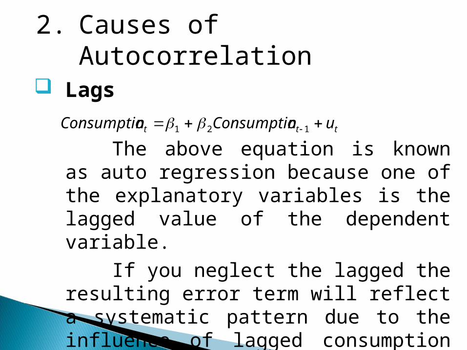
Lags

The above equation is known as auto regression because one of the explanatory variables is the lagged value of the dependent variable.

If you neglect the lagged the resulting error term will reflect a systematic pattern due to the influence of lagged consumption on current consumption.

ttt unConsumptionConsumptio 121


Data Manipulation

This equation is known as the first difference form and dynamic regression model. The previous equation is known as the level form.

Note that the error term in the first equation is not auto correlated but it can be shown that the error term in the first difference form is auto correlated.

ttt uXY 21 11211 ttt uXY

ttt vXY 2


Nonstationarity

When dealing with time series data, we should check whether the given time series is stationary.

A time series is stationary if its characteristics (e.g. mean, variance and covariance) are time variant; that is, they do not change over time.

If that is not the case, we have a non stationary time series.

Suppose Yt is related to X2t and X3t, but we wrongfully do not include X3t in our model.

The effect of X3t will be captured by the disturbances ut. If X3t like many economic series exhibit a trend over time, then X3t depends on X3t-1,X3t -2and so on. Similarly then ut depends on ut-1, ut-2 and so on.

Suppose Yt is related to X2t with a quadratic relationship: Yt=β1+β2X22t+utbut we wrongfully assume and estimate a straight line:Yt=β1+β2X2t+ut

Then the error term obtained from the straight line will depend on X22t.

Suppose a company updates its inventory at a given period in time.

If a systematic error occurred then the cumulative inventory stock will exhibit accumulated measurement errors.

These errors will show up as an auto correlated procedure.

The simplest and most commonly observed is the first-order autocorrelation.Consider the multiple regression model:Yt=β1+β2X2t+β3X3t+β4X4t+…+βkXkt+ut

in which the current observation of the error term ut is a function of the previous (lagged) observation of the error term:ut=ρut-1+et

The coefficient ρis called the first-order autocorrelation coefficient and takes values from -1 to +1.

It is obvious that the size of ρ will determine the strength of serial correlation.

We can have three different cases

If ρ is zero, then we have no autocorrelation. If ρ approaches unity, the value of the previous observation of the error becomes more important in determining the value of the current error and therefore high degree of autocorrelation exists. In this case we have positive autocorrelation. If ρ approaches -1, we have high degree of negative autocorrelation.

Second-order when:ut=ρ1ut-1+ ρ2ut-2+et

Third-order whenut=ρ1ut-1+ ρ2ut-2+ρ3ut-3 +et

p-th order when:ut=ρ1ut-1+ ρ2ut-2+ρ3ut-3 +…+ ρput-p +et

The OLS estimators are still unbiased and consistent. This is because both unbiasedness and consistency do not depend on assumption 6 which is in this case violated.

The OLS estimators will be inefficient and therefore no longer BLUE.

The estimated variances of the regression coefficients will be biased and inconsistent, and therefore hypothesis testing is no longer valid. In most of the cases, the R2 will be overestimated and the t-statistics will tend to be higher.

There are two ways in general.The first is the informal way which is

done through graphs and therefore we call it the graphical method.

The second is through formal tests for autocorrelation, like the following ones:

The Durbin Watson TestThe Breusch-Godfrey TestRun test

The following assumptions should be satisfied:

The regression model includes a constantAutocorrelation is assumed to be of first-

order onlyThe equation does not include a lagged

dependent variable as an explanatory variable

Step 1: Estimate the model by OLS and obtain the residuals

Step 2: Calculate the DW statistic Step 3: Construct the table with the

calculated DW statistic and the dU, dL, 4-dU and 4-dL critical values.

Step 4: Conclude

It is a Lagrange Multiplier Test that resolves the drawbacks of the DW test.

Consider the model:Yt=β1+β2X2t+β3X3t+β4X4t+…+βkXkt+ut

where:ut=ρ1ut-1+ ρ2ut-2+ρ3ut-3 +…+ ρput-p +et

Combining those two we get:Yt=β1+β2X2t+β3X3t+β4X4t+…+βkXkt+

+ρ1ut-1+ ρ2ut-2+ρ3ut-3 +…+ ρput-p +et

Topic Nine Topic Nine Serial Correlation Serial Correlation

The null and the alternative hypotheses are:

H0:ρ1= ρ2=…= ρp=0 no autocorrelation Ha:at least one of the ρ’s is not zero, thus, autocorrelation

Step 1: Estimate the model and obtain the residualsStep 2: Run the full LM model with the number of lags used being determined by the assumed order of autocorrelation.Step 3: Compute the LM statistic = (n-ρ)R2from the LM model and compare it with the chi-square critical value.Step 4: Conclude


We have two different cases:When ρ is knownWhen ρ is unknown

Consider the modelYt=β1+β2X2t+β3X3t+β4X4t+…+βkXkt+ut

whereut=ρ1ut-1+et


Write the model of t-1:Yt-1=β1+β2X2t-1+β3X3t-1+β4X4t-1+…+βkXkt-1+ut-1

Multiply both sides by ρto getρYt-1= ρβ1+ ρβ2X2t-1+ ρβ3X3t-1+ ρβ4X4t-1

+…+ ρβkXkt-1+ ρut-1

Subtract those two equations:Yt-ρYt-1= (1-ρ)β1+ β2(X2t-ρX2t-1)+ β3(X3t-ρX3t-1)+

+…+ βk(Xkt-ρXkt-1)+(ut-ρut-1)

orY*t= β*1+ β*2X*2t+ β*3X*3t+…+ β*kX*kt+et


Where now the problem of autocorrelation is resolved because et is no longer autocorrelated.

Note that because from the transformation we lose one observation, in order to avoid that loss we generate Y1 and Xi1 as follows:Y*1=Y1 sqrt(1- ρ2)

X*i1=Xi1 sqrt(1-ρ2)

This transformation is known as the quasi-differencing or generalised differencing.

The Cochrane-Orcutt iterative procedure.Step 1: Estimate the regression and obtain residualsStep 2: Estimate ρ from regressing the residuals to its lagged terms.Step 3: Transform the original variables as starred variables using the obtained from step 2.

Step 4: Run the regression again with the transformed variables and obtain residuals.

Step 5 and on: Continue repeating steps 2 to 4 for several rounds until (stopping rule) the estimates of from two successive iterations differ by no more than some preselected small value, such as 0.001.

MUHAMMAD IRFAN HUSSIAN(39)

DR ANWAR UL HAQ ( 28)

AMMER UMER (MPA) (30)

CH AAMAR LASHARI (45)

Thank Thank YouYou

Thank Thank YouYou

auto correlation presentation

Education