author's personal copy - universität passau€¦ · article info abstract ......

This article appeared in a journal published by Elsevier. The attachedcopy is furnished to the author for internal non-commercial researchand education use, including for instruction at the authors institution

and sharing with colleagues.

Other uses, including reproduction and distribution, or selling orlicensing copies, or posting to personal, institutional or third party

websites are prohibited.

In most cases authors are permitted to post their version of thearticle (e.g. in Word or Tex form) to their personal website orinstitutional repository. Authors requiring further information

regarding Elsevier’s archiving and manuscript policies areencouraged to visit:

http://www.elsevier.com/copyright

http://www.elsevier.com/copyright

Author's personal copy

Equities, credits and volatilities: A multivariate analysis of the European marketduring the subprime crisis

Irene Schreiber a, Gernot Müller a, Claudia Klüppelberg b, Niklas Wagner c,⁎a Center for Mathematical Sciences, Technische Universität München, Boltzmannstrasse 3, 85748 Garching, Germanyb Center for Mathematical Sciences, and Institute for Advanced Study, Technische Universität München, Boltzmannstrasse 3, 85748 Garching, Germanyc Department of Business and Economics, University of Passau, Innstrasse 27, 94030 Passau, Germany

a b s t r a c ta r t i c l e i n f o

Article history:Received 3 July 2012Accepted 7 July 2012Available online 17 July 2012

JEL classifications:G01C32

Keywords:Credit riskCredit default swapsiTraxx indexVector autoregressionMultivariate GARCHBEKK

We study the lead–lag dependence between aggregate credit spreads and equity prices as well as implied equityvolatility, which is important for proper credit risk assessment. Our analysis includes daily quotes of the iTraxxEurope index, the Dow Jones Euro Stoxx 50 index, and the Dow Jones VStoxx index during the period of June2004 to April 2009, i.e. before and during the subprime financial crisis. We robustly estimate a vectorautoregressive (VAR) model, allow for time-varying coefficients and assume a multivariate autoregressive con-ditional heteroskedastic (ARCH) model of the BEKK-type for the innovations. We find that while the commonlypredicted negative relation between asset prices and credit spreads holds during the pre-crisis period, it fails tohold during the subsequent crisis period. Equity returns turn out to be insignificant predictors of spreads duringthe crisis and spread changes significantly and positively lead changes in equity market volatility. Hence, whileinformation in aggregate spreads is typically not driving aggregate market risk, it well may do so during a periodin which severe stress in credit markets spills over to the equity market. In sum our results cast some doubt onthe stability of the predictions of structural models of credit risk during periods of market stress.

© 2012 Elsevier Inc. All rights reserved.

1. Introduction

The driving factors behind credit risk are of importance in manyareas of applied financial economics. Several authors have empiricallystudied the relationship between credit derivatives, namely creditdefault swap (CDS) spreads, and key spread determinants as predictedby structural models of credit risk (see for example Houweling andVorst (2005), Byström (2005, 2006), Alexander and Kaeck (2006),Sougné, Heuchenne, and Hübner (2008), Ericsson, Jacobs, and Oviedo(2009) andNorden andWeber (2009)). However, recent developmentsin light of the U.S. subprime and the subsequent global financial crisishave shown that credit derivatives – which are at the core of the crisis– exhibit a much more complex dependence relation with explanatoryfinancial variables than previously assumed.

In the present paper we study the lead–lag dependence betweenaggregate credit spreads and equity prices as well as equity volatilityin more detail. Structural models of credit risk predict a negative re-lation between price and spread levels as well as a positive relationbetween volatility and spread levels. While most of the empiricalstudies so far concentrate on modeling the conditional mean (e.g. byfitting regression type models), our modeling approach goes one stepfurther by including the time-varying conditional covariance structure.

We particularly investigate the dependence structure between aggre-gate index credit spreads on the one hand and equity returns andchanges in implied equity volatility on the other. We do this for theEuropean market based on the iTraxx Europe, the Euro Stoxx 50 andthe VStoxx index. We account for the effects of the subprime crisisusing daily quotes during the period of June 2004 to April 2009. Weestimate a vector autoregressive (VAR)model for the lead–lag relations.We extend the standard VAR approach by admitting time-varying coef-ficients and perform robust iteratively re-weighted least squares esti-mation (see Huber, 1981). We thereby reduce the influence of outliersand enhance model adequacy. Following Engle and Kroner (1995) as aspecial case of Bollerslev, Engle, and Wooldridge (1988), we assume amultivariate autoregressive conditional heteroskedastic (ARCH) modelof the BEKK-type for the innovations. The BEKK parametrization guaran-tees the positive definiteness of the conditional covariance matrix andthe number of parameters is remarkably reduced. Most of the depen-dence structure is captured by our VAR-BEKK(2,2)model. Themodel re-siduals are white noise, yet they are not normally distributed.

We find that the inverse relation between the asset price factorand credit spreads indeed significantly holds during the pre-crisisperiod, while it fails to hold during the subsequent crisis period.Hence, our results cast some doubt on the stability of the predictionsof structural models of aggregate credit risk during periods of marketstress. In fact, equity returns turn out to be insignificant predictors ofspreads during the crisis. Our estimation results reveal a further

International Review of Financial Analysis 24 (2012) 57–65

⁎ Corresponding author. Tel.: +49 851 509 3241; fax: +49 851 509 3242.E-mail address: [email protected] (N. Wagner).

1057-5219/$ – see front matter © 2012 Elsevier Inc. All rights reserved.doi:10.1016/j.irfa.2012.07.006

Contents lists available at SciVerse ScienceDirect

International Review of Financial Analysis


interesting characteristic in the predictability of market risk, whichis novel to the literature. While spreads typically lag equity markets,we find that this is not the case during the subprime crisis period. Incontrast, we find that spread changes significantly and positivelylead changes in equity market volatility. Hence, while informationin aggregate spreads is typically not driving aggregate market risk,it may well do so during a period in which severe stress in creditmarkets spills over to the equity market.

In terms of the conditionalmean, our results extend previous empir-ical studies, allowing for robustly estimated, time-varying coefficients.However, to the best of our knowledge, there are no existing studiesof aggregate index credit spreads, stocks and stock market volatility inwhich the conditional covariance structure is considered. We provideevidence of strongly varying conditional variances and correlations,with the dependencies increasing after the outbreak of the financialcrisis.

The remainder of this paper is organized as follows. In Section 1 webriefly introduce themodeling framework. Section 2 is dedicated to ourempirical study of the aggregate credit spread changes. Section 3concludes.

2. Model specification and estimation

2.1. Model

In this section we briefly introduce the necessary theory which wewill apply to our data in Section 2. All stochastic objects in this paperare defined on the probability space Ω;F; Pð Þ. Consider a vector stochas-tic process (yt)t∈Z, i.e. yt : Ω→RN . As usual, we condition on the sigmafield, denoted by Ft−1, generated by the past information until timet-1. Note that we will follow the convention of using lowercase lettersto denote either a random variable or its realization as a time series.In this paper we will consider the following vector autoregressivegeneralized conditional heteroskedastic (VAR-GARCH) model:

yt ¼ cþΦ1yt−1 þ ⋯þΦpyt−p þ εt ; ð1Þ

εt ¼ H1=2t θð Þzt ; zt∼WN 0; INð Þi:i:d:; ð2Þ

where c∈RN denotes a vector of constants,Φ1;…;Φp∈RN�N are matri-ces of autoregressive coefficients and θ∈Θ contains all GARCH parame-ters. Furthermore, ztð Þt∈Z is amultivariatewhite noise process, IN∈RN�N

as usual is the identity matrix and H1=2t θð Þ∈RN�N is a positive definite

matrix, such that Ht is the conditional covariance matrix of yt, e.g. Ht1/2

may be obtained by the Cholesky factorization of Ht.The conditional mean part of the model in Eq. (1) is given by a VAR

model of order p, while the conditional covariancematrixHt in Eq. (2) isspecified by an MGARCH model. As mentioned above, in this work wefocus on one of the most prominent MGARCH models, the BEKKmodel by Engle and Kroner (1995), whichwill be briefly discussed here.

Assume (yt),(εt) and (zt) to be vector stochastic processes as givenby Eqs. (1) and (2). The BEKK(p,q)1 model by Engle and Kroner(1995) for the conditional covariance matrix Ht∈RN�N is defined as

Ht ¼ C′C þXqi¼1

A′iεt−iε

′t−iAi þ

Xpj¼1

B′jHt−jBj; ð3Þ

whereAi;Bj;∈RN�N are parametermatrices andC∈RN�N is an upper tri-angular matrix. As mentioned above the main advantage of this modelis, that the BEKK parametrization automatically guarantees the positive

definiteness of Ht. The number of parameters in the BEKK model isN(N+1)/2+N2(p+q), i.e. O(N2). In order to reduce the number of pa-rameters, different simplifications of the model evolved, e. g. the diago-nal BEKK model where Ai and Bj in Eq. (3) are diagonal matrices or thescalar BEKK model where Ai and Bj are each replaced by a scalartimes a matrix of ones. To ensure the uniqueness of the parame-trization, certain restrictions have to be imposed on the coefficientmatrices. For instance, in the special case of the BEKK(1,1) modelwith Ht=C′C+A′εt−1ε′t−1A+B′Ht−1B and parameter matricesA=(Aij)i,j=1

N ,B=(Bij)i,j=1N Engle and Kroner (1995) show, that

uniqueness is achieved by requesting all diagonal elements of C tobe positive, as well as A11,B11>0. These conditions for the coeffi-cient matrices can be extended to the general case when p,q>1.Engle and Kroner (1995) also show, that the BEKK model as definedin Eqs. (1), (2) and (3) is stationary if and only if all eigenvalues of thematrix ∑ i=1

q A′i⊗Ai+∑ j=1p B′j⊗Bj are less than one in modulus.

2.2. Estimation

Regarding the estimation of the model parameters in Eqs. (1), (2)and (3) we follow a two step approach, where in the first step the pa-rameters of the VARmodel, and in the second step the GARCH parame-ters are estimated.

Concerning the VAR model coefficients we pursue the robust itera-tively re-weighted least squares (RLS) approach of Huber (1981). As-sume that the sample size is T and that we are given p pre-samplevalues y−p+1,…,y0. We define:

Y ¼ y1;…; yTð Þ∈RN�T;

Π ¼ c;Φ1;…;Φp

� �∈RN� Npþ1ð Þ

; π ¼ vec Πð Þ∈RN Npþ1ð Þ;

xt ¼ ð1; y′t−1;…; y′t−pÞ′∈RNpþ1; X ¼ x1;…; xTð Þ∈R Npþ1ð Þ�T

;

E ¼ ε1;…; εTð Þ∈RN�T;

where vec(⋅) is the column stacking operator that stacks the columns ofam×nmatrix as a vector of dimensionmn. Using this notation wemaythen rewrite Eq. (1) as a linear model

Y ¼ ΠX þ E; or equivalently vec Yð Þ ¼ X′⊗IN� �

π þ vec Eð Þ; ð4Þ

where⊗ denotes the Kronecker product or direct product of twomatri-ces. Note that as opposed to classical linear modeling, the matrix ofcovariables contains lagged dependent variables.

The unknown parameters of the VARmodel contained in π in Eq. (4)are then estimated by the RLS approach of Huber (1981), who intro-duces the class of M-estimates, in order to reduce the influence of out-liers and achieve distributional robustness. We investigate the problem∑ i=1

NT ρ(xi;π)=min!, or equivalently ∑ i=1NT ψ(xi;π)=∑ i=1

NT wixi=0,where xi is the i-th residual of the NT-dimensional linear model in Eq.(4), ρ(x;π) is a weighting function, ψ(x)=(∂/∂θ)ρ(x;π) and wi=ψ(xi;π)/xiw. The weighting function ρ(x;π) is assumed to be twice con-tinuously differentiable in x almost everywhere, with nonnegative sec-ond derivative wherever defined. Huber (1981) proposes

ρ xð Þ ¼ x2=2 : jxj≤c;cjxj−c2=2 : jxj > c;

(ð5Þ

which implies weightswi=1 if |xi|≤c andwi=c/xi if |xi|>c. In the con-text of VARmodels strong consistency of the RLS estimator is e.g. shownby Campbell (1982), while asymptotic normality is derived by Li andHui (1989).

1 The acronym BEKK stands for Baba, Engle, Kraft & Kroner who wrote an earlier ver-sion of the paper by Engle & Kroner (1995) (see Engle, Kroner, Baba, & Kraft, 1993).

58 I. Schreiber et al. / International Review of Financial Analysis 24 (2012) 57–65


For the BEKK model given by Eqs. (2) and (3) we perform maxi-mum likelihood (ML) estimation. Assume we have a given samplesize of t=1,…,T. The log likelihood function is then given by

L θð Þ ¼ −12

XTt¼1

Nln 2πð Þ þ ln Ht θð Þj j þ ε′tHt θð Þ−1εt� �

; ð6Þ

where θ ¼ vec C;A1;…;Aq;B1;…;Bp

� �∈Θ⊂RN Nþ1ð Þ=2þN2 pþqð Þ contains

all unknown GARCH parameters. The likelihood function is maxi-mized with respect to θ by using numerical methods. A closed formsolution does not necessarily exist, due to the nonlinearity of the like-lihood function. For asymptotic properties of the ML estimator, seee.g. Comte and Lieberman (2003), who derive strong consistencyand asymptotic normality.

3. Empirical analysis

3.1. Data set

Our data set consists of three time series, the Dow Jones Euro Stoxx50 index, the Dow Jones VStoxx index, a volatility index based on op-tions on the Euro Stoxx 50 and the CDS index iTraxx Europe. In our anal-ysis we focus on the iTraxx Europe benchmark index with a maturity offive years, as this is the most liquid index within the iTraxx Europeindex family. As the membership of the iTraxx is adjusted every sixmonths by issuing a new index series, we construct a time series thatcontains the most recent series at any point in time. In this way we en-sure that our analysis is always built on themost liquid names. The dataperiod starts on June 23, 2004 and ends on April 30, 2009, i.e. the dataset covers 1230 daily quotes for each of the time series. Basic character-istics of the data are summarized in Table 1. The data was transformed

to

Table 1Basic characteristics of the data set. Left: whole period, middle: first “tranquil” period, right: last “volatile” period.

2004-06-23 to 2009-04-30 2004-06-23 to 2007-08-15 2007-08-16 to 2009-04-30

itraxx eurost. vstoxx itraxx eurost. vstoxx itraxx eurost. vstoxx

Min. 20.09 1809.98 11.60 20.09 2580.04 11.60 29.10 1809.98 17.241st qu. 31.00 2980.13 14.85 27.78 3055.85 14.03 68.28 2451.58 22.56Median 37.12 3524.58 17.72 35.20 3544.58 15.67 101.38 3429.58 27.32Mean 59.72 3463.51 22.13 33.38 3537.33 16.15 108.71 3326.18 33.263rd qu. 74.37 3987.13 24.00 37.19 3988.04 17.58 154.42 3881.09 42.05Max. 215.92 4557.57 87.51 68.20 4557.57 30.74 215.92 4489.79 87.51std. 46.43 654.60 11.85 7.41 540.75 2.96 48.71 808.63 13.97Skewn. 1.57 −0.31 2.20 0.42 0.10 1.34 0.21 −0.24 1.18Kurt. 4.26 2.28 8.03 3.65 1.88 5.52 1.89 1.70 3.82

5010

015

020

0

itrax

x (b

ps)

−20

020

−20

020

−20

020

log.

diff

. itr

axx

2000

3000

4000

euro

stox

x

log.

diff

. eur

osto

xx

2040

6080

vsto

xx (

%)

01/05 01/06 01/07 01/08 01/0901/05 01/06 01/07 01/08 01/09

01/05 01/06 01/07 01/08 01/0901/05 01/06 01/07 01/08 01/09

01/05 01/06 01/07 01/08 01/0901/05 01/06 01/07 01/08 01/09

log.

diff

. vst

oxx

Fig. 1. Daily quotes of the iTraxx Europe, the Euro Stoxx 50 and the VStoxx index between 2004-06-23 and 2009-04-30.

59I. Schreiber et al. / International Review of Financial Analysis 24 (2012) 57–65


logarithmic differencesmultiplied by onehundred (see Fig. 1). Evidenceof simple trends and seasonality was not found. Note, that on thewholeiTraxx and Euro Stoxx show counter trends, whereas iTraxx and VStoxxindicate a positive interrelation. The three time series display typicalstylized features such as volatility clustering and at least one structuralbreak, which e.g. inmid 2007 is related to the rise of the subprime crisis.The characteristics of the time series, e.g. in terms ofmean and volatilitylevels, change significantly before and after the outbreak of the crisis(see Table 1), thereby the biggest structural changes are visible in theiTraxx index. The estimated corresponding autocorrelation functionsof the data and the squared data, as well as the corresponding cross cor-relations between the time series can be found in Fig. 2. We see someautocorrelation in the time series, especially within the iTraxx at lagone, however the values are rather small. Cross correlations are perceiv-able only at lag zero. The autocorrelations and cross correlations in thesquared data give rise to the hypothesis of stochastic volatility.

3.2. A VAR model for the conditional mean

In a first step, in order to capture the weak autocorrelation in thedata as seen in Fig. 2, we model the conditional mean of the time seriesby fitting a VARmodel as given by Eq. (1) to the data, i.e. y1,t representsthe iTraxx, y2,t the Euro Stoxx and y3,t the VStoxx index. In order to de-termine the model order p, we fit different models up to order p=10

via ML estimation and calculate the associated information criteriaAIC, HQ and SC (see Akaike, 1973, 1974; Hannan & Quinn, 1979 andSchwarz, 1978). As displayed in Table 2, AIC suggests p=4, whereasHQ and SC both recommend model order p=1. We therefore fit aVAR(1)model to our data.When conductingML estimation of the coef-ficientmatrixΦwefind that six out of nine coefficients are insignificant.Precisely only the coefficients Φ11, Φ21 and Φ33 are significant at a 90%confidence level. We also observe that the coefficient matrix containsmostly very small values. In order to gain deeper insight into the vectorautoregressive structure of our data set we therefore conduct a rollingwindow analysis of the coefficient matrix. We use different windowsfrom 25 to 300 days, finding that all coefficients vary over time, somevery strongly and even changing their signs. This explains the largenumber of insignificant close to zero coefficients which we observedin thefirst place. Additionallywe observe that the coefficients react sen-sitively to apparent outliers in the original data. For this reason we

0 5 10 15 20 25 30

00.

40.

8A

CF

itra

xx

0 5 10 15 20 25 30

00.

40.

8A

CF

eur

osto

xx

0 5 10 15 20 25 30

00.

40.

8

AC

F v

stox

x

0 5 10 15 20 25 30

00.

40.

8A

CF

itra

xx^2

0 5 10 15 20 25 30

00.

40.

8A

CF

eur

osto

xx^2

0 5 10 15 20 25 30

00.

40.

8

AC

F v

stox

x^2

−20 10 0 10 20

−0.

50

0.5

CC

F it

raxx

, eur

osto

xx

−20 10 0 10 20

−0.

50

0.5

CC

F it

raxx

, vst

oxx

−20 10 0 10 20

−0.

50

0.5

CC

F e

uros

toxx

, vst

oxx

−20 10 0 10 20

00.

20.

4

CC

F it

raxx

^2, e

uros

toxx

^2

−20 10 0 10 20

00.

20.

4

CC

F it

raxx

^2, v

stox

x^2

−20 10 0 10 20

00.

20.

4C

CF

eur

osto

xx^2

, vst

oxx^

2

Fig. 2. Autocorrelations and cross correlations of the data set with 95% confidence bounds.

Table 2Order selection criteria AIC, HQ and SC for our data set.

p 1 2 3 4 5 6 7 8 9 10

AIC(p) 5.735 5.737 5.735 5.723 5.730 5.731 5.736 5.736 5.741 5.746HQ(p) 5.754 5.770 5.782 5.784 5.806 5.821 5.840 5.854 5.873 5.893SC(p) 5.785 5.825 5.860 5.886 5.931 5.970 6.012 6.050 6.092 6.135



decide in favor of the RLS estimation procedure by Huber (1981), withthe Huber weighting function as defined in Eq. (5).

We again conduct a rolling window analysis, this time estimat-ing robustly (see Fig. 3). In comparison with the ML estimates, theinfluence of outliers is remarkably reduced, however we findthat both with ML and RLS estimation, the coefficients are time-varying and often change their signs. Consequently we will followa robustly estimated VAR(1) approach with a time-varying coeffi-cient matrix.

In the following we assess the question of which entries of the coeffi-cientmatrix in Fig. 3may be set to zero and, as a consequence, will not beincluded in the further analysis. For this purpose, we simultaneously fol-low two criteria. For the first criterion we split the time series intotwo disjoint parts, namely the first 800 data points (2004-06-23 to2007-08-15) and the last 430 data points (2007-08-16 to 2009-04-30).This partition splits our time series into a “tranquil” period precedingthe subprime crisis, and a “volatile”period startingmid of 2007. Separate-ly analyzing these twoperiods is self-evident given the apparent structur-al breaks in the original data (see Fig. 1) and the coefficient matrixstructure (see Fig. 3). We then perform RLS estimation for each periodseparately. The results are displayed in Table 3. For the tranquil period,

Φ11 andΦ12 are significant, whereas for the volatile period,Φ11 andΦ31

are significant on a 90% confidence level. As a first criterion for whichcoefficients to include in the analysis we follow the convention of ad-mitting all coefficients that are significant on a 90% level at least inone of the two periods. According to this criterion Φ11, Φ12, Φ31, andΦ33 are included in our analysis. However, this criterion has the draw-back that it excludes coefficients that are strongly time-varying andthus may only be significant for certain short time periods. As a secondcriterion for which coefficients to admit for the analysis we thereforedecide to admit strongly time-varying coefficients, in addition to thosebeing significant according to the first criterion. This means that addi-tionally Φ32 is included as well. Therefore, as a final model regardingthe conditional mean, we propose a VAR(1) modeling approach withrobustly estimated, time-varying coefficients and with Φ13=Φ21=Φ22=Φ23 set to zero. Due to the fact that we set some coefficients tozero, the five non-zero entries in the coefficientmatrix have slightly dif-ferent values from those displayed in Fig. 3, yet the overall structure ofthe coefficients remains unchanged.

The estimation results indicate persistent iTraxx spread changes interms ofϕ11 during the overall sample period. Thisfinding can be attrib-uted to the relatively low liquidity of the market for credit risk. In

200 600 1000

200 600 1000

200 600 1000

200 600 1000

200 600 1000

200 600 1000

200 600 1000

200 600 1000

200 600 1000

−4

−2

02

4Φ

11

Φ12

Φ13

−4

−2

02

4Φ

21

Φ22

Φ23

−4

−2

02

4

−4

−2

02

4−

4−

20

24

−4

−2

02

4

−4

−2

02

4−

4−

20

24

−4

−2

02

4

Φ31

Φ32

Φ33

Fig. 3. Robust weighted LS estimation of Φ, using 100 day rolling windows. 95% confidence bounds.

Table 3RLS estimation of the coefficients of the VAR(1) model for different time periods. Left: whole period, middle: “tranquil” period, right: “volatile” period.

Weighted LS estimation

(2004-06-23 to 2009-04-30) (2004-06-23 to 2007-08-15) (2007-08-16 to 2009-04-30)

est. std.error t-stat. est. std.error t-stat. est. std.error t-stat.

c1 0.077 0.112 0.688 0.041 0.151 0.272 0.165 0.092 1.793c2 −0.015 0.042 −0.357 0.055 0.041 1.341 −0.126 0.093 −1.355c3 0.052 0.151 0.344 0.034 0.161 0.211 0.022 0.199 0.111Φ11 0.190 0.022 8.832 0.141 0.019 7.495 0.309 0.058 5.303Φ12 −0.032 0.073 −0.435 −0.390 0.104 −3.755 0.064 0.169 0.380Φ13 0.021 0.019 1.109 0.001 0.018 0.038 −0.063 0.055 −1.143Φ21 −0.002 0.009 −0.208 0.014 0.010 1.362 −0.033 0.021 −1.566Φ22 −0.010 0.031 −0.324 −0.078 0.056 −1.404 −0.002 0.061 −0.027Φ23 0.006 0.008 0.767 −0.010 0.010 −1.096 0.030 0.020 1.501Φ31 0.084 0.044 1.899 −0.069 0.059 −1.175 0.194 0.072 2.689Φ32 0.008 0.151 0.053 0.461 0.324 1.421 0.045 0.209 0.217Φ33 −0.074 0.039 −1.924 −0.020 0.055 −0.359 −0.076 0.068 −1.109



contrast to themarket for credit risk, if we look atϕ22 the equitymarketis characterized by uncorrelated changes in our sample, a finding thatindicates thatmicrostructure induced linear time-series dependence ef-fects in Stoxx index returns are weak. The results for ϕ33 also show that

Table 4AIC criterion for the model order selection in the BEKK model.

BEKK(1,1) BEKK(1,2) BEKK(2,1) BEKK(2,2)

AIC 6221.836 6189.417 6192.885 6187.527

Table 5Coefficients and eigenvalues of the reduced BEKK(2,2) model (2004-06-23 to 2009-04-30). 28/28 significant parameters.

est. std.error t-stat.

C 0.358 0.000 0.816 0.076 0.000 0.236 4.692 – 3.4560.000 0.252 −2.376 0.000 0.071 0.419 – 3.523 −5.6710.000 0.000 0.232 0.000 0.000 0.111 – – 2.090

A1 0.678 −0.033 0.215 0.043 0.011 0.061 15.741 −3.007 3.5210.000 0.133 0.000 0.000 0.028 0.000 – 4.766 –

0.000 0.000 0.000 0.000 0.000 0.000 – – –

A2 0.000 −0.015 0.157 0.000 0.009 0.052 – −1.732 3.0300.000 0.381 0.000 0.000 0.034 0.000 – 11.055 –

0.000 0.031 0.000 0.000 0.006 0.000 – 5.119 –

B1 0.241 −0.026 0.000 0.073 0.012 0.000 3.294 −2.201 –

0.686 −0.820 0.959 0.111 0.099 0.244 6.156 −8.307 3.9270.000 −0.082 0.000 0.000 0.014 0.000 – −5.949 –

B2 0.806 −0.079 0.271 0.028 0.017 0.077 28.887 −4.725 3.5110.971 −0.935 3.152 0.160 0.111 0.324 6.063 −8.410 9.7190.084 −0.183 1.110 0.021 0.018 0.071 4.003 −10.407 15.744

Eigenvalues 14.817 3.003 2.895 0.874 0.781 0.341 0.105 0.092 0.021

Table 6Coefficients and eigenvalues of the reduced BEKK(2,2) model for the “tranquil” period (2004-06-23 to 2007-08-15). 22/22 significant parameters.


C 0.000 0.000 0.000 0.000 0.000 0.000 – – –

0.000 0.407 −2.625 0.000 0.004 0.280 – 97.890 −9.3710.000 0.000 1.447 0.000 0.000 0.240 – – 6.080

A1 0.629 −0.041 0.000 0.056 0.017 0.000 11.230 −2.367 –

0.000 0.000 1.726 0.000 0.000 0.493 – – 3.502−0.065 0.000 0.330 0.022 0.000 0.076 −2.981 – 4.354

A2 0.339 −0.060 0.474 0.067 0.021 0.133 5.041 −2.822 3.5590.670 0.000 1.126 0.139 0.000 0.501 4.824 – 2.2440.199 −0.062 0.495 0.030 0.016 0.095 6.628 −3.709 5.210

B1 0.618 −0.163 0.949 0.056 0.032 0.200 10.856 −5.089 4.7370.000 −0.772 0.000 0.000 0.203 0.000 – −3.798 –

0.000 0.000 0.000 0.000 0.000 0.000 – – –

B2 0.344 0.000 0.000 0.074 0.000 0.000 4.649 – –

0.470 0.000 0.000 0.182 0.000 0.000 2.580 – –

0.000 0.000 0.000 0.000 0.000 0.000 – – –

Eigenvalues 6.751 2.068 1.777 0.774 0.440 0.378 0.098 0.078 0.033

Table 7Coefficients and eigenvalues of the reduced BEKK(2,2) model for the “volatile” period (2007-08-16 to 2009-04-30). 22/22 significant parameters.


C 2.259 −0.652 3.445 0.475 0.119 0.754 4.751 −5.476 4.5650.000 0.420 −3.218 0.000 0.083 0.546 – 5.058 −5.8920.000 0.000 1.262 0.000 0.000 0.387 – – 3.256

A1 0.486 −0.084 0.327 0.079 0.024 0.134 6.109 −3.457 2.4240.758 −0.646 1.507 0.257 0.129 0.638 2.945 −4.973 2.3610.000 0.000 0.000 0.000 0.000 0.000 – – –

A2 −0.380 0.054 0.000 0.095 0.025 0.000 −4.006 2.186 –

−0.691 0.643 −1.355 0.214 0.101 0.361 −3.226 6.356 −3.7450.000 0.000 0.000 0.000 0.000 0.000 – – –

B1 −0.768 0.000 0.000 0.119 0.000 0.000 −6.419 – –

0.000 −0.475 0.000 0.000 0.124 0.000 – −3.813 –

0.242 0.000 0.000 0.110 0.000 0.000 2.202 – –

B2 0.000 −0.093 0.000 0.000 0.043 0.000 – −2.136 –

0.000 −0.716 0.000 0.000 0.112 0.000 – −6.384 –

0.000 0.000 0.000 0.000 0.000 0.000 – – –

Eigenvalues 7.084 1.445 1.353 0.628 0.249 0.106 0.057 0.014 0.001



01/05 01/06 01/07 01/08 01/09 01/05 01/06 01/07 01/08 01/09

01/05 01/06 01/07 01/08 01/09 01/05 01/06 01/07 01/08 01/09

01/05 01/06 01/07 01/08 01/09 01/05 01/06 01/07 01/08 01/09

-0.8

-0.4

0

010

2030

200

150

100

500

200

150

100

500

cond

. cor

r. eu

rost

oxx,

vst

oxx

cond

. cor

r. itr

axx,

vst

oxx

cond

. cor

r. itr

axx,

eur

osto

xx

cond

. var

ianc

e vs

toxx

cond

. var

ianc

e eu

rost

oxx

cond

. var

ianc

e itr

axx

Fig. 4. Conditional volatilities and correlations of the BEKK(2,2) model. Left side: individual conditional volatilities of the iTraxx, Euro Stoxx and VStoxx. Right side: correlations.

01/05 01/06 01/07 01/08 01/09

01/05 01/06 01/07 01/08 01/09

01/05 01/06 01/07 01/08 01/09

-6-3

03

6-6

-30

36

-6-3

03

6

resi

dual

s vs

toxx

resi

dual

s eu

rost

oxx

resi

dual

s itr

axx

Fig. 5. Residuals after fitting a BEKK(2,2) model to the residuals of the VAR(1) model.



VStoxx changes exhibit the establishedmean reversion tendency of vol-atility, which however, is of relatively low significance.

Structural models of credit risk predict that the asset price factor isinversely related to credit spreads. Given our VAR model and the per-sistence of iTraxx changes, such models would predict that lagged eq-uity returns lead spreads with negative sign. We test for this relationand find that while this relation indeed significantly holds during thepre-crisis period, it fails to hold during the subsequent crisis period,as displayed by the parameter ϕ12. Hence, our results cast doubt onthe stability of the predictions of structural models of credit risk dur-ing periods of market stress. In fact, equity returns turn out to be in-significant predictors of spreads during the crisis. Fig. 3 allows for acloser inspection of the time-varying behavior of the coefficient ϕ12

during the crisis period. As can be seen, the overall insignificant signduring the crisis period again splits into a period of negative sign atthe beginning of the crisis and a period of positive sign thereafter.Hence, a puzzling significant positive relation which prevails laterduring our crisis period (including September 15, 2008, the datewhen Lehman Brothers failed) influences our finding of insignifi-cance. A possible explanation for positive stock returns that signifi-cantly lead increases in spreads (and vice versa) are portfolio flowsfrom corporate bonds to equities (and vice versa), which temporarilydominate fundamental relations as those predicted by credit riskmodels. The relation is lagged as corporate bonds are less liquidthan stocks.

Our estimation results reveal a further interesting characteristic inthe predictability of market risk, which is novel to the literature.While spreads typically lag equity markets during normal periodsthis is not the case during periods of market stress. Considering ourresults for ϕ31, we find that spread changes significantly lead changesin equity market volatility. Hence, while information in aggregatespreads is typically not driving aggregate market risk, it will do soduring a period in which severe stress in credit markets spills overto the equity market.

We now proceedwith deriving themodel residuals. The time-varyingcoefficient matrix Φt is estimated by the data points t,t−1,…,t−99.Following a forecasting perspective we set εt=yt−Φtyt−1,t=101,…,T,i.e. we have a new time series of residuals εt, with t=101,…,T. In ourcase (T=1230) we obtain a residual time series of 1130 data points.We find no evidence of remaining autocorrelation in the residuals. Asthis was the objective of our analysis so far, in this respect the model fitis very good. Cross correlations at lag zero are still perceivable, as they ev-idently cannot be captured by the VAR model. However, we still observecharacteristic patterns and structural changes in the residuals, and thusthe residual time series is obviously not generated by a white noise pro-cess. Furthermore, the autocorrelation and cross correlation plots of thesquared residuals on thewhole still resemble the ones in Fig. 2,which em-phasize the need for an additionalmodeling of the covariance structure ofour time series.

3.3. A BEKK model for the conditional covariance

After fitting a VAR(1) model to our data we now proceed with themodeling of the conditional covariance structure. Portmanteau andLagrange multiplier tests for potential ARCH effects (see e.g. Lütkepohl,1991, 2005) in the residuals of the VAR model show strong evidence ofARCH effects and confirm the heteroskedasticity assumption. We there-fore fit a BEKK-GARCHmodel as given by Eq. (3) to the residuals obtainedfrom theVAR(1)model. The BEKKmodel is particularly compellingdue toits parametrization that by definition guarantees the positive definitenessof the covariance matrix. Besides that, the number of parameters is nota-bly reduced in comparison with the general MGARCH model.

We use the AIC criterion for model order selection and compare or-ders of p,q=1,2 (see Table 4). The BEKK(1,1) model is clearlyoutperformed by the other three choices, which are very close to each

other. As the model order p=q=2 is best in terms of AIC, we decidein favor of the BEKK(2,2) model.

We estimate the coefficients of the BEKK parametrization ofHt in Eq.(3) via ML estimation and obtain only 29 out of 42 significant coeffi-cients at a confidence level of 90%. Following a consecutive multipletesting scheme we successively set insignificant coefficients to zeroand finally obtain a model within which all remaining 28 coefficientsare significant (see Table 5). The spectral radius of the estimatedmatrix∑2

i¼1A′i⊗Ai þ∑2

j¼1B′j⊗Bj∈R9�9 is larger than one, therefore the pro-

cess Ht is not stationary (see Engle & Kroner, 1995), a finding that isnot uncommon for such financial time series.

As with our estimation of the VAR model, we break up our sam-ple into two subsamples. The estimation results for the reducedBEEKK(2,2) model during the “tranquil” and the “volatile” period aregiven in Tables 6 and 7, respectively. As it turns out, only 16 ARCHand GARCH parameters are significant during the “volatile” period,whereas 19 significant parameters are derived under the “tranquil”period.

Fig. 4 displays the coefficients ofHt for the overall sample period.Weobserve strongly varying conditional volatility and conditional correla-tions for all three time series. The volatility range is especially largefor the iTraxx, with the lowest values close to zero and the peaks at200. The structural break visible in the original time series (see Fig. 1)at about mid of 2007 after the outbreak of the subprime crisis is clearlyvisible here as well. After the break all three volatilities have a higherlevel on the whole, and vary more strongly. This, again, is particularlyevident in the case of the iTraxx index. The correlation between theiTraxx and the Euro Stoxx as well as the Euro Stoxx and the VStoxx isnegative, while the correlation between the iTraxx and the VStoxx ispositive. The conditional correlations between the three time seriesfluctuate strongly over time. While the correlation between the iTraxxand the other two indices is stronger after the structural break, the cor-relation between the Euro Stoxx and theVStoxx stays on the same level,which is not surprising, as the values of the VStoxx are calculated on thebasis of options on the Euro Stoxx. By its nature the VStoxx is thereforeclosely linked to the development of the Euro Stoxx.

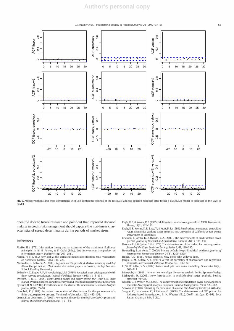
Fig. 5 shows the residuals after fitting the BEKK(2,2) model. In com-parisonwith the original data in Fig. 1, we can see thatmuch of the pre-vious volatility patterns have vanished, this implies that the BEKKmodelwas able to capture the volatility structure of the data set. The au-tocorrelations and cross correlations of the residuals and the squaredresiduals are displayed in Fig. 6. There are no significant auto- andcross correlations left.We conduct portmanteau and Lagrangemultipli-er tests and find no evidence of remaining ARCH effects. Overall, whenconsidering the test results and the autocorrelation and cross correla-tion plots of all three time series, the evidence that our model capturesthe structure in the second order moments of the time series well isvery strong. When conducting the Jarque–Bera test for normality (seeJarque & Bera, 1987), the null hypothesis of normally distributed resid-uals is clearly rejected. Note, that this alone should not be viewed as adrawback of this modeling approach, as the model in Eqs. (1) and (2)is based on white noise in contrast to normal innovations.2

4. Conclusion

In this paper we robustly estimate a vector autoregressive general-ized conditional heteroskedastic VAR-BEKK model with the aim of un-derstanding the development of the dependency structures betweencredit spreads and two major explanatory variables, namely equityreturns and changes in implied volatility. The dynamics of the financialcrisis point out that credit risk is not yet fully understood. Our findings

2 In order to obtain consistency and asymptotic normality of the estimators, strongrequirements such as the existence of the eighth moments of the error distribution(Comte & Lieberman, 2003) are necessary while problematic. This should be kept inmind when considering alternative heavy tailed error distributions.



open the door to future research and point out that improved decisionmaking in credit risk management should capture the non-linear char-acteristics of spread determinants during periods of market stress.

References

Akaike, H. (1973). Information theory and an extension of the maximum likelihoodprinciple. In B. N. Petrov, & F. Csáki (Eds.), 2nd International symposium oninformation theory, Budapest (pp. 267–281).

Akaike, H. (1974). A new look at the statistical model identification. IEEE Transactionson Automatic Control, 19(6), 716–723.

Alexander, C., & Kaeck, A. (2006). Regimes in CDS spreads: A Markov switching model ofiTraxx Europe indices. ICMA centre discussion papers in finance, Henley BusinessSchool, Reading University.

Bollerslev, T., Engle, R. F., & Wooldridge, J. M. (1988). A capital asset pricing model withtime-varying covariances. Journal of Political Economy, 96(1), 116–131.

Byström, H. N. E. (2005). Credit default swaps and equity prices: The iTraxx CDS indexmarket.Working papers. Lund University (Lund, Sweden): Department of Economics.

Byström, H. N. E. (2006). CreditGrades and the iTraxx CDS indexmarket. Financial AnalystsJournal, 62(6), 65–76.

Campbell, K. (1982). Recursive computation of M-estimates for the parameters of afinite autoregressive process. The Annals of Statistics, 10(2), 442–453.

Comte, F., & Lieberman, O. (2003). Asymptotic theory for multivariate GARCH processes.Journal of Multivariate Analysis, 84(1), 61–84.

Engle, R. F., & Kroner, K. F. (1995).Multivariate simultaneous generalizedARCH. EconometricTheory, 11(1), 122–150.

Engle, R. F., Kroner, K. F., Baba, Y., & Kraft, D. F. (1993).Multivariate simultaneous generalizedARCH. Economics working paper series 89–57. University of California at San Diego:Department of Economics.

Ericsson, J., Jacobs, K., & Oviedo, R. A. (2009). The determinants of credit default swappremia. Journal of Financial and Quantitative Analysis, 44(1), 109–132.

Hannan, E. J., & Quinn, B. G. (1979). The determination of the order of an autoregression.Journal of the Royal Statistical Society, Series B, 41, 190–195.

Houweling, P., & Vorst, T. (2005). Pricing default swaps: Empirical evidence. Journal ofInternational Money and Finance, 24(8), 1200–1225.

Huber, P. J. (1981). Robust statistics. New York: John Wiley & Sons.Jarque, C. M., & Bera, A. K. (1987). A test for normality of observations and regression

residuals. International Statistical Review, 55, 163–172.Li, W. K., & Hui, Y. V. (1989). Robust multiple time series modelling. Biometrika, 76(2),

309–315.Lütkepohl, H. (1991). Introduction to multiple time series analysis. Berlin: Springer-Verlag.Lütkepohl, H. (2005). New introduction to multiple time series analysis. Berlin:

Springer-Verlag.Norden, L., & Weber, M. (2009). The comovement of credit default swap, bond and stock

markets: An empirical analysis. European Financial Management, 15(3), 529–562.Schwarz, G. (1978). Estimating the dimension of amodel. The Annals of Statistics, 6, 461–464.Sougné, C., Heuchenne, C., & Hübner, G. (2008). The determinants of CDS prices: An

industry-based investigation. In N. Wagner (Ed.), Credit risk (pp. 85–96). BocaRaton: Chapman & Hall CRC.

0 5 10 15 20 25 30 0 5 10 15 20 25 30 0 5 10 15 20 25 30

0 5 10 15 20 25 30 0 5 10 15 20 25 30 0 5 10 15 20 25 30

00.

40.

8

AC

F it

raxx

AC

F e

uros

toxx

AC

F v

stox

x

00.

40.

8

AC

F it

raxx

^2

AC

F e

uros

toxx

^2

AC

F v

stox

x^2

−0.

50

0.5

CC

F it

raxx

, eur

osto

xx

CC

F it

raxx

, vst

oxx

CC

F e

uros

toxx

, vst

oxx

−20 10 0 10 20

−20 10 0 10 20

−20 10 0 10 20

−20 10 0 10 20

−20 10 0 10 20

−20 10 0 10 20

00.

20.

4

00.

40.

80

0.4

0.8

−0.

50

0.5

00.

20.

4

00.

40.

80

0.4

0.8

−0.

50

0.5

00.

20.

4

CC

F it

raxx

^2, e

uros

toxx

^2

CC

F it

raxx

^2, v

stox

x^2

CC

F e

uros

toxx

^2, v

stox

x^2

Fig. 6. Autocorrelations and cross correlations with 95% confidence bounds of the residuals and the squared residuals after fitting a BEKK(2,2) model to residuals of the VAR(1)model.


author's personal copy - universität passau€¦ · article info abstract ......

Documents