author's personal copy - geometry processing

This article was published in an Elsevier journal. The attached copyis furnished to the author for non-commercial research and

education use, including for instruction at the author’s institution,sharing with colleagues and providing to institution administration.

Other uses, including reproduction and distribution, or selling orlicensing copies, or posting to personal, institutional or third party

websites are prohibited.

In most cases authors are permitted to post their version of thearticle (e.g. in Word or Tex form) to their personal website orinstitutional repository. Authors requiring further information

regarding Elsevier’s archiving and manuscript policies areencouraged to visit:

http://www.elsevier.com/copyright

http://www.elsevier.com/copyright

Author's personal copy

Ultramicroscopy 108 (2007) 29–42

General three-dimensional image simulation and surface reconstructionin scanning probe microscopy using a dexel representation

Xiaoping Qiana,�, J.S. Villarrubiab

aMechanical and Aerospace Engineering, Illinois Institute of Technology, Chicago, IL 60613, USAbNational Institute of Standards and Technology,1 100 Bureau Drive, Stop 8212, Gaithersburg, MD 20899, USA

Received 23 November 2006; received in revised form 17 February 2007; accepted 22 February 2007

Abstract

The ability to image complex general three-dimensional (3D) structures, including reentrant surfaces and undercut features using

scanning probe microscopy, is becoming increasing important in many small length-scale applications. This paper presents a dexel data

representation and its algorithm implementation for scanning probe microscope (SPM) image simulation (morphological dilation) and

surface reconstruction (erosion) on such general 3D structures. Validation using simulations, some of which are modeled upon actual

atomic force microscope data, demonstrates that the dexel representation can efficiently simulate SPM imaging and reconstruct the

sample surface from measured images, including those with reentrant surfaces and undercut features.

r 2007 Elsevier B.V. All rights reserved.

PACS: 82.20.Wt; 83.85.Ns; 87.64.Dz

Keywords: Dilation; Erosion; Mathematical morphology; Atomic force microscopy; Scanning probe microscopy; Dexel representation

1. Introduction

Scanning probe microscopy (SPM) includes atomic forcemicroscopy (AFM), scanning tunneling microscopy (STM)and a number of other variants. It has become one of themost important nano-scale probing and manipulationtools. It provides a vital tool for dimensional measurementof topographic features at nanometer-scale resolution [1].The diminishing feature size in semiconductors and thegrowing academic and industrial research interests in nano-technologies have lead to the widespread use of SPM in avariety of applications. However, conventional SPMinstruments, due to their cone-like probe shape and theunidirectional feedback systems, have their images re-stricted to shapes (‘‘umbras’’) characterized by a singleheight at each lateral position. These instruments cannot

accurately image reentrant or even nearly vertical featuresof specimens. The dimensional characterization of suchreentrant surfaces at the nano-scale, including measure-ments of side-wall angles, side-wall roughness, and widthvariability of lines and trenches, are urgently needed in thesemiconductor industry as feature size is reduced to followthe International Technology Roadmap for Semiconduc-tors [2].For a number of years now, probes with lateral

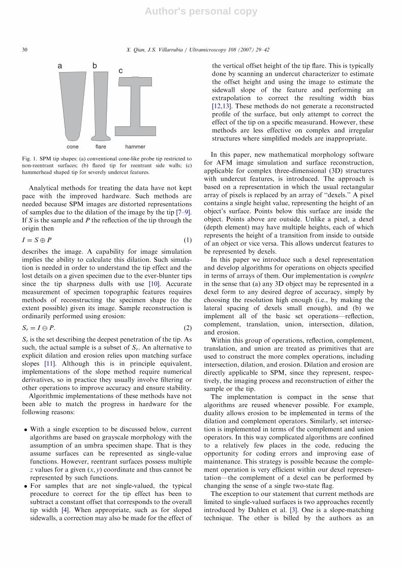
protrusions and feedback systems with bi-directional servocontrol have been incorporated into the newer AFMinstruments [3–6]. In these SPM systems, probes aredesigned with flare- or hammerhead-like shapes to accessreentrant surfaces and undercut features. Fig. 1 gives aschematic description of probe shape extension fromconventional cone-like probe tips restricted to non-reentrant surfaces, to flared tips for reentrant surfaces,and to hammerhead shaped tips for severely undercutfeatures. These instruments, which are capable of imagingundercut features, have found applications as referencemetrology tools at SEMATECH and in a number ofsemiconductor fabrication facilities.

ARTICLE IN PRESS

www.elsevier.com/locate/ultramic

0304-3991/$ - see front matter r 2007 Elsevier B.V. All rights reserved.

doi:10.1016/j.ultramic.2007.02.031

�Corresponding author. Tel.: +1312 567 5855; fax: +1 312 567 7230.

E-mail addresses: [email protected] (X. Qian), [email protected]

(J.S. Villarrubia).1Contributions of the National Institute of Standards and Technology

are not subject to copyright.


Analytical methods for treating the data have not keptpace with the improved hardware. Such methods areneeded because SPM images are distorted representationsof samples due to the dilation of the image by the tip [7–9].If S is the sample and P the reflection of the tip through theorigin then

I ¼ S � P (1)

describes the image. A capability for image simulationimplies the ability to calculate this dilation. Such simula-tion is needed in order to understand the tip effect and thelost details on a given specimen due to the ever-blunter tipssince the tip sharpness dulls with use [10]. Accuratemeasurement of specimen topographic features requiresmethods of reconstructing the specimen shape (to theextent possible) given its image. Sample reconstruction isordinarily performed using erosion:

Sr ¼ I � P. (2)

Sr is the set describing the deepest penetration of the tip. Assuch, the actual sample is a subset of Sr. An alternative toexplicit dilation and erosion relies upon matching surfaceslopes [11]. Although this is in principle equivalent,implementations of the slope method require numericalderivatives, so in practice they usually involve filtering orother operations to improve accuracy and ensure stability.

Algorithmic implementations of these methods have notbeen able to match the progress in hardware for thefollowing reasons:

� With a single exception to be discussed below, currentalgorithms are based on grayscale morphology with theassumption of an umbra specimen shape. That is theyassume surfaces can be represented as single-valuefunctions. However, reentrant surfaces possess multiplez values for a given ðx; yÞ coordinate and thus cannot berepresented by such functions.� For samples that are not single-valued, the typicalprocedure to correct for the tip effect has been tosubtract a constant offset that corresponds to the overalltip width [4]. When appropriate, such as for slopedsidewalls, a correction may also be made for the effect of

the vertical offset height of the tip flare. This is typicallydone by scanning an undercut characterizer to estimatethe offset height and using the image to estimate thesidewall slope of the feature and performing anextrapolation to correct the resulting width bias[12,13]. These methods do not generate a reconstructedprofile of the surface, but only attempt to correct theeffect of the tip on a specific measurand. However, thesemethods are less effective on complex and irregularstructures where simplified models are inappropriate.

In this paper, new mathematical morphology softwarefor AFM image simulation and surface reconstruction,applicable for complex three-dimensional (3D) structureswith undercut features, is introduced. The approach isbased on a representation in which the usual rectangulararray of pixels is replaced by an array of ‘‘dexels.’’ A pixelcontains a single height value, representing the height of anobject’s surface. Points below this surface are inside theobject. Points above are outside. Unlike a pixel, a dexel(depth element) may have multiple heights, each of whichrepresents the height of a transition from inside to outsideof an object or vice versa. This allows undercut features tobe represented by dexels.In this paper we introduce such a dexel representation

and develop algorithms for operations on objects specifiedin terms of arrays of them. Our implementation is complete

in the sense that (a) any 3D object may be represented in adexel form to any desired degree of accuracy, simply bychoosing the resolution high enough (i.e., by making thelateral spacing of dexels small enough), and (b) weimplement all of the basic set operations—reflection,complement, translation, union, intersection, dilation,and erosion.Within this group of operations, reflection, complement,

translation, and union are treated as primitives that areused to construct the more complex operations, includingintersection, dilation, and erosion. Dilation and erosion aredirectly applicable to SPM, since they represent, respec-tively, the imaging process and reconstruction of either thesample or the tip.The implementation is compact in the sense that

algorithms are reused whenever possible. For example,duality allows erosion to be implemented in terms of thedilation and complement operators. Similarly, set intersec-tion is implemented in terms of the complement and unionoperators. In this way complicated algorithms are confinedto a relatively few places in the code, reducing theopportunity for coding errors and improving ease ofmaintenance. This strategy is possible because the comple-ment operation is very efficient within our dexel represen-tation—the complement of a dexel can be performed bychanging the sense of a single two-state flag.The exception to our statement that current methods are

limited to single-valued surfaces is two approaches recentlyintroduced by Dahlen et al. [3]. One is a slope-matchingtechnique. The other is billed by the authors as an

ARTICLE IN PRESS

hammerflarecone

Fig. 1. SPM tip shapes: (a) conventional cone-like probe tip restricted to

non-reentrant surfaces; (b) flared tip for reentrant side walls; (c)

hammerhead shaped tip for severely undercut features.

X. Qian, J.S. Villarrubia / Ultramicroscopy 108 (2007) 29–4230


‘‘erosion’’ algorithm (quotes in original) that ‘‘is not adirect application of erosion in a strict sense’’ because itobtains the outer boundary of a surface rather than acomplete set of points describing the region. It appears tobe a swept volume subtraction method applied to the imagesurface to reconstruct the sample. It was implemented for2D profiles and demonstrated [14] on these to give goodagreement with TEM cross-sections. The method should beextendable to 3D. Despite the authors’ modesty, it appearsto us that Dahlen’s method is a legitimate implementationof erosion for the surfaces that it treats. If it and themethod we present here are both correctly implemented,they should yield the same results. The main distinguishingfeatures of the present work are: (1) The dexel implementa-tion is a rigorous implementation of set-theoretic opera-tors. Because of this we can be certain that the theorems ofset theory and mathematical morphology apply to them.This allows relatively easy building up of more complexoperations out of simple ones. Indeed, we have alreadymade some such extensions. (2) The present implementa-tion is not limited to erosion alone, but as mentioned aboveincludes dilation, union, intersection, and other set opera-tions. (3) The present implementation is already extendedto 3D.

In Section 2, we describe the dexel representation. InSection 3, we provide details of how the dexel representa-tion is used to implement mathematical morphology andset operations. In Section 4 we describe the sense in whichan array of dexels (a 2D regular grid) approximates a realextended object and show that one may make theapproximation as good as needed by choosing the gridspacing fine enough. A pixel is a special case of the moregeneral dexel. We therefore expect agreement between thenew dexel-based algorithms and the existing grayscalemorphology implementation for those cases where both areapplicable. In Section 5 we demonstrate this agreement. Wealso demonstrate that our implementation gives the correctanswer for a calculation on a simple 3D model structure forwhich the correct answer is independently known.

2. The dexel-based representation

2.1. Selection of computer representation

When choosing a data representation for SPM imagingof 3D structures, representation characteristics such asgeometric coverage, compactness, and algorithm efficiencyare the key factors. Lack of sufficient coverage is the reasonfor eliminating grayscale images from consideration—i.e.,such images cannot represent reentrant structures. In thissection we restrict consideration to methods able torepresent general 3D objects. Interestingly, the subject ofsolid modeling for representing such objects is quitemature, and complex set and morphological operationshave also been studied in the solid modeling community.Two common types of 3D representation [15] areconstructive solid geometry (CSG) and boundary repre-

sentation (B-rep). A CSG model is based on the notion thata physical object can be divided into a set of primitives thatcan be combined in a certain order following a set of rules(e.g., simple set operations like union and intersection plustransformations like translation and rotation) to form theobject. These primitives and rules are represented in a treedata structure. A B-rep model stores the boundaryinformation for a solid (e.g., vertices, edges, and faces,together with the information on how they are connected).Alternatively, a solid can be described by dividing spaceinto a 3D regular grid. Then a 3D array of ones and zeros(for example) can designate which volume elements (orvoxels) in the grid are inside the object and which outside.An octree representation is a tree data structure in whichspace is recursively subdivided into octants. This is similarto a voxel representation except that volume elements arenot all of equal size, so some parts of an object (e.g., theinterior) may be described with a coarse representationwhile others (e.g., near a boundary) may be described witha higher resolution.Solid modeling has become a mature discipline, in which

various computer representations and corresponding mod-eling algorithms that can model general 3D solids havebeen thoroughly studied. Thus, the objective of this paperis not to develop a novel computer representation forgeneral 3D solid modeling, but rather to adapt one to themathematical and computational requirements intrinsic tothe particular application we have, i.e., SPM imaging, andto identify the appropriate computer representation andalgorithms.The morphological operations for SPM imaging are

analogous to modeling operations in swept volume-basedsimulation software for numerical controlled (NC) machin-ing path generation, even though the dilation operation israrely used in NC simulation. The SPM probe movementforming a swept volume is analogous to robotics and NCcutting motion. In NC path generation, software simula-tion is needed to verify the cutting path, to avoid collisionand gauging, and to examine the resulting surface shapeand accuracy in comparison to the nominal surfacegeometry. NC path simulation has received tremendousresearch. The simulation methods include accurate ap-proaches [16,17] or and approximate methods [18].The approaches based on CSG and B-rep are theoreti-

cally capable of providing accurate NC milling simulationand verification. However, they are computationallyintense. The cost of simulation is reported to be OðN4Þ,where N is the number of tool movements [19]. A complexNC program can consist of thousands of motion steps.SPM imaging can consist of hundreds of thousandsmovements, making such computation even more intract-able.The approximate methods have OðNÞ computational

complexity and they include the voxel-based approach,dexel (depth element) approach, and octree approach[20,21]. The voxel representation is easy to implement butrequires larger storage space. In comparison, the dexel [22]

ARTICLE IN PRESSX. Qian, J.S. Villarrubia / Ultramicroscopy 108 (2007) 29–42 31


is a version of run length encoded volumetric datarepresentation where 3D objects are represented as a setof 1D blocks with depth on a grid. Since this is therepresentation we chose, details will be provided below.The dexel and its variants have been widely used in avariety of NC simulation systems [18,22,23].

Table 1 gives a comparison of the suitability of various3D computer representations for morphological represen-tation. The comparison items include:

� Ease of creation: whether the initial 3D representationcan be easily created from SPM imaging data. Thecreation of CSG and B-rep from SPM data involves thereconstructing higher order analytical surfaces fromSPM data.� Accuracy: whether the 3D representation can accuratelyrepresent various specimen and tip shapes. Neither voxelnor dexel represent analytical surfaces exactly. However,through controlling the sampling resolutions, they canrepresent the SPM image data with the same accuracy asB-rep.� Efficiency: whether the 3D representation supportsefficient morphological operations. Both CSG and B-rep have OðN4Þ computational complexity and dexel hasOðNÞ, where N is the number of SPM imaging points.� Compactness: whether the 3D representation can repre-sent an arbitrarily shaped specimen in a compactmanner. CSG representation can compactly representan object through a series of set operations. Thecompactness of B-rep of a nanostructure from SPMmeasurement depends on the object and the requiredaccuracy. To maintain representation accuracy, bothdexel and voxel need larger number of cells. However,dexel is more efficient in z-axis since it uses the runlength encoded representation.� Ease of coding: whether the 3D representation and thecorresponding morphological operations can be easilycoded.� Compatibility: whether the proposed 3D representationis compatible with grayscale morphological operationsin conventional SPM imaging systems. The conversionof an umbra into a voxel requires the unnecessaryassumption of a bottom for each pixel height.

It is clear from Table 1 that there is no single representationthat is excellent in all aspects. CSG and B-rep are poor incomputing efficiency and in initial model creation since

they require the explicit definition of surfaces from SPMimages and probe data. The Boolean operations for B-repare also challenging in terms of coding. However, they cancompactly and accurately represent 3D specimen andprobe shape. On the other hand, voxel representation ispoor in terms of representation compactness since itinvolves discretizing the sample object in all three dimen-sions. However, it is easy to code, the initial model creationis easier, and the modeling algorithms are efficient. Thedexel representation is a run length encoded version ofvolumetric data representation and is more compact andmore accurate than voxel.Therefore, we adopted dexel representation in our

implementation of mathematical morphology softwarefor general 3D structures.

2.2. Dexel-based representation

The dexel approach is a version of volumetric datarepresentation where 3D objects are represented as a set of1D blocks with depth on a grid. It is more compact andmore accurate than voxel since it does not involve thediscretization in the z-dimension.We may construct a dexel object, Ad, associated with a

real object A, as follows. First choose an origin andorientation for a rectangular coordinate system. Define agrid in the x–y plane of this coordinate system. The x

coordinates in this grid are given by xi ¼ x0 þ idx for i ¼

0; 1; . . . ;mx � 1 with i an integer index, mx the number ofgrid elements in the x direction, x0 the position of the firstsuch element, and dx the grid spacing in the x direction.The y coordinates are similarly defined. Now imagine aline, Lij (with z ranging from �1 to 1) at xi; yj for eachi; j in the grid. We can define Ad as

Ad ¼[i;j

ðLij \ AÞ. (3)

A 2D example of this is shown in Fig. 2. The object(shown gray) has undercut edges. Those intervals of thelines that are enclosed by the object are shown darker. Thedexel object representation includes the collection oflocations of the endpoints of these intervals in an indexedgrid. Each column in the object is represented by a singledexel. The entire object is then a 2D array of dexels.To support a complete set representation we allow �1

and1 as possible initial and final heights in a dexel. This isnecessary, for example, to represent the complement of abounded set, since such a complement will be unbounded.

ARTICLE IN PRESS

Table 1

Representation comparison

3D representation Ease of creation Accuracy Efficiency Compactness Ease of coding Compatibility

CSG N Y N Y N N

B-rep N Y N ? N N

Voxel Y Y Y N Y ?

Dexel Y Y Y ? Y Y



It is also desirable because it makes the umbra interpreta-tion of SPM data that is used in grayscale morphology aspecial case of the dexel representation.

Formal representation properties of dexel, as noted in Ref.[24], include spatial addressability and spatial hashing,directionality, Boolean simplification, rigid motion, discretetranslations, null-set representation, and completeness.

2.3. Data structure

Our dexel data structure is illustrated in Fig. 3. The datarepresentation consists of a flag and a linked list of zero ormore heights. (Absence of any heights would be indicatedby a null list.) The flag may take on two values, ‘‘inside’’ or‘‘outside,’’ which may be represented by �1=1, 0=1,Boolean true/false, or any other convenient pair. The valueof this flag indicates whether the starting position at z!

�1 is inside or outside the dexel. The heights in the heightlist are ordered from smallest to largest. The sense ofinside/outside toggles back and forth at each height. Theinside/outside state after the last height in the list isconsidered to remain in effect as z!1.

Following are some examples:

� The dexel fflag ¼ inside; HeightList ¼ f10gg representsthe interval ð�1; 10�. (The starting position at �1 isinside, and the single height in the height list thereforerepresents an inside to outside transition.) This isequivalent to a pixel with value 10 in the umbrainterpretation of an image.� The dexel fflag ¼ inside; HeightList ¼ f0; 1; 3gg repre-sents the union of intervals ð�1; 0� and [1,3].� If the last height were omitted, there would be no finaltransition from inside to out. That is, fflag ¼inside; HeightList ¼ f0; 1gg represents the union ofintervals ð�1; 0� and ½1;1�.� fflag ¼ outside; HeightList ¼ f0; 1gg represents the in-terval ½0; 1�.� fflag ¼ inside; HeightList ¼ fnullgg represents the uni-versal set ð�1;1Þ. (We start inside and there is notransition to outside.)

� fflag ¼ outside; HeightList ¼ fnullgg represents the nullset. (We start outside and there is no transition toinside.)

Just as an image is a 2D array of pixels, a dexel object in itssimplest form is a 2D array of dexels. Additionalinformation may be included if desired. For example, ourimplementation includes data structures to represent thelateral coordinates of the dexel at the 0,0 position and thelateral grid spacing (which we called dx and dy above).

2.4. Advantages of the data structure

There are two basic advantages of our data structure.

1. It easily represents umbra objects and objects withundercuts. By allowing dexel intervals to extend to �1it allows representations of the null or universal sets,and it allows the complement of any set to berepresented. The infinity value is represented logi-cally—it is implicit in the flag and number of heightvalues in the list—instead of as an explicit number (e.g.,the maximum or minimum number of which thecomputer is capable) stored as a boundary height. Thismakes the representation compatible with any of thecommon data types on a computer that have no explicitrepresentation for �1. (Simply using a large magnitudenumber to represent �1 in such a data type is machine-dependent and can lead to overflow during dilation orerosion.)

2. The second advantage of such representation is theefficiency of the set-theoretic complement operation.The complement of a dexel is obtained by toggling itsflag from inside to outside or vice versa. The rapidity ofthis operation makes it possible to develop only twobasic operations: union and dilation. All other setoperations can be efficiently obtained as described in thenext section using the complement operation andduality. This also makes the code compact and robust.

3. Set and morphology operations on dexel-represented

objects

3.1. General considerations

We build the set and morphological operations on a fewprimitive operations: dexel complement, dexel union andblock–block dilation. All other set operations such asintersection and subtraction, and dilation and erosionoperations between dexel objects are derived from thesethree.

ARTICLE IN PRESS

hh h ... h null

Flag

Fig. 3. Dexel data structure: linked ordered height list.

Fig. 2. Dexel representation of an object.

X. Qian, J.S. Villarrubia / Ultramicroscopy 108 (2007) 29–42 33


The usual erosion and intersection operations may leadto dangling boundaries. For example, the intervals ½�1; 0�and ½0; 1� overlap at the single point, f0g, on the boundaryof both. If we were strict we would therefore need to keepcareful track of whether each dexel height value in theheight list represents the boundary of an open or closedinterval. This would increase the complexity of theimplementation without a compensating reward—in a realSPM a ‘‘0-width’’ feature (if such a thing could exist) woulddoubtless be broken unobserved by any tip that madecontact with it. Nothing is lost by forbidding such features,since any actual small feature can still be represented by asmall but finite size. We therefore implement regularized setoperations [15]. Regularization closes intervals to theinterior—so e.g., ð0; 5Þ becomes ½0; 5�—and prunes awayboundaries that are not associated with any interior region(like the single f0g in our first example). Among otherconveniences, this choice insures that the set and morpho-logical operations have the closure property. That is, theresulting object after the set and morphological operationsremains a valid object in dexel representation and canparticipate in subsequent set operations.

3.2. Primitive set operations

3.2.1. Dexel complement

The dexel complement is accomplished by toggling thevalue of the dexel flag. Since the sense of inside/outsidetoggles at each boundary this changes all inside–outsidetransitions into outside–inside transitions and vice versa.Within the conventions of regularized set operations(where boundaries are closed) this is exactly what is meantby the complement. So, for example, the interval ½a; b� isexpressed in dexel form as foutside; fa; bgg. Its regularizedcomplement is ð�1; a� [ ½b;1Þ, which in dexel form isfinside; fa; bgg.

3.2.2. Dexel–dexel union

A simple model of dexel–dexel union is illustrated inFig. 4. Imagine the two dexels, A and B positioned side byside as shown. Let the ‘‘depth’’ inside A at position z be 1 ifz is contained in A and 0 otherwise. The depths inside A

and B are ‘‘projected’’ onto the screen at the right, whichrecords their sum. The sum may be 0, 1, or 2. Obviously thedepth inside C ¼ A [ B must be 0 when the depth on thescreen is 0 (z is outside both A and B) and 1 otherwise (i.e.,when the total depth is 1 or 2, indicating z is inside one orboth of A and B). Changes in the total depth obviously canonly happen at the z values in the height lists of A and B.

To construct an efficient algorithm to implement thisscheme, the initial depths in A and B are set to 0 or 1depending upon whether their flag values are outside orinside. The total depth is initialized to the sum of these. Thevalue of C’s flag is set to outside if this sum is 0, inside if itis 1 or 2. One then iterates up the two height lists. At eachiteration, one examines the next available heights from thetwo lists. The smaller of the two is drawn from its list, the

corresponding depth is updated, and the total depth isupdated. (If the two heights happen to be the same, theyare both drawn and all depths are updated.) If the totaldepth changes from nonzero to zero or from zero tononzero, the drawn height is saved in C’s list. (It representsa transition in C from inside to outside or vice versa.)Otherwise it is discarded. When a list runs out of heights, itis treated as though its next height is 1. That is, oneproceeds by always drawing heights from the remaining listuntil it too is exhausted.

3.2.3. Block–block dilation

Each dexel can be thought of as the union of a number ofintervals, or ‘‘blocks,’’ each of which is specified by itslower and upper boundaries. One of these blocks is labeledin Fig. 2. In terms of these blocks the dexel object, Ad,defined in Eq. (3) can also be written as

Ad ¼[i;j

[k

bijk

!, (4)

where i and j are the grid indices, and k indexes the blockswithin each dexel.This is a useful conceptual formulation because the

dilation of two blocks is particularly simple. We use thefollowing definition of dilation:

A� B ¼[b2B

ðAþ bÞ, (5)

where Aþ b with A a set and b a vector is defined by

Aþ b ¼ faþ bja 2 Ag. (6)

That is, it is the set obtained by translating every point in A

by b. When A and B are both blocks, denoted by ½hi; hiþ1�

ARTICLE IN PRESS

Fig. 4. Dexel–dexel union through keeping track of inside/outside status

change.



and ½hj ; hjþ1�, their dilation is another block:

½hi; hiþ1� � ½hj ; hjþ1� ¼ ½hi þ hj ; hiþ1 þ hjþ1�. (7)

3.3. Set operations on objects comprised of dexels

The above primitive operators can be used in combina-tion to generate operators for dexel-represented objects.Reflection, complement, union, intersection and subtrac-tion are straightforward. They also form the basis of twoalgorithms that will be directly applied for SPM imagesimulation and surface reconstruction: dilation and ero-sion.

The reflection of a set, A, denoted �A, replaces everyvector a 2 A by �a. A dexel object consists of a 2D arrayof dexels. The lateral (x–y) coordinates of the reflection areaccomplished the same way it is done for an image—theorder along both axes is reversed. Each dexel must thenalso be reflected in the z-direction. This is done bymultiplying all heights in the height list by �1 andreversing their order (so they are once again in increasingorder). If there are an odd number of heights in the list, theflag must be toggled.

The complement of a dexel object is formed by takingthe complement of all the dexels forming the object.

If two dexel objects are defined on the same grid, eachgrid point will be associated with one dexel from eachobject. The union is formed by forming the dexel unions ateach grid coordinate using the dexel–dexel union procedureof the last section.

Intersection is computed by means of DeMorgan’s lawusing the already described union and complementprimitives:

A \ B ¼ ðAc [ BcÞc. (8)

Set subtraction, A� B, removes from A all parts containedin B. Subtraction is implemented as

A� B ¼ A \ Bc ¼ ðAc [ BÞc. (9)

The first form is simplest. The second, obtained byapplying DeMorgan’s law to the first, is expressed in termsof the union and complement primitives.

Dilation may be implemented in steps. Since the dilationprimitive defined above is for block–block dilation, the first(and only new) step is to implement dilation of two dexels.We can think of a dexel as a union of blocks so that if adexel D has n blocks and D has m

D ¼[ni¼1

Di,

D ¼[mj¼1

Dj, ð10Þ

Di, i ¼ 1; . . . ; n are D’s blocks and similarly for D. It is ageneral property of dilation that

ðA [ BÞ � C ¼ ðA� CÞ [ ðB� CÞ. (11)

See for example Ref. [25, proposition 15]. Using thisrule, the dilation of dexels D and D defined by Eq. (10) canbe written as the union of dilations of blocks.

D�D ¼[ni¼1

Di �[mj¼1

Di ¼[i;j

ðDi �DjÞ, (12)

where the final union is over all pairings of blocks in thetwo dexels. The dilations on the right side of Eq. (12) are allinstances of the previously defined block–block dilationprimitive, and unions of blocks are a special case of theunion of dexels primitive. Hence Eq. (12) defines dex-el–dexel dilation in terms of operations we already knowhow to do.The second step is to define dilation of the 2D arrays of

dexels that comprise dexel objects. This part is completelyanalogous to grayscale dilation of images. (See Ref. [8,Appendix C].) In grayscale dilation, pixel–pixel dilationamounts to a single sum—the upper interval bound in Eq.(7)—since for pixels there is never more than one block,and that block’s lower bound is always �1. The union oftwo pixels is a pixel with value equal to the maximum ofthe two input values. Dilation of dexel objects can use thesame algorithm except that the sum (pixel dilation) isreplaced by dexel dilation as in Eq. (12), and the maximum(pixel union) is replaced by dexel union as described inSection 3.2.The erosion operation between two dexel objects is done

using dilation based on their duality property Ref. [25,Theorem 25]:

A� B ¼ ½Ac � ð�BÞ�c. (13)

4. Discussion

As defined above, we can think of a dexel as a set ofintervals along a line. Like a line, the dexel has extent inonly one dimension. It has no width. This is a useful featureinasmuch as the dilation of two columnar objects, eachwith width w, is an object with width 2w. Consequently, ifwe attempted to associate some nonzero fixed width withdexels, the dilation of one dexel with another would notproduce a dexel, but rather an object two dexels wide. Bydefining dexels to have no width, this is avoided; closure ofdilation and erosion with respect to dexels is preserved.This choice is analogous to the usual convention with pixel-represented objects. In grayscale morphology pixels arealso commonly treated as having height but no width forthe purpose of computing dilation and erosion.As computationally convenient as this may be, it

nevertheless raises questions about the sense in which adexel or pixel representation can approximate a real object.Fig. 5 illustrates the problem. Suppose the curved solid linelabeled A represents the boundary of an extended object.The dexel object, Ad, associated with A is an array of dexelson a regularly spaced grid. This is represented by the thickvertical line segments. Ad differs from A inasmuch as the

ARTICLE IN PRESSX. Qian, J.S. Villarrubia / Ultramicroscopy 108 (2007) 29–42 35


space between dexels is not filled—its total volume is 0.Furthermore, as we have just discussed, dilation of realobjects results in an object of width greater than either ofthe original objects alone. Is some part of this widthincrease neglected due to the treatment of dexels as havingno width? Intuitively, it seems that the importance of theseconcerns should diminish as the grid spacing grows finer.In the following discussion, we sketch one way thisintuitive insight might be placed on a firmer footing.

Define an object, R, to be a horizontal rod of length r inthe x direction (left to right in Fig. 5). We consider itsorigin to be at its center. Then defineeA ¼ Ad � R. (14)

If we choose r to be the grid spacing in the x direction, theneA is as shown in the figure. The dilation sweeps each dexelby r=2 to the left and right. The occupied intervals in eachdexel, originally 0-width line segments, are widened by thisprocedure into rectangular blocks that span the full widthof the grid cell occupied by the dexel. This closes the gapsbetween dexels and widens the object by r=2 on each side.

We chose to define the individual blocks within Ad suchthat the blocks coincide with the intersection of grid lineswith A, as described in Section 2.2. That is, the boundariesof the blocks in Ad coincide with the boundaries of A. Withthis choice Ad � A. Dilation is increasing with respect toboth its arguments. See, e.g., Proposition 12 and Corollary13 in Ref. [25], which says that

A � B implies A�D � B�D. (15)

(Dilation is commutative, A� B ¼ B� A, so the increas-ing property stated here for the first argument appliesequally well to the second.) Since Ad � A this propositionmeans in the present case that Ad � R ¼ eA � A� R. ThuseA is bounded above by an object that differs from A onlyby something on the order of the grid size. It is similarlybounded below. Since the blocks in Ad terminate exactly on

the boundary of A, the same argument can be made withrespect to the complements of eA and A, leading to theresult that eAc � Ac � R. Since R is symmetrical ðR ¼ �RÞ,Eq. (13) then implies eAc � ðA� RÞc, or eA A� R. Theupper and lower bounds are summarized as

A� R � eA � A� R. (16)

Now suppose we choose finer and finer grid spacings forour description. As r! 0 the horizontal rod, R, ap-proaches a single point, {0}, so A� R and A� R both tendto A. eA is squeezed between outer and inner bounds that inthis limit both approach the same value (A), and thereforeeA! A. It is in this sense that eA is an approximation for A.It can be made as close to A as desired by choosing the gridspacing fine enough.Similar relationships hold if we use these dexel-approxi-

mated sets to calculate objects that are interesting for SPM.Given a sample, S, and tip, P, the image is given by

I ¼ S � P. (17)

Suppose we approximate S and P as dexel objects dilatedwith R as in Eq. (14), so that S � R � eS � S � R andP� R � eP � P� R. We can then compute an approx-imate image according toeI ¼ eS � eP. (18)

Because dilation is increasing with respect to both inputs,we can derive lower and upper bounds for eI by replacing eSand eP in Eq. (18) with their lower and upper bounds

ðS � RÞ � ðP� RÞ � eI � ½S � R� � ½P� R�. (19)

The bounds on eI are not as tight as those on A in Eq. (16).There are two appearances of R on each side instead ofonly one. This is owing to the fact that both inputs eS and ePwere approximate.The other calculated quantity of interest to us here is the

reconstructed sample from the measured image, I, and aknown tip shape P. This reconstruction is formed byerosion:

Sr ¼ I � P. (20)

If we define the approximation eSr ¼ eI � eP one can findupper and lower bounds similarly to the previousexamples. The only difference is that eI � eP is increasingin eI and decreasing in eP, so the upper bound of eSr must beformed by using the upper bound of eI and the lower boundof eP while the opposite is done to form the lower bound. Inthis way one arrives at

ðI � RÞ � ðP� RÞ � eSr � ðI � RÞ � ðP� RÞ. (21)

Eqs. (19) and (21) behave similarly to Eq. (16) as r getssmall, in the sense that the upper and lower bounds bothapproach the true value of the object we are approximat-ing. In all cases the approximation can be made as close asone likes by choosing the grid spacing fine enough.This discussion was limited to a 2D example for

simplicity and ease of illustration. However, it is equally

ARTICLE IN PRESS

Fig. 5. The sense in which a dexel object approximates a real one. The

dexel object Ad consists of an array of dexels (the thick vertical bars), each

terminating on the real object, A, it is intended to approximate. Dilation

by a horizontal grid element, R, expands Ad into rectangular blocks ( eA,

shown with thinner lines). eA is bounded above and below by A�R (outer

dashed) and A�R (inner dashed) as shown.



applicable in 3D. The only difference is that instead of ahorizontal rod, R must be a horizontal rectangular elementwith dimensions rx and ry equal to the 2D grid size.

As a consequence of this discussion, we see that theerrors associated with the discreteness of the representationare initially of the order of the grid spacing. Errorsmay accumulate to a few times larger than thisduring calculations. One should choose a grid spacingsmall enough that the associated uncertainties aresmaller than those associated with other sources oferror. With this choice, the dexel-represented objectscan for all practical purposes be substituted for thereal ones.

5. Validation using test data

Note that in all the examples below, the simulated AFMimages were obtained through the dexel dilation operation,as presented in this paper. All the reconstructed samplesurfaces were obtained through the dexel erosion opera-tion.

The data files in these examples are in the dexelrepresentation. Even though the actual AFMs capable ofbi-directional servo control and imaging undercutfeatures may have the output format as ðx; zÞ pairs, it isnot difficult to convert such pairs into the dexel representa-tion through various interpolation methods, such as linearinterpolation.

5.1. Validation for surfaces without undercut features

We first show examples that demonstrate the consistencybetween the new dexel-based method and grayscalemathematical morphology-based method [8] for a set ofsurfaces without undercut features. A grayscale- or umbra-represented object is a special case of a dexel-representedone, in which the dexel at index ði; jÞ has only a singleblock, ð�1; hij � with hij the value of the pixel at index ði; jÞ.Consistency of the methods requires that given equivalent

inputs, the results will be representations of the identicaloutput.

Example 1. Fig. 6 shows an SPM image simulation andsurface reconstruction for a 2D profile based on the newsoftware. The set of translated probes graphically illus-trates the dilation and erosion relations among the trueprofile, SPM image, and reconstructed profile. Thesimulation is done through the dilation of the 2D profilewith a parabolic tip. The reconstruction is obtainedthrough the erosion of the simulated SPM image by thetip. The profile is a cross-section of a rough phosphor thinfilm (more in Example 3).

As expected [8], the reconstructed surface approximatesand correctly bounds the specimen surface. Both thedilation and erosion results are identical to those fromthe grayscale morphology software.

Example 2. Fig. 7 shows an AFM image simulation andsurface reconstruction for a spike surface. For this simplestructure the dexel and grayscale software producedidentical results.

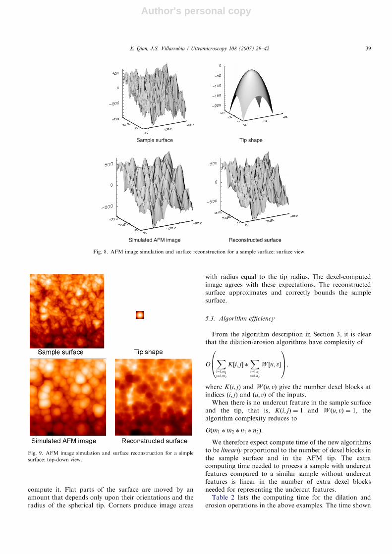
Example 3. The structure labeled ‘‘sample’’ in Figs. 8 and 9is actually an AFM image, available from a previous study[26], of a rough phosphor thin film. For the purpose of thistest we pretend this represents the actual surface of a roughsample. In this way we generate a test in which the samplehas a more realistic variety of structures than in theprevious test. An image is simulated by dilating the samplewith a parabolic tip, as shown. The sample is thenreconstructed by erosion of the tip from the simulatedimage. The reconstructed surface differs from the originalone due to information loss in the dilation process (aknown phenomenon). The new dexel algorithms and theolder grayscale algorithms produced identical results forthe simulated image and reconstructed surfaces in this test.

Thus, the new mathematical morphology software basedon dexel representation supports image simulation and

ARTICLE IN PRESS

0 100 200 300 400

X(nm)

−600

−400

−200

0

200

400

600

Tip Surface

Rcon Surface Image

0 100 200 300 400

X(nm)

−400

−200

0

200

400

600

800

Z(n

m)

Tip Surface

Image

Fig. 6. SPM image simulation and surface reconstruction through morphological operations for a 2D profile. (a) SPM image formation through

morphological dilation, (b) specimen surface reconstruction through morphological erosion.



surface reconstruction for structures without undercutfeatures.

5.2. Validation for surfaces with undercut features

The dexel method is also capable of simulating the SPMimaging of undercut structures and capable of reconstruct-ing the specimen surface of undercut shapes. Since thiscannot be accomplished in grayscale morphology, theexisting software cannot be used for validation as was donein the last section. Instead we use two other methods, oneeach in Examples 4 and 5.

Example 4. In Fig. 10 are pictures of image simulation andsurface reconstruction for a profile with undercut areas.They are obtained through the dilation and erosionoperations by a tip of undercut shape. As Fig. 10ademonstrates, the envelope of the translations of thereflected tip forms the SPM image. As shown in thefigure, if dilation is correctly implemented the tip shouldjust touch the simulated image and not go beyond it whenthe tip apex point is translated to any point along theundercut profile. Likewise, if erosion is properly imple-mented the tip should touch the reconstructed surfacewithout penetrating beyond it when tip moves along the

simulated image. Satisfaction of these requirements wasmanually verified for a large number of points along roughand realistic profiles like the one shown. As expected, thereconstructed surface approximates and bounds theoriginal surface.

Example 5. Fig. 11 shows an artificial sample surface,simulated AFM data through dilation with a spherical tip,and the reconstructed surface through erosion for a 3Dstructure with undercut features. Each 3D surface is shownin two views (x and y cross-sections) and a 3D rendering.To further validate the correctness of the dilation/erosion operation, cross-sectional examination is con-ducted. Fig. 12 shows a cross-section of the dilation/erosion operation for this 3D structure and the overlay ofimage, true surface and reconstructed surface. As the figuredemonstrates, the probe at the image point just touches thesurface but not coincide with the sample surface due to thefinite dimension of the tip. However, the tip shapecoincides exactly with part of the reconstructed surface.The artificial sample used in for this test was deliberatelychosen to be simple—with cross-sections composed ofstraight lines meeting at sharp corners. For this kind ofsimple sample, the result of dilation with a spherical tip iseasy to anticipate even without a dexel-based algorithm to

ARTICLE IN PRESS

Reconstructed surfaceSimulated AFM image

Sample surface Tip

Fig. 7. AFM image simulation and surface reconstruction for a spike surface (Note: the tip is scaled differently from the surface to give a clear illustration

of the tip shape).



compute it. Flat parts of the surface are moved by anamount that depends only upon their orientations and theradius of the spherical tip. Corners produce image areas

with radius equal to the tip radius. The dexel-computedimage agrees with these expectations. The reconstructedsurface approximates and correctly bounds the samplesurface.

5.3. Algorithm efficiency

From the algorithm description in Section 3, it is clearthat the dilation/erosion algorithms have complexity of

OXi¼1;m1j¼1;m2

K ½i; j� Xu¼1;n1v¼1;n2

W ½u; v�

0B@1CA,

where Kði; jÞ and W ðu; vÞ give the number dexel blocks atindices ði; jÞ and ðu; vÞ of the inputs.When there is no undercut feature in the sample surface

and the tip, that is, Kði; jÞ ¼ 1 and W ðu; vÞ ¼ 1, thealgorithm complexity reduces to

Oðm1 m2 n1 n2Þ.

We therefore expect compute time of the new algorithmsto be linearly proportional to the number of dexel blocks inthe sample surface and in the AFM tip. The extracomputing time needed to process a sample with undercutfeatures compared to a similar sample without undercutfeatures is linear in the number of extra dexel blocksneeded for representing the undercut features.Table 2 lists the computing time for the dilation and

erosion operations in the above examples. The time shown

ARTICLE IN PRESS

Sample surface Tip shape

Reconstructed surfaceSimulated AFM image

Fig. 8. AFM image simulation and surface reconstruction for a sample surface: surface view.

Fig. 9. AFM image simulation and surface reconstruction for a simple

surface: top-down view.



in the table is recorded from the tests on a PC (DellOptilex GX520, Pentiums CPU3.40GHz, 1.99GBRAM).2 The sample size and tip size are also shown inthe table.

ARTICLE IN PRESS

0 100 200 300 400 500

nm

0

100

200

300

0

Tip Surface

Rcon Surface Image

0 100 200 300 400 500nm

0

100

200

300

400nm

Tip face

Image

Tip

Rcon Imag

Surf40

Fig. 10. Image simulation and surface reconstruction for a profile with undercut features. (a) Dilation in image simulation, (b) erosion in surface

reconstruction.

Fig. 11. Image simulation and surface reconstruction for a 3D structure with undercut surfaces, showing cross sections through x (left column) and y

(middle column) and a solid rendering (right column). (a) Sample surface, (b) simulated AFM data, (c) reconstructed surface.

2Commercial equipment is identified in order to specify the measure-

ment procedure. Such identification does not imply recommendation or

endorsement by the National Institute of Standards and Technology, nor

does it imply that the equipment identified is necessarily the best available

for the purpose.



A comparison has been made between dexel-based andgrayscale mathematical morphology software for struc-tures without undercut features. The time for Example 1 isnot shown here since its time lapse is very small (0.04 s) forboth software. Our present dexel-based implementation isabout 3 to 5 times slower than the grayscale morphologymethod. At least some part of this difference is theinevitable consequence of a more general procedure. Ingrayscale morphology only the upper of the two bounds inEq. (7) need be calculated. The lower bound is always �1.Even when a dexel object consists of only dexels with asingle block each, the dexel algorithm still must determinethe lower boundary of this block–block dilation, since itcan in general be other than �1. The dexel code must alsocheck for the presence of additional blocks, even if in aparticular case they do not happen to be present.Considering the simplicity of the grayscale block dilation(sum) and union (max) functions, this inevitable overheadmight contribute a factor of 2 or 3 to execution time of themore general algorithm. This suggests that some other partof our observed speed difference might still be improved bymore efficient implementation.

The run times for structures with undercut features as inExamples 4 and 5 are also shown in the table. Thecomparison between Examples 3 (without undercut) and 5(with undercut) demonstrates that the existence of under-cut features only contributes marginally to the dilation/erosion operation time for typical samples. This is becausethe number of undercut dexels is usually only a smallproportion of the overall dexels in Example 5. In Example5, there are total 165 760 blocks for the 400 400 grid in thedilation and 166 068 blocks for the 400 400 grid in erosionoperation.

6. Conclusions

This paper presents a dexel computer representation andits algorithm implementation for SPM image simulationand surface reconstruction on general 3D structures.Experimental validation on both simulated and actualAFM data demonstrates that the dexel representation canefficiently simulate and reconstruct various 3D structures,including those with reentrant surfaces and undercutfeatures.Our contribution in this paper is threefold:

� A dexel-based object representation and its implementa-tion for mathematical morphology are introduced. Therepresentation provides an efficient and compact repre-sentation for general 3D structures, including undercutfeatures.� The implementation is complete in the sense that (a) any3D object may be represented in a dexel form to anydesired degree of accuracy, simply by choosing theresolution high enough, and (b) we implement all of thebasic set operations—reflection, complement, union,intersection, subtraction, dilation, and erosion.� We fulfill a need that has become increasingly importantin semiconductor industry: how to reconstruct surfacesand simulate images of undercut features in SPM.

References

[1] J.E. Griffith, D.A. Grigg, J. Appl. Phys. 74 (9) (1993) 83.

[2] International Technology Roadmap for Semiconductors, Semicon-

ductor Industry Association, San Jose, CA, 2003.

[3] G. Dahlen, M. Osborn, N. Okulan, W. Foreman, A. Chand, J.

Foucher, J. Vac. Sci. Technol. B 23 (6) (2005) 2297 (Also in Veeco

Application Notes AN83-091404).

[4] Y. Martin, H.K. Wickramasinghe, Appl. Phys. Lett. 64 (19) (1994)

2498.

[5] T. Morrison, C. Marotta, Micro Magazine, August/September

(2005).

[6] R. Kneedler, S. Borodyansky, L. Vasilyev, D. Klyachko, A.

Buxbaum, T. Morrison, Proc. SPIE 5567 (2004) 905.

[7] G.S. Pingali, R. Jain, Restoration of scanning probe microscope

images, in: Proceedings of the IEEE Workshop on Applications of

Computer Vision, 1982, p. 282.

[8] J.S. Villarrubia, J. Res. Nat. Inst. Stand. Technol. 102 (4) (1997) 425.

[9] J.S. Villarrubia, Surf. Sci. 321 (1994) 287.

ARTICLE IN PRESS

Fig. 12. A cross-section and an overlay of 3D structures in Fig. 11. (a) Cross-section of dilation and erosion operation, (b) overlay of surface, image,

reconstructed surface.

Table 2

Execution time comparison

Example 2 Example 3 Example 4 Example 5

Software Dexel Grayscale Dexel Grayscale Dexel Dexel

Sample size 101 101 400 400 500 1 400 400

Tip size 31 31 31 31 31 1 31 31

Dilation (s) 0.34 0.11 7.78 1.31 0.05 9.06

Erosion (s) 0.36 0.11 8.00 1.33 0.05 10.25



[10] G. Varadhan, W. Robinett, D. Erie, R.M. Taylorr II, Fast simulation

of atomic-force-microscope imaging of atomic and polygonal

surfaces using graphics hardware, in: SPIE Conference on Visualiza-

tion and Data Analysis, 2002.

[11] D. Keller, Surf. Sci. 253 (1991) 353.

[12] N.G. Orji, R.G. Dixson, Meas. Sci. Technol. 18 (2007) 448.

[13] N.G. Orji, R.G. Dixson, A. Martinez, B.D. Bunday, J.A. Allgair,

T.V. Vorburger, Journal of Micro/Nanolithography, MEMS and

MOEMS, in press.

[14] G. Dahlen, M. Osborn, N.-C. Liu, R.W. Jain, W. Foreman, R.

Osborne, Proc. SPIE 6152 (2006) 61522R-1.

[15] A.A.G. Requicha, Comput. Surv. 12 (4) (1980) 438.

[16] K.C. Hui, Visual Comput. 10 (1994) 306.

[17] W.P. Wang, K.K. Wang, IEEE Comput. Graphics Appl. 6 (12)

(1986) 8.

[18] Y. Huang, J.H. Oliver, NC milling error assessment and tool path

correction, in: Computer Graphics Proceedings, Conference Proceed-

ings July 24–19, 1994, (Proc. SIGGRAPH ’94), 1994, pp. 287–294.

[19] H. Voelcker, W. Hunt, The role of solid modeling in machining—

process modeling and NC verification, SAE Technical Paper 810195,

Warrendale, PA, 1981.

[20] P. Brunet, I. Navazo, ACM Trans. Graphics 9 (1990) 170.

[21] Y. Kawashima, K. Itoh, T. Ishida, S. Nonaka, K. Ejiri, Visual

Comput. 7 (1991) 149.

[22] T. Van Hook, Real Time Shaded NC Milling Display, SIGGraph86,

vol. 20(4), 1986, pp. 15–20.

[23] A. Konig, E. Groller, Real time simulation and visualization of NC

milling processes for inhomogeneous materials on low-end graphics

hardware, in: F.-E. Wolters, N.M. Patrikalakis (Eds.), Proceedings of

CGI’98 (Computer Graphics International), IEEE Computer Society,

Hannover, Germany, June 22–26, 1998, pp. 338–349.

[24] E.E. Hartquist, J.P. Menon, K. Suresh, H.B. Voelcker, J. Zagajac,

Comput. Aided Des. 31 (1999) 175.

[25] R.M. Haralick, S.R. Sternberg, X. Zhuang, IEEE Trans. Pattern

Anal. Mach. Intell. PAMI-9 (1987) 532.

[26] R. Revay, J. Schneir, D. Brower, J. Villarrubia, J. Fu, J. Cline, T.J.

Hsieh, W. Wong-Ng, A study of the surface texture of polycrystalline

phosphor films using atomic force microscopy, in: K. Barmak, M.A.

Parker, J.A. Floro, R. Sinclair, D.A. Smith (Eds.), Materials

Research Society Symposium Proceedings, vol. 343, Polycrystalline

Thin Films: Structure, Texture, Properties, and Applications.

ARTICLE IN PRESSX. Qian, J.S. Villarrubia / Ultramicroscopy 108 (2007) 29–4242

author's personal copy - geometry processing

Documents